AVADECAF Simulation Tool Helpfile - Intertek · 1 25/01/2017 First draft RP CGB ... 10.5 Check the...

For its part, the Buyer acknowledges that Reports supplied by the Seller as part of the Services may be misleading if not read in their entirety, and can misrepresent the position if presented in selectively edited form. Accordingly, the Buyer undertakes that it will make use of Reports only in unedited form, and will use reasonable endeavours to procure that its client under the Main Contract does likewise. As a minimum, a full copy of our Report must be appended to the broader Report to the client.

AVADECAF Simulation Tool Helpfile

Project: Assessing the Viability of Density Estimation for Cetaceans from passive Acoustic Fixed sensors throughout

the Life Cycle of an Offshore E&P Field Development

Authors: Rachael Plunkett, Cormac Booth

Report Code: SMRUC-OGP-2017-002

Date: Tuesday, 31 January 2017

THIS REPO RT I S TO BE C IT ED AS : PLU NKETT , R & BO OTH , C. (2017). AVADECAF S IM UL ATION

TOOL HELPF ILE . PROD UCE D AS PART OF T HE PROJE C T : ASSE SSI NG THE V I ABIL I TY OF DE NSITY

EST IM ATIO N FOR CETACEANS FROM PASSIV E ACOU ST IC F IXED SE NSOR S THROU GH OUT THE L I FE

CYCLE OF AN OFFSHORE E&P F IELD DEVELOPME NT . REPORT NUMBER SMRUC-OGP-2017-002,

JA N UARY 2017.

TITLE: AVADECAF SIMULATION TOOL HELPFILE

DATE: JANUARY 2017

REPORT CODE: SMRUC-OGP-2017-002

Document Control

Please consider this document as uncontrolled copy when printed

Rev. Date. Reason for Issue. Prep. Chk. Apr. Client

1 25/01/2017 First draft RP CGB

2 27/01/2017 Structure amended RP CGB

3

3


DATE: JANUARY 2017


Contents

Contents .................................................................................................................................................. 3

1 Introduction .................................................................................................................................... 7

2 The “AVADECAF_Tool” Folder ........................................................................................................ 7

3 Installing R ....................................................................................................................................... 8

4 Installing RStudio .......................................................................................................................... 10

5 Installing R Packages ..................................................................................................................... 12

5.1 Installing packages from the “AVADECAF_Tool” folder ........................................................ 12

5.2 Installing packages in RStudio ............................................................................................... 13

6 Organising folders ......................................................................................................................... 17

7 The simulation files ....................................................................................................................... 18

7.1 script.R .................................................................................................................................. 18

7.2 Parameters_DS.R and Parameters_SECR.R........................................................................... 18

7.3 Simulation_functions_DS.R and Simulation_functions_SECR.R ........................................... 19

7.4 Algorithm.R ........................................................................................................................... 19

8 script.r ........................................................................................................................................... 20

8.1 Set the working directory ..................................................................................................... 20

8.2 Name your analysis ............................................................................................................... 21

8.3 Choose an analysis method .................................................................................................. 21

8.4 Load the functions ................................................................................................................ 22

8.5 Set the parameters ............................................................................................................... 23

8.6 Check the parameters ........................................................................................................... 23

8.7 Load the algorithm and run the simulation .......................................................................... 25

8.8 Get the results ....................................................................................................................... 26

4


DATE: JANUARY 2017


9 Parameters_DS.r ........................................................................................................................... 28

9.1 n.cl ......................................................................................................................................... 28

9.2 computer ............................................................................................................................... 29

9.3 n.sim ...................................................................................................................................... 29

9.4 n.yrs ....................................................................................................................................... 29

9.5 n.seas & season.days ............................................................................................................ 30

9.6 time ....................................................................................................................................... 31

9.7 x.dim & y.dim ........................................................................................................................ 32

9.8 w ............................................................................................................................................ 32

9.9 spacing .................................................................................................................................. 32

9.10 nested.space ......................................................................................................................... 33

9.11 sigma1 ................................................................................................................................... 34

9.12 sigma.cv................................................................................................................................. 35

9.13 error ...................................................................................................................................... 35

9.14 error.spread .......................................................................................................................... 36

9.15 d1 .......................................................................................................................................... 37

9.16 decline ................................................................................................................................... 37

9.17 c1 ........................................................................................................................................... 37

9.18 c.cv ........................................................................................................................................ 38

9.19 a1 ........................................................................................................................................... 39

9.20 a.cv ........................................................................................................................................ 39

9.21 f1 ........................................................................................................................................... 40

9.22 f.cv ......................................................................................................................................... 40

10 Parameter Check ....................................................................................................................... 42

10.1 Check the settings for parallel computing ............................................................................ 42

5


DATE: JANUARY 2017


10.2 Check if all the parameters are specified .............................................................................. 42

10.3 Check if the parameters have the correct dimensions ......................................................... 43

10.4 Check if the parameters have the appropriate values ......................................................... 43

10.5 Check the survey design........................................................................................................ 43

10.6 Check the detection function ................................................................................................ 44

10.7 Check the region, density and transects ............................................................................... 44

11 Outputs ..................................................................................................................................... 45

11.1 Power to detect a change ..................................................................................................... 45

11.2 Estimated densities ............................................................................................................... 46

11.3 Survey design ........................................................................................................................ 46

12 More complex models .............................................................................................................. 47

12.1 Batch Processing ................................................................................................................... 47

12.2 Changing other parameters .................................................................................................. 48

12.2.1 Change the detection function scale parameter by season ......................................... 49

12.2.2 Change the detection function scale parameter by year ............................................. 49

12.2.3 Change density by season ............................................................................................. 50

12.2.4 Change cue production rate by season ......................................................................... 50

12.2.5 Change cue production rate by year ............................................................................. 51

12.2.6 Creating overdispersion in the cue rate ........................................................................ 51

12.2.7 Change perception bias by season ................................................................................ 51

12.2.8 Change perception bias by year .................................................................................... 51

12.2.9 Change false positive rate by season ............................................................................ 52

12.2.10 Change false positive rate by year ............................................................................ 52

12.2.11 Maximum localisation distance ................................................................................ 53

12.2.12 Randomised decline .................................................................................................. 54

6


DATE: JANUARY 2017


12.2.13 Grid-based distances ................................................................................................. 54

12.2.14 Adding hotspots ........................................................................................................ 54

7


DATE: JANUARY 2017


1 Introduction

The purpose of the AVADECAF simulation tool is to assess the power of a given PAM survey to detect

a change in animal density (given specific survey and species parameters).

The user can specify different survey parameters such as the number of PAM units and the number of

localising PAM units, how long the survey is conducted for, how often density estimates are obtained

from the data etc. As well as these, the user can specify various parameters related to the vocal

behaviour of the species of interest including vocalisation (cue) rate, perception bias, detection

function, false positive rate etc.

The purpose of this helpfile is to guide the user through how to set up the software required (R and R

studio) to run the tool, how to change parameters within the tool and how to interpret the outputs

from the simulations.

Given there are a number of complex steps in this helpfile, we recommend you turn on the Navigation

Pane (under ‘View’ in Word) to aide you as you move between sections.

In addition, to guide the user we have added in a series of internal hyperlinks to help the user step

back and forth through the report as required. These are indicated by a blue box with bold text in it.

To use the hyperlink you will need to press ‘Ctrl’ on the keyboard whilst you click the link (in Word).

In addition there are number of key pieces of information in this guide. We have marked each of

these in red text and they should not be ignored as it may affect your ability to move through this

helpfile successfully.

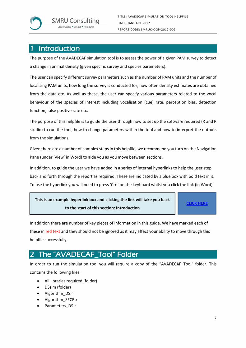
2 The “AVADECAF_Tool” Folder

In order to run the simulation tool you will require a copy of the “AVADECAF_Tool” folder. This

contains the following files:

All libraries required (folder)

DSsim (folder)

Algorithm_DS.r

Algorithm_SECR.r

Parameters_DS.r

This is an example hyperlink box and clicking the link will take you back

to the start of this section: Introduction CLICK HERE

8


DATE: JANUARY 2017


Parameters_SECR.r

script.r

Simulation_functions_DS.r

Simulation_functions_SECR.r

the loop for sa.r

simulations and parameters.xls

Navigate on your computer to the C drive. We recommend you create a folder called RRun. Copy the

“AVADECAF_Tool” folder provided and paste it in the RRun folder you just created.

Within the “AVADECAF_Tool” folder there are files that should be edited by the user and some files

that should NOT be edited by the user.

3 Installing R

Note: This simulation tool has been tested with R version 3.3.2 and specific libraries (see below). We

cannot guarantee it will be compatible with other versions. If, at the time of installing R onto your

computer a newer version has been released, we recommend you install version 3.3.2 to ensure

compatibility with the R script. This can be done through the link: https://cran.r-

project.org/bin/windows/base/old/

Windows users: The latest version of R can be downloaded from: https://cran.r-

project.org/bin/windows/base/

Mac users: https://cran.r-project.org/bin/macosx/

Click on the Download link at the top of the page to download the .exe file

Open the .exe file.

1. This will open a new window called Setup – R for Windows. Click Next > to start the

installation process.

2. GNU General Public License information will then appear. Click Next >

3. When prompted to select the destination location it should automatically select the

following: C:\Program Files\R\. If not, browse to this location. Click Next >

4. When prompted to select components make sure all boxes are ticked (Core Files, 32-bit

Files, 64-bit Files and Message translations). Click Next >

5. When prompted to customize startup options select No (accept defaults). Click Next >

Details of which files can be edited by the user are outlined in section 7

The simulation files CLICK HERE

https://cran.r-project.org/bin/windows/base/old/

https://cran.r-project.org/bin/windows/base/old/

https://cran.r-project.org/bin/windows/base/

https://cran.r-project.org/bin/windows/base/

9


DATE: JANUARY 2017


6. When prompted to select the start menu folder accept the automatic R shortcut. Click Next

>

7. When prompted to select additional tasks tick the following box: associate R with .RData

files. Click Next >

8. R will then install on your computer

9. Click Finish to exit setup

10


DATE: JANUARY 2017


4 Installing RStudio

Disclaimer: This simulation tool has been tested with RStudio version 0.99.903. We cannot guarantee

it will be compatible with other versions. If, at the time of installing RStudio onto your computer a

newer version has been released, we recommend you install version 0.99.903 to ensure compatibility

with the R script. This can be done through the link: https://support.rstudio.com/hc/en-

us/articles/206569407-Older-Versions-of-RStudio

RStudio is an integrated development environment for R. For the novice or less experienced R user,

RStudio is often considered to be a much more user friendly programme to use than R itself. RStudio

works by running alongside R and it simply provides a more user friendly interface to work from.

Therefore, you cannot run RStudio without having R installed on your computer.

The latest version of RStudio can be downloaded from:

https://www.rstudio.com/products/rstudio/download/

Click on the Installer link for Windows Vista/7/8/10 to download the .exe file

Open the .exe file.

1. This will open a new window called Setup – RStudio Setup. Click Next > to start the

installation process

2. When prompted to select the destination location it should automatically select the

following: C:\Program Files\RStudio. If not, browse to this location. Click Next >

3. When prompted to select the start menu folder accept the automatic RStudio shortcut. Click

Install

4. RStudio will then install on your computer

5. Click Finish to exit setup.

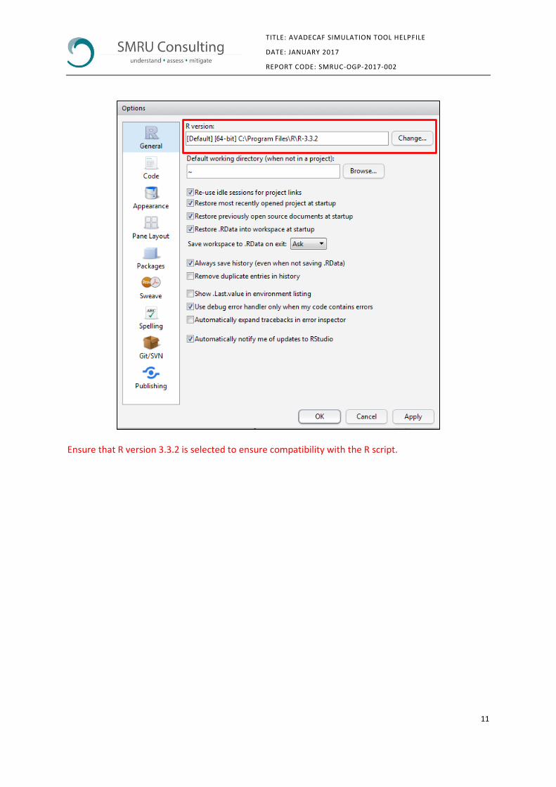
If for any reason you have multiple versions of R installed on your computer, you can specify which R

version you wish to run in RStudio. This is done by opening RStudio and selecting Tools > Global

Options:

https://support.rstudio.com/hc/en-us/articles/206569407-Older-Versions-of-RStudio

https://support.rstudio.com/hc/en-us/articles/206569407-Older-Versions-of-RStudio

https://www.rstudio.com/products/rstudio/download/

11


DATE: JANUARY 2017


Ensure that R version 3.3.2 is selected to ensure compatibility with the R script.

12


DATE: JANUARY 2017


5 Installing R Packages

Packages are the fundamental units of reproducible R code. They include reusable R functions, the

documentation that describes how to use them and sample data. The packages necessary to run this

simulation tool are listed in the file Libraries.r provided in the “AVADECAF_Tool” folder.

Disclaimer: This simulation tool has been tested with the following package versions. We cannot

guarantee this simulation tool will be compatible with other versions. We recommend you install the

version listed below to ensure compatibility with the R script.

Package: shapefiles Version: 0.7

Package: chron Version: 2.3-47

Package: splancs Version: 2.01-39

Package: mrds Version: 2.1.16

Package: optimx Version: 2013.8.7

Package: numDeriv Version: 2014.2-1

Package: mgcv Version: 1.8-12

Package: Rsolnp Version: 1.16

Package: rmarkdown Version: 1.0

Package: knitr Version: 1.14.11

Package: printr Version 0.0.6

Package: secr

It is possible that these versions listed above are older versions than the current versions available on

the CRAN library.

There are 2 ways to install all required packages and dependencies

1) Use the files provided in the “AVADECAF_Tool” folder (this is the easiest way)

2) Install packages and specific versions yourself through RStudio (proficient R users may prefer

to do it in this way)

5.1 Installing packages from the “AVADECAF_Tool” folder

All packages that the tool requires are included in the “AVADECAF_Tool” folder in the folder called

“All libraries required”.

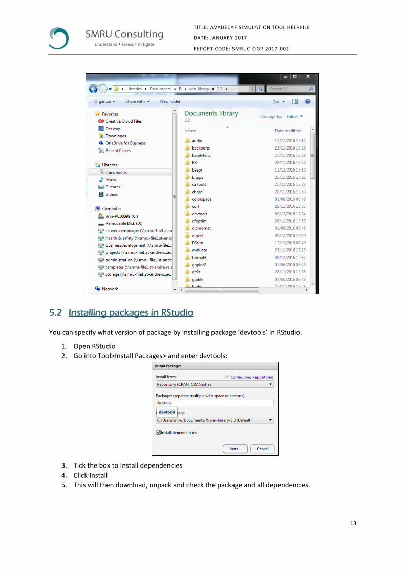
Navigate to the win-library on your computer. This is located at Documents\R\win-library\3.3 (Note:

this is the folder name even when you install version 3.3.2 as specified above). Copy all library folders

from the folder “All libraries required” in the “AVADECAF_Tool”folder, and paste them into the 3.3

folder in the win-library on your computer:

13


DATE: JANUARY 2017


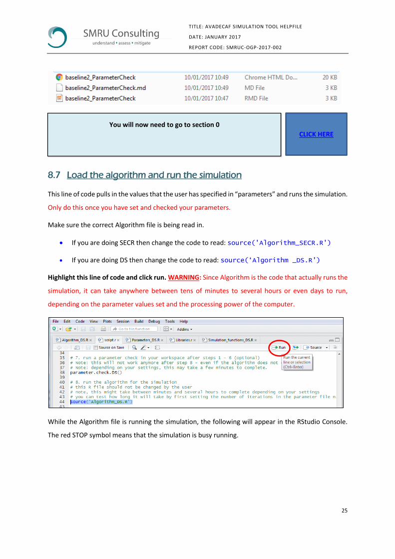
5.2 Installing packages in RStudio

You can specify what version of package by installing package ‘devtools’ in RStudio.

1. Open RStudio

2. Go into Tool>Install Packages> and enter devtools:

3. Tick the box to Install dependencies

4. Click Install

5. This will then download, unpack and check the package and all dependencies.

14


DATE: JANUARY 2017


Copy and paste the following blue text into the Console window in order to install the correct versions

of the packages:

require(devtools)

install_version('shapefiles', version='0.7', repros="http://cran.us.r-project.org")

install_version('chron', version='2.3-47', repros="http://cran.us.r-project.org")

install_version('splancs', version='2.01-39', repros="http://cran.us.r-project.org")

install_version('mrds', version='2.1.16', repros="http://cran.us.r-project.org")

install_version('optimx', version='2013.8.7', repros="http://cran.us.r-project.org")

install_version('numDeriv', version='2014.2-1', repros="http://cran.us.r-project.org")

install_version('mgcv', version='1.8-12', repros="http://cran.us.r-project.org")

install_version('Rsolnp', version='1.16', repros="http://cran.us.r-project.org")

install_version('rmarkdown', version='1.0', repros="http://cran.us.r-project.org")

install_version('knitr', version='1.14', repros="http://cran.us.r-project.org")

install.packages('printr', type = 'source', repos = c('http://yihui.name/xran', 'http://cran.rstudio.com'))

Next you need to put the package DSsim on your computer. Do NOT install this like the other packages

above. In the folder “FinalTool” provided, there is a folder called DSsim. Copy the entire DSsim folder.

Navigate on your computer to: Documents\R\win-library\3.3 (Note: this is the folder name even when

you install version 3.3.2 as specified above). Paste the DSsim folder into this documents library

Documents\R\win-library\3.3 alongside the other packages and dependencies that have been

installed.

15


DATE: JANUARY 2017


You can check the versions of all packages and dependencies installed on your computer by:

1. Opening RStudio

2. Typing the following code into the console: installed.packages()

This will then list all packages installed on your computer along with information on where the

package is stored (LibPath) and what version is installed:

16


DATE: JANUARY 2017


If the version listed does not match one of the versions listed as tested above, then we recommend

you install the version listed above to ensure compatibility with the R script.

17


DATE: JANUARY 2017


6 Organising folders

We highly recommend that you create a separate folder for each different simulation you run. This

avoids the problem of R overwriting any previously saved files. This is easy to accidentally do and so

we recommend keeping separate folders for each simulation and a record of how each simulation

differs to the others you have run.

For example:

Simulation1 – could have a cue rate of 1000 and a spacing of 7.5

Simulation2 – could have a cue rate of 2000 and a spacing of 7.5

Simulation3 – could have a cue rate of 2000 and a spacing of 15

Etc…

We recommend maintaining a pristine copy of the tool code. To create new folders, copy and paste

the “AVADECAF_Tool” folder and re-name it something sensible that relates to the simulation you are

running e.g. FinalTool_Simulation1

18


DATE: JANUARY 2017


7 The simulation files

Within the “AVADECAF_Tool” folder there are files that should be edited by the user and some files

that should NOT be edited by the user.

7.1 script.R

This is the main control centre for the tool. It pulls in the other files in the correct sequence in order

to run the tool.

7.2 Parameters_DS.R and Parameters_SECR.R

This is where the user specifies all the survey design parameters and the vocalisation parameters for

the species of interest.

The survey design parameters include: the number of PAM units and the number of localising PAM

units, how long the survey is conducted for, how often density estimates are obtained from the data

etc.

The parts of this file that should be edited by the user are outlined in

section 8 script.r CLICK HERE

19


DATE: JANUARY 2017


The vocalisation parameters include: vocalisation (cue) rate, perception bias, detection function, false

positive rate etc.

7.3 Simulation_functions_DS.R and Simulation_functions_SECR.R

This file specifies the functions that will be used in the file “Algorithm” in order for the tool to run. It

checks the survey and vocalisation parameters that the user has specified in “parameters” and returns

error messages if any of the parameters have been incorrectly set.

The user should NOT edit this file at all.

7.4 Algorithm.R

This is the file that runs the simulation. It pulls in the values that the user has specified in “parameters”.

The user should NOT edit this file at all.

The parts of this file that should be edited by the user are outlined in

section 9 Parameters_DS.r CLICK HERE

20


DATE: JANUARY 2017


8 script.r

Navigate to C:\RRun. Open the simulation folder that you wish to work on eg: FinalTool_Simulation1

Double click on the R file script.r. This will open the R file in the script window in RStudio.

8.1 Set the working directory

Click on the tab Session then Set Working Directory then Choose Directory and browse to the RRun

folder on the C drive. Select the simulation folder you are working on eg: “FinalTool_Simulation1” and

click Select Folder.

The following text will appear in the Console in RStudio:

> setwd("C:/RRun/FinalTool_Simulation1")

21


DATE: JANUARY 2017


This means that from now on, all files that R accesses will be from this FinalTool_Simulation1 folder.

8.2 Name your analysis

This allows you to give your simulation a name. This should be set as something clear that you can

come back to and understand. All files produced from this simulation will bear this name so it is

important to choose it sensibly.

For example, perhaps you wish to change the density of animals to 50 but keep all other parameters

the same as the baseline/default. For this we would recommend naming your analysis something like:

sim.name <- "Density50"

Highlight this line of code and click run.

If you are running many simulations with different parameters, we’d recommend maintaining a

spreadsheet with all of your key settings and parameter values (and your names corresponding to

each folder). We have provided an Excel template for this (simulations and parameters.xls).

8.3 Choose an analysis method

This code can do 2 types of simulations:

"DS" – which uses Distance sampling as the analysis method

We are now going to go through the steps in the file script.r. This will involve some moving between sections of this helpfile in order to set up the different files that are read into script.r or

to check an output file. When you need to move to a different section then an instruction box like this will direct you.

22


DATE: JANUARY 2017


"SECR" – which uses a Spatially Explicit Capture Recapture approach.

If you are doing DS then change the code to read: method = "DS"

If you are doing SECR then change the code to read: method = "SECR"


NOTE: The different analysis methods apply to different PAM circumstances (deployments/species),

therefore the user should refer to the main report before running this.

NOTE: These two analysis methods are very different and also incur very different run times (that is,

how long a simulation takes to run). For example, a typical run length for a DS (Distance) simulation is

20-60mins (this will depend on your parameters and RAM on your computer), whereas a typical SECR

(spatially explicit capture re-capture) simulation takes approximately 40-50 hours on a normal laptop

when running 3 cores.

8.4 Load the functions

Make sure the correct function file is being read in.

If you are doing DS then change the code to read: source('Simulation_functions_DS.R')

If you are doing SECR then change the code to read:

source('Simulation_functions_SECR.R')


23


DATE: JANUARY 2017


8.5 Set the parameters

Make sure the correct parameters file is being read in:

If you are doing DS then change the code to read: source(‘Parameters_DS.R')

If you are doing SECR then change the code to read: source(‘Parameters_SECR.R')

Once you have set up the parameters file with survey design and vocalisation parameters, you should

highlight this line of code in script.R and click run. Only do this once you have set your parameters.

8.6 Check the parameters

Only do this once you have set your parameters.

This will run a short set of code that checks the survey design and vocalisation parameters that you

have set in Parameters_DS (or Parameters_SECR). As is described further in section 9

Parameters_DS.r, there are certain parameters that have set upper and lower bounds for the values.

You will now need to go to section 9 Parameters_DS.r for instructions on

how to set the survey design and vocalisation parameters. CLICK HERE

24


DATE: JANUARY 2017


For example: cue rate cannot be a negative value, perception bias must be between 0 and 1 and error

must be between 0-100 etc. This parameter.check will highlight if there are any values set in the

parameters that are out of bounds for the simulation.

Highlight this line of code and click run. This usually takes a few minutes to run.

While the parameter.check is running you will see this in the RStudio console:

One the parameter.check has run the red STOP symbol will disappear and it will produce a line of code

in the RStudio Console that says it has created new output files. For example:

This means that there are new files in your simulation folder:

25


DATE: JANUARY 2017


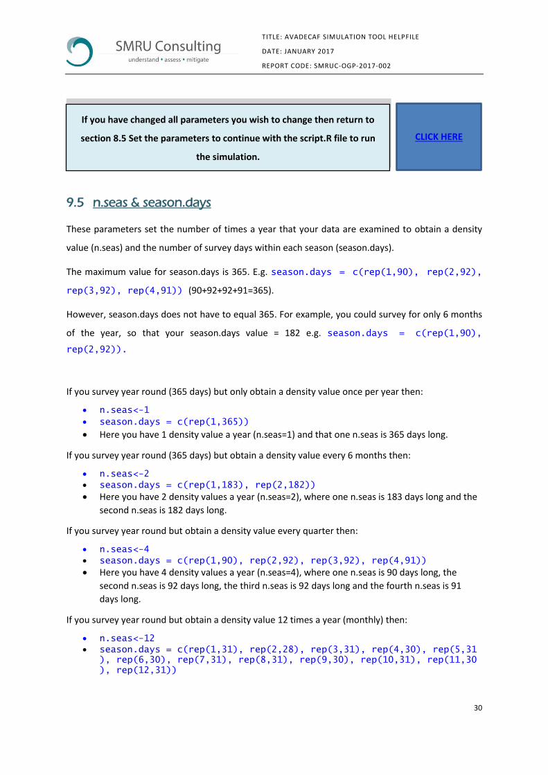
8.7 Load the algorithm and run the simulation

This line of code pulls in the values that the user has specified in “parameters” and runs the simulation.

Only do this once you have set and checked your parameters.

Make sure the correct Algorithm file is being read in.

If you are doing SECR then change the code to read: source('Algorithm_SECR.R')

If you are doing DS then change the code to read: source(‘Algorithm _DS.R')

Highlight this line of code and click run. WARNING: Since Algorithm is the code that actually runs the

simulation, it can take anywhere between tens of minutes to several hours or even days to run,

depending on the parameter values set and the processing power of the computer.

While the Algorithm file is running the simulation, the following will appear in the RStudio Console.

The red STOP symbol means that the simulation is busy running.

You will now need to go to section 0

Parameter Check to check that the parameters you have specified are

within the bounds of the allowed values.

CLICK HERE

26


DATE: JANUARY 2017


If you need to stop the simulation, then click the red STOP button. But after you do that it is essential

that you run the following line of code:

stopCluster(cl)

Note: you do not need to run this code if the code ran successfully, only if you manually stopped it.

8.8 Get the results

Only do this once algorithm has finished running the simulation.

This will export the results of the simulation.

Highlight these 3 lines of code and click run.

This will create an .html file with the outputs in your simulation folder:

27


DATE: JANUARY 2017


You have now finished with script.r. Please go to section 11 Outputs to

check the outputs of the simulation. CLICK HERE

28


DATE: JANUARY 2017


9 Parameters_DS.r

There are 301 lines of code in Parameters_DS.r. Most of these are instructions and lines of code that

the user should NOT alter. Instructions and explanations are shown in green and preceded by a # in

the code files.

This section of the helpfile is going to walk through how to set up a basic simulation model. This basic

simulation model does not allow for changes in the parameters (such as density, cue rate etc) by year

or season nor does it add hotspot areas to the survey region.

Modifications to the simulation tool to include these additional layers of information can be found later

in this document in the section: More complex models.

To run the basic simulation model the following lines of code need to be changed by the user:

9.1 n.cl

Computers have multiple cores of memory available for processing. In order to decrease the time

taken to run the simulation, the user can use parallel computing. This makes use of multiple cores on

the computer and sets the cores running the code simultaneously. The higher the number of cores

used the faster the simulation will run; however less memory will available on the computer for other

processes at the same time.

First you need to enter the following code to find out how many cores your computer has:

> detectCores() [1] 4

This output states that the computer has 4 cores.

It is recommended that the user should leave 1 or 2 cores available for other processes on the

computer. Therefore in this instance, it is recommended that the number of cores to be used to 2.

This is done by changing the lines of code so that it reads:

n.cl = 2

If you have changed all parameters you wish to change then return to

section 8.5 Set the parameters to continue with the script.R file to run

the simulation.

CLICK HERE

29


DATE: JANUARY 2017


9.2 computer

This allows you to change the name of the computer you are working on. It is a good idea to keep

track of what simulations were run on what computer for later reference. The default code reads

computer=”squid” as Squid is the name of the supercomputer at CREEM where this code was created

and tested. You should change this to something relevant to your computer. For example:

computer = "JIP_laptop"

9.3 n.sim

This sets the number of simulation runs for power analysis. 1000 is the default/recommended

minimum number of iterations for each simulation.

It is recommended that you first test the code with 10 iterations, for example, before setting it up to

run 1000 iterations. This way it will run 10 iterations pretty quickly so that you can see if there are any

errors in the code. The last thing you want is to set up the computer to run 1000 iterations overnight

and come back in the morning to an error message and no results!

9.4 n.yrs

This sets the number of years that the survey is conducted for. This is set to 10 as the default. We

recommend that you keep it at 10.

It is worth noting that your power to detect a change will increase with increasing survey years;

however it will also take longer for the model to run. For example:

n.yrs <- 10 will take approximately half as long to run as n.yrs <- 20



the simulation.



the simulation.

CLICK HERE

CLICK HERE

30


DATE: JANUARY 2017


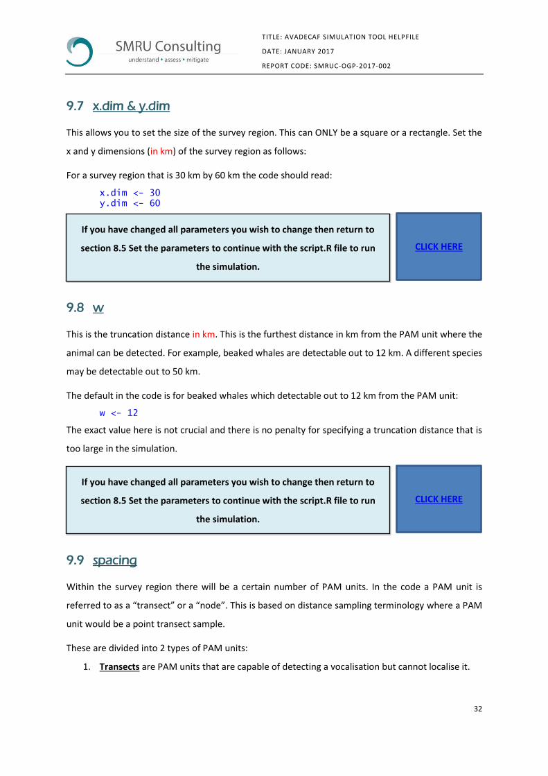
9.5 n.seas & season.days

These parameters set the number of times a year that your data are examined to obtain a density

value (n.seas) and the number of survey days within each season (season.days).

The maximum value for season.days is 365. E.g. season.days = c(rep(1,90), rep(2,92),

rep(3,92), rep(4,91)) (90+92+92+91=365).

However, season.days does not have to equal 365. For example, you could survey for only 6 months

of the year, so that your season.days value = 182 e.g. season.days = c(rep(1,90),

rep(2,92)).

If you survey year round (365 days) but only obtain a density value once per year then:

n.seas<-1

season.days = c(rep(1,365))

Here you have 1 density value a year (n.seas=1) and that one n.seas is 365 days long.

If you survey year round (365 days) but obtain a density value every 6 months then:

n.seas<-2 season.days = c(rep(1,183), rep(2,182))

Here you have 2 density values a year (n.seas=2), where one n.seas is 183 days long and the

second n.seas is 182 days long.

If you survey year round but obtain a density value every quarter then:

n.seas<-4 season.days = c(rep(1,90), rep(2,92), rep(3,92), rep(4,91))

Here you have 4 density values a year (n.seas=4), where one n.seas is 90 days long, the

second n.seas is 92 days long, the third n.seas is 92 days long and the fourth n.seas is 91

days long.

If you survey year round but obtain a density value 12 times a year (monthly) then:

n.seas<-12 season.days = c(rep(1,31), rep(2,28), rep(3,31), rep(4,30), rep(5,31

), rep(6,30), rep(7,31), rep(8,31), rep(9,30), rep(10,31), rep(11,30), rep(12,31))



the simulation.

CLICK HERE

31


DATE: JANUARY 2017


You can specify the code so that a season (such as Winter) can start in December and end in February

and so is split over two years. For this the code would look like:

season.days = c(rep(1,59),rep(2,92), rep(3,92),rep(4,91),rep(1,31))

Season 1 starts on Jan 1st and runs for a total of 59 days ending on Feb 28th.

Season 2 starts on March 1st and runs for a total of 92 days ending on May 31st.

Season 3 starts on June 1st and runs for a total of 92 days ending on Aug 31st.

Season 4 starts on Sept 1st and runs for a total of 91 days ending on Nov 30th.

Season 1 starts on Dec 1st and runs for a total of 31 days ending on Dec 31st.

This gives a total of 365 days (the code does not account for a leap year)

Season 1 is listed twice because the entire season (eg: winter in the UK) runs between December and

February and so is split between years.

9.6 time

This sets the amount of time that in surveyed in a single day in seconds.

The default is constant 24hour monitoring (86,400 seconds per day):

time <- 24 * 60 * 60

This can be adjusted depending on the duty cycle of the PAM unit.

It doesn’t matter how you specify the duty cycle.

For example: to record only 12 hours a day (43,200 sec) you can enter:

time <- 12 * 60 * 60 time <- 24 * 30 * 60 time <- 24 * 60 * 30



the simulation.



the simulation.

CLICK HERE

CLICK HERE

32


DATE: JANUARY 2017


9.7 x.dim & y.dim

This allows you to set the size of the survey region. This can ONLY be a square or a rectangle. Set the

x and y dimensions (in km) of the survey region as follows:

For a survey region that is 30 km by 60 km the code should read:

x.dim <- 30 y.dim <- 60

9.8 w

This is the truncation distance in km. This is the furthest distance in km from the PAM unit where the

animal can be detected. For example, beaked whales are detectable out to 12 km. A different species

may be detectable out to 50 km.

The default in the code is for beaked whales which detectable out to 12 km from the PAM unit:

w <- 12

The exact value here is not crucial and there is no penalty for specifying a truncation distance that is

too large in the simulation.

9.9 spacing

Within the survey region there will be a certain number of PAM units. In the code a PAM unit is

referred to as a “transect” or a “node”. This is based on distance sampling terminology where a PAM

unit would be a point transect sample.

These are divided into 2 types of PAM units:

1. Transects are PAM units that are capable of detecting a vocalisation but cannot localise it.



the simulation.



the simulation.

CLICK HERE

CLICK HERE

33


DATE: JANUARY 2017


2. Fancy nodes are PAM units that are capable of both detecting a vocalisation and measuring

the range to that vocalisation.

In order to randomly place the PAM units within the survey region we use the DSsim package. What

this means in practice is that we cannot tell the code the number of PAM units we want to place in

the survey region. Instead we tell the code what the spacing is between PAM units. For example, a

spacing of 7.5 will place 32 PAM units in a survey region that is 30x60 km.

You can check the number of PAM units and fancy nodes placed in the study region when you run

parameter.check.DS() in the script file.

9.10 nested.space

The nested space describes how the fancy nodes are spread out throughout the survey region.

What it means is “how far (in terms of PAM units) do I have to move in x and y space before I reach a

fancy node?”.

If all PAM units are fancy nodes then the nested space is 1 because you have to move 1 unit in x or y

space from one fancy node to get to the next fancy node

nested.space <- c(1)

If every other PAM unit is a fancy node then the nested space is 2 because you have to move 2 units

in x or y space from one fancy node to get to the next fancy node:


Nested Space = 3 means you have to move 3 units in x or y space from one fancy node to get to the

next fancy node:




the simulation.

CLICK HERE

34


DATE: JANUARY 2017


You can check the number of PAM units and fancy nodes placed in the study region when you run

parameter.check.DS() in the script file.

9.11 sigma1

This contributes to setting the detection function parameters.

Sigma is the scale parameter of the half-normal detection function which, together with the truncation

distance (w), defines the average detection probabilities.

For smaller values of sigma your probability of detection decreases rapidly with distance.

Figure 1 Four examples of a half-normal detection function, each with a different scale (sigma) parameter.



the simulation.

CLICK HERE

35


DATE: JANUARY 2017


9.12 sigma.cv

This sets the variance around the detection function. Sigma.cv lets the detection function vary across

the study region.

Figure 2 Examples of how an increase in sigma.cv affects the variability in detection functions in simulations for a default value of sigma = 2. For each plot, sigma is the same but the sigma.cv varies between 10% - 90% (i.e. 0.1 - 0.9).

9.13 error

The systematic error is a systematic distance bias in the detected distances.

Systematic distance bias is error that occurs when the estimated distances to cues are always

overestimated (or always underestimated) as can happen with factors related to, but not limited to,

temperature and salinity affecting sound speed profiles, sound refracting properties associated with

a particular location, background and/or sensor-specific errors.

The default in the code is no systematic error in the distances:

error <- NULL

Systematic bias is implemented in the simulation by adding or subtracting a distance to each cue that

is a percentage of the ‘true’ localisation distances. The magnitude of the systematic bias can be

specified by the user as a percentage multiplier on the cue distance estimate.



the simulation.



the simulation.

CLICK HERE

CLICK HERE

36


DATE: JANUARY 2017


Systematic error is expressed as a percentage of the detection distance and so can range from 0-100.

For example:

if your estimated detection distance was 100m and your error was 10 then your actual

detection distance is between 90 and 110m (100±10%).

If your estimated detection distance was 400m and your error was 10 then your actual

detection distance is between 360 and 440m (400±10%).

NOTE: Systematic and random error will introduce variability and bias to the system which will

decrease power and decrease accuracy in estimating animal densities and hence, in estimating trends

in densities.

It is HIGHLY unrealistic to run a simulation with error <- NULL as there will always be error in the

detected distances. We recommend changing the error value to at least 10: error <- 10

9.14 error.spread

Random error occurs when the distances are measured with low precision and can be over-or

underestimated.

The default in the code is no random error in the distances:

error.spread <- NULL

Random error is expressed as a proportion of the detection distance and so can range from 0-1.

NOTE: Systematic and random error will introduce variability and bias to the system which will

decrease power and decrease accuracy in estimating animal densities and hence, in estimating trends

in densities.

It is HIGHLY unrealistic to run a simulation with error.spread <- NULL as there will always be

error in your detection distances. We recommend changing the error.spread value to at least

0.1: error.spread <- 0.1



the simulation.

CLICK HERE

37


DATE: JANUARY 2017


9.15 d1

This sets the average density of animals in the survey region expressed as the number of animals per

km2.

If the density of animals in your survey region is 50 animals per km2 then the code gets changed to:

d1 <- 50/(1000)

9.16 decline

This sets the annual exponential decline in density. The default is set to 0.05 which means there is a

decline in the density of 5% per year.

You can make this higher or lower.

a 10% decline would be decline <- 0.10 a 2% decline would be decline <- 0.02

You can set this to zero if you want no annual exponential decline in density.

9.17 c1

This is the average cue production rate for the species of interest in your study region, given as the

number of cues produced per second. You can change this value to whatever cue production rate per

second you want.



the simulation.



the simulation.



the simulation.

CLICK HERE

CLICK HERE

CLICK HERE

38


DATE: JANUARY 2017


For example, if my species produced 1.5 cues per seconds the code would read:

c1 <- 1.5

c1 must be >0.

9.18 c.cv

This is the Coefficient of Variation (CV) for the cue production rate.

c.cv must be between 0 and 1.

Since the cue rate will be an estimated value (ie: obtained from the literature) then it will have an

associated precision value. This is often the coefficient of variation (CV). Sometimes the literature may

present other precision values such as standard deviation or standard error. Here is how you can

convert them to CV:

Standard Deviation: divide the standard deviation by the mean to get the CV.

Standard error: multiply the standard error by the square root of the sample size to get the

standard deviation. Then divide the standard deviation by the mean to get the CV.

Be careful when you set c.cv that you do not put a CV around c1 that makes c1 <0.

For example, if you have a cue rate of 0.1 then do not put c.cv<-0.3 as it the model will try (in at least

some of the 1,000 simulations) to put a c1 value of 0.1-0.3=-0.2 – which is not a valid value for c1.

If you enter a value that cannot run this will appear as an error message in the Parameter Check. You

will see a message that says:

"Your cue rates c all need to be larger than 0"



the simulation.



the simulation.

CLICK HERE

CLICK HERE

39


DATE: JANUARY 2017


9.19 a1

This is the perception bias. One of the assumptions in distance sampling is that all animals at the

transect are detected with certainty. In PAM surveys this assumption is violated if an animal is present

at the transect (PAM unit) but not vocalising, or it is present at the transect (PAM unit) but oriented

away from the PAM unit in such a way that vocalisations are missed by the PAM unit.

Therefore the value being entered here is the proportion of animals detected at the transect. For

example, if 65% of the animals present at the transect are detected then the code should read:

a1 <- c(0.65)

a1 must be between 0 and 1.

9.20 a.cv

This is the Coefficient of Variation (CV) for the perception bias.

a.cv must be between 0 and 1.

Since the perception bias will be an estimated value (ie: obtained from the literature) then it will have

an associated precision value. This is often the coefficient of variation (CV). Sometimes the literature

may present other precision values such as standard deviation or standard error. Here is how you can

convert them to CV:




Be careful when you set a.cv that you do not put a CV around a1 that makes it a value that is not

between 0 and 1.

For example, if you have a perception bias of 0.8 then do not put a.cv<-0.3 as it the model will try (in

at least some of the 1000 simulations) to put an a1 value of 0.8+0.3=1.1 – which is not a valid value

for a1.



the simulation.

CLICK HERE

40


DATE: JANUARY 2017




"Your perception bias a all need to be between 0 and 1"

9.21 f1

This is the false positive rate which is the proportion of detected cues that were not from the species

of interest. For example, in PAM surveys for beaked whales, dolphin clicks are often recorded as false

positives.

This is the false positive rate. The default value in the code is:

f1 <- 0.549

This means that 54.9% of the detections are false positives and the other 45.1% of the

vocalisations are correctly classified.

If you are surveying beaked whales while dolphins are also present, and you know that 50% of your

detections are false positives (dolphins not beaked whales) then the code should read:

f1 <- 0.5

f1 must be between 0 and 1.

9.22 f.cv

This is the Coefficient of Variation (CV) for the false positive rate.

f.cv must be between 0 and 1.

Since the false positive rate will be an estimated value (ie: obtained from the literature) then it will

have an associated precision value. This is often the coefficient of variation (CV). Sometimes the

literature may present other precision values. Here is how you can convert them to CV:



the simulation.



the simulation.

CLICK HERE

CLICK HERE

41


DATE: JANUARY 2017





Be careful when you set f.cv that you do not put a CV around f1 that makes it a value that is not

between 0 and 1.

For example, if you have a false positive rate of 0.8 then do not put f.cv<-0.3 as it the model will try

(in at least some of the 1000 simulations) to put an a1 value of 0.8+0.3=1.1 – which is not a valid value

for f1.



"Your false positive rates f all need to be between 0 and 1"

If you have reached the end of all the parameters the user should change

for a basic model. Please return to section 8.5 Set the parameters to

continue with the script.R file to run the simulation.

CLICK HERE

42


DATE: JANUARY 2017


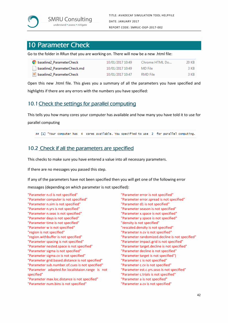
10 Parameter Check

Go to the folder in RRun that you are working on. There will now be a new .html file:

Open this new .html file. This gives you a summary of all the parameters you have specified and

highlights if there are any errors with the numbers you have specified:

10.1 Check the settings for parallel computing

This tells you how many cores your computer has available and how many you have told it to use for

parallel computing

10.2 Check if all the parameters are specified

This checks to make sure you have entered a value into all necessary parameters.

If there are no messages you passed this step.

If any of the parameters have not been specified then you will get one of the following error

messages (depending on which parameter is not specified):

"Parameter n.cl is not specified" "Parameter computer is not specified" "Parameter n.sim is not specified" "Parameter n.yrs is not specified" "Parameter n.seas is not specified" "Parameter days is not specified" "Parameter time is not specified" "Parameter w is not specified" "region is not specified" "region.withbuffer is not specified" "Parameter spacing is not specified" "Parameter nested.space is not specified" "Parameter sigma is not specified" "Parameter sigma.cv is not specified" "Parameter grid.based.distance is not specified" "Parameter sub.number.of.cues is not specified" "Parameter adapted.for.localistaion.range is not specified" "Parameter max.loc.distance is not specified" "Parameter num.bins is not specified"

"Parameter error is not specified" "Parameter error.spread is not specified" "Parameter d1 is not specified" "Parameter season is not specified" "Parameter x.space is not specified" "Parameter y.space is not specified" "density is not specified" "rescaled.density is not specified" "Parameter n.cv is not specified" "Parameter randomized.decline is not specified" "Parameter impact.grid is not specified" "Parameter target.decline is not specified" "Parameter decline is not specified" "Parameter target is not specified") "Parameter c is not specified" "Parameter c.cv is not specified" "Parameter est.c.yrs.seas is not specified" "Parameter c.trials is not specified" "Parameter a is not specified" "Parameter a.cv is not specified"

43


DATE: JANUARY 2017


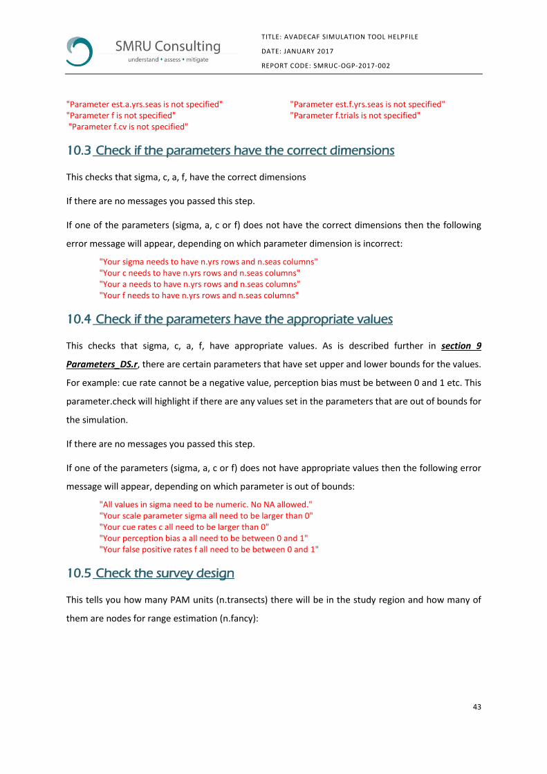
"Parameter est.a.yrs.seas is not specified" "Parameter f is not specified" "Parameter f.cv is not specified"

"Parameter est.f.yrs.seas is not specified" "Parameter f.trials is not specified"

10.3 Check if the parameters have the correct dimensions

This checks that sigma, c, a, f, have the correct dimensions


If one of the parameters (sigma, a, c or f) does not have the correct dimensions then the following

error message will appear, depending on which parameter dimension is incorrect:

"Your sigma needs to have n.yrs rows and n.seas columns" "Your c needs to have n.yrs rows and n.seas columns" "Your a needs to have n.yrs rows and n.seas columns" "Your f needs to have n.yrs rows and n.seas columns"

10.4 Check if the parameters have the appropriate values

This checks that sigma, c, a, f, have appropriate values. As is described further in section 9

Parameters_DS.r, there are certain parameters that have set upper and lower bounds for the values.

For example: cue rate cannot be a negative value, perception bias must be between 0 and 1 etc. This

parameter.check will highlight if there are any values set in the parameters that are out of bounds for

the simulation.


If one of the parameters (sigma, a, c or f) does not have appropriate values then the following error

message will appear, depending on which parameter is out of bounds:

"All values in sigma need to be numeric. No NA allowed." "Your scale parameter sigma all need to be larger than 0" "Your cue rates c all need to be larger than 0" "Your perception bias a all need to be between 0 and 1" "Your false positive rates f all need to be between 0 and 1"

10.5 Check the survey design

This tells you how many PAM units (n.transects) there will be in the study region and how many of

them are nodes for range estimation (n.fancy):

44


DATE: JANUARY 2017


10.6 Check the detection function

This shows you what your detection function looks like:

10.7 Check the region, density and transects

This shows you what your study region looks like.

If you have specified hotspots in your survey region (as is the default) then you will be able to see

them in your survey region plot here (white and yellow) and the position of the PAM units: blue dot =

simple node (detection only), green dot = fancy node (range estimation node).

45


DATE: JANUARY 2017


11 Outputs

Once the script.r code has run, it will produce a .html file as an output.

This provides you with the outputs of the simulation.

11.1 Power to detect a change

In the tool a GLM is fitted to the data for each individual iteration run. For example, if n.sim=1,000

then 1,000 iterations are run and 1,000 GLMs are created to determine if a decline can be detected in

each iteration. The output file gives the percentage of iterations with a p-value<0.05, denoting a

significant decline parameter in the fitted GLM.

This means that:

76.4% of the iterations had a GLM p-value of 0.1

61.9% of the iterations had a GLM p-value of 0.05 (a significant parameter decline was

detected)

32.5% of the iterations had a GLM p-value of 0.01 (a highly significant parameter decline was

detected)

You have now finished checking your parameter values. Please go to

section 8.7 Load the algorithm and run the simulation to continue with

the script.R file and run the simulation.

CLICK HERE

46


DATE: JANUARY 2017


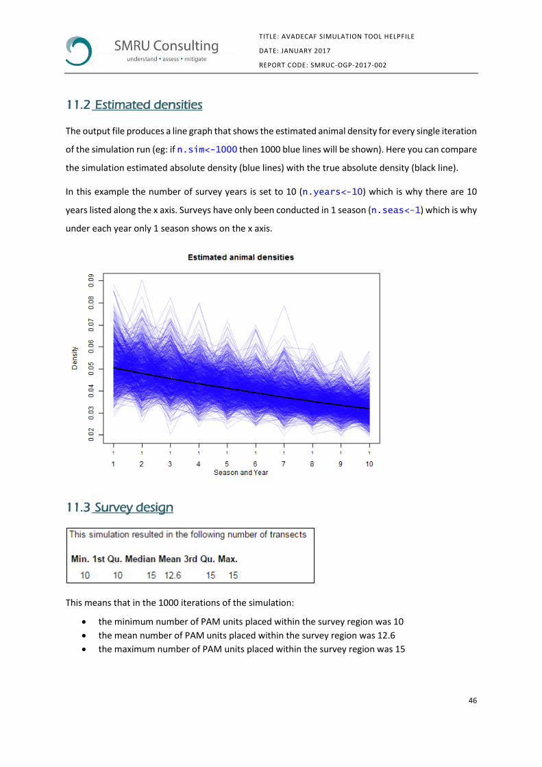
11.2 Estimated densities

The output file produces a line graph that shows the estimated animal density for every single iteration

of the simulation run (eg: if n.sim<-1000 then 1000 blue lines will be shown). Here you can compare

the simulation estimated absolute density (blue lines) with the true absolute density (black line).

In this example the number of survey years is set to 10 (n.years<-10) which is why there are 10

years listed along the x axis. Surveys have only been conducted in 1 season (n.seas<-1) which is why

under each year only 1 season shows on the x axis.

11.3 Survey design

This means that in the 1000 iterations of the simulation:

the minimum number of PAM units placed within the survey region was 10

the mean number of PAM units placed within the survey region was 12.6

the maximum number of PAM units placed within the survey region was 15

47


DATE: JANUARY 2017


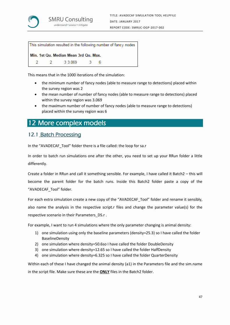
This means that in the 1000 iterations of the simulation:

the minimum number of fancy nodes (able to measure range to detections) placed within

the survey region was 2

the mean number of number of fancy nodes (able to measure range to detections) placed

within the survey region was 3.069

the maximum number of number of fancy nodes (able to measure range to detections)

placed within the survey region was 6

12 More complex models

12.1 Batch Processing

In the “AVADECAF_Tool” folder there is a file called: the loop for sa.r

In order to batch run simulations one after the other, you need to set up your RRun folder a little

differently.

Create a folder in RRun and call it something sensible. For example, I have called it Batch2 – this will

become the parent folder for the batch runs. Inside this Batch2 folder paste a copy of the

“AVADECAF_Tool” folder.

For each extra simulation create a new copy of the “AVADECAF_Tool” folder and rename it sensibly,

also name the analysis in the respective script.r files and change the parameter value(s) for the

respective scenario in their Parameters_DS.r .

For example, I want to run 4 simulations where the only parameter changing is animal density:

1) one simulation using only the baseline parameters (density=25.3) so I have called the folder

BaselineDensity

2) one simulation where density=50.6so I have called the folder DoubleDensity

3) one simulation where density=12.65 so I have called the folder HalfDensity

4) one simulation where density=6.325 so I have called the folder QuarterDensity

Within each of these I have changed the animal density (a1) in the Parameters file and the sim.name

in the script file. Make sure these are the ONLY files in the Batch2 folder.

48


DATE: JANUARY 2017


Now you can open the loop for sa.r file.

You need to set the working directory to the parent folder that you just created Batch2 – see

highlighted lines in the code below:

# SA1b script

curwd<-"C:/RRun/Batch2"

setwd("C:/RRun/Batch2")

dirx <- dir()

for (i in 1:length(dirx)){

newwd<-paste(curwd,"/",dirx[i],sep="")

setwd(newwd)

rm(list=ls())

source("script.R")

curwd <- "C:/RRun/Batch2"

setwd(curwd)

dirx <- dir()

}

12.2 Changing other parameters

Out with the basic model described above in section 9 Parameters_DS.r, there are many other

parameters that can be changed to make the mode more complex and more realistic. This are

described in turn below.

49


DATE: JANUARY 2017


12.2.1 Change the detection function scale parameter by season

The default code is a half normal detection function with a scale parameter of 2 and no seasonal

change:

sigma1 <- 2

sigma <- sigma1 * c(1,1,1,1)[1:n.seas]

Remember: For smaller values of sigma your probability of detection decreases rapidly with distance.

Figure 3 four examples of a half-normal detection function, each with a different scale (sigma) parameter.

You can adjust this so that the detection function scale parameter changes during certain seasons. For

example we can make the detection function scale parameter higher in the spring and summer

periods:

sigma1 <- 2

sigma <- sigma1 * c(1,1.5,1.5,1)[1:n.seas]

Here the detection function scale parameter is 50% higher in seasons 2 and 3. This means that in

seasons 2 and 3 your probability of detection with increasing distance is better than in months 1 and

4.

12.2.2 Change the detection function scale parameter by year

You can change the detection function scale parameter by year. The default in the code is for no

annual change in the detection function scale parameter:

sigma.bias <- 0

This can be changed so that it increases by a set percentage each year.

50


DATE: JANUARY 2017


sigma.bias <- 0.05 means that the detection function scale parameter increases by

5% annually

sigma.bias <- 0.1 means that the detection function scale parameter increases by 10%

annually

12.2.3 Change density by season

This may be applicable to certain species that are known to migrate through an area and so will be

present in higher densities at certain times of the year.

The default code is a density of 0.0253 animals/km2 and no seasonal change:

d1 <- 25.3/(1000)

season <- c(1,1,1,1)[1:n.seas]

You can adjust this so that the density gets higher during certain seasons. For example we can make

the density higher in the spring and summer periods:

d1 <- 25.3/(1000)

season <- c(1,1.5,1.5,1)[1:n.seas]

Here the density is 50% higher in seasons 2 and 3. This means that the density in seasons 1

and 4 =0.0253 animals/km2 while the density in seasons 2 and 3 =0.03795 animals/km2

(25.3*1.5/1000)

12.2.4 Change cue production rate by season

This may be particularly applicable to certain species (e.g: humpback whales) that are known to

vocalise more during certain periods of the year (such as the mating season) compared to other times

of the year.

The default code is a cue rate of 0.407 cues/sec and no seasonal change:

c1 <- 0.407

c <- c1 * c(1,1,1,1)[1:n.seas]

You can adjust this so that the cue rate gets higher during certain seasons. For example we can make

the cue rate higher in the spring and summer periods:

c1 <- 0.407

c <- c1 * c(1,1.5,1.5,1)[1:n.seas]

Here the cue rate is 50% higher in seasons 2 and 3. This means that the cue rate in seasons 1

and 4=0.407 while the cue rate in seasons 2 and 3=0.6105 (0.407*1.5)

51


DATE: JANUARY 2017


12.2.5 Change cue production rate by year

You can change the cue production rate by year. The default in the code is for no annual change in

cue rate:

c.bias <- 0


c.bias <- 0.05 means that the cue rate increases by 5% annually

c.bias <- 0.1 means that the cue rate increases by 10% annually

12.2.6 Creating overdispersion in the cue rate

Counts of cues at each node are generated from a negative binomial distribution to allow for extra-

Poisson variability, typical of biological datasets.

With the negative binomial distribution (unlike with the Poisson), the variance can be larger than the

mean, and thus the variance inflation factor n.cv needs to be defined.

This parameter reflects the proportion of overdispersion in the cue data (e.g. 1.2 is a 20% over-

dispersion in cue count).

Note that when n.cv = 1, the negative binomial distribution reduces to a Poisson distribution when

using distance sampling methods, i.e. for method = “DS”.

12.2.7 Change perception bias by season

The default code is a perception bias of 0.07 and no seasonal change:

a1 <- c(0.07)

a <- a1 * c(1,1,1,1)[1:n.seas]

You can change this so that the perception increases by 50% in the summer for example. The code

would be changed to:

a1 <- c(0.07)

a <- a1 * c(1,1.5,1,1)[1:n.seas]

Here the perception bias is 50% higher in season 2 (summer). This means that the

perception bias in seasons 1, 3 and 4=0.07 while the perception bias in season 2=0.105

(0.07*1.5)

12.2.8 Change perception bias by year

You can change the perception bias by year. The default in the code is for no annual change in

perception bias:

52


DATE: JANUARY 2017


a.bias <- 0


• a.bias <- 0.05 means that the perception bias increases by 5% annually

• a.bias <- 0.1 means that the perception bias increases by 10% annually

Be careful when you change a.bias that you do not make a1 a non-valid value. a1 must be between 0

and 1.



## [1] "Your perception bias values a all need to be between 0 and 1"

12.2.9 Change false positive rate by season

This may be particularly applicable if another species with similar vocalisations as your target species

enters the study region at certain times of the year. For example, dolphin vocalisations can occur as a

false positive in beaked whale studies. If the dolphins are only present in the study region at certain

times of the year e.g: summer, then your false positive rate will be different in the summer.

The default code is a false positive rate of 0.547 and no seasonal change:

f1 <- 0.547

f <- f1 * c(1,1,1,1)[1:n.seas]

You can change this to match the beaked whale and dolphin scenario described above. Let’s assume

that the false positive rate increases by 50% in the summer because of the presence of dolphins. The

code would be changed to:

f1 <- 0.547

f <- f1 * c(1,1.5,1,1)[1:n.seas]

Here the false positive rate is 50% higher in season 2 (summer). This means that the false

positive rate in seasons 1, 3 and 4=0.547 while the false positive rate in season 2=0.8205

(0.547*1.5)

12.2.10 Change false positive rate by year

You can change the false positive rate by year. The default in the code is for no annual change in false

positive rate:

f.bias <- 0

53


DATE: JANUARY 2017



f.bias <- 0.05 means that the false positive rate increases by 5% annually

f.bias <- 0.1 means that the false positive rate increases by 10% annually

This may be applicable if another species with similar vocalisations as your target species are also

present in the study region. For example, dolphin vocalisations can occur as a false positive in beaked

whale studies. If the local population of dolphins is increasing annually then the false positive rate in

the beaked whale study may increase annually.

Be careful when you change f.bias that you do not make f1 a non-valid value. f1 must be between 0

and 1.

For example: if your f1 value is 0.8 then you cannot have an f.bias value of 0.1 (a 10% annual increase)

because after 4 years your f1 value would be >1 and not allowed.

year f1

1 0.80

2 0.88

3 0.97

4 1.06



## [1] "Your false positive rates f all need to be between 0 and 1"

12.2.11 Maximum localisation distance

The code allows you to define the largest distance at which a detection can be localised. The default

in the code is:

max.loc.distance=ifelse(adapted.for.localisation.range==F,w,.5)

This means that if adapted.for.localisation.range==F then the largest distance at which a

detection can be localised is w (the truncation distance in km). Ie: if your truncation width (w) is 12

km then you are able to localise a cue out to a distance of 12 km.

If adapted.for.localisation.range==T then the largest distance at which a detection can be

localised can be manually set. For example:

54


DATE: JANUARY 2017


max.loc.distance=ifelse(adapted.for.localisation.range==F,w,.5)

this code means that if adapted.for.localisation.range==F then the localisation distance is

set to w, and if adapted.for.localisation.range==T then the localisation distance is set to 0.5

km.

You can change max.loc.distance to any value less than w (the truncation width). Ie: to make

your localisation distance 2 km then the code gets changed to:

adapted.for.localisation.range==T

max.loc.distance=ifelse(adapted.for.localisation.range==F,w,2)

which means that detections are localised out to 2 km and beyond that detections are lumped into

one distance bin (from max.loc.distance to truncation distance "w").

12.2.12 Randomised decline

In the code you can set the annual exponential decline in densities. The default in the code is an

exponential 5% annual decline every year over the study period:

decline <- 0.05

randomized.decline = FALSE

If you change randomized decline to TRUE then the overall average annual decline remains at 5%, but

the actual decline from year to year is allowed to change randomly.

12.2.13 Grid-based distances

In the default code, grid.based.distances=FALSE. This means that the number of cues and

distances are created using point densities which is simple but not very realistic as it does not capture

non-uniform densities within the study area.

Note: grid.based.distances=TRUE is much more complex and realistic as it does capture non-

uniform densities within the study area. However, it will take considerably more time to run the

simulation when grid.based.distances=TRUE.

12.2.14 Adding hotspots

Hotspots can be added into the survey region to make the density more realistic so that you do not

have flat density surface across the entire survey region. The default in the code is to have 2 hotspots:

density <- add.hotspot(density, c(10,40), sigma = 20, amplitude = d1*10)

55


DATE: JANUARY 2017


density <- add.hotspot(density, c(22,10), sigma = 5, amplitude = d1*30)

Here, there is a hotspot at x,y coordinates (10,40) where the density is 10 times higher than the

average density specified as d1, and another hotspot at x,y coordinates (22,10) where the density is

30 times higher than the average density specified as d1. This can be seen in the Parameter Check:

The user can change the location of the hotspots by changing the x,y coordinates (c(10,40) and the

peak density at the hotspot by changing the amplitude value (d1*10).

Note: this adjusts the density surface by adding hotspots at these specified locations and by supressing

the density elsewhere in the survey region so that the average density across the survey region

remains unchanged (d1).

AVADECAF Simulation Tool Helpfile - Intertek · 1 25/01/2017 First draft RP CGB ... 10.5 Check the...

Documents

Transcript of AVADECAF Simulation Tool Helpfile - Intertek · 1 25/01/2017 First draft RP CGB ... 10.5 Check the...