Autonomous Underwater Navigation and Control

Stefan B. Williams, Paul Newman, Julio Rosenblatt, Gamini Dissanayake, Hugh Durrant-WhyteAustralian Centre for Field Robotics

Department of Mechanical and Mechatronic EngineeringUniversity of SydneyNSW 2006, Australia

Abstract

This paper describes the autonomous navigation and control of an undersea vehicle using a vehicle control ar-

chitecture based on the Distributed Architecture for Mobile Navigation and a terrain-aided navigation technique

based on simultaneous localisation and map building. Development of the low-speed platform models for vehicle

control and the theoretical and practical details of mapping and position estimation using sonar are provided.

Details of an implementation of these techniques on a small submersible vehicle “Oberon” are presented.

1 Introduction

Current work on undersea vehicles at the Australian Centre for Field Robotics concentrates on the development of

terrain-aided navigation techniques, sensor fusion and vehicle control architectures for real-time platform control.

Position and attitude estimation algorithms that use information from scanning sonar to complement a vehicle

dynamic model and unobservable environmental disturbances are invaluable in the subsea environment. Key

elements of the current research work include the development of sonar feature models, the tracking and use of

these models in mapping and position estimation, and the development of low-speed platform models for vehicle

control.

One of the key technologies being developed in the context of this work is an algorithm for Simultaneous

Localisation and Map Building (SLAM) to estimate the position of an underwater vehicle. SLAM is the process

of concurrently building up a feature based map of the environment and using this map to obtain estimates of

the location of the vehicle1–5 . The robot typically starts at an unknown location with no a priori knowledge of

landmark locations. From relative observations of landmarks, it simultaneously computes an estimate of vehicle

location and an estimate of landmark locations. While continuing in motion, the robot builds a complete map

of landmarks and uses this to provide continuous estimates of the vehicle location. The potential for this type of

navigation system for subsea robots is enormous considering the difficulties involved in localisation in underwater

environments. Maps of the terrain in which the vehicle will be operating do not typically exist prior to deployment

and GPS is not available at the depths at which these vehicles operate.6

Map building represents only one of a number of functionalities that are required in order for a robot to

operate autonomously in a dynamic environment. An AUV must also have the ability to make decisions about

the control actions to be taken in order for it to achieve its goals. These goals may change as the mission

progresses and there must be a mechanism in place for the robot to deal with unforeseen circumstances that

may occur during the course of a mission. A behaviour-based control architecture, based on the Distributed

Architecture for Mobile Navigation (DAMN),7 is used for control of the AUV.8

This paper presents the vehicle control architecture currently used on the Oberon submersible followed by

results of the application of a Simultaneous Localisation and Map building algorithm to estimate the motion

of the vehicle. This work represents the first instance of a deployable underwater implementation of the SLAM

algorithm. Section 2 introduces the Oberon submersible vehicle developed at the Centre and describes the sensors

and actuators used. Section 3 describes the distributed, decoupled control scheme currently operating on the

vehicle while section 4 summarizes the stochastic mapping algorithm used for SLAM together with the feature

extraction and data association techniques used to generate the observations for the SLAM algorithm. In Section

5 a series of trials are described and the results of applying SLAM during field trials in a pool at the University

of Sydney as well as in a natural terrain environment along Sydney’s coast are presented. Finally, Section 6

concludes the paper by summarizing the results and discussing future research topics as well as on-going work.

2 The Oberon Vehicle

The experimental platform used for the work reported in this paper is a mid-size submersible robotic vehicle called

Oberon designed and built at the Centre (see Figure 1). The vehicle is equipped with two scanning low frequency

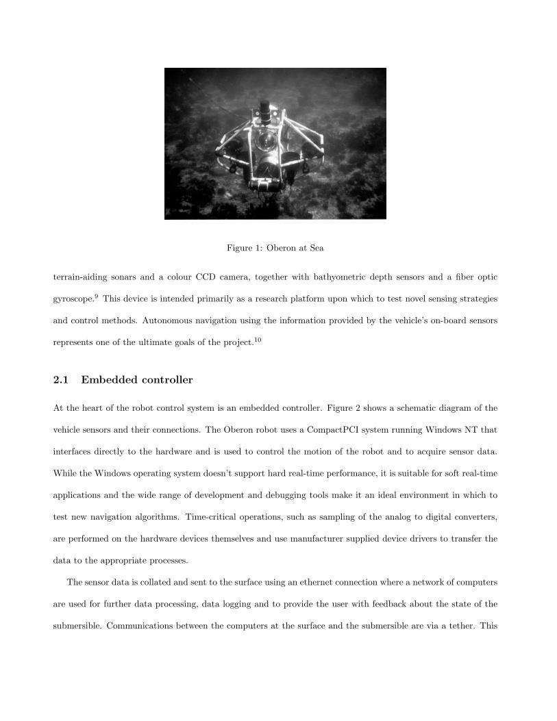
Figure 1: Oberon at Sea

terrain-aiding sonars and a colour CCD camera, together with bathyometric depth sensors and a fiber optic

gyroscope.9 This device is intended primarily as a research platform upon which to test novel sensing strategies

and control methods. Autonomous navigation using the information provided by the vehicle’s on-board sensors

represents one of the ultimate goals of the project.10

2.1 Embedded controller

At the heart of the robot control system is an embedded controller. Figure 2 shows a schematic diagram of the

vehicle sensors and their connections. The Oberon robot uses a CompactPCI system running Windows NT that

interfaces directly to the hardware and is used to control the motion of the robot and to acquire sensor data.

While the Windows operating system doesn’t support hard real-time performance, it is suitable for soft real-time

applications and the wide range of development and debugging tools make it an ideal environment in which to

test new navigation algorithms. Time-critical operations, such as sampling of the analog to digital converters,

are performed on the hardware devices themselves and use manufacturer supplied device drivers to transfer the

data to the appropriate processes.

The sensor data is collated and sent to the surface using an ethernet connection where a network of computers

are used for further data processing, data logging and to provide the user with feedback about the state of the

submersible. Communications between the computers at the surface and the submersible are via a tether. This

Serial

Ethernet

PencilBeam

ScanningSonar

Fan BeamScanning

Sonar

A/D

FiberOptic

Gyroscope

PressureTransducer

D/A8

Cha

nnel

8C

hann

el

ServoMotor

Controller

ServoMotor

Controller

ServoMotor

Controller

ServoMotor

Controller

ServoMotor

Controller

Compass/Tilt

Sensor

SerialSerial

PCI Bus PCI Bus

ColourCCD

Camera

VideoFrame

Grabber

Coaxial Cable

Tether to Surface

Surface Computer Surface Computer

EmbeddedCompactPCI

Figure 2: Vehicle System Diagram

tether also provides power to the robot, a coaxial cable for transmitting video data and a leak detection circuit

designed to shut off power to the vehicle in case water is detected inside the pressure hulls using a pair of optical

diodes.

2.2 Sonar

Sonar is the primary sensor of interest on the Oberon vehicle. There are currently two sonars on the robot. A

Tritech SeaKing imaging sonar has a dual frequency narrow beam sonar head that is mounted on top of the

submersible and is used to scan the environment in which the submersible is operating. It can achieve 360o

scan rates on the order of 0.25 Hz using a pencil beam with a beam angle of 1.8o. This narrow beam allows

the sonar to accurately discriminate bearing returns to objects in the environment. It has a variable mechanical

step size capable of positioning the sonar head to within 0.5o and can achieve range resolution on the order of

50mm depending on the selected scanning range. It has an effective range to 300m allowing for long range target

aquisition in the low frequency mode but can also be used for high definition scanning at lower ranges. The

information returned from this sonar is used to build and maintain a feature map of the environment.

(a) Imagenex Configuration

−1

−0.5

0

0.5−0.5

0

0.5

−0.8

−0.6

−0.4

−0.2

0

0.2

0.4

0.6

x(m)

y(m)z(

m)

rearverticalthruster

horizontalthrusters

Imagenexsonar

SeaKingsonar

foreverticalthrusters

(b) Thrusters

Figure 3: (a) The configuration of the forward looking Imagenex sonar. This placement allows thesonar to ping the altitude as well as search for obstacles in front of the vehicle. (b) The configurationof the vehicle showing the thruster arrangement.

The second sonar is an Imagenex sonar unit operating at 675 kHz and has been mounted at the front of the

vehicle. It is positioned such that its scanning head can be used as a forward and downward looking beam (see

Figure 3). This enables the altitude above the sea floor as well as the proximity of obstacles to be determined

using the wide angle beam of the sonar. The Imagenex sonar features a beam width of 15o x 1.8o allowing a

broad swath to be insonified with each burst of accoustic energy (“ping”) - an ideal sensor for altitude estimation

and obstacle avoidance.

2.3 Internal Sensors

An Andrews Fiber Optic Gyro has been included in the Oberon robot to allow the robot’s orientation to be

determined. This sensor provides the yaw rate and is used to control the heading of the submersible. The bias in

the gyroscope is first estimated while the vehicle is stationery. The bias compensated yaw rate is then integrated

to provide an estimate of vehicle heading. Because the yaw rate signal is noisy, the integration of this signal

causes the estimated heading to drift with time. In addition, the bias can drift as the unit’s internal temperature

changes. Temperature compensation can help to overcome some of these problems and will be considered in

the future. At present, missions do not typically run for longer than 30 minutes and yaw drift does not pose a

significant problem. Subsequent to the data collection presented here, an integrated compass and tilt sensor has

been added to the vehicle. The compass signal is filtered with the output of the gyroscope to estimate the yaw

rate bias of the gyroscope on-line. This will allow the vehicle to undertake longer missions than were previously

feasible. The Simultaneous Localisation and Mapping algorithm to be presented later also allows the yaw rate

bias to be estimated by using tracked features in the environment to provide corrections to errors in the estimated

yaw.

A pressure sensor measures the external pressure experienced by the vehicle. This sensor provides a voltage

signal proportional to the pressure and is sampled by an analogue to digital converter on the embedded controller.

Feedback from this sensor is used to control the depth of the submersible.

2.4 Camera

A colour video camera in an underwater housing is mounted externally on the vehicle. It is used to provide video

feedback of the underwater scenes in which the robot operates. The video signal is transmitted to the surface via

the tether. A Matrox Meteor frame grabber is then used to acquire the video signal for further image processing.

2.5 Thrusters

There are currently 5 thrusters on the Oberon vehicle. Three of these are oriented in the vertical direction while

the remaining two are directed horizontally (see figure 3 (b)). This gives the vehicle the ability to move itself up

and down, control its yaw, pitch and roll and move forwards and backwards. This thruster configuration does not

allow the vehicle to move sideways but this does not pose a problem for the missions envisaged for this vehicle.

3 Vehicle Control System

Control of a mobile robot in six dimensional space in an unstructured, dynamic environment such as is found

underwater can be a daunting and computationally intensive endeavour. Navigation and control both present

difficult challenges in the subsea domain. This section describes the distributed, decoupled control architecture

used to help simplify the controller design for this vehicle.

3.1 Low Level control

The dynamics of the Oberon vehicle are such that the vertical motion of the vehicle is largely decoupled from

the lateral motion. The vehicle is very stable in the roll and and pitch axes due to the large righting moment

induced by the vertical configuration of the pressure vessels. A steel keel provides an added moment to maintain

the vehicle in an upright pose. Two independant PID controllers can therefore be used to control horizontal

and vertical motion of the vehicle. This greatly simplifies the individual controller design. Furthermore, this

particular division of control fits in with many of the anticipated missions to be undertaken by the vehicle. For

example, one of the target missions is to use Oberon to survey an area of the Great Barrier Reef while maintaining

a fixed height above the sea floor.11 The surveying task can then be made independent of maintaining the vehicle

altitude.

The low-level processes run on the embedded controller and are used to interface directly with the hardware

(see figure 4). This allows the controllers to respond quickly to changes in the state of the submersible without

being affected by delays due the data processing and high-level control algorithms running on the remote com-

puters. Set points to the low-level controllers are provided by the behaviours and high-level controllers described

in the next section.

3.2 High-level Controller

The high-level controllers are based on the Distributed Architecture for Mobile Navigation (DAMN).7 DAMN

consists of a group of distributed behaviours sending votes for desirable actions and against objectionable ones

to a centralized command arbiter, which combines these votes to generate actions. The arbiter then provides

-

+

+

++

-

a) Horizontal Low level control

Yaw d

PIDYaw

Output ofYaw

Arbiter

Gyro Yaw RateHorizontalThrusters

Forward Offset d

Output ofFwd

OffsetArbiter

K

Depth d

PIDDepth

Output ofDepthArbiter

PressureSensor

PressureVertical

Thrusters

b) Vertical Low level control

Figure 4: The low level control processes that run on the embedded con-troller. These processes include processes for sampling the internal sensorreadings, computing the PID control outputs and driving the thrusters.

set-points to the low-level controller such that the desired motion is achieved.

Within the framework of DAMN, behaviours must be defined to provide the task-specific knowledge for the

domain. These behaviours operate independently and asynchronously, and each encapsulates the perception,

planning and task execution capabilities necessary to achieve one specific aspect of robot control, and receives

only the data specifically required for that task.12

The raw sensor data is preprocessed to produce information that is of interest to multiple behaviours designed

to control the vehicle’s actions. These preprocessors act as virtual sensors by providing data for the behaviours

that is abstracted from the raw sensor data, simplifying the individual behaviour design. The behaviours monitor

the outputs of the relevant virtual sensors and determine the optimal action to achieve the behaviour’s objectives.

The behaviours send votes to the arbiters which combine the votes in the system to determine the action which will

allow the system to best achieve its goals. A task-level mission planner is used to enable and disable behaviours

in the system depending on the current state of the mission and its desired objectives. A command arbitration

process combines the votes from the behaviours and selects the optimal action to satisfy the goals of the system.

In the present implementation, two arbiters are used to provide set-points to the low-level controllers. One

arbiter is responsible for setting the desired depth of the vehicle while the other sets the desired yaw and

forward offset to achieve horizontal motion. The behaviours are consequently divided into horizontal and vertical

behaviours.

For a survey mission, the vertical behaviours are responsible for keeping the submersible from colliding with

the sea floor. The vertical behaviours that run on the vehicle include maintain minimum depth, maintain

minimum altitude, maintain depth and maintain altitude. The combination of the outputs of these behaviours

determines the depth at which the vehicle will operate. A large negative vote by the maintain minimum altitude

behaviour, for example, will keep the vehicle at a minimum distance from the sea floor.

The horizontal behaviours that run during a typical survey mission include follow line (using sonar and/or

vision), avoid obstacles, move to a location and perform survey. The combination of the outputs of these

behaviours determines the orientation maintained by the vehicle as well as the forward offset applied to the two

horizontal thrusters. This allows the vehicle to move forward while maintaining its heading.

A schematic repsentation of the control structure of the Oberon vehicle is shown in figure 5. The vertical

behaviours rely primarily on the depth sensor whereas the horizontal behaviours use vision, gyro and the imaging

sonar (Tritech SeaKing). The forward look sonar (Imagenex) is shared between both horizontal and vertical

behaviours. It is used to provide periodic altitude measurements for the maintain altitude behaviour while

providing an indication as to the presence of obstacles in front of the vehicle to the obstacle avoidance behaviour.

A task scheduler that allow resources to be shared between various tasks is used to allocate this sensor to the

two behaviours. Clearly, tasks that are deemed more important to the accomplishment of the vehicle’s mission

need to be given preferential access to the resources they require. For example, the altitude task is allowed to

ping the bottom in preference to the avoid obstacles behaviour since the AUV typically operates at relatively low

speeds and collision with the bottom is more of a concern than collision with obstacles in front of the vehicle.

SurveyArea

Raw PingsRange/Bearing

dYaw

ImagingSonar

Gyro

SLAMFeature

Extraction

PressureSensor

Altitude

ForwardLookSonar

Proximity toObstacle

MinimumAltitude

MaintainAltitude

MaintainDepth

AvoidObstacle

FollowLine

MinimumDepth

DepthArbiter

YawArbiter

Yaw Votes/Fwd Offset

Votes

Depth Votes

Yaw dFwdOffset d

Depth d

VisionLine

TrackingVideo Orientation of Line

MoveToPosition

Depth

Altitude

Obstacle Distance

PositionEstimates

Sensors Virtual Sensors Behaviours Arbiters

Commands Sent toLow LevelControllers

Commands Sent toLow LevelControllers

MissionPlanner

Depth

Figure 5: The high level process and behaviours that run the vehicle. The sensor data is pre-processedto produce virtual sensor information available to the behaviours. The behaviours receive the virtualsensor information and send votes to the arbiters who send control signals to the low level controllers.The greyed out boxes are the SLAM processes that will be detailed in section 4.

3.3 Distributed control

The control structure described in the previous sections is implemented using a distributed control strategy. A

number of processes have been developed to accomplish the tasks of gathering data from the robot’s sensors,

processing this data and reasoning about the course of action to be taken by the robot. These processes are

distributed across a network of computers and communicate asynchronously via a TCP/IP socket-based interface

using a message passing protocol developed at the Centre.

A central communications hub is responsible for routing messages between the distributed processes running

on the vehicle and on the command station. Processes register their interest in messages being sent by other

processes in the system and the hub routes the messages when they arrive. While this communications structure

has some drawbacks, such as potential communications bottlenecks and reliance on the performance of the central

hub, it does provide some interesting possibilities for flexible configuration, especially during the development

TCP/IP

TCP/IP

TCP/IP TCP/IP

TCP/IP

TCP/IP

TCP/IP

BaseGUI

Sea KingGUI

Sea KingFeature

Extractor

Sea KingSlam

Sea KingRemote

OberonLow Level

DataLogger

Sea KingSonar

RS-232

A/D

Gyro

D/A

Thrusters

____________________________ TCP/IP

ImagenexRemote

ImagenexSonar

RS-232

BaseComm

Pressure

(a) Vehicle controller

TCP/IP

TCP/IP

TCP/IP TCP/IP

TCP/IP

TCP/IP

BaseGUI

Sea KingGUI

Sea KingFeature

Extractor

Sea KingSlam

DataPlayback

DataLogger Base

Comm

____________________________

(b) Data Playback

TCP/IP

TCP/IP

TCP/IP TCP/IP

TCP/IP

TCP/IP

BaseGUI

Sea KingGUI

Sea KingFeature

Extractor

Sea KingSlam

OberonSimulation

DataLogger Base

Comm

____________________________

(c) Simulation

Figure 6: a) The low-level processes that control the vehicle can easily be replaced by b) a dataplayback process to replay mission data or by c) a simulator to develop closed-loop control algorithmsprior to vehicle deployment.

cycle of the system. In the context of the low information rates present in an underwater vehicle, the system

performs well. The implementation also allow for easy system development. For example, as shown in Figure

6, the low-level processes that control the vehicle can easily be replaced by a data playback process to replay

mission data or by a simulator. This enables the development of closed-loop control algorithms prior to vehicle

deployment.

The control architecture presented here provides a distributed environment in which to control the robot.

Processes can be developed and added to the system without major changes to the overall architecture. New

mission-dependent behaviours can be introduced without requiring changes to the rest of the controller. The

communications have also been abstracted away from the operation of the various processes. This provides

the potential to change the inter-process communications medium without necessitating major changes to the

behaviours themselves.

4 Position Estimation

Many of the behaviours in the system rely on the ability of the vehicle to estimate its position. Behaviours such as

move to position and avoid obstacles need to have a reliable estimate of the vehicle position in order to function

correctly. While many land-based robots use GPS or maps of the environment to provide accurate position

updates, a robot navigating underwater does not have access to this type of information. In typical underwater

scientific missions, a-priori maps are seldom available.13 This section presents the feature based localisation and

mapping technique used for generating vehicle position estimates.

4.1 The Estimation Process

The localisation and map building process consists of a recursive, three-stage procedure comprising prediction,

observation and update steps using an Extended Kalman Filter (EKF).2 The EKF estimates the two dimensional

pose of the vehicle xv, made up of the position (xv, yv) and orientation ψv, together with the estimates of the

positions of the N landmarks xi, i = 1...N , using the observations from the sensors on board the submersible.

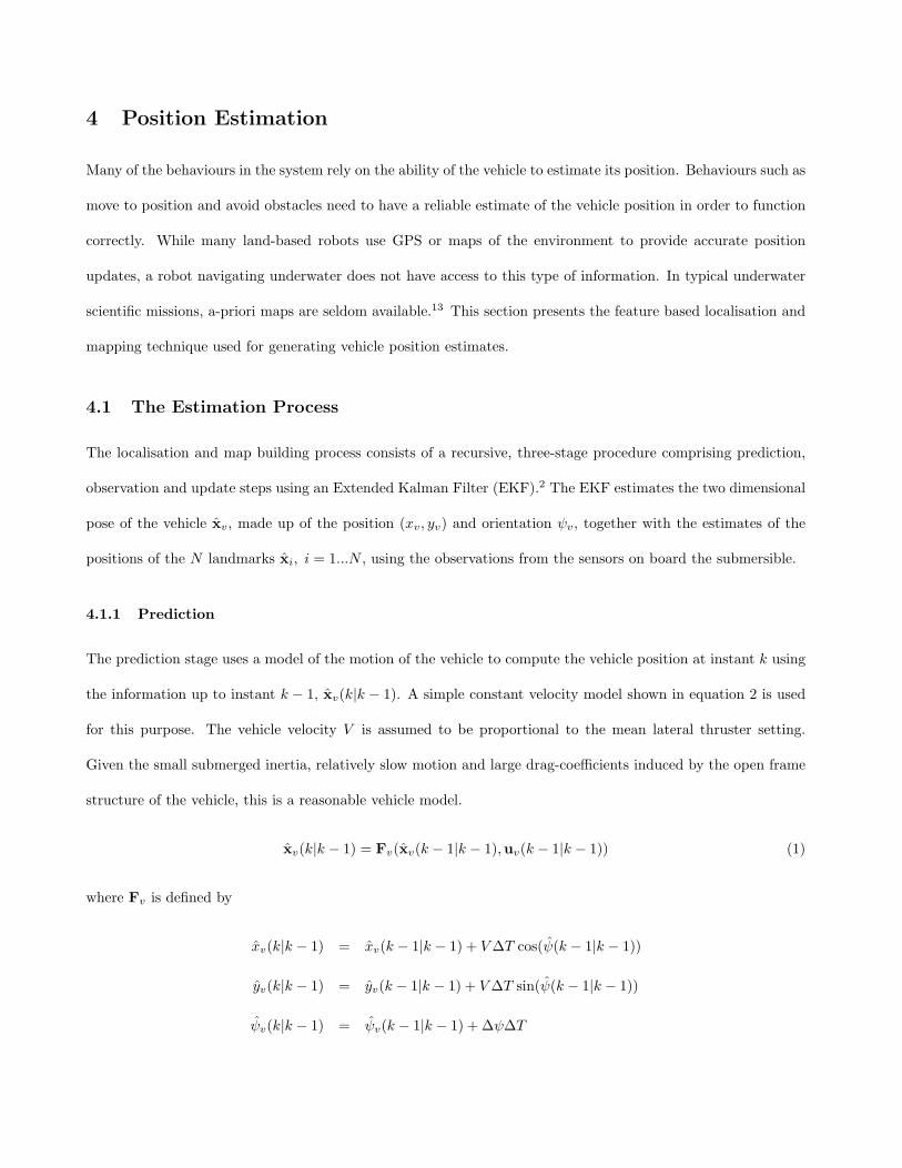
4.1.1 Prediction

The prediction stage uses a model of the motion of the vehicle to compute the vehicle position at instant k using

the information up to instant k − 1, xv(k|k − 1). A simple constant velocity model shown in equation 2 is used

for this purpose. The vehicle velocity V is assumed to be proportional to the mean lateral thruster setting.

Given the small submerged inertia, relatively slow motion and large drag-coefficients induced by the open frame

structure of the vehicle, this is a reasonable vehicle model.

xv(k|k − 1) = Fv(xv(k − 1|k − 1), uv(k − 1|k − 1)) (1)

where Fv is defined by

xv(k|k − 1) = xv(k − 1|k − 1) + V∆T cos(ψ(k − 1|k − 1))

yv(k|k − 1) = yv(k − 1|k − 1) + V∆T sin(ψ(k − 1|k − 1))

ψv(k|k − 1) = ψv(k − 1|k − 1) + ∆ψ∆T

Table 1: SLAM filter parametersSampling period ∆T 0.1sVehicle X process noise std dev σx 0.075mVehicle Y process noise std dev σy 0.075mVehicle heading process noise std dev σψ 0.5o

Vehicle velocity std dev σv 0.75m/sVehicle steering std dev σdψ 0.5o

Gyro/Compass std dev σc 0.5o

Range measurement std dev σR 0.5mBearing measurement std dev σB 2.0o

Sonar range 15mSonar resolution 0.075m

The covariance of the vehicle and feature states, P(k|k), are predicted using the non-linear state prediction

equation. The predicted covariance is computed using the gradient of the state propagation equation, ∇Fv,

linearised about the current estimate, the process noise model, Q, and the control noise model, U. The filter

parameters used in this application are shown in table 1.

P(k|k − 1) = ∇FvP(k − 1|k − 1)∇FTv +∇FvU(k|k − 1)∇FT

v +Q(k|k − 1) (2)

with

Q(k|k − 1) = diag

[σ2

x σ2y σ2

ψ

](3)

and

U(k|k − 1) = diag

[σ2

v σ2dψ

](4)

4.1.2 Observation

Observations are made using an imaging sonar that scans the horizontal plane around the vehicle. Point features

are extracted from the sonar scans and are matched against existing features in the map. The feature matching

algorithm will be described in more detail in Section 4.2. The observation consists of a relative distance and

orientation from the vehicle to the feature. The predicted observation, zi(k|k− 1), when observing landmark “i”

located at xi can be computed using the non-linear observation model Hi(xv(k|k − 1), xi(k|k − 1)).

zi(k|k − 1) = Hi(xv(k|k − 1), xi(k|k − 1)) (5)

where Hi is defined by

ziR(k|k − 1) =√(xv(k|k − 1)− xi(k|k − 1))2 + (yv(k|k − 1)− yi(k|k − 1))2

ziθ(k|k − 1) = arctan((yv(k|k − 1)− yi(k|k − 1))(xv(k|k − 1)− xi(k|k − 1)))− ψv(k|k − 1)

(6)

The difference between the actual observation z(k|k − 1) and the predicted observation z(k|k − 1) is termed the

innovation ν(k|k − 1).

νi(k|k − 1) = zi(k|k − 1)− zi(k|k − 1) (7)

The innovation covariance S(k|k − 1) is computed using the current state covariance estimate P(k|k − 1), the

gradient of the observation model, ∇H(k|k − 1) and the covariance of the observation model R(k|k − 1).

S(k|k − 1) = ∇H(k|k − 1)P(k|k − 1)∇H(k|k − 1)T +R(k|k − 1) (8)

with

R(k|k − 1) = diag

[σ2

R σ2B

](9)

4.1.3 Update

The state estimate can now be updated using the optimal gain matrix W(k). This gain matrix provides a

weighted sum of the prediction and observation and is computed using the innovation covariance, S(k|k − 1)

and the predicted state covariance, P(k|k − 1). This is used to compute the state update x(k|k) as well as the

updated state covariance P(k|k).

x(k|k) = x(k|k − 1) +W(k|k − 1)ν(k|k − 1) (10)

P(k|k) = P(k|k − 1)− W(k|k − 1)S(k|k − 1)W(k|k − 1)T (11)

where

W(k|k − 1) = P(k|k − 1)∇H(k|k − 1)S−1(k|k − 1) (12)

4.2 Feature Extraction for Localisation

The development of autonomous map based navigation relies on the ability of the system to extract appropriate

and reliable features with which to build maps.14,15 Point features are identified from the sonar scans returned

by the imaging sonar and are used to build up a map of the environment. The extraction of point features from

the sonar data is essentially a three stage process. The range to the principal return must first be identified in

individual pings. This represents the range to the object that has produced the return. This is complicated by

such issues as multiple and/or specular reflections, problems which are seen in the pool but less so in a natural

environment. The principal returns must then be grouped into clusters. Small, distinct clusters can be identified

as point features and the range and bearing to the target estimated. Finally, the range and bearing information

must be matched against existing features in the map.

Sonar targets are currently introduced into the environment in which the AUV will operate (see Figure 7)

in order to obtain identifiable and stable features. A prominent portion of the reef wall or a rocky outcropping

might also be classified as a point feature. If the naturally occurring point features are stable they will also be

incorporated into the map. Development of techniques to extract more complex natural features, such as coral

reefs and natural variations on the sea floor, is an area of active research as this will allow the submersible to be

deployed in a larger range of natural environments without the need to introduce artificial beacons.

The sonar targets produce strong sonar returns that can be charaterised as point targets for the purposes of

mapping (see Figure 8). The lighter sections in the scan indicate stronger intensity returns. As can be seen from

the figure, the pool walls act as specular reflectors causing a considerable amount of additional sonar noise as

well as multiple reflections that appear to be objects ‘behind’ the walls.

The three stages of feature extraction are described in more detail in the following subsections.

4.2.1 Principal Returns

The data returned by the SeaKing sonar consists of the complete time history of each sonar ping in a discrete

set of bins scaled over the desired range. The first task in extracting reliable features is to identify the principal

return from the ping data. The principal return is considered to be the start of the maximum energy component

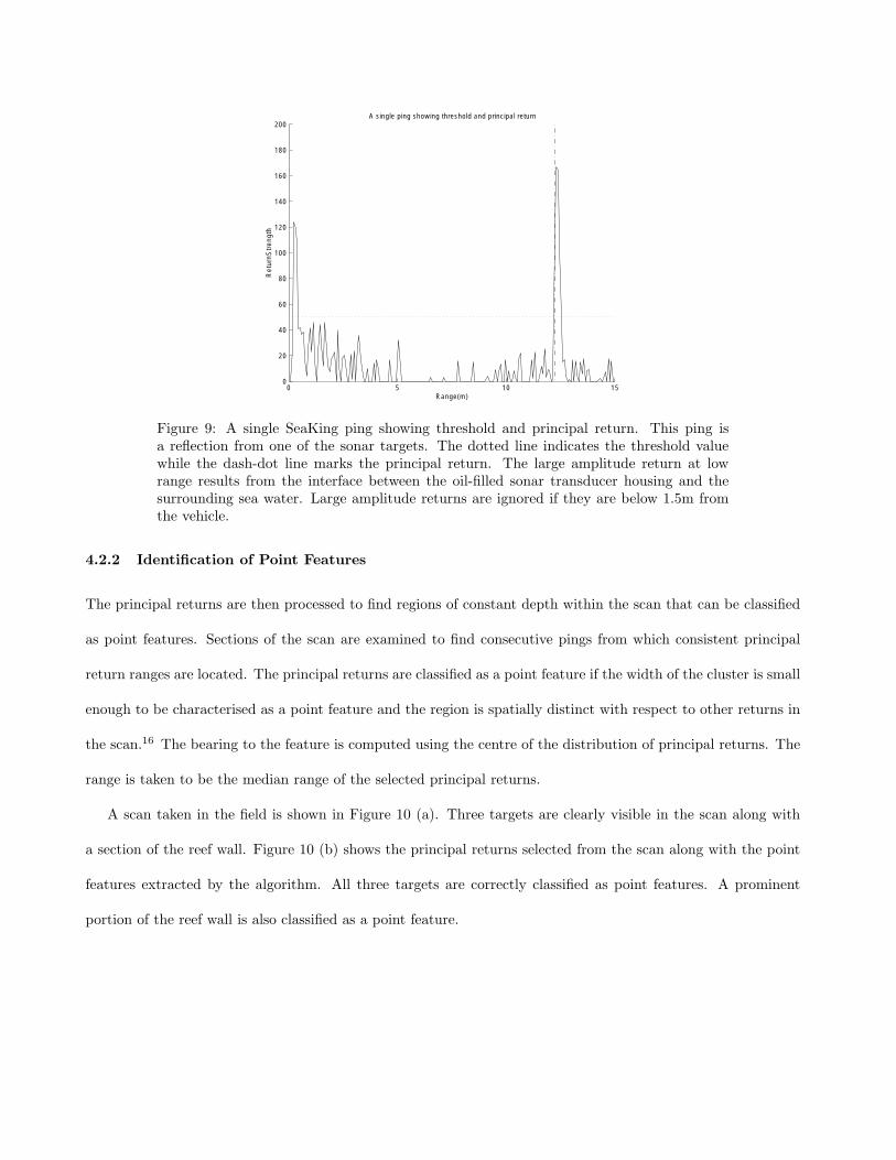
of the signal above a certain noise threshold. Figure 9 shows a single ping taken from a scan in the field. This

Figure 7: An image captured from the submersible of one of the sonar targets deployed atthe field test site.

Figure 8: Scan in the pool showing sonar targets

return is a reflection from one of the sonar targets and the principal return is clearly visible. The return exhibits

very good signal to noise ratio making the extraction of the principal returns relatively straightforward.

0 5 10 150

20

40

60

80

100

120

140

160

180

200A single ping showing threshold and principal return

Range(m)

Ret

urnS

tren

gth

Figure 9: A single SeaKing ping showing threshold and principal return. This ping isa reflection from one of the sonar targets. The dotted line indicates the threshold valuewhile the dash-dot line marks the principal return. The large amplitude return at lowrange results from the interface between the oil-filled sonar transducer housing and thesurrounding sea water. Large amplitude returns are ignored if they are below 1.5m fromthe vehicle.

4.2.2 Identification of Point Features

The principal returns are then processed to find regions of constant depth within the scan that can be classified

as point features. Sections of the scan are examined to find consecutive pings from which consistent principal

return ranges are located. The principal returns are classified as a point feature if the width of the cluster is small

enough to be characterised as a point feature and the region is spatially distinct with respect to other returns in

the scan.16 The bearing to the feature is computed using the centre of the distribution of principal returns. The

range is taken to be the median range of the selected principal returns.

A scan taken in the field is shown in Figure 10 (a). Three targets are clearly visible in the scan along with

a section of the reef wall. Figure 10 (b) shows the principal returns selected from the scan along with the point

features extracted by the algorithm. All three targets are correctly classified as point features. A prominent

portion of the reef wall is also classified as a point feature.

(a) Field Scan

−15 −10 −5 0 5 10 15−15

−10

−5

0

5

10

15Sea King Feature Extraction

X (m)Y

(m

)

(b) Extracted Features

Figure 10: (a) a scan in the field showing sonar targets (b) the principal returns (+) and the extractedpoint features (�) from the scan in (a)

4.2.3 Feature Matching

Once a point feature has been extracted from a scan, it must be matched against known targets in the environ-

ment. A two-step matching algorithm is used in order to reduce the number of targets that are added to the

map (see Figure 11).

When a new range and bearing observation is received from the feature extraction process, the estimated

position of the feature is computed using the current estimate of vehicle position. This position is then compared

with the estimated positions of the features in the map using the Mahanabolis distance.2 If the observation can

be associated to a single feature the EKF is used to generate a new state estimate. An observation that can be

associated with multiple targets is rejected since false observations can destroy the integrity of the estimation

process.

If the observation does not match to any targets in the current map, it is compared against a list of tentative

targets. Each tentative target maintains a counter indicating the number of associations that have been made

with the feature as well as the last observed position of the feature. If a match is made, the counter is incremented

Reject multiple featurematches to avoid

corrupting the map

Pass Range Bearingobservation to filteralong with matched

feature index

Add a new tentativefeature to the list

No

Add a new feature tothe map and removethe current tentativefeature from the list.

New Range/Bearing to

feature received

Match to tentativefeature list?

Match to feature in the map?

Match multiplefeatures in map?

Is Count > threshold?

Update position andincrement match count

YesYes

Yes

Yes

No

No

Figure 11: The feature matching algorithm

and the observed position is updated. When the counter passes a threshold value, the feature is considered to

be sufficiently stable and is added to the map. If the potential feature cannot be associated with any of the

tentative features, a new tentative feature is added to the list. Tentative features that are not reobserved are

removed from the list after a fixed time interval has elapsed.

5 Experimental Results

Oberon was deployed in a number of environments including the pool at the University of Sydney and in a natural

terrain environment along Sydney’s coast, in order to evaluate the control and mapping techniques developed in

the previous sections. This section presents the results obtained.

5.1 Decoupled Control

This section describes the performance of the vertical control behaviours. These behaviours allow the vehicle to

navigate without risk of hitting the sea floor.

0 100 200 300 400 500 600 7000

1

2

3

Time (s)

Alti

tude

(m)

Altitude, Depth & Thruster Output vs time

0 100 200 300 400 500 600 700−6

−4

−2

0

Time (s)

Dep

th (

m)

0 100 200 300 400 500 600 700−100

−50

0

50

100

Time (s)

Thr

uste

r S

ettin

g(%

)

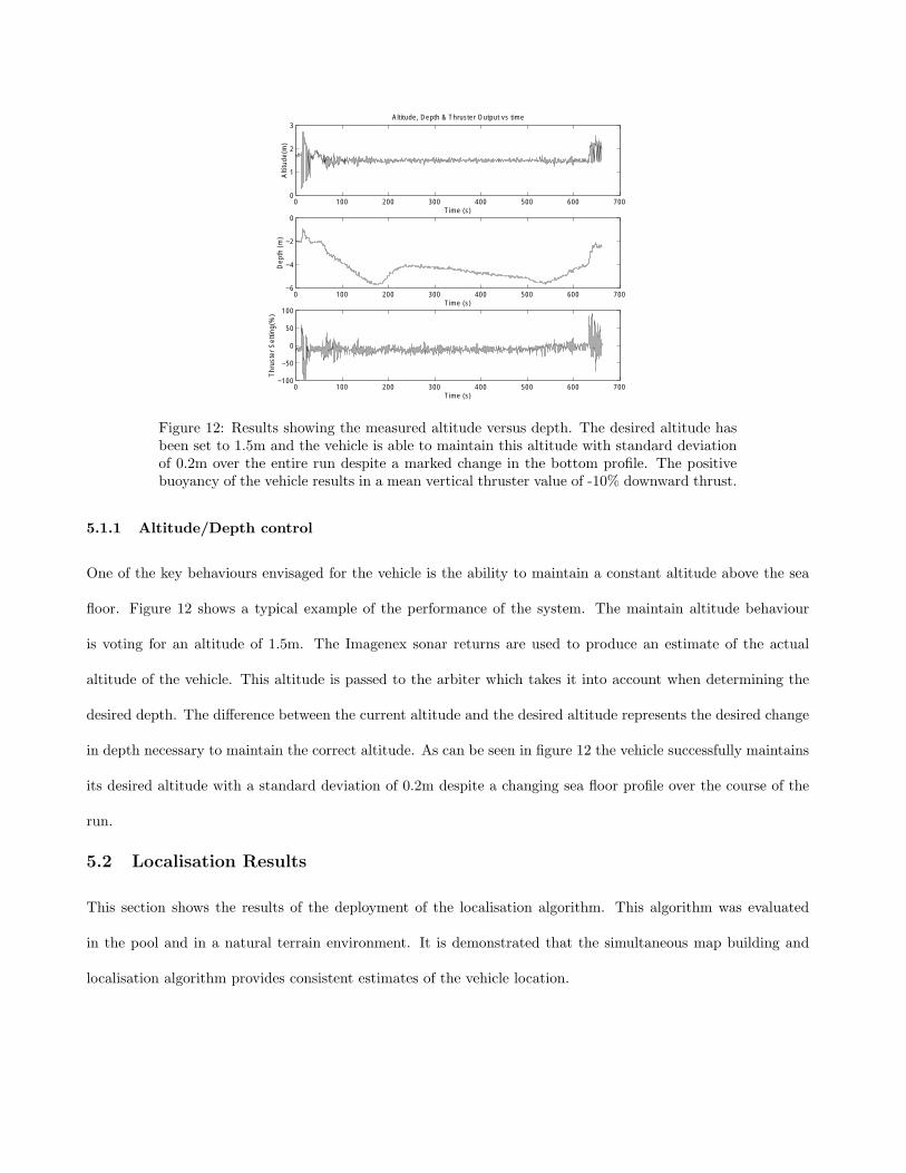
Figure 12: Results showing the measured altitude versus depth. The desired altitude hasbeen set to 1.5m and the vehicle is able to maintain this altitude with standard deviationof 0.2m over the entire run despite a marked change in the bottom profile. The positivebuoyancy of the vehicle results in a mean vertical thruster value of -10% downward thrust.

5.1.1 Altitude/Depth control

One of the key behaviours envisaged for the vehicle is the ability to maintain a constant altitude above the sea

floor. Figure 12 shows a typical example of the performance of the system. The maintain altitude behaviour

is voting for an altitude of 1.5m. The Imagenex sonar returns are used to produce an estimate of the actual

altitude of the vehicle. This altitude is passed to the arbiter which takes it into account when determining the

desired depth. The difference between the current altitude and the desired altitude represents the desired change

in depth necessary to maintain the correct altitude. As can be seen in figure 12 the vehicle successfully maintains

its desired altitude with a standard deviation of 0.2m despite a changing sea floor profile over the course of the

run.

5.2 Localisation Results

This section shows the results of the deployment of the localisation algorithm. This algorithm was evaluated

in the pool and in a natural terrain environment. It is demonstrated that the simultaneous map building and

localisation algorithm provides consistent estimates of the vehicle location.

5.2.1 Swimming Pool Trials

During tests in the pool at the University of Sydney, six sonar targets were placed in the pool such that these form

a circle roughly 6m in diameter in the area in which the submersible is operating. The vehicle starts to the left of

the target cluster and is driven in a straight line perpendicular to the pool walls over a distance of approximately

5m. The submersible is then driven backwards over the same distance and returns to the initial position. A PID

controller maintains the heading of the submersible using feedback from a fiber optic gyro. During the short

duration of the trials, the accumulated drift in the gyro orientation estimate is considered negligible. Forward

thrust is achieved by adding a common voltage to each thruster amplifier control signal.11

The distance to the pool walls measured with the sonar is used to determine the true position of the submersible

in the pool. The walls are clearly evident in the scans taken in the pool giving us a good approximation of the

actual position of the submersible.

Figure 13 shows the position estimate along the axis perpendicular to one of the pool walls generated by

SLAM during one of the runs in the pool. These results show that the robot is able to successfully determine its

position relative to the walls of the pool despite the effect of the tether, which tends to dominate the dynamics

of the vehicle at low speeds. With the low thruster setting, the AUV stops after it has traversed approximately

4.5m, with the catenary created by the deployed tether overcoming the forward thrust created by the vehicle’s

thrusters. The SLAM algorithm is able to determine the fact that the vehicle has stopped using observations

from its feature map.

The error in the perpendicular position relative to the pool walls is plotted along with the 95% confidence

bounds in Figure 14. While the estimated error bounds are conservative, this allows the optimal estimator to

account for environmental disturbances in the field such as current and the forces exerted by the tether catenary.

In order to test the filter consistency, the innovation sequences can be checked against the innovation covari-

ance estimates. This is the only method available to monitor on-line filter performance when ground truth is

unavailable. As can be seen in Figure 15, the innovation sequences for range and bearing are consistent.

The error in the estimated position of the beacons can be plotted against their respective 95% confidence

bounds. This is shown in Figure 16 for Beacon 2 which was seen from the start of the run and Figure 17 for

0 50 100 150 200 250 300 350 400 450 500−4

−2

0

2

4

6

8

10Actual Position vs Estimated Position along 1D axis of motion

time(s)

x(m

)

Figure 13: Position of the robot in the pool along the 1D axis of motion. The estimate isthe solid line, the true position is the dash-dot line while the error bounds are shown asthe dotted lines. The gap in the results in the middle of the trial between 220-320 secondsoccurred when the vehicle forward motion was stopped and the data logging turned off.The data logging was resumed before the vehicle began moving back towards its initialposition.

0 50 100 150 200 250 300 350 400 450 500−4

−3

−2

−1

0

1

2

3

4Actual position error vs 95% confidence bounds

t(s)

Err

or (

m)

Figure 14: The 95% confidence bounds com-puted using the covariance estimate for theerror in the X estimate compared to the ac-tual error relative to the pool walls.

0 50 100 150 200 250 300 350 400−3

−2

−1

0

1

2

3Range Innovation with 95% confidence bounds

Time (s)

Ran

ge In

nova

tion

(m)

0 50 100 150 200 250 300 350 400−1

−0.5

0

0.5

1Bearing Innovation with 95% confidence bounds

Time (s)

Bea

ring

Inno

vatio

n (r

ad)

Figure 15: The range and bearing innova-tion sequences plotted against their 95% con-fidence bounds. The innovation is plotted asa solid line while the confidence bounds arethe dash-dot lines.

Beacon 4 which is only incorporated into the map after the first minute.

The final map generated by the SLAM algorithm is plotted in Figure 18. The true position of the sonar

targets is shown and the associated map features can clearly be seen in the final map estimates. A number of

0 50 100 150 200 250 300 350 400 450−5

0

5Beacon 2 Position Estimate errors in X with Standard Deviation

time (s)

Err

or in

X (

m)

0 50 100 150 200 250 300 350 400 450−5

0

5Beacon 2 Position Estimate errors in Y with Standard Deviation

time (s)

Err

or in

Y (

m)

Figure 16: The Error in the estimated X andY positions for Beacon 2 along with the 95%confidence bounds. This shows that the bea-con location estimate is consistent.

0 50 100 150 200 250 300 350 400 450−5

0

5Beacon 4 Position Estimate errors in X with Standard Deviation

time (s)

Err

or in

X (

m)

0 50 100 150 200 250 300 350 400 450−5

0

5Beacon 4 Position Estimate errors in Y with Standard Deviation

time (s)

Err

or in

Y (

m)

Figure 17: The Error in the estimated X andY positions for Beacon 4 along with the 95%confidence bounds. This shows that the bea-con location estimate is consistent.

point features have also been identified along the pool wall to the left of the image. The estimated path of the

submersible is shown along with the covariance ellipses describing the confidence in the estimate. It is clear that

the covariance remains fairly constant throughout the run.

5.2.2 Field Trials

The SLAM algorithms have also been tested during deployment in a natural environment off the coast of Sydney.

The submersible was deployed in a natural inlet with the sonar targets positioned in a straight line in intervals of

10m. Since there is currently no absolute position sensor on the vehicle, the performance of the positioning filter

cannot be measured against ground truth at this time. The innovation sequence can, however, be monitored to

check the consistency of the estimates. Figure 19 shows that the innovation sequences are within the covariance

bounds computed by the algorithm.

The plot of the final map shown in Figure 20 clearly shows the position of the sonar feature targets along with

a number of tentative targets that are still not confirmed as sufficiently reliable. Some of the tentative targets are

from the reef wall while others come from returns off of the tether. These returns are typically not very stable

and therefore do not get incorporated into the SLAM algorithm. The sonar principal returns have been plotted

relative to the estimated position of the vehicle. The reef wall to the right of the vehicle and the end of the inlet

−4 −2 0 2 4 6 8 10

−6

−5

−4

−3

−2

−1

0

1

2

3

4

1

2

3

4

5

6

Slam position of features in pool

X(m)

Y(m

Sonar Returns Tentative Features Map Features True Beacon PositionVehicle Path

Figure 18: Path of the robot shown against the final map of the environment. The es-timated position of the features are shown as circles with the covariance ellipses showingtheir 95% confidence bounds. The true positions are plotted as ’*’. Tentative targets thathave not yet been added to the map are shown as ’+’. The robot starts at (0,0) andtraverses approximately 5m in the X direction before returning along the same path in thereverse direction.

0 50 100 150 200 250 300−3

−2

−1

0

1

2

3Range Innovation with 95% confidence bounds

Time (s)

Ran

ge In

nova

tion

(m)

0 10 20 30 40 50 60−1

−0.5

0

0.5

1Bearing Innovation with 95% confidence bounds

Time (s)

Bea

ring

Inno

vatio

n (r

ad)

Figure 19: The range and bearing innovation sequences plotted against their 95% confi-dence bounds. The innovation is plotted as a solid line while the confidence bounds arethe dash-dot lines.

−30 −20 −10 0 10 20 30

−35

−30

−25

−20

−15

−10

−5

0

5

X (m)

Y (

m)

Estimated Path of the VehicleSonar Returns Tentative FeaturesMap Features Vehicle Path

Figure 20: Path of robot shown against final map of the environment. The estimatedposition of the features are shown as circles with the covariance ellipses showing their95% confidence bounds. Tentative targets that have not yet been added to the map areshown as ’+’. The series of tentative targets to the right of the image occur from thereef wall. The natural point features tend not to be very stable, though, and are thus notincorporated into the map.

are clearly visible.

6 Summary and Conclusions

In this paper, it has been shown that the decoupled, distributed control architecture proposed here is practically

feasible for the control of an underwater vehicle. During deployment in a natural terrain environment on Sydney’s

shore-line, these control schemes have proven to be effective in controlling the motion of the submersible. Given

the nature of the anticipated missions for this vehicle, it appears that more complicated control schemes relying

on complex models of the submersible dynamics are not necessary in the context of this problem.

It has also been shown that SLAM is practically feasible in both a swimming pool at the University of Sydney

and in a natural terrain environment on Sydney’s shore-line. By using terrain information as a navigational aid,

the vehicle is able to detect unmodeled disturbances in its motion induced by the tether drag and the effect of

currents.

The focus of future work is on representing natural terrain in a form suitable for incorporation into the SLAM

algorithm. This will enable the vehicle to be deployed in a broader range of environments without the need to

introduce artificial beacons. Another outstanding issue is that of map management. As the number of calculations

required to maintain the state covariance estimates increases with the square of the number of beacons in the

map, criteria for eliminating features from the map as well as for partitioning the map into submaps becomes

important. This is especially true for longer missions in which the number of available landmarks is potentially

quite large. Finally, integration of the localisation and map building with mission planning is under consideration.

This will allow decisions concerning sensing strategies to be made in light of the desired mission objectives.

References

[1] JA Castellanos, JMM Montiel, J Neira, JD Tardos. “Sensor Influence in the Performance of Simultaneous

Mobile Robot Localization and Map Building”. 6th International Symposium on Experimental Robotics. pp

203-212, Sydney, NSW, Australia, 1999

[2] MWMG Dissanayake, P Newman, HF Durrant-Whyte, S Clark, M Csorba. “An Experimental and The-

oretical Investigation into Simultaneous Localisation and Map Building”. 6th International Symposium on

Experimental Robotics. pp 171-180, Sydney, NSW, Australia, 1999

[3] HJS Feder, JJ Leonard, CM Smith. “Adaptive sensing for terrain aided navigation”. IEEE Oceanic Engineer-

ing Society. OCEANS’98. pp.336-41 vol.1. New York, NY, USA, 1998

[4] JJ Leonard, HF Durrant-Whyte, “Simultaneous Map Building and Localisation for an Autonomous Mobile

Robot”, IEEE/RSJ International Workshop on Intelligent Robots and Systems IROS ’91, pp.1442-1447, New

York, NY, USA, 1991

[5] WD Rencken “Concurrent localisation and map building for mobile robots using ultrasonic sensors”. Pro-

ceedings of the 1993 IEEE/RSJ International Conference on Intelligent Robots and Systems, pp.2192-7 vol.3.

New York, NY, USA, 1993

[6] L Whitcomb, D Yoerger, H Singh, Mindell, “Towards Precision Robotic Maneuvering, Survey, and Manip-

ulation in Unstructured Undersea Environments”, Robotics Research - The Eight International Symposium,

pp. 346-353, Springer-Verlag, London 1998

[7] J Rosenblatt “The Distributed Architecture for Mobile Navigation”. Journal of Experimental and Theoretical

Artificial Intelligence, vol.9 no.2/3 pp.339-360, April-September, 1997

[8] J Rosenblatt, S Williams, HF Durrant-Whyte “Behavior-Based Control for Autonomous Underwater Explo-

ration” In proceedings of IEEE International Conference on Robotics and Automation (ICRA00) pp.1793-

1798, San Francisco, CA, 2000

[9] S Williams, P Newman, G Dissanayake, HF Durrant-Whyte “Autonomous Underwater Simultaneous Localisa-

tion and Mapping” In proceedings of IEEE International Conference on Robotics and Automation (ICRA00),

pp.920-925, San Francisco CA, 2000

[10] P Newman and HF Durrant-Whyte, “Toward Terrain-Aided Navigation of a Subsea Vehicle”, FSR’97 In-

ternational Conference on Field and Service Robotics, pp.244-248, Canberra, Australia, 1997.

[11] S Williams, P Newman, S Majumder, J Rosenblatt, HF Durrant-Whyte , “Autonomous Transect Survey-

ing of the Great Barrier Reef”, Australian Conference on Robotics and Automation (ACRA’99), pp. 16-20

Brisbane, QLD, 1999.

[12] RA Brooks. “A robust, layered control system for a mobile robot”. IEEE Journal of Robotics and Automation,

vol.RA-2, no.1 , pp 14-23 April, 1986

[13] L Whitcomb, D Yoerger, H Singh, J Howland, “Advances in Underwater Robot Vehicles for Deep Ocean

Exploration: Navigation, Control and Survey Operations”, 9th Internation Symposium on Robotics Research

(ISRR’99), pp. 346-353, Snowbird, Utah, USA, 1999

[14] R Bauer, WD Rencken. “Sonar feature based exploration”. 1995 IEEE/RSJ International Conference on

Intelligent Robots and Systems.pp.148-53 vol.1. Los Alamitos, CA, USA, 1995

[15] JJ Leonard, RN Carpenter, HJS Feder, “Stochastic Mapping Using Forward Look Sonar”, FSR ’99 Inter-

national Conference on Field and Service Robotics , pp.69-74, Pittsburg, PA, USA 1999

[16] P Newman, “On The Structure and Solution of the Simultaneous Localisation and Map Building Problem”,

PhD Thesis, University of Sydney, 1999