Autonomic Wireless Networking

Autonomic Wireless Networking

Doctoral thesis

Héctor Luis Velayos Muñoz

Laboratory for Communication Networks Department of Signals, Sensors and Systems

KTH Royal Institute of Technology Stockholm, Sweden

May 2005


A dissertation submitted to KTH, Royal Institute of Technology for the Doctor of Philosophy degree

2005 Héctor Luis Velayos Muñoz KTH Royal Institute of Technology Department of Signals, Sensors and Systems Laboratory for Communication Networks SE-100 44 Stockholm, Sweden

TRITA-S3-LCN-0505 ISSN 1653-0837 ISRN KTH/S3/LCN/--05/05--SE

Printed in 100 copies by Universitetsservice US AB, Stockholm 2005

1

ABSTRACT Large-scale deployment of IEEE 802.11 wireless LANs (WLANs) remains a

significant challenge. Many access points (APs) must be deployed and interconnected without a-priori knowledge of the demand. We consider that the deployment should be iterative, as follows. At first, access points are deployed to achieve partial coverage. Then, usage statistics are collected while the network operates. Overloaded and under-utilized APs would be identified, giving the opportunity to relocate, add or remove APs. In this thesis, we propose extensions to the WLAN architecture that would make our vision of iterative deployment feasible.

One line of work focuses on self-configuration, which deals with building a WLAN from APs deployed without planning, and coping with mismatches between offered load and available capacity. Self-configuration is considered at three levels. At the network level, we propose a new distribution system that forms a WLAN from a set of APs connected to different IP networks and supports AP auto-configuration, link-layer mobility, and sharing infrastructure between operators. At the inter-cell level, we design a load-balancing scheme for overlapping APs that increases the network throughput and reduces the cell delay by evenly distributing the load. We also suggest how to reduce the handoff time by early detection and fast active scanning. At the intra-cell level, we present a distributed admission control that protects cells against congestion by blocking stations whose MAC service time would be above a set threshold.

Another line of work deals with self-deployment and investigates how the network can assist in improving its continuous deployment by identifying the reasons for low cell throughput. One reason may be poor radio conditions. A new performance figure, the Multi-Rate Performance Index, is introduced to measure the efficiency of radio channel usage. Our measurements show that it identifies cells affected by bad radio conditions. An additional reason may be limited performance of some AP models. We present a method to measure the upper bound of an AP’s throughput and its dependence on offered load and orientation. Another reason for low throughput may be excessive distance between users and APs. Accurate positioning of users in a WLAN would permit optimizing the location and number of APs. We analyze the limitations of the two most popular range estimation techniques when used in WLANs: received signal strength and time of arrival. We find that the latter could perform better but the technique is not feasible due to the low resolution of the frame timestamps in the WLAN cards.

The combination of self-configuration and self-deployment enables the autonomic operation of WLANs.

3

ACKNOWLEDGMENTS I would like to thank my advisor Prof. Gunnar Karlsson for his guidance

and unlimited support at the professional and personal level during the years that we have been working together. My research would have never reached this level without his contribution.

I would also like to thank the people that cooperated with me to address some of the research topics: Victor Aleo, Enrico Pelletta and Ignacio Más. In all cases, our fruitful collaboration resulted in co-authored papers that I proudly include in this thesis.

I am grateful to all people at Laboratory for Communication Networks, part of KTH Royal Institute of Technology, where I have been working the last years. Their valuable remarks to my work and the excellent working atmosphere have been very important in the development of my work.

I would like to express my gratitude to the organizations and entities that contributed to fund my studies: KTH Graduate School in Telecommunications, E-Next European Doctoral School SATIN, and E-Next Network of Excellence.

Finally, I would like to thank my family for their permanent support. Especially, I would like to express my love to my wife Anabel Dumlao who has put as much illusion in this work as I did, and has always been there to help me when the work did not progress as expected.

5

TABLE OF CONTENTS

Abstract ........................................................................................................ 1 Acknowledgments........................................................................................ 3 Table of contents .......................................................................................... 5 1. Introduction........................................................................................ 7 2. Contributions of this thesis .............................................................. 11 3. Papers published in conjunction with this work .............................. 12

3.1. Self-configuration .....................................................................12 3.2. Self-deployment........................................................................15

4. Conclusions...................................................................................... 17 5. Future work...................................................................................... 18 Paper A: Autonomic networking for wireless LANs ................................. 19 Paper B: Load balancing in overlapping wireless LAN cells..................... 43 Paper C: Techniques to reduce IEEE 802.11b handoff time...................... 55 Paper D: Distributed admission control for wireless LANs....................... 69 Paper E: Statistical analysis of the IEEE 802.11 MAC service time ......... 89 Paper F: Multi-rate performance index for wireless LANs...................... 111 Paper G: Performance measurements of the saturation throughput in

IEEE 802.11 access points ............................................................. 123 Paper H: Limitations of range estimation in wireless LANs.................... 149 Other publications by the author not included in this thesis .................... 161

7

1. INTRODUCTION The deployment, maintenance and evolution of current communication

networks are increasingly complicated. Their heterogeneity, increasing size and capacity, and constant need for upgrades and updates contribute to the problem. Autonomic communications is a new paradigm created to meet these challenges and assist the design of next generation networks.

Self-organization is the key concept in the autonomic communication vision. Current networking equipment and protocols feature several parameters for adapting their behavior to the requirements of each deployment. Tuning parameters had worked fine, but it is showing its limitations to cope with current, rapidly changing scenarios that need continuous reconfigurations. Self-organization is therefore necessary in next generation networks. Network components and protocols must cooperate to gather information about the changing environment and determine their working parameters to cope with the varying demands. A self-organizing network is proactive and capable of changing its behavior depending on the circumstances.

The broad idea of self-organization has been refined into more specialized tasks such as self-configuration, self-healing and self-deployment. Self-configuration means that the network is capable of deriving its expected behavior from high-level policies set by users or administrators. Self-healing refers to the network’s ability to detect failures in any of its components or protocols, and find solutions so that the service is not interrupted. Self-deployment pretends that the network helps in its upgrade and update by identifying performance bottlenecks and by properly reacting to the addition or removal of elements.

The main focus of autonomic communications has been wired networking, but wireless networking can also benefit from these ideas. Actually, wireless networking already features a certain level of self-organization. Automatic selection of transmit power and dynamic frequency allocation are frequent in current networks. The challenge now is how to extend the self-organization approach to the radio access network to support new needs, such as sharing of infrastructure among operators or integration of different radio technologies.

In this thesis, we consider how to apply the autonomic communication paradigm to a particular type of wireless networking: the IEEE 802.11 wireless local area networks (WLANs). The peculiar characteristics of WLANs make them suitable for obtaining great benefits from self-organization. They are often deployed by non-specialized personnel, operate

8

in shared, unlicensed spectrum, and do not have a radio access network similar to the one in wireless cellular systems to coordinate the access points.

The architecture of WLANs was specified in the IEEE Standard 802.11, ed.1999 and considers two working modes. The ad-hoc mode permits wireless stations in range to communicate directly. The infrastructure mode, focus of this thesis, allows wireless stations to communicate even when they are not in range of each other by adding fixed infrastructure to the network architecture. Three logical components are included: access points (APs), distribution system (DS) and portal. The APs forward frames between the wireless stations and the DS. The DS transports frames between access points. The portal allows the communication with hosts that are not part of the WLAN. Currently, the most popular implementation of this architecture is an Ethernet-based DS. APs of the same WLAN are connected to an Ethernet that acts as the distribution system. The APs behave as link-layer bridges forwarding frames to and from the wireless stations. The router of the Ethernet plays the role of the portal.

In this thesis, we want to address a special aspect of infrastructure WLANs: their deployment to provide wireless access to Internet in large areas. This matter has generated significant challenges and is showing the limitations of the current WLAN architecture. Large numbers of access points connected to the same Ethernet must be installed and maintained. Network planning is difficult due to the limited a-priori knowledge of user behavior and complicated indoor radio propagation. And, the reduced cooperation among APs limits the network’s ability to cope with congestion due to accumulation of users.

We consider that the deployment of a large-scale WLAN should be iterative because user’s behavior cannot be predicted in large areas. At first, APs are deployed to achieve partial coverage. Then, usage statistics are collected while the network operates. Overloaded and under-utilized APs would be identified, giving the opportunity to relocate, add or remove APs.

We propose in this thesis extensions to the WLAN architecture to support our vision for iterative deployment and the autonomic operation of WLANs. Particular attention is paid to traffic control, since an organically growing network would likely suffer temporary congestion in some areas.

Our contribution is organized in a set of papers. Fig. 1 shows how the different papers are related. One line of work focuses on self-configuration, which deals with building a WLAN from APs deployed without planning, and coping with mismatches between offered load and available capacity. Self-configuration is considered at three levels. At the network level, we propose in Paper A how a set of APs connected to different IP networks can form a single WLAN. At the inter-cell level, we present in Paper B how a set

9

of overlapping APs can cooperate to handle more efficiently the traffic generated in their coverage area. This cooperation requires handing off some stations to balance the load. Therefore, we study in Paper C how to reduce the handoff time. At the intra-cell level, we suggest in Paper D how a WLAN cell can be protected against congestion by adding a distributed admission control. Our admission control is based on the IEEE 802.11 MAC service time that is thoroughly analyzed in Paper E.

The other line of work deals with self-deployment and investigates how the WLAN can assist in improving its iterative deployment by identifying the reasons for low cell throughput. In Paper F, we look at how to measure the efficiency of the airtime usage. A new performance index is proposed to evaluate whether poor radio conditions are affecting the throughput. In Paper G, we investigate if the throughput is limited by the performance of the AP implementation. We present a method to measure the upper bound of an AP’s throughput and its dependence on offered load and orientation. In paper H, we argue that accurate positioning of users in a WLAN would permit optimizing the location and number of APs. In the paper, we analyze the limitations of the two most popular range estimation techniques when used in WLANs: received signal strength and time of arrival.

10


Self-configuration Self-deployment

Network

Inter-cell

Intra-cell

Air-time usage

Throughput

User position

Paper A

Paper B

Paper C

Paper D

Paper E

Paper F

Paper G

Paper H

Fig. 1 Relation between the papers in this thesis

11

2. CONTRIBUTIONS OF THIS THESIS The major contributions of this thesis to IEEE 802.11 WLANs include:

• An IP-based distribution system with support for AP self-configuration, link layer mobility and sharing of APs by different operators.

• A load-balancing scheme for overlapping access points. • Several techniques to reduce the hand off delay. • A distributed admission control to prevent congestion. • A statistical study of the IEEE 802.11 MAC service time. • A new performance index to measure the efficiency of airtime

usage. • A method to measure an upper bound for an access point

throughput. • A study of the limitations of user positioning.

12

3. PAPERS PUBLISHED IN CONJUNCTION WITH THIS WORK

The contributions of this thesis have been organized into a set of papers. A brief summary of each paper together with the description of my contribution in co-authored papers is given below. The papers appear classified into the categories shown in Fig. 1.

3.1. Self-configuration

3.1.1. Network level Paper A: Héctor Velayos and Gunnar Karlsson, “Autonomic networking

for wireless LANs”, published as KTH Technical Report, Transactions of the Royal Institute of Technology, TRITA-S3-LCN-0504, ISSN 1653-0837, ISRN KTH/S3/LCN/--05/04--SE, April 2005.

In this paper, we investigate how to make the WLAN architecture more

suitable for large-scale deployment. The need for an Ethernet-backbone and manual configuration of each AP are identified as limitations when the size of the network grows. We have designed an alternative backbone based on IP networks and added self-configuration. Our design has the following features: new access points (APs) are configured automatically; APs are able to communicate across IP networks, no common Ethernet backbone is required; one AP may belong to several WLANs, operators are hence able to share their APs; and, stations do not require any modification to operate with APs connected to the new backbone.

We introduce two new entities in the WLAN architecture to assist in self-configuration. The first, called portal, is the IP gateway to reach the stations and maintains IP tunnels with the APs. The second, called registry, stores all information about the WLAN and its APs. The registry is the key to self-configuration. When APs are started, they contact the registry to become members of a particular WLAN and retrieve their configuration information, such as network name or portal’s address. If an AP belongs to several WLANs, it simply connects with several registries. Frames are forwarded in IP tunnels between the portal and APs. The support of station mobility at the link-layer involves the portal and APs. When an AP receives a link-layer handoff request, it updates its forwarding information and sends routing updates to the portal and old AP. A detailed description of the architecture, the involved entities’ functions and supporting protocols, appear in the paper.

13

The author of this thesis performed the work presented in this paper with the supervision of the co-author.

3.1.2. Inter-cell Paper B: Héctor Velayos, Victor Aleo and Gunnar Karlsson, “Load

balancing in overlapping wireless LAN cells”, in Proc. of IEEE ICC 2004, Paris, France, June 2004.

Self-configuration is necessary when several APs serve the same area,

since the AP closest to the users receives a higher number of connections. We have designed a load-balancing scheme for WLANs. It features a completely distributed architecture based on agents running at each AP. These agents exchange load information to determine whether their corresponding AP is overloaded, balanced or under-loaded. Balanced APs only accept new stations, while under-loaded APs accept new or roaming stations. Overloaded APs do not accept more stations and force the handoff of associated stations until the load is balanced. We have shown in our experimental evaluation that our balancing scheme increases the total network throughput and decreases the cell delay by uniformly distributing the load.

The author of the thesis made this work in cooperation with his Master thesis student Victor Aleo, and with the supervision of Gunnar Karlsson. The thesis’ author contributed the idea, architectural design and paper preparation. Victor Aleo co-designed the load-balancing algorithm and made its implementation and evaluation.

Paper C: Héctor Velayos and Gunnar Karlsson, “Techniques to reduce

IEEE 802.11b handoff time”, in Proc. of IEEE ICC 2004, France, June 2004. A key part of any inter-cell cooperation is a fast handoff. We have

measured, analyzed and suggested how to reduce the link-layer handoff time in IEEE 802.11b networks. The handoff process was split into three sequential phases: detection, search and execution. We studied the detection based on failed frames (link-layer detection) instead of weak signal because it produces less handoff events. We have shown that the link-layer detection phase can be reduced to three consecutive non-acknowledged frames when stations are transmitting, or three missing beacons if only receiving. We have also determined the timers of active scanning to reduce the search phase by 20% compared to the shortest measured one. Finally, our measurements indicate that the execution phase is very short and can be neglected.

14


3.1.3. Intra-cell Paper D: Héctor Velayos, Ignacio Más, Gunnar Karlsson, “Distributed

admission control for WLANs”, published as KTH Technical Report, Transactions of the Royal Institute of Technology, TRITA-S3-LCN-0502, ISSN 1653-0837, ISRN KTH/S3/LCN/--05/02--SE, April 2005.

As a complement to load balancing, we have proposed adding admission

control to prevent packet losses due to congestion in a cell. We suggest a distributed scheme that offers QoS guarantees for the average packet loss due to congestion. The admission control works by performing a short, non-disturbing probing, which estimates what the average MAC service time would be after the new flow enters the cell. The new flow is admitted if the estimate is below an admission threshold, which is established to maintain the average packet loss rate below a configurable limit. The threshold is calculated with our suggested algorithm at the AP, since it depends on the number of stations and load in the cell, and it is broadcasted in the beacons. Our admission control offers a trade-off between cell utilization and packet loss due to congestion. Congestion can be avoided by setting a low threshold for the MAC service time. In this case, flows can benefit from a bounded packet loss rate and can obtain an expected service time from the probing phase.

The author of the thesis made this work in cooperation with Ignacio Más with the supervision of Gunnar Karlsson. The thesis’ author contributed the analysis of the MAC service time on which the admission control is based and the evaluation of the proposed admission control via simulations. He actively participated in the design of the admission control algorithm and paper preparation.

Paper E: Héctor Velayos and Gunnar Karlsson, “Statistical analysis of

the IEEE 802.11 MAC service time”, to appear in Proc. of 19th International Teletraffic Congress, Beijing, China, August 2005.

As part of our research in admission control, we have studied the IEEE

802.11 MAC service time via statistical analysis of simulations. Our findings complement existing information from analytical models by providing packet level information for small number of stations. Three studies were reported. The analysis of location showed how the mean varies with the offered load using the number of stations, bit rate and packet size as

15

parameters. The analysis of variability showed a high spread of service time around the mean. Finally, the analysis of autocorrelation showed that the service time of a packet could not be predicted from the service time of previous packets. The starting point for this study was the modeling work that has been presented recently. We conclude that models, which are valid only in saturation and for a high number of stations, provide only worst case measures and give limited insight of WLANs’ performance.


3.2. Self-deployment

3.2.1. Efficiency of air-time usage Paper F: Héctor Velayos and Gunnar Karlsson, “Multi-rate performance

index for wireless LANs”, in Proc. of IEEE PIMRC 2004, Spain, September 2004.

Throughput per AP has been used as the main figure of merit in performance analysis of WLAN cells. Its usefulness as a performance metric is limited because low throughput can be produced by either low offered traffic load or bad radio conditions. We address this problem and propose the multi-rate performance index (MPI) as an additional figure of merit to characterize the performance of WLAN cells. It represents the average bit rates used in a cell, allows comparison between cells of different types (e.g. IEEE 802.11a and 802.11b) with respect to their channel usage efficiency, and permits the calculation of the actual cell capacity if the maximum bit rate is known. We include several measurements in real cells to illustrate its utility for performance analysis. The MPI identifies cells whose throughput is limited by radio conditions rather than lack of offered traffic.


3.2.2. Maximum throughput Paper G: Enrico Pelleta and Héctor Velayos, “Performance

measurements of the saturation throughput in IEEE 802.11 access points”, in Proc. of IEEE 3rd Intl. Symposium on Modeling and Optimization in Mobile, Ad Hoc, and Wireless Networks (WiOpt), Trentino, Italy, April 2005.

A problem with throughput measurements is that the maximum

throughput that can be expected from a particular AP device is unknown. In this paper, we present a method to measure the maximum saturation throughput of APs, including the testbed setup, the software tools and the

16

mathematical support for processing the results. The saturation throughput was chosen as the figure of merit because it represents the upper bound for the AP’s throughput. Our method provides three results for each AP: the mean peak saturation throughput, the dependence of the throughput on the offered load, and an estimation of the influence of the orientation. We validated our method by measuring and analyzing the differences in performance of five IEEE 802.11b access points.

The author of the thesis made this work in cooperation with his Master thesis student Enrico Pelletta. The overall idea and measurement method are primarily Pelleta’s contribution. The implementation of the measurement software and the reported measurements are entirely Pelleta’s work. The thesis’ author contributed by refining the idea and measurement method, verifying the measurement results, and by preparing the paper.

3.2.3. User position Paper H: Héctor Velayos and Gunnar Karlsson , “Limitations of range

estimation in wireless LAN”, in Proc. of 1st Workshop on Positioning, Navigation and Communication, Hannover, Germany, March 2004.

Accurate positioning of users in a WLAN would permit optimizing the

location and number of APs. However, limited resolution in range estimation due to complex indoor radio propagation prevents it. In this paper, we have analyzed the problems of the two more promising range estimation techniques for WLANs. Firstly, we examine the predominant option, range estimation based on received signal strength (RSS). Our measurements illustrate its shortcomings: lack of accurate radio propagation models and difficulties to build experimental radio maps. Secondly, we look at a promising alternative, the time of arrival (TOA) range estimation. We discuss its two problems: the resolution of the frame timestamp and the need for synchronized clocks between APs and stations. We found that TOA could perform better in practice, since the impact of the surrounding environment would be less important. However, we could not verify it experimentally due to the low resolution of the frame timestamp in commercial WLAN cards.


17

4. CONCLUSIONS We have presented extensions to the WLAN architecture to make our

vision of the iterative deployment feasible and to support large-scale deployments better. Self-configuration dealt with building a WLAN from a set of APs deployed without planning, and coping with mismatches between offered load and available capacity. Our contributions included a new IP-based distribution system suitable for unplanned large deployments, a load balancing to distribute the load among overlapping APs, techniques to reduce the hand off time, and a distributed admission control based on our statistical study of the MAC service time.

Self-deployment investigated what information the network should collect to assist in improving its continuing deployment. Our contributions were a new performance metric to measure the efficiency of the airtime usage, a method to measure the maximum throughput of an AP, and an analysis of the difficulties in range estimation.

We believe that the contributions in this thesis represent a first step towards the autonomic operation of WLANs. We hope that our work stimulates others to continue this line of research. Increasing the cooperation among APs in a WLAN can be exploited further to simplify the deployment, operation and maintenance of WLANs.

18

5. FUTURE WORK Self-healing is a natural addition to a self-organizing WLAN. APs can

cooperate to identify malfunctions in the backbone, user terminals or other APs. Examples of currents problems that could be addressed are identification of rogue APs, finding coverage holes, or isolation of greedy users that operate modified radio interfaces to their advantage. We think this would be an interesting addition to the WLAN architecture.

Self-configuration can be extended to other areas. For instance, assignment of radio channels in areas with a high AP density and selection of the transmission power to limit interference could be automated. Some parts of our work could be taken a step further. Load balancing could be improved to work with partially overlapping APs. And, our admission control could be modified to work centralized, since it might be better in some scenarios.

The possibilities of self-deployment were not fully exploited in our work. Measurements in working WLANs should be conducted to evaluate if there is room for improvement in their deployment. Based on this information, algorithms to improve the deployment could be designed. These algorithms should be validated by re-deploying an existing WLAN and measuring the benefits achieved.

19

PAPER A: AUTONOMIC NETWORKING FOR WIRELESS LANS

21

Autonomic networking for wireless LANs

Hector Velayos Gunnar Karlsson KTH Royal Institute of Technology

Stockholm, Sweden {hvelayos,gk}@kth.se

KTH Technical report TRITA-S3-LCN-0504

ISSN 1653-0837 ISRN KTH/S3/LCN/--05/04--SE

Abstract—We present extensions to the IEEE 802.11 WLAN architecture

to facilitate the deployment and operation of large-scale networks. A new distribution system (DS) is designed to work across IP networks removing the need for an Ethernet backbone. APs connected to different IP networks can join the DS to form a single WLAN for users with link-layer mobility support. Two entities, portal and registry, are added to support self-configuration of access points, transport across the IP backbone and link layer mobility for stations. A novel feature of our DS design is the possibility that operators share some of their access points. Our proposed extensions are transparent to the stations; they do not require any modification to work with the new architecture.

This work has been partly supported by the European Union under the E-Next Project FP6-506869

22

1. INTRODUCTION The popularity of IEEE 802.11 wireless LANs (WLANs) has led to large-

scale deployments that reveal some of the limitations of the WLAN architecture. One source of problems is the backbone that connects the access points (APs), which is known as distribution system (DS). There are several implementation options [1], but the predominant choice is the Ethernet-based DS. It is preferred because the broadcast nature of the Ethernet simplifies the implementation of frame forwarding and mobility support. But it requires all APs connected to the same Ethernet. The Ethernet backbone does not necessarily limit the size of the WLAN. Hills have reported that it is possible to build and operate a single Ethernet across several buildings of a university campus [2]. The problem appears for operators that need to connect their APs to different Internet Service Providers (ISP), a common situation in public hot spots. In this case, wireless operators cannot deploy their WLAN without the cooperation of ISPs, which should modify their wired infrastructure and emulate an Ethernet across their IP networks.

Another source of problems is the low cooperation among APs. Link-layer mobility support is the only standardized joint operation. Yet, the signaling was limited to executing the handoff. Several research works have shown that increasing the cooperation between APs can improve the handoff execution in terms of speed [9] or lower packet losses [10]. Other works have shown the benefits of a higher cooperation in areas other than handoff. For instance, neighboring APs can automatically select non-overlapping channels [4] or share the load in their overlapping region [11].

Finally, large-scale operators would like to extend their coverage area by sharing resources with other operators. Operators tend to focus on communities, whose members can occasionally visit areas such as airports or conference venues where other operators exist. Sharing APs would benefit all parties. Additionally, operators would like to share home APs with residential users wishing to sell their spare capacity. Currently, the WLAN architecture does not support sharing APs. On the contrary, it forces each AP belongs to one WLAN only. Operators are therefore forced to enter into roaming agreements and implement authentication across networks and layer 3 mobility (such as Mobile IP) to share their networks. It would be easier if APs would incorporate sharing functionality and be able to belong to several networks. Users would not notice that they are using APs of another operator.

In this paper, we present extensions to the IEEE 802.11 infrastructure WLANs to facilitate the deployment and operation of large-scale networks.

23

Two entities are added: a registry and a portal. The registry represents the operator and takes care of the configuration of APs. The portal is the gateway to the WLAN. A new distribution system is designed to operate across IP networks. There is no need to have a common Ethernet backbone: portal and APs can communicate using IP packets. Cooperation among APs is increased to implement smooth handoff. Finally, our DS incorporates the possibility to share APs by different operators. These modifications to the architecture are transparent to wireless stations; they operate following the IEEE 802.11 standardized procedures, including the link-layer mobility support.

We summarize the main contributions as follows: • We present a novel IP-based distribution system that permits APs

connected to different IP networks for building a single WLAN. This is an important contribution since the WLAN can be built without cooperation with the operators of wired networks.

• We describe a simple self-configuration scheme that supports remote configuration of APs. This greatly simplifies the deployment of new APs.

• We introduce a mobility protocol in the distribution system that supports wireless station mobility at the link layer, even when APs are connected to different networks. Wireless stations do not need to support layer 3 mobility protocols such as Mobile IP.

This works is a step in the direction of autonomic wireless networking. We have focused on facilitating the deployment of WLANs via self-configuration and sharing of APs. We have identified some security issues, but they have not been addressed in the scope of this work. A thorough analysis is required to protect the infrastructure against malicious users and attacks. Finally, self-deployment, or the ability of the network to assist in its continuing deployment, could be incorporated into the architecture.

The rest of the paper is organized as follows. Section 2 describes our proposed extensions to the WLAN architecture; Section 3 presents the self-configuration procedure; Section 4 describes the transport in the distribution system; Section 5 explains the mobility support; Section 6 shows our implementation; Section 7 surveys the related work; Section 8 contains the future work; And, Section 9 concludes the paper summarizing the main findings.

2. ARCHITECTURE OF THE IP-BASED DS We propose to introduce some extensions in the distribution system of

the WLAN architecture to facilitate the deployment and operation of large-scale networks. We firstly describe the feature of the new DS, followed by

24

the description of its components. Then we comment on scalability and security of the new DS.

2.1. Features We enumerate the main features of our DS before describing its

components: • Wireless stations do not need any modification to operate with the new

infrastructure. We only introduce changes in the backbone. Stations continue to work with the AP in their standardized way

• APs can be connected to different IP networks. There is no need for a common Ethernet backbone or to have all APs connected to the same ISP. Hence, APs will use IP packets for their communications. The routers and switches in the backbone do not require any changes.

• Station mobility will be supported at the link layer. We do not require any layer 3 mobility in the stations. Stations will maintain their IP address after handoff.

• APs can belong to several WLANs. In this case, they would broadcast different network names on the radio interface and connect to several backbones via their wired interface.

• Operators can share infrastructure. Each AP controls the usage of a radio channel in its coverage area. Different operators will be able to share the AP, i.e. the airtime. The wired backbone and access router may also be shared.

• APs are self-configured. They can be added or removed at any time, and the DS deals with their configuration.

2.2. System components An infrastructure WLAN is composed by a set of APs connected to a

common DS. The functions of the DS are to transport frames to and from APs, and support station mobility. We add a new function, self-configuration of APs, supported by a new entity called registry. We also specify a new implementation of the distribution system in the APs to support transport and mobility across IP networks. A new supporting entity, called portal, deals with this functions in cooperation with APs. The name portal first appeared in the IEEE 802.11 standard, edition 1999 as the conceptual point through which the traffic enters and leaves the WLAN. A description of the registry and portal functions, and the changes to APs follows.

Registry: The registry stores all information about the WLAN in one location. APs contact the registry to join the WLAN. After authentication, if required, the registry records the IP address of the AP and replies with the

25

configuration information to operate, such as the WLAN network name to broadcast on the wireless link and IP address of the portal. Authentication of stations is not a function of the registry: Stations authenticate following the standardized procedure for WLANs. None of the functions of the registry are time-critical. The registry can be located anywhere in the Internet, although the WLAN configuration time may benefit from short round-trip times from APs to the registry.

Portal: The portal is the gateway to the WLAN. Incoming traffic to wireless stations is routed to the portal using standard Internet routing protocols. The portal sends the traffic via IP tunneling to the AP to which the destination station is connected. Packets generated at the wireless stations arrive to the portal from the APs using the same IP tunnels. At the portal, the IP packets from the stations are extracted and forwarded using the routing protocols of the wired network. The portal and APs form an overlay network to transport IP packets. Each time a station hands off, the new location is notified to the portal so that routing information can be updated.

Modifications in the APs: Some functionality must be added to the AP so that the new infrastructure is transparent to the stations. On the wireless interface, there is only one modification. APs may need to transmit several beacons announcing different network names, if the AP belongs to several WLANs. On the wired interface, the AP needs to support IP encapsulation, and routing based on source IP address. The latter is necessary to choose the correct portal when several operators share the AP. It also needs to implement the protocol to interface with the registry for registration and with the portal for transport and mobility support. None of these functions are particularly complex and they require none or very little local storage.

Fig. 1 illustrates the architecture of the WLAN after adding our components. APs are connected to existing networks and they create an

Internet

PortalRegistry

Fig. 1: Extended WLAN architecture

26

overlay network across existing routers with the portal as gateway. Note that registry and portal can be in separate nodes, as shown, or be integrated in one.

Table I shows the main functions of the architecture and the entities involved in their execution. Self-configuration is achieved by a dialog between APs and registry. Mobility support and transport involves the cooperation of portal and APs.

A typical WLAN operator would run a registry and a portal. It may own some APs and share others with other operators. The smallest operator would run the portal, registry and AP in the same unit. An example of such operator is an individual wishing to share its residential AP and Internet connection.

2.3. System scalability We have considered how our architecture scales with the number of APs.

The shared resources are the portal and the registry. Several portals can be used to prevent a possible bottleneck. It is similar to an IP network with several routers. Each portal would announce the network prefix used for the addressing of wireless stations via dynamic routing protocols to attract incoming traffic. Incoming packets would be tunneled to the AP to which the destination station is connected. APs can send outgoing packets to any of the portals. The main difference with the single-portal case is that each AP would need to send mobility updates to each portal.

The registry can hardly be considered a bottleneck: It is only contacted when APs join the network, and this operation is not time critical. Nevertheless, the registry is a similar to a database and it could be converted into a distributed database if needed, for instance to provide enhanced availability.

2.4. System security We do not deal thoroughly with security issues in this paper. But we have

identified a security need in addition to the security of current WLANs. The communication among APs and portal or registry needs to be secured and

Functions Entity Self-configuration Registry, APs Transport Portal, APs Mobility support Portal, APs

Table I Main functions of the architecture and entities involved in their execution

27

possibly encrypted. But this problem is not different from having secure communications between IP nodes; existing work such as IPsec can be used readily.

3. SELF-CONFIGURATION Self-configuration refers to the ability of a set of APs connected to

different IP networks to form a WLAN. The key entity is the registry. It acts as the meeting point where each AP will find information about the network and the rest of APs.

We assume that each AP is connected to an IP network via its wired interface and it is able to establish TCP connections to any destination in the Internet. For this purpose, the AP needs an IP address that can be configured statically, or obtained automatically from the network using, for instance, DHCP.

After booting, each AP will contact at least one registry to join a WLAN. The registration protocol is detailed in the next subsection. Several registries may be contacted if the AP belongs to more networks. The IP address of the registry is the only information required by the AP.

3.1. AP registration protocol The AP registration protocol allows an AP to become part of a WLAN.

Fig. 2 shows a sample scenario in which an AP is registering. Portal and registry appear connected to different networks to illustrate that they do not need to be collocated. Before any exchange of messages, the AP establishes a TCP connection to the registry’s IP address and port number. Any port number can be used for the registry as long as it is not used for other application and it is known by all APs. A TCP connection is preferred over a UDP because it guarantees the delivery of the messages. After connecting, the following messages are exchanged. 1. The AP sends a registration request to the registry stating its publicly

reachable IP address on the wired interface and its wireless MAC address.

2. The registry answers with a registration response including the following

PortalRegistry

1

23

Fig. 2: AP registration protocol

28

information: result of the registration (accepted or rejected), name of the wireless LAN to be broadcast on the wireless interface, IP network and netmask that the WLAN stations use, and IP address of the portal.

3. If the registration is accepted, the registry notifies the portal about the IP address of the new AP. From that moment, the portal will accept station registrations and traffic from the AP. Some messages maybe be added if it is required that the portal

authenticates the AP. The authentication may be done before the registration request or immediately after the registry gets the request.

After the AP registers, it is ready to start operating. It will announce its presence by broadcasting beacons with the wireless LAN name. Stations may decide to connect to the AP after receiving the beacons. The station connects to the AP by following the signaling specified in the IEEE 802.11 standard. We do not introduce any changes. However, the AP will send additional messages to the portal to prepare for the traffic forwarding. We call this extra phase the station registration protocol.

3.2. Station registration protocol We explain here the messages involved in the connection of a station to

an AP. Some of these messages belong to the standard signaling specified in the IEEE 802.11 standard, while two are added by our distribution system. Fig. 3 shows the sequence of messages, which can be described as follows: 1. The station authenticates with the AP following standardized messages.

Depending on the authentication mode, two or four messages are used. 2. After successful authentication, the station sends the association request. 3. Before the AP can confirm the association, it must notify the portal of the

arrival of the new station. 4. A confirmation receipt is sent from the portal to the AP. 5. After receiving the confirmation, the AP sends the association

confirmation to the station. This message is part of the standard signaling.

Portal1

2

3

45

Fig. 3: Station registration protocol

29

Messages 3 and 4 were added to the standardized messages. Message 3, the new station notification, contains the MAC address of the station from the association request and the IP address of the AP. The portal stores these two values but needs also the IP address of the station. If static IP addressing is used, the portal should be able to obtain the IP address from the station’s MAC address (for instance, by looking at a pre-configured list). In case of using dynamic IP addressing, the IP address that will be assigned to the station is unknown at this point and must be discovered later. In any case, this address is necessary for the routing of the downlink traffic as described below.

When the station receives the association confirmation in message 5, it can start sending packets across the wireless link. The first action from the station must be to get an IP address to work in the wireless LAN. We support the automatic retrieval of IP configuration via a DHCP server hosted in the portal. The station sends the initial DHCP request using a broadcast on the link layer. This is received by the AP and forwarded to the DHCP server at the portal. When the DHCP reply arrives from the portal, the AP uses link layer delivery to forward it to the station. The DHCP server is a standard implementation but for one detail: It must notify the portal of the IP address granted to the station. In this way, the portal can complete the record for the station, i.e. the mapping between IP address of the station and AP to which is connected.

Once the station gets the IP configuration information (IP address, DNS server and IP address of the default gateway) it can send and receive IP packets. Note that all wireless stations will get IP addresses in the same network. The gateway for this network will be a virtual interface located in the portal.

4. TRANSPORT In this section, we provide a detailed description of the transport of IP

packets from and to wireless stations across our infrastructure. We split the description into three different cases: downlink routing (from the Internet to wireless stations), uplink routing (from stations to the Internet), and finally the handling of broadcast messages sent from stations. These subsections are preceded by an explanation of the assignment of IP addresses since it affects the frame forwarding.

4.1. Addressing Wireless stations connected to a WLAN must have addresses of one and

the same IP network. In addition, the portal must have an address of the same network because it is the LAN’s default gateway. Fig. 4 shows an

30

example of the assignment of IP addresses to stations and APs. In this example, we have simplified the decimal dotted format of IP addresses for clarity. Each address is composed by a letter and a number separated by one dot. The letter represents the network prefix and the number the host number in that network. Network A is used for the WLAN. Stations are given addresses A.2 and A.3. The gateway for the WLAN is a virtual interface with address A.1 in the portal.

Each AP has obtained an address for its wired interface. These addresses have different network prefixes because the APs are connected to different networks. The APs can reach the registry at its address, C.3. In this example, the portal is also connected to network C and it is reachable at C.2. During self-configuration, APs register to the registry at C.3 and receive C.2 as the portal’s address. Packets from APs will reach the portal using IP-within-IP encapsulation. The destination address will be C.2 and the source address will be the AP address. On the other direction, addresses will be swapped. The only requirement for APs, registry and portal addresses is that they are reachable.

The portal has a second address (G.2 in the example). This is the connection to other networks; Incoming traffic to the WLAN network will be sent to that address.

4.2. Uplink routing In the uplink direction, a station encapsulates its IP packets in 802.11

MAC frames and sends them to the AP. When the AP receives the frames, it must determine whether the destination belongs to the wireless LAN and should be sent to another AP or whether the frame should be sent to the portal. The AP makes the decision looking at the IP header included in the MAC frame. If the destination IP address does not belong to the WLAN IP network, the frame is sent to the portal. Otherwise, the AP needs to find out the address of the AP to which the destination station is connected. Since

Internet

PortalRegistry

A.2 A.3

C.2C.3

B.4 E.5F.5

A.1

G.2

Fig. 4: Assignment of IP addresses

31

there is no broadcast among the APs, it is not effective for the source AP to contact each of the others asking who has associated the destination address. Instead, the AP will contact the portal where this information is stored. Therefore, the source AP can query the portal and this will return the AP’s IP address through which the destination address can be reached. When the answer arrives, the source AP encapsulates the 802.11 frame in an IP packet addressed to the received IP address. The AP caches the answer for future use, and the portal records that this information is in the AP’s cache. If the destination station would hand off later, the portal would notify the AP so that the information can be updated. This is described in detailed in Section 5.

The IP packet from the AP is forwarded by the routers in the DS as any other packet in the wired network. When the packet arrives at its destination, there are two possibilities. The first one is that the receiver is another AP. In this case, it extracts the 802.11 MAC frame from the IP packet and changes the MAC addresses in its header so that the destination address is the one of the destination station, the source is the AP, and the original source is the station that generated the frame. All these addresses are available to the AP in the header of the received frame, except its own MAC address, which is known. After changing the addresses, it sends the frame through the radio link to the destination station. The second possibility is that the receiver is the portal. In this case, the portal will extract the 802.11 MAC frame and then the IP packet contained in its payload. The packet will be passed to the router hosting the portal, which will forward it using its routing table to the final destination outside the WLAN.

4.3. Downlink routing Slightly different operations are performed in the downlink direction.

Downlink packets originated outside the WLAN will reach the portal in the first place. There, IP-within-IP encapsulation is used to transport the IP packet to the AP where the destination station is associated. The IP address of this AP can easily be obtained since the portal stores this information.

Another type of packet that can reach the APs in downlink routing is an IP packets containing a WLAN frame originated from another station in the WLAN. The destination AP must react properly to any of these types of downlink packets, whether they come from the portal or another AP. The first step when a packet arrives is to check the protocol field of the IP header. It indicates that the packet comes through the portal when the protocol field contains the IP-within-IP protocol number. In this case, the external IP header is removed and the resulting IP packet is encapsulated in an 802.11 frame to be delivered through the wireless link to the station.

32

Otherwise, the packet comes from another AP and thus an 802.11 frame is left after the IP header is removed. This frame contains in its header the MAC address of the destination station so it can be delivered through the air interface to its destination.

The frame forwarding explained above depends on the accuracy of the portal’s information about the current position of the stations. When a station hands over, the portal must be notified. Section 5 explains how this is done.

4.4. Handling of broadcast frames Broadcast packets are typical of LANs and hence they appear in WLANs.

Some protocols such as ARP or DHCP use them in their normal operation. This type of packets needs special treatment in our distribution system. Two types of broadcast packets can be distinguished: link layer broadcast and IP network broadcast.

Link layer broadcast is easily identified when the frame arrives to the AP. All bits in the destination address are one. The AP forwards these frames to the portal as if their final destination would be outside of the WLAN. The portal also identifies these frames by looking at the destination address in the MAC header. Then it sends one copy of the frame to every AP in the WLAN. The frame is transported inside an IP packet to the AP, where it is broadcast over the wireless link.

IP packets sent to the network broadcast are also detected when they arrive to the AP. Each AP knows the network broadcast address from the information received during registration. The AP reacts in the same way as with link layer broadcast. It sends the frame to the portal. In the portal, the IP broadcast is detected and a copy is sent to every AP.

Our implementation of the broadcast may not be the most efficient for the routers that form the DS. Sending one copy to each AP may generate duplicated copies in some of the links. It would be more efficient to use a multicast group. However, we discarded this option for two reasons. First, because IP multicast is not widely supported on the Internet and we did not want to impose any requirements on the existing networks. Second, even when it is supported, the amount of traffic sent to create and maintain the multicast distribution tree may well exceed the number of broadcast messages. Protocols using broadcast try to minimize the number of these messages, since its transmission affects all stations in the network. For instance, DHCP tries to renew the last IP address leased using a unicast frame to the server. A broadcast is only used to get the initial address when the server does not answer. Similarly, the ARP protocol uses broadcast only the first time than an address needs to be resolved. Renewals of the information in the cache are done using unicast messages.

33

5. MOBILITY SUPPORT A wireless stations can decide to change the AP with which it is

associated at any moment. The procedure, called handoff, involves two phases: preparation and execution. During the preparation phase, the station finds all APs in range. During the execution phase, it selects one AP, authenticates and then requests a reassociation. If it receives a confirmation, all subsequent packets will be sent and received through the new AP. A detailed analysis of the handoff and its duration is available at [5]. The signaling messages between station and AP to perform the handoff are standardized in the IEEE standard 802.11, 1999 edition. However, the standard only indicates the actions that APs should perform to reroute the traffic after the handoff. The signaling between APs is not standardized since it may vary for different implementations of the DS. Hence, each DS must specify the signaling between APs to complete the handoff.

We provide two schemes to support the handoff. The basic handoff is simpler to implement, but some packets may be delivered out of order during the handoff. The smooth handoff adds optimizations to prevent out of order delivery and reduce the interruption of downlink traffic. The downside is that is consumes more resources on the wired backbone. The DS can decide which type of handoff is more suitable for each station. Stations that are moving often and have high quality of service demands may benefit from the smooth handoff, while other stations can use the basic handoff to save resources. Both types of handoffs are explained in detail in the subsections below.

5.1. Basic handoff The basic handoff is illustrated in Fig. 5. The station controls the handoff

via signalling messages sent over the wireless links. These messages appear in pairs. A confirmation follows each request. The station starts the handoff scanning the radio channels to find alternative APs. The scanning can be active or passive. In the active scanning, the station broadcasts a probe request and waits for the probe response. In the passive scanning, the station waits for the beacon reception. The scanning is the preparation phase during which the station retrieves information about other APs in range and chooses one to perform the handoff. The execution phase includes the exchange of messages to connect to the new AP. First, the station request authentication against the AP. This can require the exchange of several messages depending on the authentication method until the confirmation is received. Second, the station requests the reassociation. When the reassociation confirmation arrives, the handoff is completed. The station can resume the

34

transmission of frames via the new AP. All messages sent and received by the station are specified in the IEEE 802.11 standard and are not modified by the introduction of our DS. These message appear in Fig. 5 as R(x) and C(x).

Some elements of the distribution system must perform actions when receiving the handoff messages from the station to update routing information and reroute the traffic. These elements communicate via new messages sent across the DS. These messages are part of our DS and are represented in Fig. 5 with U(x) and the corresponding confirmation C’(x).

The old AP must buffer any data to the station as soon as the station starts the preparation phase. The stations changes radio channel and hence is not able to receive frames from the old AP. The old AP will receive a reassociation update from the new AP as soon as the station re-associates. In response, it confirms the reception of the message, deletes local state about the station, and forwards buffered traffic to the new AP. During a short period, the old AP forwards any frame that could arrive afterwards to the new AP.

The new AP receives the reassociation request from the station and must notify the rest of the components in the DS about the new position of the station so that the forwarding information is updated. In our case, three elements must be notified: the portal, the old AP, and other APs that are forwarding packets to the station. The new AP sends two position updates: one to the portal, which centralizes the routing information for the downlink traffic, and another to the old AP, which has buffered data. When the update arrives to the portal, it replies with a confirmation and changes the routing information so that downlink IP packets are forwarded to the new location of

Old AP New APSTA Portal

R(Probe)C(Probe)

R(Auth.)

U(Reass.)C’(Reass.)U(Reass.)

C’(Reass.)

C(Reass.)

Prep

a-ra

tion

Exec

utio

n

Data

Buffered Data

Buffered Data

Data

R(x): request x messageC(x): confirm x message

U(x): update x message

Data

C(Auth)R(Reass.)

Data

U(Reass.)

Fig. 5: Basic handoff

35

the station. In addition, the portal sends a reassociation update to the rest of AP in the DS that were forwarding packets to the station. This information was stored in the portal as described in Section 4.

When the new AP receives the reassociation request from the station, it replies with the reassociation confirmation, thus the station can resume the uplink forwarding without waiting for the DS to complete the updates. The downlink traffic will be resumed as soon as the routing information is updated in the DS.

5.2. Smooth handoff The basic handoff interrupts the traffic while a station is changing

between access points as illustrated in Fig. 5. The uplink traffic is interrupted from the moment the station sends the first probe request until it receives the re-association confirmation. This time is strongly influenced by the duration of the probing [5]. Since we work under the assumption that the stations remain unmodified, it is not possible to reduce this interruption time. However, it is expected that the station buffers the uplink packets during the handoff, so the upper layer does not detect any lost packet.

The downlink traffic is affected in a different way. When the station has already requested the reassociation with the new AP and, thus left the old AP, the portal will continue sending downlink packets to the old AP until it receives the reassociation update from the new AP. Therefore, these packets would be lost if no mechanism is added to recover them. This problem also appears during the routing update in Mobile IP and several micro-mobility protocols. The proposed solution buffers packets in the old AP and later

Old AP New APSTA Portal

R(Probe)C(Probe)

R(Auth.)

U(Reass.)C’(Reass.)U(Reass.)

C’(Reass.)

C(Reass.)

Prep

a-ra

tion

Exec

utio

n

Data

Buffered Data

Buffered Data

Data

R(x): request x messageC(x): confirm x message

U(x): update x messageN(x): notify x message

Data

C(Auth)R(Reass.)

Data

U(Reass.)

N(Probe)

DuplicatedData

N(Probe)

Fig. 6: Smooth handoff

36

reroutes them to the new AP [6][7]. This is already done in the basic handoff, but the upper layer communications may still experience a throughput reduction due to the reception of several out of orders packets [8].

We introduce in our DS a mechanism that reduces the need for rerouting packets. It is based on sending copies of downlink packets to the APs that are possible destinations for the handoff of a station. A similar scheme was used in [10] and proved effective to maintain the quality of multimedia flows during handoffs.

Our smooth handoff is illustrated in Fig. 6. APs notify the portal when they receive probes from stations that are preparing the handoff. Thus, when a downlink packet arrives, the portal does not only forward it to the AP with which the station is associated, but also sends copies to all the APs that were probed (n-casting). The portal also notifies other APs that are sending traffic to the station, so they can also send copies. When the station moves to another AP, the downlink packets are already on their way or waiting in the new AP. The n-casting only starts when the station is preparing the handoff and finishes when the registry receives the reassociation update. A safety timeout is used to stop the n-casting in case that the station cancels the handoff after the preparation. IP Multicast could have been used instead of n-casting, but typically the period between the handoff preparation and execution is not long enough to allow the creation of a multicast group.

The main advantage of the smooth handoff is that downlink traffic is resumed as soon as the re-association request arrives to the new AP. However, some IP packets may be missing in the new AP buffer. For instance, if the handoff were executed faster than the round-trip time from the new AP to the portal, the new AP’s buffer would be empty at the time of the station’s re-association. One way to avoid this problem would be that the new AP delays the probe response until it gets copies of the station’s traffic from the portal. Since this would happen on every AP, the probing phase would now tend to be too long. Instead, we propose to recover the missing packets from the buffer at the old AP. For this purpose, the re-association update sent from the new AP to the old AP contains a list of the first packets in the buffer of the new AP. We use the identification field of the IP header plus the source address to identify each IP packet (a similar scheme to identify packets was used in [7]). The old AP will sent to the new AP the missing packets if necessary.

The opposite case is also possible. The new AP buffer may contain some packets that the stations already received via the old AP. We assume that the station can detect these duplicated packets and eliminate them. This is a

37

useful functionality since duplicated packets may be caused in the Internet for other reasons.

The main drawback of the smooth handoff is that capacity in the wired network and buffer memory in the APs are consumed with copies of packets. The number of copies equals the maximum number of APs in range for a station. Fortunately, this number is small in real wireless LAN networks because a maximum of three APs in 802.11b or eight in 802.11a can cover the same spot without interfering with each other. Thus, it is unlikely that a station can reach more than these numbers of access points at a given location for a given network.

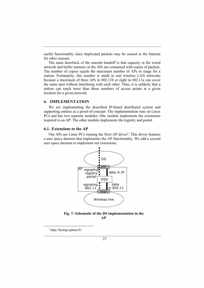
6. IMPLEMENTATION We are implementing the described IP-based distributed system and

supporting entities as a proof-of-concept. The implementation runs on Linux PCs and has two separate modules. One module implements the extensions required to an AP. The other module implements the registry and portal.

6.1. Extensions to the AP Our APs are Linux PCs running the Host AP driver1. This driver features

a user space daemon that implements the AP functionality. We add a second user space daemon to implement our extensions.

1 http://hostap.epitest.fi/

Wireless link

DS

wlan

eth

DSD

data in 802.11

signaling802.11

data in IPsignalingregistryportal

AP

Fig. 7: Schematic of the DS implementation in the

AP

38

Fig. 7 shows a schematic of the DS implementation in the AP. The AP has two interfaces: Ethernet to the DS and IEEE 802.11 WLAN to the wireless stations. The DS daemon (DSD) sends and receives messages from both. The DSD maintains two logical paths: one for signaling and another one for user data.

The DSD receives management signaling from the WLAN interface. Examples of theses management messages are association and hand off requests. The arrival of these messages to the DSD triggers the transmission of additional signaling messages through the Ethernet interface to the registry or portal, depending on the received messages as explained in the previous sections. In addition to receiving WLAN management messages, the DSD generates one type of IEEE 802.11 management message: beacons. These beacons are broadcast with the name of the WLANs that the AP is connected to.

The DSD participates in forwarding data frames as described in Section 4. It handles the encapsulation of data frames and makes the routing decisions inside the DS.

6.2. Registry and portal implementation We are implementing the registry and portal in a PC router running

Linux. Fig. 8 presents a diagram of the router including the registry and portal together with their signaling and data connections.

The registry is a user space program without special privileges that accepts connections in a TCP port. Its configuration information, such as

DS

Internet

eth

eth

Portal

data

signaling data in IP

Router

Registry

signaling

Fig. 8: Diagram of the registry and portal

implementation

39

name of the WLAN, is stored in local files. Dynamic configuration that is recorded during its operation, such as IP address of registered APs, is kept in memory.

The portal is a user space daemon. It requires special privileges to access directly to link layer drivers for data handling. The portal implements IP tunneling, handles packet encapsulation, downlink routing and n-casting during handoffs.

7. RELATED WORK To the best of our knowledge, this is the first paper that proposes an

implementation of the WLAN distribution system to facilitate large-scale deployments. El-Hoiydi surveyed the implementation options for the DS and its suitability for different scenarios [1]. However, the Ethernet-based DS is currently the only option available for APs with wired backbone.

Several large-scale deployments have been reported in recent years. They propose different solutions to deal with the shortcomings of the Ethernet-based DS. Hills described the WLAN network at Andrew University [2]. It uses a single Ethernet-backbone that spans several buildings in the campus. Their approach is to pay special attention to the interconnection of the switches so that there is enough capacity on every link and the spanning-tree protocol can handle the routing. They show that it is a valid solution for a campus-size network. However, it is not a general solution since WLAN operators do not always enjoy the freedom to deploy switches and connecting cables at will.

Escudero et al. presented a different architecture for a campus WLAN [3]. They split the wireless network into different areas. Inside an area, an Ethernet backbone connects the APs and link layer mobility is supported. When the stations move across areas, Mobile IP is used to maintain the connections. This approach works, but it adds the complexity of supporting Mobile IP in the wired networks and mobile stations.

Choi et al. presented NESPOT, the commercial WLAN-based Internet service of Korea Telecom [4]. It is a nation-wide WLAN with about 8700 hotspots in operation. Each hot spot can have one or more APs. Since the WLAN is designed and deployed by a nation wide ISP, it would be expected that roaming between hot spots would be supported. Instead link layer handoff is limited to the hotspots in which an Ethernet backbone is available. Building a single Ethernet backbone seemed unfeasible for this network size.

8. FUTURE WORK We have found a number of additional topics while designing our

distribution system that require further research.

40

• We have not analyzed the impact of using Network Address Translators (NAT) between APs and the registry or portal. The current design will not work in this case. One reason is that APs are identified by their IP address. Two APs behind the same NAT would appear with identical addresses to the portal. Another reason is that the portal and the other APs need to send encapsulated IP traffic to the APs behind the NAT. How to instruct the NAT to deal with these packets requires further studies.

• Fault detection of APs could be added to the DS. Currently, APs only contact the registry when they join the network. If they should fail later, the error is unnoticed. One possible solution is to add a heart beat protocol. It should be analyzed if the fault detection should be assigned to the registry or portal. In this line, a protocol supporting the disconnection of APs from the infrastructure should also be added.

• Performance monitoring follows fault detection. If added to the portal or registry, the operator can retrieve valuable information on the usage of their APs. This can be particularly useful in case of sharing APs.

• We did not deal with the issue of how to regulate the sharing of APs by different operators. Operators may want to have guarantees on their share of airtime. Some owners, such as residential users, may want to keep some airtime for their traffic. Sharing in these scenarios needs more analysis.

9. CONCLUSION Large-scale deployments of WLANs are exposing the limitations of the

WLAN architecture. We have addressed issues related to deployment, configuration and operation of WLANs whose APs are connected to different ISPs. We introduced two new entities, a portal and a registry, and redesigned the distribution system to work with IP packets. The new architecture supports self-configuration of APs, sharing APs between operators, connection of APs to different IP networks, transport of frames across the IP backbone, and station mobility at the link layer. An important feature of our design is that wireless stations do not require any modification to operate with the new architecture.

The smooth operation of large-scale WLANs is a large research problem. The work presented in this paper is a contribution towards this goal. Other aspects of the problem that need to be addressed include self-healing and protection against misbehaving users.

41

10. REFERENCES [1] Amre El-Hoiydi, "Implementation Options for the Distribution System

in the 802.11 Wireless LAN Infrastructure Network", in Proc. of IEEE ICC 2000, vol. 1, pp. 164-169, New Orleans, USA, June 2000.

[2] Alex Hills, "Large-Scale Wireless LAN Design", IEEE Communications Magazine, vol. 38, issue 11, pp. 98-104, November 2001.

[3] Alberto Escudero, Björn Pehrson, Enrico Pelletta, Jon-Olov Vatn, Pavel Wiatr, "Wireless access in the Flyinglinux.NET infrastructure: Mobile IPv4 integration in a IEEE 802.11b", in Proc. of 11th IEEE Workshop on Local and Metropolitan Area Networks LANMAN 2001, Boulder, Colorado, USA, March 2001.

[4] Youngkyu Choi, Jeongyeup Paek, Sunghyun Choi, Go Woon Lee, Jae Hwan Lee, Hanwook Jung, “Enhancement of a WLAN-Based Internet Service in Korea”, in Proc. of the 1st ACM international workshop on Wireless mobile applications and services on WLAN hotspots, San Diego, CA, USA, 2003.

[5] Héctor Velayos and Gunnar Karlsson, ”Techniques to Reduce IEEE 802.11b Handoff Time”, in Proc. of IEEE ICC 2004, Paris, France, June 2004.

[6] Ramachandran Ramjee, Thomas La Porta, Sandra Thuel, Kannan Varadhan, Shie-Yuan Wang, "HAWAII: a domain based approach for supporting mobility in wide-area wireless networks", in Proc. of Int'l Conference on Network Protocols, Toronto, Canada, October 1999.

[7] Charles E. Perkins and Kuang-Yeh Wang, “Optimized Smooth Handoffs in Mobile IP”, in Proc. of IEEE Symposium on Computers and Communications, pp.340 –346, July 1999.

[8] M. Zhang, B. Karp, S. Floyd, and L. Peterson, “RR-TCP: A Reordering-Robust TCP with DSACK”, ICSI Technical Report TR-02-006, Berkeley, CA, July 2002.

[9] M. Shin, A. Mishra and W. Arbaugh, “Improving the latency of 802.11 hand-offs using neighbor graphs”, in Proc. of ACM MobiSys 2004, June 2004.

[10] Anne H. Ren and Gerald Q. Maguire Jr., “An Adaptive Real-time IAPP Protocol for Supporting Multimedia Communications in Wireless LAN Systems”, in Proc. of International Conference on Computer Communications (ICCC´99), pp. 437 - 442, Tokyo, Japan, Sept. 1999.

[11] Hector Velayos, Victor Aleo and Gunnar Karlsson, “Load balancing in overlapping wireless LAN cells”, in Proc. of IEEE ICC 2004, Paris, France, June 2004.

43

PAPER B: LOAD BALANCING IN OVERLAPPING WIRELESS LAN

CELLS

45

Load balancing in overlapping wireless LAN cells

Hector Velayos, Victor Aleo and Gunnar Karlsson KTH Royal Institute of Technology

Stockholm, Sweden {hvelayos,victor,gk}@kth.se

Published in Proceedings of IEEE ICC 2004, Paris, France, June 2004

Abstract— We propose a load-balancing scheme for overlapping wireless

LAN cells. Agents running in each access point broadcast periodically the local load level via the Ethernet backbone and determine whether the access point is overloaded, balanced or under-loaded by comparing it with received reports. The load metric is the access point throughput. Overloaded access points force the handoff of some stations to balance the load. Only under-loaded access points accept roaming stations to minimize the number of handoffs. We show via experimental evaluation that our balancing scheme increases the total wireless network throughput and decreases the cell delay.

We would like to thank KTH Center for Wireless Systems and TeliaSonera for their support to this work

46

I. INTRODUCTION Wireless LANs are the predominant option for wireless broadband packet

access to the Internet. Their architecture, specified in the IEEE 802.11 standard, features a set of access points (APs) connected to a common Ethernet backbone. Each AP serves an area which radius depends on the bit rate and the type of environment. When the capacity of a single AP cannot accommodate the offered load in an area, several APs operating in different channels can be installed with overlapping coverage.

However, the capacity available does not increase with the number of APs in an area because stations typically select the AP that can be reached with the strongest signal to noise ratio. Since users tend to concentrate in some areas and the signal strength strongly depends on the distance, the AP closest to the users receives a higher number of stations [8][9]. Therefore, a load balancing mechanism must be added to the wireless LAN architecture.

We present in this paper our design of a load-balancing scheme for wireless LANs. It features a completely distributed architecture based on agents running at each AP. These agents send and receive load information via the wired backbone and select the stations that must hand off to balance the load. The main contribution of our design is the increase in total throughput and the decrease in cell delay achieved by uniformly distributing the load among overlapping APs. Additionally, our design can easily be deployed in an existing network because it works with standard wireless LAN stations and does not require any central server.

The rest of the paper is organized as follows. The related work is reviewed in Section II. The architecture of our load balancing system is presented in Section III, and its functional model is described in Section IV. Section V contains our experimental evaluation. Finally, we draw our conclusions in Section VI.

II. RELATED WORK The IEEE standard 802.11 specifies the architecture and protocols for

wireless LANs. For instance, it describes the operation modes, the medium access protocol and the physical interface characteristics. Several supplements to the standard extend its features. Examples of such supplements are the IEEE 802.11b and IEEE 802.11a, which add higher-speed physical layers in the 2.4 GHz and 5 GHz bands respectively. New supplements are expected to target particular problems. For instance, the IEEE 802.11e supplement will enhance the current 802.11 MAC to include quality of service. However, there is no standardization work to add load balancing in wireless LANs.

47

The commercial deployment of wireless LANs is demanding load balancing to effectively increase the capacity per spot. Due to the lack of a standard, some vendors have introduced proprietary solutions [2][3]. In short, they suggest adding load information to the beacon frames such as the number of users in the cell. Stations should use this information in addition to the signal strength to select the access points. There are two drawbacks to this approach. First, lack of interoperability between different vendors. Second, the stations do not cooperate to balance the load across the network.

The only research paper on load balancing in wireless LANs known to the authors is [6]. In this paper, Balachandran et al. present a load-balancing scheme based in a centralized access server that collects the load level at each AP and decides to which AP each station associates. The access server maximizes overall network utilization, but it is a single-point of failure and a potential bottleneck. Our work achieves the same goal with a completely distributed architecture instead of a centralized server.

III. ARCHITECTURAL DESCRIPTION Load balancing schemes can be used in wireless LANs if at least two

access points (APs) serve each physical location. Therefore, we assume a wireless LAN similar to the one depicted in Fig. 1. Reliability is the main reason for such architecture, since the failure of an AP does not create an area without coverage. Capacity provision is another important reason. When the offered traffic in a spot exceeds the capacity of a single AP, additional APs can be installed to increase the available capacity. In any case, APs with overlapping coverage should operate in different channels to avoid mutual interference. We also assume that all APs belong to the same wireless LAN network and thus are connected to the same Ethernet backbone.

0 1 2 3

7 6 5 4

Ethernet backbone

Figure 1. WLAN architecture with overlapping coverage

48

We add load balancing to wireless LANs by introducing a Load Balancing Agent (LBA) in each AP. Each LBA periodically broadcasts the load level of its AP to the common backbone. Using the reports from other LBAs, each LBA assesses whether the load is balanced among neighboring APs. If it is not balanced, it determines its AP state with respect to load sharing. There are three possible states: overloaded, under-loaded or balanced. Under-loaded APs are willing to accept new stations either roaming from neighboring APs or entering the network. Balanced APs only accept new stations joining the network. Overloaded APs do not accept additional stations and force the handover of current stations to reduce its load level.

This completely distributed architecture meets our easy-deployment goal in two ways. First, there is no need to modify existing wireless LAN stations. Second, there is no need to add a central server that collects the load levels and decides the best distribution of stations.

The load metric is one of the key elements in a load balancing system. The number of calls per cell is used in wireless networks such as GSM. This is a suitable metric in such networks because each voice call generates the same amount of traffic. However, Bianchi and Tinnirello showed that a metric based on the amount of traffic improves load balancing in wireless packet networks such as wireless LANs because each station generates a variable amount of traffic [1]. Several traffic-based metrics were presented in [1] such as the packet loss and the gross load including the number of stations and the retransmission probability. The same authors presented the number of competing stations as metric in [4]. Although we agree that these metrics show nice features, we need a different one that can be computed from the AP since one of our goals is to avoid modifications to the stations.

We use the throughput per AP, including uplink and downlink traffic, in bytes per second as the load metric. This is an adequate metric for our scenario because it is based on the traffic level and the AP can compute it without assistance from the stations.

Another important element in a load balancing system is the function used to measure the balance of the system. Comparing the throughput at different APs is not feasible because the varying nature of the traffic generated by the stations will always make these values different. Instead, we use the balance index β firstly introduced in [5] and used in [6]. Let Bi be the throughput at AP i, then β is defined as

( )( )∑∑

Β

Β=

2

2

i

i

nβ , (1)

49

where n is the number of neighboring APs over which the load is being distributed. The balance index is 1 when all AP have the same throughput and tends to 1/n when the throughput is severely unbalanced. The target for the load-balancing algorithm is to maximize the balance index.

The balance index quantifies the balance among neighboring APs, but it is not used to determine the APs state among overloaded, under-loaded or balanced. For this matter, the load at each AP is compared with the average load L calculated as follows

n

Li∑Β

= (2)

The APs with load below L are declared under-loaded and thus can accommodate more traffic. The APs with load above L are divided into two groups: overloaded and balanced. Overloaded APs are those which load exceeds the average by δ, while balanced APs are those which load exceeds the average by less than δ. The rational behind the parameter δ is to force the transfer of load from the most overloaded APs to those with load below the average L. The APs that are slightly over the average should not receive more load. Fig. 2 shows an example with four APs. The gray area in the figure highlights the balanced area. AP2 is balanced, while AP3 is overloaded. AP3 should transfer some load to either AP1 or AP4.

The parameter δ reduces the number of load transfers, but it also permits some unbalance since only APs exceeding the average load by δ will transfer some load.

Another important aspect of a load-balancing scheme is the policy to select the station that will be transferred from an overloaded AP. The simplest

Access point1 2 3 4

Load level

L

L+δL

Ove

rload

edar

eaU

nder

-load

edar

eaBa

lanc

edar

ea

Figure 2. Access points’ state with respect to the average load

50

policy is random selection. But it tends to produce many transfer decisions until the load is balanced. Instead, we have created a new policy called the best candidate aimed at reducing the number of transferred stations. The best candidate policy selects the stations which throughput is closest to the difference between the average load and the load at the AP.

Finally, we have designed a mechanism to transfer a station from an overloaded AP to an under-loaded one. The signaling specified in the IEEE 802.11 standard does not support this operation. Instead, the standard specifies that the stations can choose any AP in range. Our transfer procedure is a two-step process. First, the overloaded AP terminates the association of the station that should hand off by sending the standardized signaling message called disassociation notification. Second, the station searches and re-associates with another AP. If the station tries to re-associate with an overloaded or balanced AP, they will reject the request. Only under-loaded APs will accept the station. The drawback of this mechanism is that the station may need to try several APs until an under-loaded one is found.

IV. FUNCTIONAL DESCRIPTION The finite state machine of the LBA is shown in Fig. 3. The load

balancing actions are cyclically executed every Load Balancing Cycle (LBC). The cycle always starts calculating the balance index and finishes broadcasting the current AP load to other APs via the Ethernet backbone. If

Calculate β

Calculate L

Compute AP state

IF balanced IF overloaded IF under-loaded

Allow new stations

Allow new or roaming

stations

Deny new or roaming

stations

Transfer station

Broadcast load level

Wait LBC

β<1no

yes

Select best candidate

Figure 3. Finite state machine for the load balancing agent

51

the load distribution is balanced (i.e. β=1), no additional actions are performed. If the network is not balanced, then the average load L is calculated and used to determine the state of the AP. Depending on the state, the access rules are updated as indicated in the figure. Finally, if the state was overloaded, extra actions are taken to reduce the load before closing the cycle with the broadcast of the load level.

Overloaded APs transfer only one station per cycle. The station is selected with the best candidate policy and transferred with the signaling indicated above. During the station’s handoff, the load in the whole network is lower because the roaming station cannot transmit. To prevent that other APs change their state during this temporary load reduction, the overloaded AP waits in the transfer step until the notification of the re-association is received via the backbone. In this way, other APs use for their calculation the load level at the overloaded AP before the station transfer. As soon as the station is associated again, the overloaded AP transmit is new load level. The drawback of this procedure is that the load-balancing cycle that includes a station transfer might be larger than the desired LBC.

V. EXPERIMENTAL EVALUATION We have implemented the LBA as a proof of concept. Additionally, we

have used our implementation to measure the increase in total throughput and the decrease in delay when the traffic is balanced. The LBA was implemented as a user space process in Linux. Details of the implementation are available in [7]. The experimental setup consisted of two access points implemented in Linux using the Host AP driver1. In addition to the driver, each AP was running our LBA to implement the balancing system. During the tests, we used MGEN2 to generate UDP traffic and Trace Plot Real-Time3 to analyze the delay and throughput.

Preliminary experiments were conducted to determine the two parameters of our LBA: δ and the Load Balancing Cycle. During our performance experiments, we set δ to 10% and the Load Balancing Cycle to the wireless LAN beacon interval, i.e. 100 ms. This means that the difference in load between APs must exceed 10% to trigger the load balancing and that the LBA broadcast the load level once per beacon period.

We report one experiment to illustrate the increase in throughput and decrease in packet delay when using our balancing system. More experiments analyzing the performance of the load balancing are shown in [7]. The

1 http://hostap.epitest.fi/ 2 http://manimac.itd.nrl.navy.mil/MGEN/ 3 http://proteantools.pf.itd.nrl.navy.mil/trpr.html

52

experimental setup contained two APs with overlapping coverage and two stations. Each station generated 2 Mbps of UDP traffic and both stations were connected to the same AP at the beginning of the experiment. We run the experiment twice, the first time without load balancing and the second enabling it. During the second execution, the LBA transferred one of the stations to the other AP to balance the load. Fig. 4 shows the packet delay of the transferred station while Fig. 5 plots the station’s throughput. Both figures include the cases with and without load balancing to facilitate the comparison.

Fig. 4 shows that the average packet delay was 450 ms without load balancing. It also shows that there are three different phases in the experiment run with load balancing. Until time 13.6 s, the station was sharing the AP and thus the average delay was the same as without load balancing. Between 13.6 s and 16.6 s, the LBA forced the handoff of the station to the other AP and the station’s traffic was temporarily interrupted. After 16.6 s, the transmission is resumed via the new AP. The first packets suffered a markedly high delay because they were waiting in the wireless card buffer during the handoff. After these packets were transmitted, the packet delay reduced progressively as the kernel buffer was been depleted. At time 21.3 s, packets generated by the station were no longer buffered so the packets delay reduced to 8 ms in average.

The unexpectedly high handover time is due to misbehavior of the station’s wireless LAN card. When it receives the disassociation notification from the AP, it disconnect from the wireless LAN instead of reassociate with the other AP of the same network. Despite this firmware bug, the experiments show that delay was reduced from 450 ms to 8 ms due to load balancing. It also indicates that the number of load transfers should be minimized because

Figure 4. Station’s packet delay with and without load balancing

53

each one generates a temporary traffic interruption. A study of the handoff process and how to reduce its duration is presented in [10].

Fig. 5 presents the station’s throughput during the same experiment. Without load balancing, the station achieves an average throughput slightly over 1.5 Mbps in average. With load balancing the station reaches the expected 2Mbps after the load transfer is completed. There are also three phases in this plot. Before the handover, the station’s throughput was 1.5 Mbps. During the handoff, the station’s transmission is interrupted. After the handoff, the station temporarily transmits over the expected 2 Mbps throughput due to the buffered data. Comparing the achieved throughput in steady state after the handoff, i.e. at 23 seconds, the plot shows that the station increases its throughput by 500 Mbps due to the load balancing. Since the other station behaved in a similar way, the total throughput increased from 3 Mbps to 4 Mbps.

VI. CONCLUSIONS We have presented a distributed load-balancing scheme for wireless

LANs. Agents running in each AP exchange load information to determine whether their corresponding AP is overloaded, balanced or under-loaded. Balanced APs only accept new stations, while under-loaded APs accept new or roaming stations. Overloaded APs do not accept more stations and force the hand off of associated stations until the load is balanced. Since the standardized signaling does not support this operation, we have designed a two-step process to transfer a station. Firstly, the overloaded AP disassociates the station and then only under-loaded APs accept it. We have shown in our experimental evaluation that our balancing scheme increases the total network throughput and decreases the cell delay.

Figure 5. Station's throughput with and without load balancing

54

REFERENCES [1] G. Bianchi, I. Tinnirello, “Improving Load Balancing mechanisms in

Wireless Packet Networks,” IEEE International Conference on Communications, April 2002.

[2] Cisco Systems Inc., Cisco Aironet Access Points, September 2003, http://www.cisco.com/global/AP/aironet/prod_ftr.shtml.

[3] Proxim Wireless Networks, Orinoco Access Point Family, http://www.proxim.com/learn/library/datasheets/AP-2000_A4.pdf.

[4] G. Bianchi, I. Tinnirello, “Kalman Filter Estimation of the Number of Competing Terminals in an IEEE 802.11 network,” IEEE INFOCOM 2003, April 2003.

[5] D. Chiu and R. Jain, “Analysis of the Increase and Decrease Algorithms for Congestion Avoidance in Computer Networks,” Journal of Computer Networks and ISDN, vol. 17, June 1989.

[6] A. Balachandran, P. Bahl, G. M. Voelker, “Hot-Spot Congestion Relief in Public-area Wireless Networks,” Proc. of 4th IEEE Workshop on Mobile Computing Systems and Applications, June 2002.

[7] Victor Aleo, “Load distribution in IEEE 802.11 cells”, Master of Science Thesis, KTH, Royal Institute of Technology, March 2003.

[8] A. Balachandran, G.M. Voelker, P. Bahl, and P.V. Rangan, “Characterizing User Behavior and Network Performance in a Public Wireless LAN”, ACM SIGMETRICS 2002, June 2002.

[9] D. Kotz and K. Essien, “Characterizing Usage of a Campus-wide Wireless Network”, Technical Report TR2002-423, Dartmouth College, March 2002.

[10] H. Velayos and G. Karlsson, “Techniques to reduce the IEEE 802.11b handoff time”, IEEE ICC 2004, June 2004.

55

PAPER C: TECHNIQUES TO REDUCE IEEE 802.11B HANDOFF TIME

57

Techniques to reduce the IEEE 802.11b handoff time

Hector Velayos and Gunnar Karlsson KTH, Royal Institute of Technology


Published in Proceedings of IEEE ICC 2004, Paris, France, June 2004

Abstract—We analyze the link-layer handoff process in wireless LANs based on the IEEE 802.11b standard and suggest how to reduce its duration. Firstly, we divide the process into three phases: detection, search and execution. Our performance measurements indicate that the detection and search phases are the main contributors to the handoff time. We show that the link-layer detection time can be reduced to three consecutive lost frames. We also show that the search time can be reduced at least by 20% using active scanning with the two timers that control its duration set to 1 ms and 10.24 ms. Several simulations illustrate the achieved reduction in handoff time.

58

I. INTRODUCTION Wireless LANs based on the IEEE 802.11b standard are the predominant

option for wireless access to the Internet. The performance of the cells permits the use of real time services, such as voice over IP, when admission control is added and the MAC scheduler is modified [1]. However, experimental measurements in our testbed, which are summarized in Table I and described later, indicate that current implementations of link-layer handoff do not meet the needs of real time traffic.

In this paper, we propose and evaluate via simulations techniques to minimize the IEEE 802.11b handoff time. We describe the handoff procedure and divide it into three phases. Our main contribution is a set of techniques to reduce the two longer phases, detection and search. The rest of the paper is organized as follows. Section II describes the handoff procedure. Section III presents our measurements of current handoff implementations. Sections IV, V and VI contain our proposals to reduce each of the handoff phases, including simulation results to assess the time reduction achieved. Finally, Section VII summarizes our findings.

II. HANDOFF PROCEDURE Link-layer handoff is the change of the access point (AP) to which a

station is connected. In the case of IEEE 802.11b wireless LANs, the handoff implies a set of actions (e.g. change of radio channel, exchange of signaling messages) that interrupt the transmission of data frames. The duration of this interruption is called handoff time. The handoff procedure aims to reduce this time as much as possible so that upper layers do not notice the handoff, except for a temporarily higher delay on the link. Loss of packets during handoff is avoided by buffering frames in the station and in the old AP. When data transmission is resumed, these frames must be transmitted via the new access point. In addition, the infrastructure connecting the APs, typically a set of Ethernet switches, must be notified of the new position of the station in order to route the frames properly. These two actions lead to different handoff time for uplink and downlink traffic, the latter always being longer. Several authors have proposed solutions to make the uplink and downlink handoff time equal based on an adequate design of the distribution system [2] and the cooperation of access points via their wired interfaces [3]. Since the design of the infrastructure connecting the APs is outside the scope of this paper, we assume that such solutions are in place and thus downlink and uplink handoff times are the same.

The signaling to perform the handoff is specified in the Medium Access Control (MAC) protocol of the IEEE 802.11 standard and is common to the IEEE 802.11a, IEEE 802.11b and IEEE 802.11g supplements. Therefore, in

59

general, our work on handoff optimization can apply to all of them. However, our measurements and simulations focus on IEEE 802.11b.

We propose to analyze the handoff process by splitting it into three sequential phases: detection, search and execution. The detection phase is the discovery of the need for the handoff. The search phase covers the acquisition of the information necessary for the handoff. Finally, the handoff is performed during the execution phase. The following sections detail the events that occur during each phase.

III. MEASUREMENTS OF HANDOFF TIME The duration of each handoff phase was measured in our testbed. It

consists of two co-located IEEE 802.11b access points belonging to the same wireless LAN and connected to an Ethernet switch. Thus, stations can perform link-layer handoffs between APs. Each access point is a PC equipped with a D-Link wireless LAN card running Linux and the Host AP driver [4]. During the experiments, other PCs with the same driver were monitoring the activity on the radio channels. For the monitoring PCs, we developed software that captured the frames on the corresponding channel and calculated the duration of each handoff phase. Four commercial IEEE 802.11b cards with different chipsets were selected to measure their handoff time as an average of 10 repetitions. Each station’s handoff was measured independently. During the tests, the only traffic in the cells was a flow of packets generated by the station with the characteristics of voice over IP.

We noted in preliminary measurements that commercial wireless LAN cards take advantage of the information provided by the physical layer and completely skip the detection phase. These cards start the search phase when the strength of the received radio signal degrades below a certain threshold. Since we were interested in measuring the performance of the handoff using link-layer detection (i.e. without support from the physical layer), the handoff was forced by abruptly switching off the radio transmitter of the AP to which the station was connected. This allows assessing the importance of using the signal strength in deciding to start the handoff. Handoff measurements using physical layer information have already been reported by Mishra et al. [5]. It can be expected that a wireless LAN card implements both physical and link-layer detection. The later would be preferred in some situations such as wireless LANs featuring admission control or load balancing. In these cases, stations can loose the right to continue transmitting via the current AP regardless of the received signal strength.

As indicated above, we define the handoff time as the time during which the traffic was interrupted. Thus, in our experiments we measure the handoff

60

time from the first non-acknowledged data frame until the transmission of the first frame via the new access point.

Our handoff measurements are presented in Table I. From them we can draw the following conclusions. First, different stations showed different performance, but none matched the delay requirements of real time applications during handoff. Second, detection is the longest phase in all cases, while execution could be neglected. And third, detection and search times widely vary among different models. This was expected since the IEEE 802.11 standard only specifies the mechanisms to implement the handoff, but their combination and duration are left unspecified. The purpose was to allow the manufacturers some freedom to balance between different tradeoffs such as fast reaction or low power consumption.

The length differences in detection and search could be explained by analyzing the frames captured during the handoffs. This type of analysis produced the following conclusions. The need for handoff is detected at the link-layer after several non-acknowledged frames. The number of allowed failed frames is the main factor in controlling the duration of the detection phase. It varies with each card model because when a frame is not acknowledged, the station cannot differentiate whether the reason was a collision, congestion in the cell or the access point being out of range. Different cards use different assumptions depending on their purpose. For instance, the D-Link 520 is designed for a desktop PC, thus it assumes that the AP is always in range and retransmits for a longer period than the Orinoco card designed for laptops. Nevertheless, it was common to all the cards to reduce the bit rate and use the RTS/CTS mechanism after failed frames to overcome possible radio fading or collisions in an overloaded cell. Surprisingly, none of the analyzed models used the lack of beacon reception to discover that the access point was not in range. Regarding the search phase, all cards performed active scanning based on broadcasting probes to locate APs. The duration’s variance is due to the different number of probe requests sent per channel and more significantly due to the time to wait for probe responses.

The most detailed handoff measurements previously reported are [5]. Our measurements are in line with that work but numerical comparison is difficult because different cards were used. Additionally, their definition of handoff time does not include the link-layer detection phase. In their experiments, stations voluntarily started the search phase when the signal from the AP became weaker than a threshold.

The main conclusion from our measurements is that detection and search phases are the main contributors to handoff time. Therefore, we analyzed them in the following sections and suggest how they can be reduced.

61

IV. REDUCING THE DETECTION PHASE The actions during the detection phase vary depending on which entity

initiated the handoff. When the handoff is network initiated, the detection phase consists of a single disassociation message sent by an access point to the station. However, the most common handoff is the one initiated by the station, in which stations have to detect the lack of radio connectivity based on weak received signal reported by the physical layer or failed frame transmissions. QoS-concerned stations implement the former method because the handoff is initiated before any frame is lost. This method assumes that the density of APs is high and therefore, there is a better AP in range as soon as the received signal gets weak. On the other hand, the latter method produces less handoff events because the handoff is not triggered by temporary radio fading or interferences, but only when transmission is actually interrupted.

Our study focuses on the optimization of detection based on failed frames, i.e. link-layer detection without physical layer information. The main difficulty is to determine the reason for the failure among collision, radio signal fading, or the station being out of range. We have observed in our measurements that stations firstly assume collision and retransmit several times using lower bit rates. If transmission remains unsuccessful, then radio fading is assumed and probe request are sent to check the link. Only after several unanswered requests, the station declares the out of range status and starts the search phase. Different cards showed different detection times depending on the number of failed frames allowed and the number of probes sent. As Table I indicates, this type of detection procedure tends to be long, so we suggest a different approach: stations must start the search phase as soon as collisions can be excluded as the reason for failure. If the actual reason was a temporary signal fading, the selected access point after the search would likely be the current one and the handoff will not be executed. This means that independently of the duration of the fading, the data flow will be interrupted for the duration of the search phase, which further motivates the reduction of that phase.

Therefore, a key factor in our detection algorithm is the number of collisions that a frame can suffer before it is transmitted. Let C be the random variable representing the number of collisions per successfully transmitted frame. Its cumulative distribution function (CDF) is given by

1

0

1)1()(obPr +

=

−=−=≤ ∑ kk

i

i pppkC (1)

where p is the probability, seen by the station, that its transmitted frame collides. This probability depends on the number of stations competing for the medium, and it can be calculated with the non-linear system reported by

62

Bianchi in [6] for saturated conditions (i.e. all stations always have a frame ready to transmit) that is the worst case for collisions. The CDF of the number of collisions per transmitted frame is plotted in Fig. 1. This figure shows that three consecutive collisions is a rare event, even in saturation. Therefore, our link-layer detection algorithm can be formulated as follows: if a frame and its two consecutive retransmissions fail, the station can discard collision as the cause of failure and start the search phase; there is no need to explicitly probe the link. In the same conditions we used during our measurements, this time would be around 3 ms, which is approximately 300 times shorter than the fastest measured detection phase. A drawback of this link-layer detection algorithm is that its duration increases with the cell load and the transmitted frame length.

A special situation happens when stations are not sending traffic at the time of handoff, but only receiving. In this case, stations must track the beacon reception to differentiate between the situation when the access point has no traffic addressed to them or the AP is out of range. Stations must start the search phase after three beacons are missing and no traffic to other stations was received. Stations should not react at the first missing beacon because beacons can also be lost due to collisions. This converts the beacon period into another key factor to reduce the detection time. The shorter the period is, the shorter the detection time would be. But as the beacon period is reduced, more capacity is used for sending beacons instead of data frames. We have added beacon transmission to the ns-21 IEEE 802.11 module to evaluate this trade-off. Fig. 2 shows the result of our simulations for a saturated IEEE 802.11b cell. 1 ns-2 is a network simulator developed at the Information Science Institute, USC.

(http://www.isi.edu/nsnam/ns/)

Figure 1. No. of collisions per transmitted frame in saturation

63

This result confirms the expected behavior and allows selecting an adequate beacon interval. Currently, commercial IEEE 802.11b access points are shipped with a default 100 ms beacon interval. This means that approximately 4% of the AP’s capacity is used for beacons and that detection time based on three missed beacons would be 300 ms. Fig. 2 indicates that increasing the used capacity only to 6% would reduce the beacon interval to 60 ms. This would reduce by 60% the detection time (i.e. to 180 ms). Further reductions of the beacon interval, and thus the detection time, are possible but at the cost of noticeably decreasing the AP’s capacity.

V. REDUCING THE SEARCH PHASE The search phase includes the set of actions performed by the station to

find the APs in range. Since APs can operate in any channel of the allowed set, the IEEE 802.11 standard mandates that all allowed channels must be scanned. The standard also specifies two methods to scan a channel, active and passive scanning. In passive scanning, stations listen to each channel for the beacon frames. The main inconvenience of this method is how to calculate the time to listen to each channel. This time must be longer than the beacon period, but the beacon period is unknown to the station until the first beacon is received. Another problem is its performance. Since the whole set of allowed channels must be scanned, stations need over a second to discover the access points in range with the default 100 ms beacon interval. There are 11 allowed channels in USA, thus it would take 1.1 seconds. In most of Europe, there are 13 channels, so it would take 1.3 seconds.

When faster scanning is needed, stations must perform active scanning. Active scanning means that stations will broadcast a probe-request frame on each channel and wait for the probe response generated by the access point.

Figure 2. AP’s capacity used for beacon transmission in a saturated cell

64

The time to wait for responses depends on the channel activity after the probe transmission. If the channel is idle during MinChannelTime, i.e. there is neither response nor any kind of traffic in the channel, the scanning is finished and the channel is declared empty. If there is any traffic during this time, the station must wait MaxChannelTime. MaxChannelTime should be large enough as to allow the AP to compete for the medium and send the probe response. Both MaxChannelTime and MinChannelTime are measured in Time Units (TU). The IEEE 802.11 standard defines a TU to be 1024 microseconds. Note that scanning stations might not be able to sense other stations communicating with the AP, but they will always receive the acknowledgments sent from the AP and thus they will wait MaxChannelTime for probe responses.

Despite that MinChannelTime and MaxChannelTime control the duration of the scanning, the IEEE standard does not specify their values. We indicate in the rest of this section how to calculate them to minimize the search phase. First, we calculate MinChannelTime that is the maximum time an access point would need to answer given that the access point and channel were idle. If we neglect propagation time and probe response generation time, the IEEE 802.11 medium access function establishes that the maximum response time is given by

)( aSlotTimeaCWminDIFSTimeMinChannel ×+= (2)

where DIFS is the Distributed InterFrame Space, aCWmin is the maximum number of slots in the minimum contention window, and aSlotTime is the length of a slot. These values are defined in the IEEE 802.11b standard and inserting them in (2), we obtain 670 µs. Since MinChannelTime must be expressed in Time Units, we can conclude that MinChannelTime should be one TU (i.e. 1024 µs).

The calculation of MaxChannelTime is more complicated. It is the maximum time to wait for a probe response when the channel is being used. This time is not constant since it depends on the cell load and the number of stations competing for the channel. In order to find an upper bound for MaxChannelTime, we have run simulations to measure the time to transmit the probe response. Fig. 3 presents the results of our simulations. The probe response time shown is the average over 10 transmissions for each load level with channel bit rate set to 2 Mbps, the maximum possible rate for the probe response in IEEE 802.11b.

65

Our simulations confirm that the transmission time of a probe response depends on the offered load and number of stations. In addition, they also show that MaxChannelTime is not bounded as long as the number of stations can increase. We suggest then to set a value for MaxChannelTime that would prevent overloaded access points to answer in time. Since 10 stations per cell seems to be an adequate number to achieve a good cell throughput [6], Fig. 3 indicates that 10 TU (10.24 ms) would be a reasonable choice for MaxChannelTime.

Now that we have determined MinChannelTime and MaxChannelTime and that both timers are shorter than feasible beacon intervals, it is clear that active scanning is faster than passive scanning. Thus, active scanning should be used to minimize channel-scanning time.

Finally, we have to calculate the total search time that includes the time to scan all available channels. The number of available channels varies with regions. For instance, there are 13 possible channels in most of the European countries, while there are 11 in USA. Considering that the time to scan a channel is different depending whether it is been used, the total search time s can be calculated as

eu eTuTs += (3)

where u is the number of used channels (i.e with traffic) and Tu is the time needed to scan a used channel. Respectively, e is the number of empty channels and Te is the time to scan an empty channel. We can now determine Tu and Te. When a channel is scanned, a probe request is broadcasted and then the station waits for the probe response. Since the probe request is sent to the broadcast address, its reception will not be acknowledged. Therefore, at least two consecutive probe requests must be sent to overcome a possible collision.

Figure 3. Probe response transmission time (ms)

66

Each probe request must follow the same channel access procedure as the data packets, thus they will experience the transmission delay. Let Td be the transmission delay, then we can calculate Tu and Te as follows:

lTime MinChanne 2 TTe lTime MaxChanne 2 T T

d

du+=+=

(4)

The total search time can be calculated with (3) and (4), as well as the transmission delay. It increases with the number of used channels because MaxChannelTime is larger than MinChannelTime. This is illustrated in Fig. 4, which shows the total search time versus number of used channels in range for different load conditions. To plot it, we obtained Td from our delay simulations reported in Fig. 5. In Fig. 4, we used Td for an offered load of 50% with 5 and 10 stations per cell. In addition, we included a no-load case that is comparable with our measurements conditions reported in Table I. This case shows that the search time can be reduced to 70 ms when handing over between two APs, which is 20% faster than the shortest search phase measured.

These values in the x-axis of Fig. 4 are particularly interesting: one channel used would be the case of a search phase started due to radio fading when there are no other access points in range; two channels used would be the case of a handoff between two access points, the current and the new; and three channels used is an interesting value since it is the maximum number of channels that can share the same physical location without mutual interference.

Two problems regarding the search time must be highlighted. First, all access points in a given location affect the handoff time of stations, even access points belonging to different wireless LANs, because

Figure 4. Total search time (ms)

67

MaxChannelTime will be spent scanning their channels. Second, in areas with a high density of access points, search time can increase over the limits of real time applications. Both problems could be addressed with a small modification to the standard: the active scanning should not scan all available channels in a region (e.g. Europe or USA), but a shorter list with the channels actually used in the wireless LAN to which the station is connected. This is feasible since most wireless LANs use a fixed subset of the available channels. The list could be distributed as an additional field in the beacons.

VI. REDUCING THE EXECUTION PHASE The last phase is the execution of the handoff. To perform the handoff, the

station sends a reassociation request to the new access point and the AP confirms the reassociation sending a response with a status value of “successful”. This execution is the shortest possible, but the typical execution is longer because the new access point needs to authenticate the station before the reassociation succeeds.

The IEEE 802.11 standard specifies two authentication algorithms: open system and shared key. The open system is the default and equals to a null authentication algorithm. It involves the exchange of two frames, while the shared key algorithm requires a four-step transaction. Our measurements show that the execution phase using open system authentication is slightly over 1 ms for an empty cell, thus reducing the execution phase will not significantly reduce the total handoff time. Nevertheless, there are more complicated authentication schemes under study that require contacting an external server. In these cases, the authentication must be made before the handoff execution [7].

Figure 5. Delay versus load

68

VII. CONCLUSIONS We have measured, analyzed and suggested how to reduce the link-layer

handoff time in IEEE 802.11b networks. The handoff process was split into three sequential phases: detection, search and execution. We studied the detection based on failed frames (link-layer detection) instead of weak signal because it produces less handoff events. We have shown that the link-layer detection phase can be reduced to three consecutive non-acknowledged frames when stations are transmitting. In the same conditions we used during our measurements, this time would be around 3 ms, which is approximately 300 times shorter than the fastest measured detection phase. When stations are only receiving, we identified the beacon interval as the key factor in reducing detection time. Our simulations suggest 60 ms as an adequate beacon interval. We have also shown that using active scanning with its timers MinChannelTime and MaxChannelTime set to 1 ms and 10.24 ms respectively can reduce the search phase by 20% compared to the shortest measured one. Finally, the execution phase can be reduced with pre-authentication, but our measurements indicate that it is a very short phase and its reduction will not significantly decrease the total handoff time when using the current authentication methods.

REFERENCES [1] M. Barry, A. T. Campbell, A. Veres, "Distributed control algorithms for

service differentiation in wireless packet networks", Proc. IEEE INFOCOM 2001, Anchorage, Alaska.

[2] Amre El-Hoiydi, “Implementation options for the distribution system in the 802.11 Wireless LAN Infrastructure Network”, Proc. IEEE ICC 2000, vol. 1, pages 164-169, New Orleans, USA, June 2000.

[3] Anne H. Ren, Gerald Q. Maguire Jr., “An adaptive real-time IAPP protocol for supporting multimedia communications in wireless LAN systems”, Int. Conf. on Computer Communications, Japan, Sept. 1999.

[4] Host AP driver, http://hostap.epitest.fi/, last visit March 2004. [5] Arunesh Mishra, Minho Shin, Willian Arbaugh, “An empirical analysis

of the IEEE 802.11 MAC layer handoff process”, University of Maryland Technical Report, UMIACS-TR-2002-75, 2002.

[6] Giuseppe Bianchi, “Performance analysis of the IEEE 802.11 distributed coordination function”, IEEE Journal on Selected Areas in Communication, 18(3): 535 - 547, March 2000.

[7] Sangheon Pack, Yanghee Choi, “Pre-authenticated fast handoff in a public wireless LAN based on IEEE 802.1x Model”, IFIP TC6 Personal Wireless Communications 2002, Singapore, October 2002.

69

PAPER D: DISTRIBUTED ADMISSION CONTROL FOR WIRELESS LANS

71

Distributed admission control for WLANs

Hector Velayos, Ignacio Más and Gunnar Karlsson KTH, Royal Institute of Technology

16440 Kista, Sweden {hvelayos,nacho,gk}@kth.se

KTH Technical report TRITA-S3-LCN-0502

ISSN 1653-0837 ISRN KTH/S3/LCN/--05/02--SE

Abstract—This paper presents a distributed admission control for IEEE

802.11 wireless LANs that limits the packet losses due to congestion in a cell. This novel scheme requires no modification to the current distributed coordination function, and offers an upper bound for the average packet loss probability that flows will suffer in the wireless LAN cell. We show via extensive simulations that the admission control maintains the loss probability below the given threshold regardless of the offered load or number of stations. Our simulations also analyze the main drawback of this scheme: a reduction in the link utilization. The admission control offers soft QoS guarantees to multimedia flows without the need of complicated scheduling or polling mechanisms in IEEE 802.11.

This work has been partly supported by the European Union under the E-Next Project FP6-506869.

72

1. Introduction Wireless LANs based on the IEEE 802.11 standard suit are the

predominant choice for high-speed wireless access to the Internet. The IEEE 802.11 medium access control protocol was designed as an asynchronous best-effort service, and as such it does not offer capabilities to support quality of service (QoS) guarantees for real-time transmissions. As the interest in supporting multimedia services in WLAN is steadily increasing, the need to provide QoS guarantees equivalent to those in the wired network has to be addressed.

Two access schemes were specified in the IEEE 802.11 standard [10]. The point coordination function (PCF) was designed for contention free access. The PCF is a centralized scheme, in which the access point grants transmission permission to the stations that request it. It has never been commercially available, but it has originated some recent work on different polling schemes [1][2], or call admission control mechanisms [3]. Nevertheless, the dominant access scheme is the distributed coordination function (DCF), which features contention access whereby offering greater flexibility compared to the PCF. In favor of the DCF, previous work has shown that the PCF mode can have poor performance both alone and in cooperation with the DCF [4]. The main issue with DCF is the lack of QoS support. Current standardization work addresses how to modify the DCF to support priority schemes [11][12] suitable for multimedia transmissions [5]. The general approach has been to use some kind of priority scheduling under which the delay sensitive traffic can have priority access to the channel. All these approaches require modifications in the MAC protocol to implement the queue management.

We propose a distributed admission control for the standard DCF that offers QoS guarantees for the average packet loss due to congestion, and average transmission delay. Our proposal builds on the observation that the deployment of QoS mechanisms requires incremental steps and little changes in the hardware architecture and standardized protocols. In this sense, we want to provide a QoS scheme that uses the standard DCF mode and requires no modification in the MAC. The admission control works by performing a short, non-disturbing probing, which estimates what would be the average MAC service time after the new flow enters the cell. This average service time is then compared to an admission threshold, which is established to maintain the average packet loss rate below a configurable limit. The threshold is dynamically calculated at the access point and broadcasted in the beacons since it depends on the number of stations in the

73

cell and the load generated by those stations. The new flow is admitted if its MAC service time during the probing is below the threshold. Our admission control offers a trade-off between cell utilization and packet loss due to congestion. Congestion can be avoided by setting a low threshold for the MAC service time. In this case, multimedia flows can benefit from a bounded packet loss rate and can obtain an expected service time from the probing phase. This estimation facilitates buffer dimensioning for the mobile stations. Our scheme can be used alone or as a complement to the proposed priority scheduling to prevent congestion in the cell. In any case, our approach assumes a stable radio channel and thus we do not consider effects like fading or multi-path propagation, which could increase the losses.

Flow admission control has been advocated as a means to reduce overload situations and instabilities in network traffic, where network efficiency in overload can be improved by performing proactive admission control instead or relying on users impatience [6]. A clear phase change in the performance occurs when offered load in any network link exceeds its capacity. When the completion rate decreases, due to increased loss and increased offered traffic due to retransmissions, the effective throughput tends to zero. By limiting the number of flows in the system, the completion rate can be kept high, effectively clearing up bandwidth for new flows to enter. Furthermore, human perception favors consistency. The network should hence allow all kinds of sessions to complete when started without noticeable changes in quality that would annoy the user or might render the sessions useless. It is for example more acceptable to postpone a web surfing session that cannot be carried out reliably than to allow it to start with high uncertainty about the chances of completing it. Moreover, the proposed admission control scheme can be used as a means to enable an end–to–end admission control for a whole Internet path based on probe loss [7], or it can be used as a method to evaluate which cell would be more desirable in a load balancing scheme [8].

The rest of the paper is organized as follows. Section 2 presents the MAC service time in WLANs. Section 3 describes the probing procedure. Section 4 shows our simulation results. Section 0 contains the future work. Finally, Section 6 summarizes the main findings.

2. The MAC service time The delay of a packet crossing a wireless LAN cell can be split into three

parts: the delay at the medium access control (MAC), the transmission delay and the propagation delay. The propagation delay can be neglected due to the small size of the cells. The transmission delay can be easily determined

74

from the packet size and the bit rate used. The MAC delay is the most difficult to calculate because it depends on the traffic sent by the other stations in the cell. We divide the MAC delay into two parts: the service time and the queuing time. The former is the time to gain access to the shared channel for the transmission of the packet following the rules specified in the IEEE 802.11 standard. The latter is the time spent in the queue waiting for earlier packets to be transmitted.

Our admission control is related to packets’ delay, so we analyze in this section the service time for the IEEE 802.11 MAC protocol. We identify the number of stations competing for the channel as an important factor that affects the service time. We show via simulations that the service time may vary several orders of magnitude between consecutive packets sent from the same station. We also determine the average MAC service time and its standard deviation for different cell loads and numbers of stations.

2.1. Channel access procedure

The channel access procedure is defined in the IEEE 802.11 standard [10] and is common to all supplements such as IEEE 802.11a and IEEE 802.11b. As justified in the introduction, we focus our work on the DCF, one of the two channel access functions described in the standard. The DCF is a distributed access scheme in which all stations, including the access point, execute the same procedure to compete for the channel. The station that gains the channel transmits a single packet and enters the competition again if it has more packets to transmit.

The competition for the channel in the DCF works as follows. All stations with a packet ready to transmit choose a random number between 0 and 31. This number, called the congestion window, is the number of time slots that the station must sense the channel to be idle before it can start transmitting. The length of a slot depends on the physical layer (e.g. a slot is 20µs in IEEE 802.11b and 9µs in IEEE 802.11a). Since the different stations will likely choose different random numbers, this scheme is often collision free. However, two stations may choose the same congestion windows and a collision would occur. The chances of this event increase with the number of stations, but it is a rare and hardly impacts the overall performance [9]. When it occurs, it is solved via retransmission at the MAC layer.

There are some rules for decrementing slots from the congestion window. First, the station must sense the channel idle during a complete slot. If a transmission starts during the slot, the whole slot is considered used. Second, a packet transmission includes some periods in which the channel is idle. No slots can be discounted during these periods. For instance, the

75

channel is idle during some microseconds between the data packet transmission and its acknowledgment. This time cannot be used to discount slots. Third, after a transmission of a frame is completed (including the acknowledgment) the station must sense the channel to be idle during an interval called Distributed Inter-Frame Space (DIFS) before decrementing new slots.

When a station reaches zero, it can transmit. In the basic access, the station transmits a single packet and waits for the acknowledgment to confirm its reception. If the optional Request To Send, Clear To Send (RTS/CTS) signaling is enabled, the station transmits a RTS frame to notify the rest of stations that it is about to start a transmission. The access point confirms the RTS reception sending a CTS frame. When the CTS frame reaches the station, it transmits the data frame and waits for the acknowledgement. In any case, if the acknowledgment is not received, the station retransmits the frame. On each retransmission, the same procedure is used with the exception that the interval from which to choose the congestion window is doubled. A packet can be retransmitted a maximum of 7 times, although the congestion window interval is doubled only the first 5 times. The side effect of doubling the congestion window interval is that stations retransmitting gain the channel less often than stations transmitting a packet for the first time. This is called the capture effect and affects the fairness of the access scheme when some stations often need to retransmit due to poor radio conditions. Nevertheless, it may increase the link throughput because stations with good channel conditions tend to transmit more often.

This access scheme is fair in the sense that each station receives the same number of transmission opportunities in the long term. If all stations use similar bit rates and experiment comparable number of retransmissions, then they achieve the same throughput. However, each station’s throughput decreases in equal proportion if the offered traffic exceeds the cell’s capacity. Our admission control addresses this problem by limiting the number of flows that stations can generate so that congestion is avoided.

2.2. Analysis

The mathematical analysis of the IEEE 802.11 MAC service time based in the Markov model proposed for throughput analysis produces average values for saturation conditions (i.e. all stations ready to transmit) [9]. Since we are interested in the service time of each packet in a flow for bursty traffic sources, we simulate the access link to get these results. We have used

76

the Network Simulator 21 for our simulations. The only addition was a monitoring agent to measure the MAC service time. A single cell is simulated where each station has the same contribution to the cell load, which ranges from 5% up to 100%, increasing in steps of 5%. The number of stations in the cell n is a parameter in our simulations. The bursty traffic of each station is generated according to an exponential on-off traffic source. The average on-time ton is 20 ms and the average off-time toff is 35 ms. If

the desired cell load is l, the rate of each station during the on period is calculated as follows:

.)(nl

ttt

rateon

offon +=

During the simulations, n-1 stations generate traffic and we measure the service time of the n-th station. The results reported in the next section correspond to the measurement of 50 packets per run. We repeat the simulation with different random seeds 30 times to calculate the average service time. All simulations use a fixed packet size equivalent to the default TCP segment size (approximately 500 bytes), and there are no retransmissions due to poor radio conditions. The following figures present two types of results for the MAC service time. First, we show the service time per packet for different load levels. Then we show the average service time and its standard deviation for different load levels using the number of stations as a parameter.

Fig. 1 shows the MAC service time per packet in a cell with 10 stations for three load levels. Low load corresponds to an offered load equivalent to 15% of the channel capacity, high load to 60% of the channel capacity, and overload to 90% of the channel capacity. The cell operates without losses only at low and high loads. In overload, the traffic in excess is dropped. The subplots in Fig. 1 show the service time per packet and the running average. The running average is the average of the service time including all packets previously transmitted and is updated after each packet transmission.

We can draw these conclusions from Fig. 1. There are always packets whose service time is below one ms regardless of the offered load. For these packets, the station can decrement all slots in the congestion window without interruptions due to transmission. This case is always possible, although its probability decreases when the load increases. This is confirmed comparing the subplots in Fig. 1. The number of occasions in which the service time is below 1ms is much higher in the first subplot than in the last one.

1http://www.isi.edu/nsnam/ns/

77

Fig. 1: IEEE 802.11 MAC service time per packet for different cell load.

78

The maximum service time for a packet depends on the cell load. The higher the load, the higher the service time could be. The peaks shown in the service time correspond to cases in which the congestion window decrement is interrupted by transmissions from other stations. The probability of this event grows with the load. The difference between peaks in the same subplot is related to how many packets interrupted the slot discount.

There is no correlation between the service times of two consecutive packets. This was expected from the access channel procedure since each packet is transmitted independently of any other using the same rules. Fig. 1 confirms this assumption.

Despite the differences in service time between packets, the running average stabilizes quickly; around 20 packets are enough to get an accurate value. Nevertheless, the average is a poor indicator of the service time for individual packets as shown in the subplots.

Fig. 2 shows the average service time for different load levels and the standard deviation for the average service time. In both figures, we use the number of stations as a parameter. Both figures indicate that the number of stations starts to be important only when the offered load is above 60%.

If the offered load is below 60%, the average MAC service time seems to be small. But the standard deviation is of the same order of magnitude as the average. This indicates that the service time of the packets is widely spread around the average. Some packets may experience service times in the order of tens of milliseconds. An example of such packets is visible in the middle subplot of Fig. 1. Therefore, the MAC service time cannot be neglected for some applications with a tight end-to-end delay requirement for every packet. A typical application of this type is voice over IP that requires a maximum of 150 ms end-to-end delay for every packet. A MAC service time of around 20 ms for some of the packets may be excessive.

3. The probing scheme The purpose of our admission control is to determine whether a new

flow can be accepted to the cell without compromising the QoS of the existing flows. The decision is taken at the station originating the new flow since we aim at a distributed scheme. One possibility is that the station with a flow tries to estimate the cell’s load by listening to the channel. Unfortunately, the station may not receive all transmissions in the cell. Therefore, this method would likely result in an under estimation of the cell’s load. Another possibility is that the station starts the new flow and monitors its packet losses. If the losses exceed a certain limit, the flow should be stopped. Although this scheme would work, existing flows in the

79

cell are likely to suffer similar looses since the MAC protocol gives the same number of transmission opportunities to each station. The new flow would be blocked too late. Instead, we propose that the station with the new flow performs active measurements to determine if the new flow can be accommodated. The main goal of our probing scheme is to perform these measurements in a way that gives enough information to perform an accurate admission decision, but does not produce significant disturbances in the ongoing traffic.

Our admission decision is based on a comparison with the average MAC

Fig. 2: Average and standard deviation of the IEEE

802.11 MAC service time as a function of the cell load

80

service time that the cell experiences for a particular utilization. The maximum utilization we permit in the cell is given by the target packet-loss probability that we want to enforce. The only information the station requires to perform the admission decision is the admission threshold. We suggest that the access point includes this value together with the other cell information that is periodically broadcast in the beacon. The access point determines the threshold from the number of stations in the cell and the desired upper bound for the average packet loss probability. The number of stations is always available at the access point because it grants connection authorizations, and the bound for the loss probability must be provided as a configuration parameter. We describe in the subsection below the procedure to compute the threshold and give the threshold values for a couple of cases.

The probing procedure works as follows: When a station wants to start transmitting a new flow, it sends 50 probe packets at the flow’s peak rate with a probe packet size of 500 bytes. Ideally, the probe size should be equal to the average packet size of the flow, but this information is unknown at the time of the probing. Instead, we use a fixed size that is close to the average packet size on the Internet backbones2. The time required to complete the probing depends on the flow’s peak rate. For instance, a flow with 1 Mbps of peak rate would complete the probing in about 200 ms.

The train of probe packets interacts with the ongoing flows, thus experiencing a service time similar to the service time of the new flow if it would be accepted. The station measures the service time of each probe packet and determines the mean service time of the probes. If RTS/CTS is enabled, the RTS service time should be measured instead. The obtained mean is compared to the admission threshold received in the last beacon. If the mean is smaller than the admission threshold, the new flow is accepted. Otherwise, the flow is rejected and has to back off for a certain time before performing a new attempt to enter the cell.

The effect of the probing phase on the ongoing sessions depends on the load in the cell and the number of stations. The evaluation of our admission control, presented in Section 4, shows that the probing does not significantly affect ongoing sessions, and yet permits making correct admission decisions.

3.1. Finding the admission threshold

The admission threshold is the mean service time for which the mean packet-loss probability in the cell is equal to the target. The admission threshold is calculated in two steps. In the first step, we determine which is

2Sprint IP monitoring project, http:\\ipmon.sprint.com

81

the offered load that corresponds to the target loss probability. From our simulations, we have obtained the relation between mean packet-loss probability in the cell and offered load. This relation is shown in Fig. 4 for 4 and 10 stations. Each point of the plot for an offered load was obtained by averaging the mean packet-loss probability for 30 simulation runs with different random seeds. The data in Fig. 4 shows that there is no packet loss when the offered load is lower than 50%, and that there is an offered load value after which the packet-loss probability increases roughly linearly. This value depends on the number of stations in the cell. The higher the number of stations, the lower the value because congestion is reached earlier. The slope at which the loss probability increases also depends on the number of stations. The smaller the number of stations, the higher the slope because there is less buffer space in a smaller group of stations. The linear behavior of the loss probability function permits us to determine the offered load corresponding to the target loss probability. For example, if we select a target loss probability of 2.5%, we obtain from Fig. 4 that the maximum offered load in the cell should be approximately 72% and 79% of the link capacity for 4 and 10 stations, correspondingly.

In the second step to calculate the admission threshold, we determine a suitable service time that indicates that the offered load is equivalent or slightly lower than the value obtained in the previous step. Fig. 2 shows the mean service time as a function of the offered load. The mean service time is

Fig. 3: Admission threshold as a function of the

number of stations in the cell for 0.5% and 2.5% packet loss probability.

82

not appropriate to determine the offered load due to its high standard deviation. We rather choose the minimum mean obtained during the 30 independent simulation runs that produced the mean service time shown in Fig. 2. This conservative option produces a lower admission threshold. We show in the evaluation below that this results in higher unnecessary blocking, but virtually eliminates the wrong admissions.

The two-steps procedure allows calculating the admission threshold for the desired target loss probability as a function of the number of stations. An example of the result is show in Fig. 3 for two target loss probabilities: 0.5% and 2.5%. For instance, the admission threshold would be 4.25 ms for the target packet loss probability of 2.5% if there were six stations in the cell.

Fig. 3 shows two profiles for the admission threshold as a function of the number of stations. The threshold for 2.5% packet loss increases with the number of stations, while the number of stations does not affect the threshold for 0.5%. The first threshold corresponds to a loss probability high enough to permit a light congestion; therefore, some packets wait until the transmission of packets from other stations is completed. It is natural that the maximum service time (i.e. the admissible threshold) increases with the number of stations. Ten stations have more buffer space than 4 stations to store packets while the first in the queue is transmitted. The second threshold completely prevents the congestion so the maximum service time is independent of the number of stations. The offered load is low enough so that most of the packets are transmitted as soon as they reach the link layer. They do not have to wait for transmissions from other stations to complete.

4. Evaluation We have implemented our admission control in ns-2 to evaluate its

behavior and performance. There were three goals for our evaluation: First, we wanted to show that our admission control effectively keeps the packet-loss probability below the target; second, we desired to compare the achieved link utilization with and without admission control; and third, we wanted to analyze the correctness of the decisions taken by the admission control.

Our evaluation is based on simulations. We study the different aspects of the admission control as a function of the offered load. The offered load is expressed as a percentage of the link capacity and varies from 5% to 100% in steps of 5%. Each offered load value is simulated 30 times with different random seeds. The results in the plot are the mean of the 30 repetitions. The number of station is used as parameter. Two values are shown: four and ten stations. In all simulations, we have used the same type of bursty sources

83

described in the analysis of the MAC service time in Section 2. The target packet-loss probability of 2.5% is also common to all simulations. Therefore, the admission thresholds given in Fig. 3 are used when admission control is enabled

Fig. 4 depicts the mean packet loss probability in the cell for different offered loads, with and without admission control, for 4 and 10 stations. The admission control is set to keep the packet-loss probability below 2.5%. The figure clearly shows that the packet loss probability grows almost linearly from an offered load of around 60% of the link capacity when there is no admission control. When our admission control is enabled, the packet-loss probability remains well below our target packet-loss probability of 2.5%, regarless of the offered load or number of stations.

Fig. 5 shows the link utilization with and without admission control for different offered loads. The utilization for 4 stations without admission control was omitted for clarity since it virtually overlaps with the utilization for 10 stations without admission control. It can be seen that there is a slight decrease in utilization at high offered loads when the admission control is enabled. This is due to the fact that some sessions are blocked to avoid the losses due to congestion. Lower link utilization is the main penalty of our admission control.

Another important observation is the effect that the number of stations has on the achieved utilization. The lower the number of stations, the lower the link utilization. This effect is consequence of our simulated scenario in

Fig. 4: Packet loss probability for 4 and 10 stations as

a function of the offered load with and without admission control.

84

which each station generates the same amount of traffic. This means that blocking one out of four flows represents a higher reduction in offered traffic than blocking one out of 10 flows. This effect is then more related to the size of the sessions being setup than to the number of stations in the cell.

Finally, we show the performance of the admission control in Fig. 6 by classifying the admission decisions into three subsets: correct decisions, wrong decisions and unnecessary blocking. Wrong decisions are those in which the admission control fails to bound the packet loss ratio in the cell, i.e. after admitting a new flow the cell experiences a packet loss probability above 2.5%. Unnecessary blocking occurs whenever a new flow is not admitted, although the loss probability in the cell would not have grown over our target value had it been admitted. As a design decision, we wanted to minimize the number of wrong decisions, risking to increase the unnecessary blocking and thereby to decrease the utilization. The figure shows that our admission threshold meets our design choice. There are a negligible number of wrong decisions while the unnecessary blocking is only high near the theoretical limit of the load that should be accepted. Around 60% of offered load new flows are rejected while some of them could have been accepted and still meet our packet loss criteria. However, once the offered load increases over 80% most of the flows are correctly rejected. A less restrictive admission control would achieve higher utilization, but would have risked admitting sessions that could suffer a higher packet loss probability than our target.

Fig. 5: IEEE 802.11 cell utilization as a function of

the offered load with and without admission control.

85

5. Future work There are a number of related problems to our admission control for the

DCF that need furher study. • We have fixed the probing length to 50 packets since it produced mean

service time measurements accurate enough for our purposes. A deeper analysis of the required probing length may result in a reduction of the probing phase.

• Our admission control requires the participation of the access point. The admission threshold is dynamically calculated at the access point as a function of the number of connected stations and the target packet-loss probability. A different way to determine the admission threshold must be investigated so that our admission control can also be used in ad-hoc networks.

• The selection of our admission threshold may be considered too restrictive. Most flows are blocked as soon as the offered load approaches the desired limit. Alternative selection strategies could be researched and compared to our choice.

• Our admission control is flow based. If a station sends several flows, the admission control is applied to each one independently. Our simulations focused in the case with one flow per station. Further simulations should validate that the admission controls also works for

Fig. 6: Admission control performance as percentage of correct, wrong and unnecessary blocking decisions

as a function of the cell’s load

86

the case with several flows per station. • We have designed and validated our admission threshold with a single

traffic pattern: exponential on/off. Additional simulations are needed to validate that our admission controls works fine regardless of the traffic pattern.

6. Conclusions In this paper, we have presented a distributed admission control for the

DCF of IEEE 802.11 wireless LANs that guarantees an upper bound on the mean packet-loss probability due to congestion. The admission decision is based on comparing the measured service time of a short, non-disturbing probing with a given admission threshold. We have described how to calculate the threshold as a function of the number of stations and target loss probability. The probing provides an estimate of the expected service time, which can be important for multimedia flows. We have evaluated the performance of our admission function showing the percentage of correct and wrong decisions, as well as the amount of unnecessary blocking. The evaluation shows that 50 packets are enough to perform an accurate decision that effectively limits the mean loss probability in the cell.

As a preliminary step, we have analyzed the IEEE 802.11 MAC service time per packet and on average. We have found that the service time for a packet cannot be easily predicted. It can be below one ms for any offered load or reach tens of milliseconds for high loads. However, the mean service time quickly reaches a stable value that can be estimated after transmitting a few packets. We have taken advantage of this finding in the design of our admission control.

The main drawback of the proposed admission control is a reduction in the link utilization. We have shown that this reduction depends on the number of nodes in the cell and, of course, on the size of the sessions being set up. Nevertheless, we believe that the levels of utilization achieved are acceptable.

References [1] J. Y. Yeh and C. Chen, “Support of multimedia services with the IEEE

802-11 MAC protocol,” in Proc. of IEEE ICC 2002, pp. 600–604, 2002. [2] C. Coutras, N. Gupta, and N. Shroff, “Scheduling of real-time traffic in

IEEE 802.11 wireless LANs,” Wireless Networks, vol. 6, no. 6, pp. 457–466, 2000.

[3] M. Veeraraghavan, N. Cocker, and T. Moors, “Support of voice

87

services in IEEE 802.11 wireless LANs,” in Proc. of the 20th Infocom, (Anchorage, Alaska), pp. 488–497, IEEE, April 2001.

[4] A. Lindgren, A. Almquist, and O. Schelén, “Quality of service schemes for IEEE 802.11: A simulation study,” in Proc. of IWQoS 01, vol. 2092 of LNCS, (Karlsruhe, Germany), p. 281, Springer, Jun 2001.

[5] Y. Xiao, H. Li, and S. Choi, “Protection and guarantee for voice and video traffic in IEEE 802.11e wireless LANs,” in Proc. of the 23rd Infocom, (Hong Kong, China), IEEE, March 2004.

[6] J. W. Roberts, “A survey on statistical bandwidth sharing,” Computer Networks, vol. 45, pp. 319–332, March 2004.

[7] I. Más Ivars, V. Fodor, and G. Karlsson, “The performance of endpoint admission control based on packet loss,” in Proc. of QoFIS 2003, vol. 2856 of LNCS, (Stockholm, Sweden), Springer, October 2003.

[8] H. Velayos, V. Aleo, and G. Karlsson, “Load balancing in overlapping wireless lan cells,” in Proc. of IEEE ICC 2004, (Paris, France), June 2004.

[9] G. Bianchi, “Performance analysis of the IEEE 802.11 distributed coordination function,” IEEE Journal on Selected Areas in Communications, vol. 18, pp. 535–547, March 2000.

[10] LAN/MAN Standards Committee of the IEEE Computer Society, "IEEE Std 802.11-1999, Wireless Lan Medium Access Control And Physical Layer Specifications", USA, August 1999.

[11] IEEE 802.11 working group task e, "Draft supplement to standard 802.11-1999 wireless medium access control and physical layer specifications: medium access control enhancements for quality of service (QoS)", IEEE 802.11e/D2.0, November 2001.

[12] Y. Xiao, “IEEE 802.11e: QoS provisioning at the MAC layer”, IEEE Wireless Communications, vol. 11, issue 3, pp. 72-779, June 2004.

89

PAPER E: STATISTICAL ANALYSIS OF THE IEEE 802.11 MAC SERVICE

TIME

91

Statistical analysis of the IEEE 802.11 MAC service time

Hector Velayos and Gunnar Karlsson KTH, Royal Institute of Technology


To appear in Proceedings of the 19th International Teletraffic Congress,

Beijing, China, August 2005.

Abstract— We present a statistical analysis of the IEEE 802.11 MAC

service time. Our analysis complements the results from mathematical models, which focus on the mean delay. The location analysis shows that the service time’s distribution is skewed: the mean is always larger than the median, and the mode is always the smallest. A deeper analysis of the mean illustrates its dependence on the number of stations in the cell, the offered load, the packet size and the bit rate. The analysis of variability includes the coefficient of variation of the service time and its cumulative distribution function. The high variability found indicates that the 95-percentile of the service time may be a more meaningful measure than the mean. Finally, the analysis of correlation demonstrates that the service time of a packet is not predictable from the service time of previous packets.

Keywords—IEEE 802.11 MAC, service time, analysis. This work has been partly supported by the European Union under the E-Next Project FP6-506869

92

1. INTRODUCTION

Information about the expected delay in communication networks is vital for most applications. Interactive multimedia requires a limited end-to-end delay to reach acceptable quality levels. Streaming of multimedia contents uses delay measurements to compute the size of the play-out buffers for jitter compensation. Elastic flows such as web browsing relay on the ability of TCP to predict the end-to-end delay for triggering retransmissions. These examples explain the recent research interest in delay studies for different networking technologies. In particular, the delay in wireless LANs (WLANs) based on the IEEE 802.11 standards has received much attention lately, since it is the most popular option for high-speed, packet-based wireless access to the Internet.

The delay of a packet in a WLAN can be split into three parts: the delay at the medium access control (MAC), the transmission delay and the propagation delay. The propagation delay can be neglected due to the small size of the cells. The transmission delay can be easily calculated from the packet size and bit rate used. The MAC delay is the most difficult to determine because it depends on the traffic in the cell. We divide the MAC delay into two parts: service time, or time to gain access to the shared channel following the rules specified in the IEEE 802.11 standard, and the time spent in the queue waiting for earlier packets to be transmitted. We focus our study on service time, since queuing delay is the consequence of packet inter-arrival times being shorter than the service times.

The growing interest in quality of service has fueled the publication of models for the delay in the IEEE 802.11 MAC protocol. The analysis of MAC service time is a key part of these models. A common assumption for early models is that stations are always ready to transmit (saturation). There are several examples of such models. Chatzimisios et al. studied the packet delay in presence of transmission errors [1]. Their model is an evolution of Bianchi’s model based on Markov chains for throughput analysis in ideal channel conditions [2]. Tay and Chua suggested a different model based on stochastic analysis that provides throughput and packet delay [3]. Carvalho and Garcia presented another model for the MAC delay as a function of the channel state probabilities [4]. Unfortunately, these probabilities can only be

93

calculated under the assumption of saturation. All these models provide mean service time in saturation; they cannot be used for non-saturating loads. Nevertheless, their output values can be used as upper bounds for the service time. Banchs suggested an approximated expression for the distribution of the backoff delay (equivalent to the service time) in saturation [5]. His work permits a better understanding of the service time in saturation compared to previous models that only provided the mean.

The saturation condition was relaxed in two models recently published. Tickoo and Sikdar presented a queuing model for the average service time valid for non-saturating loads and arbitrary arrival patterns [6]. Their model determines the mean service time from average inter-arrival times for traffic sources. Li and Battiti suggested another model for non-saturation in which the mean service time can be derived from the probability that a station’s transmission queue is empty after the successful transmission of a packet [7]. None of these models provide information about service time for individual packets.

There are two limitations in existing models. First, they only provide the mean MAC service time; the variability of the packet delays is not modeled. Second, they assume that the number of stations in the cell is large enough so that the probability of packets colliding is constant and independent of the transmission time. However, measurements with real equipment are not a valid alternative to these models to obtain more information about the MAC delay. Packet timestamps in commercial WLAN cards are not accurate enough and include other delays not related to the MAC protocol operation.

In this paper, we present a statistical analysis of the IEEE 802.11 MAC service time based on simulations. Our analysis extends the mathematical models providing packet level information for small number of stations. Output from our analysis includes histograms, mean and variability, cumulative distribution functions, and autocorrelation plots. We show that the service time distribution is skewed and the variability increases with the load. Applications with strict requirements on delay per packet may consider the 95-percentile better than the mean as an indicator of the expected delay. We also show that there is no significant correlation between the service times experienced by the packets of a flow. Hence, the service time of future packets cannot be inferred from previously measured values.

The rest of the paper is organized as follows. Section 2 describes the

94

channel access procedure of the IEEE 802.11 MAC protocol. Section 3 details our methodology for the analysis. Section 4 presents the analysis of location in which the distribution of service time is analyzed; Section 5 contains the analysis of variability, and Section 6 provides the analysis of autocorrelation. Finally, Section 7 closes the paper by summarizing the main findings.

2. CHANNEL ACCESS PROCEDURE

The MAC service time is the time required by a station to access the channel in competition with the other stations within the cell. The channel access procedure is defined in the IEEE 802.11 standard and is common to all later supplements for higher rates (e.g. IEEE 802.11a and IEEE 802.11g). The standard describes two coordination functions for accessing the shared medium. The point coordination function (PCF) is a centralized access scheme in which the access point grants the channel to stations that request it. The PCF was never deployed commercially. Instead, the distributed coordination function (DCF) is used. We therefore restrict our study to the DCF access scheme, in which all stations, including the access point, execute the same access procedure to compete for the channel. The station that gains the channel transmits a single packet and enters the competition again when it has more packets to transmit.

The DCF access procedure can be summarized as follows. All stations with a packet ready to transmit choose a random number uniformly distributed between 0 and 31. This number, called the congestion window, is the number of time slots that a station must sense the channel to be idle before it can transmit. Since the different stations will likely choose different random numbers, this scheme is collision free in most of the cases. However, there is a possibility of collision if two stations choose the same number. The chances of this event increase with the number of stations, and when it occurs, it is solved via retransmission at the MAC layer.

When a station has decremented the number of slots to zero, it transmits a single packet and waits for the acknowledgement to confirm the reception. If the acknowledgment is not received, the transmission was unsuccessful and the station retransmits the frame. On each retransmission, the station doubles the size of the interval from which to select the congestion window. So, it will

95

wait longer on average before retransmitting. A packet can be retransmitted a maximum of 7 times, although the congestion windows is doubled only the first 5 times.

According to this access procedure, the service time depends on four factors: the number of stations, offered load, packet size, and bit rate. The first and second control how strong the competition is for the channel. The third and fourth factors affect how long a station captures the channel for transmission. High competition and long capture times tend to increase the service time.

A new coordination function called Extended DCF (EDCF) is being standardized by the IEEE work group 802.11e. It divides the channel time in cycles composed of contention and contention free periods. The contention free period aims at providing bandwidth and delay guarantees to stations, and works via reservations at the access points. The contention period operates under the DCF and therefore most conclusions of our study are useful for the EDCF.

3. ANALYSIS METHODOLOGY

We have used ns-21 to simulate the IEEE MAC 802.11 access link and analyze the service time. We only added a monitoring agent to measure the service time per packet. A single cell is simulated in which a set of stations transmit towards a destination node connected to the access point via a wired link of 100 Mbps. Packet losses during simulation are only due to collisions or buffer overflow; the cell operates with an ideal radio channel. Stations are uniformly distributed along a circumference of radius 20 meters with the access point in its center. Physical and MAC layer parameters are set according to the IEEE 802.11b standard.

During the simulations, a warm-up period of one minute precedes the measurement of the service time. The service time is measured for a single station during 10 seconds. Since the seed of the simulator’s random generator heavily influences this result, we repeat the measurement 20 times using different seeds. The results shown in the next sections are averages of the 20 runs.

1 http://www.isi.edu/nsnam/ns/

96

The four parameters affecting the service time were varied during simulations to study their influence on the results. The number of stations was 4, 7 or 10. The packet size was 40 bytes, 500 bytes or 1500 bytes. According to CAIDA2 reports, the packet size distribution on the Internet backbones peaks around these values. The bit rate varied between 2 Mbps, 11 Mbps and 54 Mbps, which is the highest bit rate standardized to date for IEEE 802.11 networks. The cell’s offered load was normalized to the bit rate, and ranged from 5% up to 100%, increasing in steps of 5% (i.e. an offered load of 50% corresponds to 1 Mbps when the bit rate is 2 Mbps). Each station in the cell hosted one traffic source. The source’s rate was 1/n of the cell’s offered load, where n was the number of stations in the cell.

2 http://www.caida.org

Fig. 1: Comparison of the mean MAC service time for different source behaviors.

97

In addition to the rate, the behavior of the source affects the MAC service time. We have compared sources generating traffic according to three different patterns: constant bit rate (CBR), exponentially distributed on/off with 20 ms average on time and 35 ms average off time, and Poisson inter-arrivals. Fig. 1 shows the mean MAC service time for the three source types. The service time exhibits a state change for all sources. Numerical values are similar for the different sources for low load (below 50%) and in saturation (above 65% load). A small difference occurs as the load approaches saturation because different sources have a slightly different saturation value. Fig. 2 shows the coefficient of variation of the service time for the three source types. As expected, the variability of the CBR source in non-saturation is the lowest, while the variability of the other two sources is similar. All sources show the same variability in saturation. According to these results, we have selected exponential on/off sources for our statistical analysis. Their high variability and highest mean service time close to saturation make them good benchmark sources. Nevertheless, it is worth noting that the mean service times near saturation shown in the rest of the paper depend on our choice of traffic pattern. We focus on identifying general behaviors of the service time and its dependence on the four parameters given above, rather than accurately provide mean service times for each source type.

Fig. 2: Comparison of the coefficient of variation for different source behaviors.

98

Finally, some of the analyses below focus on one parameter at a time to study its influence on the service time. In these cases, the other parameters are set to the following default values: 10 stations per cell, bit rate of 2 Mbps, and packets of 500 bytes. If the offered load is fixed, we considered two cases: low and high load equivalent to 15% and 60% offered load respectively.

4. ANALYSIS OF LOCATION

The purpose of the analysis of location is to identify which typical value describes the data set the best. There are three common definitions for typical values: mean, median and mode. The mean is the addition of all samples’ values divided by the number of samples. The median is the sample’s value that has as many larger as smaller sample’s values. The mode is the most frequent value. How well these typical values represent the data set depends on the distribution of the samples’ values. The distribution is graphically shown with a histogram. It plots on the y-axis the number of samples that belongs to each of the classes shown on the x-axis. A class is a range of values that the samples can have. Fig. 3 and Fig. 4 show the histogram of the service time for low and high load respectively. The counts on the y-axis are normalized to the total number of samples. There were 10 stations in the cell transmitting packets of 500 bytes at 2 Mbps. Other combinations of the parameters produced similar histograms.

Fig. 3: Histogram of the service time in a cell with10 stations and 15% offered load.

99

The distribution of the service time is skewed for any load. In low load, the distribution is mono-modal, but it turns multi-modal as the load increases. Each of the peaks in the distribution corresponds to waiting for a certain amount of transmissions from the other stations before being able to transmit. Hence, the low load case shows one peak because most of the packets are transmitted without waiting. The skew of the distribution makes the mean larger than the median. Depending on the application, mean or median may

Fig. 4: Histogram of the service time in a cell with10 stations and 60% offered load.

Fig. 5: Mean service time vs. offered load with number of stations as parameter.

100

be preferred as typical value. A discussion about which one may be more suitable is available in [11]. The mode’s significance is limited due to the multi-modal distribution for moderate and high loads.

Mean is the most commonly used typical value and we therefore select it for a deeper analysis of the service time. We now analyze the dependence of the mean service time on its parameters. We first look at how competition for the channel affects the mean. Competition is a function of offered load and number of stations. Fig. 5 plots the mean as a function of the offered load with the number of stations as parameter. The other two factors influencing the mean are fixed to 500 bytes for packet size and 2 Mbps for bit rate.

Two states are visible in the figure: saturation for loads above 70%, and non-saturation for loads below 50%. We denote “near saturation” the loads in the range of the quick transition between these two states. Service times in saturation are much larger than in non-saturation and limited by the buffer size of the stations. The number of stations influences the mean in saturation and near saturation, but it does not affect it in non-saturation. Admission control to maintain low mean service time should control offered load rather than number of stations [8].

We now look at how the time during which the channel is captured for other stations’ transmission affects mean service time. Capture time is controlled by the bit rate and the packet size. Fig. 6 and Fig. 7 show the mean service time versus offered load using as parameter the bit rate and packet

Fig. 6: Mean service time vs. offered load with bit rate as parameter.

101

size respectively. Both figures show a state transition from non-saturation to saturation as Fig. 5 did. Increasing the bit rate reduces the offered load to reach saturation. However, service time in saturation is smaller because competing stations capture the channel shorter periods. Changing the packet size affects the mean service time in a different way. Packets of 500 bytes, or larger, only experience significant differences in service time during saturation. The saturation load is similar for all packet sizes from 500 bytes and up. Reducing the packet size has a larger impact on the mean delay. It becomes smaller but the saturation load is severely reduced. Fig. 7 shows that the cell is saturated as early as 20% offered load for small packets (40 bytes). In saturation, the service time is shorter with small packets, but packets losses are high.

5. ANALYSIS OF VARIABILITY

The goal of this analysis is to assess how the packet’s service time varies from the mean. We use the coefficient of variation (CoV) (i.e. the ratio of the standard deviation to mean) to measure the variability. Fig. 8 presents the CoV versus the offered load using as parameter number of stations, packet size, and bit rate.

Fig. 7: Mean MAC service time vs. offered load with packet size as parameter.

102

The high CoV, always above one regardless of the load or parameters’ values, signals a high variability. Hence, the mean is a poor indicator of the service time for each packet. There is also a noticeable increase in the CoV with the load, making the mean even a worse indicator of the service time for each packet. Regarding the influence of the parameters, we can observe that all produce a sharp change in the variability from high to very high at certain load. The only exception is a small number of stations that shows constant variability regardless of the load. The bit rate always affects the variability. The higher the bit rate, the lower load the transition from high to very high variability occurs. The packet size has a different impact. Small packets produce the transition to very high variability as early as at 15% offered load. As the packet size increases, the transition occurs at higher load. The transition point stabilizes at 50% offered load for packets of 500 bytes and above. An obvious conclusion from the CoV plots is that the service time is not exponentially distributed since its CoV is not equal to one.

Fig. 8: Coefficient of variation of the service time for different number of stations, packet sizes and bit rates.

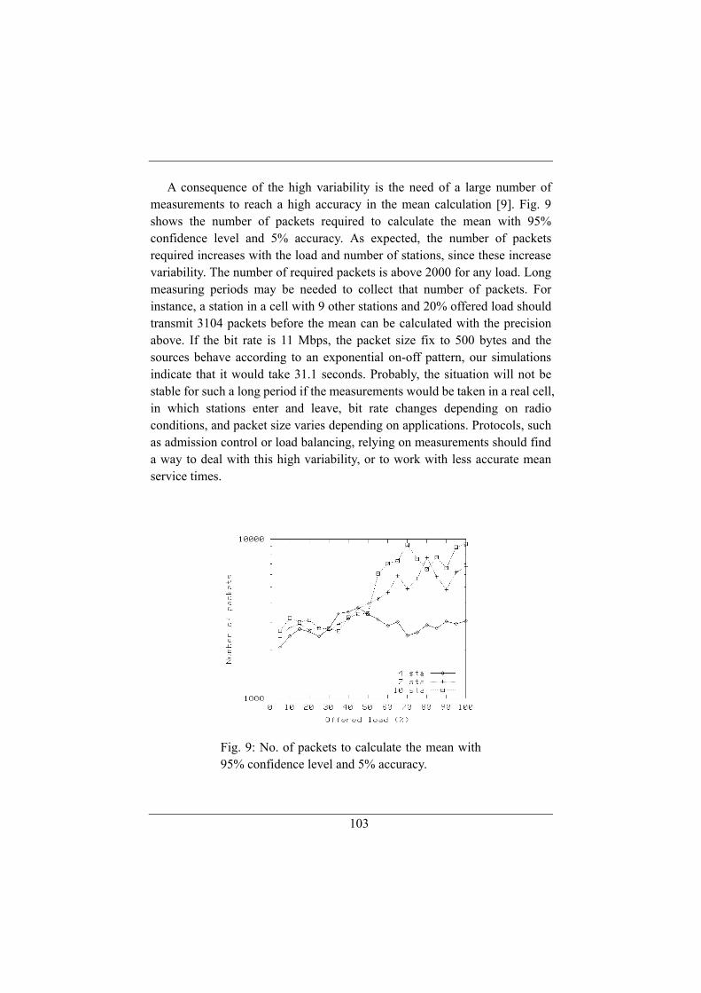
103

A consequence of the high variability is the need of a large number of measurements to reach a high accuracy in the mean calculation [9]. Fig. 9 shows the number of packets required to calculate the mean with 95% confidence level and 5% accuracy. As expected, the number of packets required increases with the load and number of stations, since these increase variability. The number of required packets is above 2000 for any load. Long measuring periods may be needed to collect that number of packets. For instance, a station in a cell with 9 other stations and 20% offered load should transmit 3104 packets before the mean can be calculated with the precision above. If the bit rate is 11 Mbps, the packet size fix to 500 bytes and the sources behave according to an exponential on-off pattern, our simulations indicate that it would take 31.1 seconds. Probably, the situation will not be stable for such a long period if the measurements would be taken in a real cell, in which stations enter and leave, bit rate changes depending on radio conditions, and packet size varies depending on applications. Protocols, such as admission control or load balancing, relying on measurements should find a way to deal with this high variability, or to work with less accurate mean service times.

Fig. 9: No. of packets to calculate the mean with 95% confidence level and 5% accuracy.

104

The high variability and skewed distribution of the service time makes it interesting to look at upper bounds for the service time of the packets rather than mean values. The cumulative distribution function (CDF) of the service time shows the probability that the service time is lower than a certain probability. Fig. 10, Fig. 11 and Fig. 12 present CDFs for low load (15% offered load) and high load (60% offered load) for different number of stations, bit rates, and packet sizes respectively. In low load, most of the packets (approximately 70%) experience a service time smaller than the average, while some of the packets (approximately 5%) experience a service time larger than twice the mean. In high load, the percentage of packets below the mean reduces, but the amount of them that are twice as large as the mean increases.

Low load

High load

Fig. 10: Service time’s CDF for different no. of stations.

Low load

High load

Fig. 11: Service time’s CDF for different bit rates.

105

Low load

High load

Fig. 12: Services time’s CDF for different packet sizes.

Fig. 13: Comparison of the 95-percentile and mean MAC service time in non-saturation.

106

Some applications with strict requirements on each packet’s delay would benefit from estimating the delay with a high percentile; for instance, if the 95-percentile is used, the application will only loose 5% of the packets due to late arrival. Fig. 13 and Fig. 14 show the 95-percentile compared to the mean service time versus offered load for non-saturation and saturation. The 95-percentile is at least double the mean in non-saturation, and there are larger differences in saturation. Fig. 13 indicates that admission control can be used to keep the service time low.

6. ANALYSIS OF CORRELATION

This analysis aims at discovering if the service time of a packet can be calculated from the service time of previous packets. This is possible if there is some correlation between the service times of the packets in a flow. This can be detected with the autocorrelation plot [10]. Fig. 15 shows this type of plot for lags of 1 to 100 in low load. The parameters were 10 stations, packets of 500 bytes and bit rate 2 Mbps. Other parameter values with different loads resulted in similar plots.

The autocorrelation plots contain three horizontal reference lines. The middle one is at zero. The other two are 99% confidence bounds. Since almost all autocorrelations fall within the 99% confidence limits and there is no visible pattern in the plot, the data is random; there is no significant

Fig. 14: Comparison of the 95-percentile and mean MAC service time in saturation.

107

autocorrelation. Therefore, the service time of a packet cannot be calculated from the service time of previous packets.

7. CONCLUSIONS

We have studied the IEEE 802.11 MAC service time via statistical analysis of simulations. Our findings complement existing information from analytical models by providing packet level information for small number of stations. Three different studies were reported. The analysis of location showed that the service time distribution is skewed. The mean and median can be use as typical values; the mode is less interesting because the distribution is multi-modal for medium and high loads. Since the mean is the most common choice, we have shown how it varies with the offered load using the number of stations, bit rate and packet size as parameters. In all cases, the mean presents a quick transition from low values for non-saturation to high values in saturation. The parameters change the offered load at which the transition occurs. Higher bit rates and smaller packets make the transition occur at lower loads, while the number of stations only affects the mean value in saturation. The analysis of variability showed a high spread of the service time around the mean for non-saturation. The variability increased with the load for the three parameters under study. Due to the high variability, we argued that applications with strict requirements on per packet delay would

Fig. 15: Autocorrelation of the MAC service time for low load and 10 stations.

108

benefit from using the 95-percentile instead of the mean as indicator of the expected delay. We also indicated that measuring an accurate mean value in a real cell might be impossible due to the large number of packets required. Finally, the analysis of correlation showed no significant autocorrelation in the service time of the packets in a flow. Hence, the service time of a packet cannot be predicted from the service time of previous packets.

The starting point for this study was the modeling work that has been presented recently. We conclude that models, which are valid only in saturation and for a high number of stations, provide only worst case measures and give limited insight of the performance of wireless LANs. We also conclude that the arithmetic mean might not be a suitable metric for the performance of a WLAN cell due to the high variability. However, if admission control is provided in the cell to limit the load below saturation, then the performance is good and practically invariable with respect to the system parameters considered herein. The main issue in designing such a control mechanism is to determine the cutoff point for the load since this decision level is determined by the transmission bit rates of the stations as well as the characteristics of the offered load with respect to packet arrival patterns and packet size distributions. A promising technique is to use probing for distributed admission control [8].

REFERENCES [1] P. Chatzimisios, A.C. Boucouvalas, V. Vitsas, “Performance analysis of

IEEE 802.11 DCF in presence of transmission errors”, in Proc. of IEEE ICC 2004, pp. 3854 – 3858, June 2004.

[2] Giuseppe Bianchi, “Performance Analysis of the IEEE 802.11 Distributed Coordination Function”, IEEE Journal on Selected Areas in Communication, March 2000.

[3] Y.C. Tay and K.C. Chua, “A capacity analysis for the IEEE 802.11 MAC protocol”, Wireless Networks, vol 7, pp 159-171, Kluwer Academic Publisher, 2001.

[4] Marcelo Carvalho and J.J. Garcia-Luna-Aceves, “Delay analysis of IEEE 802.11 in single-hop networks”, in Proc. of the 11th IEEE ICNP’03, 2003.

[5] A. Banchs, “Analysis of the distribution of the backoff delay in 802.11 DCF: a step towards end-to-end delay guarantees in WLANs”, in Proc of QoFIS 2004, Barcelona, Spain, 2004.

109

[6] Omesh Tickoo and Biplab Sikdar, “A queuing model for finite load IEEE 802.11 random access MAC”, in Proc. of IEEE ICC’04, Paris, France, June 2004.

[7] Bo Li and Roberto Battiti, “Analysis of the IEEE 802.11 DCF with service differentiation support in non-saturation conditions”, in Proc. of QoFIS 2004, Barcelona, Spain, 2004.

[8] Hector Velayos, Ignacio Mas and Gunnar Karlsson, “Distributed admission control for WLANs”, submitted to IEEE Network, special issue on WLANs: QoS and resource management, notification March 1st, 2005.

[9] R. Jain,The Art of Computer Systems Performance Analysis. Techniques for experimental design, measurement, simulation, and modeling, John Wiley & Son Inc., 1991.

[10] NIST/SEMATECH e-Handbook of Statistical Methods, Dec. 2004, http://www.itl.nist.gov/div898/handbook/.

[11] Matthew Roughan and Oliver Spatscheck, “What Does the Mean Mean?”, in Proc. of International Teletraffic Congress (ITC) 18, 2003.

111

PAPER F: MULTI-RATE PERFORMANCE INDEX FOR

WIRELESS LANS

113

Multi-rate performance index for wireless LANs

Hector Velayos and Gunnar Karlsson KTH, Royal Institute of Technology,

{hvelayos,gk}@kth.se

Published in Proceedings of IEEE PIMRC 2004, Barcelona, Spain, Sept. 2004

Abstract—The throughput per access point has been used as the main

figure of merit in performance characterization of wireless LANs. The usefulness of throughput as a performance measure is limited because low throughput can be produced by either low offered traffic or by radio conditions that limit the data rates. In this paper, we propose the Multi-rate Performance Index as an additional figure of merit to characterize the performance of wireless LAN cells. It represents which bit rates are used in the cell, and therefore it identifies cells whose throughput is limited by radio conditions rather than offered traffic. We include several measurements in real cells to illustrate its utility in performance analysis.

Keywords—Wireless LAN, performance, metric

114

I. INTRODUCTION

The characterization of the usage of wireless LANs (WLAN) is becoming an important topic. With an increasing number of wireless LANs deployed at universities, companies and public spaces, WLAN operators are interested in analyzing how these networks perform. The figure of merit commonly used is the throughput per access point (AP).

Published studies on wireless LAN performance such as [1] and [2] report large differences in throughput among APs, as well as for the same AP at different times. However, these studies fail to explain the reasons for unexpected low throughput levels. Sometimes the number of users is given as an indication of the cell load, but Balachandran et al. showed that throughput and number of users are not correlated [1]. In their measurements, they found WLAN cells with many users and low throughout and vice versa. Their explanation is based on the user behavior rather than the number of users. At some places, users connect only to browse and read email, while at other places they make large backups. Although this explanation is plausible, it is also possible that the location of the access point with respect to user’s terminals or the radio condition do not permit to use the higher bit rates of WLANs. Terminals would be transmitting at the basic rates and the throughput would not reach the expected levels. Therefore, throughput and number of users are not enough to assess the performance of wireless LANs.

We propose a new figure of merit called Multi-rate Performance Index (MPI). It is a complementary figure to throughput that measures the bit rates used in a WLAN cell. It provides information about the bandwidth perceived by users, which mainly depends on their position with respect to the AP. It is an important index because it permits to assess whether each cell is been used to its fullest capacity or it is limited by radio conditions.

The application of the MPI is not limited to performance analysis. It can also be used in load balancing [3]. Instead of distributing stations evenly among APs, station can be distributed to maximize the MPI of the cells. This would maximize the capacity of the wireless LAN since each cell would operate at its maximum possible bit rates for the given stations and environment. Admission control is another possible area of application. For instance, the admission policy could state that stations are accepted to a cell if they do not severely reduce the current MPI. This would prevent the IEEE 802.11b performance anomaly presented by Heusse et al [4], since stations

115

operating at low bit rates will not share cell with stations transmitting at the higher bit rates.

The rest of the paper is organized as follows. Section II presents the definition of the Multi-rate Performance Index and its characteristics. Section III describes how to measure it. Section IV analyzes several measurements in real cells. Section V closes the paper summarizing the main findings.

II. MULTI-RATE PERFORMANCE INDEX

An index to measure the bit rates used in wireless LAN cells must meet several requirements. Its value must be contained in a finite range, with the minimum and maximum values corresponding to all frames transmitted at the lowest and highest bit rates respectively. It must be measured on each cell. It must permit comparison between cells with different radio interfaces (e.g. IEEE 802.11a vs. IEEE 802.11b). It must be computed only for successfully transmitted data frames. Control and management frames should be excluded because they are transmitted at fixed bit rate. Finally, it should be easy to measure with passive methods, i.e. without generating additional traffic.

We propose to define the Multi-rate Performance Index for a wireless LAN cell as follows:

∑

∑

=

== N

ii

N

iii

pB

pb

1

1MPI (1)

where N is the number of bit rates supported by the radio interface, bi is the bit rate number i in megabits per second, pi is the number of data frames sent at bit rate bi, and B is the highest supported bit rate in megabits per second.

For instance, IEEE 802.11b cells feature four bit rates (1 Mbps, 2 Mbps, 5.5 Mbps, 11 Mbps), so their MPI would be:

)(11115.521

MPI115.521

115.52180211b pppp

pppp++++++

= (2)

116

The MPI value given in Eq. 1 is undefined when there are no data frames transmitted during the measured interval. In this case, we define the MPI to be zero.

Our definition of the MPI meets all the requirements stated above. The values of MPI vary between 0 and 1. MPI is zero when there were no data frames transmitted during the measured interval. Otherwise, the MPI’s minimum value is the ratio between the minimum and maximum bit rates and it is reached when all data frames were transmitted at the minimum bit rate. The MPI’s maximum value is 1, achieved when all data frames were transmitted at the maximum bit rate. Table 1 shows the minimum and maximum MPI values for different wireless LAN standards in the case that at least one data frame was transmitted.

Table 1

Extreme MPI values for different WLAN standards when at least one data frame was transmitted during the measuring interval

MPI Min Max

IEEE 802.11a 0.11 1

IEEE 802.11b 0.09 1

IEEE 802.11g1 0.02 1

IEEE 802.11g2 0.11 1 1 IEEE 802.11b compatibility enabled 2 Native mode

We have decided to use the number of frames rather than the number of bytes transmitted at each bit rate in the calculation of the MPI because the index should reflect the bit rates that are used in the cell. Each frame represents a successful transmission at its bit rate. The amount of bytes that were transmitted is already reflected in the throughput.

The value of the MPI is easy to interpret. Values close to one are proper indicators of a well-working cell. AP and stations are able to use the highest bit rate most of the times. MPI values close to the minimum indicate that bad radio channel conditions are limiting the usable bit rates. If interferences can

117

be discarded as the reason, then a low MPI is a signal of a badly located AP with respect to the stations’ position. Nevertheless, a low MPI does not necessarily mean that there is a better location. It only means that the current location is not very appropriate.

The MPI can also be used to estimate the actual capacity of a cell. Multiplying the measured MPI by the highest bit rate supported, the average bit rate per frame can be obtained. This would be the actual capacity of the cell since it can be assumed that stations will always try to transmit at the fastest bit rate without errors. The capacity calculated in this way can be compared to the throughput to estimate the cell load.

A particularly interesting application of the MPI is comparing the efficiency of IEEE 802.11a and 802.11g cells for a given location. Both feature the same set of bit rates, but operate on different bands, so it can be expected a difference in performance. But throughput measurements do not indicate which one performs better, particularly for low levels of offered traffic. Comparing the MPI values, it can be determined in which one stations operate at higher bit rates.

In the same way as the throughput, the MPI must be measured over time intervals. The smaller the interval, the higher the influence of each frame’s bit rate in the MPI. Large intervals including many frames produce MPI values closer to its average.

The last requirement for the index was that it should be easy to measure with passive methods. The MPI only requires recording the number of frames and their transmission bit rate. The AP can store this information because all frames in the cell must cross it. Frames arriving from stations contain the used bit rate in the radio header, and the bit rate of frames leaving to stations is selected at the AP. This can be considered a passive measurement method because the existing traffic is never disturbed. Alternatively, stations can compute the cell’s MPI provided that they can receive all transmitted frames.

III. MEASUREMENT TECHNIQUE

Access points currently record statistics about the traffic in the cell for different reasons. Some statistics need to be reported via SNMP such as the number of transmitted frames, while others are used internally. For instance, APs adjust the transmission bit rate by checking whether previous frames

118

were transmitted successfully at their bit rates. Therefore, APs could calculate the MPI without noticeably increasing their computation load.

However, commercial APs cannot be modified at that level, so we have used a different approach to measure the MPI in existing cells. A laptop with a wireless LAN interface was located next to the access point. It executed Linux and the HostAP driver [5]. This driver features a mode called monitor that allows the laptop to receive all frames in the radio channel including the MAC and radio headers. These headers contain enough information to calculate the MPI. We wrote a program [6] that collects and analyzes all frames in the radio channel to calculate the MPI. In short, it records the transmission of each data frame and waits for its acknowledgement. If an acknowledgement confirms the correct reception of the frame, it recalculates the MPI considering the frame contribution. Otherwise, it discards the information about the frame. The position of the monitoring PC next to the AP guarantees that it receives all frames in the cell.

Figure 1 presents preliminary measurements of the MPI in an IEEE 802.11b cell using the method described above. The upper plot shows the MPI computed over periods of 1 second in two cases. In the first case, all data frames were included, while in the second one broadcasted data frames were excluded. The lower plot shows the number and bit rate of the data frames transmitted grouped by seconds.

IEEE standards for WLAN mandate that broadcasted data frames must be transmitted at the highest basic rate so that all stations can receive them. In

Figure 1: Influence of broadcasted data frames in MPI value

119

the case of a 802.11b cell, this bit rate is 2 Mbps. The upper plot shows the influence of the broadcasted traffic in the MPI value. In general, the MPI is lower if broadcasted frames are included, because their bit rate is smaller than the maximum bit rate of regular frames.

Since the bit rate of broadcasted frames is fixed, we suggest excluding them from the MPI calculation. Thus, the rest of the measurements in this paper will not include any broadcasted data frame.

IV. MEASUREMENTS AND ANALYSIS

We have performed several MPI measurements in IEEE 802.11b cells of a campus wireless network using the method described above. All measurements were made in cells with real users and several stations. The MPI and throughput was calculated every second. We report here three representative examples of our measurements.

Figure 2 presents the measurement of MPI and throughput in a high-performance cell during 5 minutes. In this case, most of the frames are transmitted at the maximum bit rate (i.e. 11Mbps), thus the index is close to its maximum. Occasional frames transmitted at lower bit rates due to varying channel conditions prevent the MPI from reaching its theoretical maximum value of one.

Figure 2 also shows that throughput and MPI are uncorrelated figures of merit. The throughput plot exhibits the typical profile of a cell with several

Figure 2: MPI and throughput in a high-performance cell

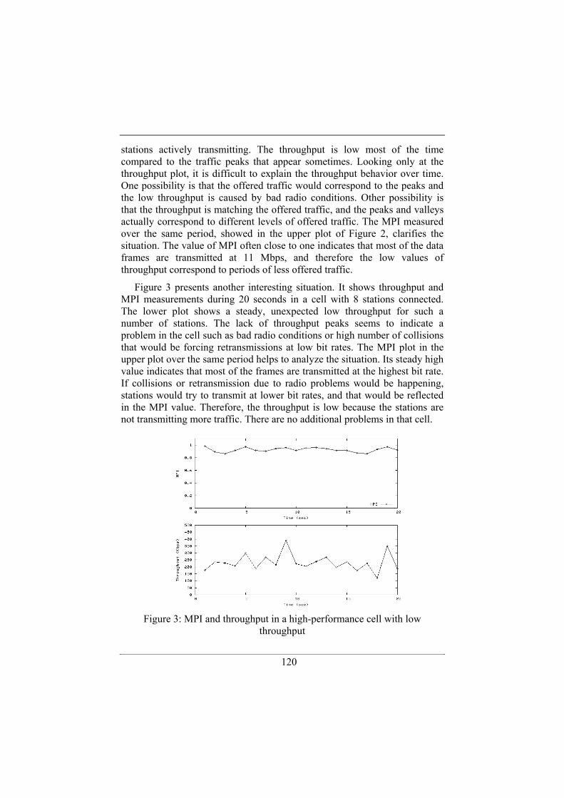
120

stations actively transmitting. The throughput is low most of the time compared to the traffic peaks that appear sometimes. Looking only at the throughput plot, it is difficult to explain the throughput behavior over time. One possibility is that the offered traffic would correspond to the peaks and the low throughput is caused by bad radio conditions. Other possibility is that the throughput is matching the offered traffic, and the peaks and valleys actually correspond to different levels of offered traffic. The MPI measured over the same period, showed in the upper plot of Figure 2, clarifies the situation. The value of MPI often close to one indicates that most of the data frames are transmitted at 11 Mbps, and therefore the low values of throughput correspond to periods of less offered traffic.

Figure 3 presents another interesting situation. It shows throughput and MPI measurements during 20 seconds in a cell with 8 stations connected. The lower plot shows a steady, unexpected low throughput for such a number of stations. The lack of throughput peaks seems to indicate a problem in the cell such as bad radio conditions or high number of collisions that would be forcing retransmissions at low bit rates. The MPI plot in the upper plot over the same period helps to analyze the situation. Its steady high value indicates that most of the frames are transmitted at the highest bit rate. If collisions or retransmission due to radio problems would be happening, stations would try to transmit at lower bit rates, and that would be reflected in the MPI value. Therefore, the throughput is low because the stations are not transmitting more traffic. There are no additional problems in that cell.

Figure 3: MPI and throughput in a high-performance cell with low

throughput

121

Finally, Figure 4 contains measurements of MPI and throughput in a cell with performance problems. The cell has two stations offering an aggregated, average throughput of roughly 200 kbps. The lower plot displays the throughput. An interval over 20 seconds is clearly visible in which the throughput drops to almost zero. The MPI plot in the upper part of Figure 4 indicates that the cause is a temporary problem with the radio channel. The MPI shows that the frames transmitted during the low throughput period used lower bit rates. The stations were trying to overcome the radio fading by reducing their bit rates. Interestingly, the peaks in the MPI show that the stations’ policy was to try to increase the bit rate to check whether the bad radio channel conditions had subsided.

V. CONCLUSIONS

Wireless LANs feature multi-rate radio interfaces. We have shown that the performance analysis of the cells is limited if the throughput is the only figure of merit considered. We suggested the Multi-rate Performance Index to improve the performance analysis. It indicates which bit rates are actually used, allows the comparison between cells of different types (e.g. IEEE 802.11a and 802.11b) with respect to their channel usage efficiency, and permits to calculate the actual cell capacity if the maximum bit rate is known. In combination with existing figures of merit such as the throughput,

Figure 4: MPI and throughput in a low-performance cell

122

it permits a better understanding of wireless LAN cell’s performance. The MPI can also be useful in other areas such as load balancing or access control.

REFERENCES

[1] Anand Balachandran, Geoffrey M. Voelker, Paramvir Bahl, P. Venkat Rangan, “Characterizing User Behavior and Network Performance in A Public Wireless LAN”, in Proceedings of ACM SIGMETRICS 2002, 2002.

[2] David Kotz and Kobby Essien, “Characterizing Usage of a Campus-wide Wireless Network”, Technical Report TR2002-423, Dartmouth Computer Science Technical Report, March 2002.

[3] Hector Velayos, Victor Aleo and Gunnar Karlsson, “Load balancing in overlapping wireless LAN cells”, in Proceedings of IEEE ICC 2004, Paris, France, June 2004.

[4] Martin Heusse, Franck Rousseau, Gilles Berger-Sabbatel, Andrzej Duda, “Performance Anomaly of 802.11b”, in Proceedings of IEEE INFOCOM 2003, 2003.

[5] HostAP Linux driver for Prism-based wireless LAN cards, http:// http://hostap.epitest.fi/

[6] MPI measurement tool, available to download from http://www.imit.kth.se/~hvelayos/software

123

PAPER G: PERFORMANCE MEASUREMENTS OF THE

SATURATION THROUGHPUT IN IEEE 802.11 ACCESS POINTS

125

Performance measurements of the saturation throughput in IEEE 802.11 access points

Enrico Pelletta and Hector Velayos

KTH, Royal Institute of Technology 16440 Kista, Sweden

[email protected] [email protected]

Published in Proceedings of 3rd Intl. Symposium on Modeling and Optimization in Mobile, Ad Hoc, and Wireless Networks, Trentino, Italy,

April 2005 Abstract—Performance measurements of IEEE 802.11 access points

provide important information for networking research and network management. In this paper, we present an active measurement method to determine the maximum saturation throughput of wireless LAN access points. The saturation throughput is achieved when there always is a frame ready to transmit, and it reaches the maximum for optimal transmission conditions. We use the proposed method to measure and analyze the performance of five IEEE 802.11b access points. The results show the strength of our method and identify performance characteristics of commercial access points. The analysis produces the following results. The maximum saturation throughput shows significant differences between models. Increasing the offered load to the access point’s Ethernet interface does not always increase the throughput; a few access points present a downlink throughput reduction when the offered load exceeds their bridging capabilities. Some access points exhibit better performance in certain orientations.

Index terms—measurement, throughput, wireless LAN

126

A. INTRODUCTION Performance studies of IEEE 802.11 access points are becoming

increasingly important since it is the predominant choice for high-speed wireless access to Internet. Performance analysis based on mathematical models is crucial for protocol design and parameter adjustments. Several studies are available focusing in different aspects such as throughput, delay or back off duration. The main limitation of these studies is the simplification of the protocol operation necessary to make the problem suitable for mathematical analysis: mathematical models cannot consider protocol details such as the needs for regular beacon transmissions. IEEE 802.11 performance analysis based on simulations complement the mathematical analysis. Simulations often include complete implementations of the protocols and hence, provide results that are more realistic. They permit the study of the protocol for different traffic patterns and user behaviors. However, simulations are not equivalent to real life measurements. They need to include some simplifications in areas such as hardware performance, radio propagation or terrain modeling.

Performance measurements are necessary to assess the characteristics of real devices. These measurements are particularly useful for network planning. In this paper, we present our work to characterize the performance of IEEE 802.11 access points (AP). In particular, we focus on throughput as the main figure of merit. Previous works had studied throughput as a function of range [1][2]. The environment used for the measurement is the key factor in these works. The same experiment with an access point in two different places may yield completely different results. According to our previous work, the results are also different if the wireless stations change their position during the experiment [11]. In order to have repeatable experiments, we focus our measurements on the access point and try to eliminate the influence of the environment on the results. We chose the saturation throughput as the figure of merit to characterize the performance of access points. The saturation throughput is achieved when the access point always has a frame ready to be transmitted, and it reaches the maximum for optimal transmission conditions and appropriate offered traffic. The maximum saturation throughput is interesting because it represents the upper bound for the access point’s throughput.

The first contribution in this paper is a methodology to reach and measure the maximum saturation throughput of any 802.11 access point. The proposed procedure includes the testbed setup, the software tools and the mathematical support for processing the results. All these aspects were investigated in order to define a unique and repeatable test procedure. The main effort was invested in finding the factors that limit the access point

127

performance. The instant saturation throughput has a too large variance to be significant, even in optimal conditions. The main reason is that the time between consecutive frames generated from an AP varies due to internal performance limitations. Another less frequent reason is that some frames are transmitted at lower bit rates than the maximum one. Instead of a single measurement, we use the mean of a set of saturation throughput samples as the figure of merit. The test procedure allows computing this mean with a defined confidence level and accuracy.

The second contribution is the measurement of the maximum saturation throughput in five IEEE 802.11b access points obtained following our proposed method. The purpose of the measurements was to validate our methodology, and to identify some performance characteristics of current access points. The analysis of the measurements produced the following results. The maximum saturation throughput shows significant differences between models. Increasing the offered load to the access point’s Ethernet interface does not always increase the throughput; a few access points present a downlink throughput reduction when the offered load exceeds their bridging capabilities. Finally, despite that all access points are equipped with omni-directional antennas, some of them exhibits better performance at certain orientations.

The rest of the paper is organized as follows. Section B introduces the maximum saturation throughput and the statistical framework required for its measurement. Section C describes the challenges and our solutions to measure the maximum saturation throughput. Section D explains the measurement procedure. Section E shows the results from our measurements. Section F provides a detailed analysis of each measured AP’s behavior. Section G closes the paper summarizing the main findings.

B. MAXIMUM SATURATION THROUGHPUT

Throughput can be generally defined as the ratio of received data to the time necessary to transmit it. Since the goal of our measurements is the AP throughput, we consider received data to be the payload of the link-layer frames that are successfully received by the destination node.

The AP throughput depends on the offered traffic. In this paper, we restrict our work to the saturation throughput. The AP's saturation throughput is the throughput when the AP always has a packet ready to be transmitted. This throughput reaches a maximum in absence of limiting factors such as bad radio conditions.

We chose to restrict our investigation to the maximum saturation throughput for several reasons. First, the maximum saturation throughput is an important performance index. It provides an absolute limit on the

128

throughput of an AP. Second, the conditions to maximize the saturation throughput can be precisely defined. Therefore, it is possible to recreate the same test environment almost everywhere at any time in order to repeat the experiments. Often, it is not possible to replicate the measurements of other performance indexes, for instance throughput versus range, because different environments generate different results. Third, measuring the maximum saturation throughput means that the AP is forced to work at its full capacity. This condition magnifies several implementation-specific behaviors, both good and bad. Fourth, our experiments indicate that a device that shows good performance in our particular conditions produces the same level of performance under different conditions. This kind of behavior has been observed on various devices, and previously reported in [3][4].

Another important aspect of throughput measurements is the duration of the measurement. The throughput varies over time despite the optimal transmission conditions. The reasons include variable time between consecutive frames generated from an AP due to internal performance limitations, and transmission of some frames at lower bit rates than the maximum one. The traditional approach is to use a long measuring interval to reduce the impact of temporary throughput alterations. We found this solution limited because it hides information on the AP behavior. Instead, we collect a number of consecutive, short samples of the throughput and characterize the throughput via the mean and standard deviation of the sample set. The mean indicates the expected throughput, while the standard deviation provides information about the stability of the AP. The maximum and minimum sample values are also provided.

We need to determine the sample duration. The shorter the sample duration, the better temporary throughput fluctuations are reflected. The extreme case would be to generate a throughput sample after the reception of each frame. Fig. 1 shows the throughput of an access point measured in this way. The periodic throughput reductions in the figure correspond to samples including a beacon transmission in addition to one data frame. Since the beacon must be broadcast at 2 Mbps every 100 ms and it does not contain data payload, it reduces the throughput of some samples. This would also affect the mean throughput computed over a few packets. To address this problem, we sample the throughput every 150 ms, which roughly includes 100 packets per sample. This number of packets per sample guarantees that the effect of the beacon can be neglected. The non-periodic throughput reductions in Fig. 1 are due to the AP’s behavior.

The number of samples used to calculate the mean throughput determines the accuracy of the result and its confidence level. The accuracy is expressed as an interval around the measured value in which the real value lays with

129

the probability given by the confidence level. The number of samples (Ns) to reach a given accuracy can be calculated as follows [6]:

=

2100rx

zNs σ (1)

where x and σ are the mean and standard deviation, respectively, of the throughput samples, r is the desired accuracy in percent, and z is the quantile of the unit normal distribution. This value depends on the selected confidence level. We will use a 95% confidence level and z will therefore be 1.960. The symbol ⋅ denotes the ceiling of the argument.

Unfortunately, it is not possible to use Eq. 1 to determine the number of required samples because the throughput's mean and standard deviation of an AP under saturation are unknown in advance. Instead, we determine a lower bound for the necessary number of throughput samples to collect during the experiments to reach the desired accuracy. Eq. (1) shows that the necessary number of samples is proportional to the square of the coefficient of variation (C.o.V) (ratio of the standard deviation to the mean). According to our preliminary tests, the C.o.V. is always below 1 in our measuring conditions (i.e. variations are small due to the optimized test bed), so we use a C.o.V. equal to 1 for the lower bound of the number of samples. Since the theoretical maximum value of the C.o.V. for the 802.11 AP's saturation throughput is higher than 1, it will always be necessary to verify that the C.o.V. was below 1 after the measurements. Our assumption might fail when measuring the throughput of devices with extremely low and unstable

Fig. 1 Instantaneous throughput of an access point. Each throughput sample

contains one frame.

130

performance. However, we consider such behavior a failure of the tested AP, to be treated as an exception.

Assuming the C.o.V. is 1 and using a 95% confidence level, the number of necessary samples to collect is equal to

=

2196r

Ns (2).

Eq. (2) shows the tradeoff between number of samples and accuracy. Increasing the accuracy (i.e. reducing r) increases the measurement duration because a larger number of samples is required. We want to reach a 3% accuracy for our measurements, which means that at least 4268 samples of 150 ms are required. This yields an estimated test duration of roughly 11 minutes for an IEEE 802.11b AP.

Finally, it is necessary to consider the data stream direction when measuring the throughput. We measure the downlink throughput, i.e. from the access point to the stations, because it is the most demanding for the access point. If there are performance limitations in the AP, they are more visible in the downlink throughput than any other stream direction. One practical advantage of the downlink throughput is that it is independent of the number of stations in the cell and the performance of their wireless card. This simplifies the set up for the measurements.

The uplink throughput is less interesting to characterize the AP’s behavior because it is dominated by the stations’ performance. The IEEE 802.11 MAC protocol places all critical operations and decisions in the sender. For instance, the sender chooses the bit rate to transmit each packet depending on its perceived quality of the radio channel. The receiver, the AP in the upstream direction, only acknowledges the reception of the frames within very strict time limits and forwards received frames towards the Ethernet backbone.

We have conducted some experiments to verify this hypothesis. Fig. 2 shows the instantaneous uplink throughput in saturation for two access points. Each dot in the figure corresponds to a throughput sample of 150 ms. During the 30 minutes’ measurements, one wireless stations transmitted WLAN packets of 1500 bytes to a destination in the Ethernet backbone as fast as possible.

131

Although these APs present different behavior in downlink as shown in Table I, they reach the same uplink throughput as indicated by the virtually equal insets (a) and (b) in Fig. 2. Other experiments with the rest of APs in Table I resulted in similar plots. This confirms that the station’s performance is the key in uplink throughput rather than the AP. It also confirms that the operations at the APs on incoming packets do not affect the uplink throughput. We have however observed differences in the uplink throughput

(a)

(b)

Fig. 2 Instantaneous uplink throughput in saturation for two access points: (a) Cisco AIR 1200, (b) Avaya RGII.

132

when using different wireless LAN cards and drivers in the station. We have not analyzed this further since it is outside the scope of this paper.

We have also verified that the uplink throughput depends on the number of stations as suggested in [5]. Fig. 3 shows the mean uplink saturation throughput and confidence intervals of the Cisco Air 1200 AP. Six sessions are reported, three with one station and three with two stations. In line with theoretical results, the saturation uplink throughput increases when adding a second station. Similar experiments showed that the second station does not affect the downlink throughput.

Another alternative would be to measure saturation throughput using simultaneous uplink and downlink streams. This is not an interesting option. The performance problems of some APs result in the channel to be idle for short periods. These periods are filled by transmissions from the wireless station and are thus hiding the performance problems.

C. CHALLENGES TO MEASURE THROUGHPUT

We focus our work on measuring and analyzing the maximum saturation throughput of the APs. Therefore, we need to enforce all necessary conditions in order to maximize the saturation performance of 802.11 APs. The first condition is to use an environment that facilitates good radio transmissions. We use short distances between the wireless nodes, but longer than the manufacturer’s minimum distance recommendation (typically 1 meter). We scan the radio channel during the measurements to discard measurements affected by noise or interferences. The optimal test

Fig. 3. Mean uplink saturation throughput and confidence intervals of the

Cisco AIR 1200 access point.

133

environment would have been an open, outdoor space with no obstacles, but it was not feasible. Hence, we used a small and closed room to minimize the influence of multi-path transmissions [7].

The characteristics of the IEEE 802.11 medium access- control protocol impose additional constraints to maximize the AP's saturation throughput. The IEEE 802.11 standard defines two different modes for the medium access-control protocol: basic access and RTS/CTS (Request-To-Transmit/Clear-To-Transmit). In order to achieve the maximum saturation throughput, we use the basic access mechanism. Kamerman and Aben showed that the basic access provides higher performance in good radio conditions [8]. The throughput also depends on the packet size. Under optimal radio conditions, the larger the packets are, the higher the throughput is [5][9]. Thus, the data streams must be made of IP packets of 1500 bytes. This is the largest possible packet size when using an AP connected to an Ethernet backbone.

Some commercial IEEE 802.11 APs provide the administrator with the possibility to customize the configuration for the deployment scenario by selecting alternative profiles. A large set of options is available and may produce different performance under our conditions. Often the set of possible AP options is too large to be extensively examined. Thus, we suggest using the vendor’s recommend configuration that guarantees full interoperability between different 802.11 implementations.

Another factor to consider is the orientation of the AP with respect to the receiving station. All APs are equipped with omni-directional antennas. But our measurements showed that the performance of some APs is reduced at certain orientations. Fig. 4 shows such an example. Fig. 4-a plots the instantaneous saturation throughput of an IEEE 802.11b access point in saturation. The samples were collected every 150 ms during one hour. The throughput is unexpectedly low for such an AP capable of reaching 11 Mbps. Fig. 4-b shows the results of the same experiment after rotating the AP 180 degrees. Throughput’s samples are still lower than expected but higher than before. Our measurement procedure includes a preliminary test to identify this type of behavior and find a non-limiting orientation for the measurements.

An unexpected problem was the influence of the offered load in the AP performance. Theoretical studies indicate that the throughput grows with the offered load until the capacity of the link is reached. Then, increasing the offered load above the channel capacity results in the same maximum throughput. Our measurements indicate that some APs show a different behavior. Their throughput reaches a maximum for certain offered load and then decreases if the offered load continues to grow. Fig. 7 shows the

134

influence of the offered load on the throughput for some access points. These results indicate that it is necessary to find out the offered load that produces the maximum throughput for each AP.

Finally, it is important to determine the time required for the traffic to stabilize. An AP uses the first frames of a new flow to test the channel and choose an appropriate bit rate. Different models use different schemes. Some start sending at the lowest bit rate and increase it on each successful

(a)

(b)

Fig. 4 Influence of the access point’s (AP) orientation on its throughput: (a) throughput of an AP during one minute, (b) same experiment after

rotating the AP 180 degrees.

135

transmission, while others start from the highest bit rate and decrease it on each error. To avoid that these actions affect our measurements, the measurements start some time after the test packet stream begins. In order to determine how much time was needed, we looked at the AP’s throughput measured on every received packet during the first milliseconds of a flow. Fig. 5 presents the results from one IEEE 802.11b. Other APs produced similar plots. Fig. 5 shows that the throughput stabilizes after a small number of packets corresponding to a few milliseconds. The throughput samples with smaller values after 20 ms correspond to samples including a beacon transmission. Looking at this type of plots, we decided to wait for one second before collecting throughput samples. One second provides ample margin for the flow to stabilize.

D. MEASUREMENT PROCEDURE The measurement procedure for each AP can be split into three phases:

set up of the test bed, preliminary measurements, and saturation throughput measurement.

The set up is depicted in Fig. 6. Three computers are necessary to perform the measurements. The Ethernet node is used to generate the test packet stream on the Ethernet link. The wireless node is used to receive the test packet stream on the wireless link. The monitor node records the traffic on the wireless network for later traffic analysis and throughput calculation. The monitor and wireless nodes were collocated at 2 meters distance from the AP. One Ethernet crossover cable is used to transport the test packet stream to the AP, and an independent switched Ethernet network distributes

Fig. 5 Throughput measured after every received frame during the first 200

ms of a new flow in an IEEE 802.11b access point.

136

management information, such as time synchronization between the nodes. In fact, this set up does not require accurate time synchronization because the time stamp of the packets’ arrival is always relative to the monitor node’s clock.

We use open source code for the computers. Red Hat Linux was used as the operating system. The packet stream was generated using an open source tool called MGEN1. This tool can generate and receive UDP/IP streams of packets with a configurable transmission rate and packet size. We use tcpdump2 in order to record the network traffic on the monitor. The link layer and IP headers are stored for data and management frames. The throughput calculation and traffic analysis were done after the measurements using software that we created for parsing the trace files generated by tcpdump3. One piece of software extracts the throughput sample set from the trace files discarding the initial transient and reporting general statistical information (i.e. number of parsed packets, number of beacons). Another software parses the sample set produced before and computes the statistical indexes for the saturation throughput (i.e. mean, standard deviation, maximum and minimum sample values).

The proposed test bed may introduce some measurement errors. A systematic error could be introduced because of different packet propagation time. We assume that packets arrive at the same time to the monitor and wireless nodes because both computers are very close together. Another source of error could be the limited resolution of the packet time stamp. Commercial wireless cards feature a time stamp resolution of a few tens of microseconds. This does not have a significant impact in our case because each throughput sample is 150 ms long.

After the test bed is prepared, the preliminary measurements can be conducted. Their goal is to discover if an AP performs differently depending on its orientation with respect to the receiving station. If this happens, the best orientation needs to be identified. Unfortunately, an exhaustive and accurate investigation would need a very large amount of time and resources. An AP can be turned in an almost infinite number of ways. However, many times the vendor recommends an optimal mounting direction for the AP. Therefore it is always possible to restrict the investigation to the AP rotation around its vertical axis. We recommend to

1 MGEN is available at http://tang.itd.nrl.navy.mil/5522/mgen/mgen_index.html

2 TCPDUMP is available at http://www.tcpdump.org/ 3 This software can be downloaded from

http://www.imit.kth.se/~hvelayos/software.shtml

137

run at least four tests turning the AP 90 degrees around its vertical axis after each test. This procedure does not allow exactly measuring the optimal AP orientation, but only allows discovering the main antenna characteristics and selecting an adequate AP orientation. We recommend to run this test and to use the resulting best AP's orientation for the rest of the measurements.

The final step is to measure the maximum saturation throughput. Since some AP’s saturation throughput depends on the offered load, the AP should be tested with all the possible loads to find the one maximizing the throughput. The only possibility to vary the offered load is to change the packet arrival rate because the test data stream is made of UDP packets of a fixed size (1500 bytes of Ethernet payload). In order to minimize the number of necessary tests, we recommend starting the first test from the highest offered load that can be carried by the wireless link. For instance, 900 packets per second (around 11Mbps) would be the starting load to test an IEEE 802.11b AP, which has a maximum bit rate of 11 Mbps. After the first test session with the highest offered load, the test is repeated decreasing the offered load by 100 packets per second each time. The test is repeated as long as the measured AP throughput increases or until the offered load is completely forwarded by the AP. The highest saturation throughput among all tests is the maximum saturation throughput and it is reached for the corresponding offered load. In the case of different offered loads producing the same AP throughput, the highest of these values is selected as the optimal one.

E. MEASUREMENT RESULTS

We present measurement results to demonstrate the capabilities of the proposed method and to provide information about the behavior of some commercial access points. We report the results corresponding to each of the

Fig. 6 Test bed for measuring the maximum throughput of

an access point.

138

proposed tests: average and standard deviation for the maximum saturation throughput, relation between the offered load and throughput, and influence of the orientation. These results are given for five commercial IEEE 802.11b access points from four vendors including simple models for home usage, and more sophisticated models for large-scale wireless LANs. Additional results from the tests such as uplink saturation throughput and noise levels are given in [10].

Table I presents the saturation throughput for each model. Results in the table include the mean saturation throughput, and its standard deviation, with 95% confidence level and 3% accuracy. The table also shows the maximum and minimum sample values. Each AP was measured under its optimal offered load and orientation.

The saturation throughput presents important differences among models. Model D outperforms all other models. Its saturation throughput is 40% larger that the slowest access point. Per-packet analysis confirmed that the test environment was correct and all frames were transmitted at the maximum bit rate with a negligible number of retransmission for the models A, B and E. The reason for the low throughput in these models was a larger idle time between consecutive frames compared to the model D. These models cannot transmit faster. Model C showed a different problem. It seems to be extremely sensitive to the environmental conditions. Despite our efforts to provide an optimal environment and to optimize the AP test conditions (i.e. optimal orientation and offered load), the device could not maintain a stable bit rate over long time intervals. The packet’s bit rate was alternating between 11 and 5.5 Mbps. Sometimes, the device interrupted the transmission for intervals of around 200 ms without any apparent reason.

Table I Saturation throughput with 95% confidence level and 3% accuracy.

Id. Model Saturation

throughput (Kbps)

Standard deviation (Kbps)

Max. (Kbps

)

Min. (Kbps)

A Avaya RG-II

5158 69 6560 4960

B Orinoco AP 1000

6609 145 6960 5520

C Orinoco AP 2000

6636 612 7120 0

D Cisco Air 1200

7233 251 8480 5520

E Ericsson A11d

5801 132 6720 4480

139

This behavior impacted our measurement, but it seems to be a specific characteristic of this model. No other model experienced the same behavior in our test bed.

Common to all models is a small standard deviation compared to the saturation throughput. This indicates that their behavior is stable. Model C showed a surprisingly high standard deviation for the reasons stated above.

It is important to remember that our measurement procedure assumed that the C.o.V. was below 1. Table I shows that the standard deviation is smaller than the mean for all models. This confirms our assumption.

The measured saturation throughput is smaller than the maximum bit rate (11 Mbps) for two reasons. First, the radio and MAC layer headers are transmitted but not included in the throughput calculation. The received data is the payload of the MAC frames as defined in Sec. B. Second, the MAC protocols imposes an overhead per transmitted frame. The MAC overhead includes the transmission of an acknowledgement at 2 Mbps and some idle periods between transmissions (inter frame space).

Fig. 7 shows the influence of the offered load on the saturation throughput. The offered load is measured as the number of packets arriving to the AP’s Ethernet interface. The size of the packets is the maximum Ethernet frame and 800 packets per second is the maximum rate of the Ethernet interface. The results show two types of behaviors. Some access points, such as models B and D, maintain the saturation throughput when the offered load exceeds their bridging capacities. While others reduce the saturation throughput if overloaded (e.g models A, C, E). The reduction can be significant depending on the models. For instance, model C showed a

Fig. 7 Relation between saturation throughput and offered load.

140

40% decrease of the saturation throughput. This result suggests that wireless LANs using these access points should perform admission control to maintain the offered load within appropriate limits.

Fig. 8 illustrates the effect of four different orientations in the saturation throughput. This test was made with an offered load of 800 packets per second. This value is not optimal for some APs, which explains the low saturation throughput achieved by some of them. The goal was to analyze the influence of the orientation, not to reach the maximum saturation throughput. All access points claimed to feature omni directional antennas. Models A and E showed the expected results. Their saturation throughput does not depend on the orientation. Models C and D were close to this behavior, showing saturation throughput drops of less than 10% for some angles. However, model B experienced significant throughput reduction for the 270 degrees angle. This test was repeated several times with similar results. The most probable reason is an interference created by the shape of the AP’s case or any of the components inside.

F. DETAILED ANALYSIS The goal of our suggested measurement procedure is to obtain the mean

saturation throughput with a given accuracy rather than explaining the differences in performance among APs. However, it is possible to explain the causes for each AP’s performance by looking at the trace files generated during the measurements. In this section, we report the results of such detailed analysis to explain the results shown in the section above.

Fig. 8 Influence of the orientation on saturation throughput.

141

Model A achieved the lowest mean saturation throughput. Fig. 9 shows the instant saturation throughput for model A during our measurements. It also presents the cumulative number of retransmissions.

Fig. 9 and the analysis of the IEEE 802.11 traffic do not show any abnormal behavior during the test that could explain the lower throughput of this model. The AP sends the beacons at regular intervals (102 ms average beacon transmission interval; no detected missing beacons). The number of retransmission at the link layer is low: 0.04% of 802.11 data frames were retransmitted (358 retransmissions over 834165 total packets). No 802.11 management packets were sent. Thus, no RTS/CTS messages, association request/reply, authentication request/reply or probing request/reply were recorded.

The number and distribution of retransmission events and the value of the throughput samples could indicate that this AP only sends data at 5.5 Mbps. To verify this hypothesis, we performed a short downlink test where we captured the radio header of the 802.11 frames to check their bit rate. This test showed that all data frames are sent at 11Mbps, so the hypothesis was not correct. Our conclusion is that the AP cannot transmit packets at a faster rate; therefore, the channel is not used for relatively large fractions of time accounting for the lower throughput.

Fig. 9 Instant saturation throughput in optimal conditions for model A and

cumulative number of retransmissions.

142

Model B achieved a reasonable throughput, but the AP’s orientation has a significant impact on performance. Fig. 10 shows the instant saturation throughput produced by this model with the best and worst AP’s orientations. The 0 degrees position corresponds to the AP’s front side

(a) Orientation of 90 degrees

(b) Orientation of 270 degrees

Fig. 10 Instantaneous saturation throughput as function of the orientation for model B and cumulative number of retransmissions.

143

facing the client. Note the large differences in the number of retransmitted packets between the two cases.

The influence of the orientation on the throughput for model B can be explained by looking at Fig. 10. In the best orientation (90 degrees), the AP

(a) Offered load of 550 packets/s

(b) Offered load of 600 packets/s

Fig. 11 Instantaneous saturation throughput as function of the offered load for model C and cumulative number of retransmissions.

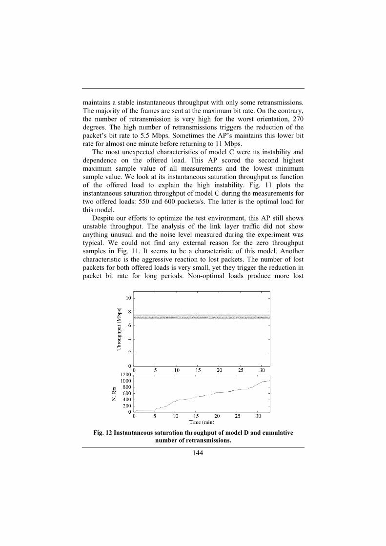
144

maintains a stable instantaneous throughput with only some retransmissions. The majority of the frames are sent at the maximum bit rate. On the contrary, the number of retransmission is very high for the worst orientation, 270 degrees. The high number of retransmissions triggers the reduction of the packet’s bit rate to 5.5 Mbps. Sometimes the AP’s maintains this lower bit rate for almost one minute before returning to 11 Mbps.

The most unexpected characteristics of model C were its instability and dependence on the offered load. This AP scored the second highest maximum sample value of all measurements and the lowest minimum sample value. We look at its instantaneous saturation throughput as function of the offered load to explain the high instability. Fig. 11 plots the instantaneous saturation throughput of model C during the measurements for two offered loads: 550 and 600 packets/s. The latter is the optimal load for this model.

Despite our efforts to optimize the test environment, this AP still shows unstable throughput. The analysis of the link layer traffic did not show anything unusual and the noise level measured during the experiment was typical. We could not find any external reason for the zero throughput samples in Fig. 11. It seems to be a characteristic of this model. Another characteristic is the aggressive reaction to lost packets. The number of lost packets for both offered loads is very small, yet they trigger the reduction in packet bit rate for long periods. Non-optimal loads produce more lost

Fig. 12 Instantaneous saturation throughput of model D and cumulative

number of retransmissions.

145

packets, increasing the number of periods in which the throughput remains at the low level, and hence reducing the mean throughput. An example of this situation is illustrated in Fig. 11. Fig. 11-a plots the throughput and cumulative number of retransmission for a non-optimal offered load of 550 packets/s. It contains twice as many low throughput periods as Fig. 11-b, in which the same experiment is repeated with the optimal offered load.

Model D scored the highest mean saturation throughput of our set of APs. Additionally, it was the AP with the second smallest difference between the maximum and minimum throughput samples, which gives an indication of its high stability. Fig. 12 shows the instantaneous saturation throughput of this model during our measurements and helps to explain its characteristics.

The upper subplot of Fig. 12 confirms the high performance and stability of this model. All throughput samples are closely grouped around 7200 Kbps. There are no visible outliners. Looking at the trace file, we discovered that this model has an aggressive policy for selecting the bit rates. A lost packet does not trigger a reduction in the bit rate, but a retransmission at the same bit rate. Since the AP operates in optimal conditions, this aggressive choice results in high mean throughput.

Model E achieved a modest mean saturation throughput but showed very stable behavior as indicated by a reduced standard deviation and the smallest difference between maximum and minimum throughput samples recorded among all tested models. Fig. 13 shows the instantaneous saturation

Fig. 13 Instantaneous saturation throughput of model E and cumulative

number of retransmissions.

146

throughput of this model and the cumulative number of retransmissions. Model E’s performance shown in Fig. 13 resembles the behavior of model D, but with lower mean throughput. Model E seems to operate a similar policy to model D for bit rate selection of retransmitted packets, but achieves lower throughput due to a higher number of lost packets. The performance of model E’s radio seems to be the limiting factor.

After looking at each model’s behavior, we want to add some findings that affect several of them. Models A, B and C have a common factor: they are different evolutions of the former Lucent Inc. WaveLAN 802.11 products. All of them are based on the same radio implementation. Their architecture consists of a main unit that changes depending on the AP model, and a PCMCIA wireless card that includes the 802.11b specific hardware (i.e. MAC protocol chipset, radio modem and antenna). The wireless card used by these three APs is the same and can be exchanged between different units. The card was an out-of-the-self former Lucent, now Proxim/Orinoco or Avaya, IEEE 802.11b client card.

Additional conclusions can be drawn from our measurements knowing that the three models use the same radio interface. Model B and C showed dependence of the performance on the orientation, while model A did not. This could be expected because model B and C use the same chassis, whereas model A has a different one with the wireless card mounted in a different position.

The differences in mean saturation throughput cannot be attributed to the radio interface, but to the different implementations of the AP’s. Models B and C produce the same downlink maximum saturation throughput, but they have opposite behaviors in response to increasing offered loads. Although model C has the best hardware according to the manufacturer’s specifications, model B handles better the overload of its Ethernet interface. Model A’s lower performance can be justified by its simpler hardware.

Another reason for differences is that the three models run different firmware. Some versions of the firmware implement different policies or offer different default configurations. Consequently, they produce different results under the same test conditions. In particular, the AP’s responses to transmission errors were very different. Model B seems to be much more sensitive to radio transmission errors than the other APs. The performance degradation that was observed when increasing the offered load to this model may be related to a non-efficient firmware implementation.

To conclude this section, we want to highlight that our measurement procedure always produces the mean saturation throughput with the desired accuracy despite the large differences in performance and characteristics of the analyzed APs. The analysis of the trace files generated during the

147

measurements permits to discover the causes of the differences in performance. Therefore, we can conclude that our proposed measurement procedure was successfully validated. Additionally, we have shown that looking at the maximum downlink saturation throughput, and the necessary conditions to reach it, is useful to compare the performance of different APs.

G. CONCLUSIONS We presented a method to measure the maximum saturation throughput

of IEEE 802.11 access points, including the test bed setup, the software tools and the mathematical support for processing the results. The saturation throughput was defined as the throughput when there is always a frame ready to be transmitted in the access point, and reaches the maximum for optimal transmission conditions, offered load and AP’s orientation. The saturation throughput was chosen as the figure of merit to characterize the performance of access points because it represents the upper bound for the AP’s throughput. Our method provides three results for each access point: the mean maximum saturation throughput, the dependence of the throughput on the offered load, and an estimation of the influence of the orientation.

We used this method to measure and analyze the performance of five IEEE 802.11b access points. The analysis produced the following results. There are significant differences in the maximum saturation throughput between models. The reasons include a variable time between consecutive frames generated from an AP due to internal performance limitations, and the transmission of some frames at bit rates lower than the maximum one. Increasing the offered load to the access point’s Ethernet interface does not always increase the downlink throughput; a few access points present a downlink throughput reduction when the offered load exceeds their bridging capabilities. Some access points exhibit better performance in certain positions with respect to the mobile stations.

REFERENCES

[1] J. C. Chen, J. M. Gilbert, “Measured Performance of 5GHz 802.11a Wireless LAN Systems”, Atheros Communication, Inc. 2001.

[2] J. Zyren, E. Enders, T. Edmondson, “IEEE802.11g Offers Higher Data Rates and Longer Range”, Intersil, March 2003.

[3] Atheros Communications Inc., “Methodology for Testing Wireless LAN Performance”, September 2003.

[4] Atheros Communications Inc., “802.11 Wireless LAN Performance”, September 2003.

[5] G. Bianchi, “Performance Analysis of the IEEE 802.11 Distributed Coordination Function”, IEEE Journal on Selected Areas in Communications, vol. 18, no. 3, March 2000.

148

[6] Raj Jain, “The Art of Computer Systems Performance Analysis. Techniques for experimental design, measurement, simulation, and modeling”, John Wiley & Son Inc., 1991.

[7] Proxim Inc., “ORINOCO/IEEE 802.11 reviewer's guide”, Orinoco Technical Bulletin 018/A, October 1998. http://www.proxim.com/support/techbulletins. Last visit October 2004.

[8] A. Kamerman, G. Aben, “Throughput Performance of Wireless LANs Operating at 2.4 and 5GHz”, 11th IEEE International Symposium on Personal Indoor and Mobile Radio Communications (PIMRC 2000), London Set. 2000.

[9] I. Al Khatib, “Performance Analysis of Wireless LAN Access Points”, Department of Microelectronics and Information Technology, Royal Institute of Technology, Stockholm (Sweden), May 2003.

[10] Enrico Pelletta, “Maximum Throughput of IEEE 802.11 Access Points: Test Procedure and Measurements” Master Thesis at KTH, Royal Institute of Technology, June 2003.

[11] Héctor Velayos and Gunnar Karlsson, “Multi-rate performance index for wireless LAN”, 15th IEEE International Symposium on Personal Indoor and Mobile Radio Communications (PIMRC 2004), Barcelona, Spain, September 2004.

149

PAPER H: LIMITATIONS OF RANGE ESTIMATION IN WIRELESS LANS

151

Limitations of range estimation in wireless LAN

Hector Velayos and Gunnar Karlsson KTH Royal Institute of Technology


Published in Proceedings of 1st Workshop on Positioning, Navigation and

Communication, Hannover, Germany, March 2004

Abstract – Limitations in the range estimation techniques due to the indoor radio propagation prevent a broader spread of WLAN positioning. We analyze in this paper the two more promising range estimation techniques for wireless LANs. Firstly, we examine the predominant option, range estimation based in received signal strength (RSS). Our measurements illustrate its shortcomings: lack of accurate radio propagation models and difficulties to build experimental radio maps. Then, we discuss the problems with range estimation based in time of arrival (TOA): the resolution of the frame timestamp and the need for synchronized clocks between access points and stations. To overcome the last problem, we suggest a novel technique to estimate the increment in propagation time without synchronized clocks.

152

1 Introduction Techniques for range estimation in wireless communications have been

studied for several years now. Some of these techniques were successfully applied to existing wireless systems to provide positioning. In particular, positioning is featured in outdoors wireless systems. GPS is been in operation for some years using dedicated satellite receivers, and cellular phones with positioning capabilities will be roll out this year.

However, positioning for wireless LANs (WLAN), the dominating technology in high data-rate indoor wireless systems, is not expected to be widely available in the near future. Several studies have been published, and some companies are offering commercial products [1]. But limitations in the range estimation techniques due to the indoor radio propagation prevent a broader spread of WLAN positioning.

We analyze in this paper the two more promising range estimation techniques for wireless LANs. Firstly, we present the shortcomings of range estimation based in received signal strength (RSS). Then, we discuss the problems with range estimation based in time of arrival (TOA).

2 Limitations of range estimation based on Received Signal Strength

The predominant option for range estimation in WLAN is to leverage the dependence of received signal strength on distance. As the signal propagates from the access point (AP) towards the receiving station, its energy reduces. If a station measures the received signal strength, and it knows the transmitted signal strength and how the signal strength reduces with distance (i.e. the radio propagation model), it can estimate the range to the AP. The technique is simple, but several factors complicate its application to wireless LANs.

In wireless LANs, the transmitter selects the transmitted power depending on the environmental conditions and the receiver does not know the used value. If this information would be necessary at the receiver for range estimation, it should be included in the frame header. While this can be easily done, it is not desirable because it increases the overhead per frame, and thus it reduces the channel capacity for user data.

A more challenging problem is the need for an accurate radio propagation model. The model must predict the RSS as a function of the distance. In case of free space propagation, the model is well known:

153

[ ] [ ]

−=

00 log10)()(

ddndBmdPdBmdP (1)

where P(d) is the received power at some distance d, P(d0) is the

transmitted power measured at a reference distance d0, and n indicates the rate at which the path loss increases with distance. In free space, n is 2, but it is a challenging calculation for indoor WLAN because the path loss must account for refraction, reflection, attenuation and the obstacles found in the path. A reasonable approximation for n in the 2.4Ghz band is 3.5 [2]. Other researchers found that a static value for n cannot accurately model the indoor RSS. They suggest including in the model the actual number and type of relevant obstacles in the path. For instance, Seidel and Rapport proposed including the number of floors in the path [3], while Bahl and Padmanabhan opted for the number of walls [4]. Although these models are more accurate for RSS prediction, they cannot be used for range estimation because the position, and thus the number of obstacles, is unknown a-priori.

Our experiments confirm that the free-space model cannot be accurately adjusted via calculating n to describe indoor propagation. Figure 1 presents the result of our measurements. The upper plot shows the received signal strength versus distance for Line-Of-Sight (LOS) propagation in the corridor of an office. The measured RSS values are represented by dots and taken at different distances. Since this situation should be similar to free-space propagation with a different value for n, we tried to calculate n using a nonlinear least square method to minimize the error of the resulting model to the measured values. The continuous line in the upper plot represents the model. The measured RSS values appear scattered around the model, indicating the model does not fit properly. The lower plot shows what would be the range estimation error when using the model for different distances. This second plot shows that the error can be up to 10 meters, even in short distances.

Our measurements also indicate that a 3 segment piece-wise linear function would fit better the measured points. The RSS seems to decay fast with distance between zero and 12 meters range, and for ranges larger than 28 meters. But it is almost constant between 12 and 28 meters range. However, we have not found any study following this approach.

Bahl and Padmanabhan found similar limitations when using propagation models, so they suggest substituting the general model for an empirically-built model [4]. They found that location accuracy improved if a map of the RSS was constructed by measuring the RSS at different points in the area of

154

interest. The mobile station can find its position by comparing the received signal strength with the information in the map.

Figure 2 presents the RSS map for an office floor. It was created by measuring the RSS corresponding to the beacon broadcasted from the access point at position (22,14) (shown by a black dot in the figure). We took measurements at 25 locations distributed around the office. Each measurement is the average of the RSS of 10 consecutive beacons. A linear interpolation was used to calculated values in between measured locations. The figure shows, color-coded, the resulting RSS in dBm.

While creating the map, several limitations of this approach were revealed. First, this map is only valid for a particular WLAN card model. Large differences were observed when using cards from different vendors. Second, the map changes with the orientation and height above the floor of the measuring laptop. Third, there are large connected areas with the same RSS. A laptop could be moved from some offices to the office besides crossing the corridor and still measuring the same RSS. Fourth, there are several unconnected areas with the same RSS. This means that a single reading of the RSS cannot determine the position in the map, but a set of possible locations.

The solution to this last problem is recording the RSS as the mobile station moves. The sequence of RSSs is likely to be unique. This approach has been

Figure 1: Received signal level versus distance (top) and

error versus distance if the linear model is used (bottom)

155

positively evaluated in [4]. However, recent studies on the usage of WLANs showed that the users do not move when using the WLAN connection [7]. They remain mainly static. Therefore, this scheme can hardly be used in practice.

We can conclude that the lack of good radio propagation models for indoor environments limit the accuracy of range estimation based on RSS. An alternative would be to use empirically-built RSS maps. But they require a non-changing environment (e.g. fixed furniture) and using always the same WLAN devices. So, different range estimators should be researched.

3 Limitations of range estimation based on time of arrival measurement

A promising alternative for range estimation in WLAN is measuring the propagation time. The radio signals propagate at the speed of light, so if a station knows when the signal left from the AP and measures when it arrives (time of arrival), it can calculate the propagation time and convert it to the distance to the AP. This technique presents the following limitations when applied to wireless LANs.

The resolution in the range estimation when using time of arrival is limited by the resolution of the frame timestamp. Since the propagation of the radio signal is approximately the speed of light, a timestamp resolution of 1 ns would yield a position resolution of 30 cm. However, such high resolution cannot be achieved due to the regulatory restrictions in the 2.44 and 5.78 GHz bands used for wireless LANs. A practically reachable resolution is 3.8 meters [5].

Figure 2: Measured received signal level in dBm (color coded) as a

function of position

156

The multipath propagation is one of the major sources of error in TOA measurements. Multipath propagation means that the radio signal reaches the receiver via a Non-Line-Of-Sight (NLOS) path when an obstacle blocks the direct path. This makes the receiver appear further away than it actually is. This problem is particularly acute for outdoor wireless positioning. In this area, several models have been proposed to estimate the multipath error (e.g. [6]). However, multipath error is not a mayor concern for TOA measurements for indoor wireless LANs, particularly when the resolution is already limited to roughly 4 meters due to regulation restrictions. The short distance between access point and receivers, the limited transmitted power and the materials typically used inside buildings contribute to minimize the relevance of the multipath error.

On the other hand, an important source of error is the architecture of wireless LAN receivers. A typical receiver runs an operating system (OS) in the main board that interfaces with the wireless LAN card via interruptions. The WLAN card internal processor triggers an interruption upon the reception of a frame. The OS will set the timestamp when the interruption is attended. This scheme cannot guarantee a timestamp with a resolution of few nanoseconds as required for range estimation. The load in the operating system can delay the attention of the interruption up to several microseconds.

Moving the timestamp from the OS to the processor in the WLAN card is not plausible. The OS needs the timestamps in the frames referred to the same clock regardless of their incoming interface. Maintaining synchronized clocks among all interfaces with a resolution of nanoseconds is not feasible to implement.

We find a better approach to have two timestamps per frame. The frame would be stamped firstly by the WLAN interface with very high resolution. Then it would receive a second timestamp indicating its reception by the OS. The first timestamp would be used for range estimation; while the OS kernel would use the second to sort frames by time of arrival. This approach is currently implemented in the Linux beta drivers for Prism-based WLAN cards1. Unfortunately, current WLAN chipsets feature a 1-microsecond resolution in the timestamp, which is far from the needs for TOA range estimation. Since this resolution is enough for the operation of the WLAN channel access procedure, it is unlikely that chipset manufacturers will improve the resolution.

Another problem when using time measurements to estimate range is the need for synchronized clocks when using TOA or TDOA. It is not feasible to

1 http://www.shaftnet.org/~pizza/software/capturefrm.txt

157

have a GPS receiver or an atomic clock per access point or mobile station, thus remote synchronization is required. But state of the art remote synchronization protocols, such as Simple Network Time Protocol (SNTP), cannot keep clocks synchronized in a range shorter than microseconds [8].

To overcome the problems with clock synchronization, we have designed a method to measure the increase in propagation time that does not require it. We suggest using the beacon reception time to estimate the increase in distance from the receiving station to the access point. The beacon is a management frame broadcasted at regular intervals. Each beacon includes, among other information, the time interval to wait for the next beacon.

Figure 3 presents our proposed procedure. It shows the events at the AP and station during the transmission of two consecutive beacons. Firstly, in the AP the first beacon appears on the air after TR1, which is the transmission time for the first beacon. The second beacon is generated after the beacon interval (TB1) and appears on the air after its transmission time TR2. The beacons are received at the station after their corresponding propagation delay TP1 and TP2, respectively. The station measures the time between the arrivals of the beacons, shown as T’B1.

After the reception of the second beacon, the station can calculate the increase in propagation delay as follows:

PRRPPRRBB TTTTTTTTT ∆+−=−+−=− )()()(' 21212111 (3)

AP

Station

TR1

TP1

TB1

TR2

TP2

T’B1

Figure 3: Relation between beacon transmission and reception

158

In Equation (3), the transmission times TR1 and TR2 are the only unknown. The station measures the time between received beacons T’B1, and the beacon interval TB1 appears in the header of the first beacon. The station can calculate the transmission time with some extra information. The transmission time is the time that needed the access point to gain access to the channel for the beacon transmission. It depends on the cell traffic, but the station can calculate it since the WLAN MAC protocol operation mandates a constant monitoring of the channel usage.

The channel access procedure to transmit the beacon is as follows. When the beacon is ready to transmit, the AP waits until the current transmission, if any, finishes. This is the initial waiting time. Then, it randomly chooses a number between 0 and 31. This is the number of 50 microsecond slots that the channel must be idle before the AP can transmit. Since the station monitors the channel, it can calculate the transmission time if the initial waiting time and the number of slots is known. Unfortunately, these values are not included in the beacon information. We suggest including them to permit time-based range estimation in WLANs. This extension of the beacon payload would not noticeably damage the capacity of the radio cell because it only affects to the beacons, not to regular data frames.

We would like to mention that the hidden node problem could not affect the correct calculation of the beacon’s transmission time. In a WLAN cell, it is possible that two stations A and B communicate with the AP, but they cannot sense each other. A is said to be a hidden node to B and vice versa. A

AP

Station

TR1

TP1

TB1

TR2

TP2

T’B1

TR3

TP3

TR4

TP4

T’B3T’B2

TB2 TB3

Figure 4: Comparing beacon’s propagation delay increase between

non-consecutive beacons

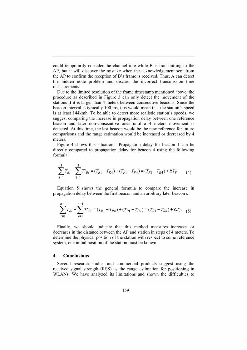
159

could temporarily consider the channel idle while B is transmitting to the AP, but it will discover the mistake when the acknowledgement sent from the AP to confirm the reception of B’s frame is received. Thus, A can detect the hidden node problem and discard the incorrect transmission time measurements.

Due to the limited resolution of the frame timestamp mentioned above, the procedure as described in Figure 3 can only detect the movement of the stations if it is larger than 4 meters between consecutive beacons. Since the beacon interval is typically 100 ms, this would mean that the station’s speed is at least 144kmh. To be able to detect more realistic station’s speeds, we suggest comparing the increase in propagation delay between one reference beacon and later non-consecutive ones until a 4 meters movement is detected. At this time, the last beacon would be the new reference for future comparisons and the range estimation would be increased or decreased by 4 meters.

Figure 4 shows this situation. Propagation delay for beacon 1 can be directly compared to propagation delay for beacon 4 using the following formula:

PRRPPRRi

Bii

Bi TTTTTTTTT ∆+−=−+−=−∑∑==

)()()(' 414141

3

1

3

1 (4)

Equation 5 shows the general formula to compare the increase in

propagation delay between the first beacon and an arbitrary later beacon n:

PRnRPnPRnR

n

iBi

n

iBi TTTTTTTTT ∆+−=−+−=−∑∑

−

=

−

=

)()()(' 111

1

1

1

1 (5)

Finally, we should indicate that this method measures increases or

decreases in the distance between the AP and station in steps of 4 meters. To determine the physical position of the station with respect to some reference system, one initial position of the station must be known.

4 Conclusions Several research studies and commercial products suggest using the

received signal strength (RSS) as the range estimation for positioning in WLANs. We have analyzed its limitations and shown the difficulties to

160

overcome them in practice. We have also looked at a promising alternative, the time of arrival (TOA) range estimation. We found that it could perform better in practice since the impact of the surrounding environment would be less important. But real life experiments are not possible due to the low resolution in the timestamp of the current WLAN chips. Nevertheless, we have suggested a novel approach to measure the variations in range between the AP and the station that does not require synchronized clocks.

References [1] Ekahau, Inc. Ekahau Positioning Engine, September 2003. [2] “An Introduction to Indoor Radio Propagation”, Spread Spectrum

Scene, June 2001, http://www.sss-mag.com/indoor.html. [3] S. Y. Seidel and T. S. Rapport, “914 MHz path loss prediction Model

for Indoor Wireless Communications in Multi-floored buildings,” IEEE Trans. on Antennas & Propagation, Feb. 1992.

[4] Paramvir Bahl and Venkata N. Padmanabhan, “RADAR: An In-Building RF-based User Location and Tracking System”, In Proceedings of IEEE Infocom 2000, 2000.

[5] Kaveh Pahlavan, Xinrong Li, Mika Ylianttila, Ranvir Chana, Matti Latva-aho, “An Overview of Wireless Indoor Geolocation Techniques and Systems”, In Proceedings of IEEE MWCN 2000, pages 1-13, 2000.

[6] Marilynn P. Wylie-Green and S.S. (Peter) Wang, “Robust Range Estimation in the Presence of the Non-Line-of-Sight Error”, In Proceedings of IEEE VTC Fall 2001, volume 1, pages 101-105, 2001.

[7] Anand Balachandran, Geoffrey M. Voelker, Paramvir Bahl, P. Venkat Rangan, “Characterizing User Behavior and Network Performance in A Public Wireless LAN”. In Proceedings of ACM SIGMETRICS 2002, 2002.

[8] D. Mills, “Simple Network Time Protocol (SNTP) Version 4 for IPv4, IPv6 and OSI”, IETF RFC 2030, Oct 1996.

161

OTHER PUBLICATIONS BY THE AUTHOR NOT INCLUDED IN THIS

THESIS • Héctor Velayos and Gunnar Karlsson, “Autonomic networking for

WLANs”, Student Workshop at IEEE Infocom 2005, Miami, Florida, March 2005.

• Héctor Velayos and Gunnar Karlsson, “Analysis of the IEEE 802.11 MAC service time”, 2nd Swedish National Computing Networking Workshop, Karlstad, Sweden, November 2004.

• Héctor Velayos and Gunnar Karlsson, “IP-based distribution system for IEEE 802.11 Wireless LANs”, Radiovetenskap och kommunikation Conference, Stockholm, Sweden, June, 2002.

• J. Manner, A. López, A. Mihailovic, H. Velayos, E. Hepworth and Y. Khouaja, “Evaluation of Mobility and QoS Interaction”, Computer Networks, Vol. 38, Issue 2, Feb. 2002,pp 137-163, Elsevier Science Publisher.

• A. López, J. Manner, A. Mihailovic, H. Velayos, E. Hepworth and Y. Khouaja, “A Study on QoS Provision for IP-based Radio Access Networks”, 2001 Tyrrhenian Int. Workshop on Digital Communications, Taormina, Italy, Sep. 2001.

• T. Robles, A. Kadelka, H. Velayos, A. Lappetelainen, A. Kassler, H. Li, D. Mandato, J. Ojala, B. Wegmann, “QoS support for an all-IP system beyond 3G”, T. Robles, A. Kadelka, H. Velayos, A. Lappetelainen, A. Kassler, H. Li, D. Mandato, J. Ojala and B. Wegmann, IEEE Communication Magazine, Volume: 39 Issue: 8, pp 64-72, Aug. 2001.

• A. López, H. Velayos, J. Manner, N. Villaseñor, “Reservation Based QoS Provision for Mobile Environments”, IEEE 1st Int. Workshop on Services & Applications in the Wireless Public Infrastructure, Evry (Paris), France, 25 - 27 July, 2001.

• G. Neureiter, L. Burness, A. Kassler, P. Khengar, E. Kovacs, D. Mandato, J. Manner, T. Robles, H. Velayos, “The BRAIN quality of service architecture for adaptable services with mobility support”, 11th IEEE PIMRC, London, United Kingdom, Sept. 2000.

Autonomic Wireless Networking

Documents

Transcript of Autonomic Wireless Networking