Automation of T-Spline based 3D High-Fidelity Isogeometric Analysis in Abaqus

Xiang Rena, Jim Lua

a, Xiaodong Wei

b, Yongjie Jessica Zhang

b

aGlobal Engineering and Materials, Inc., Princeton, NJ 08540, USA

bDepartment of Mechanical Engineering, Carnegie Mellon University, Pittsburgh, PA 15213, USA

Abstract: Isogeometric analysis (IGA) has shown its attractive feature recently for integrating a Finite

Element Analysis (FEA) and Computer Aided Design (CAD) into a single unified process. For stress

analysts, it is common practice to convert a spline/NURBS based CAD model to polynomial based finite

element mesh for analysis. However, for complex geometries such as optimized 3D printing objects, it is

known that smooth curved geometry cannot be exactly represented by a discretized finite element mesh. As

a consequence, the simulation results can either be imprecise or costly due to the geometric

misrepresentation or a larger number of degrees of freedom required to achieve the same accuracy. A T-

spline based 3D IGA is developed by CMU to fill the gap. First, a 3D CAD geometry is automatically

converted to a T-spline control mesh, and then it is converted to analysis suitable T-spline elements for a

high fidelity analysis. With unified and higher order T-spline basis functions selected for the geometry

representation, FEA is directly conducted on the smooth CAD geometry without loss of accuracy in

retaining key design details. By taking advantage of the Bézier transformation, the 3D IGA solution module

can be implemented in Abaqus via its user-defined elements (UELs). To accurately pose boundary

conditions for an IGA solution domain from the specified ones at a physical domain, special algorithms are

implemented for mapping the Dirichlet type boundary condition from a physical boundary to the control

points. A suite of numerical examples are selected to demonstrate the accuracy and rate of convergence for

the stress response prediction of complex 3D components.

Keywords: T-Spline, Isogeometric Analysis, Bézier extraction, IGAFA

1. Introduction

The concept of isogeometric analysis (IGA) presented by Hughes (2005) has paved a path towards a close

integration of engineering design and computational analysis. The essential idea of IGA is to apply the

same basis functions for the representation of geometry in Computer-Aided Design (CAD) and the

approximation of field variables in Finite Element Analysis (FEA). Since a single geometry model can be

utilized directly as the analysis model, it can avoid the labor-intensive mesh generation process required for

analysis. In recent years, it has shown its great potential to significantly improve the efficiency of design-

through-analysis cycle. IGA has shown its advantage over standard low-order finite elements in terms of

solution per-degree-of-freedom accuracy via its application in academia problems including fluid

mechanics and turbulence (Evans and Hughes 2013), solid and structure mechanics (Deng et al. 2015),

fluid-structure interaction (Kamensky et al. 2015), phase-field modeling (Borden et al. 2014), contact

mechanics (De Lorenzis et al. 2011 and 2014), and optimization (Kostas et al. 2015). The enhanced

accuracy of IGA is partially due to the higher-order smoothness of the basis functions used. While

significant progress was achieved in the last few years, the biggest challenge is the rapid, (semi-) automatic

construction of geometric models suitable for analysis. Even for a shell structure of a complex geometry, it

is still a time-consuming and challenging process to construct a baseline IGA model, and to ensure the

model has the desired features including good parametrization, sufficient mesh density in the regions of

interest, and, most importantly, analysis suitability. A manually driven partition can be used to push the

limits of existing IGA technology to construct an analysis suitable model but it requires intimate familiarity

with CAD technology. In many cases, a surface representation of a thick structural component is not

sufficient to capture 3D stress distributions at hot spots where geometric discontinuities are present. Design

engineers will have additional burdens when constructing an analysis suitable volumetric T-splines model

for a complex 3D geometry.

A key difficulty for the construction of the volumetric T-splines for a complex geometry is mainly

attributed to the limitation of the current CAD software. Most of the current mainstream CAD software

supports NURBS instead of T-splines. A conversion is required before volumetric T-spline construction,

especially since the CAD design provides only the surface of the geometry. To perform an IGA solid

analysis, the 3D T-spline has to be generated from a surface. In addition, we found that for a complex

geometry, the model reconstruction is usually inevitable regardless of the fact that IGA is designated to

preserve the design geometry. The fundamental reason is that NURBS patches and Boolean operations are

widely applied in the geometry design. As a consequence, the geometry is not warranted analysis suitable.

For the above reasons, it is extremely hard to keep both the absolute designed geometry and the

adaptability of the 3D IGA model. To compromise, a more general approach has to be developed to

reconstruct the geometry based on reparameterization.

In order to reduce the burden on the design iteration for performance optimization, it is imperative to create

a finite element model from CAD geometry directly without data conversion. An isogeometric analysis

toolkit for Abaqus (IGAFA) has been developed in order to reduce the burden on the design iteration for

performance evaluation of advanced structures of complex geometry. In this paper, a T-spline based 3D

IGA toolkit for Abaqus is given first followed by its performance and capability demonstration using

examples for the 3D stress analysis of solid geometries. A 3D CAD geometry is automatically converted to

analysis suitable T-spline representations. By taking advantage of the Bézier extraction, FEA is conducted

by implementing the IGA via Abaqus’ user-defined elements (UELs). To accurately prescribe boundary

conditions for an IGA solution domain, special algorithms are implemented for mapping Dirichlet type

boundary conditions from a physical boundary to the control points. IGA based simulation results are

compared with Abaqus predictions using quadratic solid elements.

1.1 Abaqus-based IGAFA Toolkit

The IGAFA toolkit is developed by us for design and analysis iterations. As shown in Figure 1, the

developed toolkit features 1) automatic T-spline generation from a CAD file; 2) automatic Abaqus input

file generation using the same T-spline based geometric definition; 3) performance of an accurate 3D stress

prediction based on Abaqus UEL elements; and 4) display of 3D stress and strain fields based on physical

Bézier elements using customized Abaqus .odb to guide the design iterations. For each step, we briefly

summarize the key procedures and techniques used.

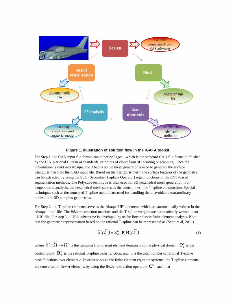
Figure 1. Illustration of solution flow in the IGAFA toolkit

For Step 1, the CAD input file format can either be ‘.iges’, which is the standard CAD file format published

by the U.S. National Bureau of Standards, or points of cloud from 3D printing or scanning. Once the

information is read into Abaqus, the Abaqus native mesh generator is used to generate the surface

triangular mesh for the CAD input file. Based on the triangular mesh, the surface features of the geometry

can be extracted by using the SLO (Secondary Laplace Operator) eigen functions or the CVT-based

segmentation methods. The Polycube technique is then used for 3D hexahedral mesh generation. For

isogeometric analysis, the hexahedral mesh serves as the control mesh for T-spline construction. Special

techniques such as the truncated T-spline method are used for handling the unavoidable extraordinary

nodes in the 3D complex geometries.

For Step 2, the T-spline elements serve as the Abaqus UEL elements which are automatically written in the

Abaqus ‘.inp’ file. The Bézier extraction matrixes and the T-spline weights are automatically written in an

‘.NB’ file. For step 3, a UEL subroutine is developed by us for linear elastic finite element analysis. Note

that the geometric representation based on the rational T-spline can be represented as (Scott et al, 2011)

)~

()~

(x~ e

a

e

a

n

a

e e RP1 (1)

where ee ~

:x~ is the mapping from parent element domain onto the physical domain, e

aP is the

control point, e

aR is the rational T-spline basis function, and ne is the total number of rational T-spline

basis functions over element e. In order to solve the finite element equation systems, the T-spline elements

are converted to Bézier elements by using the Bézier extraction operators e

C , such that

)~

()()~

( eTe PCQ (2a)

)~

()~

( ee BCN (2b)

in which )~

(Q and )~

(B are the Bernstein control point and polynomial basis of the Bézier element,

and )~

(e N is the T-spline polynomial basis. For each UEL element, the stiffness matrix is first integrated

over the parametric domain of the Bézier element by us, and then is assembled into the global stiffness

matrix by Abaqus. Note that the displacements obtained for each UEL element are the ones at the control

points of the T-spline control mesh, and for arbitrary physical locations the displacements, strains, or

stresses can be obtained by interpolation of the control points through rational T-spline basis and their

derivatives. Compared to Abaqus native solver, code optimization has not been conducted in UEL elements

therefore currently the running speed is significantly slower.

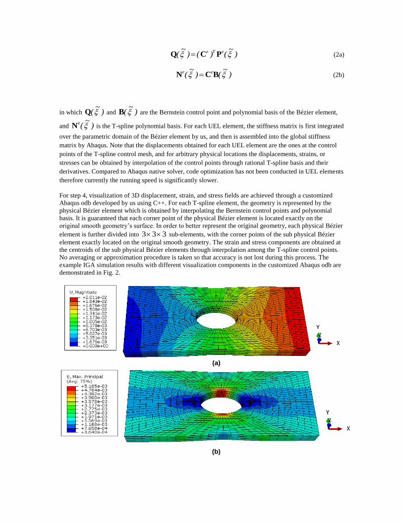
For step 4, visualization of 3D displacement, strain, and stress fields are achieved through a customized

Abaqus odb developed by us using C++. For each T-spline element, the geometry is represented by the

physical Bézier element which is obtained by interpolating the Bernstein control points and polynomial

basis. It is guaranteed that each corner point of the physical Bézier element is located exactly on the

original smooth geometry’s surface. In order to better represent the original geometry, each physical Bézier

element is further divided into 333 sub-elements, with the corner points of the sub physical Bézier

element exactly located on the original smooth geometry. The strain and stress components are obtained at

the centroids of the sub physical Bézier elements through interpolation among the T-spline control points.

No averaging or approximation procedure is taken so that accuracy is not lost during this process. The

example IGA simulation results with different visualization components in the customized Abaqus odb are

demonstrated in Fig. 2.

(a)

(b)

(c)

Figure 2. Visualization of IGA results using customized Abaqus Odb for an example plate-with-hole problem, a) Magnitude of displacement contour, b) Maximum principle strain contour, and c) Mises stress contour. Note that the geometry is visualized by using 128

physical Bézier elements with 3456 physical Bézier sub elements.

1.2 Enhanced solution module for accurate description of IGA boundary conditions

In IGA analysis, the interpolatory property is no longer satisfied everywhere for the control mesh. In other

words, the solution variables at one node can be supported by the ones at the other nodes. As a

consequence, in general situations of the Dirichlet boundary condition such as on the curved surface or with

non-homogenous boundary conditions, the displacements cannot be directly applied at the control points to

represent the real displacements. Special treatment is therefore needed. As such, in order to accurately

apply the Dirichlet type boundary condition and ease the process for users of IGAFA, a preprocessing code

is developed in this regard. The code is written in C++ and can preprocess point-based and surface-based

displacement BCs for 3D geometry. ‘Point-based’ means that the user can specify a displacement BC at

any point of the smooth geometry the 3D T-splines represent, and ‘Surface-based’ means that the user can

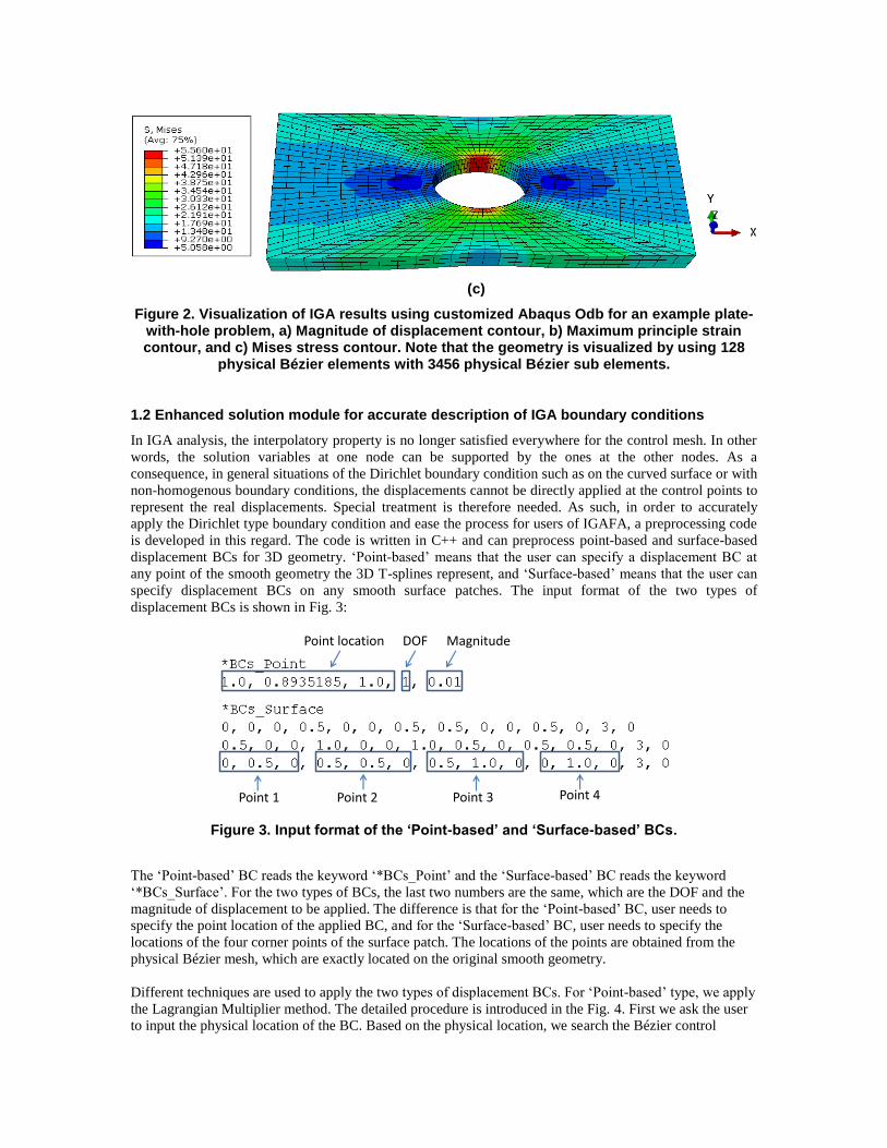
specify displacement BCs on any smooth surface patches. The input format of the two types of

displacement BCs is shown in Fig. 3:

Figure 3. Input format of the ‘Point-based’ and ‘Surface-based’ BCs.

The ‘Point-based’ BC reads the keyword ‘*BCs_Point’ and the ‘Surface-based’ BC reads the keyword

‘*BCs_Surface’. For the two types of BCs, the last two numbers are the same, which are the DOF and the

magnitude of displacement to be applied. The difference is that for the ‘Point-based’ BC, user needs to

specify the point location of the applied BC, and for the ‘Surface-based’ BC, user needs to specify the

locations of the four corner points of the surface patch. The locations of the points are obtained from the

physical Bézier mesh, which are exactly located on the original smooth geometry.

Different techniques are used to apply the two types of displacement BCs. For ‘Point-based’ type, we apply

the Lagrangian Multiplier method. The detailed procedure is introduced in the Fig. 4. First we ask the user

to input the physical location of the BC. Based on the physical location, we search the Bézier control

Point location DOF Magnitude

Point 1Point 2

Point 1 Point 2 Point 3 Point 4

Point location DOF Magnitude

Point 1Point 2

Point 1 Point 2 Point 3 Point 4

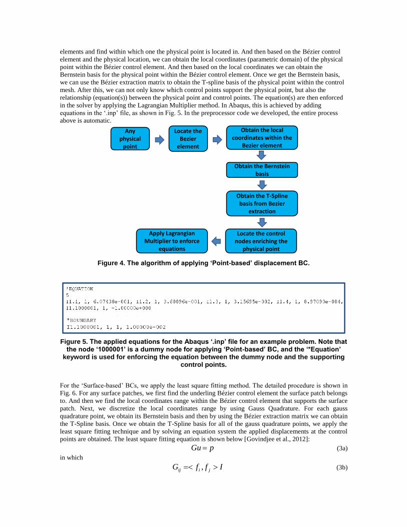
elements and find within which one the physical point is located in. And then based on the Bézier control

element and the physical location, we can obtain the local coordinates (parametric domain) of the physical

point within the Bézier control element. And then based on the local coordinates we can obtain the

Bernstein basis for the physical point within the Bézier control element. Once we get the Bernstein basis,

we can use the Bézier extraction matrix to obtain the T-spline basis of the physical point within the control

mesh. After this, we can not only know which control points support the physical point, but also the

relationship (equation(s)) between the physical point and control points. The equation(s) are then enforced

in the solver by applying the Lagrangian Multiplier method. In Abaqus, this is achieved by adding

equations in the ‘.inp’ file, as shown in Fig. 5. In the preprocessor code we developed, the entire process

above is automatic.

Figure 4. The algorithm of applying ‘Point-based’ displacement BC.

Figure 5. The applied equations for the Abaqus ‘.inp’ file for an example problem. Note that the node ‘1000001’ is a dummy node for applying ‘Point-based’ BC, and the ‘*Equation’

keyword is used for enforcing the equation between the dummy node and the supporting control points.

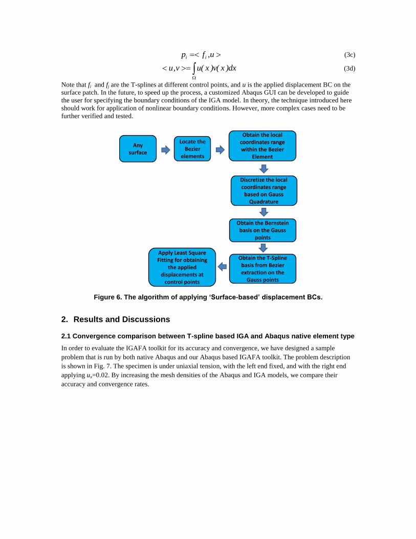
For the ‘Surface-based’ BCs, we apply the least square fitting method. The detailed procedure is shown in

Fig. 6. For any surface patches, we first find the underling Bézier control element the surface patch belongs

to. And then we find the local coordinates range within the Bézier control element that supports the surface

patch. Next, we discretize the local coordinates range by using Gauss Quadrature. For each gauss

quadrature point, we obtain its Bernstein basis and then by using the Bézier extraction matrix we can obtain

the T-Spline basis. Once we obtain the T-Spline basis for all of the gauss quadrature points, we apply the

least square fitting technique and by solving an equation system the applied displacements at the control

points are obtained. The least square fitting equation is shown below [Govindjee et al., 2012]:

pGu (3a)

in which

If,fG jiij (3b)

Any physical

point

Locate the Bezier

element

Obtain the local coordinates within the

Bezier element

Obtain the Bernstein basis

Obtain the T-Spline basis from Bezier

extraction

Locate the control nodes enriching the

physical point

Apply LagrangianMultiplier to enforce

equations

u,fp ii (3c)

dx)x(v)x(uv,u (3d)

Note that fi and fj are the T-splines at different control points, and u is the applied displacement BC on the

surface patch. In the future, to speed up the process, a customized Abaqus GUI can be developed to guide

the user for specifying the boundary conditions of the IGA model. In theory, the technique introduced here

should work for application of nonlinear boundary conditions. However, more complex cases need to be

further verified and tested.

Figure 6. The algorithm of applying ‘Surface-based’ displacement BCs.

2. Results and Discussions

2.1 Convergence comparison between T-spline based IGA and Abaqus native element type

In order to evaluate the IGAFA toolkit for its accuracy and convergence, we have designed a sample

problem that is run by both native Abaqus and our Abaqus based IGAFA toolkit. The problem description

is shown in Fig. 7. The specimen is under uniaxial tension, with the left end fixed, and with the right end

applying ux=0.02. By increasing the mesh densities of the Abaqus and IGA models, we compare their

accuracy and convergence rates.

Any surface

Locate the Bezier

elements

Obtain the local coordinates range within the Bezier

Element

Obtain the Bernstein basis on the Gauss

points

Obtain the T-Spline basis from Bezier extraction on the

Gauss points

Apply Least Square Fitting for obtaining

the applied displacements at

control points

Discretize the local coordinates range

based on Gauss Quadrature

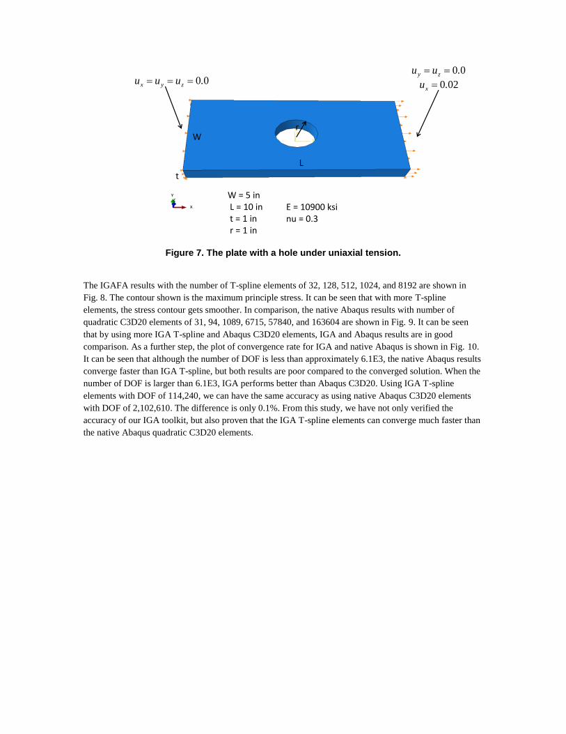
Figure 7. The plate with a hole under uniaxial tension.

The IGAFA results with the number of T-spline elements of 32, 128, 512, 1024, and 8192 are shown in

Fig. 8. The contour shown is the maximum principle stress. It can be seen that with more T-spline

elements, the stress contour gets smoother. In comparison, the native Abaqus results with number of

quadratic C3D20 elements of 31, 94, 1089, 6715, 57840, and 163604 are shown in Fig. 9. It can be seen

that by using more IGA T-spline and Abaqus C3D20 elements, IGA and Abaqus results are in good

comparison. As a further step, the plot of convergence rate for IGA and native Abaqus is shown in Fig. 10.

It can be seen that although the number of DOF is less than approximately 6.1E3, the native Abaqus results

converge faster than IGA T-spline, but both results are poor compared to the converged solution. When the

number of DOF is larger than 6.1E3, IGA performs better than Abaqus C3D20. Using IGA T-spline

elements with DOF of 114,240, we can have the same accuracy as using native Abaqus C3D20 elements

with DOF of 2,102,610. The difference is only 0.1%. From this study, we have not only verified the

accuracy of our IGA toolkit, but also proven that the IGA T-spline elements can converge much faster than

the native Abaqus quadratic C3D20 elements.

L

W

t

r

W = 5 inL = 10 int = 1 inr = 1 in

E = 10900 ksinu = 0.3

00.uuu zyx 00.uu zy

020.ux

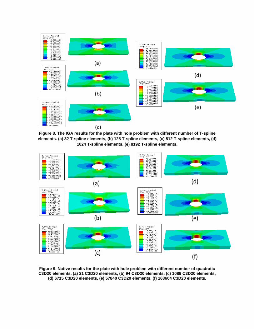
Figure 8. The IGA results for the plate with hole problem with different number of T-spline

elements. (a) 32 T-spline elements, (b) 128 T-spline elements, (c) 512 T-spline elements, (d)

1024 T-spline elements, (e) 8192 T-spline elements.

Figure 9. Native results for the plate with hole problem with different number of quadratic C3D20 elements. (a) 31 C3D20 elements, (b) 94 C3D20 elements, (c) 1089 C3D20 elements,

(d) 6715 C3D20 elements, (e) 57840 C3D20 elements, (f) 163604 C3D20 elements.

(a)

(b)

(c)

(d)

(e)

(a)

(b)

(c)

(d)

(e)

(a)

(b)

(c)

(d)

(e)

(a)

(b)

(c)

(d)

(e)

(a)

(b)

(c)

(d)

(e)

(a)

(b)

(c)

(d)

(e)

(a)

(b)

(c)

(d)

(e)

(a)

(b)

(c)

(d)

(e)

(f)

(a)

(b)

(c)

(d)

(e)

(f)

(a)

(b)

(c)

(d)

(e)

(f)

(a)

(b)

(c)

(d)

(e)

(f)

(a)

(b)

(c)

(d)

(e)

(f)

(a)

(b)

(c)

(d)

(e)

(f)

(a)

(b)

(c)

(d)

(e)

(f)

(a)

(b)

(c)

(d)

(e)

(f)

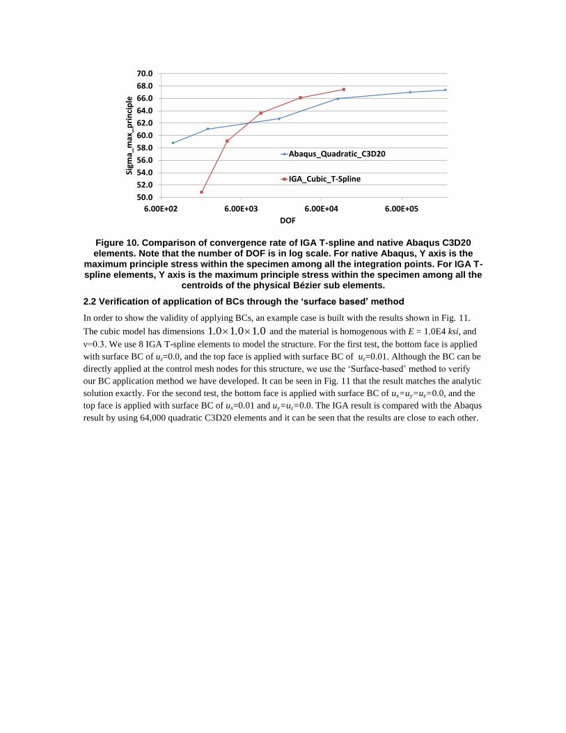
Figure 10. Comparison of convergence rate of IGA T-spline and native Abaqus C3D20 elements. Note that the number of DOF is in log scale. For native Abaqus, Y axis is the

maximum principle stress within the specimen among all the integration points. For IGA T-spline elements, Y axis is the maximum principle stress within the specimen among all the

centroids of the physical Bézier sub elements.

2.2 Verification of application of BCs through the ‘surface based’ method

In order to show the validity of applying BCs, an example case is built with the results shown in Fig. 11.

The cubic model has dimensions 010101 ... and the material is homogenous with E = 1.0E4 ksi, and

ν=0.3. We use 8 IGA T-spline elements to model the structure. For the first test, the bottom face is applied

with surface BC of uz=0.0, and the top face is applied with surface BC of uz=0.01. Although the BC can be

directly applied at the control mesh nodes for this structure, we use the ‘Surface-based’ method to verify

our BC application method we have developed. It can be seen in Fig. 11 that the result matches the analytic

solution exactly. For the second test, the bottom face is applied with surface BC of ux=uy=uz=0.0, and the

top face is applied with surface BC of ux=0.01 and uy=uz=0.0. The IGA result is compared with the Abaqus

result by using 64,000 quadratic C3D20 elements and it can be seen that the results are close to each other.

50.0

52.0

54.0

56.0

58.0

60.0

62.0

64.0

66.0

68.0

70.0

6.00E+02 6.00E+03 6.00E+04 6.00E+05

Sigm

a_m

ax_p

rin

cip

le

DOF

Abaqus_Quadratic_C3D20

IGA_Cubic_T-Spline

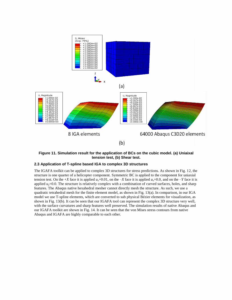
Figure 11. Simulation result for the application of BCs on the cubic model. (a) Uniaixal tension test, (b) Shear test.

2.3 Application of T-spline based IGA to complex 3D structures

The IGAFA toolkit can be applied to complex 3D structures for stress predictions. As shown in Fig. 12, the

structure is one quarter of a helicopter component. Symmetric BC is applied to the component for uniaxial

tension test. On the +X face it is applied ux=0.01, on the –X face it is applied ux=0.0, and on the –Y face it is

applied uy=0.0. The structure is relatively complex with a combination of curved surfaces, holes, and sharp

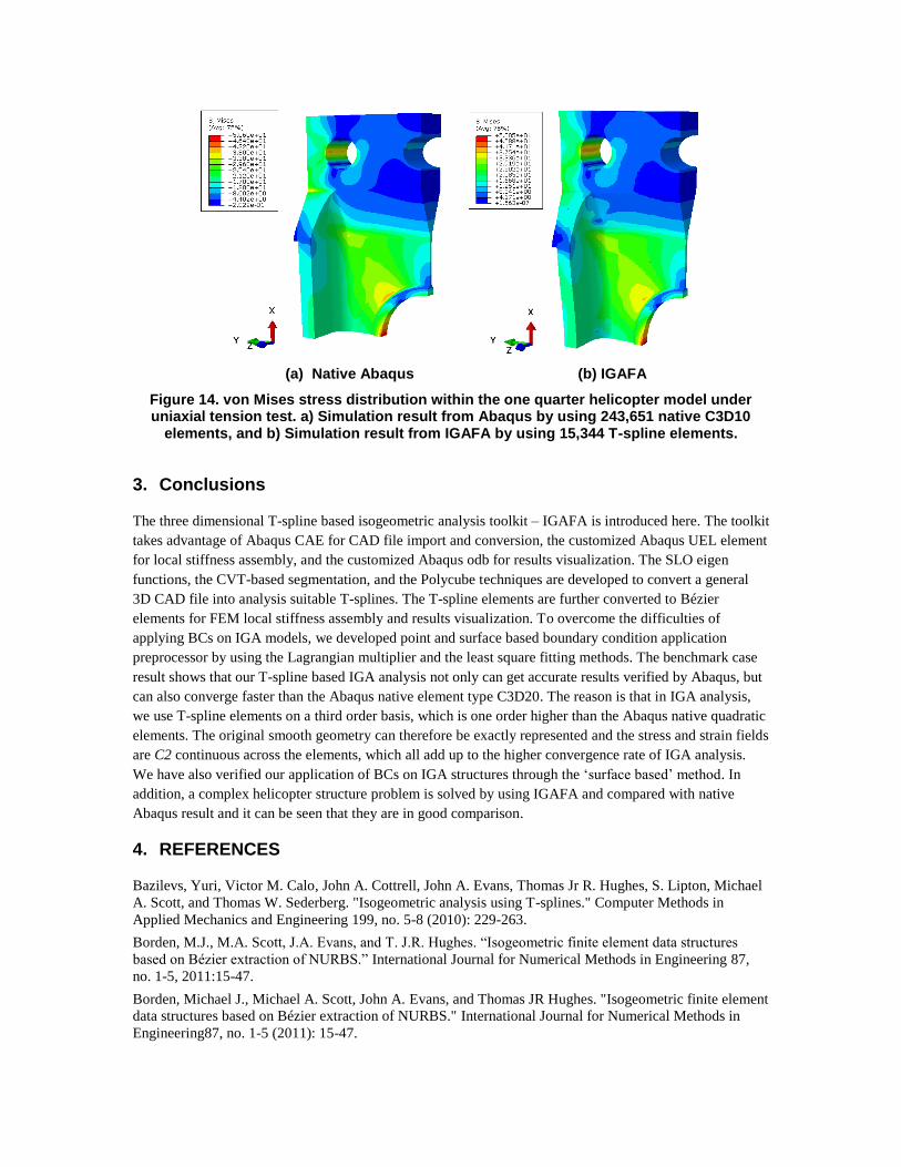
features. The Abaqus native hexahedral mesher cannot directly mesh the structure. As such, we use a

quadratic tetrahedral mesh for the finite element model, as shown in Fig. 13(a). In comparison, in our IGA

model we use T-spline elements, which are converted to sub physical Bézier elements for visualization, as

shown in Fig. 13(b). It can be seen that our IGAFA tool can represent the complex 3D structure very well,

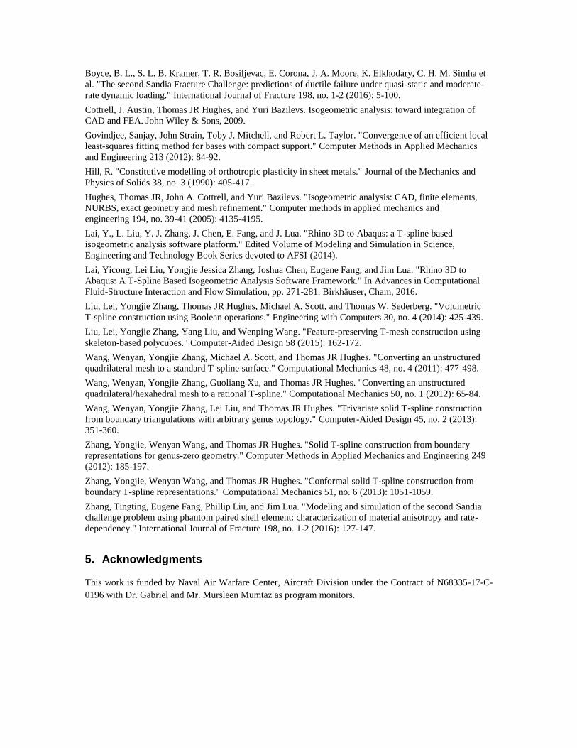
with the surface curvatures and sharp features well preserved. The simulation results of native Abaqus and

our IGAFA toolkit are shown in Fig. 14. It can be seen that the von Mises stress contours from native

Abaqus and IGAFA are highly comparable to each other.

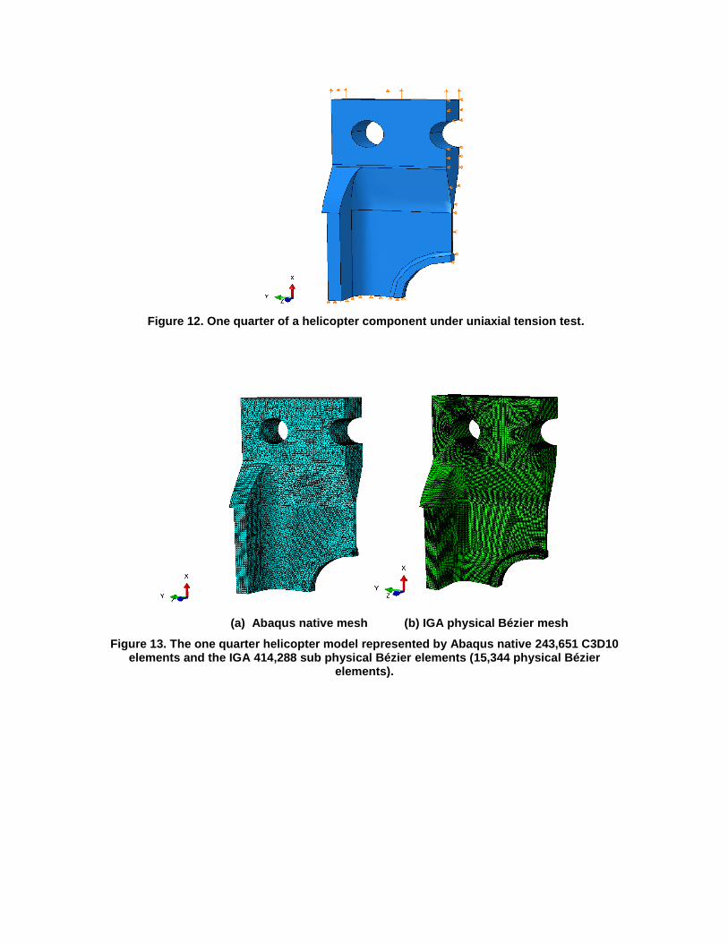
Figure 12. One quarter of a helicopter component under uniaxial tension test.

(a) Abaqus native mesh (b) IGA physical Bézier mesh

Figure 13. The one quarter helicopter model represented by Abaqus native 243,651 C3D10 elements and the IGA 414,288 sub physical Bézier elements (15,344 physical Bézier

elements).

(a) Native Abaqus (b) IGAFA

Figure 14. von Mises stress distribution within the one quarter helicopter model under uniaxial tension test. a) Simulation result from Abaqus by using 243,651 native C3D10

elements, and b) Simulation result from IGAFA by using 15,344 T-spline elements.

3. Conclusions

The three dimensional T-spline based isogeometric analysis toolkit – IGAFA is introduced here. The toolkit

takes advantage of Abaqus CAE for CAD file import and conversion, the customized Abaqus UEL element

for local stiffness assembly, and the customized Abaqus odb for results visualization. The SLO eigen

functions, the CVT-based segmentation, and the Polycube techniques are developed to convert a general

3D CAD file into analysis suitable T-splines. The T-spline elements are further converted to Bézier

elements for FEM local stiffness assembly and results visualization. To overcome the difficulties of

applying BCs on IGA models, we developed point and surface based boundary condition application

preprocessor by using the Lagrangian multiplier and the least square fitting methods. The benchmark case

result shows that our T-spline based IGA analysis not only can get accurate results verified by Abaqus, but

can also converge faster than the Abaqus native element type C3D20. The reason is that in IGA analysis,

we use T-spline elements on a third order basis, which is one order higher than the Abaqus native quadratic

elements. The original smooth geometry can therefore be exactly represented and the stress and strain fields

are C2 continuous across the elements, which all add up to the higher convergence rate of IGA analysis.

We have also verified our application of BCs on IGA structures through the ‘surface based’ method. In

addition, a complex helicopter structure problem is solved by using IGAFA and compared with native

Abaqus result and it can be seen that they are in good comparison.

4. REFERENCES

Bazilevs, Yuri, Victor M. Calo, John A. Cottrell, John A. Evans, Thomas Jr R. Hughes, S. Lipton, Michael

A. Scott, and Thomas W. Sederberg. "Isogeometric analysis using T-splines." Computer Methods in

Applied Mechanics and Engineering 199, no. 5-8 (2010): 229-263.

Borden, M.J., M.A. Scott, J.A. Evans, and T. J.R. Hughes. “Isogeometric finite element data structures

based on Bézier extraction of NURBS.” International Journal for Numerical Methods in Engineering 87,

no. 1-5, 2011:15-47.

Borden, Michael J., Michael A. Scott, John A. Evans, and Thomas JR Hughes. "Isogeometric finite element

data structures based on Bézier extraction of NURBS." International Journal for Numerical Methods in

Engineering87, no. 1-5 (2011): 15-47.

Boyce, B. L., S. L. B. Kramer, T. R. Bosiljevac, E. Corona, J. A. Moore, K. Elkhodary, C. H. M. Simha et

al. "The second Sandia Fracture Challenge: predictions of ductile failure under quasi-static and moderate-

rate dynamic loading." International Journal of Fracture 198, no. 1-2 (2016): 5-100.

Cottrell, J. Austin, Thomas JR Hughes, and Yuri Bazilevs. Isogeometric analysis: toward integration of

CAD and FEA. John Wiley & Sons, 2009.

Govindjee, Sanjay, John Strain, Toby J. Mitchell, and Robert L. Taylor. "Convergence of an efficient local

least-squares fitting method for bases with compact support." Computer Methods in Applied Mechanics

and Engineering 213 (2012): 84-92.

Hill, R. "Constitutive modelling of orthotropic plasticity in sheet metals." Journal of the Mechanics and

Physics of Solids 38, no. 3 (1990): 405-417.

Hughes, Thomas JR, John A. Cottrell, and Yuri Bazilevs. "Isogeometric analysis: CAD, finite elements,

NURBS, exact geometry and mesh refinement." Computer methods in applied mechanics and

engineering 194, no. 39-41 (2005): 4135-4195.

Lai, Y., L. Liu, Y. J. Zhang, J. Chen, E. Fang, and J. Lua. "Rhino 3D to Abaqus: a T-spline based

isogeometric analysis software platform." Edited Volume of Modeling and Simulation in Science,

Engineering and Technology Book Series devoted to AFSI (2014).

Lai, Yicong, Lei Liu, Yongjie Jessica Zhang, Joshua Chen, Eugene Fang, and Jim Lua. "Rhino 3D to

Abaqus: A T-Spline Based Isogeometric Analysis Software Framework." In Advances in Computational

Fluid-Structure Interaction and Flow Simulation, pp. 271-281. Birkhäuser, Cham, 2016.

Liu, Lei, Yongjie Zhang, Thomas JR Hughes, Michael A. Scott, and Thomas W. Sederberg. "Volumetric

T-spline construction using Boolean operations." Engineering with Computers 30, no. 4 (2014): 425-439.

Liu, Lei, Yongjie Zhang, Yang Liu, and Wenping Wang. "Feature-preserving T-mesh construction using

skeleton-based polycubes." Computer-Aided Design 58 (2015): 162-172.

Wang, Wenyan, Yongjie Zhang, Michael A. Scott, and Thomas JR Hughes. "Converting an unstructured

quadrilateral mesh to a standard T-spline surface." Computational Mechanics 48, no. 4 (2011): 477-498.

Wang, Wenyan, Yongjie Zhang, Guoliang Xu, and Thomas JR Hughes. "Converting an unstructured

quadrilateral/hexahedral mesh to a rational T-spline." Computational Mechanics 50, no. 1 (2012): 65-84.

Wang, Wenyan, Yongjie Zhang, Lei Liu, and Thomas JR Hughes. "Trivariate solid T-spline construction

from boundary triangulations with arbitrary genus topology." Computer-Aided Design 45, no. 2 (2013):

351-360.

Zhang, Yongjie, Wenyan Wang, and Thomas JR Hughes. "Solid T-spline construction from boundary

representations for genus-zero geometry." Computer Methods in Applied Mechanics and Engineering 249

(2012): 185-197.

Zhang, Yongjie, Wenyan Wang, and Thomas JR Hughes. "Conformal solid T-spline construction from

boundary T-spline representations." Computational Mechanics 51, no. 6 (2013): 1051-1059.

Zhang, Tingting, Eugene Fang, Phillip Liu, and Jim Lua. "Modeling and simulation of the second Sandia

challenge problem using phantom paired shell element: characterization of material anisotropy and rate-

dependency." International Journal of Fracture 198, no. 1-2 (2016): 127-147.

5. Acknowledgments

This work is funded by Naval Air Warfare Center, Aircraft Division under the Contract of N68335-17-C-

0196 with Dr. Gabriel and Mr. Mursleen Mumtaz as program monitors.