Automatically Georeferencing Textual Documents - ULisboa · Automatically Georeferencing Textual...

Automatically Georeferencing Textual Documents

Fernando José Soares Melo

Thesis to obtain the Master of Science Degree in

Information Systems and Computer Engineering

Supervisor: Prof. Bruno Emanuel da Graça Martins

Examination Committee

Chairperson: Prof. João António Madeiras PereiraSupervisor: Prof. Bruno Emanuel da Graça MartinsMember of the Committee: Prof. José Alberto Rodrigues Pereira Sardinha

June 2015

Abstract

Most documents can be said to be related to some form of geographic context and the

development of computational methods for processing geospatial information, as em-

bedded into natural language descriptions, is a cardinal issue for multiple disciplines. In the con-

text of my M.Sc. thesis, I empirically evaluated automated techniques, based on a hierarchical

representation for the Earth’s surface and leveraging linear classifiers, for assigning geospatial

coordinates of latitude and longitude to previously unseen documents, using only the raw text as

input evidence. Noting that humans may rely on a variety of linguistic constructs to communi-

cate geospatial information, I attempted to measure the extent to which different types (i.e., place

names versus other textual terms) and/or sources of textual content (i.e., curated sources like

Wikipedia, versus general Web contents) can influence the results obtained by automated docu-

ment geocoding methods. The obtained results confirm that general textual terms, besides place

names, can also be highly geo-indicative. Moreover, text from general Web sources can be used

to increase the performance of models based on curated text. The best performing models ob-

tained state-of-the-art results, corresponding to an average prediction error of 88 Kilometers, and

a median error of just 8 Kilometers, in the case of experiments with English documents and when

leveraging Wikipedia contents together with data from hypertext anchors and their surrounding

contexts. In experiments with German, Spanish and Portuguese documents, for which I had

significantly less data taken only from Wikipedia, the same method obtains average prediction

errors of 62, 166 and 105 Kilometers, respectively, and median prediction errors of 5, 13, or 21

Kilometers.

Keywords: Document Geocoding , Natural Language Processing , Hierarchical Text Classifi-

cation , Processing Geospatial Language , Geo-Indicativeness of Textual Contents

i

Resumo

Amaioria dos documentos estao relacionados de alguma forma com um contexto geografico,

sendo o desenvolvimento de metodos computacionais para processar informacao geoespa-

cial, proveniente de discursos de linguagem natural, uma tarefa fundamental para varias areas

cientıficas. No contexto da minha tese de mestrado, avaliei empiricamente, tecnicas automaticas,

baseadas numa representacao hierarquica da superfıcie terrestre, para atribuir coordenadas de

latitude e longitude a documentos, usando apenas o seu texto. Sabendo que os seres humanos

podem utilizar uma variedade de construcoes linguısticas para comunicar informacao geoespa-

cial, eu tentei medir ate que ponto diferentes tipos (i.e., nomes de locais ou outros termos textu-

ais) e/ou diferentes fontes de conteudo textual (i.e., fontes como a Wikipedia ou conteudos gerais

da Web), podem influenciar os resultados obtidos pelos metodos automaticos de geocodificacao.

Os resultados obtidos confirmam que termos textuais comuns, para alem de nomes de locais,

tambem podem ser altamente geo-indicativos. Para alem disso, texto de fontes gerais da Web

pode ser usado para melhorar os resultados obtidos por metodos de geocodificacao automatica

dos documentos da Wikipedia. Obtiveram-se resultados de acordo com o estado-da-arte da

geocoficacao de documentos da Wikipedia, nomeadamente um erro medio de 88 Kilometros

e um erro mediano de 8 Kilometros, para o caso das experiencias da Wikipedia Inglesa, jun-

tamente com o texto de ancoras hipertextuais e o seu contexto envolvente. Relativamente as

experiencias com os documentos da Wikipedia Alema, Espanhola e Portuguesa, para os quais

existem menos dados, retirados apenas da Wikipedia, o mesmo metodo obteve erros medios de

62, 166 e 105 Kilometros, respetivamente, e erros medianos de 5, 13 e 21 Kilometros.

Keywords: Geocodificacao de Documentos , Processamento de Linguagem Natural , Classificacao

Textual Hierarquica , Processamento de Linguagem Geoespacial , Geo-Indicatividade de Conteudos

Textuais

iii

Agradecimentos

Gostaria de agradecer ao professor Bruno Martins, por todo o apoio, disponibilidade, motivacao

lideranca e boa vontade com os quais me orientou durante esta dissertacao de mestrado.

A Fundacao de Ciencias e Tecnologia, pela bolsa de Mestrado no projeto EXPL/EEI-ESS/0427/2013

(KD-LBSN).

Aos meus pais, pelo apoio incondicional demonstrado e por sempre terem acreditado em mim.

A minha namorada Beatriz, pelo seu carinho e amor.

A todos os meus colegas amigos, por tornarem este percurso academico uma experiencia mais

divertida e menos solitaria, ainda que as diretas tenham sido passadas a realizar projetos.

v

Contents

Abstract i

Resumo iii

Agradecimentos v

1 Introduction 1

1.1 Thesis Proposal and Validation Plan . . . . . . . . . . . . . . . . . . . . . . . . . . 2

1.2 Contributions . . . . . . . . . . . . . . . . . . . . . . . . . . . . . . . . . . . . . . . 4

1.3 Document Organization . . . . . . . . . . . . . . . . . . . . . . . . . . . . . . . . . 5

2 Concepts and Related Work 7

2.1 Concepts . . . . . . . . . . . . . . . . . . . . . . . . . . . . . . . . . . . . . . . . . 7

2.1.1 Representing Text for Computational Analysis . . . . . . . . . . . . . . . . . 7

2.1.2 Document Classification . . . . . . . . . . . . . . . . . . . . . . . . . . . . . 10

2.1.3 Geospatial Data Analysis . . . . . . . . . . . . . . . . . . . . . . . . . . . . 13

2.2 Related Work . . . . . . . . . . . . . . . . . . . . . . . . . . . . . . . . . . . . . . . 18

2.2.1 Early Proposals . . . . . . . . . . . . . . . . . . . . . . . . . . . . . . . . . 18

2.2.2 Language Modeling Approaches . . . . . . . . . . . . . . . . . . . . . . . . 21

2.2.3 Modern Combinations of Different Heuristics . . . . . . . . . . . . . . . . . 27

2.2.4 Recent Approaches Based On Discriminative Classification Models . . . . 34

2.3 Summary . . . . . . . . . . . . . . . . . . . . . . . . . . . . . . . . . . . . . . . . . 36

vii

3 Geocoding Textual Documents 39

3.1 The HEALPix Representation for the Earth’s Surface . . . . . . . . . . . . . . . . . 40

3.2 Building Representations . . . . . . . . . . . . . . . . . . . . . . . . . . . . . . . . 42

3.3 Geocoding through Hierarchical Classification for the Textual Documents . . . . . 43

3.4 Summary . . . . . . . . . . . . . . . . . . . . . . . . . . . . . . . . . . . . . . . . . 44

4 Experimental Evaluation 45

4.1 Datasets and Methodology . . . . . . . . . . . . . . . . . . . . . . . . . . . . . . . 45

4.2 Experimental Results . . . . . . . . . . . . . . . . . . . . . . . . . . . . . . . . . . 49

4.3 Summary . . . . . . . . . . . . . . . . . . . . . . . . . . . . . . . . . . . . . . . . . 51

5 Conclusions and Future Work 53

5.1 Conclusions . . . . . . . . . . . . . . . . . . . . . . . . . . . . . . . . . . . . . . . . 53

5.2 Future Work . . . . . . . . . . . . . . . . . . . . . . . . . . . . . . . . . . . . . . . . 54

Bibliography 55

viii

List of Tables

2.1 Comparison between the selection of Location Indicative Words (LIWs) vs using

the full text . . . . . . . . . . . . . . . . . . . . . . . . . . . . . . . . . . . . . . . . 32

2.2 Results obtained using the English Wikipedia dataset . . . . . . . . . . . . . . . . 37

2.3 Results obtained using the German Wikipedia dataset . . . . . . . . . . . . . . . . 37

2.4 Results obtained using the Portuguese Wikipedia dataset . . . . . . . . . . . . . . 37

3.5 Number of regions and approximate area for HEALPix grids of different resolutions. 41

4.6 Statistical characterization for the Wikipedia collections used in our experiments. . 47

4.7 Statistical characterization for the document collections used in our second set of

experiments. . . . . . . . . . . . . . . . . . . . . . . . . . . . . . . . . . . . . . . . 48

4.8 The results obtained for each different language, with different types of textual con-

tents and when using TF-IDF-ICF representations ans Support Vector Machines

as a linear classifier. . . . . . . . . . . . . . . . . . . . . . . . . . . . . . . . . . . . 50

4.9 The results obtained for each different language and for each different linear clas-

sifier, and when using TF-IDF representations. . . . . . . . . . . . . . . . . . . . . 51

4.10 The results obtained for the Twitter datasets using TF-IDF-CF as the document

representation method . . . . . . . . . . . . . . . . . . . . . . . . . . . . . . . . . . 51

4.11 The results obtained with different sources of text, used as a complement or as a

replacement to Wikipedia. . . . . . . . . . . . . . . . . . . . . . . . . . . . . . . . . 52

ix

List of Figures

2.1 A metric ball tree, built from a set of balls in the plane. The middle part illustrates

the binary tree built from the balls on the left, while the right part of the figure

illustrates how space is partitioned with the resulting ball tree. . . . . . . . . . . . . 12

2.2 The hierarchical triangular decomposition of a sphere associated to the HRM ap-

proach. . . . . . . . . . . . . . . . . . . . . . . . . . . . . . . . . . . . . . . . . . . 17

2.3 Illustration for the case when two polygons do not intersect each other. . . . . . . . 20

2.4 Illustration for the case when one polygon is contained in another polygon. . . . . 20

2.5 Illustration for the case when a polygon partially intersects other polygons. . . . . . 20

3.6 Orthographic views associated to the first four levels of the HEALPix sphere tes-

sellation. . . . . . . . . . . . . . . . . . . . . . . . . . . . . . . . . . . . . . . . . . . 40

4.7 Maps with the geographic distribution for the documents in the Wikipedia collections. 46

4.8 Maps with the geographic distribution for the documents in the Twitter collections. . 47

xi

Chapter 1

Introduction

Most documents, from different application domains, can be said to be related to some form

of geographic context. In the recent years, given the increasing volumes of unstructured

information being published online, we have witnessed an increased interest in applying compu-

tational methods to better extract geographic information from heterogeneous and unstructured

data, including textual documents. Geographical Information Retrieval (GIR) has indeed captured

the attention of many different researchers that work in fields related to language processing and

to the retrieval and mining of relevant information from large document collections. Much work

has, for instance, been done on extracting facts and relations about named entities. This includes

studies focused on the extraction and normalization of named places from text, using different

types of natural language processing techniques (DeLozier et al., 2015; Roberts et al., 2010;

Santos et al., 2014; Speriosu & Baldridge, 2013), studies focusing on the extraction of loca-

tive expressions beyond named places (Liu et al., 2014; Wallgrun et al., 2014), studies focusing

on the extraction of qualitative spatial relations between places from natural language descrip-

tions (Khan et al., 2013; Wallgrun et al., 2014), or studies focusing on the extraction of spatial

semantics from natural language descriptions (Kordjamshidi et al., 2011, 2013).

Computational models for understanding geospatial language are a cardinal issue in multiple

disciplines, and they can provide critical support for multiple applications. The task of resolving

individual place references in textual documents has specifically been addressed in several pre-

vious studies, with the aim of supporting subsequent GIR processing tasks, such as document

retrieval or the production of cartographic visualizations from textual documents (Lieberman &

Samet, 2011; Mehler et al., 2006). However, place reference resolution presents several non-

trivial challenges (Amitay et al., 2004), due to the inherent ambiguity of natural language dis-

course (e.g., place names often have other non geographic meanings, different places are often

1

2 CHAPTER 1. INTRODUCTION

referred to by the same name, and the same places are often referred to by different names).

Moreover, there are many vocabulary terms, besides place names, that can frequently appear in

the context of documents related to specific geographic areas. People may, for instance, refer to

vernacular names (e.g., The Alps or Southern Europe) or vague feature types (e.g.,downtown)

which do not have clear administrative borders, and several other types of natural language ex-

pressions can indeed be geo-indicative, even without making explicit use of place names (Adams

& Janowicz, 2012; Adams & McKenzie, 2013). A phrase like dense traffic in the streets as people

rush to their jobs in downtown’s high-rise buildings most likely refers to a large city, while the

phrase walking barefoot in the grass and watching the birds splash in the water is rather asso-

ciated with a natural park. Instead of trying to resolve the individual place references that are

made in textual documents, it may be interesting to instead study methods for assigning entire

documents to geospatial locations (Wing & Baldridge, 2011).

1.1 Thesis Proposal and Validation Plan

In the context of my M.Sc. thesis, relying on recent technical developments in the problem of

document geocoding (Melo & Martins, 2015; Wing & Baldridge, 2014), I propose to evaluate

automated techniques for assigning geospatial coordinates of latitude and longitude to previously

unseen textual documents, using only the raw text of the documents as input evidence. Noting

that humans may rely on a variety of linguistic constructs to communicate geospatial information,

one can perhaps measure to which extent different types (i.e., place names versus other textual

terms) and/or sources of textual content (i.e., curated sources like Wikipedia, versus general

Web contents) can influence the results obtained by automated document geocoding methods.

I also proposed to measure the effectiveness of the proposed document geocoding method on

two Twitter datasets, namely a dataset distributed over the Globe, and a dataset only containing

tweets from the United States.

The general document geocoding methodology, proposed in the context of this thesis, relies

on a hierarchy of linear models (i.e., classifiers based on support vector machines or logistic

regression) together with a discrete hierarchical representation for the Earth’s surface, known in

the literature as the HEALPix approach. The bins at each level of this hierarchical representation,

corresponding to equally-distributed curvilinear and quadrilateral areas of the Earth’s surface, are

initially associated to textual contents (i.e., all the documents from a training set that are known to

refer to particular geospatial coordinates are used and, each area of the Earth’s representation

is associated with the corresponding texts). For each level in the hierarchy, linear classification

models are built using the textual data, relying on a bag-of-words representation, and using

1.1. THESIS PROPOSAL AND VALIDATION PLAN 3

the quadrilateral areas as the target classes. New documents are then assigned to the most

likely quadrilateral area, through the usage of the classifiers inferred from training data. Finally

documents are assigned to their respective coordinates of latitude and longitude, with basis on

the centroid coordinates from the quadrilateral areas.

The main research hypothesis behind this work was that it is possible to achieve state-of-the-art

results in the task of georeferencing textual documents, by using a carefully tuned hierarchical

classifier.

Experiments with different collections of Wikipedia articles, containing documents written in En-

glish, German, Spanish or Portuguese, were performed in order to access the performance of

the proposed geocoding methods. I also attempted to quantify the geoindicativeness of words

that are not place names. To execute this experiment, the words that are considered to be part of

place names were removed through Named Entity Recognition (NER) methods, and the remain-

ing contents were used for training the document geocoding classifiers. The obtained results

show that reasonably good results can still be achieved, thus supporting the idea that general

textual terms can also be highly geo-indicative. The best performing methods leveraged the full

textual contents, obtaining an average prediction error of 82 Kilometers, and a median predic-

tion error of just 8 Kilometers, in the case of documents from the English Wikipedia collection.

For the German, Spanish and Portuguese Wikipedia collections, which are significantly smaller,

the same method obtained an average prediction error of 62, 166 or 105 Kilometers, respectively,

and a median error of 5, 13 or 21 Kilometers. These results are slightly superior to those reported

in previous studies by other authors (Wing & Baldridge, 2011, 2014), although the datasets used

in our experiments may also be slightly different, despite with a similar origin. After removing

place names, the median prediction errors increased to 28, 5, 21 and 37 Kilometers, respectively

in the English, German, Spanish and Portuguese Wikipedia collections. Regarding the Twitter

datasets, the best results for the WORLD dataset correspond to a mean of 1496 and a median of

497 Kilometers, while a mean of 732 and a median of 234 Kilometers were achieved for the US

dataset.

In a second set of experiments, the focus was put on the English language and in the possibility

of including different sources of textual contents to improve the document geocoding task. We

specifically considered different sources as either a complement or as a replacement to the con-

tents from the English Wikipedia, namely: (a) phrases from hypertext anchors, collected from the

Web as a whole and pointing to geo-referenced pages in the English Wikipedia, and (b) phrases

from the hypertext anchors together with other words appearing in the surrounding context. The

obtained results show that text from general Web pages can be used to complement contents

4 CHAPTER 1. INTRODUCTION

from Wikipedia, although the performance drops significantly when using these contents in iso-

lation. The best performing model combined the Wikipedia contents with text from hypertext

anchors and words from the surrounding contexts, achieving a median error of 88 Kilometers

and an average error of 8 Kilometers.

1.2 Contributions

The research made in the context of this thesis has produced the following main contributions:

• State-of-the-art results in the task of document geocoding were achieved, through the use

of Hierarchical Equal Area isoLatitude Pixelization (HEALPix) scheme to divide the Earth’s

surface in subregions, together with a hierarchical classifier based on linear Support Vector

Machines.

• Even after removing place names from the Wikipedia contents, good results are still achieved

in the document geocoding task, which indicates that even common works may be highly

geoindicative.

• Part of the research reported in this dissertation has been accepted for presentation at the

17th EPIA, an international conference on artificial intelligence in Portugal.

The main novel aspects that were introduced in the context of my research are as follows:

• Testing the application of the HEALPix scheme, which produces equal-area discretizations

for the surface of the Earth, in the task of document geocoding;

• Testing the use of a greedy hierarchical procedure, relying on support vector machine clas-

sifiers, in the task of document geocoding;

• Experimented with datasets in multiple languages (i.e., English, Spanish, Portuguese and

German) and from multiple domains (i.e., Wikipedia and Twitter) to evaluate the perfor-

mance of the proposed document geocoding method. Some of these experiments also

involved extended datasets that considered Web anchor text in order to replace or the com-

plement geo-referenced data from Wikipedia.

1.3. DOCUMENT ORGANIZATION 5

1.3 Document Organization

The rest of this document is organized as follows: Chapter 2 describes the fundamental concepts

involved in (i) representing text for computational analysis, (ii)document classification, and (iii)

geospatial data analysis. The chapter ends with the description of studies that have previously

addressed the problem of georeferencing textual contents . Chapter 3 details the contributions of

this thesis, namely (i) the use of the HEALPix scheme in order to discretize the Earth’s surface,

and (ii) the application of hierarchical classification in the document geocoding task. Finally,

Chapters 4 and 5 present the experimental evaluation and the summary of the obtained results,

together with possible paths for future work.

Chapter 2

Concepts and Related Work

This chapter presents the fundamental concepts and the most important related work, in

order to facilitate the understanding of my thesis proposal.

2.1 Concepts

This section presents the main concepts required to fully understand the proposed work, namely

text representations for supporting computational analysis, document classification methods, and

elementary notions from the geographical information sciences.

2.1.1 Representing Text for Computational Analysis

In this section I will describe some of the most common approaches in order to represent text

for computational analysis, namely (i) Bag-of-Words, (ii) The Vector Space Model, and (iii) Other

Approaches For Representing Text

2.1.1.1 Bag-of-Words

Most studies concerned with the analysis of textual contents use the bag-of-words (BoW) rep-

resentation model (Maron & Kuhns, 1960), where the semantics of each document are only

captured through the words that it contains. In order to represent a document using the BoW

method, one is first required to split a document into its constituent words. This process is called

tokenization.

7

8 CHAPTER 2. CONCEPTS AND RELATED WORK

One simple way of tokenizing text is to split a document by the white-space characters (i.e.,

spaces, new lines, and tabs). However, this procedure may result in representations that may

not be the best for several tasks (e.g, this will not capture multi-word expressions such as Los

Angeles). Other tokenization approaches are instead based on n-grams of characters or of

words, considering to some extent the order of the words.

Using a BoW representation, there are several ways to measure the similarity between pairs of

documents. One such way involves using the Jaccard similarity coefficient. Given two documents

A and B, (i.e., given two sets of representative elements such as words or n-grams), we have

that the Jaccard similarity is given by:

Jaccard(A,B) =|A ∩B||A ∪B|

and thus 0 ≤ Jaccard(A,B) ≤ 1 (2.1)

2.1.1.2 The Vector Space Model

A related representation to the BoW method is the Vector Space Model (Salton et al., 1975).

Given a vocabulary T = t1, t2, ..., tn with all the representative elements that exist, in a given

document collection, a document A can be represented as a vector dA =< wt1, wt2, ..., wtn >.

The components wtn represent the weight of element tn for document A. These weights wtn

can be as simple as the frequency with which an element occurs in the document. However, this

simple weighting approach may give high scores for terms that exist in almost every document,

or low scores to rare terms, i.e., the weights are given by looking only at a specific document,

discarding the rest of the documents in a collection, from the computation.

One weighting scheme that attempts to give weights according to the term’s rarity in the corpus

of documents is the term frequency × inverse document frequency procedure (TF-IDF) (Salton

& Buckley, 1988), that calculates the importance of a term t in a document d, contained in the

corpus of documents D.

TF-IDF is perhaps the most popular term weighting scheme, combining the individual frequency

for each element i in the document j (i.e, the Term Frequency component or TF), with the in-

verse frequency of element i in the entire collection of documents (i.e., the Inverse Document

Frequency). The TF-IDF weight of an element i for a document j is given by the following for-

mula:

TF–IDFi,j = log2(1 + TFi,j)× log2

(N

ni

)(2.2)

In the formula, N is the total number of documents in the collection, and ni is the number of

2.1. CONCEPTS 9

documents containing the element i.

In the vector space representation, to find the similarity between pairs of documents, dA and dB ,

one simple approach involves computing the cosine of the angle θ formed between the vectors

dA and dB , given by the formula:

cos(θ) =dA · dB‖dA‖‖dB‖

=dA1dB1 + dA2dB2 + ...+ dAndBn√∑n

i=1 dAi2√∑n

i=1 dBi2

(2.3)

2.1.1.3 Other Approaches For Representing Text

Besides the aforementioned approaches based on a bag-of-words, there are other models that

use a bag-of-concepts (BoC) (Sahlgren & Coster, 2004) approach, in which the intuition is that

that a document can be represented as a distribution over topics, where each topic is a distribu-

tion over a vocabulary.

Latent Dirichlet Allocation (LDA) is a generative probabilistic model that uses the previous notion

of BoC, where each document exhibits multiple topics, and thus can be represented as a distri-

bution of those topics (Blei et al., 2003). Imagine a topic such as Computer Science. This topic

would have high probability for words such as computer, software or program and low probability

for words that are not associated with Computer Science.

A relatively new approach, also corresponding to a BoC model, is the Concise Semantic Analysis

(CSA) method, that was proven to achieve good results in terms of accuracy and computational

efficiency, when compared with popular alternatives (Li et al., 2011).

Besides LDA and CSA, many other approaches have also been introduced in the recent literature

focusing on building document representations. For instance Srivastava et al. (2013) introduced

a deep learning method, namely a type of Deep Boltzmann Machine, that is suitable for extracting

distributed semantic representations from a large unstructured collection of documents, and that

was shown to extract features that outperform other common approaches, such as LDA. Criminisi

et al. (2011) instead proposed approaches based on ensembles of decision trees for learning

effective data representations. In the experiments reported in this dissertation, I have only used

the BoW approach for representing documents, although other alternatives can be considered

for future work.

Besides the aforementioned cosine similarity metric, one other method that can be used to mea-

sure the similarity between pairs of documents, represented as vectors that encode probability

distributions (e.g., over latent topics) is the Kullback–Leibler divergence. The Kullback–Leibler

(KL) divergence measures the distance between two probability distributions, and the smaller the


result, the more similar the distributions are. Given two distributions P and Q, the symmetric

Kullback-Leibler divergence is equal to:

symKL(P,Q) =KL(P ||Q) + KL(Q||P )

2, with KL(X||Y) =

∑i

log

(X(i)

Y(i)

)X(i) (2.4)

In the previous formulas X(i) and Y(i) are the proportions for the topic i in document represen-

tations X and Y, respectively.

2.1.2 Document Classification

Document classification, also known as document categorization, is the task of automatically

assigning classes or categories to textual documents. In this section I will describe some of the

most commonly used classifiers such as: (i) Naive Bayes Classifier, (ii) Discriminative Linear

Classifiers, and (iii) Nearest Neighbor Classifiers

2.1.2.1 Naive Bayes Classifier

Naive Bayes is a simple classifier based on the Bayes theorem (McCallum & Nigam, 1998). The

probability of a document dk, assuming a vocabulary Vdk for the collection of documents, being

generated by a class ci, is computed as:

P(ci|dk) ∝ P(ci)∏

wj∈Vdk

P(wj |ci) (2.5)

Document classification according to the Naive Bayes, method can be made by finding the most

probable class c, for a document dk, expressed in the following equation:

c = argmaxci∈GP(ci)∏

wj∈Vdk

P(wj |ci) (2.6)

In the previous formula, G represents the set of possible classes. The naive Bayes classifier is

called naive because it assumes independence over the features, e.g., in the previous equation

it is assumed that the probability of a word wj appearing in document dk does not depend on the

other words of the document. We know that in a given text, the probability of a word is dependent

on the previous words, e.g. due to syntactic rules. However, despite the naive assumptions,

Naive Bayes Classifiers are known to perform well on several different tasks.

2.1. CONCEPTS 11

2.1.2.2 Discriminative Linear Classifiers

Besides Naive Bayes, we also have that linear discriminative classifiers are commonly used

in document classification applications. Support Vector Machines (SVMs) are one of the most

popular approaches for learning the parameters of linear classifiers from training data. Given n

training instances xi ∈ Rk, i = 1, . . . , n, in two classes yi ∈ {1,−1}, SVMs are trained by solving

the following optimization problem under the constraints yi(w · xi −w0) ≥ 1− ξi, ∀1 ≤ i ≤ n, and

ξi ≥ 0:

arg minw,ξ,w0

{1

2‖w‖2 + C

n∑i=1

ξi

}(2.7)

In the formula, the parameters ξi are non-negative slack variables which measure the degree of

misclassification of the data xi, and C > 0 is a regularization term.

Multi-class classification can also be handled through the procedure above, by first converting

the problem into a set of binary tasks through the one-versus-all scheme (i.e., use a set of binary

classifiers in which each class is fitted against all the other classes, and finally assigning the class

y(x) with the highest value from wy0 +∑ki=1 w

yi xi).

Logistic regression is an alternative linear classification approach, that can also handle multi-

class classification through the one-versus-all scheme. In brief, logistic regression models use

the predictor variables to determine a probability, that is a logistic function of a linear combination

of them (i.e., logistic regression provides estimates of a-posteriori probability for the class mem-

berships, as opposed to SVMs which are more geometrically motivated and focus on finding

a particular optimal separating hyperplane, by maximizing the margin between points closest to

the classification boundary). Logistic regression models can be trained by solving an optimization

problem that is very similar to that of SVMs, instead considering a loss function that is derived

from a probabilistic model:

arg minw,w0

{1

2‖w‖2 + C

n∑i=1

log(1 + e−yi(w·xi−w0))

}(2.8)

Previous studies have argued that SVMs often lead to smaller generalization errors (Caruana &

Niculescu-Mizil, 2006), particularly in the case of high-dimensional datasets, but both types of

models should nonetheless be compared, as their performances change depending on the task.


Figure 2.1: A metric ball tree, built from a set of balls in the plane. The middle part illustrates the binarytree built from the balls on the left, while the right part of the figure illustrates how space is partitioned

with the resulting ball tree.

2.1.2.3 Nearest Neighbor Classifiers

Another frequently used classifier is the k-nn method, that simply consists in finding the docu-

ment’s K nearest neighbours, and then assigning the class with basis on a majority vote. One

efficient way of discovering the top-k most similar documents, involves the use of a geometric

data structure commonly referred to as the metric ball tree (Omohundro, 1989; Uhlmann, 1991).

A ball tree is essentially a binary tree in which every node defines a m-dimensional hypersphere,

containing a subset of the instances to be searched. Each internal node of the tree partitions

the data points into two disjoint sets which are associated with different hyperspheres. While the

hyperspheres themselves may intersect, each point is assigned to one particular hypersphere in

the partition, according to its Euclidean distance towards the hypersphere’s center. Each node in

the tree defines the smallest ball that contains all data points in its subtree. This gives rise to the

useful property that, for a given test instance di, the Euclidean distance to any point in a hyper-

sphere h in the tree is greater than or equal to the Euclidean distance from di to the hypersphere.

Figure 2.1, adapted from a figure given in the technical report by Omohundro (1989), shows an

example of a two-dimensional ball tree.

The search algorithm for answering k nearest neighbor queries can exploit the distance property

of the ball tree, so that if the algorithm is searching the data structure with a test point di, and it has

already seen some point dp that is closest to di among the points that have been encountered so

far, then any subtree whose ball is further from di than dp can be ignored for the rest of the search.

Specifically, the nearest-neighbor algorithm can examine nodes in depth-first order, starting at the

root. During the search, the algorithm maintains a max-first priority queue Q with the k nearest

points encountered so far. At each node h, the algorithm may perform one of following three

operations, before finally returning an updated version of the priority queue:

2.1. CONCEPTS 13

• If the Euclidean distance from the test point di to the current node h is greater than the

furthest point in Q, ignore h and return Q.

• If h is a leaf node, scan through every point enumerated in h and update the nearest-

neighbor queue appropriately. Return the updated queue.

• If h is an internal node, call the algorithm recursively on h’s two children, searching the child

whose center is closer to di first. Return the queue after each of these calls has updated it

in turn.

A metric ball tree is usually built offline and top-down, by recursively splitting the data points into

two sets. Splits are chosen along the single dimension with the greatest spread of points, with

the sets partitioned by the median value of all points along that dimension. A detailed description

of the ball tree data structure is given by Omohundro (1989).

2.1.3 Geospatial Data Analysis

This section explains fundamental concepts from the geographic information sciences, related to

(i) representing locations over the surface of the Earth, (ii) measuring distances, (iii) discretizing

geospatial information and (iv) interpolating geospatial information.

2.1.3.1 Geographic Coordinate Systems and Measuring Distances

Geographic coordinate systems allow us to describe a specific location over the surface of the

Earth, as a set of unambiguous identifiers. One of the most common methods to represent a

specific location is the use of geographic coordinates of latitude and longitude.

The latitude of a geospatial location (i.e., point) is measured as the angle between an horizontal

plane that passes in the equator, and the normal of that geospatial point to an ellipsoid that is

an approximation of the shape of the Earth. The latitude varies between -90°, that represents a

point in the south pole, to 90°, that corresponds to a point in the north pole.

The longitude of a geographic location (i.e., point) is the angle between a reference meridian (e.g.,

the Greenwich Meridian), and the meridian of that specific point (i.e., the plane that separates

the Earth into two equal semi-ellipsoids and passes through the specific point we are refering).

This angle varies between −180°, that correspond to a point in the most extreme West, to 180°,

representing points in the most extreme East.

Given two locations represented by their pair of coordinates of latitude and longitude in degrees


(φ1 , λ1) and (φ2 , λ2), it is not trivial to calculate an accurate distance between these locations,

due to the Earth’s curvature.

One approach that calculates the geospatial distance between two points, by approximating the

Earth’s surface with the surface of a sphere, is the great-circle distance procedure. The first step

of this method is to find the central subtended angle ∆σ, that is the angle formed between the

two lines that link each location to the center of the Earth, given by the formula:

∆σ = arccos(

sin (φ1) sin(φ2) + cos(φ1) cos(φ2)cos(|λ2 − λ1|))

(2.9)

After calculating the central subtended angle in degrees, by using the previous formula, the dis-

tance between the two locations can be estimated by converting this angle to radians, and multi-

plying the angle by the radius of the Earth r, i.e. :

distance = ∆σ × r × π

180(2.10)

As the Earth is not exactly a sphere, its radius varies, being slightly smaller at the poles and

larger at the equator. For this previous method, it is common to choose the mean Earth radius,

that is approximately equal to 6371 km.

Another method to estimate the distance between two coordinates, considering that the Earth can

be approximated to an oblate spheroid (i.e., a rotationally symmetric ellipsoid, whose polar axis is

smaller than the diameter of its equatorial circle) is Vincenty’s inverse method (Vincenty, 1975).

In this method we have that a is the length of the semi-major axis of the ellipsoid (i.e., the radius at

equator); f is the flattening of the ellipsoid; b = (1−f)a is the length of the semi-minor axis of the

ellipsoid (i.e., radius at the poles); U1 = arctan ((1− f) tan(φ1)) and U2 = arctan ((1− f) tan(φ2))

are the reduced latitude (i.e. the latitude on the auxiliary sphere); α is the azimuth at the equator

and σ is the arc length between points on the auxiliary sphere. The first step of this algorithm

is to calculate U1 and U2, and setting λ = λ2 − λ1, followed by iteratively applying the following

equations until λ converges:

sin(σ) =

√(cos(U2) sin(λ))

2+ (cos(U1) sin(U2)− sin(U1) cos(U2) cos(λ))

2 (2.11)

cos(σ) = sin(U1) sin(U2) + cos(U1) cos(U2)cos(λ) (2.12)

2.1. CONCEPTS 15

σ = arctan

(sin(σ)

cos(σ)

)(2.13)

sin(α) =cos(U1) cos(U2) sin(λ)

sin(σ)(2.14)

cos2(α) = 1− sin2(α) (2.15)

cos(2σm) = cos(σ)− 2 sin(U1) sin(U2)

cos2(α)(2.16)

C =f

16cos2(α)[4 + f(4− 3 cos2(α))] (2.17)

λ = L+ (1− C)f sin(α)(σ + C sin(σ)

(cos(2σm) + C cos(σ)(−1 + 2cos2(2σm))

))(2.18)

We iterate λ until it converges to our desired degree of accuracy, and then evaluate the following

equations:

u2 = cos2(α)a2 − b2

b2(2.19)

A = 1 +u2

16384

(4096 + u2

(−768 + u2

(320− 175u2

)))(2.20)

B =u2

1024

(256 + u2

(−128 + u2

(74− 47u2

)))(2.21)

∆σ = B sin(σ)(cos(2σm) + 1

4B(cos(α)(−1 + 2 cos2(2σm))− 1

6B cos(2σm)(−3 + 4 sin2(σ))(−3 + 4 cos2(2σm))))

(2.22)

Finally the distance between the two locations is given by:

distance = bA(σ −∆σ) (2.23)


2.1.3.2 Calculating the Geographic Midpoint of a Point Set

The geographic midpoint is a method of summarizing information from a set of geospatial co-

ordinates, into a single geospatial location, that corresponds to the point that has the minimum

distance to all the original geospatial points. One practical application for the use of a weighted

geographic midpoint is in the domain of georeferencing, when there are several possible loca-

tions, with different probabilities (i.e. different weights), for an object we are trying to locate.

In this subsection, a simple algorithm to find the geographic weighted midpoint between geospa-

tial coordinates of n locations will be presented, following the description originally provided

by (Jeness, 2008).

Given several specific locations represented by their geospatial coordinates of latitude (lat) and

longitude (lon), in degrees, and given a weight that represents the importance of each location

wi, the first step when calculating the geographic midpoint between those locations is to convert

each of the geospatial coordinates from degrees to Cartesian coordinates. One is first required to

convert the coordinates from degrees to radians, which is done by simply multiplying each latitude

and longitude coordinate by π180 . Finally, the Cartesian coordinates are calculated according to:

xi = cos(lati)× cos(loni) yi = cos(lati)× sin(loni) zi = sin(lati) (2.24)

In the previous formula, lati and loni are the latitude and longitude coordinates for each point i,

in radians.

The Cartesian coordinates for the midpoint of the geospatial coordinates that were provided as

input, are simply a weighted average of each geospatial point’s Cartesian coordinates:

x =(x1 × w1) + (x2 × w2) + ...+ (xn × wn)

w1 + w2 + ...+ wn(2.25)

The previous formula shows how to calculate the Cartesian x coordinate for the geospatial mid-

point, and the same logic applies for the y and z coordinates.

The final step is the conversion from Cartesian coordinates to latitude and longitude coordinates

in degrees, which is done by the following formulas:

lat = atan2(z,√x× x+ y × y)× 180 (2.26)

lon = atan2(y, x)× 180 (2.27)

In the previous formulas, atan2 is the arctangent function with two arguments.

2.1. CONCEPTS 17

Figure 2.2: The hierarchical triangular decomposition of a sphere associated to the HRM approach.

2.1.3.3 Hierarchical Tessellations for the Earth’s surface

In geocoding tasks, it is common to discretize the Earth’s surface into several bounded regions.

For instance, the Hierarchical Triangular Mesh (HTM) is a multi-level recursive approach to de-

compose the Earth’s surface into triangles with almost equal shapes and sizes (Szalay et al.,

2005), while the Hierarchical Equal Area isolatitude Pixelization (HEALPix) is instead based on

quadrilateral regions (Gorski et al., 2005).

The HTM offers a convenient approach for indexing data georeferenced to specific points on

the surface of the Earth, having been used in previous studies focusing on document geocod-

ing (Dias et al., 2012). The method starts with an octahedron, as one can see on the left of

Figure 2.2, that has eight spherical triangles, four on the northern hemisphere and four on the

southern hemisphere, resulting from the projection of the edges of the octahedron onto a spher-

ical approximation for the Earth’s surface. These eight spherical triangles are called the level 0

trixels.

Each extra level of decomposition divides each of the trixels into 4 new ones, thus creating smaller

regions. This decomposition is done by adding vertices to the midpoints on each of the previous

level trixels, and then creating great circle arc segments to connect these new vertices in each

trixel, as one can see in the right part of Figure 2.2. The right part of Figure 2.2 shows an

HTM decomposition resulting from dividing the original 8 spherical triangles two times. The total

number of trixels n, for the level of resolution k, is given by n = 8× 4k.

2.1.3.4 Kernel Density Estimation and Interpolating Spatial Data

A fundamental problem in the analysis of data pertaining to georeferenced samples is that

of estimating, with basis on the observed data, the underlying distribution of the samples (i.e.,

the underlying probability density function). Kernel Density Estimation (KDE) can be seen as a

generalization of histogram-based density estimation, which uses a kernel function at each point,


instead of relying on a grid. More formally, the Kernel density estimate for a point (x, y) is given

by the following equation (Carlos et al., 2010):

f(x, y) =1

nh2

n∑i=1

K

(dih

)(2.28)

In the formula, di is the geospatial distance between the occurrence i and the coordinates (x, y),

and n is the total number of occurrences. The bandwidth is given by the parameter h, that controls

the maximum area in which an occurrence has influence. It is very important to choose a correct

h value, because if it is too low, the values will be undersmoothed. The opposite happens when h

is too high, resulting in values that will be oversmoothed, since each point will affect a large area.

Finally, K(.) is the kernel function, that integrates to one and controls how the density diminishes

with the increase of the distance to the target location. A commonly used kernel is the Gaussian

function:

K(u) =1√2πe−u2

2 (2.29)

2.2 Related Work

This section presents the most important previous work that focused in the task of georeferencing

textual documents, describing methods that range from simply discretizing the Earth’s surface

using a grid, estimating a language model for each cell, and finding the most probable cell to

each previously unseen document, to more advanced techniques that create clusters in order to

keep regions with approximately the same sizes, or that rely on discriminative classifiers.

2.2.1 Early Proposals

This section details two seminal works addressing the problem of document geocoding, namely

(i) the GIPSY system described by Woodruff & Plaunt (1994) and (ii) the Web-a-where system

described by Amitay et al. (2004).

Woodruff & Plaunt (1994) developed the Geo-referenced Information Processing System (GIPSY),

as a prototype retrieval service integrating document geocoding functionalities for handling doc-

uments related to the region of California. Document geocoding relied on an auxiliary dataset

containing a subset of US Geological Survey’s Geographic Names Information System (GNIS)

database, that contains geospatial point coordinates of latitude and longitude for over 60,000 ge-

ographic place names in California. Each possible location for a given place name is associated

2.2. RELATED WORK 19

with a probabilistic weight that depends on (1) the geographic terms extracted, (2) the position

within the document and the frequency of these terms, (3) knowledge of the geographic objects

and their attributes on the database, and (4) spatial reasoning about the geographic regions of

the object (e.g. south California).

GIPSY’s document geocoding algorithm can be divided into 3 main steps. Step (i) is a parsing

stage, where the document’s relevant keywords and phrases are extracted. Terms that are re-

lated with geospatial locations in the auxiliary dataset are collected, along with lexical constructs

containing spatial information such as adjacent or neighbouring. In step (ii), in order to obtain the

geographic coordinate data, the system uses spatial datasets that have information such as the

locations of cities, states, names and locations of endangered species, bioregional characteris-

tics of climate regions, etc. The system identifies the spatial locations that are the most similar

with the geographic terms retrieved from step (i). This method also looks for synonym relations

(e.g. the latin and the common name of a specie); membership relations (e.g. when we do not

have geospatial information about a given subspecie but there is information on a hierarchically

superior specie of that subspecie); and geographic reasoning (e.g. south of California).

After extracting all the possible locations for all the place names or phrases in a given document,

the final step overlays polygons in order to estimate approximate locations. Every combination of

place name or phrase, probabilistic weight and geospatial coordinates, is represented as a three

dimensional polygon with base on the plane formed by the x, z axes, and that is elevated upward

on the y axis according to its weight. Each of the polygons for a given document is added one

by one to a skyline that starts empty. When adding a polygon there are three possible scenarios:

(i) the polygon to add does not intersect any of the other polygons, and is mapped to y = 0 (see

Figure 2.3); (ii) the polygon to add is contained in a polygon that has already been added, and its

base is positioned in a higher plane (see Figure 2.4); and (iii) the polygon to add intersects, but

it is not fully contained by one or more polygons, and the polygon to add is split. The portion that

does not intersect any polygon is laid at y = 0, and the portions that intersect polygons are put

on top of the existing polygons they intersect (Figure 2.5).

When all the polygons for a given document are added to the skyline, one can estimate the

geospatial region that best fits a document for example by calculating a weighted average of the

regions that have higher elevation in the skyline generated for the document, or for example by

assuming the document is located in the higher region of the skyline.

In another seminal publication for this area, Amitay et al. (2004) described the Web-a-Where

system for associating a geographic region with a given web page. A hierarchical gazetteer was

used in this work, dividing the world into continents, countries, states (for some countries only)

and cities. The gazetteer contained a total of 40,000 unique places, and a total of 75,000 names


Figure 2.3: Illustration for the case when two polygons do not intersect each other.

Figure 2.4: Illustration for the case when one polygon is contained in another polygon.

for those unique places, which include different spellings and abbreviations. The geocoding

algorithm has 3 main steps, namely (i) spotting, (ii) disambiguation and (iii) focus determination.

On the first step, the goal is to find all the possible locations mentioned in a given web page.

There are some terms that are extracted in this early step and that do not correspond to places,

so a disambiguation step is needed.

There are two possible ambiguities: geo/geo (for example London, England and London, On-

tario), and geo/non-geo (e.g, as London in Jack London, which should be considered part of a

name). In order to disambiguate possible place names, the surrounding words are analyzed. If a

surrounding word is the country, or the state of a place name, a high confidence level is assigned

Figure 2.5: Illustration for the case when a polygon partially intersects other polygons.


to that place name. Each spot that is unresolved is assigned a low confidence and is associated

with the geographical place with the highest population. When there is already a resolved place

name and there are other unresolved occurrences of the same place name, the unresolved place

names are assigned the same geographic region of the resolved place name with a middle value

for the confidence between. Finally, the algorithm attempts to discover the location of unresolved

place names (i.e., those that have a low confidence) through the context. For instance if we

have Hamilton and London , one can infer that the most probable location is Ontario, Canada,

because it is the only place that has both Hamilton and London as descending cities. In this case

the confidence level is increased.

The final step of the geocoding algorithm is to find the focus, i.e. the region that is mostly men-

tioned in the document (e.g. a page mentioning San Francisco (California) and San Diego (Cali-

fornia) has the focus as the taxonomy node California| United States | North America, whereas a

document mentioning Italy, Portugal, Greece and Germany has the focus as the taxonomy node

Europe). The focus algorithm attempts to be as specific as possible. For instance, if the docu-

ment mentions several times Lisbon, and no other cities, nor countries, nor continents, the focus

will be the taxonomy node Lisbon| Portugal | Europe , rather than Portugal | Europe, or Europe

that although correct are not that specific as the first taxonomy node.

The authors used a dataset from the Open Directory Project (ODP) that has almost one million

English pages with a geographic focus. The Web-a-Where system predicted the country that was

the focus of each of these articles with an accuracy of 92%, and a 38% accuracy was measured

for the correct prediction of the city that was the focus of each of these articles.

2.2.2 Language Modeling Approaches

Several previous document geocoding methods are instead based on language modelling ap-

proaches (Dias et al., 2012; Roller et al., 2012; Wing & Baldridge, 2011). A language modelling

approach uses training data in order to estimate the parameters of a model that is able to assign

a probability to a previously unseen sequence of words. A language model is thus a generative

model, defining a probabilistic mechanism for generating language. One of the most popular

language-modeling techniques is the n-gram model, which relies on a Markov assumption in

which the probability of a given word at the ith position, can be approximated to depend only on

the k previous words, instead of depending on all of the previous words, i.e.:

P(wi|w1w2...wi−1) ≈ P(wi|wi−k...wi−1) (2.30)


The simplest n-gram model is based on unigrams, where the k of the previous equation is equal

to 0, and where the probability of a sequence of words is approximated to the multiplication of

the probabilities of each word based on the training data, i.e.:

P (w1w2...wn) ≈∏i

P(wi) =count(wi)

number of tokens(2.31)

A more sophisticated approach, is the bigram language model, where the probability of a word

depends on the previous one, i.e.:

P(wi|w1w2...wi−1) ≈ P(wi|wi−1) =count(wi−1, wi)

count(wi−1)(2.32)

According to the previous equation, one estimates the probability of a word by dividing the total

number of times word i follows word i-1 by the total number of times word i-1 appears. The same

approach can be extended to take into account the last 2 words (the trigram model), the last 3

words (the 4-gram model), etc.

In the previous equation the probability of a word given its previous words is 0 if the event of the

word wi−1 does not follow the word wi, which may be due to the effect of statistical variability

of the training data. Some sort of smoothing, i.e. adding a small probability to unseen events,

is thus required in order to build effective models. One simple method is the Laplace (add-one)

smoothing where, as the name suggests, we simply add one to the numerator of the probability

of a given word, and add the size of the vocabulary V to the denominator (i.e., unseen events

instead of having a probability of 0 will now have a probability of 1V . The probability of observing

the word wi in a bigram model, after Laplace add one smoothing is given by:

P(wi|wi−1) =count(wi−1, wi) + 1

count(wi−1) + V(2.33)

The same smoothing procedure can be generalized to an n-gram model, given by the following

equation:

P(wi|wi−1...wi−n+1) =count(wi−n+1...wi−1wi) + 1

count(wi−n+1...wi−1) + V(2.34)

In the above equation count(wi−n+1...wi−1wi) is the total of times word wi is preceded by the

sequence of the previous n − 1 words (i.e., wi−n+1...wi−2wi−1), and count(wi−n+1...wi−1) is the

number of times the sequence of this previous n− 1 words occurs.

Wing & Baldridge (2011) have for instance investigated the usage of language modelling methods

for automatic document geolocation. The authors started by applying a regular geodesic grid,


with the same latitude and longitude (e.g. 1◦ by 1◦), to divide the Earth’s surface into discrete

rectangular cells. Each of these cells is associated with a cell-document, that is a concatenation

of all the training documents that are located within the cell’s region. The cells that do not contain

any training documents are discarded.

The unsmoothed probability of observing the word j in the cell ci is given by:

P(wj |ci) =

∑dk∈ci

count(wj , dk)∑dk∈ci

∑wl∈V

count(wl, dk)(2.35)

In the previous equation, the unsmoothed probability of observing the word j in the cell ci is

simply calculated by the division of the total number of times word wj appears in all documents

contained in cell ci, by the total of words from the complete vocabulary V that appear in cell ci.

An equivalent distribution P(wj |dk) exists for each test document dk, corresponding to the un-

smoothed probability of observing word wj on document dk:

P(wj |dk) =count(wj , dk)∑

wl∈Vcount(wl, dk)

(2.36)

In the above equation, the probability of an unseen event (i.e., word wj not occurring on document

dk) is 0. If we use Naive Bayes as a classifier to evaluate the probability of document dk having

generated another document that contains the word wj , the probability of the classifier would

be 0, simply because document dk does not contain the word wj , which may occur frequently

in cases where documents are typically short compared to a large vocabulary. The authors

solved the previous issue, by applying a smoothing procedure that reserves a small probability

for unseen events. The smoothed probability for the word j in document dk, contained in D, the

set of all documents, is given by:

P(wj |dk) =

αdk

P(wj |D)1−

∑wl∈dk

P(wl|D) if P(wj |dk) = 0

(1− αdk)P(wj |dk) otherwise

where αdk =|wj ∈ V s.t.count(wj , dk) = 1|∑

wj∈Vcount(wj , dk)

(2.37)

In the previous equations αdk is the probability mass for unseen words, that is equal to the

probability of observing a word only once in document dk, motivated by Good-Turing smoothing.

Analogous procedures were applied to the smoothed cell distributions.

The geolocation algorithm attempts to find the cell-document that is the most similar with each


of the test documents. Three different supervised methods were applied in order to find the most

similar cell for each test document, namely (i) Kullback-Leibler divergence, (ii) Naive Bayes, and

(iii) average cell probability.

The Kullback-Leibler (KL) divergence measures how well a distribution encodes another one,

and the smaller the value, the closer both distributions are. Each cell ci has a distribution that

represents the probabilities of observing each of the words of the vocabulary, and we can thus

find the cell c in the grid G, whose distribution best encodes the test document’s distribution,

given by:

c = argminci∈G∑

wj∈Vdk

P(wj |dk) log

(P(wj |dk)

P(wj |ci)

)(2.38)

In the above equation, wj is a word from the vocabulary Vdk of document dk. In this previous

equation, instead of using the vocabulary for all the existent words, the authors included only

the vocabulary of a document dk, because their experiments have proven that the same result is

achieved in both situations.

As for Naive Bayes it is a simple generative model, based on unigrams, that assumes that the

probability of each word in the document dk does not depend on the previous ones. The cell c

with higher probability is, in this case, given by the equation:

argmaxci∈GP(ci)P(dk|ci)

P(dk)(2.39)

Note that in the previous formula, P(dk) is the same for every cell ci in the grid G, and since the

objective is to find the most probable cell, we can remove the denominator of the equation. The

probability of document dk being located in cell ci is thus calculated by multiplying the probabilities

of a cell ci for each word in document dk:

c = argmaxci∈GP(ci)∏

wj∈Vdk

P(wj |ci)count(wj ,dk) (2.40)

In the previous equation P(wj |ci)count(wj ,dk) is the probability for the word wj in cell ci to the

power of the total number of times word wj appears in the contents of document dk. The authors

calculated the probability of the cell ci (i.e., P(ci)) as being equal to the number of documents in

cell ci, divided by the total number of documents in the corpus.

Finally, the method based on the average cell probability is given by:


c = argmaxci∈G∑

wj∈V dk

count(wj , dk)P(wj |ci)∑

ci∈GP(wj |ci)

(2.41)

In the formula count(wj , dk) is the total number of times word wj appears in the contents of

document dk.

After choosing the most probable cell by one of these methods, the authors assigned to each test

document dk the coordinates of the midpoint of that most probable cell. A prediction error can

finally be calculated using the great-circle distance between the predicted location and the actual

location of the document in the original dataset.

Wing and Baldridge used two different datasets to compare the proposed methods, namely a full

dump of the English version of Wikipedia, from September 2010, and a collection of geotagged

tweets collected by Eisenstein et. al. (2010), from the 48 states of the continental USA. Regard-

ing the Wikipedia articles, they were split 80/10/10 into training, development and testing sets,

whereas in the collection of tweets, the division of training, development and testing sets was al-

ready provided in the data by Eisenstein et. al. (2010). The best results were obtained using the

Kullback-Leibler divergence approach, with Naive Bayes as a close second. For the Wikipedia

dataset, the best results corresponded to a mean error of 221 km and a median error of just 11.8

km. Regarding the Twitter dataset, the authors report on a mean error of 892.0 km and a median

error of 479 km, as the best results that were obtained.

In subsequent work by the same team, Roller et al. (2012) reported on two improvements to the

previously described method.

The first improvement relates to the use of k-d-trees to construct an adaptive grid (Bentley, 1975).

This method deals better with sparsity, producing variable-sized cells that have roughly the same

number of documents in them. In order to find the most probable cell for a given document, the

authors again used the Kullback-Leibler divergence, given that this was the method that had the

most promising results in the previous study.

The second improvement relates to the use of a different measure to choose the location of a cell.

Instead of assigning, to the test document, the coordinates of the midpoint of the most probable

cell, the authors assigned the centroid coordinates of the training documents in that cell.

The authors used three different datasets in this second study, namely the two datasets described

in the previous article, and a third one consisting of 38 million of Tweets located inside North

America . Roller et al. (2012) improved on the results of Wing & Baldridge (2011), reducing the

mean error from 221 km to 181 km and the median error from 11.8 km to 11.0 km, by using

k-d trees instead of uniform grids, and using centroid coordinates instead of the midpoint of the


most probable cell. The mean error was further reduced to 176 km, in an approach combining

uniform grids with k-d trees, that used, as training data, the cell-documents produced by applying

an uniform grid, together with the cell-documents produced by applying a k-d tree. Regarding the

Twitter dataset, the best results were obtained using only the k-d trees, and these correspond to

a mean error of 860 km and a median error of 463 km.

Dias et al. (2012) also evaluated several techniques for automatically geocoding textual doc-

uments (i.e., for assigning textual contents to the corresponding latitude and longitude coordi-

nates), based on language model classifiers, and using only the text of the documents as input

evidence. Experiments were made using georeferenced Wikipedia articles written in English,

Spanish and Portuguese.

These authors used the Hierarchical Triangular Mesh (HTM) method, a multi-level recursive ap-

proach to decompose the Earth’s surface into triangles with almost equal shapes and sizes (Sza-

lay et al., 2005) to partition the geographic space.

In the experiments made by Dias et al., the resolution that was used in the HTM approach varied

from 4 to 10, i.e. from 2048 to 8388608 trixels, that will be associated to language models capable

of capturing the most likely regions for a given document.

The documents were first divided into a training set and test sets. The authors then represented

the documents through either n-grams of characters or of terms (i.e., using 8-grams of characters

or word bi-grams). In what regards the language models based on n-grams of characters, there

are essentially generative models based on the chain rule, smoothed by linear interpolation with

lower order models, and where there is a probability of 1.0 for the sum of all sequences for a

given length. The training documents, associated with the corresponging coordinates, were used

to build a language model for each HTM cell, with the occurrence probabilities for each n-gram.

The authors estimated the distribution P(ci), and also the probability of a document occurring

within the region covered by each specific cell, i.e. P(dk|ci). With these two probabilities, it is

then possible to estimate the probability of a document belonging to a specific cell through Bayes

theorem, i.e. P(ci|dk). This probability, combined with post-processing techniques, allowed the

authors to decide which is the most likely location of a given document.

Every document in the test set is assigned with the most similar(s) region(s) (i.e., the ones with

greater P(ci|dk)). Lastly the latitude and longitude coordinates of each document (in the test set)

can be assigned, for instance with basis on the centroid coordinates of the most similar regions.

Four different post-processing techniques were tested for the assignment of the coordinates to

the documents: (i) the coordinates of the centroid of the most likely region, (ii) the weighted ge-

ographic midpoint of the coordinates of the most likely regions, (iii) a weighted average of the


coordinates of the neighbouring regions of the most likely region and; (iv) the weighted geo-

graphic midpoint of the coordinates of the k − nn most similar training documents, contained in

the most likely region for the document.

The 2nd and 3rd techniques require well calibrated probabilities regarding the possible classes,

while the approach based on language models that was used by the authors is known to produce

extreme probabilities. In order to calibrate the probabilities the authors used a sigmoid function

similar to (σ × score)/(σ − score+ 1), where the σ parameter was empirically adjusted.

The best results were obtained in the English Wikipedia collection, using n-grams of characters,

together with the post-processing method that used the k − nn most similar documents. These

best results correspond to an average error of 265 km, and a median error of 22 km. For the

Spanish and Portuguese collections, the authors obtained an average error of 273 and 278 km,

respectively, and a median error of 45 and 28 km, using the same procedures. The errors re-

ported by the authors correspond to the distance between the original document’s location and

the predicted one, using Vincenty’s geodetic formulae (Vincenty, 1975).

2.2.3 Modern Combinations of Different Heuristics

This section details recent studies that introduced innovative ways of geocoding documents, such

as (i) combining language models from different sources (Laere et al., 2014c); (ii) testing feature

selection methods to improve the prediction of Twitter users’ locations (Bo Han & Baldwin, 2014),

and (iii) leveraging document representations obtained through probabilistic topic models (Adams

& Janowicz, 2012).

We have for instance that Laere et al. (2014c) studied the use of textual information from social

media (i.e. tags on Flickr and words from Twitter messages), in order to aid in the task of georefer-

encing Wikipedia documents. The first step of the proposed algorithm is to find the most probable

region a for a given document D. Instead of using a fixed grid as Wing & Baldridge (2011), the

authors used a k-medoids algorithm, which clusters the training documents into several regions.

Each of these k-clusters contains approximately the same number of documents, which means

that small areas will be created for very dense regions, and larger areas fore more sparse re-

gions. The k-medoids algorithm is similar to k-means, but more robust to outliers (Kaufman &

Rousseeuw, 1987).

After clustering, the authors applied the simple procedure outlined in Algorithm 1 to remove terms

that are not geo-indicative (i.e., that are dispersed all over the world and that are not realated

with specific locations). This algorithm assigns a score to each term from the vocabullary, and

the lower this score is, the more geo-indicative the term is.


Algorithm 1 Geographic spread filtering algorithm (Laere et al., 2014c).

Place a grid over the world map with each cell having sides that correspond to 1 degreelatitude and longitudefor each unique term t in the training data do

for each cell ci,j doDetermine |ti,j |, the number of training documents containing the term tif |ti,j | ≥ 0 then

for each ci′,j′ ∈ {ci−1,j , ci+1,j , ci,j−1, ci,j+1}, i.e. the neighbouring cells of ci,j doDetermine |ti′,j′ |if |ti′,j′ | ≥ 0 and ci,j and ci′,j′ are not already connected then

Connect cells ci,j and ci′,j′end if

end forend if

end forcount = number of remaining connected componentsscore(t) = count

maxi,j |ti,j |end for

Given a clustering Ak and the vocabulary V , it is then possible to estimate language models

for each cluster. The authors estimated separate language models from Wikipedia, Flickr and

Twitter, using the textual contents from Wikipedia articles and from tweets, and the textual tags

assigned to photos in Flickr.

For each test document D, the authors calculated the probabilities for each language model,

for each cluster, to have generated that test document D. The next step was to combine the

probabilities from the different language models for each cluster, in order to find the region a that

has the highest probability of containing the document D.

Naive Bayes was the classifier chosen to find the region a ∈ Ak to where the document D has

the highest probability of belonging to.

The goal is then to find the region a with the highest P(a|D). After moving the equation to log-

space, we have that:

a = argmaxa∈A

(log (P(a)) +

∑t∈VD

log (P(t|a))

)(2.42)

The probability of a region P(a) is calculated as the number of training documents associated

with the region a, divided by the total number of training documents. The probability of a term

t given a region a, i.e., P (t|a), can be calculated by dividing the total number of times the term

t appears in the training documents in a, by the total number of terms in a. However if a term

t does not appear in the training data, its probability would be 0, so some form of smoothing is

required.


The authors applied a Bayesian smoothing procedure with Dirichlet priors:

P(t|a) =Ota + µP(t|V )

Oa + µ,where µ > 0 (2.43)

In the formula, the probability of a term given the vocabulary V in the corpus, i.e., P(t|V ), can

be calculated by dividing the total number of times the term t occurs in the corpus, by the total

number of terms in the corpus. The parameter Ota is the total number of times the term t occurs

in area a, and Oa is the total number of terms that occur in area a, i.e.∑t∈V

Ota.

The final equation to find the most probable area for document D combines the language models

estimated from the different sources S (i.e., from Wikipedia, Twitter and Flickr), and is given by:

a = argmax

( ∑model∈S

λmodel. log (Pmodel(a|D))

)(2.44)

In this last formula the weight of a given model can be controlled by the parameter λmodel. The

authors found that a small weight λTwitter should be assigned, because the Twitter data set

contains noisy information.

Due to memory limitations, the authors only calculated and stored the 100 regions with highest

probabilities for each test document and for each model. The probability of a given document

being in region a is then approximated to:

Pmodel(a|D) =

Pmodel(a|D) if a in top-100

mina′ in top-100Pmodel(a′|D) otherwise

(2.45)

In the previous equation, Pmodel(a|D) is approximated with the minimum of the top-100 most

probable regions for D of that language model, in the cases where Pmodel(a|D) does not belong

to the top-100 most probable areas.

After discovering the area a that best relates with document D, the authors tested three ways

of choosing the coordinates for D namely (i) the medoid, (ii) the Jaccard similarity, and (iii) the

similarity score returned by a well known information retrieval system named Lucene.

The medoid is calculated by searching the document that is closer to all other documents in a

and assigning those coordinates to document D:

ma = argminx∈Train(a)∑

y∈Train(a)

d(x, y) (2.46)


In the previous equation, d(x, y) is the geodesic distance between the coordinates of documents

x and y, i.e. the great circle distance.

The Jaccard similarity is based on searching the training document in the region a that is the

most similar with D, according to this similarity measure, and then assign its coordinates to D.

Finally, the procedure based on Lucene is similar to the previous one, but using Lucene’s internal

similarity measure, which relies on a dot product between TF-IDF vectors.

In their experiments, the authors started by using the Wikipedia dataset from Wing & Baldridge

(2011). However, they detected a number of shortcomings in the previous dataset, such as the

absence of a distinction between articles that describe a specific location and articles whose

location can’t be approximated to a single location, such as countries and rivers. For these

reasons, the authors created a new dataset, where every test document has a precise location

inside the bounding box of the UK. This dataset has a similar size to the one used by Wing &

Baldridge (2011), containing 21 839 test articles and 376 110 training articles.

The authors also created two social media datasets, namely one from Flickr containing 32 million

geolocated and tagged photos, and another one from Twitter containing 16 million georeferenced

tweets, with at least one hashtag.

The baseline results for geocoding Wikipedia documents corresponded to a median error of 4.17

km when using training documents from the same dataset, 2.5 km using the Flickr dataset, and

a median error of 35.81 km for the Twitter dataset. The best results for the combination of Twitter

and Wikipedia documents lowered the median error to 3.69 km, while the best combination be-

tween Wikipedia and Flickr resulted in a median error of just 2.16 km. When combining Wikipedia,

Twitter and Flickr, the best results correspond to a median error of 2.18 km.

Bo Han & Baldwin (2014) also evaluated document geolocation techniques in order to predict

Twitter user locations, based on the text of their tweets. The authors tested the use of numerous

feature selection methods to extract Location indicative Words (LIWs) from the tweets, instead of

using the full text, and the complete vocabulary.

The following datasets were used in this study: (i) a North American dataset by Roller et. al.

(2012) that contains 38 million tweets from 500,000 users from 378 cities (NA); (ii) a worldwide

extraction of tweets created by the authors (from 21 September, 2011 to 29 February, 2012) that

is split into a dataset containing geotagged data only in the English language (WORLD), a dataset

containing English geotagged and non-geotagged data (WORLD + NG), a dataset containing

multilingual geotagged data (WORLD + ML) and a dataset containing English geotagged data

and metadata, namely the users declared locations, real names, descriptions and time zones;

(iii) another worldwide dataset extracted 1 year later than that named WORLD and that is used


only as a test dataset, in order to evaluate the influence of time in the task of predicting Twitter

user locations.

The authors describe several feature selection methods in order to select only words that are

associated with geographical information such as place names, dialectal words, slang or local

references. The information gain ratio was the author’s choice for most of the geolocation predic-

tions, which can be computed as:

IGR(w) =IG(w)

IV(w)

where IG(w) = H(c)−H(c|w)

and where IV(w) = −P(w) log(P(w))− P(w) log(P(w))

(2.47)

In the previous equation, the Information Gain Ratio (IGR) of a word w is the result of the division

between the Information Gain (IG) of that word by the intrinsic entropy (IV) of the word. The

parameter IG(w) represents the decrease in class entropy given by the word w, i.e. the difference

between the entropy of the class, and the entropy of the class given the word w.

The authors used a city-based representation for most of their work, so each class is a city, and

H(c) is the entropy of a given city c. As the final goal is to find which are the top geoindica-

tive words, and since H(c) is equal for all the words, instead of calculating IG(w), we can only

calculate:

H(c|w) = P(w)∑c∈c

P(c|w) log(P (c|w)) + P(w)∑c∈c

P(c|w) log(P (c|w)) (2.48)

In the previous equation P(w) is the probability of finding the word w, whereas P(w) is the prob-

ability of not finding the word w.

Another method used to find LIWs was the Geographic Density (GeoDen), a strategy for selecting

words that occur in dense regions. The GeoDen of a word w is given by:

GeoDen(w) =

∑c∈c′

P(c|w)

|c′|2∑

cj,ck∈c′j 6=k

dist(cj ,ck)

|c′|(|c′|−1)

(2.49)

In the above equation c′ ⊆ c (i.e., c’ is a subset of cities) where word w is used, dist(cj , ck) is the

great-circle distance between cj and ck, and P(c|w) is the probability that a word w has in each

city c ∈ c′. The denominator of the Geographical Density is a product of the square number of

cities where w occurs by the average distance between all cities where w appears.


Table 2.1: Comparison between the selection of Location Indicative Words (LIWs) vs using the full text

Dataset Features Acc Acc@161 Acc@C Median (km)NA Full text 0.171 0.308 0.831 571

IGR 0.260 0.450 0.811 260GeoDen 0.258 0.445 0.791 282

WORLD Full text 0.081 0.200 0.807 886IGR 0.126 0.262 0.684 913GeoDen 0.123 0.266 0.691 842

WORLD +NG

IGR 0.280 0.492 0.878 170

Table 2.1 presents the obtained results using Naive Bayes as a classifier and compares the use of

the full text against using a method to find LIWs such as the IGR, or the Geographic Density. Acc

is the city-level accuracy; Acc@161 is the accuracy within 161km and Acc@C is the country-

level accuracy. One can observe that the addition of 182 million non-geotagged Tweets to a

dataset of 12 million geotagged Tweets (WORLD + NG) clearly improved the obtained results,

demonstrating that non-geotagged Tweets can also be indicative of the user location.

In another previous study, Adams & Janowicz (2012) demonstrated that, besides place names,

some natural language expressions are highly geo-indicative. For instance the words traffic,

income, skyline, government, poverty, or employment probably refer to a large city, whereas

park, hike, rock, flow water, above, or view most likely occur in the context of a description for a

national park.

In order to test if indeed there are words that are good hints to discover the geographic location

associated to a document, the authors relied on experiments with two different data sources,

namely travel blog entries and Wikipedia articles. They also removed all the place names from

every document (i.e., by using Yahoo’s Placemaker1 Web Service to identify the places men-

tioned in the documents), deleted non-English documents and words that belong to an English

standard stop word list, and stemmed the rest of the words.

Adams & Janowicz (2012) divided the Earth’s surface using a geodesic grid with a fixed width and

height, based on decimal degrees. Each training document was then assigned to the cell where

its location is contained. A cell can be seen as the concatenation of all the training documents

contained in its region, similarly to other works that were previously discussed.

After the data pre-processing, Adams & Janowicz (2012) applied the Latent Dirichlet Allocation

(LDA) (Blei et al., 2003) technique to discover T latent topics from the corpus of documents D

and their coordinates P . The result is a |T |-sized vector θd, created for each document, with the

1https://developer.yahoo.com/geo/placemaker/

https://developer.yahoo.com/geo/placemaker/


correspondent probability for each topic. These vectors represent the observed frequency of the

topic at the document’s location. LDA is a generetive model, that assumes documents are the

result from a mixture of topics. Each document has a Dirichlet distribution of the different topics,

and each topic has a Dirichlet distribution of all the possible words. This model assumes that

words are chosen by first selecting a topic, according to the document’s topic distribution, and

then by selecting a word according to the selected topic’s words distribution.

The following step was to estimate the topic vector for each cell, by calculating a weighted aver-

age of the topic values for each document in that given cell. Finally, the centroid point of all the

documents in each cell is associated with the cell’s corresponding topic vector. The authors cal-

culated, for each different topic, a probability surface, by applying the Kernel Density Estimation

(KDE) method, using the cells’ centroid points, and the corresponding cell topic values, except

all the cell points that have the topic value equal to 0.

As previously discussed in this chapter, Kernel Density Estimation (KDE) can be seen as a gen-

eralization of histogram-based density estimation, which uses a kernel function at each point,

instead of relying on a grid. More formally, the Kernel density estimate for a point (x, y) is given

by the following equation (Carlos et al., 2010):

f(x, y) =1

nh2

n∑i=1

K

(dih

)(2.50)

In the formula, di is the geospatial distance between the occurrence i and the coordinates (x, y),

and n is the total number of occurrences. The bandwidth is given by the parameter h, that controls

the maximum area in which an occurrence has influence. It is very important to choose a correct

h value, because if it is too low, the values will be undersmoothed. The opposite happens when h

is too high, resulting in values that will be oversmoothed, since each point will affect a large area.

Finally, K(.) is the kernel function, that integrates to one and controls how the density diminishes

with the increase of the distance to the target location.

Adams & Janowicz (2012) used the Epanechnikov kernel function, given by:

K(u) =3

4(1− u2) with |u| ≤ 1 (2.51)

After having the probability surfaces for each different topic, one can calculate a test document’s

location. The first step is to create the topic vector for the test document, resulting from LDA,

followed by the calculation of a weighted raster overlay via map algebra operations over the

topic probability surfaces, where only the topics that have greater probability than random are

considered, and where the weight for each for each topic is a product of the test document’s topic


weight and its normalized inverse entropy, that measures the topic’s geo-indicativeness.

In order to test this method, sets of 200 held-out documents were used from the travel blog

and Wikipidia datasets. The best results were obtained when using only the top 30 locations

to estimate a document’s coordinates. The top-30 locations for the Wikipedia dataset predicted

75 % of the articles within 505 km and 50 % of them were predicted under 80 km from the real

location. For the travel blog dataset, half of the instances had their location predicted with an

error distance smaller than 1169 km.

2.2.4 Recent Approaches Based On Discriminative Classification Models

In a recent study, Wing & Baldridge (2014) achieved state-of-the-art results on document geocod-

ing by using discriminative classification models. The authors combined a hierarchical division of

the Earth’s surface with the use of logistic regression, relying on a greedy search procedure over

the hierarchy to reduce the time and the storage space required to train and apply the models.

The probability for a logistic regression model of assigning a binary class y ∈ {1,−1} is equal to:

P(y = ±1|x) ≡ 1

1 + e−ywT x(2.52)

In the previous equation x is the data instance and w ∈ Rn is the weight vector, that is chosen in

order to minimize the following equation:

PLR(w) = C

l∑i=1

log(

1 + e−yiwT xi

)+

1

2wTw (2.53)

In the equation above C > 0 is a penalty parameter, and the weights are influenced by the binary

training data {xi, yi}ly=1, xi ∈ Rn, yi ∈ {1,−1}

In order to adapt the previous binary model to a multiclass classification scenario (this is required

to determine which is the most probable cell for a given test document), one can create N binary

models, where a different model is created for each cell, and where the binary classification task

is that of finding the probability of the document belonging to that cell, versus the probability of

not belonging to that cell (i.e., belonging to some other). One can than choose the cell that has

the highest probability for the test document.

The hierarchical division starts with a root node (croot) that covers the entire Earth’s surface, and

from there the authors create a tree of cells, that become smaller from a level to the following.

The authors used an approach originally proposed by Silla & Freitas (2011) in which independent


classifiers are learned in each node of the hierarchy. The probability of a node cj in the hierarchy

is the product of that node multiplied by the probability of all the ancestors of the node, given by

the following recursive equation:

P(croot) = 1.0 P(cj) = P(cj| ↑ cj)P(↑ cj) (2.54)

In the previous equation ↑ cj is cj’s parent node in the hierarchy. In order to avoid computing the

probability of each leaf cell in Equation 2.54, the authors instead used a stratified beam search

where only the b cells with highest probability are kept at each level. A tight beam drastically

reduces the number of classifications required.

Different configurations for the division of the Earth’s surface were tested, based on either a

uniform grid or a k-d tree grid. There are two parameters that influence the grid’s size at each

level. One of these parameters derives from the classifier being used (logistic regression or Naive

Bayes that was employed in this study as a baseline method) and controls the size of the first

level division of the grid. The second parameter is a subdivision factor SF , that defines how the

subdivision is done from one level to the following.

On the uniform grids, each cell is divided into SFxSF subcells, which in practice is not true

because the authors discard every cell that does not contain any training document. For the k-d

trees, if a level 1 has a Bucket size of B, level 2 will have a bucket size of B/SF , level 3 will have

a bucket size of B/SF 2, etc.

Vowpal Wabbit 1 was the implementation of logistic regression classifiers that was chosen, which

leverages an online procedure for model training, together with feature hashing for increased

performance. The authors used 24-bit feature hashing and 12 passes over the data for the subcell

classifiers in hierarchical classification, and 26-bit features and 40 passes over the data for the

remaining classifiers using logistic regression. Feature hashing is a fast way of transforming

features such as words from a Bag of Words representation into a fixed-size vector. Feature

hashing is an alternative to using a dictionary, because it avoids the process of searching through

the text in order to find all different features and then assigning a number to each of them. As the

name implies, a hashing function is used to convert a given feature in a number, and the position

in the feature vector returned by the hashing function holds a frequency count.

Besides the previously described hierarchical procedure using logistic regression (HierLR), the

authors also tested three other classification methods for comparison purposes, namely (i) Naive

Bayes with Dirichlet smoothing (NB); (ii) Naive Bayes with Dirichlet smoothing and with only the

top N features obtained by using the Information Gain Ratio (IGR); and (iii) a logistic regression

1https://github.com/JohnLangford/vowpal_wabbit

https://github.com/JohnLangford/vowpal_wabbit


model applied only to the leaf nodes (FlatLR).

The authors tested their geocoding methods on six distinct datasets:

• TWUS containing 38 million tweets from 450,000 users, where each of them has at least 1

tweet geotagged whitin the bounding box of the United States;

• TWWorld containing 1.4 million users with english geoagged tweets near a city;

• ENWIKI13 an English version of Wikipedia containing 864 thousands of geotagged articles;

• DEWIKI14 a German version of Wikipedia containing 324 thousands of geotagged articles;

• PTWIKI14 a Portuguese version of Wikipedia containing 131 thousands of geotagged arti-

cles;

• COPHIR a dataset from Flickr containing 2.8 millions of geotagged images together with

their correspondent manually-inserted descriptive tags.

The mean, the median and the accuracy at 161 km (acc@161) were used as metrics to evaluate

the different geolocation strategies.

Tables 2.2, 2.3 and 2.4 present the results obtained for the Wikipedia datasets. BK is the bucket

size, SF is the subdivision factor, BM is the beam size and CU is the percentage of the top

geoindicative features that were selected. As one can observe, the document geocoding ap-

proach that uses a hierarchical classifier, together with a k-d tree as a discretization method

achieved the best results for the English and Portuguese versions of Wikipedia, which corre-

spond to an accuracy @ 161 km of 88.9% , a mean error of 168.7 km and a median error of 15.3

km, and an accuracy @ 161 km of 89.5%, a mean error of 186.6 km and a median error of 27.2

km for the Portuguese Wikipedia. In what regards the German version of Wikipedia, the hierar-

chical geocoder that uses k-d trees to discretize the Earth’s surface was still the best geocoder

for the accuracy @ 161 km and for the mean error with 90.2% and 122.5 km respectively. As for

the median, the best geocoder for the German version of Wikipedia was the one that used Naive

Bayes as a classifier, together with k-d trees, achieving a median error of 7.6 km.

2.3 Summary

In this chapter, the most important concepts for understanding the proposed document geocod-

ing method are presented, namely: (i) concepts related to the representation of text for compu-

tational analysis, such as the Vector Space Model where a document is represented as a vector

2.3. SUMMARY 37

Table 2.2: Results obtained using the English Wikipedia dataset

Corpus ENWIKI13Method Parameters A@161 Mean MedNB Uniform 1.5◦ 84.0 326.8 56.3NB k-d BK100 84.5 362.3 21.1IGR Uniform 1.5◦, CU96% 81.4 401.9 58.2IGR k-d BK250, CU98% 80.6 423.9 34.3FlatLR Uniform 7.5◦ 25.5 1347.8 259.4FlatLR k-d BK1500 74.8 253.2 70.0HierLR Uniform 7.5◦, SF3,BM5 86.2 228.3 34.0HierLR k-d BK1500,SF12,BM288.9 168.7 15.3

Table 2.3: Results obtained using the German Wikipedia dataset

Corpus DEWIKI13Method Parameters A@161 Mean MedNB Uniform 1◦ 88.4 257.9 35.0NB k-d BK25 89.3 192.0 7.6IGR Uniform 2◦, CU82% 87.1 312.9 68.2IGR k-d BK50, CU100% 86.0 226.8 10.9FlatLR Uniform 5◦ 55.1 340.4 150.1FlatLR k-d BK350 82.0 193.2 24.5HierLR Uniform 7◦, SF3,BM5 88.5 184.8 30.0HierLR k-d BK3500,SF25,BM590.2 122.5 8.6

Table 2.4: Results obtained using the Portuguese Wikipedia dataset

Corpus PTWIKI13Method Parameters A@161 Mean MedNB Uniform 1◦ 76.6 470.0 48.3NB k-d BK100 77.1 325.0 45.9IGR Uniform 2◦, CU54% 71.3 594.6 89.4IGR k-d BK100,

CU100%71.3 491.9 57.7

FlatLR Uniform 2◦ 88.9 320.0 70.8FlatLR k-d BK25 86.8 320.8 30.0HierLR Uniform 7◦, SF2,BM5 88.6 223.5 64.7HierLR k-d BK250,SF12,BM2 89.5 186.6 27.2


of components, and the TF-IDF weighting heuristic where the weight that a term has on a given

document is a product of its term frequency and its inverse document frequency; (ii) document

classifiers such as Support Vector Machines and Logistic Regression; and (iii) concepts related

to geospatial data analysis.

This chapter also presented an extensive description of the related work on the field of document

geocoding; organizing these previous studies as follows:

• Early Proposals, specifically presenting a document geocoding method for the region of

California (Woodruff & Plaunt, 1994), and a document geocoding method for assigning the

main region described in a given web page (Amitay et al., 2004). Both these approaches

leverage on place names recognized in the text

• Language-modelling approaches consisting of document geocoding approaches that use

a uniform grid, a k-d tree, or a Hierarchical Triangular Mesh to discretize the Earth’s surface,

together with Naive Bayes or the Kullback-Leibler divergence as a classifier to encounter

the most probable region for a given test document (Wing & Baldridge (2011) , Roller et al.

(2012) Dias et al. (2012)).

• Recent Approaches Based on Discriminative Classification Models, specifically pre-

senting the previous study by Wing & Baldridge (2014), which achieved state-of-the-art

results on document geocoding, by using a hierarchical classifier. This is the work that is

the most similiar with the document geociding approach proposed on this thesis, although it

differs on the following aspects: 1) the use of HEALPix to divide the Earth’s surface instead

of a k-d or a uniform grid; 2) the use of TF-IDF or TF-IDF-ICF as document representations

instead of term frequency; and 3) the use of Support Vector Machines as the underlying

classifiers.

Chapter 3

Geocoding Textual Documents

Most text documents, from different application domains, are related to some form of ge-

ographic context. Geographical Information Retrieval (GIR) has recently captured the

attention of many different researchers that work in fields related to language processing and

to the retrieval and mining of relevant information from large document collections. Some previ-

ous works focused on the task of resolving individual place references in textual documents, in

order to support following GIR processing tasks, such as document retrieval or the production

of cartographic visualizations from textual documents (Lieberman & Samet, 2011; Mehler et al.,

2006).

We have, for instance, that the task of resolving individual place references in textual documents

has been addressed in several previous works, with the aim of supporting subsequent GIR pro-

cessing tasks, such as document retrieval or the production of cartographic visualizations from

textual documents (Lieberman & Samet, 2011; Mehler et al., 2006). Instead of trying to resolve

place references made in textual documents, I will instead study methods for assigning entire

documents to correspondent geospatial locations

This chapter presents the geocoding algorithm proposed in the context of my M.Sc. thesis,

detailing the method used to divide the Earth’s surface into a set of regions, the approach taken

in order to transform the text of the documents in representations that the computer may use,

and the hierarchical classification approach.

39

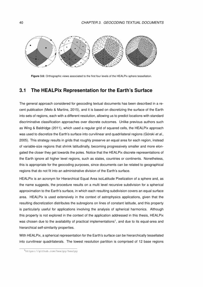
40 CHAPTER 3. GEOCODING TEXTUAL DOCUMENTS

Figure 3.6: Orthographic views associated to the first four levels of the HEALPix sphere tessellation.

3.1 The HEALPix Representation for the Earth’s Surface

The general approach considered for geocoding textual documents has been described in a re-

cent publication (Melo & Martins, 2015), and it is based on discretizing the surface of the Earth

into sets of regions, each with a different resolution, allowing us to predict locations with standard

discriminative classification approaches over discrete outcomes. Unlike previous authors such

as Wing & Baldridge (2011), which used a regular grid of squared cells, the HEALPix approach

was used to discretize the Earth’s surface into curvilinear and quadrilateral regions (Gorski et al.,

2005). This strategy results in grids that roughly preserve an equal area for each region, instead

of variable-size regions that shrink latitudinally, becoming progressively smaller and more elon-

gated the closer they get towards the poles. Notice that the HEALPix discrete representations of

the Earth ignore all higher level regions, such as states, countries or continents. Nonetheless,

this is appropriate for the geocoding purposes, since documents can be related to geographical

regions that do not fit into an administrative division of the Earth’s surface.

HEALPix is an acronym for Hierarchical Equal Area isoLatitude Pixelization of a sphere and, as

the name suggests, the procedure results on a multi level recursive subdivision for a spherical

approximation to the Earth’s surface, in which each resulting subdivision covers an equal surface

area. HEALPix is used extensively in the context of astrophysics applications, given that the

resulting discretization distributes the subregions on lines of constant latitude, and this property

is particularly useful for applications involving the analysis of spherical harmonics. Although

this property is not explored in the context of the application addressed in this thesis, HEALPix

was chosen due to the availability of practical implementations1, and due to its equal-area and

hierarchical self-similarity properties.

With HEALPix, a spherical representation for the Earth’s surface can be hierarchically tessellated

into curvilinear quadrilaterals. The lowest resolution partition is comprised of 12 base regions

1https://github.com/healpy/healpy

https://github.com/healpy/healpy

3.1. THE HEALPIX REPRESENTATION FOR THE EARTH’S SURFACE 41

HEALPix Resolution 4 64 256 1024Total number of regions 192 49,152 786,432 12,582,912Approximate area of each region (Km2) 2,656,625 10,377 649 41

Table 3.5: Number of regions and approximate area for HEALPix grids of different resolutions.

distributed in three rings around the poles and equator, and the resolution of the tessellation

increases by the division of each region into four new ones. Figure 3.6, adapted from the origi-

nal illustration provided in the HEALPix website1, shows from left to right the resolution increase

by three steps from the base level (i.e., a sphere is partitioned, respectively, into 12, 48, 192,

and 768 pixels). The light gray shading shows one of the 8 (4 north and 4 south) identical po-

lar base-resolution regions, while the dark gray shading shows one of the 4 identical equatorial

base-resolution regions. The cells in the resulting mesh are the regions used in our discrete rep-

resentation of the Earth and every curvilinear quadrilateral, at any resolution, is represented by a

single identifier (ID). For each location given by a pair of geospatial coordinates on the surface of

the sphere, there is a discrete ID representing the curvilinear quadrilateral, at a particular resolu-

tion, that contains the corresponding point. An hierarchical binary numbering scheme is normally

adopted for assigning IDs to each curvilinear quadrilateral, where each two bits represent a pixel

number at a given depth (i.e., by shifting off the last two bits one can find the parent pixel number

of a pixel). For more details about the HEALPix procedure, please refer to the paper by Gorski

et al. (2005).

The proposed representation scheme contains a parameter Nside that controls the resolution,

i.e. the number of divisions along the side of a base-resolution region that is needed to reach

a desired high-resolution partition, which naturally will also define the area of the curvilinear

quadrilaterals. In the particular application of document classification, having regions from a

course grained resolution can lead to very rough estimates, but classification accuracy with a

thin-grained resolution can also decrease substantially, due to insufficient data to adjust the model

parameters associated to each bin. In order to address this issue, a hierarchical classification

approach that leverages 4 different representations of different resolutions was used, equaling

the Nside parameter to the values of 22 = 4, 26 = 64, 28 = 256 and 210 = 1024, with 20 = 1

corresponding to a first-level division. Table 3.5 presents the number of regions in each of the

considered resolution levels, where the number of regions n for a resolution Nside is given by n =

12×N2side. Table 3.5 also presents the approximate area, in squared Kilometers, corresponding

to each region.

1http://healpix.jpl.nasa.gov

http://healpix.jpl.nasa.gov


3.2 Building Representations

Besides the issue of building a hierarchy of discrete representations for the surface of the Earth

(i.e., the representations associated to the outcomes, in the context of our classification models),

another important question relates to the choice of how to represent the input instances (i.e.,

the documents to be geocoded). A common representation scheme involves associating each

document to a vector of characteristics in a given vector space, in which the dimensionality cor-

responds to the number of different features. This representation scheme is associated with a

well-known model for processing and representing documents in the area of information retrieval,

commonly referred to as the vector space model (see section 2.1.1 for a more thorough expla-

nation on how to represent text for computational analysis). TF-IDF is perhaps the most popular

term weighting scheme, combining the individual frequency for each element i in the document j

(i.e, the Term Frequency component or TF), with the inverse frequency of element i in the entire

collection of documents (i.e., the Inverse Document Frequency). In this thesis two approaches

for building representations were evaluated, namely (i) the TF-IDF scheme, and (ii) the TF-IDF-

ICF scheme, that complements the TF-IDF method with an additional heuristic corresponding to

the notion of Inverse Class Frequency (ICF), as previously proposed by Lertnattee & Leuviphan

(2012). The idea is to use a simple supervised term weighting scheme (i.e., information on the

membership of training documents to classes is used in the process of building the representa-

tions) that promotes terms that appear in fewer classes (i.e., in fewer regions of the globe) and

demotes terms that appear in many classes. Similar intuitions have already been considered in

previous works related to automated document geocoding (Han et al., 2014; Laere et al., 2014a),

although only for purposes of term selection instead of term weighting. The TF-IDF-ICF weight

of an element i for a document j is given by:

TF–IDF–ICFi,j = log2(1 + TFi,j)× log2

(N

ni

)× log2

(Ncci

)(3.55)

In the formula, N is the total number of documents in the collection, ni is the number of docu-

ments containing the element i, Nc is the total number of classes (i.e., when building the doc-

ument representations leveraging the ICF heuristic, we considered documents to be associated

to classes corresponding to HEALPix regions with a resolution of 64), and ci is the number of

classes associated to documents j′ where TFi,j′ ≥ 0. Through experiments, we found that

both the TF-IDF-ICF and the TF-IDF procedures achieved state-of-the-art results in the task of

geocoding documents.

3.3. GEOCODING THROUGH HIERARCHICAL CLASSIFICATION FOR THE TEXTUAL DOCUMENTS43

3.3 Geocoding through Hierarchical Classification for the Tex-

tual Documents

With the hierarchy of discrete representations given by the HEALPix method, together with the

document representations based on TF-IDF or TF-IDF-ICF, we can use linear classification al-

gorithms to address the document geocoding task. A separate classification model is trained for

each node in the hierarchy of discrete representations, taking all documents whose coordinates

lay within the region corresponding to each node, as the training data for each classifier. When

geocoding a test document, the first step is to apply the root classifier to decide the most likely

region, and then proceed greedily by applying the classifier for each of the most likely nodes,

up to the leafs. After reaching a leaf region from the hierarchical representation, the geospatial

coordinates of latitude and longitude are assigned by taking the centroid coordinates of the leaf

region.

In what follows, we denote by X the input set of documents and by Y our output set of classes

(i.e., geospatial regions). Recall that a classifier is any function which maps objects x ∈ X onto

classes y ∈ Y and, for the purpose of understanding classifiers, it is useful to think about each

x ∈ X as an abstract object which is subject to a set of measurements (i.e., each x takes values

in Rk), which we refer to as features (e.g., the TF-IDF-CF weights for each term in the document).

The experiments reported on this thesis are based on linear classifiers, which make their decision

based on a linear combination of the features, plus a bias term. In the case of binary classification

problems where Y = {+1,−1}, if y(x) is the predicted value for x, if the vector w =< w1, . . . , wk >

corresponds to the weights associated to each of the k features, and if w0 represents the bias

term, then we have that:

y(x) = sign(w0 + w1x1 + . . .+ wkxk) (3.56)

Support Vector Machines (SVMs) are one of the most popular approaches for learning the pa-

rameters of linear classifiers from training data. In the experiments described in this thesis, I

used the SVM and Logistic Regression implementations from scikit-learn1. In the case of logistic

regression classifiers, the probability of class membership is given by:

arg minw,w0

{1

2‖w‖2 + C

n∑i=1

log(1 + e−yi(w·xi−w0))

}(3.57)

1http://scikit-learn.org/

http://scikit-learn.org/


A separate classification model based on one of the previous linear classifiers is trained for each

node in the hierarchy of discrete representations, taking all documents whose coordinates lay

within the region corresponding to each node, as the training data for each classifier. When

geocoding a test document,the root-level classifier is first applied to decide the most likely region,

and then a greedy procedure is followed for each of the most likely nodes, up to the leafs. After

reaching a leaf region from the hierarchical representation, the geospatial coordinates of latitude

and longitude are then assigned to the test document by taking the centroid coordinates of the

leaf region.

3.4 Summary

In this chapter the main ideas behind this thesis are presented, namely the components of a

hierarchical geocoder that assigns geospatial coordinates to a given test document based on

its textual contents, and on the training data. The chapter started by describing HEALPix, a

method for discretizing the Earth’s surface into hierarchical curvilinear quadrilaterals. The chapter

also explained the text representations used for the proposed document geocoding algorithm,

namely TF-IDF and TF-IDF-CF. The chapter ends with a thorough explanation of the hierarchical

document geocoding approach, that was tested with out-of-the-box linear classifiers such as the

implementations of Support Vector Machines and Logistic Regression from scikit-learn.

Chapter 4

Experimental Evaluation

This chapter, describes the experimental methodology used for comparing different varia-

tions of the proposed method, afterwards discussing the obtained results.

4.1 Datasets and Methodology

For the experiments reported here, I used samples with articles from the English, German, Span-

ish, and Portuguese Wikipedias, taken from database dumps produced in 2014. These samples

include a total of 847,783, 307,859, 180,720 and 131,085 articles, respectively in English, Ger-

man, Spanish, and Portuguese, associated to latitude and longitude coordinates. Previous stud-

ies have already shown that Wikipedia articles are a well-suited source of textual contents for

evaluating document geocoding methods (Wing & Baldridge, 2011, 2014).

I processed the Wikipedia collections to extract the raw text from the articles, and for extracting

the geospatial coordinates of latitude and longitude, using manually-defined patterns to capture

some of the multiple templates and formats for expressing coordinates in Wikipedia. Considering

a random order for the articles, about 90% of the geo-referenced articles were used for model

training (i.e., a total of 763,005 articles in English, 277,074 in German, 162,649 in Spanish, and

117,977 in Portuguese), and the other 10% were used for model validation (i.e., a total of 84,778,

30,785, 18,071 and 13,108 articles, respectively in English, German, Spanish and Portuguese).

Table 4.6 presents a brief characterization these datasets, while Figure 4.1 illustrates the geospa-

tial distribution of the locations associated to the documents.

In Table 4.6, the values corresponding to the total number of place references in the collection,

and the number of place references in each document, were obtained from the application of

45

46 CHAPTER 4. EXPERIMENTAL EVALUATION

Figure 4.7: Maps with the geographic distribution for the documents in the Wikipedia collections.

a Named Entity Recognition (NER) system over the texts, in order to extract location names. I

have specifically used Stanford NER, together with models trained for each language. In what

regards the geospatial distributions of documents, notice that some regions (e.g, North America

or Europe) are considerable more dense in terms of document associations than others (e.g,

Africa). We can also see that in the Portuguese collection there is a higher concentration of

articles in Europe and in South America (i.e., in Brazil), and that in the Spanish collection there

is a higher concentration of articles in Europe and in latin South-American countries. Moreover,

oceans and other large masses of water are scarce in associations to Wikipedia documents. This

implies that the number of classes that has to be considered by this model is much smaller than

the theoretical number of classes given in Table 3.5. In the English dataset, there are a total of

286,966 bins containing associations to documents at resolution of 1024, and a total of 82,574,

15,065, and 190 bins, respectively at resolutions 256, 64, and 4. These numbers are even smaller

in the other collections, e.g. with just 98,139, 100,335 and 72,109 bins containing associations

to documents in a resolution of 1024, respectively in the case of the German, Spanish and

Portuguese collections.

In order to evaluate the effectiveness of the proposed document geocoding approach, I also

used a dataset from Roller et al. (2012) named Twitter-US that contains 38 million tweets 450

thousand users. In the dataset, a document is the result of the concatenation of all tweets by

4.1. DATASETS AND METHODOLOGY 47

EN Wikipedia Train Test DE Wikipedia Train TestDocuments 763,005 84,778 Documents 277,074 30,785Terms 279,886,310 30,936,884 Terms 132,464,428 14,614,460Place References 11,326,826 1,289,530 Place References 4,023,883 446,339Avg. Terms/Doc. 366.821 364.916 Avg. Terms/Doc. 478.083 474.727St.Dev. Terms/Doc. 767.537 739.657 St.Dev. Terms/Doc. 869.365 815.676Avg. Places/Doc. 14.845 15.211 Avg. Places/Doc. 14.523 14.499St.Dev. Places/Doc. 26.080 25.460 St.Dev. Places/Doc. 27.751 26.632

ES Wikipedia Train Test PT Wikipedia Train TestDocuments 162,649 18,071 Documents 117,976 13,108Terms 57,067,617 6,304,936 Terms 21,424,167 2,397,775Place References 1,431,185 173,642 Place References 479,602 52,958Avg. Terms/Doc. 350.864 348.898 Avg. Terms/Doc. 181.598 182.925St.Dev. Terms/Doc. 880.160 893.109 St.Dev. Terms/Doc. 606.659 587.515Avg. Places/Doc. 8.779 9.609 Avg. Places/Doc. 4.065 4.040St.Dev. Places/Doc. 19.166 21.173 St.Dev. Places/Doc. 8.688 8.072

Table 4.6: Statistical characterization for the Wikipedia collections used in our experiments.

Figure 4.8: Maps with the geographic distribution for the documents in the Twitter collections.

a given user, that has at least one geotagged tweet with specific coordinates of latitude and

longitude. The earliest geotagged tweet from a given user is considered the user’s location. In

this dataset, tweets outside a bounding box covering the United States were discarded, together

with potential spammers or robots (given the number of tweets, followers and followees). I used

another dataset from Twitter, named Twitter-World, collected from Han & Baldwin (2012), that

is similar from the previous, but instead has geotagged tweets that cover the Earth’s surface

and it only has geotagged tweets. The authors also removed non-english tweets, tweets that

are not near a city, short tweets and non-aphabetic tweets. The resulting dataset has 12 million

tweets from 1.4 million users. Figure 4.1 shows the geospatial distribution for Twitter-US and

Twitter-World datasets.

In a second set of experiments, the performance of the document geocoding method was evalu-

ated over different sources of text, taking these sources either as a complement or as a replace-

ment to the geo-referenced contents from the English Wikipedia, using Support Vector Machines


Corpus size Vocabulary Terms per document(words) size Average St.dev

Wikipedia 311,670,977 7,217,371 367.631 764.793Anchor text 46,375,708 1,772,058 54.702 389.399Wikipedia + anchor text 324,378,152 7,243,824 382.619 896.209Anchor text + context 236,263,101 4,112,659 278.683 5418.008Wikipedia + anchors + context 514,503,489 9,183,943 606.881 5679.983

Table 4.7: Statistical characterization for the document collections used in our second set ofexperiments.

as the linear model for the hierarchical classifiers, and TF-IDF-ICF method to build the document

representations. Two different sources of text were considered in these experiments:

• Phrases from hypertext anchors, collected from the Web as a whole and pointing to geo-

referenced pages in the English Wikipedia. I specifically made use of a dataset released

by Google1, obtained by iterating over this search engine’s Web index. I used the text of

the hypertext anchors either as a replacement to the Wikipedia contents (i.e., the training

instances instead consisted of the title of the Wikipedia pages plus the concatenation of all

hypertext anchors), or as a complement to the contents in Wikipedia (i.e., concatenating

the hypertext anchors to the Wikipedia documents).

• Phrases from the hypertext anchors together with other words appearing in the surrounding

context, as made available in an expanded version of Google’s original dataset (Singh et al.,

2012). In this expanded version, the text of the hypertext anchors is made available together

with the surrounding words (i.e., words either at the left or the right of the anchor text). I

again used these contents either a complement or as a replacement to the geo-referenced

contents from the English Wikipedia.

One of the reasons behind experimenting with the usage of these datasets to help geocod-

ing Wikipedia documents is due to the fact the anchor text associated to links towards

geo-referenced Wikipedia pages, together with the words from the surrounding context,

can offer compact descriptions for the main contents of these pages. We therefore believe

that these textual contents can providing some valuable extra information, that can perhaps

improve the results of the document geocoding method.

Table 4.7 presents a statistical characterization of the different datasets used in this second set

of experiments.

1https://code.google.com/p/wiki-links/

https://code.google.com/p/wiki-links/

4.2. EXPERIMENTAL RESULTS 49

I also evaluated the performance of the proposed document geocoding method after, (i) removing

all the terms that were considered as being part of a place name, with the use of Stanford NER

models for each language (dataset Without Place Names), (ii) storing the set of all titles for a

given Wikipedia collection and then removing all the occurences of a Wikipedia title from each

document (dataset Without Wiki Titles).

4.2 Experimental Results

Table 4.8 presents the obtained results for geo-referenced documents from the English Wikipedia

using , (i) the full content of its pages, (ii) the textual contents without place references, and (iii) the

textual contents after removing all matches towards titles of geo-referenced Wikipedia pages. In

these experiments I used TF-IDF-CF as a document representation approach, together with SVM

classifiers. The prediction errors shown in Table 4.8 correspond to the distance in Kilometers,

computed through Vincenty’s geodetic formulae, from the predicted locations to the true locations

given in the gold standard. The accuracy values correspond to the relative number of times that

we could assign documents to the correct bin (i.e., the bin where the document’s true geospatial

coordinates of latitude and longitude are contained), for each level of hierarchical classification.

The table also presents upper and lower bounds for the average and median errors, according

to a 95% confidence interval and as measured through a t-test (for the average) or through a

sampling procedure (for the median).

As expected, the results from Table 4.8 show that classifiers leveraging the full-contents achieve

better results, with a best prediction accuracy of over 0.95 in the task of finding the correct bin

with the 1st level classifier, in the case of the English collection, while assigning documents to the

correct geospatial coordinates had an average error of 87 Kilometers, and a median error of 8

Kilometers, also in the case of the English collection. Although better results are achieved when

using the entire contents of the Wikipedia articles, it should nontheless be noticed that even when

using models trained with contents where the place names have been removed or where all the

titles were removed from the text of the documents, interesting results were achieved, given the

circumstances, thus suggesting that other terms besides place names can also be geo-indicative

The obtained results also attest to the general effectiveness of the proposed document geocoding

method, as we have measured slightly inferior errors than those reported in the previous studies

by Wing & Baldridge (2011, 2014) in section 2.2. It should nonetheless be noted that the datasets

used in our experiments may be slightly different from those used by Wing and Baldridge, de-

spite their similar origin. The hyper-parameters used in the classification approach (i.e., the C


Classifier accuracy Errors in terms of distance (Km)Full Wikipedia 1st 2nd 3rd 4th Average MedianEnglish 0.967 0.786 0.547 0.272 86.616 (±4.517) 8.308 [5.134 - 14.413]German 0.974 0.844 0.670 0.423 62.046 (±6.075) 4.628 [3.432 - 7.150]Spanish 0.951 0.722 0.446 0.167 184.385 (±18.223) 12.546 [8.392 - 22.691]Portuguese 0.954 0.670 0.344 0.112 108.505 (±10.249) 20.606 [13.105 - 32.020]

Classifier accuracy Errors in terms of distance (Km)Without Place Names 1st 2nd 3rd 4th Average MedianEnglish 0.867 0.548 0.343 0.177 448.892 (±11.160) 28.015 [12.359 - 68.293]German 0.949 0.787 0.609 0.376 150.271 (±10.579) 5.417 [3.759 - 10.422]Spanish 0.889 0.588 0.349 0.133 357.856 (±21.949) 21.302 [11.460 - 44.815]Portuguese 0.912 0.523 0.261 0.094 240.727 (±16.773) 37.365 [20.623 - 65.839]

Classifier accuracy Errors in terms of distance (Km)Without Wiki Titles 1st 2nd 3rd 4th Average MedianEnglish 0.873 0.553 0.346 0.167 422.966 (±11.572) 26.871 [12.459 - 63.683]German 0.940 0.731 0.530 0.305 161.063 (±10.071) 8.221 [4.734 - 18.681]Spanish 0.881 0.542 0.305 0.113 372.164 (±22.627) 29.672 [15.214 - 65.492]Portuguese 0.906 0.537 0.249 0.079 274.119 (±20.653) 34.300 [21.0350 - 56.665]

Table 4.8: The results obtained for each different language, with different types of textual contents andwhen using TF-IDF-ICF representations ans Support Vector Machines as a linear classifier.

regularization term for the SVM classifiers) were also kept at the default values and, for future

work, one could use automated procedures to tune the parameters of the classifiers (Claesen

et al., 2014), and also to experiment with different hierarchical organizations (i.e., with different

numbers of levels and/or with different resolutions in the hierarchical classification procedure).

Table 4.9 presents results for a document geocoding method that represents documents using

the TF-IDF method, together with classifiers based on SVMs or logistic regression. The English

version of Wikipedia achieved a mean of 83 Km and a median of 9 Km for the approach that uses

SVMs as linear classifiers. The German, Spanish and Portuguese versions of Wikipedia achieved

means of 63, 166, and 105 Km, and medians of 5, 13, and 22 Km, when using SVMs as linear

classifiers. Inferior results were achieved when using logistic regression as linear classifier. As

one can observe similar results were achieved both using TF-IDF or TF-IDF-ICF. The first method

usually achieves slightly better mean results, whereas TF-IDF-ICF usually achieves slightly better

median results.

Table 4.10 describes the results for the Twitter datasets, namely a mean of 1496 km and a median

of 497 km for the Twitter-World dataset, and a mean of 732 km, and a median of 234 km for the

Twitter-US dataset. This results show that the proposed geocoding method can also be used

to geolocate tweets, since we achieved better mean error and similar median error results than

Wing & Baldridge (2014), for the Twitter World dataset, that report a mean error of 1670 Km and

a median error of 490 Km.

Table 4.11 presents the obtained results when using external datasets as a complement or an

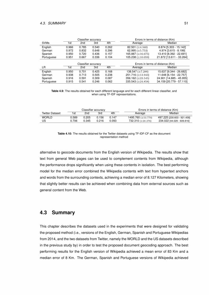
4.3. SUMMARY 51

Classifier accuracy Errors in terms of distance (Km)SVMs 1st 2nd 3rd 4th Average MedianEnglish 0.966 0.785 0.540 0.262 82.501 (±4.340) 8.874 [5.303 - 15.142]German 0.972 0.832 0.648 0.396 62.995 (±5.753) 4.974 [3.615 - 8.199]Spanish 0.950 0.720 0.436 0.157 165.887 (±16.675) 13.410 [8.392 - 22.691]Portuguese 0.951 0.667 0.336 0.104 105.238 (±10.059) 21.872 [13.611 - 33.264]

Classifier accuracy Errors in terms of distance (Km)LR 1st 2nd 3rd 4th Average MedianEnglish 0.950 0.701 0.425 0.168 138.547 (±7.288) 15.637 [9.344 - 26.682]German 0.938 0.713 0.505 0.238 251.716 (±13.943) 11.648 [6.154 - 22.757]Spanish 0.916 0.591 0.309 0.087 356.162 (±23.545) 24.901 [14.885 - 45.955]Portuguese 0.915 0.541 0.246 0.062 335.543 (±24.858) 34.159 [20.779 - 57.110]

Table 4.9: The results obtained for each different language and for each different linear classifier, andwhen using TF-IDF representations.

Classifier accuracy Errors in terms of distance (Km)Twitter Dataset 1st 2nd 3rd 4th Average MedianWORLD 0.589 0.205 0.156 0.147 1495.760 (±53.770) 497.225 [230.603 - 921.458]US 0.706 0.345 0.216 0.093 732.310 (±20.276) 234.022 [44.029 - 609.816]

Table 4.10: The results obtained for the Twitter datasets using TF-IDF-CF as the documentrepresentation method

alternative to geocode documents from the English version of Wikipedia. The results show that

text from general Web pages can be used to complement contents from Wikipedia, although

the performance drops significantly when using these contents in isolation. The best performing

model for the median error combined the Wikipedia contents with text from hypertext anchors

and words from the surrounding contexts, achieving a median error of 8.127 Kilometers, showing

that slightly better results can be achieved when combining data from external sources such as

general content from the Web.

4.3 Summary

This chapter describes the datasets used in the experiments that were designed for validating

the proposed method (i.e., versions of the English, German, Spanish and Portuguese Wikipedias

from 2014, and the two datasets from Twitter, namely the WORLD and the US datasets described

in the previous study by) in order to test the proposed document geocoding approach. The best

performing results for the English version of Wikipedia achieved a mean error of 83 Km and a

median error of 8 Km. The German, Spanish and Portuguese versions of Wikipedia achieved


Classifier accuracy Errors in terms of distance (Km)1st 2nd 3rd 4th Average Median

Wikipedia text 0.967 0.786 0.547 0.272 86.616 (±4.517) 8.308 [5.134 - 14.413]Anchors 00.00 00.00 00.00 00.00 273.355 (±10.13) 44.587 [2.315 - 22.315]Wikipedia + anchors 0.967 0.786 0.548 0.273 85.808 (±4.490) 8.299 [4.998 - 14.348]Anchors + context 0.915 0.644 0.387 0.182 246.102 (±8.084) 18.583 [9.983 - 33.107]Wikipedia + anchors + context 0.967 0.790 0.551 0.274 88.068 (±4.657) 8.178 [5.024 - 14.055]

Table 4.11: The results obtained with different sources of text, used as a complement or as areplacement to Wikipedia.

mean errors of 62, 166 and 105 Km and median errors of 5, 13, and 21 Km respectively, demon-

strating that state-of-the-art results were achieved with this document geocoding algorithm. It

was also shown that even common words may be highly geoindicative, in an experiment where

the place names occurring in the contents of each Wikipedia version were first removed using

Stanford NER. The results, after removing place names, for the English version of Wikipedia were

a mean error of 449 Km and a median error of 28 Km, and mean errors of 150, 358, and 241 Km,

and median errors of 5, 21, and 37 Km respectively for the German, Spanish and Portuguese

Wikipedias. I also tested the use of external datasets to complement the geocoding of Wikipedia

documents. The best results were achieved with a Google dataset that contains anchors that re-

fer to the English Wikipedia pages, together with surrounding context, and correspond to a mean

error of 88 Km, and a median error of 8 Km. The best results for the WORLD Twitter dataset were

a mean of 1496 Km and a median error of 497 km, and a mean error of 732 km, while a median

error of 234 km for the US Twitter dataset, results that are comparable with the ones reported by

(Wing & Baldridge, 2014).

Chapter 5

Conclusions and Future Work

This chapter summarizes the main conclusions from my research work, and presents some

suggestions of possible future work on the mining of geospatial information from textual

documents.

5.1 Conclusions

Through this study, I empirically evaluated automated methods for document geo-referencing

over textual contents of different types (i.e., place names versus other textual terms) and/or from

different sources (i.e., curated sources like Wikipedia, versus general Web contents). The re-

sults confirm that the automatic identification of the geospatial location of a document, based

only on its text, can be performed with high accuracy by using out-of-the-box implementations of

well-known supervised classification methods, and leveraging a discrete binned representation

of the Earth’s surface based on the HEALPix scheme. The results also show that reasonably

good results can still be achieved when place names are removed from the textual contents, thus

supporting the idea that general textual terms can be highly geo-indicative. When comparing the

performance of models trained with contents from different sources, we saw that text from gen-

eral Web pages (i.e., text from hypertext anchors point to geo-referenced Wikipedia documents,

and words from the contexts surrounding these hypertext links) can be used to complement con-

tents from Wikipedia, although the performance drops significantly when using these contents in

isolation. One of the best performing approaches leveraged SVMs classification models and text

representations based on TF-IDF-ICF achieving a median error of 87 Km and an average error

of 8 Km in the task of geocoding English Wikipedia documents. Regarding the Twitter datasets,

53

54 CHAPTER 5. CONCLUSIONS AND FUTURE WORK

over the Twitter-World dataset I achieved a mean eror of 1496 Km, and a median error of 497

Km, whereas in the Twitter-US dataset I achieved a mean error of 732 Km, and a median error

of 234 Km. The results show that this geocoding approach can be used for geocoding tweets

sinced it achieved similar results with the ones reported by (Wing & Baldridge, 2014).

5.2 Future Work

The general approach proposed here is simple to implement, and both training and testing can

be easily parallelized, in order to scale to very large document collections. The most effective

strategy uses contents from sources that are readily available and easy to collect, and I therefore

believe that automated document geocoding can easily be integrated into other geographic infor-

mation retrieval applications. Still, despite the interesting results, there many possible paths for

future improvements. Taking inspiration on the previous work by Laere et al. (2014b), it would be

interesting to see if contents from Flickr could still be used to further improve the results of our

best performing models. Instead of ICF, other supervised term weighting schemes can also be

devised, for instance through the usage of geographic spread heuristics, or through Rippley’s K

function for quantifying spatial homogeneity (Laere et al., 2014a).

Although identifying a single location for an entire document can provide a convenient way

for connecting texts with locations, useful for many different applications, for some studies it

may instead be more interesting to consider the complete resolution of place references in the

text (Lieberman & Samet, 2011; Santos et al., 2014). For future work, it may be interesting to re-

visit the place reference resolution problem, taking inspiration on recent developments within the

general area of entity linking in text. The estimations provided by our method can, for instance,

be used to define a document-level prior for the resolution of individual place names. Finally, in

terms of future work, I would also like to experiment with other types of classification approaches

(e.g., with models based on ensembles of classifiers), as well as with methods for dealing with

class imbalancement (Chawla et al., 2002).

Bibliography

ADAMS, B. & JANOWICZ, K. (2012). On the geo-indicativeness of non-georeferenced text. In

Proceedings of the AAAI International Conference on Weblogs and Social Media.

ADAMS, B. & MCKENZIE, G. (2013). Inferring thematic places from spatially referenced natural

language descriptions. In D. Sui, S. Alwood & M. Goodchild, eds., Crowd-Sourcing Geographic

Knowledge: Volunteered Geographic Information (VGI) in Theory and Practice, Springer.

AMITAY, E., HAR’EL, N., SIVAN, R. & SOFFER, A. (2004). Web-a-where: geotagging web con-

tent. In Proceedings of the 27th Annual International ACM SIGIR Conference on Research and

Development in Information Retrieval .

BENTLEY, J.L. (1975). Multidimensional binary search trees used for associative searching. Com-

munications of the ACM, 18.

BLEI, D.M., NG, A.Y. & JORDAN, M.I. (2003). Latent dirichlet allocation. Journal of Machine

Learning Research, 3.

BO HAN, P.C. & BALDWIN, T. (2014). Text-based twitter user geolocation prediction. Journal of

Artificial Intelligence Research 49.

CARLOS, H.A., SHI, X., SARGENT, J., SUSANNE, T. & BERKE, E.M. (2010). Density estima-

tion and adaptive bandwidths: A primer for public health practitioners. International Journal of

Health Geographics, 9.

CARUANA, R. & NICULESCU-MIZIL, A. (2006). An empirical comparison of supervised learning

algorithms. In Proceedings of the 23rd International Conference on Machine Learning.

CHAWLA, N.V., BOWYER, K.W., HALL, L.O. & KEGELMEYER, W.P. (2002). Smote: Synthetic

minority over-sampling technique. Journal of Artificial Intelligence Research, 16.

CLAESEN, M., SIMM, J., POPOVIC, D. & MOOR, B.D. (2014). Hyperparameter tuning in python

using optunity. In Proceedings of the International Workshop on Technical Computing for Ma-

chine Learning and Mathematical Engineering.

55

56 BIBLIOGRAPHY

CRIMINISI, A., SHOTTON, J. & KONUKOGLU, E. (2011). Decision forests for classification, regres-

sion, density estimation, manifold learning and semi-supervised learning. Tech. Rep. MSR-TR-

2011-114, Microsoft Research.

DELOZIER, G., BALDRIDGE, J. & LONDON, L. (2015). Gazetteer-independent toponym resolu-

tion using geographic word profiles. In Proceedings of the 29th AAAI Conference on Artificial

Intelligence.

DIAS, D., ANASTACIO, I. & MARTINS, B. (2012). Geocodificacao de documentos textuais com

classificadores hierarquicos baseados em modelos de linguagem. Linguamatica, 4.

GORSKI, K.M., HIVON, E., BANDAY, A.J., WANDELT, B.D., HANSEN, F.K., REINECKE, M. &

BARTELMANN, M. (2005). HEALPIX - a framework for high resolution discretization, and fast

analysis of data distributed on the sphere. The Astrophysical Journal , 622.

HAN, B., COOK, P. & BALDWIN, T. (2014). Text-based twitter user geolocation prediction. Journal

of Artificial Intelligence Research, 49.

HAN, P.C., BO & BALDWIN, T. (2012). Geolocation prediction in social media data by finding loca-

tion indicative words. In In Proceedings of the 24th International Conference on Computational

Linguistics.

JENESS, J. (2008). Calculating areas and centroids on the sphere. In Proceedings of the Annual

ESRI International User Conference.

KAUFMAN, L. & ROUSSEEUW, P. (1987). Clustering by means of medoids. In Y. Dodge, ed.,

Statistical Data Analysis Based on the L1-Norm and Related Methods, North-Holland.

KHAN, A., VASARDANI, M. & WINTER, S. (2013). Extracting spatial information from place de-

scriptions. In Proceedings of the ACM SIGSPATIAL International Workshop on Computational

Models of Place.

KORDJAMSHIDI, P., VAN OTTERLO, M. & MOENS, M.F. (2011). Spatial role labeling: Towards ex-

traction of spatial relations from natural language. ACM Transactions on Speech and Language

Processing, 8.

KORDJAMSHIDI, P., BETHARD, S. & MOENS, M.F. (2013). Semeval-2013 task 3: Spatial role

labeling. In Proceedings of the International Workshop on Semantic Evaluation.

LAERE, O.V., QUINN, J., SCHOCKAERT, S. & DHOEDT, B. (2014a). Spatially-aware term selec-

tion for geotagging. IEEE Transactions on Knowledge and Data Engineering, 26.

BIBLIOGRAPHY 57

LAERE, O.V., SCHOCKAERT, S., TANASESCU, V., DHOEDT, B. & JONES, C. (2014b). Georefer-

encing wikipedia documents using data from social media. ACM Transactions on Information

Systems, 32.

LAERE, O.V., SCHOCKAERT, S., TANASESCU, V., DHOEDT, B. & JONES, C.B. (2014c). An

information-theoretic framework for semantic-multimedia indexing. ACM Transactions on In-

formation Systems (TOIS).

LERTNATTEE, V. & LEUVIPHAN, C. (2012). Using class frequency for improving centroid-based

text classification. ACEEE International Journal on Information Technology , 02.

LI, Z., XIONG, Z., ZHANG, Y., LIU, C. & LI, K. (2011). Fast text categorization using concise

semantic analysis. Pattern Recognition Letters, 32.

LIEBERMAN, M.D. & SAMET, H. (2011). Multifaceted toponym recognition for streaming news. In

Proceedings of the 34th International ACM SIGIR Conference on Research and Development

in Information Retrieval .

LIU, F., VASARDANI, M. & BALDWIN, T. (2014). Automatic identification of locative expressions

from social media text: A comparative analysis. In Proceedings of the 4th International Work-

shop on Location and the Web.

MARON, M.E. & KUHNS, J.L. (1960). On relevance, probabilistic indexing and information re-

trieval. Journal of the ACM, 7.

MCCALLUM, A. & NIGAM, K. (1998). A comparison of event models for naive bayes text clas-

sification. In IN AAAI-98 WORKSHOP ON LEARNING FOR TEXT CATEGORIZATION, AAAI

Press.

MEHLER, A., BAO, Y., LI, X., WANG, Y. & SKIENA, S. (2006). Spatial analysis of news sources.

IEEE Transactions on Visualization and Computer Graphics, 12.

MELO, F. & MARTINS, B. (2015). Geocoding text through a hierarchy of linear classifiers. In

Proceedings of the 17th Portuguese Conference on Artificial Intelligence.

OMOHUNDRO, S.M. (1989). Five balltree construction algorithms. Tech. Rep. TR-89-063, Inter-

national Computer Science Institute.

ROBERTS, K., BEJAN, C.A. & HARABAGIU, S. (2010). Toponym disambiguation using events. In

Proceedings of the 23rd International Florida Artificial Intelligence Research Society Confer-

ence.

58 BIBLIOGRAPHY

ROLLER, S., SPERIOSU, M., RALLAPALLI, S., WING, B. & BALDRIDGE, J. (2012). Supervised

text-based geolocation using language models on an adaptive grid. In Proceedings of the Joint

Conference on Empirical Methods in Natural Language Processing and Computational Natural

Language Learning.

SAHLGREN, M. & COSTER, R. (2004). Using bag-of-concepts to improve the performance of

support vector machines in text categorization. In Proceedings of the 20th International Con-

ference on Computational Linguistics, COLING ’04, Association for Computational Linguistics,

Stroudsburg, PA, USA.

SALTON, G. & BUCKLEY, C. (1988). Term-weighting approaches in automatic text retrieval. Inf.

Process. Manage., 24.

SALTON, G., WONG, A. & YANG, C.S. (1975). A vector space model for automatic indexing.

Communications of the ACM, 18.

SANTOS, J., ANASTACIO, I. & MARTINS, B. (2014). Using machine learning methods for disam-

biguating place references in textual documents. GeoJournal , (in press).

SILLA, C.N., JR. & FREITAS, A.A. (2011). A survey of hierarchical classification across different

application domains. Data Min. Knowl. Discov., 22.

SINGH, S., SUBRAMANYA, A., PEREIRA, F. & MCCALLUM, A. (2012). Wikilinks: A large-scale

cross-document coreference corpus labeled via links to Wikipedia. Tech. Rep. UM-CS-2012-

015.

SPERIOSU, M. & BALDRIDGE, J. (2013). Text-driven toponym resolution using indirect supervi-

sion. In Proceedings of the 51st Annual Meeting of the Association for ComputationaAnnual

Meeting of the Association for Computational Linguistics.

SRIVASTAVA, N., SALAKHUTDINOV, R. & HINTON, G.E. (2013). Modeling documents with deep

boltzmann machines. Uncertainty in Artificial Intelligence (UAI).

SZALAY, A.S., GRAY, J., FEKETE, G., KUNSZT, P.Z., KUKOL, P. & THAKAR, A. (2005). Index-

ing the sphere with the hierarchical triangular mesh. Tech. Rep. MSR-TR-2005-123, Microsoft

Research.

UHLMANN, J.K. (1991). Satisfying general proximity/similarity queries with metric trees. Informa-

tion Processing Letters, 40.

VINCENTY, T. (1975). Direct and inverse solutions of geodesics on the ellipsoid with application

of nested equations. Survey Review , 22.

BIBLIOGRAPHY 59

WALLGRUN, J.O., KLIPPEL, A. & BALDWIN, T. (2014). Building a corpus of spatial relational ex-

pressions extracted from web documents. In Proceedings of the ACM SIGSPATIAL Workshop

on Geographic Information Retrieval .

WING, B. & BALDRIDGE, J. (2011). Simple supervised document geolocation with geodesic grids.

In Proceedings of the 49th Annual Meeting of the Association for Computational Linguistics.

WING, B. & BALDRIDGE, J. (2014). Hierarchical discriminative classification for text-based ge-

olocation. In Proceedings of the Conference on Empirical Methods on Natural Language Pro-

cessing.

WOODRUFF, A.G. & PLAUNT, C. (1994). GIPSY: Geo-referenced information processing system.

Journal of the American Society for Information Science, 45.

Automatically Georeferencing Textual Documents - ULisboa · Automatically Georeferencing Textual...

Documents

Transcript of Automatically Georeferencing Textual Documents - ULisboa · Automatically Georeferencing Textual...