AUTOMATIC UTILITY METER READING KAICHENG XIE · meter. Automatic meter reading (AMR) is used to...

AUTOMATIC UTILITY METER READING

KAICHENG XIE

Bachelor of Science in Electrical Engineering

University of Shanghai for Science and Technology

July, 2007

Submitted in partial fulfillment of the requirements for the degree

MASTER OF SCIENCE IN ELECTRICAL ENGINEERING

at the

CLEVELAND STATE UNIVERSITY

March, 2010

This thesis has been approved for the

Department of ELECTRICAL AND COMPUTER ENGINEERING

and the College of Graduate Studies by

Thesis Committee Chairperson, Dr. Dan Simon

Department/Date

Dr. Pong Chu

Department/Date

Dr. Yongjian Fu

Department/Date

ACKNOWLEDGMENTS

I would like to gratefully acknowledge Dr. Dan Simon as my faculty advisor for all his

abundant help and his insight, support, and guidance. I would also like to express my

gratitude to Dr. Pong Chu and Dr. Yongjian Fu for agreeing to be on my committee and

for all of their assistance. I would also like to thank all the lab assistants who provided

the friendly lab environment. Lastly I would like to express my gratitude to Yuan Zhang

and Brian Kreischer for inspiring me during this period and to all my friends who help

in providing guidance in my life.

iv

AUTOMATIC UTILITY METER READING

KAICHENG XIE

ABSTRACT

This thesis discusses research in the automation of reading a utility meter. The

hardware required is a wireless camera pointed at the meter to be read. This meter can

be a water, electricity or gas meter. After the wireless camera collects the image from

the utility meter it transmits the image to a computer through a receiver. The computer

analyzes the image with pattern recognition technology to obtain the numbers. We use

image processing techniques in this thesis, including image preprocessing, image

segmentation (Otsu threshold method), and number recognition. Finally we create a

graphical user interface using Visual C#®.

v

TABLE OF CONTENTS Page

ABSTRACT ..................................................................................................... iv

LIST OF TABLES .......................................................................................... viii

LIST OF FIGURES .......................................................................................... ix

ACRONYMS .................................................................................................. xii

CHAPTER

I INTRODUCTION ........................................................................................... 1

1.1 Background .......................................................................................... 1

1.2 Introduction to automatic meter reading system .................................... 3

1.3 Brief history ......................................................................................... 4

1.4 Contribution and organization of the thesis ........................................... 5

II PATTERN RECOGNITION ........................................................................... 8

2.1 Basic concept of pattern recognition ..................................................... 8

2.1.1 The description of a pattern...................................................... 10

2.1.2 Pattern recognition system ........................................................ 11

2.1.3 Statistical pattern recognition ................................................... 12

2.2 Classifier design ................................................................................. 13

2.2.1 Template matching................................................................... 14

vi

2.2.2 Artificial neural networks ........................................................ 15

2.3 Feature recognition............................................................................. 16

2.3.1 Feature selection ...................................................................... 17

2.3.2 Feature extraction .................................................................... 18

2.4 Numerical feature extraction and analysis .......................................... 20

2.5 Pattern similarity measure .................................................................. 22

2.5.1 The distance between two patterns ........................................... 23

2.5.2 Template matching method ...................................................... 24

III IMAGE PROCESSING .............................................................................. 27

3.1 Image segmentation ........................................................................... 27

3.2 Image Histogram ................................................................................ 28

3.3 Otsu threshold method........................................................................ 32

IV SOFTWARE AND HARDWARE ............................................................... 39

4.1 Software ............................................................................................. 39

4.2 Hardware ........................................................................................... 42

V EXPERIMENTAL RESULTS ...................................................................... 44

5.1 Conversion of color to grayscale ........................................................ 46

5.2 Image binarization (conversion of grayscale to black and white) ........ 47

5.3 Edge detection and number segment detection.................................... 48

vii

5.4 Feature selection and extraction.......................................................... 50

5.5 Number recognition ........................................................................... 52

5.6 Image Histogram ................................................................................ 54

5.7 Test results ......................................................................................... 55

5.8 Factors that affect results .................................................................... 57

5.8.1 Effect of radio distance ............................................................ 58

5.8.2 Effect of electromagnetic interference...................................... 60

5.8.3 Effect of light intensity ............................................................ 61

VI CONCLUSION .......................................................................................... 63

6.1 Summary ............................................................................................ 63

6.2 Future work ........................................................................................ 64

6.3 Cost and benefits ................................................................................ 66

BIBLIOGRAPHY ........................................................................................... 68

viii

LIST OF TABLES

Table Page

Table I Digit recognition test results ................................................................. 56

Table II The effect of transmitter/receiver distance on the wireless camera signal

................................................................................................................ 58

Table III The effect of electromagnetic interference on the wireless camera signal

................................................................................................................ 61

Table IV The effect of light intensity on the wireless camera signal ................. 62

ix

LIST OF FIGURES

Figure Page

Figure 1 Graph from a residential gas customer showing one day’s usage at 60

minute intervals ......................................................................................... 2

Figure 2 Typical US domestic analog electricity meter ....................................... 3

Figure 3 Component units of a pattern recognition system ................................ 11

Figure 4 The basic structure of a neural network .............................................. 16

Figure 5 Feature selection and extraction ......................................................... 19

Figure 6 Distance change method .................................................................... 20

Figure 7 n×m template extraction method ........................................................ 21

Figure 8 n×m pixels ......................................................................................... 21

Figure 9 A gray image and its histogram .......................................................... 30

Figure 10 High brightness image and its histogram. ......................................... 30

Figure 11 Low brightness image and its histogram ........................................... 30

Figure 12 High contrast image and its histogram. ............................................. 31

Figure 13 Low contrast image and its histogram. ............................................. 31

Figure 14 The histogram with two peaks .......................................................... 33

Figure 15 The histogram with a single peak ..................................................... 33

x

Figure 16 Original utility meter image #1 ........................................................ 36

Figure 17 Histogram of utility meter image #1 ................................................. 36

Figure 18 Black and white image with threshold value 64 ................................ 37



Figure 21 User interface................................................................................... 40

Figure 22 The wireless camera and gas meter .................................................. 43

Figure 23 Receiver........................................................................................... 43

Figure 24 The basic process of the automatic meter reading system ................. 45

Figure 25 Original utility meter image #2 ........................................................ 47

Figure 26 Grayscale image .............................................................................. 47

Figure 27 Black and white image ..................................................................... 48

Figure 28 Original image with red rectangles ................................................... 50

Figure 29 Seven digits ..................................................................................... 50

Figure 30 6×11 features ................................................................................... 51

Figure 31 Some samples in the database .......................................................... 54

Figure 32 Data histogram ................................................................................. 55

Figure 33 Digit seven....................................................................................... 56

Figure 34 Digit one .......................................................................................... 56

xi

Figure 35 Example of failed utility meter reading ............................................ 57

Figure 36 Reading during a transition from 1 to 2 ............................................ 66

xii

ACRONYMS

AMR automatic meter reading

PR pattern recognition

OTM Otsu threshold method

IP image processing

NR number recognition

B&W black and white

1

CHAPTER I

INTRODUCTION

1.1 Background

The purpose of this thesis is to report on research to automatically read a utility

meter. Automatic meter reading (AMR) is used to collect the image or data from a gas,

electric or water meter and then transfer the information to a base station [17]. We then

use recognition technology to analyze the data to get the information that we are

interested in [30]. The motivation for this thesis is that AMR can let energy companies

keep track of the consumption of a utility meter remotely without sending a utility

employee to collect data, which should save money for the companies [7]. Besides,

2

from the data in Figure 1, we believe that if a customer knows the utility amount they

consume they can make better use of the energy and save money as well. In order to

realize this goal we use a method called pattern recognition in this thesis.

Pattern recognition is a technology which includes face, voice, and fingerprint

recognition [12]. Today it is being applied to more and more fields than ever before,

and we use number recognition in this thesis. Number recognition has been widely used

in identification, asset management, highway toll management, access management,

and pet management just to name a few. It can also be applied to business management

by increasing operational efficiency to reduce labor costs [23].

Figure 1 Graph from a residential gas customer showing one day’s usage at 60

minute intervals

0

10

20

30

40

50

60

70

12AM 4AM 8AM 12PM 4PM 8PM

Cub

ic fe

et

Hour

3

1.2 Introduction to automatic meter reading system

Automatic meter reading combines the mechanical rotary-type counter with its

related technologies, such as advanced control, wireless digital communication, sensor,

embedded system, and database management system. It displays the amount of utility

that has been consumed [10].

The system has completely changed the old tradition where the energy company

sends a utility employee to collect data from a meter that is located on a customer’s

property. The data collected tells the utility company how much of the utility the

customer consumed in a certain period of time. This system would automatically

collect data from a meter remotely and then transfer the data to a database, which

results in a bill to a customer. Thereby it saves a lot of manpower which in turn would

save money for the company that then can pass the savings on to the customers [10].

Figure 2 shows a typical utility meter.

Figure 2 Typical US domestic analog electricity meter, public domain image

taken from http://en.wikipedia.org/wiki/Electricity_meter

4

1.3 Brief history

During the 1970’s an inventor named Theodore Paraskevakos invented a system

to monitor security, fire, medical and utilities by digital transmission. This technology

later developed into a new technology known as caller id [1].

In the late 1970’s he established a new company. Here is where Paraskevakos

developed and produced the first fully automated remote meter reader. This system

was created before the internet was developed into the technological marvel that it

now is. The meter reader was created and developed based on an IBM series 1

mini-computer [1].

One of the biggest reasons for the push of using the new technology is not just

for reducing labor costs but to obtain data that is sometimes not attainable by other

methods. Many utility meters are located in an area that is not easily accessible

without an appointment with the property owner. Today, with inflation out of control

and commodities becoming more and more scarce, utility companies can no longer

just estimate the usage of these commodities. This is another reason that utility

companies are changing over to automate the task of meter reading. This will be

totally different from the old method of walk-by for residential customers. Another

method used in the old system was by using the telephone system to retrieve

information from commercial and industrial customers. Now with the new system

5

reading the meters can be done as often as once per hour rather than once per month.

The sales of drive-by and telephone meters have declined dramatically in the U.S.,

and the sales of fixed network (an AMR method permanently installed to capture

meter readings) have increased [1].

AMR has numerous benefits over manual reading and some of the most

important benefits include: (1) accurate meter reading; (2) energy management

through data graphs; (3) low cost; (4) reliable data transmission; (5) improved billing;

(6) security for premises; (7) less financial burden correcting mistakes; (8) less time to

obtain meter readings [37].

1.4 Contribution and organization of the thesis

A new AMR method is presented in this thesis. The contribution of the thesis is

to use a wireless camera, a receiver connected to a PC, and a user interface written in

C#, to make an AMR using existing utility meters. This will limit the need for

designing a new utility meter for AMR. The main goal of this thesis is aimed at

helping energy companies save on labor costs. There are a few methods that we

combine to automatically read the utility meter. Our design combines radio

technology with a wireless camera to receive data and transfer it to our base station,

6

which is a computer, to analyze it. The biggest advantage of our design is its

simplicity and inexpensiveness and the disadvantage is that this new AMR method is

sensitive to the environment (e.g., light intensity). In Chapter 6 we discuss how the

new AMR technology helps energy companies save money, as well as give some

suggestions to improve our design. There are several main methods or concepts in this

thesis. They are image processing, number recognition (pattern recognition), and

AMR.

The thesis is organized into six chapters. We mainly focus on two concepts in the

thesis: pattern recognition and image processing. We do not discuss the computer

network technology of AMR to any great extent.

In Chapter 1, we mention the importance of AMR and some basic concepts related

to it. In Chapter 2 we talk about pattern recognition, which is used to recognize the

number on the meter. We introduce the concept of pattern recognition, some

preprocessing steps of recognition, and how to design a classifier (simply speaking, we

can regard a classifier as a black box [12], to which we input some data and then it tells

us the results). We also discuss some important factors of pattern recognition.

We discuss image processing in Chapter 3. This part is very significant to the

whole. Since the main goal of the thesis is to recognize the number [12], we discuss

image processing and an algorithm called the Otsu threshold method in this chapter.

7

The main point of Chapter 4 is the hardware and the software. We discuss the

hardware used in the thesis and explain how to use the software as well.

In the last two chapters, we present the experimental results of the research and

some details about it, and we also explain every step of the experiments in detail.

Finally, we summarize the whole thesis and give some suggestions for future work.

8

CHAPTER II

PATTERN RECOGNITION

There are a few technologies discussed in this thesis, but the core technology of

our thesis is pattern recognition. Other technologies are also important in AMR, such

as networks, management technology, etc. However the focus of this thesis is pattern

recognition and that is what we primarily discuss in the following.

2.1 Basic concept of pattern recognition

Pattern recognition, which is also called machine recognition, computer

recognition or automatic recognition, allows a machine to identify things automatically.

9

For example, the purpose of handwritten number recognition is to assign handwritten

numbers to certain number categories; the task of an intelligent traffic management

system is to determine whether there are cars running red traffic lights, and to record

the license plates of vehicles running them. Pattern recognition allows the machine to

accomplish things previously only done by humans, and it enables phenomena analysis,

description and judgment. Pattern recognition is intuitive and ubiquitous. For example,

human beings are engaged in the activities of pattern recognition in every aspect of

their daily lives. It is relatively easy for humans and animals to recognize things, but it

is very difficult for a computer. In order to let the computer identify and classify an

object, we need to develop methods of identification, which is the task of pattern

recognition.

The purpose of pattern recognition is to use a computer to classify physical objects

and make the result as close to the object as possible with the least error. The basic

method used in recognition is calculation, and pattern recognition calculates similarity

between the object being recognized and a standard template. For example, in order to

identify a handwritten digit, we compare it with a template digit from zero to nine to see

which template is the closest to it.

10

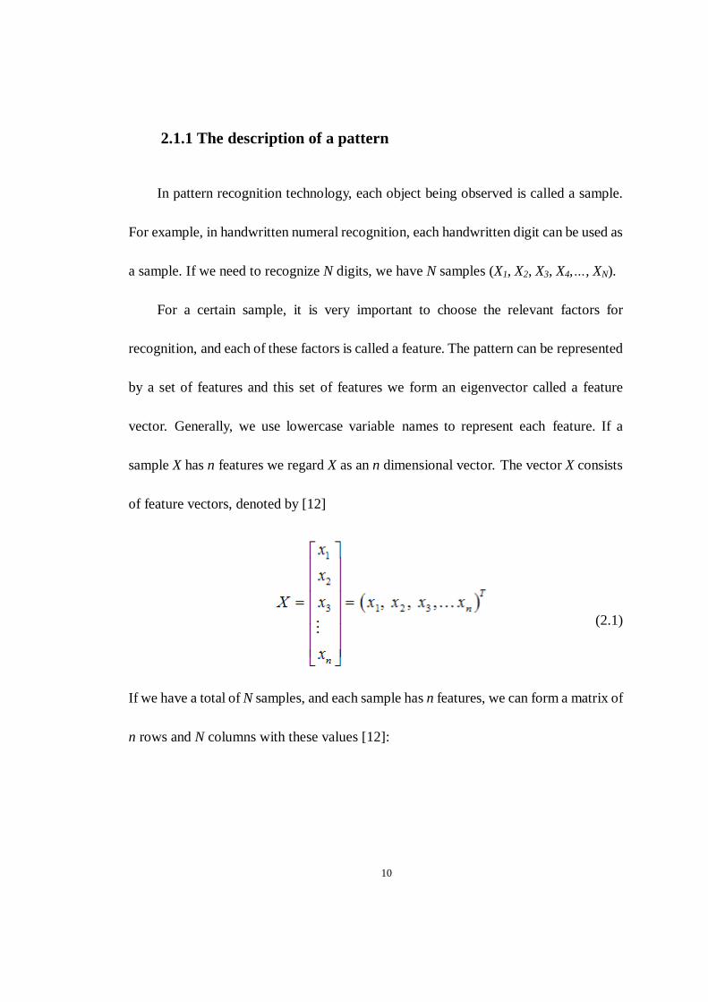
2.1.1 The description of a pattern

In pattern recognition technology, each object being observed is called a sample.

For example, in handwritten numeral recognition, each handwritten digit can be used as

a sample. If we need to recognize N digits, we have N samples (X1, X2, X3, X4,…, XN).

For a certain sample, it is very important to choose the relevant factors for

recognition, and each of these factors is called a feature. The pattern can be represented

by a set of features and this set of features we form an eigenvector called a feature

vector. Generally, we use lowercase variable names to represent each feature. If a

sample X has n features we regard X as an n dimensional vector. The vector X consists

of feature vectors, denoted by [12]

(2.1)

If we have a total of N samples, and each sample has n features, we can form a matrix of

n rows and N columns with these values [12]:

11

(2.2)

2.1.2 Pattern recognition system

A typical pattern recognition system is made up of data mining, preprocessing,

feature extraction, feature clustering, and a classifier. Figure 3 depicts pattern

recognition in the form of a flow chart.

Data mining

Preprocessing

Feature extraction

Classification

Figure 3 Component units of a pattern recognition system

12

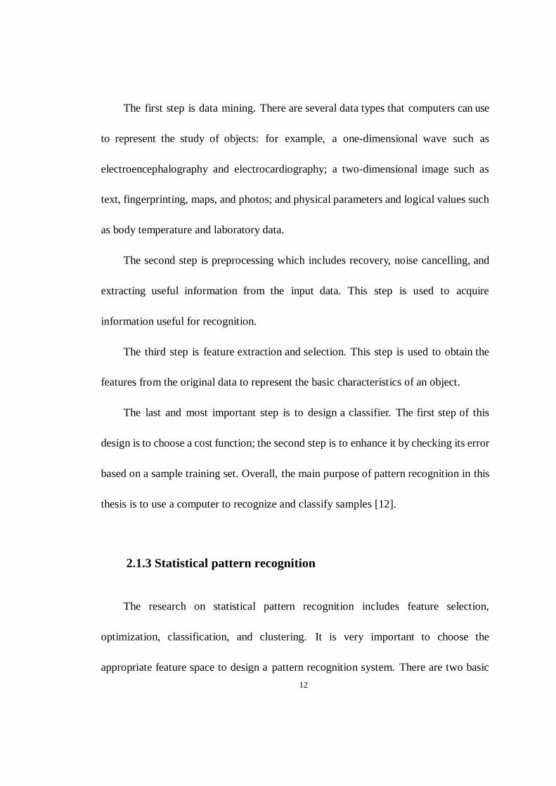
The first step is data mining. There are several data types that computers can use

to represent the study of objects: for example, a one-dimensional wave such as

electroencephalography and electrocardiography; a two-dimensional image such as

text, fingerprinting, maps, and photos; and physical parameters and logical values such

as body temperature and laboratory data.

The second step is preprocessing which includes recovery, noise cancelling, and

extracting useful information from the input data. This step is used to acquire

information useful for recognition.

The third step is feature extraction and selection. This step is used to obtain the

features from the original data to represent the basic characteristics of an object.

The last and most important step is to design a classifier. The first step of this

design is to choose a cost function; the second step is to enhance it by checking its error

based on a sample training set. Overall, the main purpose of pattern recognition in this

thesis is to use a computer to recognize and classify samples [12].

2.1.3 Statistical pattern recognition

The research on statistical pattern recognition includes feature selection,

optimization, classification, and clustering. It is very important to choose the

appropriate feature space to design a pattern recognition system. There are two basic

13

methods to optimize the choice of the feature space. One is feature selection and the

other is feature optimization. For example, if we want to identify oranges and apples,

we can select a feature by distinguishing them by shape or color, and then we still can

optimize the feature. As long as we observe them carefully then it’s not hard to find

out there is an easier way to tell the difference between apples and oranges by their

color than their shapes.

If we assume that we know some samples and their features, then one

classification problem is to recognize the Arabic numerals from zero to nine by

comparing them to a known sample in the database. By recognizing these digits, the

system must “know” the shape feature of each handwritten digit. One problem that

exists is that different people have different ways of writing each digit. Even the same

people may have different ways of writing the same digit. In this case we should let the

system know what category the digit belongs to. Therefore we should establish a

sample database.

2.2 Classifier design

The classification problem in pattern recognition is to assign an object into

different categories according to its observation value [42]. The steps are listed as

14

follows: (1) We establish a training set in feature space. (2) We suppose that we already

know every point’s type in the training set so that we may find the optimal cost

function or approach for pattern recognition. (3) After we choose an approach or a cost

function, then we can determine parameters according to those conditions. The

following sections discuss two separate approaches to classification.

2.2.1 Template matching

This method is based on the concept of similarity which is the simplest and most

straightforward method. In this method, we compare a pattern being classified with the

standard template to see which pattern has the highest similarity. For example, A class

has 10 training samples, thus it has 10 templates, while B class has 15 training samples

which means it has 15 templates. Then we try to classify the testing sample by

calculating the similarities between it and the 25 templates. If we find out it is similar

with one template in A class we confirm that the testing sample is A class, otherwise it is

B class. Theoretically the template matching approach is the simplest but its biggest

flaw is the large amount of calculation and large amount of storage needed. We need to

store quite a lot of templates and we need to compare each one many times, and this

leads to a lot of computation time.

15

2.2.2 Artificial neural networks

Training and machine learning is a scientific discipline that tries to find the

optimal solution for some mathematical formula based on a training set. This optimal

solution allows a classifier to obtain a group of parameters [25], and with this group of

parameters we can use the classifier to achieve the best performance.

When we talk about training or machine learning, we are likely to refer to several

concepts. The first one is a training set which is a known sample set. Like its name, we

use this known set to train a classifier. The second one is a test set which is an

independent sample set that has not been used during the design of the pattern

recognition system [25].

An artificial neural network is a mathematical model or computational model that

serves to imitate the way people think, and it is a non-linear and adaptive dynamic

system that changes its structure based on external or internal information. It consists of

an interconnected group of artificial neurons and processes information using a

connectionist approach to computation. Overall, a neural network satisfies many

desired features such as parallel processing, continuous adaption, fault tolerance, and

self-organization [19]. Therefore we can use artificial neural networks to solve the

non-normal distribution and non-linear problem effectively. Figure 4 shows the scheme

of a neural network.

16

Figure 4 The basic structure of a neural network, public domain image taken from

http://en.wikipedia.org/wiki/Artificial_neural_network

2.3 Feature recognition

In most cases, the input set is a multi-feature, high noise, and non-linear data set in

practical applications. There are some influential factors that we should consider such

as if the size of the training set is small. In this case we should use many features to

train a classifier, which leads to increasing the complexity and calculation. Therefore,

how to condense a high dimensional feature space becomes a big problem. Generally

speaking, there are two approaches; one is feature selection, and the other is feature

extraction.

17

2.3.1 Feature selection

Feature selection in pattern recognition is an important issue. The amount of data

that is obtained directly from the sample is usually very large [32]. For example, we

can have hundreds of thousands of characteristics in a normal image and the amount of

data of a satellite image is even more. In order to identify an object accurately we need

to select its features carefully. Feature selection is to extract those features that can be

distinguished from other features in the original data; therefore these features can

represent the nature of objects. If we can find these different types of features from the

input data we can simply translate pattern recognition to a look-up table problem,

which makes the problem much easier.

To design a classifier is to choose the kind of features that describe an object,

which is the same as choosing an appropriate feature space [42]. For example, color is

a feature to distinguish between red and green lights, because one object is red and the

other is green. We can easily tell the difference between a red light and a green light by

color. But it is very difficult to distinguish a human face if we try to use color as a

distinguishing feature.

We are often faced with keeping some data and abandoning others when we select

features especially if a large number of features is available. Therefore, we have to

choose features carefully which means that the feature size should not be too large or

18

too small. If the size is too large, it takes too much computation time; on the other hand

if it is too small it may be very difficult to recognize the object. In either case feature

selection is the process of choosing the most effective features from a set of features in

order to achieve the purpose of reducing the feature space [38].

2.3.2 Feature extraction

The definition of feature extraction is mapping or transforming a high

dimensional feature vector into a low dimensional feature vector [38]. The feature

vector obtained from feature extraction is a certain combination of the original feature

set and the new feature vector that includes all the information in the original feature

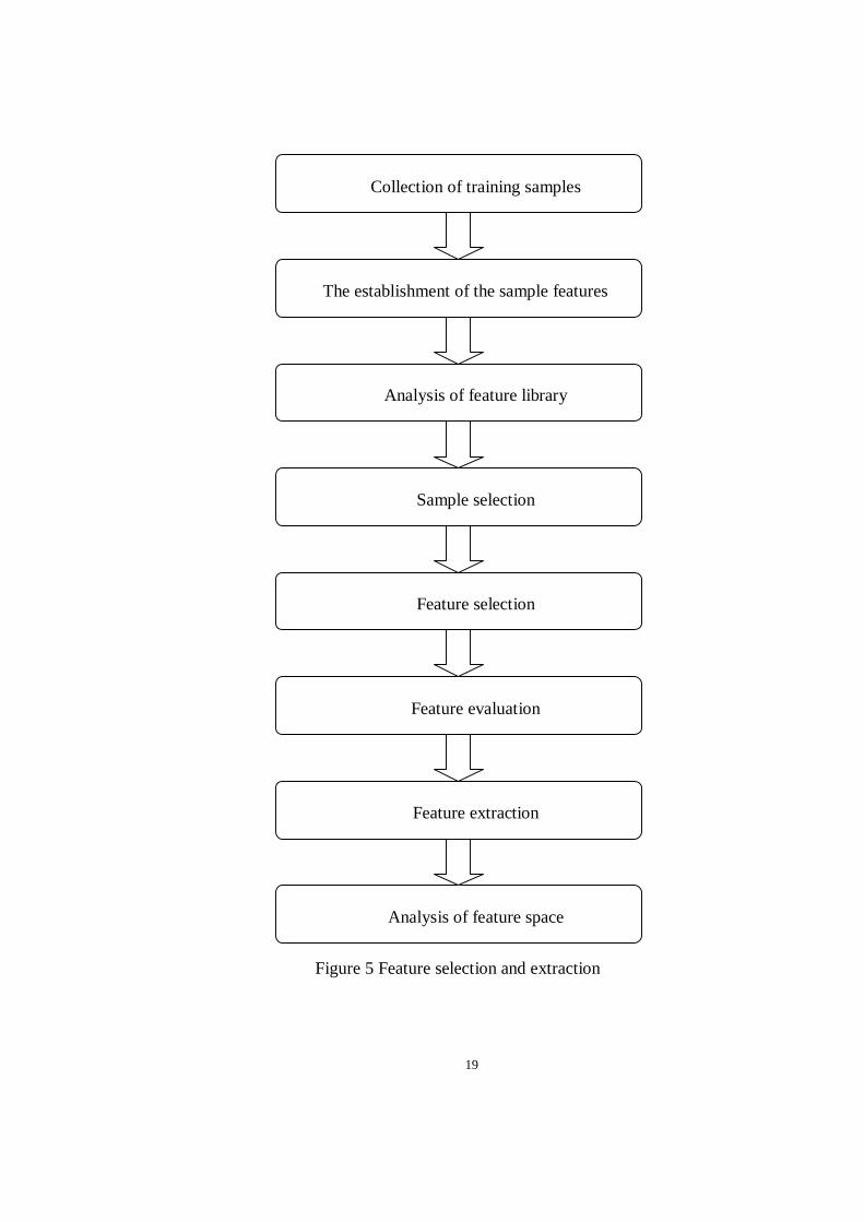
vector. Figure 5 shows the steps of feature selection and extraction.

19

Collection of training samples

The establishment of the sample features

Analysis of feature library

Sample selection

Feature selection

Feature evaluation

Feature extraction

Analysis of feature space

Figure 5 Feature selection and extraction

20

2.4 Numerical feature extraction and analysis

There are a few methods to extract numerical feature. Distance change method is

shown in Figure 6. As the method’s name implies, we keep track of the distance

between the left border and the number. We know the shape of the number from the

change of the distance [36].

Figure 6 Distance change method

The other method used in this thesis is n×m template extraction [36]. This method

is shown in Figure 7. We divide the image into n×m parts and each part has several

pixels which makes it a “super” pixel. Therefore there are n×m “super” pixels. The

main idea of this method is to regard the image as an n×m image, and then recognize it.

21

Figure 7 n×m template extraction method

Figure 8 n×m pixels

Figure 8 shows n×m super pixels. We first find the start position of each sample

and then find out the height and width of the sample. Second, we divide the height into

n parts and the width into m parts which makes an n×m region. For each region we need

to calculate the number of dark pixels in this area and then divide the number by area to

obtain the feature value. The greater the n×m value the more features, which also

means the higher the recognition rate may be, but at the same time it is more likely to

increase the calculation, the computation time, and the sample database size [36].

Generally speaking, the number of samples should be at least 10 times the number

of features [26]. Let’s suppose that we take n=6 and m=4. This means that we need at

22

least 4×6×10 samples for each digit. Therefore we have total 4×6×10×10 samples for

all 10 digits, which is quite a large number.

The benefit of the n×m template extraction method is that we can use it on

different size numbers, which suggests that we can regard those samples with different

sizes as the same type. We require that the height and width of the number should be at

least four pixels, or it may be too small to recognize.

2.5 Pattern similarity measure

The most basic research question of pattern recognition is the similarity

measurement between two samples. We often use the nearest neighbor method to

measure similarity, that is, we compare each pattern being recognized with standard

samples to see which sample has the highest similarity. In principle, the nearest

neighbor method is a template matching method. There are several approaches to

measure similarity: Euclidean distance, Mahalanobis distance, cosine angle distance

and Tanimoto measure of similarity [27].

23

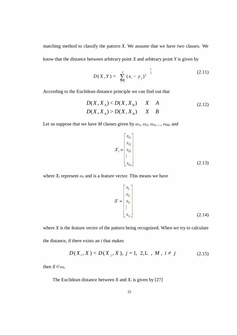
2.5.1 The distance between two patterns

Suppose that we have two patterns Xi and Xj and their feature vectors are

(2.3)

(2.4)

and the Euclidean distance is given by [27]

22

2

1

( ) ( )

( )

i j

TE i j i j i j

n

ik jkk

D X X X X X X

x x=

= − − = −

= −∑

(2.5)

If the DEij value is small then the distance between the two patterns is also small, which

means the similarity is high.

We can also find the distance with the Mahalanobis distance given by [27]

2 1( ) ( )i j

TM i j i jD X X S X X−= − − (2.6)

with the covariance matrix

1

1 ( )( )1

NT

i ii

S X X X XN =

= − −− ∑

(2.7)

24

1

1 N

ii

X XN =

= ∑

(2.8)

If the DMij value is small, then the distance between two patterns is also small, which

means the similarity is high.

Another way of finding the distance is by the cosine angle distance given by the

formula [27]

( ), cosTi j

C i j Ci j

X XS X X

X Xθ= =

⋅ (2.9)

If Sc is large this means the similarity between two patterns is high.

If all the features in a vector are binary values, then we use the Tanimoto measure

of similarity which is given by the formula [27]

( ), cosTi j

T i j T T T Ti i j j i j

X XS X X

X X X X X Xθ= =

+ −

(2.10)

If ST is large this means the similarity between two patterns is high.

2.5.2 Template matching method

Suppose we have a template A and a template B and there are n-dimensional

feature vectors which are given by XA=(XA1, XA2, XA3,…, XAn)T and XB=(XB1, XB2, XB3,…,

XBn)T, and the pattern being recognized is X=(X1, X2, X3,…, Xn)T. Let’s use the template

25

matching method to classify the pattern X. We assume that we have two classes. We

know that the distance between arbitrary point X and arbitrary point Y is given by

12

2

1( , ) ( )

n

i ji

D X Y x y=

= − ∑

(2.11)

According to the Euclidean distance principle we can find out that

( , ) ( , )( , ) ( , )

A B

A B

D X X D X X X AD X X D X X X B

< ⇒ ∈> ⇒ ∈

(2.12)

Let us suppose that we have M classes given by ω1, ω2, ω3,…, ωM, and

(2.13)

where Xi represent ωi and is a feature vector. This means we have

(2.14)

where X is the feature vector of the pattern being recognized. When we try to calculate

the distance, if there exists an i that makes

( , ) ( , ), 1, 2, , , i jD X X D X X j M i j< = ≠L (2.15)

then X∈ωi.

The Euclidean distance between X and Xi is given by [27]

26

2( , ) ( ) ( )

( )

Ti i i i

T T T Ti i i i

T T T Ti i i i

D X X X X X X X X

X X X X X X X XX X X X X X X X

= − = − −

= − − +

= − + −

(2.16)

27

CHAPTER III

IMAGE PROCESSING

Image processing is based on the principle of recognizing certain patterns within

an image. We can then use the image processing technology to obtain the information

that we are interested in. This thesis uses formulas to recognize certain patterns that

exist within an image. Therefore we now discuss image processing.

3.1 Image segmentation

Image segmentation is the most basic and the most important task in the image

processing system. The results of image segmentation affect feature extraction and

28

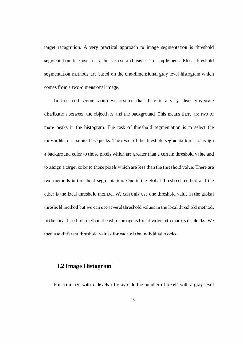
target recognition. A very practical approach to image segmentation is threshold

segmentation because it is the fastest and easiest to implement. Most threshold

segmentation methods are based on the one-dimensional gray level histogram which

comes from a two-dimensional image.

In threshold segmentation we assume that there is a very clear gray-scale

distribution between the objectives and the background. This means there are two or

more peaks in the histogram. The task of threshold segmentation is to select the

thresholds to separate these peaks. The result of the threshold segmentation is to assign

a background color to those pixels which are greater than a certain threshold value and

to assign a target color to those pixels which are less than the threshold value. There are

two methods in threshold segmentation. One is the global threshold method and the

other is the local threshold method. We can only use one threshold value in the global

threshold method but we can use several threshold values in the local threshold method.

In the local threshold method the whole image is first divided into many sub-blocks. We

then use different threshold values for each of the individual blocks.

3.2 Image Histogram

For an image with L levels of grayscale the number of pixels with a gray level

29

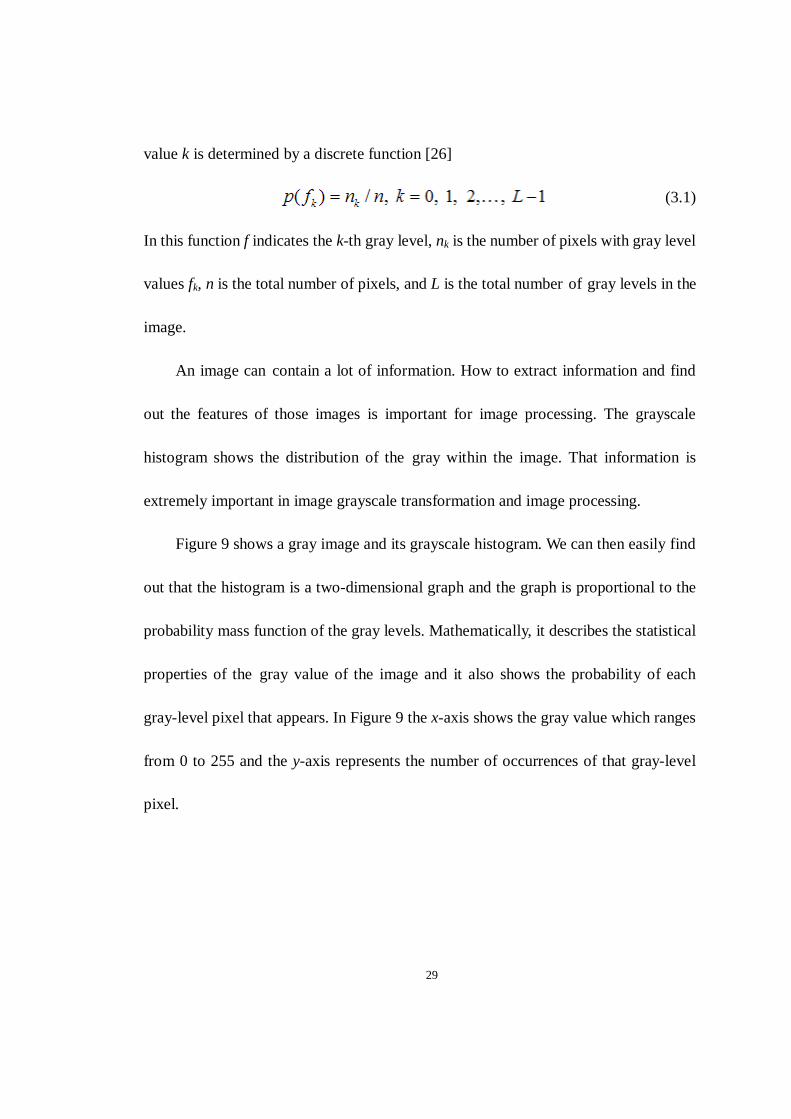
value k is determined by a discrete function [26]

(3.1)

In this function f indicates the k-th gray level, nk is the number of pixels with gray level

values fk, n is the total number of pixels, and L is the total number of gray levels in the

image.

An image can contain a lot of information. How to extract information and find

out the features of those images is important for image processing. The grayscale

histogram shows the distribution of the gray within the image. That information is

extremely important in image grayscale transformation and image processing.

Figure 9 shows a gray image and its grayscale histogram. We can then easily find

out that the histogram is a two-dimensional graph and the graph is proportional to the

probability mass function of the gray levels. Mathematically, it describes the statistical

properties of the gray value of the image and it also shows the probability of each

gray-level pixel that appears. In Figure 9 the x-axis shows the gray value which ranges

from 0 to 255 and the y-axis represents the number of occurrences of that gray-level

pixel.

30

Figure 9 A gray image and its histogram, public domain image taken from

http://book.csdn.net/bookfiles/974/10097430283.shtml.

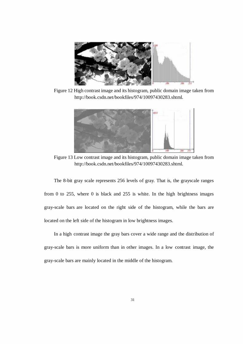
Figures 10, 11, 12, and 13 show four images acquired from the same image and

their grayscale histograms. They are high brightness, low brightness, high contrast, and

low contrast. The right side of each image is its corresponding histogram.

Figure 10 High brightness image and its histogram, public domain image taken

from http://book.csdn.net/bookfiles/974/10097430283.shtml.

Figure 11 Low brightness image and its histogram, public domain image taken

from http://book.csdn.net/bookfiles/974/10097430283.shtml

31

Figure 12 High contrast image and its histogram, public domain image taken from


Figure 13 Low contrast image and its histogram, public domain image taken from


The 8-bit gray scale represents 256 levels of gray. That is, the grayscale ranges

from 0 to 255, where 0 is black and 255 is white. In the high brightness images

gray-scale bars are located on the right side of the histogram, while the bars are

located on the left side of the histogram in low brightness images.

In a high contrast image the gray bars cover a wide range and the distribution of

gray-scale bars is more uniform than in other images. In a low contrast image, the

gray-scale bars are mainly located in the middle of the histogram.

32

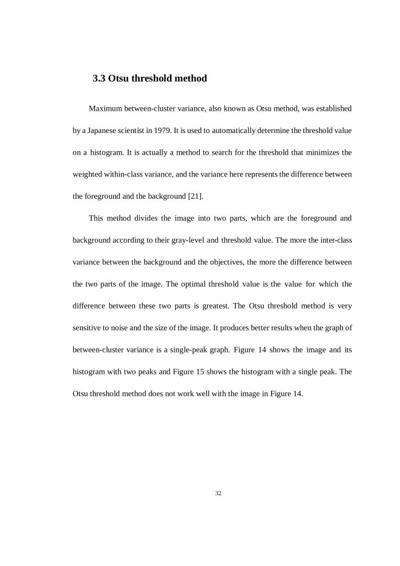
3.3 Otsu threshold method

Maximum between-cluster variance, also known as Otsu method, was established

by a Japanese scientist in 1979. It is used to automatically determine the threshold value

on a histogram. It is actually a method to search for the threshold that minimizes the

weighted within-class variance, and the variance here represents the difference between

the foreground and the background [21].

This method divides the image into two parts, which are the foreground and

background according to their gray-level and threshold value. The more the inter-class

variance between the background and the objectives, the more the difference between

the two parts of the image. The optimal threshold value is the value for which the

difference between these two parts is greatest. The Otsu threshold method is very

sensitive to noise and the size of the image. It produces better results when the graph of

between-cluster variance is a single-peak graph. Figure 14 shows the image and its

histogram with two peaks and Figure 15 shows the histogram with a single peak. The

Otsu threshold method does not work well with the image in Figure 14.

33

Figure 14 The histogram with two peaks

Figure 15 The histogram with a single peak

The Otsu threshold method is a global non-parametric, unsupervised, and

automatic threshold selection algorithm. If there are N pixels in a two-dimensional gray

image and the gray levels of those pixels are from 1 to L then the number of pixels at

level i is denoted by ni and the histogram of gray level is regarded as a distribution [33]

given by

/ , 0i i iP n N P= ≥

1

1L

ii

P=

=∑

(3.2)

(3.3)

Now suppose that we divide the pixels into class C1 and class C2 by the threshold

34

value k. If one of these classes is a background and the other one is an object then C1 has

gray levels given by [1,…, k] and C2 has levels given by [k+1,…, L]. Then the

probability distributions of the gray levels of these two classes are given by [33]

1 11

: ( ) ( )k

ii

C k P kω ω=

= =∑

(3.4)

2 21

: ( ) 1 ( )L

ii k

C k P kω ω= +

= = −∑

(3.5)

The mean gray levels for classes C1 and C2 are given by

1 11 1 1

( )Pr( | )( ) ( )

k ki

i i

iP ki i Ck k

µµ

ω ω= =

= = =∑ ∑

(3.6)

2 21 1 2

( )Pr( | )( ) 1 ( )

L Li L

i k i k

iP ki i Ck k

µ µµ

ω ω= + = +

−= = =

−∑ ∑ (3.7)

where

1( )

k

ii

k iPµ=

= ∑

(3.8)

1( )

L

L ii

L iPµ µ=

= = ∑ (3.9)

We can also easily verify the following relation

1 1 2 2 Lω µ ω µ µ+ =

1 2 1ω ω+ =

(3.10)

(3.11)

35

The class variances are given by [33]

2 2 21 1 1 1 1

1 1( ) Pr( | ) ( ) /

k k

ii i

i i C i Pσ µ µ ω= =

= − = −∑ ∑

(3.12)

2 2 22 2 2 2 2

1 1( ) Pr( | ) ( ) /

L L

ii k i k

i i C i Pσ µ µ ω= + = +

= − = −∑ ∑

(3.13)

We can use the Otsu discriminant analysis to define the between-class variance as [21]

1 2

1 2

1 2

1 2

1 2 1 1 2 2

1 2

2 2 21 1 2 2

2 2 2 21 1 1 1 2 2 2 2

2 2 21 2 1 1 2 2 1 2

2 2 2 21 2

2 2 21 2

2 2 2 2 2 21 2 1 1 2 2

2 21 1 2 2

( ) ( )

2 2

2 ( ) ( )

2

2

(1 ) (1 )

L

B L L

L L L L

L L

L

L

σ ω µ µ ω µ µ

ω µ ω µ µ ω µ ω µ ω µ µ ω µ

ω µ ω µ µ ω µ ω µ ω ω µ

ω µ ω µ µ µ

ω µ ω µ µ

ω µ ω µ ω µ ω µ ω µ ω µ

ω µ ω ω µ ω

= − + −

= − + + − +

= + − + + +

= + − +

= + −

= + − − −

= − + −

1 2

1 1 2 2

2 21 2 1 2 1 1 2 2

21 2 1 2

2

2

( )

ω µ ω µ

ω ω µ ω ω µ ω µ ω µ

ω ω µ µ

−

= + −

= −

(3.14)

According to the Otsu method if we choose an optimal k value so that σB2 is maximized

then [21]

2 2

1( ) max ( )B Bk Lk kσ σ

≤ ≤′ =

(3.15)

so that we can have best performance.

Figure 16 shows an original image to be transformed. If we use the Otsu threshold

method to transform the color image to a black and white image with different

36

threshold values then the images are shown in Figures 18, 19, and 20. Figure 17 shows

the histogram corresponding to Figure 16 (we use MATALB® to plot a gray-level

histogram).

Figure 16 Original utility meter image #1

Figure 17 Histogram of utility meter image #1

37

Figure 18 Black and white image with threshold value 64



From the black and white images with different threshold values we can easily see

that the threshold value is a very important factor for image processing. If the threshold

38

value is too large then the B&W image will be too dark, and if the value is too small

then the B&W image will be too light to recognize.

39

CHAPTER IV

SOFTWARE AND HARDWARE

4.1 Software

We use a computer language called Visual C#® to write an executable program

(see Figure 21). The software runs on all Windows® operating system platforms. In the

program there are five buttons: preprocessing, recognize, plot, cost and load as shown

in Figure 21.

40

Figure 21 User interface

When we click the preprocessing button the wireless camera will start to work and

the computer will obtain the image from the receiver and save the image in a special

location. The next step is to locate the number in the image when the red rectangle pops

up on the screen. When you finished locating the numbers by dragging the red

rectangles, the computer will save the coordinate of each number as a binary file. The

next time when it starts to recognize the number the computer will segment the number

with the coordinates that were saved. If we click the preprocessing button the computer

will “remember” the location of each digit. Therefore technically we do not need to

click it again unless someone has moved the camera or we want to test it.

41

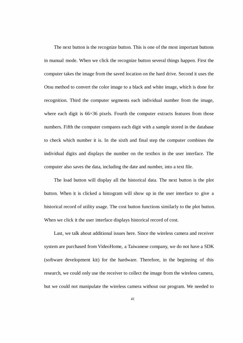
The next button is the recognize button. This is one of the most important buttons

in manual mode. When we click the recognize button several things happen. First the

computer takes the image from the saved location on the hard drive. Second it uses the

Otsu method to convert the color image to a black and white image, which is done for

recognition. Third the computer segments each individual number from the image,

where each digit is 66×36 pixels. Fourth the computer extracts features from those

numbers. Fifth the computer compares each digit with a sample stored in the database

to check which number it is. In the sixth and final step the computer combines the

individual digits and displays the number on the textbox in the user interface. The

computer also saves the data, including the date and number, into a text file.

The load button will display all the historical data. The next button is the plot

button. When it is clicked a histogram will show up in the user interface to give a

historical record of utility usage. The cost button functions similarly to the plot button.

When we click it the user interface displays historical record of cost.

Last, we talk about additional issues here. Since the wireless camera and receiver

system are purchased from VideoHome, a Taiwanese company, we do not have a SDK

(software development kit) for the hardware. Therefore, in the beginning of this

research, we could only use the receiver to collect the image from the wireless camera,

but we could not manipulate the wireless camera without our program. We needed to

42

connect the hardware with the software. We found a C#® class (open source) which is

developed by Microsoft online, and this C#® class can control the wireless camera. This

class is named “GetVideo” which is a very universal class; it can manipulate a lot of

cameras no matter what brand they are. All we needed to do was to change some

parameters in the class to achieve our goal.

Another issue was that when we tried to plot the histogram in the C# environment,

we found out that there was not any controller in the standard toolbox that met our

requirement. We found a free controller called “zedgraph” that worked well with the

code.

Even though we have finished the thesis, we still find the research has room for

additional work, which we discuss in the following section.

4.2 Hardware

The camera (Figure 22) that we use has a wireless radio built in to it. It is made by

a Taiwanese company called VideoHome Technology (www.videohome.com.tw). We

bought our camera from a distributor called SuperDroid Robots that specializes in

robotics equipment (www.superdroidrobots.com). The camera costs $33 and has a

built-in transmitter (SuperDroid part # WC-046-000). The receiver (Figure 23) costs

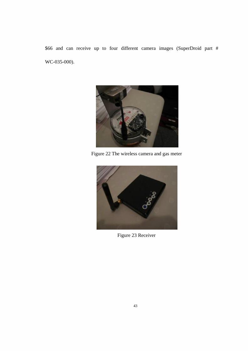
43

$66 and can receive up to four different camera images (SuperDroid part #

WC-035-000).

Figure 22 The wireless camera and gas meter

Figure 23 Receiver

44

CHAPTER V

EXPERIMENTAL RESULTS

45

In this chapter, we present experimental results based on the steps shown in Figure

24.

Read image from wireless camera

Convert color image to grayscale image

Convert grayscale image to B&W image

Edge detection

Extract features

Number recognition

Figure 24 The basic process of the automatic meter reading system

46

5.1 Conversion of color to grayscale

Since the color in a number does not contain any information, we need to convert

the color to black and white image (or gray image) so that the image is readable. If each

pixel in the image is a single sample, we call this image a grayscale image. A grayscale

image carries only intensity information which means that the value of red, green and

blue of each pixel are equal (while the RGB values of each pixel in a color image are

different). Figure 25 shows the original image and Figure 26 shows the result after

conversion. There are several approaches to convert a color image to a grayscale image.

In this thesis we use the following formula [8]

( )11 16 5 32R G B× + × + ×

(5.1)

where R, G, and B are the red value, green value and blue value of each pixel

respectively. This method is called the luminosity method. This formula is formed

based on human perception. Because humans are more sensitive to green than other

colors, green is weighted most heavily [8].

47

Figure 25 Original utility meter image #2

Figure 26 Grayscale image

5.2 Image binarization (conversion of grayscale to black and

white)

After we convert the color image to a grayscale image, each pixel of the image has

only one value, and we call this value the grayscale. This grayscale value denotes the

luminance level. For further recognition, we still need to convert grayscale to binary

48

(black and white image). Here, we use the Otsu threshold method to find the threshold

value and then convert it. We have already discussed the concept of the Otsu threshold

method in detail in former chapters, so we do not talk about it here. After binarization,

we obtain the image shown in Figure 27.

Figure 27 Black and white image

5.3 Edge detection and number segment detection

The edge detection we use here is a little different than that to which people

usually refer. Edge detection is a basic problem in image processing and computer

vision; edge detection aims to point out where the brightness of digital images changes

sharply. Instead of automatic detection, we use manual detection. Generally speaking,

the utility meter is located outside of the house, which means when we collect the data

from the meter we may face different weather situations. Therefore we derive a new

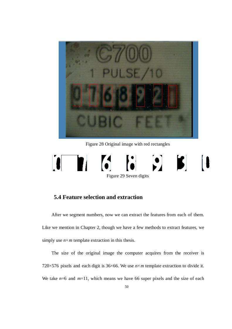
approach here. As Figure 28 shows, we create some rectangles to locate the numbers,

49

with which we can increase the recognition rate.

In a way this is manual recognition, however, after the system is calibrated, it is

automatic recognition. We locate the numbers manually the first time; after that the

computer can “remember” the location, and locate digits according to last manual

calibration. Therefore, this is still an automatic recognition. In our program, we simply

click the preprocessing button, then the image will appear with those rectangles. Then

we can move these rectangles by clicking and dragging with the computer mouse to

locate the number areas, and the computer will save the locations automatically. Next

time you click the recognition button, the program will crop the number areas based

on the saved locations. Figure 28 shows the original image with red rectangles and

Figure 28 shows the result after image binarization and number segmentation.

50

Figure 28 Original image with red rectangles

Figure 29 Seven digits

5.4 Feature selection and extraction

After we segment numbers, now we can extract the features from each of them.

Like we mention in Chapter 2, though we have a few methods to extract features, we

simply use n×m template extraction in this thesis.

The size of the original image the computer acquires from the receiver is

720×576 pixels and each digit is 36×66. We use n×m template extraction to divide it.

We take n=6 and m=11, which means we have 66 super pixels and the size of each

51

super pixel is 6×6. Here, we explain why we chose the super pixel as 6×6. The factors

of 36 are 1, 2, 3, 4, 6, 9, 12, 18 and 36, and the factors of 66 are 1, 2, 6, 11, 33, and 66.

So there are 9×6=54 possible combinations of n and m. If n and m are too small, it

will take too much computation time, and if n and m are too large, the number of

feature will not be enough for recognition. We have tested all of 54 combinations, and

found that the result of 6×6 is the best balance between accuracy and computation

time. We calculated the sum of pixels of each 6×6 area to obtain 66 super pixel values,

and then we used these 66 values as the features. Figure 30 shows that the number has

66 features.

Figure 30 6×11 features

After we extract the features, we input these into a matrix to compare with samples

previously saved in order to choose the sample which has the highest similarity. We

save all the features as binary matrix format, that is, the each element of the matrix is

equal to 0 or 1. 1 represents white, and 0 represents black. Since number recognition is

52

based on black and white images, the matrix is binary.

5.5 Number recognition

Now that we have collected the information we need to recognize, the next step is

to recognize the number. All we need is a classifier. A classifier is a black box which we

input some information into, and then the result we want will be output. In this case we

input features, and the classifier outputs the number. Since we talk about classifiers in

Chapter 2, we do not go into detail here, but we summarize our approach in the

following paragraph.

There are several approaches to design a classifier, such as template matching,

artificial neural network, probabilistic approach, etc. We choose template matching in

this thesis because it is easy to understand, and every step of template matching is

very clear. If some step of template matching goes wrong, we can easily find out and

fix it. However, since this method leads to large amount of calculation and large

amount of storage, it may take more time than other methods as a disadvantage. After

testing hundreds of samples, we find the average recognition time is about 30 seconds,

which is acceptable for AMR.

Since we use template matching, we should calculate the distance between two

53

patterns. Therefore we decide to use Euclidean distance to calculate the distance. The

formula is shown below [27]

22

2

1

( ) ( )

( )

i j

Ti j i j i j

n

ik jkk

D X X X X X X

x x=

= − − = −

= −∑

(5.2)

where Xi is the pattern being recognized and Xj is the sample. The basic rule of this

approach is to check which Dij2 is smallest.

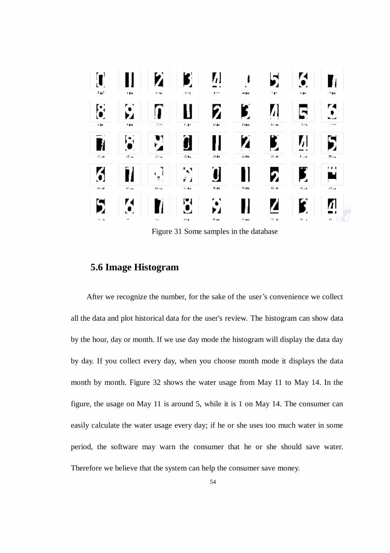
We have about 200 standard samples in our database and we can use the features

of those samples to compare with the features of the patterns. Simply speaking, we put

the feature value into the formula above. Figure 31 shows some of our sample

database.

54

Figure 31 Some samples in the database

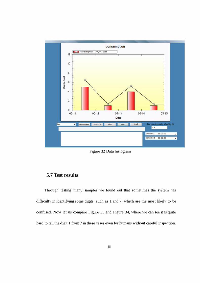
5.6 Image Histogram

After we recognize the number, for the sake of the user’s convenience we collect

all the data and plot historical data for the user's review. The histogram can show data

by the hour, day or month. If we use day mode the histogram will display the data day

by day. If you collect every day, when you choose month mode it displays the data

month by month. Figure 32 shows the water usage from May 11 to May 14. In the

figure, the usage on May 11 is around 5, while it is 1 on May 14. The consumer can

easily calculate the water usage every day; if he or she uses too much water in some

period, the software may warn the consumer that he or she should save water.

Therefore we believe that the system can help the consumer save money.

55

Figure 32 Data histogram

5.7 Test results

Through testing many samples we found out that sometimes the system has

difficulty in identifying some digits, such as 1 and 7, which are the most likely to be

confused. Now let us compare Figure 33 and Figure 34, where we can see it is quite

hard to tell the digit 1 from 7 in these cases even for humans without careful inspection.

56

Figure 33 Digit seven

Figure 34 Digit one

We have tested 105 samples in a regular environment, which means the light

intensity is not too high nor too low. Eight samples failed to be recognized in the test.

Therefore, the correct recognition rate is 92.3%. Each digit has a different recognition

rate; Table I shows the correct recognition rate of each sample.

Table I Digit recognition test results

Digit Number of correctly identified

Number of images

Recognition rate (%)

0 15 15 100% 1 11 11 100% 2 9 10 90% 3 7 8 87% 4 6 7 86% 5 10 10 100% 6 10 11 91% 7 11 14 78% 8 9 10 90% 9 14 14 100%

Correct recognition rate 92.3%

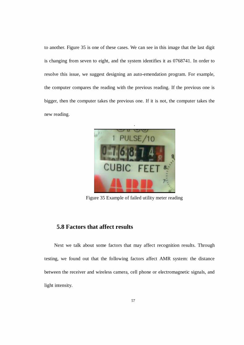
Most cases of recognition failure happen when the digit is transitioning from one

57

to another. Figure 35 is one of these cases. We can see in this image that the last digit

is changing from seven to eight, and the system identifies it as 0768741. In order to

resolve this issue, we suggest designing an auto-emendation program. For example,

the computer compares the reading with the previous reading. If the previous one is

bigger, then the computer takes the previous one. If it is not, the computer takes the

new reading.

.

Figure 35 Example of failed utility meter reading

5.8 Factors that affect results

Next we talk about some factors that may affect recognition results. Through

testing, we found out that the following factors affect AMR system: the distance

between the receiver and wireless camera, cell phone or electromagnetic signals, and

light intensity.

58

5.8.1 Effect of radio distance

Table II shows how distance affects the radio. We should also note that while the

images in Table II seem not as clear as that in Figure 35, this is due to the low light

intensity test environment.

Table II The effect of transmitter/receiver distance on the wireless camera signal

Distance (m) Image Clarity 0.5 m

Very clear

1 m

Very clear

2 m

Very clear

5m

Clear

59

8 m

Clear enough

10 m

Cannot be recognized

12 m


15 m


18 m

Lost connection

From Table II we can find that the result is very good when the

transmitter/receiver distance is within 5 m, and the receiver can still receive a clear

Table II (continued)

60

image from the wireless camera when the distance is between 5 m and 8 m (although

sometimes the result may be wrong), but once the distance extends to more than 8 m,

the image we acquire from the wireless camera is very fuzzy and cannot be

recognized. When the distance approaches 18 m, the receiver loses connection with

the wireless camera.

5.8.2 Effect of electromagnetic interference

The second factor that affects the results is the radio interference, which may be

influenced by cell phone and electromagnetic signals. We used a cell phone close to

the wireless camera and receiver to test the interference with the radio, and we found

that the signal would affect the radio only if the distance between the cell phone and

the wireless camera was below 30 cm. Table III shows the distance between cell

phone and receiver, and its effect on the image.

61

Table III The effect of electromagnetic interference on the wireless camera signal

Distance (cm) Image Clarity 0 cm

Hard to recognize

20 cm

May be recognized

30 cm

Very clear

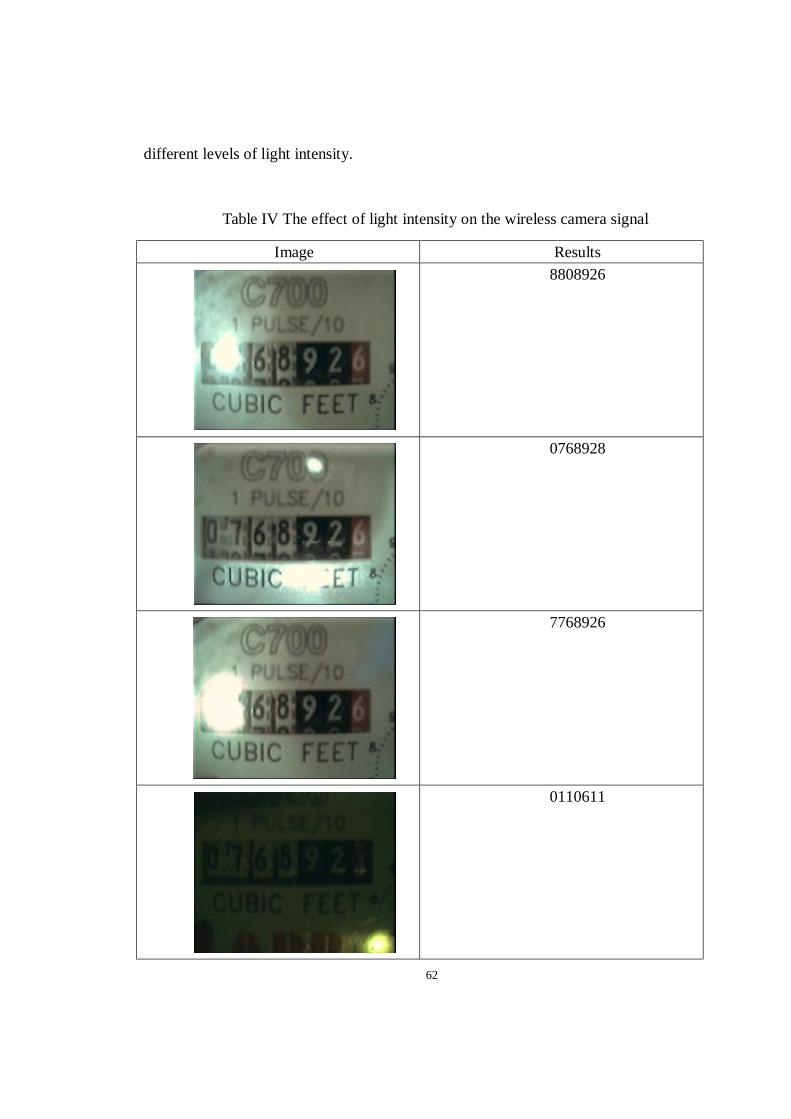
5.8.3 Effect of light intensity

The last but most important factor affecting the radio is light intensity. Though

we could not measure how bright conditions had to be for the system to no longer

function properly, we still want illustrate the problem through some images. Table IV

shows some images the system could not recognize because of too bright or too dark.

In the future we may add an external light so that the wireless camera can work in

62

different levels of light intensity.

Table IV The effect of light intensity on the wireless camera signal

Image Results

8808926

0768928

7768926

0110611

63

CHAPTER VI

CONCLUSION

6.1 Summary

The main technology we used in the thesis is pattern recognition. Pattern

recognition, which is one field in machine learning, is used in this thesis to recognize

the number on the utility meter. Pattern recognition is "the act of taking in raw data and

taking an action based on the category of the data" [15]. It is meant to classify different

information into different groups based on prior knowledge. In this thesis, the prior

knowledge is the sample database in the program. The machine “learns" knowledge

from the sample database so that it can distinguish the number on the meter. There are a

64

lot of basic methodologies in pattern recognition; in this thesis we used our own

technology, such as a red rectangle which helps the system to segment the number and

that increases the recognition rate. In many pattern recognition cases, we cannot use

this red rectangle technology because people may require all the steps to be automatic.

But in this special case of AMR, it is a good approach to implement, since we just need

to set the “rectangle” the first time.

Another technology that we use in this thesis is classifier design, which functions

like a black box. This process will tell you the result without the user needing to know

what is going on in the black box.

Another technology we used in the thesis is image binarization process. This

process was designed to convert the color picture to a black and white picture so that

the system can recognize the number. To convert the color picture to a black and white

picture we used the method called the Otsu threshold method to find the threshold in

order to finish conversion. This method is very popular in computer vision and image

processing.

6.2 Future work

First of all, we can’t apply the design to any environment which is too dark or light

65

because both these situations would affect the image binarization. In order to let the

wireless camera work in different levels of light intensity, we think there may be two

ways to solve the problem. One way is to improve the algorithm to work in different

levels of light intensity, and the other way is to add a light so every time we run the

program the wireless camera works in the same light intensity.

Second, we now can only recognize one utility meter at a time: what if a

consumer wants to check several meters at once? We are thinking of improving our

code in order to control four wireless cameras at the same time. The hardware can

manipulate four wireless cameras simultaneously, which means we don’t need to

change the hardware

Third, we need a base station which is a computer to analyze and present the

results, which means a consumer need to sit in front of the computer to check the

utility usage. For the sake of convenience, we are thinking of adding an Internet

function to our device. For example, we can use some software to send the results to

the consumer’s cell phone so that he or she can check the utility usage immediately,

no matter where they are.

Fourth, the system cannot recognize an analog style meter, such as a gas meter

(most gas meters in U.S. are analog as Figure 2 shows). We will change our

recognition method to meet this requirement; for instance, we may change from

66

template matching to a neural network.

Fifth, the system still fails to recognize numbers sometimes, for instance, the

number in Figure 36. We can see in the figure that the number is transitioning from 1

to 2. Therefore how to reduce the probability of that kind of error occurring becomes a

very important job. We suggest that we can extend our sample database to help solve

this problem

Figure 36 Reading during a transition from 1 to 2

6.3 Cost and benefits

Finally we will talk about the cost of the product and how much a utility can

company may save by using it. The product includes the receiver, the wireless camera,

the fixture to hold the wireless camera, and the external light source. The receiver

costs $66; the camera costs $33; the mechanical fixturing costs $5; the light costs an

estimated $10. Generally speaking, a customer has a gas, water and electricity meter,

and when we manufacture this AMR in quantity, we can get a 50% volume discount

for each component of the product. Therefore the product will cost around ($66+3×

67

($33+$5+$10)) ×50%=$105. Based on how much money it costs to employ human

meter readers and to obtain meter readings, a utility company may be able to save a

substantial amount of money by using this AMR system.

Finally, the installation of AMR will include other benefits beyond the monetary

ones. For example, hard-to-access meters can be read without difficulty and without

worrying about fences and animals. Reader errors will be reduced, which will increase

customer satisfaction. Customers will be able to monitor their utility usage in

real-time and remotely, which will give them a feeling of more control over their

utility usage. Leaks will be able to be detected more easily.

68

BIBLIOGRAPHY

[1] American Chronicle, Caller ID History,

http://www.americanchronicle.com/articles/view/66871, July 2008.

[2] A. Amin and S. Singh, Optical Character Recognition: Neural Network Analysis of

Hand-Printed Characters, Lecture Notes in Computer Science, vol. 1451, pp.

492-499, 1998.

[3] A. Amin and S. Singh, Neural Network Recognition of Hand-Printer Characters,

Neural Computing & Applications, vol. 8, pp. 67-76, March 1999.

[4] P. Belhumeur, J. Hespanha, and D. Kriegman, Eigenfaces vs. Fisherfaces:

Recognition using class specific linear projection, IEEE Transactions on Pattern

Analysis and Machine Intelligence, vol. 19, pp. 711-720, 1997.

[5] Keith Benman, The danger of being a meter reader,

http://nwitimes.com/news/local/article_e4947cc2-2279-5ce3-b217-522f2b55b49

a.html, Jan, 2010.

[6] J. Canny, A Computational Approach to Edge Detection, IEEE Transactions on

Pattern Analysis and Machine Intelligence, vol. 8, pp. 679-714, 1986.

69

[7] L. Cao, J. Tian and Y. Liu, Remote Real Time Automatic Meter Reading System

Based on Wireless Sensor Networks, 3rd International Conference on Innovative

Computing Information and Control, pp. 591-591, June 2008.

[8] J. Cook, Three algorithms for converting color to grayscale,

http://www.johndcook.com/blog/2009/08/24/algorithms-convert-color-grayscale,

August 2009.

[9] H. Deitel, P. Deitel, J. Listfield, T. Nieto, C. Yaeger, and M. Zlatkina, C#: A

Programmer's Introduction, Prentice Hall PTR, 1st edition, July 2002.

[10] F. Derbel, Smart Metering Based on Automated Meter Reading, 5th International

Multi-Conference on Systems, Signals and Devices July 2008.

[11] Y. Du, C. Chang and P. Thouin, An unsupervised approach to color video

thresholding, IEEE Conference on Pattern Recognition, vol. 11, pp. 919-922,

2002.

[12] R. Duda, P. Hart and D. Stork, Pattern Classification, Wiley-Interscience, 2nd

edition, October 2000.

[13] A. Gudessen, Quantitative Analysis of Preprocessing Techniques for the

Recognition of Hand Printed Characters, Pattern Recognition, vol. 8, pp. 219-227,

1976.

70

[14] M. Hamanaka, K. Yamada and J. Tsukumo, Normalization Cooperated Feature

Extraction Method for Hand Printed Kanji Character Recognition, Proceedings of

the Third International Workshop on Frontiers of Handwriting Recognition, pp.

343-348, 1993.

[15] D. Huang and C. Wang, Optimal Multi-level Thresholding Using a two-stage Otsu

Optimization Approach, Pattern Recognition Letters, vol. 30, pp. 275-284,

February 2009.

[16] Y. Huang, S. Lai, and W. Chuang, A Template Based Model for License Plate

Recognition, IEEE International Conference on Networking, Sensing and Control,

pp. 737-742, 2004.

[17] Johanson Technology, Inc, Automated Meter Reading,

http://www.johansontechnology.com/images/stories/tech-notes/ip/amr/Johanson_

Technology_AMR.pdf, July 2009.

[18] J. Kauffman, D. Sussman and C. Ullman, Beginning ASP.NET 2.0 with C#, Wrox,

May 2006.

[19] B. Kosko, Neural Network and Fuzzy Systems, Prentice Hall, 1992.

[20] K. Lee, J. Ho, M. Yang, and D. Kriegman, Video-based face recognition using

probabilistic appearance manifolds, IEEE Conference on Computer Vision and

Pattern Recognition, vol. 1, pp. 313-320, 2003.

71

[21] P. Liao, T. Chen and P. Chung, A Fast Algorithm for Multilevel Thresholding,

Journal of Information Science and Engineering, vol. 17, pp. 713-727, 2001.

[22] T. Lim and T. Chan, Experimenting Remote Kilowatt hour Meter Reading

Through Low-voltage Power Lines at Dense Housing Estates, IEEE Transactions

on Power Delivery, vol. 17, No. 3, July 2002.

[23] C. Liu, K. Nakashima, H. Sako and H. Fujisawa, Handwritten digit recognition:

investigation of normalization and feature extraction techniques, Pattern

Recognition, vol. 37, pp. 264-279, 2004.

[24] H. Maarif and S. Sardy, Plate Number Recognition by Using Artificial Neural

Network, http://komputasi.inn.bppt.go.id/semiloka06/Haris.pdf, 2006.

[25] T. Mitchell, The Discipline of Machine Learning,

http://www.cs.cmu.edu/~tom/pubs/MachineLearning.pdf, July 2006.

[26] P. Mitra, Pattern Recognition Algorithms for Data Mining, Taylor & Francis, 1st

edition, April 2007.

[27] G. Qian, S. Sural, Y. Gu and S. Pramanik, Similarity Between Euclidean and

Cosine Angle Distance for Nearest Neighbor Queries, Proceedings of the 2004

ACM Symposium on Applied Computing, pp. 1232 -1237, 2004.

[28] R. Medina and F. Madrid, Unimodal Thresholding for Edge Detection, Pattern

Recognition, vol. 41, pp. 2337-2346, 2008.

72

[29] Salary Wizard, Base Salary,

http://swz.salary.com/salarywizard/layouthtmls/swzl_compresult_national_sc160

00098.html, November 2009.

[30] T. Miller, Automated Meter Reading.

http://www.hawkeyerec.com/downloads/ARM_Meter_Article.pdf, August 2006.

[31] H. Ng, Automatic thresholding for defect detection, Pattern Recognition Letters,

vol. 27, pp. 1644-1649, 2006.

[32] L. Olivera, and R. Sabourin, A Methodology for Feature Selection using

Multi-objective Genetic Algorithms for Handwritten Digit String Recognition,

International Journal of Pattern Recognition and Artificial Intelligence, vol. 17,

No. 6, pp. 903-929, 2003.

[33] N. Otsu, A Threshold Selection Method from Gray-Level Histograms, IEEE

Transaction on Systems, man and Cybernetics, vol. 9, pp. 62-66, January 1979.

[34] F. Rasheed, T. Nestenius, J. Worthington and L. Addy, Programmer’s Heaven C#

School, Synchron Data, 1st edition, 2005.

[35] W. Siedlecki, and J. Sklansky, A Note on Genetic Algorithms for Large Scale on

Feature Selection, Pattern Recognition Letters, vol. 10, pp. 335-347, 1989.

73

[36] C. Suen, C. Nadal, R. Legault, A. Mai and L. Lam, Computer recognition of

unconstrained handwritten numerals, Proceedings of the IEEE, vol. 80, pp.

1162-1180, 1992.

[37] B. Tanner, K. Schacht, P. Jordan, P. Chappell and B. Pilling, What is automatic

meter reading?

http://docs.google.com/viewer?a=v&q=cache:9iC9jqJh1FgJ:www.epud.org/docu

ments/Creswell-Jan07_000.pdf+http://www.epud.org/documents/Creswell-Jan07

_000.pdf&hl=en&gl=us&sig=AHIEtbQC4r2RmaeqaOUrEWrpgtcAl-USZA,

February 2007.

[38] O. Trier, A. Jain and T. Taxt, Feature Extraction Methods for Character

Recognition—A Survey, Pattern Recognition, vol. 29, pp. 641-662, 1996.

[39] J. Tsukumo and H. Tanaka, Classification of Hand Printed Chinese Characters

using Nonlinear Normalization and Correlation Methods, Proceedings of the

Ninth International Conference on Pattern Recognition, pp. 168-171, 1998.

[40] Y. Yanamura, M. Goto, D. Nishiyama, M. Soga, H. Nakatani, and H. Saji,

Extraction and Tracking of the License Plate using Hough Transform and Voted

Block Matching, Proceedings of the IEEE Intelligent Vehicles Symposium, pp.

243-246, 2003.

74

[41] J. Zhang and J. Hu, Image Segmentation Based on 2D Otsu Method with

Histogram Analysis, International Conference on Computer Science and Software

Engineering, vol. 6, pp. 105-108, 2008.

[42] L. Zheng and X. He, Classification Techniques in Pattern Recognition,

http://wscg.zcu.cz/wscg2005/papers_2005/poster/k43-full.pdf, 2007.

AUTOMATIC UTILITY METER READING KAICHENG XIE · meter. Automatic meter reading (AMR) is used to...

Documents

Transcript of AUTOMATIC UTILITY METER READING KAICHENG XIE · meter. Automatic meter reading (AMR) is used to...