Automatic Urban Sound ClassificationUsing Feature Learning Techniques

Christopher B. Jacoby

Submitted in partial fulfillment of the requirements for theMaster of Music in Music Technology

in the Department of Music and Performing Arts ProfessionsSteinhardt School

New York UniversityAdvisor: Dr. Juan P. Bello

April 28, 2014

Abstract

Automatic sound classification is a burgeoning field in audio informat-

ics, which has been growing in parallel to developments in machine learn-

ing and urban informatics. In this thesis, we define two primary bottlenecks

to research in automatic urban sound classification: the lack of an estab-

lished taxonomy, and the meager supply of annotated real-world data. We

begin by assembling a new taxonomy of urban sounds to create a foundation

for future work in urban sound classification, which is an evolution on pre-

vious perceptually-focused environmental sound taxonomies. We describe

the process of curating a sizable dataset of real-world acoustic sounds col-

lected from the Freesound archive. The completed dataset, aptly dubbed Ur-

banSound, contains 27 hours of audio, with 18.5 hours of annotated events

across 10 classes. We further prepare a subset of the dataset which is sepa-

rated into 10 folds for cross-validation.

We begin analysis of our dataset with a baseline classification system us-

ing the off-the-shelf tools Essentia and Weka. Our baseline approach, based

on a typical MFCCs and a Support Vector Machine with Gaussian kernel,

gets just over 70% overall classification accuracy. We then take an estab-

lished algorithm for feature learning, which has been applied effectively in

image recognition and music informatics, and apply it to the classification

of urban environmental sounds. We compare the results of using of Spheri-

cal k-Means to traditional k-Means, and additionally compare the results of

those to static (not learned) random bases in order to prove that our feature

learning algorithm is learning useful features. While our feature learning

system does not outperform our baseline system overall, when we carefully

review the results at a per-class level, we discover that our system is indeed

performing better than the baseline for many of the classes, and in some

cases much better. The feature learning system improves the results of the

background classes over the random bases, and therefore some useful fea-

tures are learned by the system.

2

Acknowledgements

The author wishes to thank the following people:

Justin Salamon, Juan Bello, Tae Hong Park, Tlacael Esparza, Eric Humphrey,

whose collaboration and guidance made this work possible.

NYU faculty and cohorts: Paul Geluso, Agnieszka Roginska, Kenneth Pea-

cock, Uri Nieto, Rachel Bittner, Ethan Hein, John Turner, Alex Marse,

Michael Musick, Charlie Mydlarz, Jun Hee Lee, Allen Fogelsanger, Amar

Lal, and Akshay Kumar.

Friends, etc: Ross, Ross, Bryan, Chantae, Kit, Mog, Corey, Lynda, Robert,

Rowan, the Bouwerie Boys, Braintrust, Skip Wilkins, Larry Stockton, Jen-

nifer Kelly, Ismail Jouny, Oscar Bettison, Dan Trueman, and Jeff Snyder.

And finally: Meghan, Mom & Dad, and the rest of the family.

3

Contents

1 Introduction 7

2 A Taxonomy of Urban Sounds 112.1 Prior Work . . . . . . . . . . . . . . . . . . . . . . . . . . . . . . 11

2.1.1 Perception of Environmental Sounds . . . . . . . . . . . . 112.1.2 Environmental Sound Taxonomies . . . . . . . . . . . . . 12

2.2 Process . . . . . . . . . . . . . . . . . . . . . . . . . . . . . . . 132.2.1 Freesound Tags . . . . . . . . . . . . . . . . . . . . . . . 132.2.2 Sound Walks . . . . . . . . . . . . . . . . . . . . . . . . 142.2.3 311 Noise Complaints . . . . . . . . . . . . . . . . . . . 15

2.3 The Compiled Taxonomy . . . . . . . . . . . . . . . . . . . . . . 17

3 Dataset Creation 193.0.1 Data From Freesound . . . . . . . . . . . . . . . . . . . . 193.0.2 Phase 0: Download & Collect Raw Data . . . . . . . . . . 213.0.3 Phase 1: Select the Files . . . . . . . . . . . . . . . . . . 213.0.4 Phase 2: Annotate the Files . . . . . . . . . . . . . . . . 223.0.5 Phase 3: Prepare a Canonical Dataset . . . . . . . . . . . 233.0.6 Final Dataset Statistics . . . . . . . . . . . . . . . . . . . 26

4 Baseline System 284.1 System Overview . . . . . . . . . . . . . . . . . . . . . . . . . . 284.2 Baseline Results . . . . . . . . . . . . . . . . . . . . . . . . . . . 31

5 Feature Learning System 355.1 Background . . . . . . . . . . . . . . . . . . . . . . . . . . . . . 355.2 Analysis Pipeline . . . . . . . . . . . . . . . . . . . . . . . . . . 38

5.2.1 Engineered Features . . . . . . . . . . . . . . . . . . . . 385.2.2 Learned Features . . . . . . . . . . . . . . . . . . . . . . 425.2.3 Classification . . . . . . . . . . . . . . . . . . . . . . . . 44

5.3 Algorithm Summary . . . . . . . . . . . . . . . . . . . . . . . . 455.4 Feature Learning Results . . . . . . . . . . . . . . . . . . . . . . 47

6 Conclusions 546.1 Future Work . . . . . . . . . . . . . . . . . . . . . . . . . . . . . 54

Bibliography 57

5

List of Figures

1 Urban Sound Taxonomy . . . . . . . . . . . . . . . . . . . . . . 182 Top Freesound search results for “City” and “Urban.” . . . . . . . 203 Raw Data Summary . . . . . . . . . . . . . . . . . . . . . . . . . 214 Dataset Creation Process . . . . . . . . . . . . . . . . . . . . . . 225 Accuracy varying maximum slice duration from 10s-1s. . . . . . . 256 Occurrence Duration Per Class . . . . . . . . . . . . . . . . . . . 277 Baseline Block Diagram . . . . . . . . . . . . . . . . . . . . . . 288 Accuracy over varying number of Mel filters. . . . . . . . . . . . 309 Accuracy over varying number of MFCC coefficients. . . . . . . . 3110 Classification accuracy for each class, by foreground (FG) and

background (BG), and together. . . . . . . . . . . . . . . . . . . . 3212 Feature Engineering Pipeline . . . . . . . . . . . . . . . . . . . . . 3913 Feature Learning Pipeline . . . . . . . . . . . . . . . . . . . . . . . 3914 Feature Learning Block Diagram . . . . . . . . . . . . . . . . . . 4615 Overall Feature Learning Results . . . . . . . . . . . . . . . . . . 4816 Feature Learning System Accuracy per Class . . . . . . . . . . . 5017 Classification accuracy by foreground (FG) & background (BG)

for various parameters. . . . . . . . . . . . . . . . . . . . . . . . 53

1 Introduction

Buses whir and screech as they stop at every block to pick up and drop off passen-gers. The air rumbles as planes fly overhead. Birds chirp, dogs bark, cars honk,and sirens wail. Sound and noise permeate the daily life of the city dweller - thereis no escape. High population density creates an onslaught of mechanical and hu-man noises created by day to day activities, and the services required to keep thatpopulation functioning and happy.

The analysis and understanding of sound in the urban environment is very im-portant to the growth of cities and populations of the future. Studies have shown adirect impact on health and child development from noise pollution [Stansfeld andMatheson, 2003, Ising et al., 2004, Waye et al., 2001]. As populations continueto grow around the world, so will the cities they live in; urban noise will con-tinue to create a bigger and bigger health crisis globally. It is our responsibilityas researchers and scientists to understand these problems so that solutions can becreated. Any solution proposed will need to maximize success and minimize eco-nomic impact in order to be practically implemented. Therefore it is important tocarefully analyze the existing challenges to discover the most pervasive problems.

Urban sound research is still in its infancy, but with the recent growth of bigdata and urban data analysis, research has accelerated. Globally, sonic analysisof urban environments is facilitated by multi-modal sensor networks in projectssuch as Sensor City in the Netherlands [Daniel Steele, 2013]. The Sensor Cityproject covers the city of Assen in the Netherlands with a network of regularlyplaced sensors, which record data about sound, weather, time, and more. It is oneof the first installations of a system to analyze urban acoustic environments onsuch a scale. In New York City, the Citygram project is a similar initiative, whichintends to offer a low-cost sensor network for analyzing urban environments invarious ways [Park et al., 2013].

The sound of a place can be called its “soundscape” [Brown et al., 2011].There is significant work towards understanding the concept of soundscape, andthe human perception of soundscapes. Comparatively little computational re-

7

search has been done in the analysis of urban soundscapes, and a majority of thework in this area has been focused on the analysis of scenes, instead of the identi-fication of specific sound sources in those scenes [Giannoulis et al., 2013a]. How-ever, a large body of work exists in the related areas of speech and music [Hamelet al., 2013]. Many of the techniques from these related fields remain applicableto the analysis of urban sounds.

The focus of this thesis is the automatic categorization of urban environmen-tal sounds using a combination of audio informatics and machine learning tech-niques. An automatic categorization process takes a segment of audio, and re-turns the “classes” or “labels” present in the segment. Automatic categorizationis a subset of “machine hearing”, as defined by Richard Lyon [Lyon, 2010], andhas applications in audio informatics research, such as instrument identification,space identification, etc. Unlike those tasks, however, we are concerned withlabeling sound in urban environments, which are rife with diverse human andmachine sounds. These sounds offer a number of analysis challenges; they aretimbrally diverse, are likely to have significant background noise, and have nomacro level temporal organization, unlike music. Automatic classification of ur-ban sounds has countless possible applications in urban informatics research, in-cluding: analyzing noise pollution, studying traffic patterns, emergency vehicletracking, and countless others. The same techniques are also useful in other fieldssuch as robotics and video analysis, where sound is part of a greater multi-modalsensing system.

There are three overarching problems in the analysis of urban environmentalsounds: (1) the lack of a standardized taxonomy for the classification of urbansounds; (2) the lack of annotated urban sound event data; and (3) a lack of robustfeatures for identifying sounds in noisy urban environments. In this thesis, wepropose first steps to solve these challenges. Firstly, we propose a taxonomy ofurban sounds to create a common vocabulary for research in urban soundscapes.Secondly, we describe our process of creating an large annotated dataset, dubbed

8

UrbanSound, with source audio taken from the Freesound1 web archive. To ourknowledge, this dataset is the largest free dataset of annotated urban sounds whichis publicly available. We offer baseline results on this system, using off-the-shelfsoftware packages, which allow us to explore the challenges presented by thisnew dataset. Finally, we explore contemporary approaches using feature learningto try to learn features robust to noise.

This project is an opportunity to advance the state of the art in automatic cat-egorization of urban sounds with developments in feature learning which haverecently been applied to similar audio problems [Coates and Ng, 2012, Dielemanand Schrauwen, 2013, Hamel and Eck, 2010]. In particular, we aim to use thetechniques outlined by Coates and Ng in regards to feature learning using spher-ical k-Means, and to replicate part of the work by Dieleman in using learnedSphereical k-Means features for audio classification [Coates and Ng, 2012,Diele-man and Schrauwen, 2013]. For this we implemented a one-layer feature learningsystem using spherical k-Means, attempting to replicate the results produced byDieleman for our particular task [Dieleman and Schrauwen, 2013]. We comparedthose results with engineered features composed of simple time-frequency repre-sentations, including the Mel-spectrogram and MFCCs (the baseline).

As with all research, this thesis is a collaborative project with roots in manydifferent places. This project began as part of a greater collaboration at NYUbetween the Steinhardt Music Technology department and the NYU Center forUrban Science and Progress. Ultimately, the algorithms produced in this researchare intended to be deployed in tandem with the Citygram/Sound Project sensorsas they are deployed around the city, in order to provide real-time analysis of theNew York City soundscapes. This work began as a class project with Tlacael Es-parza for Music Information Retrieval, taught by Juan Bello. For that project, weperformed unsupervised clusterig of MFCCs using simple k-Means. In this thesis,the taxonomy, dataset, and baseline approaches were created in collaboration withJustin Salamon under the advisement of Juan Bello. The further exploration on

1http://www.freesound.org

9

feature learning and spherical k-means is my work alone, under the advisement ofJuan Bello.

The remainder of this document is structured as follows. In Section 2, welook at prior taxonomies of environmental sound, and describe our procedure forcreating a new taxonomy of urban sounds. In Section 3, present a new dataset ofannotated urban sounds, and enumerate the steps in creating that dataset. In Sec-tion 4, we create a baseline analysis system for our dataset, and analyze the initialfeatures and challenges that it demonstrates in our dataset. Section 5 describes anexploration into feature learning as an iteration on the baseline. Here we presentand discuss the results of our experiments. Finally, in Section 6, we review andpresent conclusions and future work.

10

2 A Taxonomy of Urban Sounds

A “taxonomy”, as defined by the Oxford English Dictionary [Oxford UniversityPress, 2014], is “a classification of something; a particular system of classifica-tion.” The taxonomy is an important tool for facilitating automatic classificationresearch; it establishes precisely what is being classified, the scope of each class,and the relationships between the classes. As we are interested in facilitating acommunity research effort towards urban sound analysis and classification, webegan our work by creating a taxonomy of urban sounds, with the aim of estab-lishing groundwork for future research in this area.

We designed our taxonomy with the following requirements in mind: (1) itshould factor in previous research and previously proposed taxonomies; (2) itshould be as detailed as possible, specifying low-level sound sources, such as“dog bark”, “car brakes”, or “jackhammer”; and (3) it should focus on soundsrelevant to urban sound research. In this section, we take a brief look at previouswork on taxonomies of environmental sound which influenced the creation of ourown urban sound taxonomy. We then describe the results of several studies weperformed which influenced the preparation of our taxonomy, and conclude thissection with our compiled Taxonomy of Urban Sounds.

2.1 Prior Work

2.1.1 Perception of Environmental Sounds

We begin by looking at the literature on human perception—the way that we hearand distinguish individual events and sounds in everyday listening. The perceptionof environmental sounds have been the focus of soundscape research for severaldecades. William Gaver describes perceptual analysis of sounds in terms of “ev-eryday listening”, which is defined in relation to Pierre Schaffer’s mode of “mu-sical listening” [Gaver, 1993]. In everyday listening, the listener acquires relevantinformation about the environment he or she is experiencing, such as the size ofthe space they are in, or the presence of an approaching vehicle. In contrast, the

11

focus of musical listening is on the characteristics of the sound itself.Another important work in perception is the “Categorization of Environmental

Sounds”, in which Gustavino describes the results of a perceptual study on howpeople perceive environmental sounds [Guastavino, 2007]. Gustavino’s study fo-cuses on the perception of specifically urban sounds, established with conclusionsfrom free-response perceptual studies. She concludes that the semantic features ofurban sounds are perceptually more relevant to listeners than abstracted stimuli.

2.1.2 Environmental Sound Taxonomies

Various taxonomies of environmental sound have been proposed since the 1970s.Each author has his or her own focuses in their taxonomies, however proposed tax-onomies to date tend to have one primary element in common, which Gustavinoenumerates with her perceptual study: the distinction between sounds relating tothe presence or lack of human activity. One of the first taxonomies of environ-mental sound was proposed by Schafer in [Schafer, 1977], which divides soundsat the top level into six categories: “natural”, “human”, “society”, “mechanical”,“silence”, and “indicators”. This taxonomy forms the basis off which many latertaxonomies iterate. Following Schafer, the Gaver taxonomy is one of the mostreferenced taxonomies related to environmental sound. However, Gaver’s workdefines sound events by the materials that interact during the event that caused thesound and the method of interaction between the materials, not in terms of thesemantic event itself, as Gustavino specifies is perceptually relevant.

By far the most comprehensive study of “soundscape” and presentation of arelated taxonomy to date is the work by Brown [Brown et al., 2011]. Brown’staxonomy splits from the root node, “The Acoustic Environment”, into “indoor”and “outdoor”. The taxonomy is then divided in a parallel way to Gustavino’s:both split from “sounds generated by human activity” and “sounds not generatedby human activity”. Brown’s taxonomy further divides sounds in a hierarchicalsystem, where the levels are split into “places”, “categories of sound sources”, and“sound sources”. “Sound sources” are the “leaves” of the tree, although many of

12

the leaves are not equally low-level, conceptually speaking; the leaves “fireworks”or “speech” are significantly more specific than the leaves “rail traffic” or “recre-ation”. Even so, Brown’s taxonomy is the most specific one we found, and themost directly related to describing urban sounds.

One final approach to the creation of an environmental sound taxonomy usesa computational method [Gygi et al., 2007]. This work analyzes a collectionof sounds based on a hierarchical clustering with their acoustic similarity, andcombines those results with several perceptual studies. While this work does notpresent a clear taxonomy, it offers a useful look at both the perceptually relevantand the acoustically relevant qualities of sounds.

2.2 Process

Our taxonomy is derived from the work of Brown and Gustavino. However,their taxonomies are more general and include environmental sounds of all types,whereas we are interested in studying only urban sounds, as stated in our tax-onomy requirements above. We began by isolating the sections of the previoustaxonomies that were related directly to urban sounds. We then looked at avail-able sources of information about urban sounds, and used them to build uponthe initial taxonomies. Towards that end, we looked at the tags available fromFreesound.org, performed “sound walks”, and analyzed 311 noise complaints;these processes are described in the following sections.

2.2.1 Freesound Tags

Freesound.org is a website and database of collaboratively uploaded audio [Fontet al., 2013]. Freesound files contain user-specified metadata, including tags, de-scriptions, and much more. The website is thoroughly searchable through a hy-permedia API, allowing one to query it from the website, but also from the pro-gramming language of one’s choice.

Initially, it seemed as though it might have been possible to curate a taxonomy

13

out of the tag data available directly from Freesound, using tag queries for “city”,“urban”, and similar words. However, tags on Freesound are only editable bythe user that uploaded the sound, meaning that there is no community confirma-tion that the tags are accurate. Therefore, it would be computationally intractableto construct a meaningful taxonomy directly from the FreeSound tags [Font andSerra, 2012]; an automatically generated “folksonomy” of this type would requireextensive curation and processing to create something meaningful.

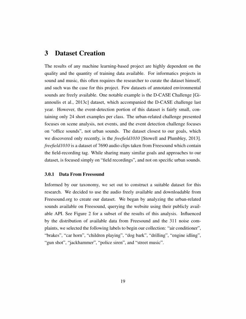
While others have used this folksonomy effectively for things like tag recom-mendation systems to reduce the tag noise [Frederic Font, Joan Serra, 2012], weused this tag data simply to inform our decisions in the creation of our taxonomy.Instead of directly using tags that appear in Freesound to create our taxonomy, wesimply performed a statistical analysis of sounds with search queries related to“city” and “urban” to influence our decisions. A bar graph of the top performingqueries is shown in Figure 2.

2.2.2 Sound Walks

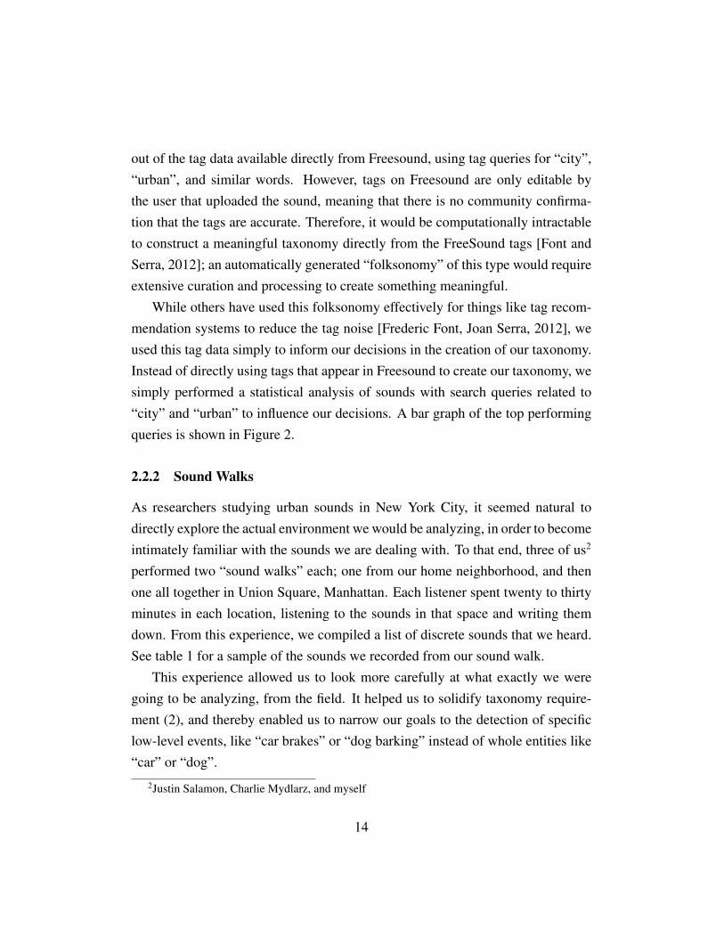
As researchers studying urban sounds in New York City, it seemed natural todirectly explore the actual environment we would be analyzing, in order to becomeintimately familiar with the sounds we are dealing with. To that end, three of us2

performed two “sound walks” each; one from our home neighborhood, and thenone all together in Union Square, Manhattan. Each listener spent twenty to thirtyminutes in each location, listening to the sounds in that space and writing themdown. From this experience, we compiled a list of discrete sounds that we heard.See table 1 for a sample of the sounds we recorded from our sound walk.

This experience allowed us to look more carefully at what exactly we weregoing to be analyzing, from the field. It helped us to solidify taxonomy require-ment (2), and thereby enabled us to narrow our goals to the detection of specificlow-level events, like “car brakes” or “dog barking” instead of whole entities like“car” or “dog”.

2Justin Salamon, Charlie Mydlarz, and myself

14

Table 1: Summary of Sound Walk Sources

Vehicles & Trans-portation

Motorized Vehi-cle sounds

Nature People-related

Car Engine passing Bird DrillTaxi (=car) Engine accel. Squirrel SawBus Engine idling Leaves Conversation/speechTruck Wheels passing Wind Foot stepsBicycle Horn/honk Pigeon Circular sawPolice car (=car) Backing up Dog CoughingFire truck (=truck) Hydraulics SingingAmbient traffic Brakes (screech) LaughingMotorbike Doors opening

(bus - beep)garbage bag (dropping)

Airplane unloading (mech.) Bottle (smashing)Helicopter Bag (rummaging)Metro door alarm Sneeze

BabyCamera (taking pictures)Music (headphones/streetmusicians/car)Leaf blower (engine)Man pushing cart (wheels)Man unlocking store lock

2.2.3 311 Noise Complaints

Our final primary source in determining what sounds to include in our taxonomywas the New York City noise complaints from 311 calls3. We analyzed thesesounds to see which sound complaints occurred most frequently. A full summaryof the noise complaints can be found in Table 2.

3This data is available publicly from https://nycopendata.socrata.com/

15

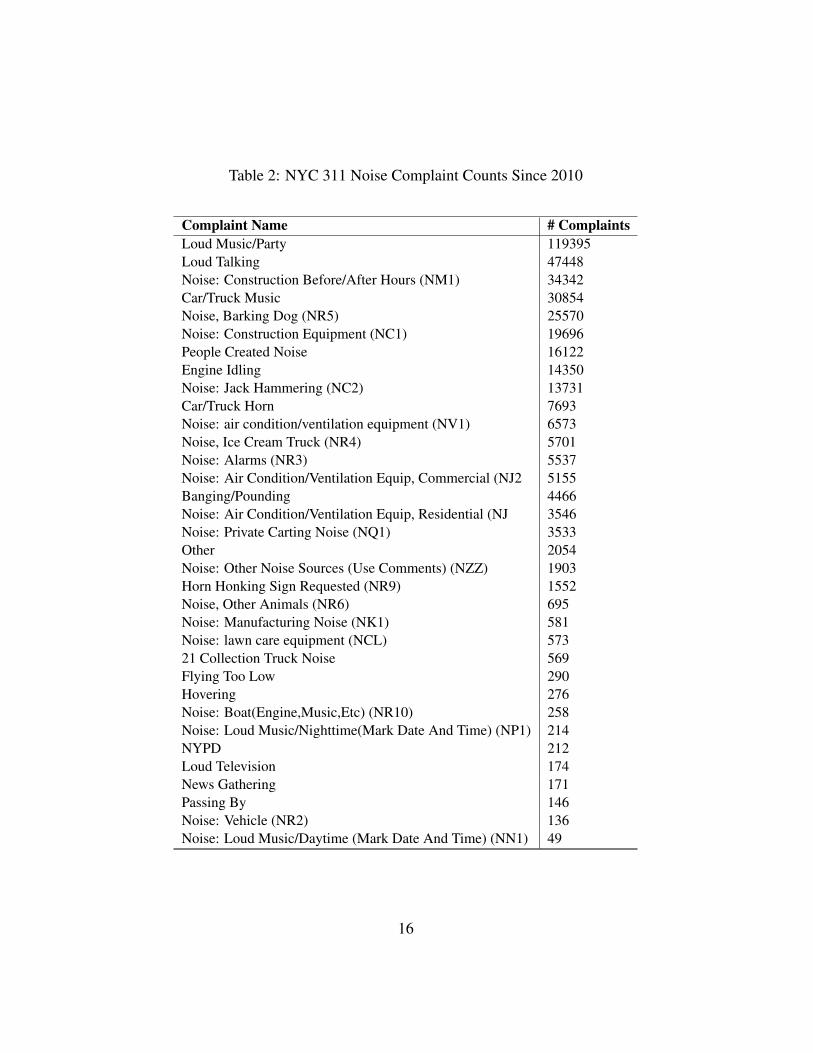
Table 2: NYC 311 Noise Complaint Counts Since 2010

Complaint Name # ComplaintsLoud Music/Party 119395Loud Talking 47448Noise: Construction Before/After Hours (NM1) 34342Car/Truck Music 30854Noise, Barking Dog (NR5) 25570Noise: Construction Equipment (NC1) 19696People Created Noise 16122Engine Idling 14350Noise: Jack Hammering (NC2) 13731Car/Truck Horn 7693Noise: air condition/ventilation equipment (NV1) 6573Noise, Ice Cream Truck (NR4) 5701Noise: Alarms (NR3) 5537Noise: Air Condition/Ventilation Equip, Commercial (NJ2 5155Banging/Pounding 4466Noise: Air Condition/Ventilation Equip, Residential (NJ 3546Noise: Private Carting Noise (NQ1) 3533Other 2054Noise: Other Noise Sources (Use Comments) (NZZ) 1903Horn Honking Sign Requested (NR9) 1552Noise, Other Animals (NR6) 695Noise: Manufacturing Noise (NK1) 581Noise: lawn care equipment (NCL) 57321 Collection Truck Noise 569Flying Too Low 290Hovering 276Noise: Boat(Engine,Music,Etc) (NR10) 258Noise: Loud Music/Nighttime(Mark Date And Time) (NP1) 214NYPD 212Loud Television 174News Gathering 171Passing By 146Noise: Vehicle (NR2) 136Noise: Loud Music/Daytime (Mark Date And Time) (NN1) 49

16

2.3 The Compiled Taxonomy

Finally, we constructed our taxonomy, keeping in mind our requirements and theabove data analysis. Our taxonomy considers only urban sounds, and therefore be-gins at a lower level than some previous environmental taxonomies. In the spirit ofthose previously proposed taxonomies, however, we defined four top-level groups:human, nature, mechanical, and music. To cover our second requirement, theleaves of our taxonomy are designed to be specific and unambiguous. Finally,to relate our taxonomy to urban sounds, we built our taxonomy around semanticdata acquired from Freesound searches, “sound walks”, and common 311 noisecomplaints, as described above. The taxonomy consists of two types of nodes: theboxes with rounded edges represent the hierarchy of conceptual sources that pro-duce sounds, where as the rectangular boxes represent specific describable sounds.While the conceptual sources form a hierarchy, the sound objects represented bythe rectangles have no direct hierarchy, and can be properties of many sources.This allows a variety of “multiple inheritance”, in a way similar to object-orientedprogramming. For instance, police, ambulance, and taxi are all of the class “car”,but only the police and ambulance can produce the sound “siren”, where as alltypes of “road” vehicles share classes for “engine idling”, “brakes screeching”,etc. See final taxonomy in Figure 1.

17

Urb

an A

cous

tic

Envi

ronm

ent

Hum

anN

atur

eM

echa

nica

lM

usic

Voic

eM

ovem

ent

Elem

ents

Anim

als

Plan

ts/

Vege

tatio

nAm

plifi

edN

on-

ampl

ified

Mot

orize

d Tr

ansp

ort

Con

stru

ctio

nVe

ntila

tion

Non

-mot

orize

d Tr

ansp

ort

Soci

al/S

igna

ls

- Spe

ech

- Lau

ghte

r- S

hout

ing

- Cry

ing

- Cou

ghin

g- S

neez

ing

- Sin

ging

- Inf

ant

- Chi

ldre

n

- Foo

tste

ps- W

ind

- Wat

er- T

hund

er

- Dog

{bar

k}- D

og {h

owl}

- Bird

{tw

eet}

- Lea

ves

{rust

ling}

Air

Mar

ine

Rail

Road

- Airp

lane

- Hel

icop

ter

Car

Bus

Truc

kTr

ain

(ove

rgro

und)

Subw

ay(u

nder

grou

nd)

Fire

eng

ine

Mot

orcy

cle

Priv

ate

Taxi

Polic

eAm

bula

nce

Priv

ate

Gar

bage

tru

ckPr

ivat

ePo

lice

- Eng

ine

{idlin

g}- E

ngin

e {p

assi

ng}

- Eng

ine

{acc

eler

atin

g}- H

orn

- Bra

kes

{scr

eech

ing}

- Whe

els

{pas

sing

}

- Pne

umat

ics

- Bac

king

up

{bee

ping

}- R

attli

ng p

arts

Bus

- Sire

n

- Jac

kham

mer

- Ham

mer

ing

- Dril

ling

- Saw

ing

- Exp

losi

on- E

ngin

e {ru

nnin

g}

- Air

cond

ition

erBi

cycl

eSk

ateb

oard

Live

Reco

rded

- Hou

se p

arty

- Clu

b- C

ar ra

dio

- Ice

cre

am tr

uck

- Boo

mbo

x / s

peak

ers

- Whe

els

on tr

acks

- Rum

ble

- Bre

aks

{scr

eech

ing}

- Rec

orde

d an

noun

cem

ents

Boat

- Spo

kes

- Bel

l

- Bel

ls- C

lock

chi

mes

- Ala

rm /

sire

n- F

irew

orks

- Gun

sho

t

- Hyd

raul

ic ra

ms

Figure 1: Urban Sound Taxonomy

3 Dataset Creation

The results of any machine learning-based project are highly dependent on thequality and the quantity of training data available. For informatics projects insound and music, this often requires the researcher to curate the dataset himself,and such was the case for this project. Few datasets of annotated environmentalsounds are freely available. One notable example is the D-CASE Challenge [Gi-annoulis et al., 2013c] dataset, which accompanied the D-CASE challenge lastyear. However, the event-detection portion of this dataset is fairly small, con-taining only 24 short examples per class. The urban-related challenge presentedfocuses on scene analysis, not events, and the event detection challenge focuseson “office sounds”, not urban sounds. The dataset closest to our goals, whichwe discovered only recently, is the freefield1010 [Stowell and Plumbley, 2013].freefield1010 is a dataset of 7690 audio clips taken from Freesound which containthe field-recording tag. While sharing many similar goals and approaches to ourdataset, is focused simply on “field recordings”, and not on specific urban sounds.

3.0.1 Data From Freesound

Informed by our taxonomy, we set out to construct a suitable dataset for thisresearch. We decided to use the audio freely available and downloadable fromFreesound.org to create our dataset. We began by analyzing the urban-relatedsounds available on Freesound, querying the website using their publicly avail-able API. See Figure 2 for a subset of the results of this analysis. Influencedby the distribution of available data from Freesound and the 311 noise com-plaints, we selected the following labels to begin our collection: “air conditioner”,“brakes”, “car horn”, “children playing”, “dog bark”, “drilling”, “engine idling”,“gun shot”, “jackhammer”, “police siren”, and “street music”.

19

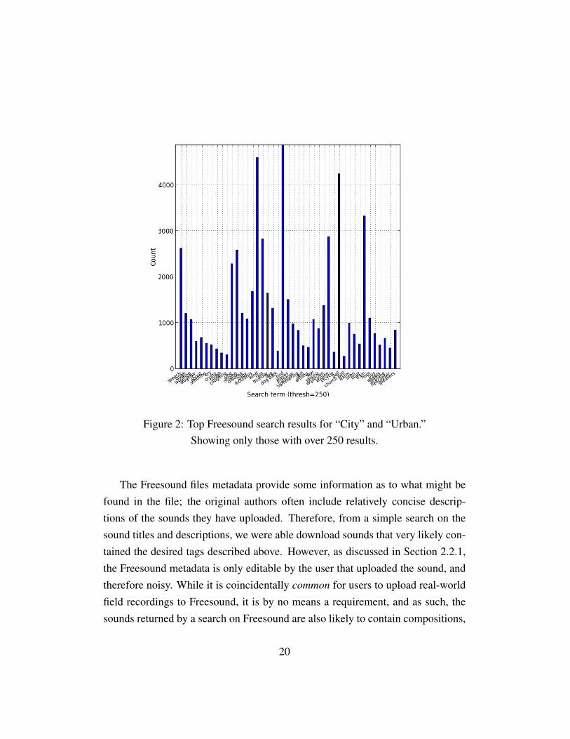
Figure 2: Top Freesound search results for “City” and “Urban.”Showing only those with over 250 results.

The Freesound files metadata provide some information as to what might befound in the file; the original authors often include relatively concise descrip-tions of the sounds they have uploaded. Therefore, from a simple search on thesound titles and descriptions, we were able download sounds that very likely con-tained the desired tags described above. However, as discussed in Section 2.2.1,the Freesound metadata is only editable by the user that uploaded the sound, andtherefore noisy. While it is coincidentally common for users to upload real-worldfield recordings to Freesound, it is by no means a requirement, and as such, thesounds returned by a search on Freesound are also likely to contain compositions,

20

Search Tag # Original Files # Accepted Files # FG Segs. # BG Segs. Total Seg. Dur.(mins)

air conditioner 128 64 47 18 85.67car horn 188 129 105 150 12.26

children playing 296 158 108 59 285.2dog bark 599 388 558 356 153.94drilling 460 119 360 29 205.85

engine idling 162 98 155 11 47.78gun shot 516 121 304 58 9.94

jackhammer 64 45 348 63 52.28police siren 132 77 45 73 35.05street music 272 167 116 84 364.05

Total 2,817 1,316 2,146 901 1,252

Figure 3: Raw Data Summary

synthesized sounds, and other undesirable sounds. To prepare a dataset for re-search, three steps were required: 1) selecting the files that indeed contained thesounds desired; 2) annotating each file with the location of the desired sound; and3) preparation of the sound files into a form ready for research. Each of step ofthe dataset curation process is described in more detail below. A block diagramof the dataset curation process is shown in Figure 4.

3.0.2 Phase 0: Download & Collect Raw Data

The first step in creating our data was to download all of the sounds with metadatacontaining the desired tags to a single folder. We wrote a Python script to querythe FreesoundAPI, process, and organize the results. A summary of the originalraw data is shown in Figure 3.

3.0.3 Phase 1: Select the Files

Next, in order to be sure that we were only working with files that indeed con-tained the sound in question, we listened to each and every file to check for thepresence of the sound in the file. Since the more detailed work is done in Phase 2,

21

all we needed to do for this phase was to determine that the sound occurred any-where in the file. We then moved the file to a folder for “accepted” or “rejected”.

3.0.4 Phase 2: Annotate the Files

Figure 4: Dataset Creation Process

In Phase 2, we annotated the active regionof each sound in each file for each class,hereafter the “activations”. To do this, weused the popular open source software Au-dacity4, which includes a utility for “label”tracks. Audacity’s label tracks allow anno-tations of arbitrarily named labels, simplyby dragging over a region and typing on thekeyboard. The user can then simply exportthe label tracks to text files, where each an-notation represented by a single line con-taining start time, end time, and the labelgiven.

During the process, we decided to labeleach sound with a saliency measure of ‘1’,‘2’, or ‘3’ A ‘1’ indicates “foreground”,where the sound is not masked by any sig-nificant noise or other sounds. A ‘2’ in-dicates “background”, or that the sound ismasked by noise or other sounds. A ‘3’ in-dicates “distant”, or that the sound is quite difficult for even the annotator to hearwithout filtering or turning the sound up.

The process is roughly as follows for each track:

• Open track in spectrogram view Audacity.

4http://audacity.sourceforge.net/

22

• Create a label track.

• Listen to the recording, marking each occurrence of the sound with thesaliency label. If sounds occur close together, mark them all as one.

A summary of the data created from phase 2 can be seen in Figure ??.In the annotation phase, we decided due to the sonic differences in train brakes

and other brakes sounds to split the brakes class into “train brakes” and “roadbrakes” classes. Following the completion of Phase 2, we decided to discardboth of our “brakes” classes, because the “road brakes” had far too few segmentscompared to all of the other classes, and “train brakes” did not fit thematicallywith the rest of our classes, which are all sounds that would be found outside inthe urban environment. Removing these two classes left us with an even 10 classesfor the final dataset.

3.0.5 Phase 3: Prepare a Canonical Dataset

The final stage in the creation of our dataset required us to prepare a canonicalversion of the dataset for research. This process involved two stages: splitting theannotated segments up into short slices, and then allocating them to folders forcross-validation. To split the segments up into slices, we had to determine twoparameters: the slice duration and the hop size.

To determine the slice duration, we first had to determine what length splitswere going to be adequate to detect any particular class in our dataset. Our goalin determining the slice duration was to have the shortest possible slices whilewhile maintaining the maximum recognition rate. We began by performing a briefperceptual experiment, whereby we split the segments into slices of 1 second, 2seconds, and 3 seconds, and listened to a random sampling to determine whichclasses we could personally identify in that amount of time. We discovered thatfor most of our classes, 2 seconds would be enough. However, for some classes,it was easy to mistake one for the other in a blind test; for instance, given a par-ticular sample “street music” with an electric guitar playing a chord for only two

23

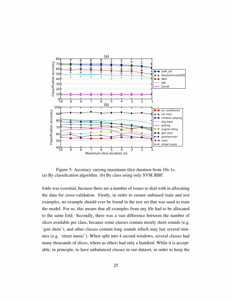
seconds, it was difficult to distinguish if it was a guitar, or train brakes. At threeseconds, there was enough context provided that we did not have any difficultiesof this sort. A similar but more rigorous perceptual study compared listener ac-curacy and confidence of recognition to slices of 2, 4, and 6 seconds [Chu et al.,2008]. The study determined that listener recognition rate increases significantlyfrom 2 to 4 seconds, but with only a slight increase from 4 to 6 seconds. Their al-gorithm had a similar recognition rate at 4 seconds to the listener recognition rate.We also performed an experiment with slice duration where we varied the sliceduration from 1 second to 10 seconds in 1 second intervals, and re-ran our base-line system (described in Section ?? for each. The results of this experiment areshown in Figure 5. These results show a general decrease in overall recognitionrate below 6 seconds, however, the rates when looking at individual classes is farmore complex. Ultimately, we chose 4 seconds, based on our stated requirementto have the shortest possible slices; the study in [Chu et al., 2008] shows adequaterecognition at 4 seconds, and in our experiment, 4 seconds is the last point beforethe overall recognition rate begins to drop off more drastically.

For short sounds, such as “gun shots” and “dog barks”, the majority of therelevant sound tends to be contained within the first 4 seconds of a segment, andsegments tend to be 4 seconds or shorter in length. However, segments longer thanfour seconds will either contain multiple occurrences of short sounds, or a morecontinuous sound, such as “air conditioner” or “children playing”. Therefore, weselected a 50% hop size for our slices, or 2 seconds. If the original segment is lessthan 4 seconds long, we keep the entire segment; slices generated which are lessthan 4 seconds from a file which is greater than 4 seconds long are discarded. Forinstance, a segment which is seven segments long will generate two slices: onefrom 0-4 seconds, and one from 2-6 seconds. The remaining one second will bediscarded. This is intended to provide robustness to time shifts of sources whichoccur multiple times within a segment.

Machine learning datasets are commonly organized into “folds”, to facilitate10-fold cross validation. In the case of our dataset, releasing it already split into

24

10 9 8 7 6 5 4 3 2 10

10

20

30

40

50

60

70

80

Cla

ssific

ati

on a

ccura

cy(a)

SVM_rbf

RandomForest500

IBk5

J48

ZeroR

10 9 8 7 6 5 4 3 2 1Maximum slice duration (s)

40

50

60

70

80

90

100

Cla

ssific

ati

on a

ccura

cy

(b)

air conditioner

car horn

children playing

dog bark

drilling

engine idling

gun shot

jackhammer

siren

street music

Figure 5: Accuracy varying maximum slice duration from 10s-1s.(a) By classification algorithm. (b) By class using only SVM RBF.

folds was essential, because there are a number of issues to deal with in allocatingthe data for cross-validation. Firstly, in order to ensure unbiased train and testexamples, no example should ever be found in the test set that was used to trainthe model. For us, this means that all examples from any file had to be allocatedto the same fold. Secondly, there was a vast difference between the number ofslices available per class, because some classes contain mostly short sounds (e.g.‘gun shots’), and other classes contain long sounds which may last several min-utes (e.g. ‘street music’). When split into 4 second windows, several classes hadmany thousands of slices, where as others had only a hundred. While it is accept-able, in principle, to have unbalanced classes in our dataset, in order to keep the

25

distribution between classes within a reasonable margin, we were restricted thenumber of slices from certain classes to 1000 across all folds.The fold allocation algorithm is summarized as follows:

for all class labels dofor all folds do

Assign a file from the class to that fold.end forfor all folds, until out of slices or (total slices ≥ 1000) do

Copy randomly chosen slice from a file assigned to that fold into the foldfolder

end forend for

3.0.6 Final Dataset Statistics

The final UrbanSound dataset contains 10 low-level classes from the taxonomy:air conditioner, car horn, children playing, dog bark, drilling, engine idling, gunshot, jackhammer, siren, and street music. The complete dataset contains a totalof 3075 labeled occurrences, for a total of 18.5 hours of audio. The distributionof total occurrence duration per class and per salience is displayed graphically inFigure 6(a).

The collection of 1314 full-length recordings, with corresponding annotationfiles and Freesound metadata files are all provided with the base UrbanSound

dataset, and will be available for download online. For research on urban sourceclassification, our “canonical” dataset, the UrbanSound8K, containing 4s slices ofannotations of the original file, will also be available online. The canonical versioncontains a total of 8732 slices for 8.75 hours of recordings, split up into 10 folds.The distribution of slices per class in UrbanSound8k is shown in Figure 6(b).

26

stree child dog b air c drill jackh engin siren car h gun s0

50

100

150

200

250

300

350

400

Tota

l dura

tion (

min

ute

s)

(a)

FG

BG

stree child dog b air c drill jackh engin siren car h gun s0

200

400

600

800

1000

Slic

es

(b)

FG

BG

Figure 6: Occurrence Duration Per Class(a) Total occurrence duration per class in UrbanSound. (b) Slices per class inUrbanSound8k. Breakdown by foreground (FG) / background (BG).

27

Figure 7: Baseline Block Diagram

4 Baseline System

4.1 System Overview

With dataset in hand, our first task was to create a baseline set of classificationexperiments to compare our results with. The goal of the baseline experimentswas not to produce optimal parameters and to maximize accuracy, but to studythe problems and characteristics of the dataset itself using off-the-shelf tools. Theblock diagram of the baseline system can be seen in Figure 7. It is composed oftwo simple parts: the Time Frequency Representation (MFCCs), and classifica-tion.

We used MFCCs for our baseline time-frequency representation, because theyobtain competitive results in many other timbre-based classification systems, andhave been used successfully in environmental sound analysis, such as [Chaudhuriand Raj, 2013]. See Section 5.1 for a further look at using MFCCs for audioclassification systems. We extracted all features on a per-frame basis using awindow size of 23.2ms and 50% frame overlap. Our baseline MFCC featureswere computed with 40 Mel bands between 0 and 22050 Hz, and we kept thefirst 25 MFCC coefficients. No pre-emphasis nor liftering was applied. Afterfeature extraction, the values for each frame are summarized across the slice, usingthe following summary statistics: minimum, maximum, median, mean, variance,skewness, kurtosis, and the mean and variance of the first and second derivatives.This resulted in a feature vector with 255 dimensions for each slice. We used

28

Essentia 5 to calculate the MFCCs and create the summary statistics across all theframes in an audio file.

We used the Weka6 data mining software to experiment with various classifica-tion algorithms. Every experiment is run with 10-fold cross validation, and in eachfold, Weka’s built in correlation based feature selection is used to select attributesand avoid overfitting. We use the default parameters for each algorithm. Classifi-cation algorithms included the support vector machine with radial basis functionand polynomial kernels, random forests, decision tree, and k-nearest neighbors.

We performed several experiments using our baseline classification architec-ture prior to the creation of our canonical dataset, in order to minimize the effectof parameters of dataset creation on classification accuracy. We tested the MFCCparameters to see how the number of Mel bands and the number of coefficientseffected our baseline results. We tested the duration of our slices in the creationof our dataset, to evaluate how slice length effects classification accuracy. Finally,for the parameters determined in these experiments, we present the final classi-fication results per class, examine the confusion matrices produced, and analyzethe results.

Before settling on the final MFCC parameters for the baseline, we ran an ex-periment which evaluated the change in classification accuracy based on the num-ber of Mel bands used in the computation of the Mel spectrum, as shown in Fig-ure 8. Plot (a) shows the best overall accuracy over all classification algorithms tobe the Radial Basis Function (RBF) kernel Support Vector Machine to be between30 and 40 bands, with another rise at 80 bands. Looking at the classification accu-racy across the individual classes in our dataset for just the SVM with RBF kernel(b), we see a relatively flat distribution for some sounds, and a drastic change insome other classes. Car horn is the notable example, where classification accu-racy drastically increases with the increase in bands from 10 to 50; this makessense for a very tonal sound, such as the car horn, as the resolution of discernible

5http://essentia.upf.edu/6http://www.cs.waikato.ac.nz/ml/weka/

29

10 20 30 40 50 60 70 800

10

20

30

40

50

60

70

80C

lass

ific

ati

on a

ccura

cy(a)

SVM_rbf

RandomForest500

IBk5

J48

ZeroR

10 20 30 40 50 60 70 80Number of mel bands / MFCC coefficients

40

50

60

70

80

90

100

Cla

ssific

ati

on a

ccura

cy

(b)

air conditioner

car horn

children playing

dog bark

drilling

engine idling

gun shot

jackhammer

siren

street music

Figure 8: Accuracy over varying number of Mel filters.

frequencies increases with the number of available Mel bands. We also see thatthe “siren” sound, which is also tonal in character, starts relatively high at near75%, and gradually decreases with increasing Mel bands. Since most classes startto decrease after 40 bands, we choose to use 40 bands for further experiments.

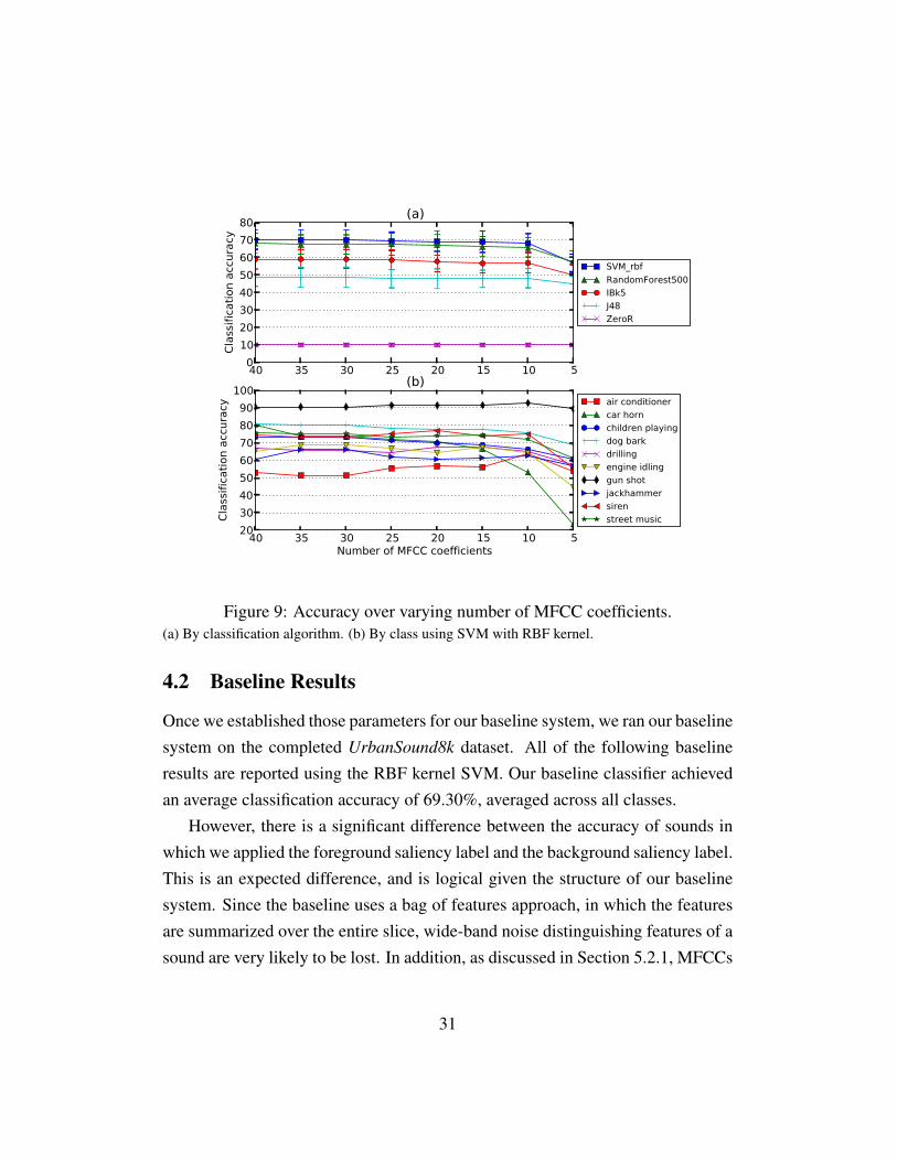
We performed a similar experiment looking at the number of MFCC coef-ficients Figure 9. This experiment produced significantly more obvious results;the overall classification results were relatively flat across all runs, although thein-class results have some minor oscillation. With 10 coefficients and under, re-sults drop drastically. We chose 25 coefficients for our experiments, in order tomaximize classification accuracy while minimizing dimensionality.

30

40 35 30 25 20 15 10 50

10

20

30

40

50

60

70

80C

lass

ific

ati

on a

ccura

cy(a)

SVM_rbf

RandomForest500

IBk5

J48

ZeroR

40 35 30 25 20 15 10 5Number of MFCC coefficients

20

30

40

50

60

70

80

90

100

Cla

ssific

ati

on a

ccura

cy

(b)

air conditioner

car horn

children playing

dog bark

drilling

engine idling

gun shot

jackhammer

siren

street music

Figure 9: Accuracy over varying number of MFCC coefficients.(a) By classification algorithm. (b) By class using SVM with RBF kernel.

4.2 Baseline Results

Once we established those parameters for our baseline system, we ran our baselinesystem on the completed UrbanSound8k dataset. All of the following baselineresults are reported using the RBF kernel SVM. Our baseline classifier achievedan average classification accuracy of 69.30%, averaged across all classes.

However, there is a significant difference between the accuracy of sounds inwhich we applied the foreground saliency label and the background saliency label.This is an expected difference, and is logical given the structure of our baselinesystem. Since the baseline uses a bag of features approach, in which the featuresare summarized over the entire slice, wide-band noise distinguishing features of asound are very likely to be lost. In addition, as discussed in Section 5.2.1, MFCCs

31

air c car h child dog b drill engin gun s jackh siren stree All 0

20

40

60

80

100C

lass

ific

ati

on a

ccura

cy

Both

FG

BG

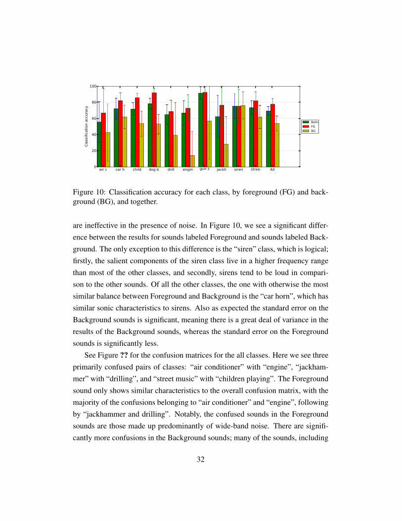
Figure 10: Classification accuracy for each class, by foreground (FG) and back-ground (BG), and together.

are ineffective in the presence of noise. In Figure 10, we see a significant differ-ence between the results for sounds labeled Foreground and sounds labeled Back-ground. The only exception to this difference is the “siren” class, which is logical;firstly, the salient components of the siren class live in a higher frequency rangethan most of the other classes, and secondly, sirens tend to be loud in compari-son to the other sounds. Of all the other classes, the one with otherwise the mostsimilar balance between Foreground and Background is the “car horn”, which hassimilar sonic characteristics to sirens. Also as expected the standard error on theBackground sounds is significant, meaning there is a great deal of variance in theresults of the Background sounds, whereas the standard error on the Foregroundsounds is significantly less.

See Figure ?? for the confusion matrices for the all classes. Here we see threeprimarily confused pairs of classes: “air conditioner” with “engine”, “jackham-mer” with “drilling”, and “street music” with “children playing”. The Foregroundsound only shows similar characteristics to the overall confusion matrix, with themajority of the confusions belonging to “air conditioner” and “engine”, followingby “jackhammer and drilling”. Notably, the confused sounds in the Foregroundsounds are those made up predominantly of wide-band noise. There are signifi-cantly more confusions in the Background sounds; many of the sounds, including

32

all of those from the complete and Foreground confusions, had as many or moreconfusions as they had correct results. See Figure ?? for the foreground and back-ground sound confusion matrix.

33

AI CA CH DO DR EN GU JA SI ST

AI

CA

CH

DO

DR

EN

GU

JA

SI

ST

555 4 77 63 54 131 0 33 7 76

25 304 14 19 26 9 1 8 3 20

38 3 715 54 27 16 0 4 28 115

33 12 82 783 15 5 3 1 29 37

51 43 24 50 646 20 5 110 31 20

130 12 23 40 27 662 0 84 13 9

0 7 0 19 2 0 343 3 0 0

70 20 2 1 147 72 0 597 51 40

23 13 72 40 24 17 0 3 712 25

35 15 119 23 16 12 1 14 32 733

(a) All slices.

AI CA CH DO DR EN GU JA SI ST

AI

CA

CH

DO

DR

EN

GU

JA

SI

ST

388 4 0 5 31 110 0 20 7 4

0 129 1 13 4 0 1 1 1 3

3 0 501 36 0 1 0 1 13 33

2 3 21 592 3 0 2 0 7 15

36 40 15 47 614 19 5 93 16 17

90 7 12 38 27 653 0 84 4 1

0 4 0 12 2 0 283 3 0 0

20 17 1 1 84 40 0 542 0 26

0 9 13 22 16 0 0 0 206 3

6 6 36 16 9 6 1 11 26 508

(b) Foreground slices only.

AI CA CH DO DR EN GU JA SI ST

AI

CA

CH

DO

DR

EN

GU

JA

SI

ST

167 0 77 58 23 21 0 13 0 72

25 175 13 6 22 9 0 7 2 17

35 3 214 18 27 15 0 3 15 82

31 9 61 191 12 5 1 1 22 22

15 3 9 3 32 1 0 17 15 3

40 5 11 2 0 9 0 0 9 8

0 3 0 7 0 0 60 0 0 0

50 3 1 0 63 32 0 55 51 14

23 4 59 18 8 17 0 3 506 22

29 9 83 7 7 6 0 3 6 225

(c) Background slices only.

Figure 11: Baseline Confusion Matrices (SVM classifier with RBF kernel.)

5 Feature Learning System

In this section, we present our exploration of feature learning techniques as amethod to improve the baseline results. We begin with a history of environmen-tal sound classification and the components of the sound classification pipeline.Finally, we present the results of our feature learning module, and analyze theresults in the context of the baseline.

5.1 Background

Analysis of environmental sound, and in particular the automatic source-basedidentification of events in urban recordings, is still a relatively new field. Onlyin the recently have significant efforts been made towards this goal. Research inautomatic identification of environmental sounds is far more sparse than in theanalysis of scenes. In this section we look at previous work in the related fields ofsource identification and acoustic event identification.

One significant landmark in the computational acoustic scene and event anal-ysis was the creation of the IEEE AASP D-CASE challenge for ComputationalAuditory Scene Analysis, an international challenge with a public evaluation withthe goal of advancing the state of the art in the areas of modeling acoustic scenesand detecting audio events [Giannoulis et al., 2013a]. There are several similarchallenges, such as the MIREX competition, that have existed in related fields,but this is the first such challenge focusing on detection and classification ofnon-speech and non-music signals. This competition, presented by the QueenMary University of London, consisted of three challenges: the first is a scene-analysis challenge, the second is an event-detection challenge, consisting of sep-arate monophonic (non-overlapping sounds), and the third is a event-detectionchallenge consisting of polyphonic (overlapping sounds) components. This com-petition is an exciting development in the field of computational auditory sceneanalysis, creating opportunities for researchers across the world to compare theirresults in a rigorous way. However, the datasets used in the challenge were of

35

a relatively small scale, which makes using them for machine learning researchsomewhat challenging, as the results of machine learning algorithms are directlytied to the size of the training data. In addition, only the scene classificationdataset made use of urban sounds; the event detection datasets were made up al-most entirely of “office” sounds, making it of limited use for our research.

However, this challenge does provide a useful way to look at the sorts of algo-rithms that researchers are using for event detection problems. For the scene clas-sification task, the baseline used MFCCs for features, and used a bag-of-framesapproach in classification. MFCCs, or some variation on them, were by far themost common features used in the 2013 evaluation of the challenge, and supportvector machines were the most common classifier. To make a decision across theentire recording, majority voting and max-pooling techniques were common. Forthe event detection challenge, non-negative matrix factorization was the baselineapproach, and made a significant appearance in the challenge entries. MFCCswere also used in a significant portion of the entries in this category. The resultsof the D-CASE challenge are presented in [Giannoulis et al., 2013b].

Several recent approaches to machine hearing of environmental sounds takedifferent directions than the standard ones discussed above. One approach to envi-ronmental scene recognition is presented in [Chu et al., 2008] Chu et al. proposeda method using Matching Pursuits (MP) to learn a dictionary of atoms for featureselection, combined with MFCC’s. This article stands out above many of the restwe looked at. It was the only one we came across in our research that made sig-nificant use of time-domain features. Chu et al. state plainly many of the failingsof MFCCs. Their MP-based features not only perform well in noisy urban envi-ronments, but they also perform significantly better than MFCC’s in those cases.The MP-based features combine with MFCCs to yield an even better result.

Another approach is to use image processing techniques on the spectrogram.An example of this is found in [Dennis, 2011], where Dennis uses presents two im-age processing methods, the “Spectrogram Image Feature”, and “Subband PowerDistribution Image Feature”, in combination with a variety of k-Nearest Neighbor,

36

to yield very good results over his baseline system. Even in the presence of noise,particular sounds in the spectrum typically have a characteristic shape which isrecognizable to the human eye. This computer vision approach therefore has thenotable feature of being relatively robust to noisy environments, by recognizingthe characteristic shape of a sound in a spectrogram.

Several approaches to event and scene classification attempt to invent new timefrequency representations. Richard Lyon proposes one perceptually motivatedapproach using a pole-zero filter cascade (PZFC) which simulates the impedancebehavior of the basilar membrane [Lyon, 2010]. Lyon’s approach is designedfrom end to end to simulate the human hearing system, and is drastically differentfrom other systems proposed to date. Lyon’s system combines the PZFC witha sparse-coding feature extraction, and his experimental results show significantimprovement over features learned on MFCCs.

Detection of sounds in an acoustic environment requires knowledge of vari-ous time resolutions, as in many cases the difference between two sources is onlyidentifiable by observing the sound over time. For instance, the difference be-tween the sound of a screeching car breaks (a short, high pitched sound), and apolice siren (a long high pitched sound that changes frequency slowly) may onlybe detectable if the sound is observed over a longer time widow. Dieleman usesthree different approaches to solve this problem in [Dieleman and Schrauwen,2013]; multi-resolution spectrograms, and the Gaussian and Laplacian pyramid.Dieleman found no clearly winner architecture among these, but found that dif-ferent architectures tended to work better for different classes or different tasks,based on how time-dependent the signal is. Another multiresolution algorithm ispresented in [Lallemand et al., 2012], which presents wavelet-based features, anda similarity measure for those features using Kullback-Leibler divergence. Thisapproach gets improved results over MFCCs with Euclidean distance for an envi-ronmental sound recognition task, however, their system only looks at pair-wisesimilarity for evaluation results, and is therefore difficult to compare with the typeof classification systems we are interested in.

37

In some cases, the Gaver taxonomy has been used directly in conjunction withaudio analysis to perform sound classification. In machine learning research somework has recently been done using joint embedding spaces [Weston et al., 2010],where a mapping is learned from the audio to a semantic space which is simulta-neously the tag space. This allows the machine to infer a tag which exists in thetag space from an audio example which was never labeled. Roma et. al performa similar experiment using the Gaver taxonomy, with an expanded search spacewidened using the Wordnet [Miller, 1995] database in combination with audiofrom Freesound [Roma et al., 2010].

For a deeper look into the state of classification and automatic tagging in re-lated audio fields, see [Bertin-Mahieux et al., 2010]

5.2 Analysis Pipeline

The results of any computational classification algorithm, such as the one dis-cussed here, are highly dependent on the quality of the input. In machine learningterminology, the input representation into a classifier is typically referred to asthe “features”. Traditionally, in machine hearing research communities, featureshave often been hand engineered using extensive domain knowledge [Humphreyet al., 2012]. For example, a knowledge of music theory allows one to create rulesor heuristics on how to analyze a musical recording that can be encoded into analgorithm for analysis. At the other end of the feature spectrum from feature engi-neering is feature learning. This involves the use of machine learning techniquesto “learn” the features from the low-level input to the system. In the followingsection, we discuss approaches to both of these techniques that have been usedthroughout the literature, and the benefits to both.

5.2.1 Engineered Features

The most common features used in audio classification of any type are MFCCs, orMel-Frequency Cepstral Coefficients. MFCCs were designed initially for speech

38

Figure 12: Feature EngineeringPipeline

In the feature engineering approach, rawaudio is converted into an engineered, or

human-designed time-frequencyrepresentation, which is fed directly into

the classifier.

Figure 13: Feature Learning PipelineIn the feature learning approach, a simpletime-frequency representation is used, anda model (sometimes called a dictionary) islearned automatically by example from thedata. Features are then created by taking

the dot product of the input with the model.

39

detection and classification in the late 1990s, and have proven to be very success-ful for classifying phonemes in speech signals. The success of MFCCs in thespeech processing community eventually interested those in the music and soundinformatics communities, and MFCCs have since grown to be the de facto stan-dard for timbral features. MFCCs are a relatively low-dimensional representationof timbre which encodes the spectral envelope of the signal in a small numberof coefficients. They are computed by computing the Discrete Cosine Transform(DCT) on log of the Mel-filtered spectrogram.

It is precisely the low dimensionality that makes MFCCs especially efficient;machine learning classifiers have a tendency to overfit the data if the dimensional-ity of the input representation is too high. MFCCs convert a Fourier input of 1024or 2048 coefficients to one of 13 to 25 coefficients, but maintain a significantamount of important timbral information required to discriminate sounds. This isan efficient coding, in that the coefficients generated are decorrellated from eachother, which makes MFCCs a quality input into a classifier without needing toperform additional PCA. In addition, MFCCs represent the spectral envelope ofa signal, and are therefore essentially transposition invariant. For speech signalsespecially, MFCCs tend to perform very well in classification tasks, but they havealso had good results in instrument classification tasks.

While MFCCs have significant benefits, they are far from perfect. Firstly,they convey information about the static current state of a signal only, whereasall sounds are dynamic in time, having, for instance, a different timbre at thestart of the sound from the middle or end of the sound. Secondly, the perfor-mance of MFCCs are known to degrade significantly in the presence of noise, andare similarly ineffective at representing signals noise-like signals with a relativelyflat spectrum. This problem is especially notable for detecting sounds in urbansoundscapes; unlike music, which is typically recorded in a controlled environ-ment, nearly every signal involved in the classification process is likely to havesome significant noise involved in the signal. Many of the classes of sounds weare interested in urban environments are exactly that sort of noise-like sounds–air

40

conditioners, engines, etc.Several approaches have been presented which try to solve MFCCs’ deficien-

cies by engineering more robust alternatives. One approach, entitled gammatonefrequency cepstral coefficients (GFCCs), suggests a variant of the MFCC rep-resentation using the cubic root of the time frequency representation instead ofthe log, in combination with a gammatone weighted filter bank instead of a Melweighted filter bank. [Zhao and Wang, 2013] Zhao and Wang demonstrate thesemodifications to create robustness of the representation to noise in the signal.

Now that we have established MFCCs as the most common features for tim-bral classification tasks, we take a step back to look at the Mel spectrum, the firststep in the creation of MFCCs. It is calculated by applying a Mel-frequency scalefilterbank on the Fourier spectrum. The Mel scale is a logarithmic scale weightedto coincide approximately with human hearing. The Mel spectrum is a commoninput representation for machine hearing systems. Machine hearing approacheswhich desire a representation closer to the original spectrum, but still reducedin dimensionality, typically use this representation, or a similar one such as theConstant-Q Transform.

The Mel spectrum is particularly useful in machine learning tasks, because itis stable to deformation using a Euclidean norm, unlike the spectrogram [Andenand Mallat, 2012]. However, the averaging used to create The Mel spectrumcauses significant loss of high-frequency information unless the window size iskept small. Several approaches have been created to deal with this problem. Onenotable approach is the use of “scattering coefficients”, which extend The Melspectrum using a cascade of wavelet decompositions and modulus operators to re-cover high frequency resolution while keeping stability to the deformation. Thisscattering representation successfully captures an improved timbral representationcompared to The Mel spectrum. The authors present an extension of this similarto MFCCs in [Mallat et al., 2013], called “deep scattering spectrum”, which getsstate of the art classification results on genre and phoneme classification. The deepscattering spectrum is “deep” in the hierarchical sense, because of the cascade of

41

operations; it’s complexity is engineered, not learned, as in other deep systemsdescribed in the next section.

5.2.2 Learned Features

Feature learning has recently become popular for finding solutions to signal clas-sification problems. A feature learning system “learns” a function of the databy training it on the data itself. Feature learning algorithms are data-driven, anddepend directly on the quality and quantity of the data provided in the learningstage.

Neural networks, in particular “deep networks”, are one of the primary toolsfor feature learning. A neural network is a complex hierarchy of linear and non-linear nodes which can learn complex functions automatically given enough in-put data. “Deep networks” are many-layered versions of neural networks, andthe “deep”-ness of them allows them to learn hierarchies of features, enablingthem to automatically learn very high level features about a signal. Neural net-works were invented as early as the 1940s, and were researched extensively untilthe early 1990s, when successes in other machine learning algorithms eventuallytook the focus in the machine learning community. However, in the last decadeor so, important advancements in training deep networks, combined with the gen-eral increased computing power available in society have brought neural networksback to prominence. Across computational research genres, but specifically in theimage and speech detection communities, deep neural nets have recently beenoutperforming state-of-the-art systems where heuristics-based systems had previ-ously dominated [Krizhevsky et al., 2012].

One of the biggest problems with deep neural networks is that the derivativesthat are backpropagated during supervised training become extremely weak soas to be of minimal effectiveness by the time they reach the beginning of thenetwork. In particular, it was shown that the use of greedy layer-wise training iswhat brought the neural network back to prominence [Hinton et al., 2006]. Thisinitializes the data in an unsupervised fashion, one layer at a time, while freezing

42

the weights of the other layers. An unsupervised algorithm such as k-means orsparse coding is typically used for this. Unsupervised initialization of the networksignificantly improves the performance of neural networks.

One specific variant on this approach is the use of spherical k-Means to ini-tialize feature learning layers, as described by Coates and Ng in [Coates and Ng,2012]. Spherical k-Means is a slight variation on the traditional k-Means algo-rithm, where the centroids are constrained to the unit sphere at each update step.This has the function of using the cosine distance for similarity to points in theinput space instead of the Euclidean distance, which is typically used in tradi-tional k-Means. Coates and Ng also specify that the effectiveness of the learnedcentroids is significantly improved by the addition of ZCA7 whitening, which“sphere’s” the data, allowing the unit sphere-constrained centroids to maximallyrepresent the data.

Coates and Ng describe the use of spherical k-means in image detection,but the algorithm is equally as effective in processing audio. One approach byDieleman uses spherical k-means in combination with multiscale approaches inan audio tag prediction and a similarity metric learning task to [Dieleman andSchrauwen, 2013]. Unlike the Coates and Ng design, Dieleman uses PCA whiten-ing instead of ZCA whitening, which serves to further decorellate the inputs fromeach other. This step can significantly help the quality of the input representation,and serves to decorellate the input representation. See [Nam et al., 2012, Hamelet al., 2012] for further examples of PCA whitening used with audio.

To compare the quality of dictionaries learned using the data, we can also lookat dictionaries composed of noise. [Lutfi et al., 2009] uses a dictionary composedof random bases, with no learning, and has competitive results, in a process knownas “compressed sensing.” The representation allows accurate compression of thesignal using a small dictionary. This algorithm significantly reduces computa-tion time over a learned representation, as no knowledge of the data is necessarybeforehand, other than the dimensionality of the desired bases.

7Zero-Phase Component Analysis

43

While feature learning is especially effective in deep architectures, it has alsobeen proven to be effective in shallow architectures [Coates et al., 2011]. To beginwith a feature learning architecture which is easily comparable with our baselinesystem, we present in this thesis a system which is loosely related to Dieleman’ssystem, using a single feature learning layer trained using spherical k-means onPCA whitened audio data.

5.2.3 Classification

After the choice of features, the next component in a classification system is theclassifier itself. At a very basic level, a classifier simply takes an input and as-signs one or more “labels” or “classes” to that input. The classifier is trained or“learned” from the data itself, and as a result the quality of the results depends en-tirely on the data the classifier was trained on. In this project, we use the Weka datamining software to perform our classification. While the classifier is an importantcomponent of the automatic classification system, the focus in this research is onthe features input into the classifier, not the classifier itself. Therefore, after ex-perimenting with different classifiers in our baseline system, we settle on usingonly the Support Vector Machine with a Radial Basis Function kernel as our clas-sifier. With that in mind, we briefly take a look at how features are passed into theclassifier.

Events in audio recordings are composed of a sequence of frames, but framesgenerated from windowed spectrograms are typically on the order of 25 to 50milliseconds, which is much shorter than the duration of most events of interest. Inorder to classify individual events, a decision has to be aggregated across severalframes. One technique for classifying a section of audio is called the “bag offrames” approach. Instead of analyzing each frame of a signal to determine whichclass or classes it might belong to, and then summarizing the frame-level results,bag of frames takes summary statistics across an entire input sound, be it a track ora segment of a track. For instance, with MFCCs, the final features that were usedin the classifier would be the mean, variance, mean and variance of the first and

44

second derivatives, minimum, maximum, etc., each across all of the samples inthe frame. Even though this approach looses a significant amount of information,it turns out to perform quite well on certain tasks, such as scene identification.Other approaches include passing the individual frames into the classifier, andto perform a majority vote on the resulting output to determine the final output.Hidden Markov Models are also a common solution to determining the final resultfrom a sequence of outputs from a classifier.

5.3 Algorithm Summary

Table 3: Summary of Environmental Analysis Papers

Paper Ref Task Classes Features Classifier[Chu et al., 2008] scene street: 14 MP for feature selec-

tion, +MFCCsk-NN, GMM

[Cotton et al., 2011] “concept”(=scene)

25 concepts PCA→ k-Means SVM

[Dennis, 2011] scene SIF, SPD-IF k-NN[Lallemand et al., 2012] scene Sound

Ideasmultiresolution mod-eling wavelet subbandcoefficients

K-L diver-gence

[Cotton and Ellis, 2011] events 16 meetingroom events

MFCC, ConvolutiveNMF

HMM

[Krijnders et al., 2010] events 7 subwayevents

chochleagram “knowledgenetwork”

[Roma et al., ] events Gaverclasses

MFCC, misc spectral+ BoF

1v1 SVM

[Valero et al., 2012] events 7 urbanclasses

SVM & Self-OrganizingMap

We modeled our feature learning system after Dieleman’s from [Dieleman andSchrauwen, 2013]. The block diagram is shown in Figure 14. In the first stage,we extract a time frequency representation from the input audio. We explored the

45

Figure 14: Feature Learning Block Diagram

Log Mel spectrum and MFCCs as inputs to our feature learning stage, with variousdifferent parameters, as summarized in table 4. Once all of the audio is convertedto time frequency representation, we run spherical k-Means to learn a dictionary ofcentroids from all of the data in the training set. The dictionary is then saved, andused to generate features for all of the time-frequency inputs. Features are createdby taking the dot product of the input with the dictionary. Learned features aresummarized over each slice file, in the same way they are in the baseline. Wesummarize the features using minimum, maximum, mean, and variance of theinput features. The dimensionality of the input into the classification system isthus four times k. Finally, classification is run using the same system baseline, asdescribed above, except we only run the SVM classifiers.

In our feature learning stage, we explore whitening using both Zero-PhaseComponent Analysis (ZCA) as recommended in [Coates and Ng, 2012], and Prin-cipal Component Analysis (PCA), as recommended in [Nam et al., 2012, Hamelet al., 2012]. We explored three different feature learning modules, includingSpherical k-Means [Coates and Ng, 2012], random bases [Lutfi et al., 2009], andthe build-in Scikit-Learn implementation of traditional k-Means. Random basesare simply randomly initialized Gaussian noise of the same dimensionality of ourdata. They are used in much the same way as our learned dictionary, except theyare not learned from the data. The comparison with random bases is used to eval-uate if our feature learning system has learned useful features which are helpful

46

Table 4: Experiment Parameters

Time-Frequency Feature Learning Algorithms k otherMel Spectrum Spherical k-Means 50 RELUMFCC Random Bases 100 PCA/ZCA

Trad. k-Means 200500

in discriminating our particular sounds. We perform the same experiment againsttraditional k-Means to see if Spherical k-Means is improving our results as wemight expect. We also experimented with including a rectified linear unit (RELU)after the dot product, which is a common non-linearity used in machine learningto threshold the features at the output.

All experiments were run using 10-fold cross validation, using nine folds fortraining and one for tests. The fold that was held out from the feature learningstage was used as the test fold. Results are reported as the average across allcross-validation runs.

5.4 Feature Learning Results

In looking at the results of our experiment, the primary question to keep in mind is:are our features learning anything useful? Are the features learned from the datahelping to discriminate the sounds at all? We explore this question throughout thissection.

Figure 15 displays the overall accuracy of the most meaningful of our exper-iments. From this diagram, it is clear that our feature learning algorithm is notperforming as well as the baseline. The highest performing algorithm parametersuses Spherical k-Means with PCA whitening and k=100, and yields a classifica-tion accuracy of 67.02% This is compared to an overall classification accuracyof 69.3% for the baseline, a decrease of approximately 2.3%. However, for per-spective, we observe that the random classification accuracy, which is to say, the

47

percentage chance of choosing the correct class if one were to choose randomly, isonly 10.2%, and compared to this, both 67.02% and 69.3% are relatively high, andrelatively close together, statistically speaking. [Talk about statistical significanceof these, maybe?]

Figure 15: Overall Feature Learning ResultsFor various trial runs, with k=50,100,200,500, Random Bases (blue), Log Mel Spectrum withSpherical k-Means (red), Log Mel Spectrum with a traditional k-Means (green), and MFCCs withSpherical k-Means. Baseline accuracy is the horizontal (blue) line.

Digging a little deeper, we look at the classification accuracy per class, insteadof averaged across all classes. This information can be found in Figure 16. Theseresults show us that while, indeed, the baseline is performing better overall, thereare some classes that perform significantly better than the baseline, and others

48

which perform much worse. Specifically, the classes “car horns”, “children play-ing” , and “dog barks” perform greater than 5 percentage points better than thebaseline using various k of our established setup (Log Mel Spectrum, Sphericalk-Means, PCA whitening). “Police Siren” performs only marginally better thanthe baseline, at around two and a half percent, and “street music” squeaks in atjust .4% over the baseline. “Engines idling”, “gun shots”, and “jack hammers”received within a few percent of the baseline, but the “air conditioner” class camein last place, getting almost 10% under the baseline. Looking at this chart, wesee the “air conditioner” class performs poorly across all of our feature learningtests, at more than ten percent below the baseline for that class, and around 25%lower than the baseline average This class is clearly the cause for the low overallclassification accuracy across all feature learning runs.

Beyond the baseline performance for the individual classes, it is also impor-tant to look at the results of the “random bases” experiment. As the dictionaryused in the random bases case is made completely of Gaussian noise, and theyare purely an agnostic coding of the data. Ideally, for best comparison, we wouldhave performed one random bases experiment for each k that we ran in everyother experiment, however, we ran out of time to complete all of these experi-ments. Therefore, in this discussion, we will look only at the k=100 cases forSpherical k-Means versus the random bases. We see looking at the chart in Fig-ure 16 that for the k=100 case, the learned features perform better significantlythan the random ones in almost every case. The exceptions are in the “EngineIdling”, “Gun Shot”, and “Jack Hammer” classes; in these classes, the learnedfeatures still perform better than the random features, however, the margin is sosmall as to be insignificant. Interestingly, we see that the classes in which thelearned features are performing suboptimallly in comparison to the baseline arealso the classes in which the learned features perform poorly in comparison to therandom dictionary. These particular classes, more than all of the other classes, aretimbrally similar, but are also the classes that are most noise-like. This suggeststhat our features are not learning any invariance to noise, as MFCCs, which are

49

Figure 16: Feature Learning System Accuracy per ClassPercent classification accuracy for several versions of our algorithm, compared with the baseline.

well known for performing poorly in the presence of noise, are outperforming ourlearned features.

In order to prove that our spherical k-means feature are indeed learning any-thing useful, we take a look at two more plots. Firstly, we take a brief look at a plotof the centroids by the model for a single fold, to see for ourselves visually thatthey are learning something useful. Figures 17a and 17b show the model learnedby the Spherical k-Means algorithm for k=50 an k=100, respectively. While theseplots individually are rather difficult to discern any useful information from, wecan see from visually comparing the two different plots a common set of featureswhich appear to have been learned by both systems. Two regions stand out be-tween the two images: the top right corner and bottom, just to the right of center.The presence of these two regions helps discern that the k=100 appears to be ahigher resolution representation of the k=50 version. This implies, as one might

50

(a) SKM, k=50 (b) SKM, k=100A plot of the Log Mel spectrum clusters after the algorithm has terminated forone fold with (a) k = 50 & (b) k = 100. These results will be different for eachfold, as they are tested and trained with 10-fold cross validation. The individualcentroids are represented on the x-axis, and the Mel-spectrogram coefficientsare represented on the y-axis. Centroids are sorted with a low-to-high frequencyweighting.

expect, that an increase in k is more fully representing the input space, allowingfor an increased ability to discern the sounds. However, wide-band noisy spectraare notably missing from these plots, which could explain the inability of thesefeatures to represent noisy sounds.

Finally, we look at the difference in rates of classification between foregroundand background slices for five different experiments, as shown in Figure 17. Tounderstand how the results change over differing k, we look at the same groupsof sounds we looked at in the previous sections. The “car horn”/“children play-ing”/“dog bark” results generally increase over increasing k, although “car horn”has an interesting drop in foreground accuracy at k=500. Increasing k does in-crease recognition in the background classes, but not as much as we might ex-pect. Most interesting in these plots is that the classification rates for the noisyclasses: “air conditioner”, “drilling”, “engine idling”, and “drilling”. The back-ground recognition rates for these classes in the random bases versus spherical k-means at k=100 shows that the feature learning is indeed learning useful features

51

help with differentiation of noisy sounds in the background. However, across thespherical k-means experiments, the background accuracies decrease slightly withincreasing k, meaning that the increased dictionary size is not necessarily helpingat all with distinguishing the noisy classes.

52

(a) k=100 Random Bases

(b) k=50 Spherical k-Means (c) k=100 Spherical k-Means

(d) k=200 Spherical k-Means (e) k=500 Spherical k-Means

Figure 17: Classification accuracy by foreground (FG) & background (BG) forvarious parameters.

6 Conclusions

In this thesis, we identify three problems in the field of automatic urban soundclassification: the lack of a common taxonomy of urban sounds, the lack of anannotated dataset of real-world urban sounds, and the difficulty of discriminatingsounds in the presence of noise. We presented solutions to the first two problems,and a baseline classification system to study the challenges and features of thedataset we created. Further, we implemented a first exploration upon the baselinesystem using a single layer feature-learning approach.

Our feature learning approach does not produce significant overall improve-ment over our baseline system, however it does perform significantly better onsome classes of sounds. In particular, our system performs the best on tonal,pitch-based classes, and worst on sounds which are noisey in character. We estab-lish through comparison with random bases that our feature learning system doesin fact learn some useful features to assist in discriminating those noisy sounds inthe background.

6.1 Future Work

There are many many possible directions to take further explorations with thisdata and our feature learning approaches. There are a number of simple ways thatwe might be able to improve classification accuracy without changing our algo-rithms much. An important first step would be to analyze and validate our datasetfurther. A number of assumptions were made in the construction of our folds; weslice our segments into four second slices with a hop size of two seconds, but wehave no way to know for certain that the annotated sound remains in the slicedsegment after automatic slicing. We need to prove conclusively that every sliceextracted from a segment has enough of the original sound to be possible to clas-sify. Unfortunately, this process will be far from easy; this would likely require anextensive manual effort in the form of crowd-sourced annotations. While this maynot improve accuracy relative to the baseline system, it may increase the accuracy

54

of the entire system, if negatives are being generated because the sound in ques-tion is not actually present in the labeled slice. In addition, we could try variousother pre-processing techniques to try to improve our data, such as automatic gaincontrol or other loudness normalizations.

Secondly, there is the issue of noise. As shown in Figures 10 and 17, both thebaseline and the feature learning algorithms perform quite poorly on our back-ground salience slices. In Section 5.1, we saw several other approaches that peo-ple have used to build features robust to noise, and many of them would be easilytransferable to the system we have already established. For instance, Zhao’s ap-plication of the cube root instead of the log on the Mel-spectrogram was shown toimprove robustness to noise [Zhao and Wang, 2013] . Scattering coefficients or thedeep scattering transform would be another way to improve the Mel-spectrogramtime-frequency input to our system to increase robustness to noise and increaseresolution at high frequencies, without increasing the complexity of our featurelearning system [Anden and Mallat, 2012].

Next, there is the issue of temporal dynamics of sound, and how to handleclassification using data from different time scales. In our work, we handled thetime dimension by summarizing our features over the entire slice file. While thisis effective enough for strongly tonal sounds, or sounds with distinctive timbralcharacteristics in the mix, our results showed this approach is clearly ineffectivefor noise-based sounds and sounds in the presence of significant noise. A numberof possible approaches exist which would be useful for handling the temporal dy-namics of the signal. A first approach to dealing with temporal dynamics wouldexperiment with a frame-based approach rather than a bag-of-frames approach. Tocompare directly with our classification system, a frame-based approach wouldstill need to have some decision-making algorithm to summarize the results ofthe individual frames over entire slice. Typical algorithms for this in the D-CASEchallenge, which would be useful to try for comparison, are the majority-vote, andHidden Markov Models. The next approach we could take would be to implementthe multiple time scale work in [Dieleman and Schrauwen, 2013], including the

55

multi-resolution FFT, Gaussian, or Laplacian pyramids. For a system that is sig-nificantly more sensitive to temporal dynamics, we could train our k-means mod-els convolutionally with patches from the input representation containing multipletime windows, thereby representing not only frequency content, but also time con-tent with the patches.

To improve the results of our feature learning system itself, there are a lim-ited number of options working within the constraints of the system we have rightnow. There are only two hyper-parameters available to play with in our currentsystem: the number of k, and the number of PCA whitened features selected. Itis quite likely, given the broad range of results from the different k we tried, thatwe have not yet selected the optimal parameter, and furthermore, we have not ex-perimented with even larger feature dictionaries than the 500 we tried. Beyondhyper-parameter tuning, however, further developments in our feature-learningsystem are likely to be focused on learning multiple layers of features. Whilesingle layer feature learning systems have been shown to be competitive, the realbenefit to feature learning comes from the use of deep architectures. These deepnetworks contain pooling steps and non-linearities between each layer, which al-low the system to learn a hierarchy of complex features unattainable by shallowarchitectures.

Due to the specific problems with noise in this field, we feel that in implement-ing a deep learning system for urban sound classification, it would be necessary tocarefully design each layer from the ground up. This would allow us to constructa system tailored to our specific classification task. The feature learning systembased on spherical k-means presented in this thesis were the first steps towardsthat goal, a robust network capable of discerning urban sounds.

56

References

[Anden and Mallat, 2012] Anden, J. and Mallat, S. (2012). Scattering represen-tation of modulated sounds. In Proc. of the 15th Int. Conference on Digital

Audio Effects (DAFx-12).

[Bertin-Mahieux et al., 2010] Bertin-Mahieux, T., Eck, D., and Mandel, M.(2010). Automatic Tagging of Audio: The State-of-the-Art. In Wang, W.,editor, Machine Audition: Principles, Algorithms and Systems. IGI Publishing.In press.

[Brown et al., 2011] Brown, A., Kang, J., and Gjestland, T. (2011). Towardsstandardization in soundscape preference assessment. Applied Acoustics,72(6):387–392.

[Chaudhuri and Raj, 2013] Chaudhuri, S. and Raj, B. (2013). Unsupervised hier-archical structure induction for deeper semantic analysis of audio. In Acoustics,

Speech and Signal Processing (ICASSP), 2013 IEEE International Conference

on, pages 833–837. IEEE.

[Chu et al., 2008] Chu, S., Narayanan, S., and Kuo, C.-C. (2008). EnvironmentalSound Recognition Using MP-based Features. In Acoustics, Speech and Signal

Processing, 2008. ICASSP 2008. IEEE International Conference on, pages 1–4.

[Coates and Ng, 2012] Coates, A. and Ng, A. Y. (2012). Learning feature repre-sentations with K-means. Neural Networks: Tricks of the Trade.

[Coates et al., 2011] Coates, A., Ng, A. Y., and Lee, H. (2011). An analysis ofsingle-layer networks in unsupervised feature learning. In International Con-

ference on Artificial Intelligence and Statistics, pages 215–223.

[Cotton and Ellis, 2011] Cotton, C. V. and Ellis, D. P. (2011). Spectral vs.spectro-temporal features for acoustic event detection. In Applications of Sig-

57

nal Processing to Audio and Acoustics (WASPAA), 2011 IEEE Workshop on,pages 69–72. IEEE.

[Cotton et al., 2011] Cotton, C. V., Ellis, D. P., and Loui, A. C. (2011). Sound-track classification by transient events. In Acoustics, Speech and Signal Pro-

cessing (ICASSP), 2011 IEEE International Conference on, pages 473–476.IEEE.

[Daniel Steele, 2013] Daniel Steele, Dirkjan Krijnders, C. G. (2013). The sensorcity initiative: Cognitive sensors for soundscape transformations. Geoinfor-matics for City Transformation.

[Dennis, 2011] Dennis, J. W. (2011). Sound event recognition and classificationin unstructured environments.

[Dieleman and Schrauwen, 2013] Dieleman, S. and Schrauwen, B. (2013). Mul-tiscale approaches to music audio feature learning. In ISMIR.

[Font et al., 2013] Font, F., Roma, G., and Serra, X. (2013). Freesound technicaldemo. In Proceedings of the 21st ACM international conference on Multime-

dia, pages 411–412. ACM.

[Font and Serra, 2012] Font, F. and Serra, X. (2012). Analysis of the folksonomyof freesound. In 2nd CompMusic Workshop, pages 48–54.

[Frederic Font, Joan Serra, 2012] Frederic Font, Joan Serra, Z. S. (2012).FOLKSONOMY-BASED TAG RECOMMENDATION FOR ONLINE AU-DIO CLIP SHARING. ISMIR.

[Gaver, 1993] Gaver, W. (1993). What in the world do we hear?: An ecologicalapproach to auditory event perception. Ecological psychology, 5(1):1–29.

[Giannoulis et al., 2013a] Giannoulis, D., Benetos, E., Stowell, D., Rossignol,M., Lagrange, M., and Plumbey, M. (2013a). Detection and classification ofacoustic scenes and events. an IEEE AASP . . . , pages 1–6.

58

[Giannoulis et al., 2013b] Giannoulis, D., Benetos, E., Stowell, D., Rossignol,M., Lagrange, M., and Plumbley, M. D. (2013b). Detection and classificationof acoustic scenes and events: An ieee aasp challenge. In Applications of Signal

Processing to Audio and Acoustics (WASPAA), 2013 IEEE Workshop on, pages1–4. IEEE.

[Giannoulis et al., 2013c] Giannoulis, D., Stowell, D., Benetos, E., Rossignol,M., Lagrange, M., and Plumbley, M. D. (2013c). A database and challenge foracoustic scene classification and event detection. In European Signal Process-

ing Conf.

[Guastavino, 2007] Guastavino, C. (2007). Categorization of environmentalsounds. Canadian Journal of Experimental Psychology/Revue canadienne de

psychologie experimentale, 61(1):54.

[Gygi et al., 2007] Gygi, B., Kidd, G. R., and Watson, C. S. (2007). Similarityand categorization of environmental sounds. Perception & psychophysics,69(6):839–855.

[Hamel et al., 2012] Hamel, P., Bengio, Y., and Eck, D. (2012). Buildingmusically-relevant audio features through multiple timescale representations.In ISMIR, pages 553–558.

[Hamel et al., 2013] Hamel, P., Davies, M. E. P., Yoshii, K., and Goto, M. (2013).Transfer learning in mir: Sharing learned latent representations for music au-dio classification and similarity. In 14th International Conference on Music

Information Retrieval (ISMIR ’13).

[Hamel and Eck, 2010] Hamel, P. and Eck, D. (2010). Learning Features fromMusic Audio with Deep Belief Networks. ISMIR, (Ismir):339–344.

[Hinton et al., 2006] Hinton, G. E., Osindero, S., and Teh, Y.-W. (2006). A fastlearning algorithm for deep belief nets. Neural computation, 18(7):1527–1554.

59

[Humphrey et al., 2012] Humphrey, E. J., Bello, J. P., and LeCun, Y. (2012).Moving beyond feature design: Deep architectures and automatic feature learn-ing in music informatics. In ISMIR, pages 403–408.

[Ising et al., 2004] Ising, H. ., Kruppa, B., et al. (2004). Health effects causedby noise: evidence in the literature from the past 25 years. Noise and Health,6(22):5.

[Krijnders et al., 2010] Krijnders, J. D., Niessen, M. E., and Andringa, T. C.(2010). Sound event recognition through expectancy-based evaluationofsignal-driven hypotheses. Pattern Recognition Letters, 31(12):1552–1559.

[Krizhevsky et al., 2012] Krizhevsky, A., Sutskever, I., and Hinton, G. E. (2012).Imagenet classification with deep convolutional neural networks. In NIPS, vol-ume 1, page 4.

[Lallemand et al., 2012] Lallemand, I., Schwarz, D., and Artieres, T. (2012).Content-based retrieval of environmental sounds by multiresolution analysis.In SMC2012, Copenhague, Danemark.

[Lutfi et al., 2009] Lutfi, R., Arora, R., and Liu, C.-J. (2009). An efficient codefor environmental sound classification. The Journal of the Acoustical Society

of America, 125:2528.

[Lyon, 2010] Lyon, R. F. (2010). Machine hearing: An emerging field [ex-ploratory dsp]. Signal Processing Magazine, IEEE, 27(5):131–139.

[Mallat et al., 2013] Mallat, S. et al. (2013). Deep scattering spectrum. arXiv

preprint arXiv:1304.6763.

[Miller, 1995] Miller, G. A. (1995). Wordnet: a lexical database for english.Communications of the ACM, 38(11):39–41.

60

[Nam et al., 2012] Nam, J., Herrera, J., Slaney, M., and Smith, J. O. (2012).Learning sparse feature representations for music annotation and retrieval. InISMIR, pages 565–570.

[Oxford University Press, 2014] Oxford University Press (2014). taxonomy, n.OED Online.

[Park et al., 2013] Park, T. H., Turner, J., Jacoby, C., Marse, A., Musick, M.,Kapur, A., and He, J. (2013). Locative sonification: Playing the world throughcitygram. ICMC.

[Roma et al., ] Roma, G., Janer, J., Kersten, S., Schirosa, M., and Herrera, P.Content-based retrieval from unstructured audio databases using an ecologicalacoustics taxonomy. In The 16th International Conference on Auditory Display

(ICAD-2010).

[Roma et al., 2010] Roma, G., Janer, J., Kersten, S., Schirosa, M., Herrera, P., andSerra, X. (2010). Ecological acoustics perspective for content-based retrievalof environmental sounds. EURASIP Journal on Audio, Speech, and Music

Processing, 2010:7.

[Schafer, 1977] Schafer, R. M. (1977). The soundscape: Our sonic environmentand the tuning of the world.

[Stansfeld and Matheson, 2003] Stansfeld, S. A. and Matheson, M. P. (2003).Noise pollution: non-auditory effects on health. British Medical Bulletin,68(1):243–257.

[Stowell and Plumbley, 2013] Stowell, D. and Plumbley, M. D. (2013). An opendataset for research on audio field recording archives: freefield1010. CoRR,abs/1309.5275.

[Valero et al., 2012] Valero, X., Alıas, F., Oldoni, D., and Botteldooren, D.(2012). Support vector machines and self-organizing maps for the recogni-tion of sound events in urban soundscapes. In 41st International Congress

61

and Exposition on Noise Control Engineering (Inter-Noise-2012). Institute ofNoise Control Engineering.

[Waye et al., 2001] Waye, K. P., Bengtsson, J., Kjellberg, A., Benton, S., et al.(2001). Low frequency noise” pollution” interferes with performance. Noise

and health, 4(13):33.

[Weston et al., 2010] Weston, J., Bengio, S., and Usunier, N. (2010). Large scaleimage annotation: learning to rank with joint word-image embeddings. Ma-

chine learning, 81(1):21–35.

[Zhao and Wang, 2013] Zhao, X. and Wang, D. (2013). Analyzing noise robust-ness of mfcc and gfcc features in speaker identification. pages 7204–7208.

62