Antti Tanner

Automatic seizure detection using atwo-dimensional EEG feature space

Thesis submitted for examination for the degree of Master ofScience in Technology.

Helsinki 6.9.2011

Thesis supervisor:

Prof. Risto Ilmoniemi

Thesis instructor:

D.Sc. (Tech.) Mika Sarkela

A? Aalto UniversitySchool of Science

aalto universityschool of science

abstract of themaster’s thesis

Author: Antti Tanner

Title: Automatic seizure detection using a two-dimensional EEG feature space

Date: 6.9.2011 Language: English Number of pages:10+61

Department of Biomedical Engineering and Computational Science

Professorship: Biomedical Engineering Code: Tfy-99

Supervisor: Prof. Risto Ilmoniemi

Instructor: D.Sc. (Tech.) Mika Sarkela

Epileptic seizures are neurological dysfunctions that are manifested in abnormalelectrical activity of the brain. Behavioural correlates, such as convulsions, aresometimes associated with seizures. There are, however, seizures that do nothave clear external manifestations. These non-convulsive seizures can be detectedonly by monitoring brain activity. Accumulating evidence suggests that non-convulsive seizures are particularly common in intensive care units (ICUs), evenamong patients with no prior seizures. Presence of seizures is a medical emergencythat requires fast intervention.Electroencephalogram (EEG) can be used to monitor brain’s electrical activity.In EEG, potential differences are measured from different sites on the subject’sscalp. Long-term measurements generate a lot of data and manually reviewing allof it is an exhausting task. There is a clear need for an automatic seizure detectionmethod.In this study, three methods are proposed for seizure detection. We computeinstantaneous frequency and signal power from EEG and quantify the evolutionof these features. The first method measures the length of the path that featurevectors create in the feature space. The second method compares the latest stepto the average step. The last method encloses the background activity in a convexhull and classifies epochs that breach the hull.The third method was found to have the best overall performance. It can poten-tially detect 11 out of 19 seizure patients in the database. The database consistsof recordings from 179 ICU patients. Most of the false positive detections werecaused by muscle artefact, other signal artefacts, or rudimentary detection logic.The developed methods have good potential in detecting certain types of seizures.Before reporting final performance numbers, the algorithm must be complementedwith a spike detection algorithm and a proper artefact detection algorithm.

Keywords: EEG, seizure, epilepsy, wavelet analysis, Hilbert transform, ICU

aalto-yliopistoperustieteiden korkeakoulu

diplomityontiivistelma

Tekija: Antti Tanner

Tyon nimi: Epileptisten kohtauksien automaattinen tunnistaminenkaksiulotteisessa EEG-piirreavaruudessa

Paivamaara: 6.9.2011 Kieli: Englanti Sivumaara:10+61

Laaketieteellisen tekniikan ja laskennallisen tieteen laitos

Professuuri: Laaketieteellinen tekniikka Koodi: Tfy-99

Valvoja: Prof. Risto Ilmoniemi

Ohjaaja: TkT Mika Sarkela

Epileptinen kohtaus on neurologinen hairiotila, joka ilmenee aivojen epanor-maalina sahkoisena toimintana. Joihinkin kohtauksiin liittyy ulkoisia merkkeja,kuten lihaskouristuksia. Kohtauksia, joihin ei liity selkeita ulkoisia merkkeja,kutsutaan ei-konvulsiiviksi. Ne voidaan tunnistaa vain seuraamalla aivojensahkoista toimintaa. Ei-konvulsiivisten kohtauksien on osoitettu olevan erityisenyleisia tehohoitopotilailla – myos sellaisilla potilailla, joilla ei ole aiemmin ollutkohtauksia. Epileptinen kohtaus on pikaista interventiota vaativa vakava tila.Aivosahkokayralla (elektroenkefalografia, EEG) voidaan tutkia aivojensahkoista toimintaa. Datan lapikaynti kasin on aikaavievaa, joten teho-hoitoon sopivalle, automaattiselle ja reaaliaikaiselle analyysimenetelmalle onsuuri tarve.Tassa diplomityossa esitellaan kolme menetelmaa, jotka soveltuvat signaalipiirtei-den evoluution seuraamiseen. Kultakin EEG-kanavalta maaritetaan kaksi piir-retta: hetkellinen taajuus ja signaalin teho. Ensimmainen menetelma mittaa piir-reavaruuteen muodostuvan polun pituutta aikatasossa. Toinen menetelma ver-taa kutakin piirreavaruudessa otettua askelta edellisiin askeliin. Kolmannessamenetelmassa maaritetaan dynaamisesti edellisista piirrevektoreista konveksikuori ja tutkitaan kuoren ulkopuolelle osuvia piirrevektoreita.Kolmas menetelma osoittautui tutkimuksessa parhaaksi. Menetelmalla pystyttiintunnistamaan 11 tietokannan 19:sta kohtauksista karsineesta potilaasta. Tieto-kannassa on EEG-mittauksia 179 tehohoitopotilaalta. Suurin osa vaarista detek-tioista johtui EEG:ssa nakyvasta lihastoiminnasta, artefaktoista tai alkeellisestatunnistuslogiikasta.Menetelman todellista suorituskykya on liian aikaista arvioida.Menetelmaa pitaa taydentaa EEG-piikit seka artefaktat luotettavasti tun-nistavilla algoritmeilla.

Avainsanat: EEG, epileptinen kohtaus, epilepsia, wavelet-analyysi, Hilbert-muunnos, tehohoito

iv

Preface

This work was carried out in the Technology Research team of General ElectricHealthcare Finland Oy. I would like to thank the whole research team and mycolleagues at GE for introducing me to the world of clinical research and productdevelopment. In particular, I thank my instructor Mika Sarkela for his advice and forhis contagious enthusiasm. I also thank my supervisor, professor Risto Ilmoniemi,for his valuable comments on scientific writing.

Seeing professionals at work, be it engineers or clinicians, has been a great sourceof inspiration and motivation for me. Special thanks to professor Bryan Young fromLondon Health Sciences, Ontario, Canada, for providing us data and sharing hisexpertise.

Thanks to my friends for not letting me delve too deep into the work. Finally, Iwant to thank my family, Kari, Mari, Heikki, and Maria for always supporting myendeavours and encouraging me.

Helsinki, 6.9.2011

Antti E. J. Tanner

v

Contents

Abstract ii

Abstract (in Finnish) iii

Preface iv

Contents v

Symbols and abbreviations vii

1 Introduction 1

2 Background 3

2.1 Basics of EEG . . . . . . . . . . . . . . . . . . . . . . . . . . . . . . . 32.1.1 Common artefacts . . . . . . . . . . . . . . . . . . . . . . . . 62.1.2 Special EEG techniques . . . . . . . . . . . . . . . . . . . . . 7

2.2 Seizures . . . . . . . . . . . . . . . . . . . . . . . . . . . . . . . . . . 82.2.1 Epileptiform EEG . . . . . . . . . . . . . . . . . . . . . . . . . 11

2.3 Development background . . . . . . . . . . . . . . . . . . . . . . . . . 122.3.1 Neurological monitoring in ICUs . . . . . . . . . . . . . . . . . 122.3.2 Prior art . . . . . . . . . . . . . . . . . . . . . . . . . . . . . . 142.3.3 Design drivers for the new algorithm . . . . . . . . . . . . . . 16

3 Materials and methods 18

3.1 Data set . . . . . . . . . . . . . . . . . . . . . . . . . . . . . . . . . . 183.2 Mathematical methods . . . . . . . . . . . . . . . . . . . . . . . . . . 19

3.2.1 Wavelet transform . . . . . . . . . . . . . . . . . . . . . . . . 193.2.2 The Hilbert transform . . . . . . . . . . . . . . . . . . . . . . 213.2.3 Signal power . . . . . . . . . . . . . . . . . . . . . . . . . . . . 23

3.3 Evaluation methods . . . . . . . . . . . . . . . . . . . . . . . . . . . . 23

4 EEG feature space 26

4.1 EEG preprocessing . . . . . . . . . . . . . . . . . . . . . . . . . . . . 264.2 Noise susceptibility of computed features . . . . . . . . . . . . . . . . 264.3 Prototype seizure . . . . . . . . . . . . . . . . . . . . . . . . . . . . . 29

5 Developed algorithms 31

5.1 Algorithm I: Path length . . . . . . . . . . . . . . . . . . . . . . . . . 315.2 Algorithm II: Random walk . . . . . . . . . . . . . . . . . . . . . . . 335.3 Algorithm III: Convex hull . . . . . . . . . . . . . . . . . . . . . . . . 35

6 Results 39

6.1 Performance evaluation protocol . . . . . . . . . . . . . . . . . . . . . 396.2 Performance of algorithm I . . . . . . . . . . . . . . . . . . . . . . . . 406.3 Performance of algorithm II . . . . . . . . . . . . . . . . . . . . . . . 41

vi

6.4 Performance of algorithm III . . . . . . . . . . . . . . . . . . . . . . . 436.5 Comparison between the algorithms . . . . . . . . . . . . . . . . . . . 47

6.5.1 Detecting seizure patients . . . . . . . . . . . . . . . . . . . . 476.5.2 False positive detections . . . . . . . . . . . . . . . . . . . . . 48

7 Discussion 52

7.1 Study . . . . . . . . . . . . . . . . . . . . . . . . . . . . . . . . . . . 527.2 Characteristics of the designed algorithms . . . . . . . . . . . . . . . 537.3 Main findings of the study . . . . . . . . . . . . . . . . . . . . . . . . 547.4 Guidelines for future development . . . . . . . . . . . . . . . . . . . . 55

8 Conclusions 56

References 57

vii

Symbols and abbreviations

Symbols

α EEG band 8–13 Hzβ EEG band 13–30 Hzγ EEG band above 30 Hzδ EEG band 0–4 Hzθ EEG band 4–8 Hzν The angle between the center-of-mass and the feature vector outside the convex hullτ Time variable in wavelet transformΦ Wavelet functionω Angular frequency�a The average of the past absolute stepsd Distancef Generic functionf The Hilbert transform of f�F Feature vectorP Signal power�p Weighting vectors Scale variable in wavelet transformt Timev1 Specific set-upv2 Sensitive set-upv3 Compromise set-upx[t] Discrete signalx(t) Continuous signalxa Approximation signalxd Detail signalz Analytical function

viii

Abbreviations

AED Anti-epileptic drugcEEG Continuous EEGCHS Steps outside convex hullCNS Central nervous systemECG ElectrocardiogramECoG ElectrocorticogramEEG ElectroencephalogramEMG ElectromyogramEMU Epilepsy monitoring unitEOG Electro-oculogramFFT Fast Fourier transformFP False positiveFPR False positive rateFPRpa Patient average FPRFPRw Average FPR, weighted with recording durationsGPED Generalized periodic epileptiform dischargeIF Instantaneous frequencyICU Intensive care unitLOGPOW EEG power featureNCSE Non-convulsive status epilepticusNCSz Non-convulsive seizurePL30 Path length computed from 30 s windowPL90 Path length computed from 90 s windowPL180 Path length computed from 180 s windowPLAVE Average of PL30, PL90, and PL130PLED Periodic lateralized epileptiform dischargePLW Weighted path lengthRAM Random access memoryRWL Long-window (180 s) adaptive random walk algorithmRWLF Long-window fixed-step random walk algorithmRWS Number of steps in algorithm IIRWSH Short-window (90 s) adaptive random walk algorithmSE Status epilepticusSe SensitivitySeInt Integral sensitivitySeAO Any-overlap sensitivitySeAO 1st Any-overlap sensitivity to first annotated seizure extendedSeAO all szs Any-overlap sensitivity to all seizuresSeAO pt Average any-overlap patient sensitivitySeAO pt szs Average SeAO of all seizure patientsSNR Signal-to-noise ratioSp SpecificitySpInt Integral specificitySpInt, pa Average SpInt

SpInt, w Average SpInt, weighted with recording durationsTP True positive

ix

List of Figures

1 Sagittal view of electrode positions. . . . . . . . . . . . . . . . . . . . 42 Axial view of electrode positions. . . . . . . . . . . . . . . . . . . . . 53 Normal adult EEG. . . . . . . . . . . . . . . . . . . . . . . . . . . . . 64 EEG spikes. . . . . . . . . . . . . . . . . . . . . . . . . . . . . . . . . 115 Generalized periodic epileptiform discharges. . . . . . . . . . . . . . . 126 Burst–suppression pattern. . . . . . . . . . . . . . . . . . . . . . . . . 127 An example of a seizure recorded in ICU. . . . . . . . . . . . . . . . . 138 Schematic overview of the seizure detection algorithm. . . . . . . . . 169 Examples of wavelets. . . . . . . . . . . . . . . . . . . . . . . . . . . . 2010 An example of signal processing with wavelets. . . . . . . . . . . . . . 2211 Example outputs of different algorithms. . . . . . . . . . . . . . . . . 2512 Preprocessing steps. . . . . . . . . . . . . . . . . . . . . . . . . . . . . 2713 Relationship between noisy signal amplitude and LOGPOW values. . 2714 Noise-free signals and LOGPOW values . . . . . . . . . . . . . . . . 2815 Performance of IF in the presence of noise. . . . . . . . . . . . . . . . 2816 Computed features during a seizure. . . . . . . . . . . . . . . . . . . . 2917 Illustration of algorithm I. . . . . . . . . . . . . . . . . . . . . . . . . 3218 Illustration of weighting in algorithm I. . . . . . . . . . . . . . . . . . 3219 An example output of algorithm I during seizure. . . . . . . . . . . . 3320 Illustration of algorithm II. . . . . . . . . . . . . . . . . . . . . . . . . 3421 An example output of algorithm II during seizure. . . . . . . . . . . . 3522 Illustration of algorithm III. . . . . . . . . . . . . . . . . . . . . . . . 3723 An example output of algorithm III during seizure. . . . . . . . . . . 3724 Flow chart of algorithm III. . . . . . . . . . . . . . . . . . . . . . . . 3825 Example of EEG with a burst of EMG. . . . . . . . . . . . . . . . . . 5026 Example of feature traces during an EMG burst. . . . . . . . . . . . . 5027 Modified burst–suppression pattern. . . . . . . . . . . . . . . . . . . . 5128 Example of feature traces during modified burst–suppression. . . . . . 51

x

List of Tables

1 Comatose EEG classification scheme. . . . . . . . . . . . . . . . . . . 72 Common etiologies of ICU patients with seizures. . . . . . . . . . . . 93 Prevalence of seizures in ICU. . . . . . . . . . . . . . . . . . . . . . . 94 Criteria for seizure detection. . . . . . . . . . . . . . . . . . . . . . . 105 Summary of some published seizure detection algorithms. . . . . . . 146 Findings in expert’s review of the data set. Classes I A and I B have

been collapsed into class I. . . . . . . . . . . . . . . . . . . . . . . . . 187 Summary of seizure patients in the data set. . . . . . . . . . . . . . . 198 Performance of exemplary detection methods. . . . . . . . . . . . . . 259 Detection results for algorithm I. . . . . . . . . . . . . . . . . . . . . 4110 Statistics for algorithm I. . . . . . . . . . . . . . . . . . . . . . . . . 4211 Detection problems with algorithm I. . . . . . . . . . . . . . . . . . . 4212 Detection results for algorithm II. . . . . . . . . . . . . . . . . . . . . 4313 Statistics for algorithm II. . . . . . . . . . . . . . . . . . . . . . . . . 4414 Detection problems with algorithm II. . . . . . . . . . . . . . . . . . 4415 Set-ups used for algorithm III. . . . . . . . . . . . . . . . . . . . . . 4516 Detection results of algorithm III . . . . . . . . . . . . . . . . . . . . 4517 Statistics for algorithm III. . . . . . . . . . . . . . . . . . . . . . . . 4618 Detection problems with algorithm III. . . . . . . . . . . . . . . . . . 4619 Summary of seizure detection potential of different methods. . . . . . 4720 Summary of patients with most false positive detections. . . . . . . . 49

1 Introduction

The brain works by transmitting electrical signals between neurons. One way toinvestigate the electrical activity of the brain is to record scalp potential resultingfrom brain activity. This method is non-invasive; all measurements are made outsidethe head and no wounds or scars are made. The recorded signal, i.e., potential dif-ference between two positions, is called electroencephalogram (EEG). The word hasits origins in Greek: (enkephalos) means the brain—or literally ”insidethe head”—and (gramma) means letter or writing.

Recording and investigating signals arising from inside the head has been anactive field of research for more than 100 years. However, only during the last50 years or so, with the breakthrough of digital technology, has EEG become astandard method in medical practice. There are also other methods for monitoringthe activity of the brain. Magnetoencephalogram captures the magnetic field causedby electrical activity and functional magnetic resonance imaging can reveal changesin hemodynamics inside the brain. In clinical practice, however, EEG is by far themost common method.

EEG signal can be described by its dominant frequency and power. If the signalhas very low power it is called suppressed, or in the extreme case when there is noelectrical activity, isoelectric. There is a standard way of attributing Greek lettersto different frequency bands. Division of frequencies into these bands was justifiedby early EEG findings. Nowadays, the most important function of the division isthe standardization of EEG vocabulary.

Activity lower than 4Hz is called delta (δ) activity. Theta (θ) activity is therange of 4–8 Hz, alpha (α) is 8–13 Hz, beta is (β) 13–30 Hz, and activity above30Hz is called gamma (γ) activity.

In addition to describing these general features of the signal, neurologists alsolook for signs of neurological dysfunctions. Interpreting EEG is a very demandingtask. Certain artefacts can mimic brain activity and there is often an overwhelmingamount of data.

Epileptic seizures form one class of neurological dysfunctions. People with epilepsyhave recurrent, unprovoked seizures. However, also people who do not suffer fromepilepsy may have seizures [1]. During seizure, there is abnormal electrical activityin the brain. This abnormality is reflected on scalp potentials and hence can berecorded with EEG. Behavioural manifestation can range from subtle finger twitch-ing to convulsions where muscles contract and relax in an uncontrolled fashion,resulting in involuntary body movements. It is also possible that no change in be-haviour is seen, or that the change is very subtle. Such seizures are detectablereliably only by monitoring the brain’s electrical activity.

Patients treated in intensive care units (ICUs) are critically ill. Because of theircritical condition, ICU patients are often artificially ventilated and sedated. Thishelps them withstand care-giving operations. Critically ill patients tend to haveneurological problems, too.

Lately, it has been shown that a considerable amount of ICU patients suffer fromseizures. Some seizures are convulsive and can thus be noticed by the bedside staff

2

and treated accordingly. The majority of seizures encountered in ICUs, however,are non-convulsive. If the unit does not have a protocol to monitor brain activityand to constantly review the data, these seizures will not be detected, or they willbe detected when the possibility to intervene has already passed.

Seizures constitute a medical emergency and have to be medicated. If medicationis not started promptly, effects on the patient can be detrimental. [2]

There are different types of non-convulsive seizures. We are focusing on seizuresthat follow a dynamical pattern where signal characteristics change consistentlybetween samples. In other words, we are looking at gradual changes, or evolution,in time-courses of signal features.

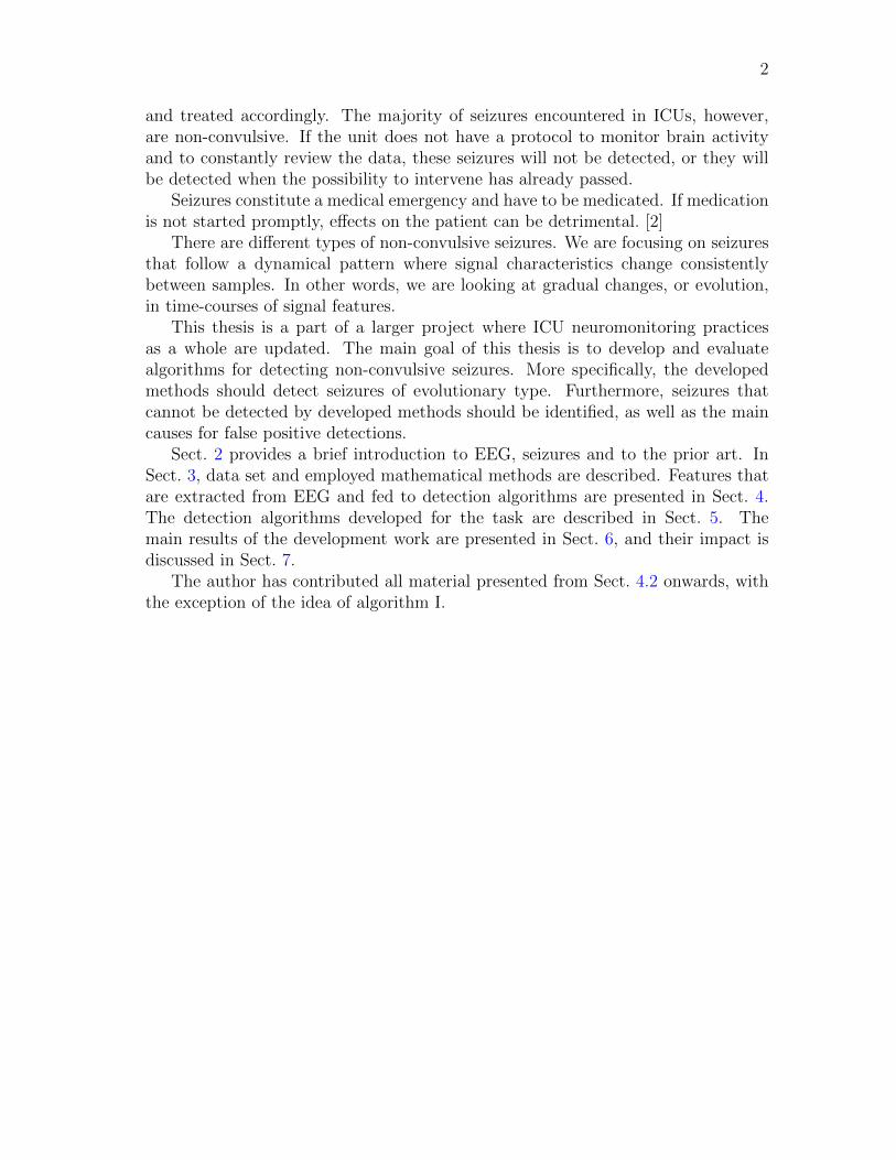
This thesis is a part of a larger project where ICU neuromonitoring practicesas a whole are updated. The main goal of this thesis is to develop and evaluatealgorithms for detecting non-convulsive seizures. More specifically, the developedmethods should detect seizures of evolutionary type. Furthermore, seizures thatcannot be detected by developed methods should be identified, as well as the maincauses for false positive detections.

Sect. 2 provides a brief introduction to EEG, seizures and to the prior art. InSect. 3, data set and employed mathematical methods are described. Features thatare extracted from EEG and fed to detection algorithms are presented in Sect. 4.The detection algorithms developed for the task are described in Sect. 5. Themain results of the development work are presented in Sect. 6, and their impact isdiscussed in Sect. 7.

The author has contributed all material presented from Sect. 4.2 onwards, withthe exception of the idea of algorithm I.

3

2 Background

This thesis is a part of a larger effort to renew brain state monitoring practicesin ICUs. A novel electrode cap and an artefact rejection algorithm were beingdeveloped in parallel with this thesis. The goal of the project as a whole is to providethe ICU staff an easy-to-use means for monitoring their patients’ neurological states.Furthermore, the staff should be able to easily interpret the information providedby the algorithms and gain objective evidence to support decision making.

Using the full conventional EEG measurement set-up is time-consuming [3]. Thenovel electrode cap is designed to be as easy as possible to put on the patient and toalign with anatomical landmarks. It can maintain a good electrical contact through-out prolonged recordings. To facilitate the set-up process and data processing, weare using only a subset of the full electrode montage.

Artefact rejection is a critical part of any biomedical signal processing applica-tion. We want to ensure that only high-quality data are passed on after this step.In the ICU, several abnormal EEG patterns are present because the patients are ina critical condition and the environment is anything but calm and controlled. Thismakes it difficult to design a reliable artefact rejection algorithm. We use additionalinformation from accelerometers integrated to the electrode cap to detect motionartefacts accurately [4].

At the heart of the concept is the signal processing algorithm. The algorithmshould provide an accurate picture of the patient’s state and address the prob-lem of non-convulsive seizures that are nowadays mostly undetected and, therefore,untreated. This thesis focuses on the development of the EEG signal processingalgorithm. The rest of this section is devoted to familiarizing the reader with theenvironment and the techniques used.

2.1 Basics of EEG

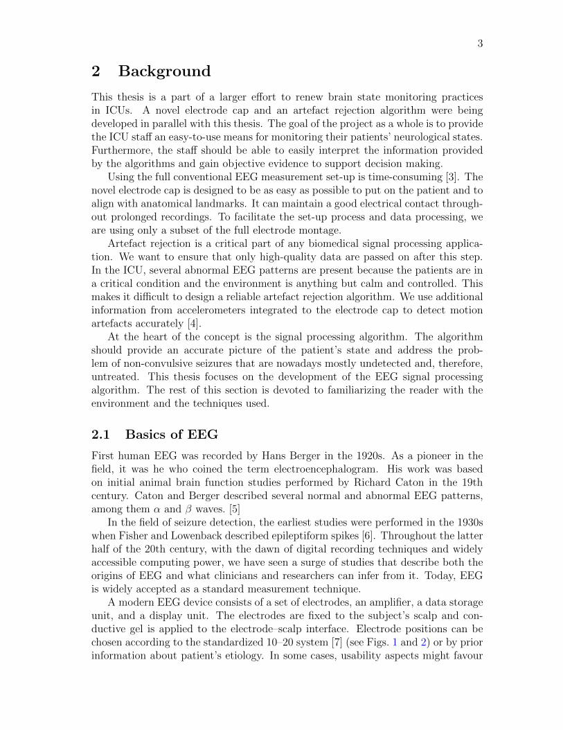
First human EEG was recorded by Hans Berger in the 1920s. As a pioneer in thefield, it was he who coined the term electroencephalogram. His work was basedon initial animal brain function studies performed by Richard Caton in the 19thcentury. Caton and Berger described several normal and abnormal EEG patterns,among them α and β waves. [5]

In the field of seizure detection, the earliest studies were performed in the 1930swhen Fisher and Lowenback described epileptiform spikes [6]. Throughout the latterhalf of the 20th century, with the dawn of digital recording techniques and widelyaccessible computing power, we have seen a surge of studies that describe both theorigins of EEG and what clinicians and researchers can infer from it. Today, EEGis widely accepted as a standard measurement technique.

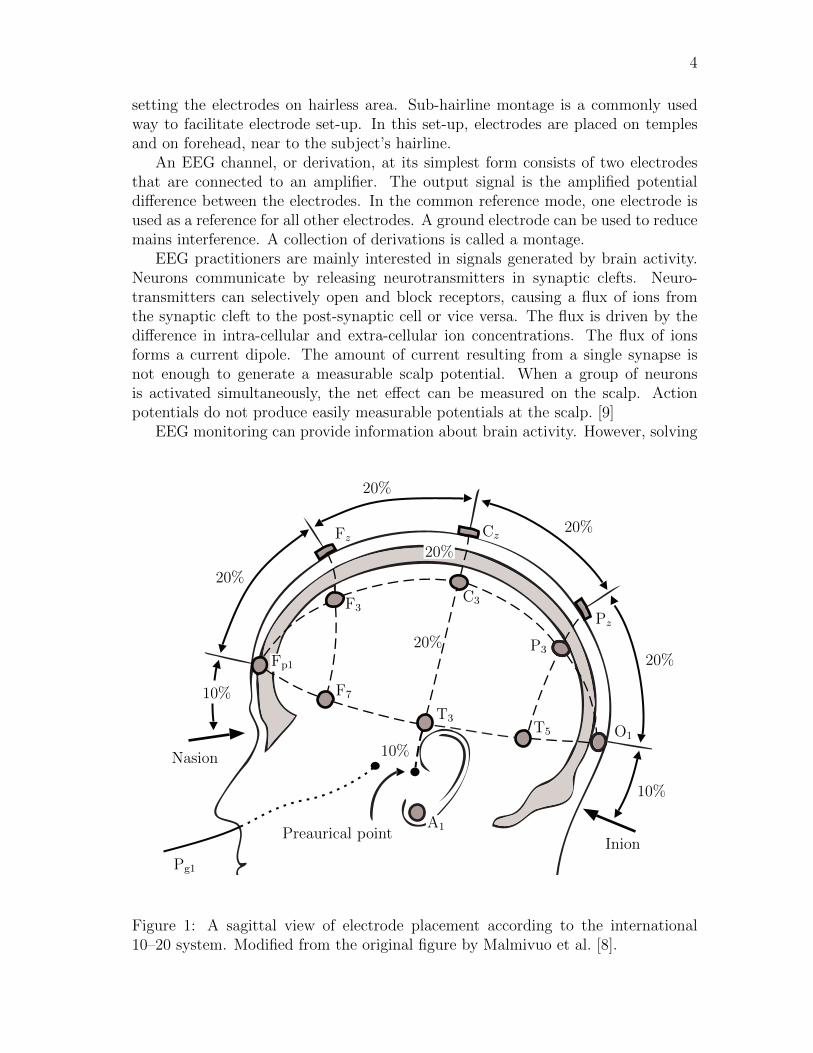
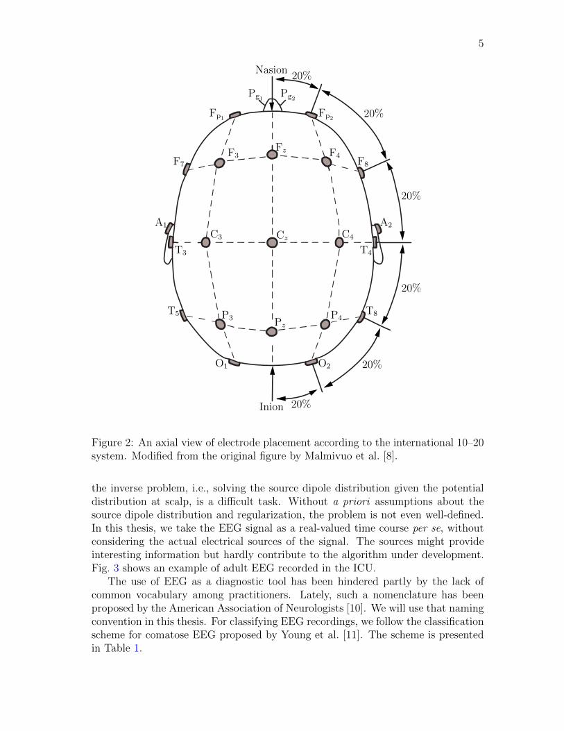
A modern EEG device consists of a set of electrodes, an amplifier, a data storageunit, and a display unit. The electrodes are fixed to the subject’s scalp and con-ductive gel is applied to the electrode–scalp interface. Electrode positions can bechosen according to the standardized 10–20 system [7] (see Figs. 1 and 2) or by priorinformation about patient’s etiology. In some cases, usability aspects might favour

4

setting the electrodes on hairless area. Sub-hairline montage is a commonly usedway to facilitate electrode set-up. In this set-up, electrodes are placed on templesand on forehead, near to the subject’s hairline.

An EEG channel, or derivation, at its simplest form consists of two electrodesthat are connected to an amplifier. The output signal is the amplified potentialdifference between the electrodes. In the common reference mode, one electrode isused as a reference for all other electrodes. A ground electrode can be used to reducemains interference. A collection of derivations is called a montage.

EEG practitioners are mainly interested in signals generated by brain activity.Neurons communicate by releasing neurotransmitters in synaptic clefts. Neuro-transmitters can selectively open and block receptors, causing a flux of ions fromthe synaptic cleft to the post-synaptic cell or vice versa. The flux is driven by thedifference in intra-cellular and extra-cellular ion concentrations. The flux of ionsforms a current dipole. The amount of current resulting from a single synapse isnot enough to generate a measurable scalp potential. When a group of neuronsis activated simultaneously, the net effect can be measured on the scalp. Actionpotentials do not produce easily measurable potentials at the scalp. [9]

EEG monitoring can provide information about brain activity. However, solving

Nasion

Preaurical pointInion

10%

20%

20%

20%

20%

10%

10%

20%

20%

Pg1

A1

Fp1

F7

T3

T5 O1

F3C3

P3

Fz Cz

Pz

Figure 1: A sagittal view of electrode placement according to the international10–20 system. Modified from the original figure by Malmivuo et al. [8].

5

Nasion

Inion

20%

20%

20%

20%

20%

20%

Pg1Pg2

Fp1Fp2

F7

F3

Fz F4

F8

A1

T3

C3 Cz C4

T4

A2

T5 P3 PzP4

T8

O1 O2

Figure 2: An axial view of electrode placement according to the international 10–20system. Modified from the original figure by Malmivuo et al. [8].

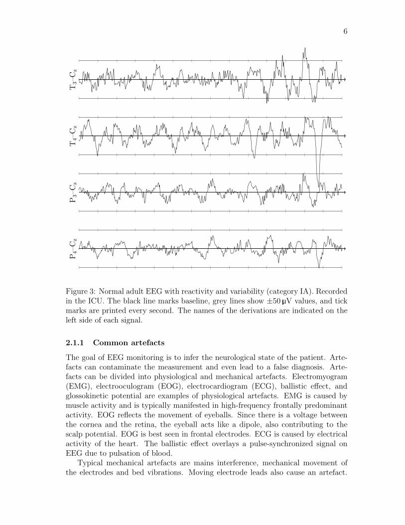
the inverse problem, i.e., solving the source dipole distribution given the potentialdistribution at scalp, is a difficult task. Without a priori assumptions about thesource dipole distribution and regularization, the problem is not even well-defined.In this thesis, we take the EEG signal as a real-valued time course per se, withoutconsidering the actual electrical sources of the signal. The sources might provideinteresting information but hardly contribute to the algorithm under development.Fig. 3 shows an example of adult EEG recorded in the ICU.

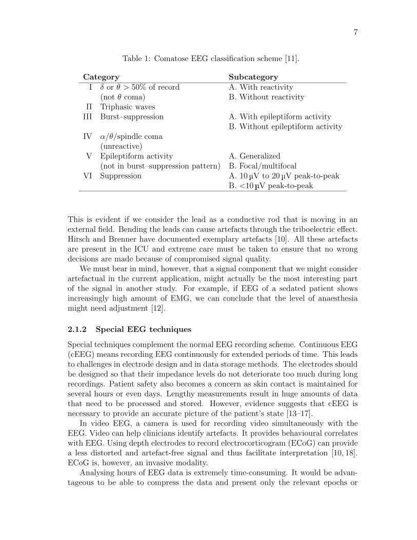
The use of EEG as a diagnostic tool has been hindered partly by the lack ofcommon vocabulary among practitioners. Lately, such a nomenclature has beenproposed by the American Association of Neurologists [10]. We will use that namingconvention in this thesis. For classifying EEG recordings, we follow the classificationscheme for comatose EEG proposed by Young et al. [11]. The scheme is presentedin Table 1.

6

T3–C

zT

4–C

zP3–C

zP4–C

z

Figure 3: Normal adult EEG with reactivity and variability (category IA). Recordedin the ICU. The black line marks baseline, grey lines show ±50 V values, and tickmarks are printed every second. The names of the derivations are indicated on theleft side of each signal.

2.1.1 Common artefacts

The goal of EEG monitoring is to infer the neurological state of the patient. Arte-facts can contaminate the measurement and even lead to a false diagnosis. Arte-facts can be divided into physiological and mechanical artefacts. Electromyogram(EMG), electrooculogram (EOG), electrocardiogram (ECG), ballistic effect, andglossokinetic potential are examples of physiological artefacts. EMG is caused bymuscle activity and is typically manifested in high-frequency frontally predominantactivity. EOG reflects the movement of eyeballs. Since there is a voltage betweenthe cornea and the retina, the eyeball acts like a dipole, also contributing to thescalp potential. EOG is best seen in frontal electrodes. ECG is caused by electricalactivity of the heart. The ballistic effect overlays a pulse-synchronized signal onEEG due to pulsation of blood.

Typical mechanical artefacts are mains interference, mechanical movement ofthe electrodes and bed vibrations. Moving electrode leads also cause an artefact.

7

Table 1: Comatose EEG classification scheme [11].

Category Subcategory

I δ or θ > 50% of record A. With reactivity(not θ coma) B. Without reactivity

II Triphasic wavesIII Burst–suppression A. With epileptiform activity

B. Without epileptiform activityIV α/θ/spindle coma

(unreactive)V Epileptiform activity A. Generalized

(not in burst–suppression pattern) B. Focal/multifocalVI Suppression A. 10 V to 20 V peak-to-peak

B. <10 V peak-to-peak

This is evident if we consider the lead as a conductive rod that is moving in anexternal field. Bending the leads can cause artefacts through the triboelectric effect.Hirsch and Brenner have documented exemplary artefacts [10]. All these artefactsare present in the ICU and extreme care must be taken to ensure that no wrongdecisions are made because of compromised signal quality.

We must bear in mind, however, that a signal component that we might considerartefactual in the current application, might actually be the most interesting partof the signal in another study. For example, if EEG of a sedated patient showsincreasingly high amount of EMG, we can conclude that the level of anaesthesiamight need adjustment [12].

2.1.2 Special EEG techniques

Special techniques complement the normal EEG recording scheme. Continuous EEG(cEEG) means recording EEG continuously for extended periods of time. This leadsto challenges in electrode design and in data storage methods. The electrodes shouldbe designed so that their impedance levels do not deteriorate too much during longrecordings. Patient safety also becomes a concern as skin contact is maintained forseveral hours or even days. Lengthy measurements result in huge amounts of datathat need to be processed and stored. However, evidence suggests that cEEG isnecessary to provide an accurate picture of the patient’s state [13–17].

In video EEG, a camera is used for recording video simultaneously with theEEG. Video can help clinicians identify artefacts. It provides behavioural correlateswith EEG. Using depth electrodes to record electrocorticogram (ECoG) can providea less distorted and artefact-free signal and thus facilitate interpretation [10, 18].ECoG is, however, an invasive modality.

Analysing hours of EEG data is extremely time-consuming. It would be advan-tageous to be able to compress the data and present only the relevant epochs or

8

trends to clinicians. Agarwal and Gotman have presented one example for summa-rizing EEG data [19]. Even though such semi-automatic post-processing methodshave been designed, the fact remains that raw EEG signal must be available forlater review.

2.2 Seizures

Epilepsy is a term used for a group of neurological disorders. Individuals witha diagnosis of epilepsy have recurrent, unprovoked seizures [1]. A seizure is anabnormal electrical discharge in the brain [20]. Some people have genetic featuresthat elevate the risk of developing epilepsy. Epilepsy can also emerge due to astructural abnormality. Idiopathic epilepsy means that the cause of the disorderis unknown. Types of seizures, their intensity, frequency, and duration vary a lotbetween patients, but it is common that the same pattern is repeated on eachoccasion on a given patient. About 0.6% of the general population suffers fromepilepsy. The prevalence varies, however, between age groups. [21, 22]

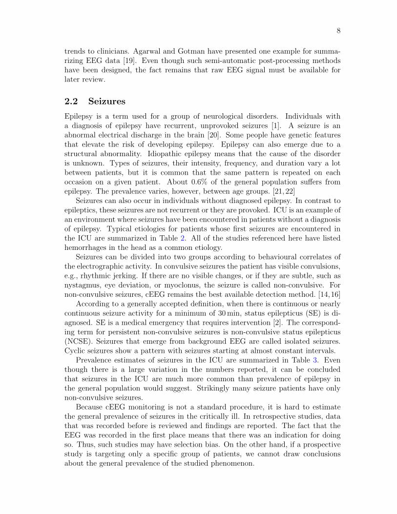
Seizures can also occur in individuals without diagnosed epilepsy. In contrast toepileptics, these seizures are not recurrent or they are provoked. ICU is an example ofan environment where seizures have been encountered in patients without a diagnosisof epilepsy. Typical etiologies for patients whose first seizures are encountered inthe ICU are summarized in Table 2. All of the studies referenced here have listedhemorrhages in the head as a common etiology.

Seizures can be divided into two groups according to behavioural correlates ofthe electrographic activity. In convulsive seizures the patient has visible convulsions,e.g., rhythmic jerking. If there are no visible changes, or if they are subtle, such asnystagmus, eye deviation, or myoclonus, the seizure is called non-convulsive. Fornon-convulsive seizures, cEEG remains the best available detection method. [14,16]

According to a generally accepted definition, when there is continuous or nearlycontinuous seizure activity for a minimum of 30min, status epilepticus (SE) is di-agnosed. SE is a medical emergency that requires intervention [2]. The correspond-ing term for persistent non-convulsive seizures is non-convulsive status epilepticus(NCSE). Seizures that emerge from background EEG are called isolated seizures.Cyclic seizures show a pattern with seizures starting at almost constant intervals.

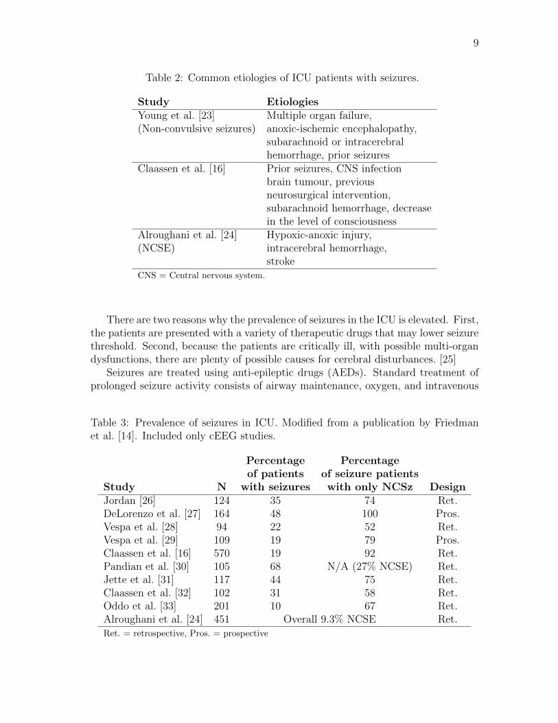
Prevalence estimates of seizures in the ICU are summarized in Table 3. Eventhough there is a large variation in the numbers reported, it can be concludedthat seizures in the ICU are much more common than prevalence of epilepsy inthe general population would suggest. Strikingly many seizure patients have onlynon-convulsive seizures.

Because cEEG monitoring is not a standard procedure, it is hard to estimatethe general prevalence of seizures in the critically ill. In retrospective studies, datathat was recorded before is reviewed and findings are reported. The fact that theEEG was recorded in the first place means that there was an indication for doingso. Thus, such studies may have selection bias. On the other hand, if a prospectivestudy is targeting only a specific group of patients, we cannot draw conclusionsabout the general prevalence of the studied phenomenon.

9

Table 2: Common etiologies of ICU patients with seizures.

Study Etiologies

Young et al. [23] Multiple organ failure,(Non-convulsive seizures) anoxic-ischemic encephalopathy,

subarachnoid or intracerebralhemorrhage, prior seizures

Claassen et al. [16] Prior seizures, CNS infectionbrain tumour, previousneurosurgical intervention,subarachnoid hemorrhage, decreasein the level of consciousness

Alroughani et al. [24] Hypoxic-anoxic injury,(NCSE) intracerebral hemorrhage,

strokeCNS = Central nervous system.

There are two reasons why the prevalence of seizures in the ICU is elevated. First,the patients are presented with a variety of therapeutic drugs that may lower seizurethreshold. Second, because the patients are critically ill, with possible multi-organdysfunctions, there are plenty of possible causes for cerebral disturbances. [25]

Seizures are treated using anti-epileptic drugs (AEDs). Standard treatment ofprolonged seizure activity consists of airway maintenance, oxygen, and intravenous

Table 3: Prevalence of seizures in ICU. Modified from a publication by Friedmanet al. [14]. Included only cEEG studies.

Percentage Percentage

of patients of seizure patients

Study N with seizures with only NCSz Design

Jordan [26] 124 35 74 Ret.DeLorenzo et al. [27] 164 48 100 Pros.Vespa et al. [28] 94 22 52 Ret.Vespa et al. [29] 109 19 79 Pros.Claassen et al. [16] 570 19 92 Ret.Pandian et al. [30] 105 68 N/A (27% NCSE) Ret.Jette et al. [31] 117 44 75 Ret.Claassen et al. [32] 102 31 58 Ret.Oddo et al. [33] 201 10 67 Ret.Alroughani et al. [24] 451 Overall 9.3% NCSE Ret.Ret. = retrospective, Pros. = prospective

10

diazepam. During medication, the cause of seizures should be investigated. If thecondition worsens, intravenous anaesthesia, intubation, and ventilation are required.Thiopentone or propofol can be titrated until a burst–suppression pattern is seen inEEG. [2]

Accumulating evidence suggests that also non-convulsive seizures and seizureactivity that does not qualify as SE should be treated. A widely supported viewis to consider seizure activity longer than 5–10 min as a condition that requiresintervention [15]. Periodic epileptiform discharges (PLEDs) might not count as aseizure, but initiating prophylaxis has been suggested as a reasonable action if suchpatterns are found [34].

For non-convulsive seizures, seizure duration and delay to diagnosis have beenfound to be associated with increased mortality. However, it should be noted thatthis patient population consists of critically ill. It might be practically impossibleto tell whether the mortalities are caused by the original underlying etiologies or bythe neurological dysfunctions resulting from them. [14, 23]

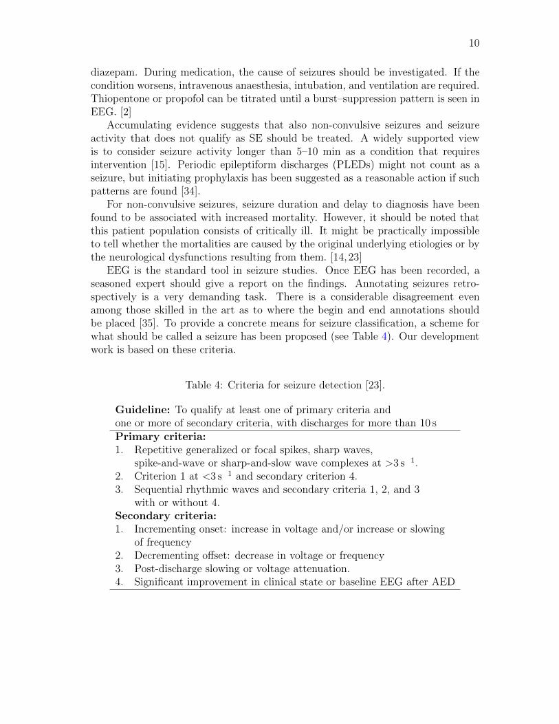
EEG is the standard tool in seizure studies. Once EEG has been recorded, aseasoned expert should give a report on the findings. Annotating seizures retro-spectively is a very demanding task. There is a considerable disagreement evenamong those skilled in the art as to where the begin and end annotations shouldbe placed [35]. To provide a concrete means for seizure classification, a scheme forwhat should be called a seizure has been proposed (see Table 4). Our developmentwork is based on these criteria.

Table 4: Criteria for seizure detection [23].

Guideline: To qualify at least one of primary criteria andone or more of secondary criteria, with discharges for more than 10 sPrimary criteria:

1. Repetitive generalized or focal spikes, sharp waves,spike-and-wave or sharp-and-slow wave complexes at >3 s 1.

2. Criterion 1 at <3 s 1 and secondary criterion 4.3. Sequential rhythmic waves and secondary criteria 1, 2, and 3

with or without 4.Secondary criteria:

1. Incrementing onset: increase in voltage and/or increase or slowingof frequency

2. Decrementing offset: decrease in voltage or frequency3. Post-discharge slowing or voltage attenuation.4. Significant improvement in clinical state or baseline EEG after AED

11

2.2.1 Epileptiform EEG

The adjective epileptiform means something that is related to epilepsy [36]. Epilep-tiform EEG thus refers to EEG patterns that are often found in epileptics. Epilep-tiform patterns are abnormal, but as such they do not constitute a seizure. Even apatient without seizures can have some epileptiform patterns present in the EEG.EEG during seizure is called ictal and between seizures inter-ictal.

This subsection summarizes some common EEG findings in the critically ill.More examples on how to interpret EEG findings in the critically ill are reported byHirsch and Brenner [10] and by Chong and Hirsch [34].

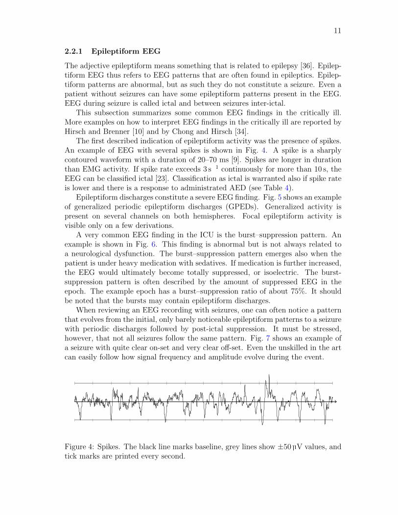
The first described indication of epileptiform activity was the presence of spikes.An example of EEG with several spikes is shown in Fig. 4. A spike is a sharplycontoured waveform with a duration of 20–70 ms [9]. Spikes are longer in durationthan EMG activity. If spike rate exceeds 3 s 1 continuously for more than 10 s, theEEG can be classified ictal [23]. Classification as ictal is warranted also if spike rateis lower and there is a response to administrated AED (see Table 4).

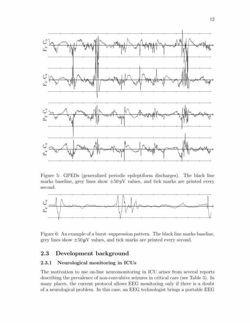
Epileptiform discharges constitute a severe EEG finding. Fig. 5 shows an exampleof generalized periodic epileptiform discharges (GPEDs). Generalized activity ispresent on several channels on both hemispheres. Focal epileptiform activity isvisible only on a few derivations.

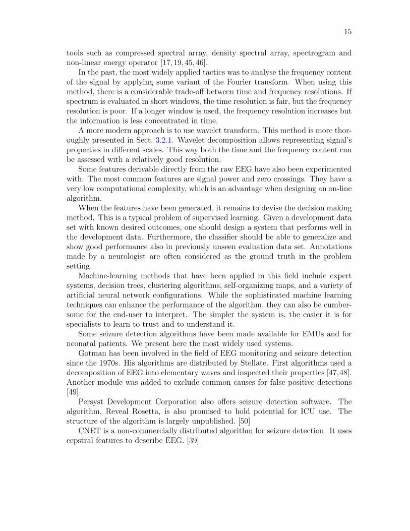
A very common EEG finding in the ICU is the burst–suppression pattern. Anexample is shown in Fig. 6. This finding is abnormal but is not always related toa neurological dysfunction. The burst–suppression pattern emerges also when thepatient is under heavy medication with sedatives. If medication is further increased,the EEG would ultimately become totally suppressed, or isoelectric. The burst-suppression pattern is often described by the amount of suppressed EEG in theepoch. The example epoch has a burst–suppression ratio of about 75%. It shouldbe noted that the bursts may contain epileptiform discharges.

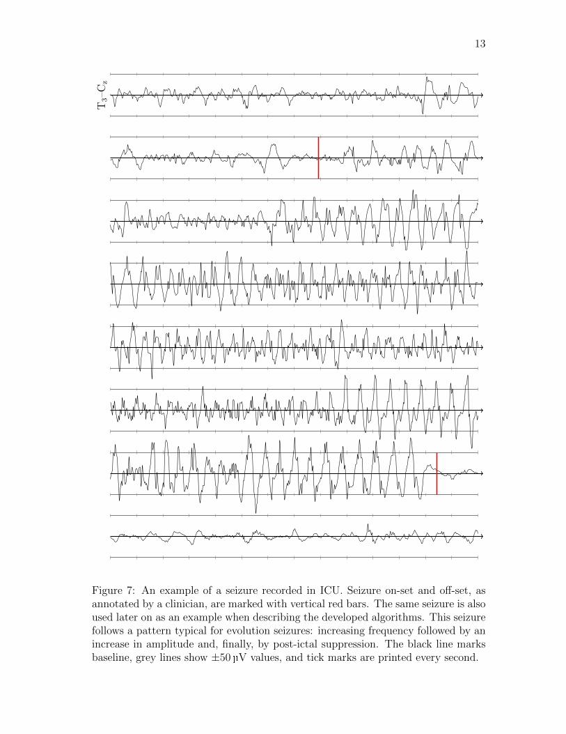
When reviewing an EEG recording with seizures, one can often notice a patternthat evolves from the initial, only barely noticeable epileptiform patterns to a seizurewith periodic discharges followed by post-ictal suppression. It must be stressed,however, that not all seizures follow the same pattern. Fig. 7 shows an example ofa seizure with quite clear on-set and very clear off-set. Even the unskilled in the artcan easily follow how signal frequency and amplitude evolve during the event.

Figure 4: Spikes. The black line marks baseline, grey lines show ±50 V values, andtick marks are printed every second.

12

F3–C

zF4–C

zP3–C

zP4–C

z

Figure 5: GPEDs (generalized periodic epileptiform discharges). The black linemarks baseline, grey lines show ±50 V values, and tick marks are printed everysecond.

P4–C

z

Figure 6: An example of a burst–suppression pattern. The black line marks baseline,grey lines show ±50 V values, and tick marks are printed every second.

2.3 Development background

2.3.1 Neurological monitoring in ICUs

The motivation to use on-line neuromonitoring in ICU arises from several reportsdescribing the prevalence of non-convulsive seizures in critical care (see Table 3). Inmany places, the current protocol allows EEG monitoring only if there is a doubtof a neurological problem. In this case, an EEG technologist brings a portable EEG

13

T3–C

z

Figure 7: An example of a seizure recorded in ICU. Seizure on-set and off-set, asannotated by a clinician, are marked with vertical red bars. The same seizure is alsoused later on as an example when describing the developed algorithms. This seizurefollows a pattern typical for evolution seizures: increasing frequency followed by anincrease in amplitude and, finally, by post-ictal suppression. The black line marksbaseline, grey lines show ±50 V values, and tick marks are printed every second.

14

system to the ICU, connects the electrodes and records for approximately 30min.The data are later reviewed by a neurologist who decides which actions should betaken. There are typically 1–2 assessments per day in a non-neurological ICU [14].

This scheme is inefficient for two reasons. First, there is no guarantee that aseizure appears during those 30min. In a retrospective study, it was found thatonly 56% of seizure patients had their first seizure during the first hour of the cEEGrecording. After 48 h, 93% of the patients had encountered their first seizure [16].Second, in the current scheme, there is a considerable delay between the recordingand the possible intervention.

2.3.2 Prior art

Several algorithms have already been designed for seizure detection in epilepsy mon-itoring units (EMUs) and for neonatal patients. ICU, however, has so far been out oftheir scope. Gotman, a recognized researcher in the field, has reviewed the generalprinciples of seizure detection [37,38].

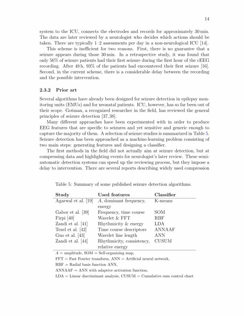
Many different approaches have been experimented with in order to produceEEG features that are specific to seizures and yet sensitive and generic enough tocapture the majority of them. A selection of seizure studies is summarized in Table 5.Seizure detection has been approached as a machine-learning problem consisting oftwo main steps: generating features and designing a classifier.

The first methods in the field did not actually aim at seizure detection, but atcompressing data and highlighting events for neurologist’s later review. These semi-automatic detection systems can speed up the reviewing process, but they impose adelay to intervention. There are several reports describing widely used compression

Table 5: Summary of some published seizure detection algorithms.

Study Used features Classifier

Agarwal et al. [19] A, dominant frequency, K-meansenergy

Gabor et al. [39] Frequency, time course SOMFirpi [40] Wavelet & FFT RBFZandi et al. [41] Rhythmicity & energy LDATezel et al. [42] Time course descriptors ANNAAFGuo et al. [43] Wavelet line length ANNZandi et al. [44] Rhythmicity, consistency, CUSUM

relative energyA = amplitude, SOM = Self-organizing map,

FFT = Fast Fourier transform, ANN = Artificial neural network,

RBF = Radial basis function ANN,

ANNAAF = ANN with adaptive activation function,

LDA = Linear discriminant analysis, CUSUM = Cumulative sum control chart

15

tools such as compressed spectral array, density spectral array, spectrogram andnon-linear energy operator [17, 19, 45, 46].

In the past, the most widely applied tactics was to analyse the frequency contentof the signal by applying some variant of the Fourier transform. When using thismethod, there is a considerable trade-off between time and frequency resolutions. Ifspectrum is evaluated in short windows, the time resolution is fair, but the frequencyresolution is poor. If a longer window is used, the frequency resolution increases butthe information is less concentrated in time.

A more modern approach is to use wavelet transform. This method is more thor-oughly presented in Sect. 3.2.1. Wavelet decomposition allows representing signal’sproperties in different scales. This way both the time and the frequency content canbe assessed with a relatively good resolution.

Some features derivable directly from the raw EEG have also been experimentedwith. The most common features are signal power and zero crossings. They have avery low computational complexity, which is an advantage when designing an on-linealgorithm.

When the features have been generated, it remains to devise the decision makingmethod. This is a typical problem of supervised learning. Given a development dataset with known desired outcomes, one should design a system that performs well inthe development data. Furthermore, the classifier should be able to generalize andshow good performance also in previously unseen evaluation data set. Annotationsmade by a neurologist are often considered as the ground truth in the problemsetting.

Machine-learning methods that have been applied in this field include expertsystems, decision trees, clustering algorithms, self-organizing maps, and a variety ofartificial neural network configurations. While the sophisticated machine learningtechniques can enhance the performance of the algorithm, they can also be cumber-some for the end-user to interpret. The simpler the system is, the easier it is forspecialists to learn to trust and to understand it.

Some seizure detection algorithms have been made available for EMUs and forneonatal patients. We present here the most widely used systems.

Gotman has been involved in the field of EEG monitoring and seizure detectionsince the 1970s. His algorithms are distributed by Stellate. First algorithms used adecomposition of EEG into elementary waves and inspected their properties [47,48].Another module was added to exclude common causes for false positive detections[49].

Persyst Development Corporation also offers seizure detection software. Thealgorithm, Reveal Rosetta, is also promised to hold potential for ICU use. Thestructure of the algorithm is largely unpublished. [50]

CNET is a non-commercially distributed algorithm for seizure detection. It usescepstral features to describe EEG. [39]

16

2.3.3 Design drivers for the new algorithm

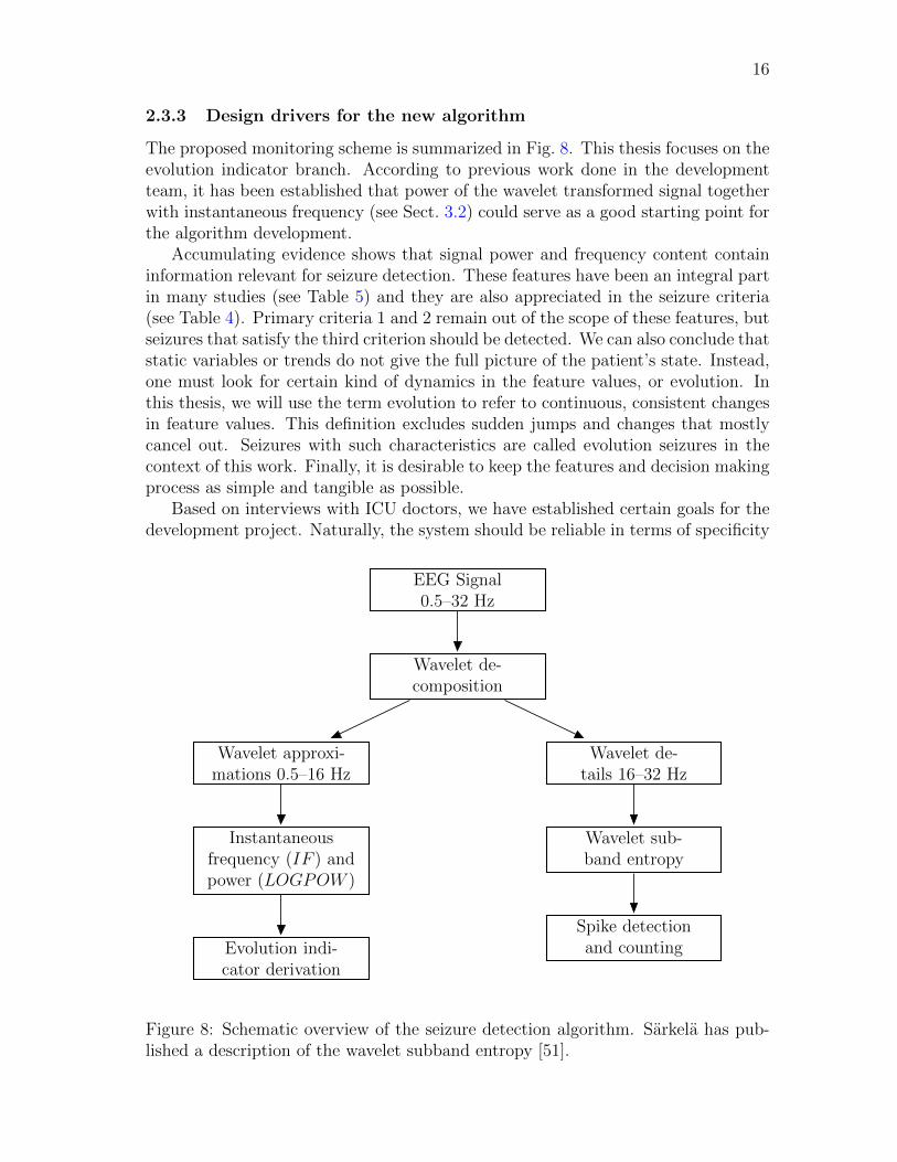
The proposed monitoring scheme is summarized in Fig. 8. This thesis focuses on theevolution indicator branch. According to previous work done in the developmentteam, it has been established that power of the wavelet transformed signal togetherwith instantaneous frequency (see Sect. 3.2) could serve as a good starting point forthe algorithm development.

Accumulating evidence shows that signal power and frequency content containinformation relevant for seizure detection. These features have been an integral partin many studies (see Table 5) and they are also appreciated in the seizure criteria(see Table 4). Primary criteria 1 and 2 remain out of the scope of these features, butseizures that satisfy the third criterion should be detected. We can also conclude thatstatic variables or trends do not give the full picture of the patient’s state. Instead,one must look for certain kind of dynamics in the feature values, or evolution. Inthis thesis, we will use the term evolution to refer to continuous, consistent changesin feature values. This definition excludes sudden jumps and changes that mostlycancel out. Seizures with such characteristics are called evolution seizures in thecontext of this work. Finally, it is desirable to keep the features and decision makingprocess as simple and tangible as possible.

Based on interviews with ICU doctors, we have established certain goals for thedevelopment project. Naturally, the system should be reliable in terms of specificity

EEG Signal0.5–32 Hz

Wavelet de-composition

Wavelet de-tails 16–32 Hz

Wavelet approxi-mations 0.5–16 Hz

Wavelet sub-band entropy

Spike detectionand counting

Instantaneousfrequency (IF ) andpower (LOGPOW )

Evolution indi-cator derivation

Figure 8: Schematic overview of the seizure detection algorithm. Sarkela has pub-lished a description of the wavelet subband entropy [51].

17

and sensitivity. It must be able to detect both isolated seizures and prolonged ictalactivity. Ability to compress data and to present long-term trends that monitor howthe patient’s state has progressed would be a desirable feature. Finally, the systemshould be user-friendly both in terms of visualization and in using the electrode cap.

The project aims at developing monitoring software that presents relevant infor-mation at the bedside and at the event of seizure activity alerts both the bedsidestaff and a neurologist. A summary containing the raw EEG could be sent to theneurologist who has remote access to the information system. After administeringAED, the effect could be followed by both the neurologist and the bedside staff onreal time. The bedside staff cannot be constantly paying attention to the moni-tor, and neurologists do not want any unnecessary disturbance caused by irrelevantevents. For these reasons, it is important to minimize false positive alerts.

By interviewing experts in the field, we have established the following goals forthe seizure detection algorithm:

• Every patient with seizures should be detected

• On each seizure patient, we should reach 80–90% sensitivity

• An acceptable rate of false positive detections is about 1 in 8 h

These are the ultimate goals of the project. At this stage, however, we can relaxthe specifications since we are designing only one part of the final method. Spikedetection, for example, is an integral part of the final method but is not included inthe analyses conducted in this thesis.

18

3 Materials and methods

3.1 Data set

The data for this study have been collected at London Health Sciences Centre,Ontario, Canada. The patients included in the study were receiving critical care.

Data were collected using two different devices. A sub-hairline EEG was recordedby a device manufactured by Datex-Ohmeda. Standard scalp EEG was recordedby a device manufactured by XL-Tek. Data from both recordings were analysedretrospectively by an expert neurologist, Dr. G. Bryan Young. Two devices wereused to study how sensitive and specific the limited-coverage sub-hairline montageis compared to the standard 10–20 system.

Because of recent reports implying that sub-hairline EEG has low sensitivityfor detecting seizures [14, 52, 53], we will use normal scalp EEG recordings as thedevelopment data. Unfortunately, in some recordings, periods of data had beenremoved before the data were delivered. For our use, we extracted from the originaldata files derivations F3–Cz, F4–Cz, T3–Cz, T4–Cz, P3–Cz, and P4–Cz.

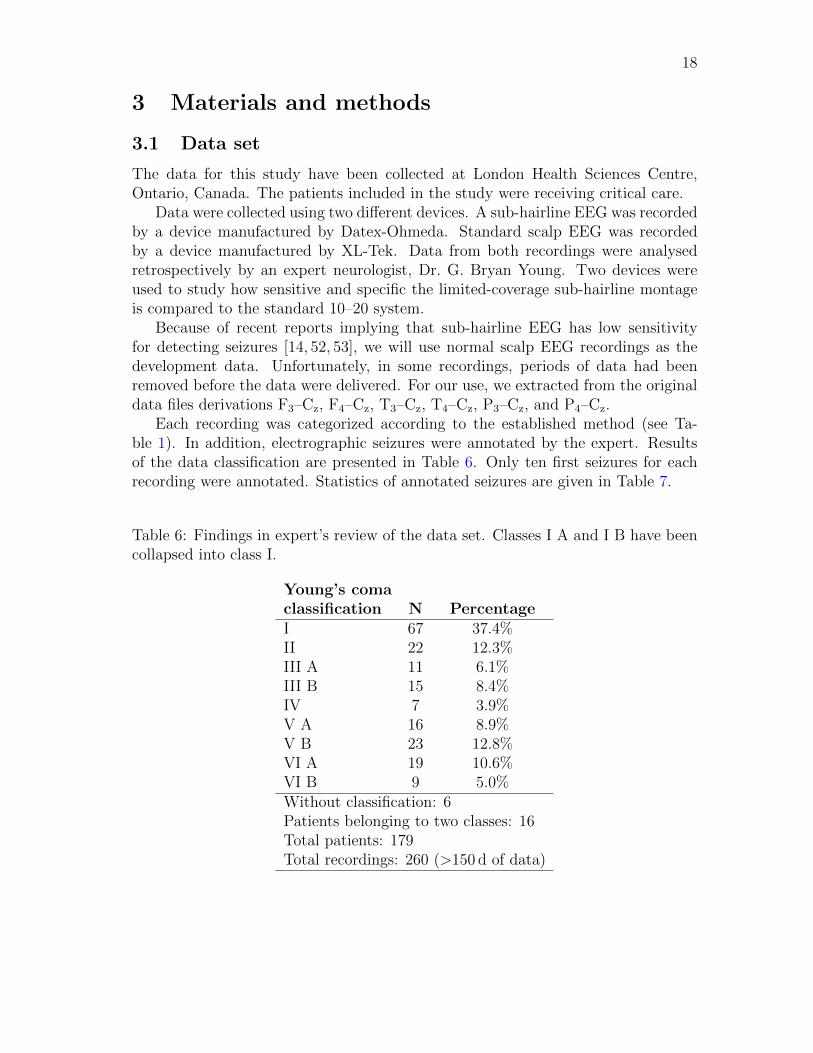
Each recording was categorized according to the established method (see Ta-ble 1). In addition, electrographic seizures were annotated by the expert. Resultsof the data classification are presented in Table 6. Only ten first seizures for eachrecording were annotated. Statistics of annotated seizures are given in Table 7.

Table 6: Findings in expert’s review of the data set. Classes I A and I B have beencollapsed into class I.

Young’s coma

classification N Percentage

I 67 37.4%II 22 12.3%III A 11 6.1%III B 15 8.4%IV 7 3.9%V A 16 8.9%V B 23 12.8%VI A 19 10.6%VI B 9 5.0%Without classification: 6Patients belonging to two classes: 16Total patients: 179Total recordings: 260 (>150 d of data)

19

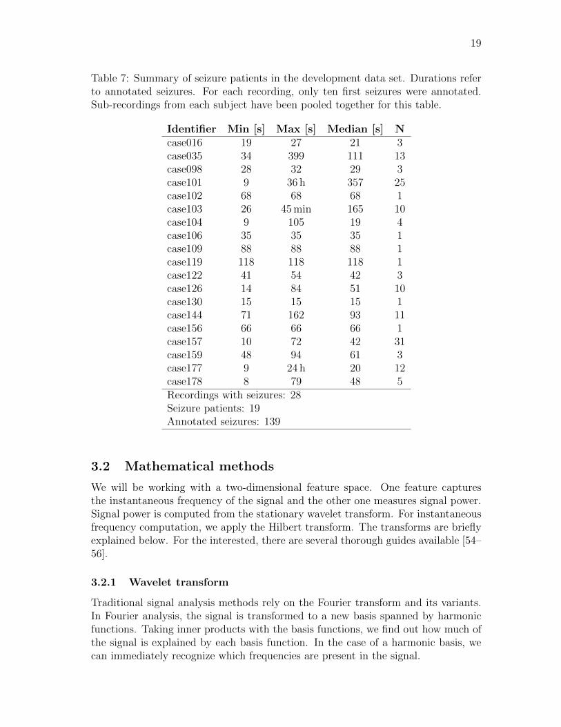
Table 7: Summary of seizure patients in the development data set. Durations referto annotated seizures. For each recording, only ten first seizures were annotated.Sub-recordings from each subject have been pooled together for this table.

Identifier Min [s] Max [s] Median [s] N

case016 19 27 21 3case035 34 399 111 13case098 28 32 29 3case101 9 36 h 357 25case102 68 68 68 1case103 26 45min 165 10case104 9 105 19 4case106 35 35 35 1case109 88 88 88 1case119 118 118 118 1case122 41 54 42 3case126 14 84 51 10case130 15 15 15 1case144 71 162 93 11case156 66 66 66 1case157 10 72 42 31case159 48 94 61 3case177 9 24 h 20 12case178 8 79 48 5Recordings with seizures: 28Seizure patients: 19Annotated seizures: 139

3.2 Mathematical methods

We will be working with a two-dimensional feature space. One feature capturesthe instantaneous frequency of the signal and the other one measures signal power.Signal power is computed from the stationary wavelet transform. For instantaneousfrequency computation, we apply the Hilbert transform. The transforms are brieflyexplained below. For the interested, there are several thorough guides available [54–56].

3.2.1 Wavelet transform

Traditional signal analysis methods rely on the Fourier transform and its variants.In Fourier analysis, the signal is transformed to a new basis spanned by harmonicfunctions. Taking inner products with the basis functions, we find out how much ofthe signal is explained by each basis function. In the case of a harmonic basis, wecan immediately recognize which frequencies are present in the signal.

20

A drawback with harmonic basis functions is their lack of time resolution. Be-cause the basis functions are not localized in time, we cannot pinpoint how and whenthe frequency content changes within the computation window. Sliding windows,different windowing functions, and the short-time variant of the Fourier transformhave solved some of the issues.

Wavelet analysis approaches signal decomposition from another point of view.Instead of non-localized harmonic functions, wavelet analysis makes use of square-integrable, localized basis functions. The basis is formed by translations and dila-tions of one basis-generating function called the mother wavelet.

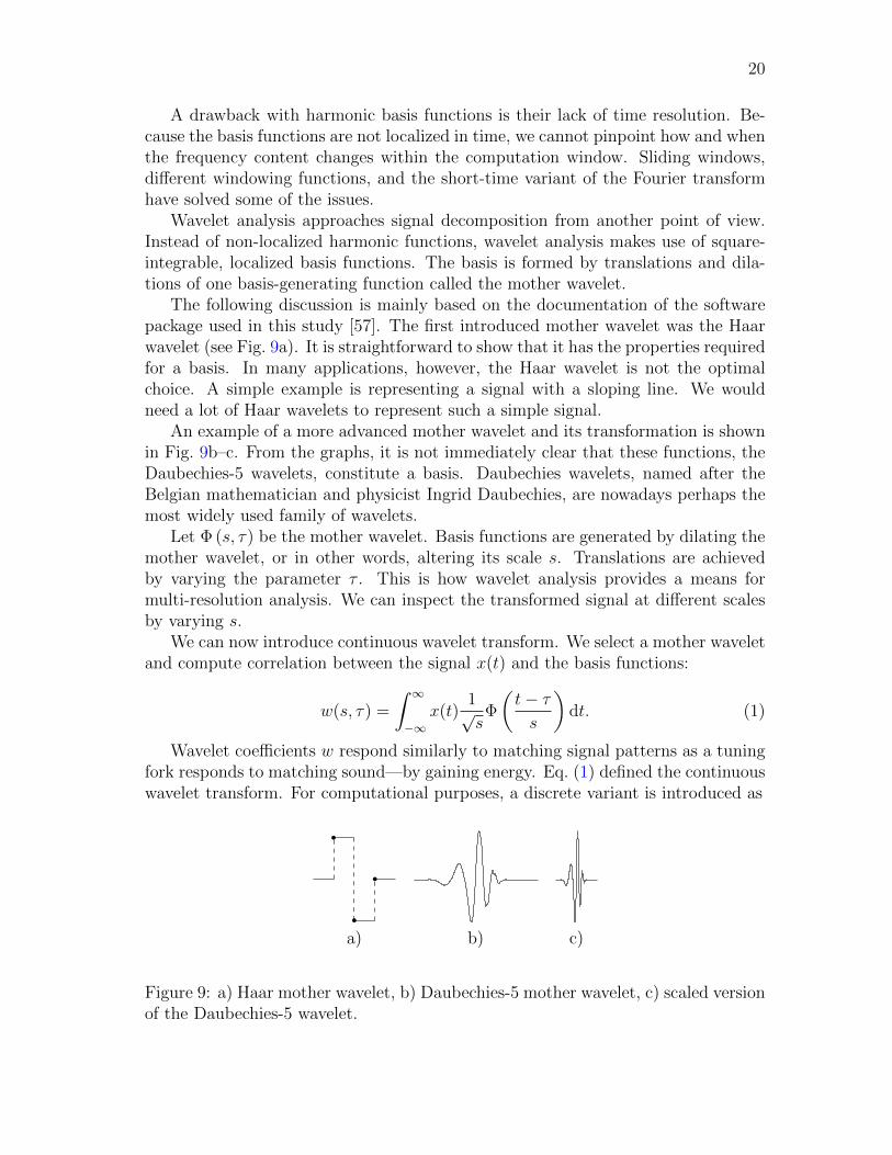
The following discussion is mainly based on the documentation of the softwarepackage used in this study [57]. The first introduced mother wavelet was the Haarwavelet (see Fig. 9a). It is straightforward to show that it has the properties requiredfor a basis. In many applications, however, the Haar wavelet is not the optimalchoice. A simple example is representing a signal with a sloping line. We wouldneed a lot of Haar wavelets to represent such a simple signal.

An example of a more advanced mother wavelet and its transformation is shownin Fig. 9b–c. From the graphs, it is not immediately clear that these functions, theDaubechies-5 wavelets, constitute a basis. Daubechies wavelets, named after theBelgian mathematician and physicist Ingrid Daubechies, are nowadays perhaps themost widely used family of wavelets.

Let Φ (s, τ) be the mother wavelet. Basis functions are generated by dilating themother wavelet, or in other words, altering its scale s. Translations are achievedby varying the parameter τ . This is how wavelet analysis provides a means formulti-resolution analysis. We can inspect the transformed signal at different scalesby varying s.

We can now introduce continuous wavelet transform. We select a mother waveletand compute correlation between the signal x(t) and the basis functions:

w(s, τ) =

� ∞

−∞x(t)

1√sΦ

�t− τ

s

�dt. (1)

Wavelet coefficients w respond similarly to matching signal patterns as a tuningfork responds to matching sound—by gaining energy. Eq. (1) defined the continuouswavelet transform. For computational purposes, a discrete variant is introduced as

a) b) c)

Figure 9: a) Haar mother wavelet, b) Daubechies-5 mother wavelet, c) scaled versionof the Daubechies-5 wavelet.

21

wj,k =

� ∞

−∞x(t)Φj,k(t)dt, (2)

where according to the widely used dyadic sampling s = 2−j, τ = k2−j, and Φj,k =sj/2Φ(2jt− k). The variables j and k are integers.

So far we have discussed wavelets using graphs of mother wavelets and correla-tions with the signal under study. It can be shown that the discrete wavelet trans-form can also be formulated as a filtering problem. This implementation, the filterbank method, is computationally very efficient. Mallat was the one to introducethis algorithm [58].

One run through the filter bank breaks the signal x[t] into two parts: approxima-tion xa[t] and details xd[t]. Approximation is the coarse scale that contains mainlythe trend of the signal. More specifically, it contains frequencies smaller than halfthe bandwidth of the signal. Details capture the fine scales, or the upper half of thebandwidth. Hence, each run divides the bandwidth of the signal in two. At stepj + 1, we have

xaj [t] = xa

j+1[t] + xd

j+1[t]. (3)

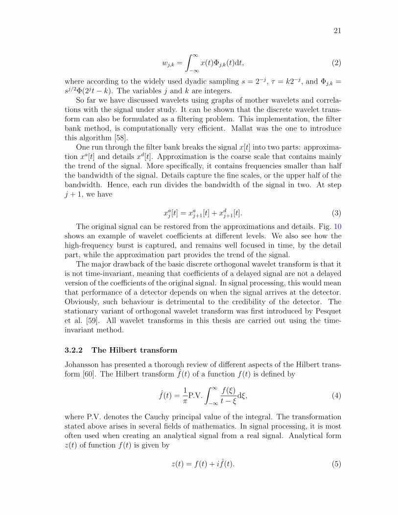
The original signal can be restored from the approximations and details. Fig. 10shows an example of wavelet coefficients at different levels. We also see how thehigh-frequency burst is captured, and remains well focused in time, by the detailpart, while the approximation part provides the trend of the signal.

The major drawback of the basic discrete orthogonal wavelet transform is that itis not time-invariant, meaning that coefficients of a delayed signal are not a delayedversion of the coefficients of the original signal. In signal processing, this would meanthat performance of a detector depends on when the signal arrives at the detector.Obviously, such behaviour is detrimental to the credibility of the detector. Thestationary variant of orthogonal wavelet transform was first introduced by Pesquetet al. [59]. All wavelet transforms in this thesis are carried out using the time-invariant method.

3.2.2 The Hilbert transform

Johansson has presented a thorough review of different aspects of the Hilbert trans-form [60]. The Hilbert transform f(t) of a function f(t) is defined by

f(t) =1

πP.V.

� ∞

−∞

f(ξ)

t− ξdξ, (4)

where P.V. denotes the Cauchy principal value of the integral. The transformationstated above arises in several fields of mathematics. In signal processing, it is mostoften used when creating an analytical signal from a real signal. Analytical formz(t) of function f(t) is given by

z(t) = f(t) + if(t). (5)

22

a)

b)

c)

Figure 10: An illustration of stationary wavelet transform with Daubechies-5 motherwavelet. a) Signal containing a high-frequency burst superposed on a stationarysignal with Gaussian noise. b) First detail level captures most of the noise and theburst. c) Second-level approximation. Units in this figure are arbitrary.

Analytical signals can be written using complex exponential function:

z(t) = A(t)eiφ(t), (6)

where

A(t) =�f(t)2 + f(t)2 (7)

and

ϕ(t) = arctan

�f(t)

f(t)

�. (8)

Knowing the phase of the signal, we can compute the instantaneous angularfrequency as

ω(t) =dφ(t)

dt. (9)

Frequency in Hz corresponds to ω/2π. In the case of multi-component signals,instantaneous frequency represents the local frequency averaged over a few samples.

Above we have discussed continuous functions. EEG, however, is a discretesignal. Deriving the discrete variant of the Hilbert transform is somewhat involved.Suffice it to say that the algorithm utilizes fast Fourier transform.

23

3.2.3 Signal power

Signal power is one of the simplest signal features. In this thesis, we compute signalpower from wavelet transformed EEG signal. Average signal power over N samplesis given by

P [t] =1

N

t�

k=t−N+1

x[k]2. (10)

To obtain meaningful values for signal power, we must remove the DC componentbefore computation. This is done by applying a high-pass filter before the waveletdecomposition.

In the analyses, we will use the instantaneous frequency as defined in the pre-ceding subsection and base-10 logarithm of signal power.

3.3 Evaluation methods

Evaluating the performance of an algorithm is anything but a straightforward task.To objectively assess its performance, we must put it into numbers. However, thenumbers we choose to present can have a drastic effect on the interpretation. Thus,special attention must be paid on which error measure and performance measure wereport.

In general, there are two approaches to assessing how well an algorithm agreeswith expert opinion. The first method is to think of detections as binary events,not paying attention to their durations. With this methodology, if the detectionmade by the algorithm overlaps with that made by the expert, we count it as a truepositive detection (TP). Similarly, a detection that does not overlap with expert’sannotation counts as a false positive detection (FP). This consideration gives us twoperformance measures, any-overlap sensitivity (SeAO) and false positive rate (FPR):

SeAO =Number of TP

Total amount of expert annotations(11)

FPR =Number of FP

Duration of the recording, annotated events excluded(12)

The obvious shortcoming with these measures is that they do not measure howwell the detections cover the expert annotations or how long the false positive de-tections are. In the extreme situation, an algorithm that marks the whole recordingwith intermittent annotated seizures as a single detection would yield SeAO = 1and FPR = 0, regardless of the number of annotations and their durations. Fora seizure-free recording of duration t, such an algorithm would have FPR = 1/t.Throughout this thesis, the unit of FPR is h−1.

These shortcomings can be addressed by using integral measures. Instead ofmerely checking whether the detection and the annotation overlap, we compute howmuch they overlap. Similarly, for the false positive detections we compute howbig a proportion of detections occurring outside expert annotations take up of the

24

seizure-free part of the recording. Now we can introduce integral sensitivity (SeInt)and integral specificity (SpInt):

SeInt =Duration of TP

Duration of expert annotations(13)

SpInt =Duration of FP

Duration of the recording excluding the annotated parts(14)

With the integral measures, an algorithm that marks the whole recording as asingle detection would perform ideally in terms of SeInt but the value of SpInt wouldreveal the culprit. These measures are informative if the algorithm is designed todetect the whole annotated epoch. But if the algorithm is designed to detect onlythe on-set or the off-set of the event, these performance measures are misleading.

Wilson has presented a discussion with some novel performance measures [61].In publications, the most common numbers to present are SeAO and FPR.

What complicates the performance evaluation even more than the selection be-tween different measures is the lack of rock-solid ground truth. When annotatingseizures, there is a considerable inter-expert discrepancy [35]. The differences aremost pronounced when annotating on-sets and off-sets of seizures. In author’s opin-ion, the point of the most active ictal activity can be rather easily spotted, butannotating the gradual on-set is rather ambiguous. This is extremely problematicwhen considering SeAO as a performance measure. A detection occurring just beforeor after the expert’s annotation might, actually, be a correct detection, but does notcount as a true positive detection. However, we cannot justify changing the on-setand the off-set annotations, because such a detection may be caused by some otherchange in the EEG than seizure on-set or off-set.

We are attempting to develop a detector that is sensitive for evolution in certainsignal characteristics. Evolution occurs typically throughout the seizure, but whenisolated seizures start to merge and the patient proceeds towards SE, the amount ofevolution diminishes [62]. If we consider SeInt as performance measure, we shouldexpect to see poor performance in prolonged ictal activity.

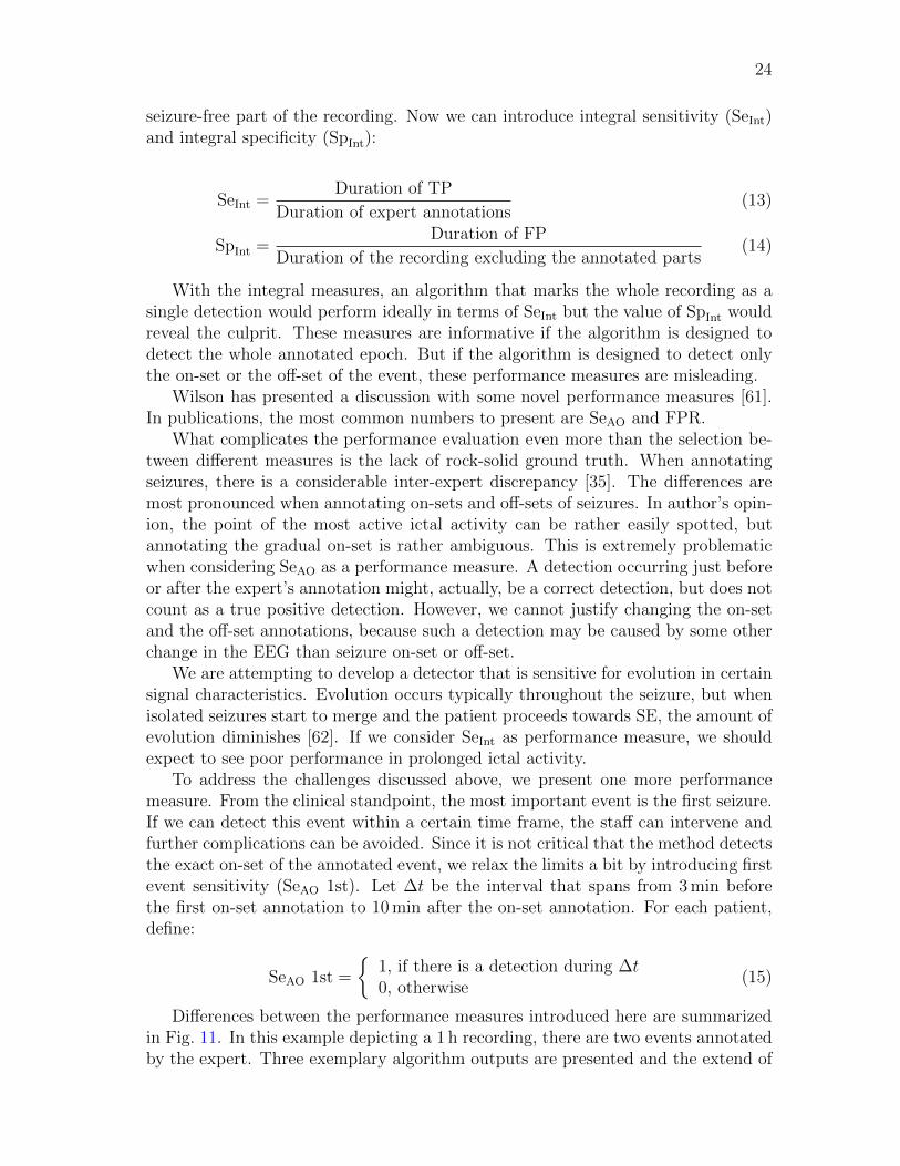
To address the challenges discussed above, we present one more performancemeasure. From the clinical standpoint, the most important event is the first seizure.If we can detect this event within a certain time frame, the staff can intervene andfurther complications can be avoided. Since it is not critical that the method detectsthe exact on-set of the annotated event, we relax the limits a bit by introducing firstevent sensitivity (SeAO 1st). Let ∆t be the interval that spans from 3min beforethe first on-set annotation to 10min after the on-set annotation. For each patient,define:

SeAO 1st =

�1, if there is a detection during ∆t0, otherwise

(15)

Differences between the performance measures introduced here are summarizedin Fig. 11. In this example depicting a 1 h recording, there are two events annotatedby the expert. Three exemplary algorithm outputs are presented and the extend of

25

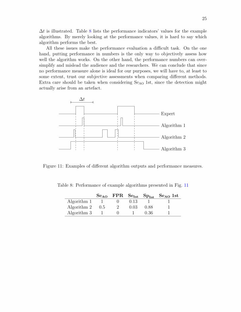
∆t is illustrated. Table 8 lists the performance indicators’ values for the examplealgorithms. By merely looking at the performance values, it is hard to say whichalgorithm performs the best.

All these issues make the performance evaluation a difficult task. On the onehand, putting performance in numbers is the only way to objectively assess howwell the algorithm works. On the other hand, the performance numbers can over-simplify and mislead the audience and the researchers. We can conclude that sinceno performance measure alone is ideal for our purposes, we will have to, at least tosome extent, trust our subjective assessments when comparing different methods.Extra care should be taken when considering SeAO 1st, since the detection mightactually arise from an artefact.

Expert

∆t

Algorithm 1

Algorithm 2

Algorithm 3

Figure 11: Examples of different algorithm outputs and performance measures.

Table 8: Performance of example algorithms presented in Fig. 11

SeAO FPR SeInt SpInt SeAO 1st

Algorithm 1 1 0 0.13 1 1Algorithm 2 0.5 2 0.03 0.88 1Algorithm 3 1 0 1 0.36 1

26

4 EEG feature space

4.1 EEG preprocessing

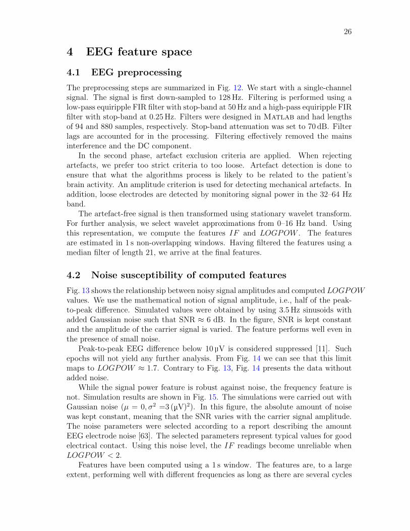
The preprocessing steps are summarized in Fig. 12. We start with a single-channelsignal. The signal is first down-sampled to 128Hz. Filtering is performed using alow-pass equiripple FIR filter with stop-band at 50Hz and a high-pass equiripple FIRfilter with stop-band at 0.25Hz. Filters were designed in Matlab and had lengthsof 94 and 880 samples, respectively. Stop-band attenuation was set to 70 dB. Filterlags are accounted for in the processing. Filtering effectively removed the mainsinterference and the DC component.

In the second phase, artefact exclusion criteria are applied. When rejectingartefacts, we prefer too strict criteria to too loose. Artefact detection is done toensure that what the algorithms process is likely to be related to the patient’sbrain activity. An amplitude criterion is used for detecting mechanical artefacts. Inaddition, loose electrodes are detected by monitoring signal power in the 32–64 Hzband.

The artefact-free signal is then transformed using stationary wavelet transform.For further analysis, we select wavelet approximations from 0–16 Hz band. Usingthis representation, we compute the features IF and LOGPOW . The featuresare estimated in 1 s non-overlapping windows. Having filtered the features using amedian filter of length 21, we arrive at the final features.

4.2 Noise susceptibility of computed features

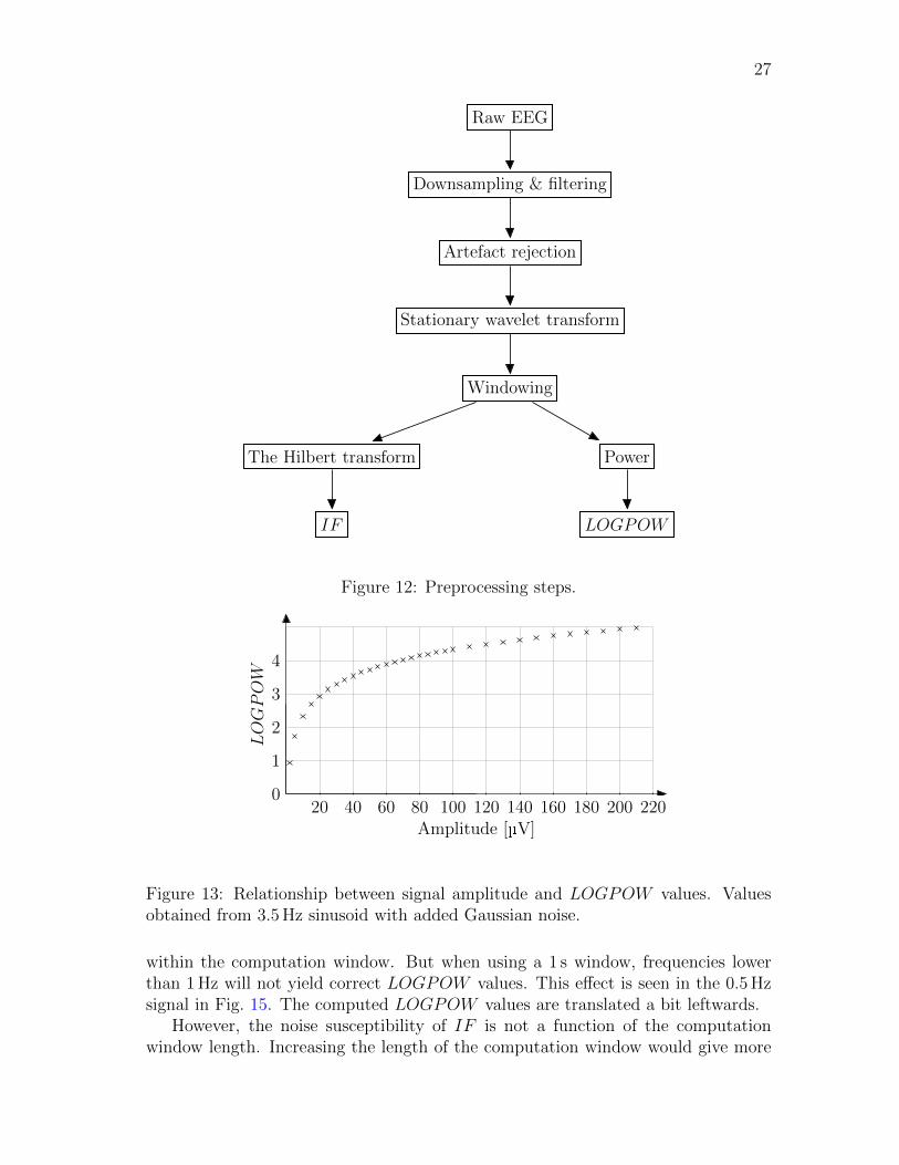
Fig. 13 shows the relationship between noisy signal amplitudes and computed LOGPOWvalues. We use the mathematical notion of signal amplitude, i.e., half of the peak-to-peak difference. Simulated values were obtained by using 3.5Hz sinusoids withadded Gaussian noise such that SNR ≈ 6 dB. In the figure, SNR is kept constantand the amplitude of the carrier signal is varied. The feature performs well even inthe presence of small noise.

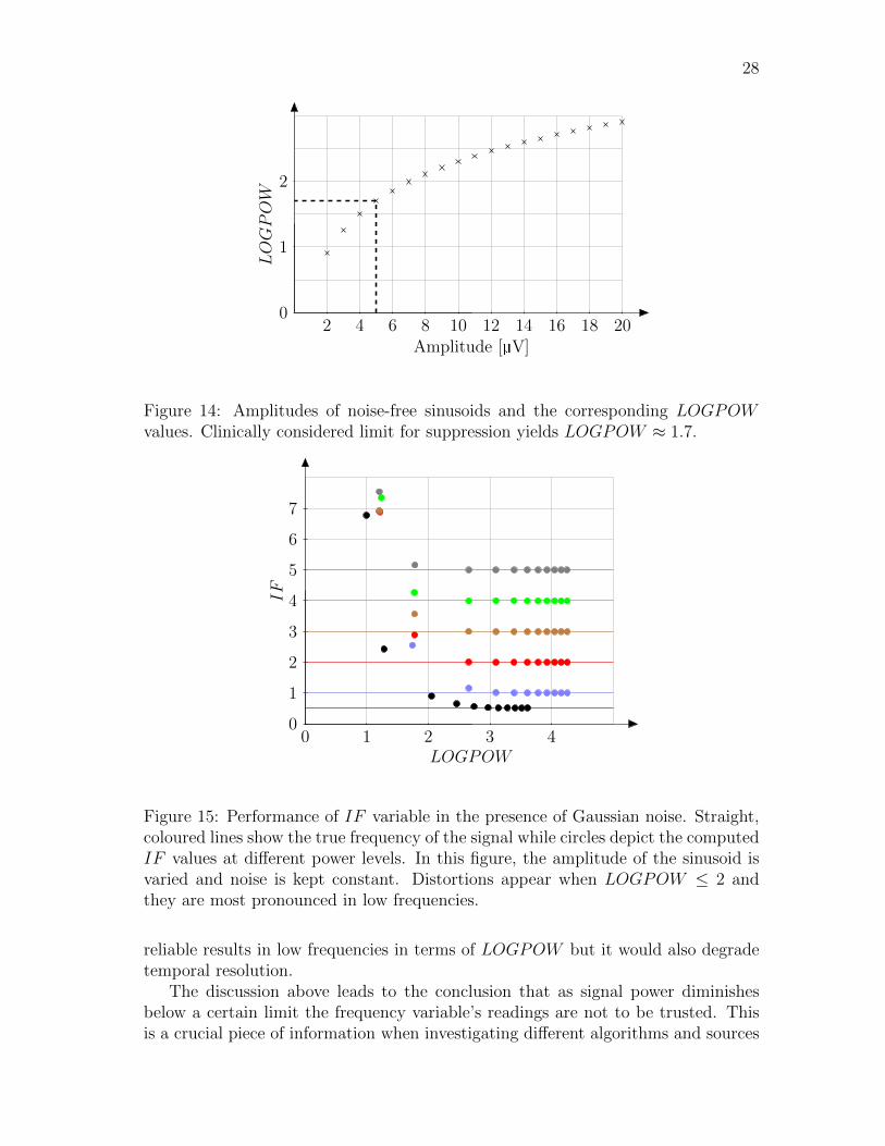
Peak-to-peak EEG difference below 10 V is considered suppressed [11]. Suchepochs will not yield any further analysis. From Fig. 14 we can see that this limitmaps to LOGPOW ≈ 1.7. Contrary to Fig. 13, Fig. 14 presents the data withoutadded noise.

While the signal power feature is robust against noise, the frequency feature isnot. Simulation results are shown in Fig. 15. The simulations were carried out withGaussian noise (µ = 0, σ2 =3 ( V)2). In this figure, the absolute amount of noisewas kept constant, meaning that the SNR varies with the carrier signal amplitude.The noise parameters were selected according to a report describing the amountEEG electrode noise [63]. The selected parameters represent typical values for goodelectrical contact. Using this noise level, the IF readings become unreliable whenLOGPOW < 2.

Features have been computed using a 1 s window. The features are, to a largeextent, performing well with different frequencies as long as there are several cycles

27

Raw EEG

Downsampling & filtering

Artefact rejection

Stationary wavelet transform

Windowing

The Hilbert transform

IF

Power

LOGPOW

Figure 12: Preprocessing steps.

LOGPOW

Amplitude [ V]20 40 60 80 100 120 140 160 180 200 220

0

1

2

3

4

Figure 13: Relationship between signal amplitude and LOGPOW values. Valuesobtained from 3.5Hz sinusoid with added Gaussian noise.

within the computation window. But when using a 1 s window, frequencies lowerthan 1Hz will not yield correct LOGPOW values. This effect is seen in the 0.5Hzsignal in Fig. 15. The computed LOGPOW values are translated a bit leftwards.

However, the noise susceptibility of IF is not a function of the computationwindow length. Increasing the length of the computation window would give more

28

LOGPOW

Amplitude [ V]2 4 6 8 10 12 14 16 18 20

0

1

2

Figure 14: Amplitudes of noise-free sinusoids and the corresponding LOGPOWvalues. Clinically considered limit for suppression yields LOGPOW ≈ 1.7.

IF

LOGPOW0 1 2 3 4

0

1

2

3

4

5

6

7

Figure 15: Performance of IF variable in the presence of Gaussian noise. Straight,coloured lines show the true frequency of the signal while circles depict the computedIF values at different power levels. In this figure, the amplitude of the sinusoid isvaried and noise is kept constant. Distortions appear when LOGPOW ≤ 2 andthey are most pronounced in low frequencies.

reliable results in low frequencies in terms of LOGPOW but it would also degradetemporal resolution.

The discussion above leads to the conclusion that as signal power diminishesbelow a certain limit the frequency variable’s readings are not to be trusted. Thisis a crucial piece of information when investigating different algorithms and sources

29

of their possible shortcomings. The clinical limit of EEG suppression and the lowerbound of signal power that yields reliable frequency estimates are, luckily, almostthe same. When designing the algorithms, we have selected to exclude epochs wherethe feature values might not be reliable and EEG is close to the limit of suppression.At this stage the exclusion is based on binary logics. If EEG is close to the limitof suppression, this causes unwanted jumps in feature values. A more sophisticatedway to handle EEG that is close to the suppression limit would be to design a splinethat would make the transition smooth.

Low-frequency signals are more susceptible to noise than high-frequency signals.This is mostly due to the windowing parameters we selected. It is a widely appre-ciated fact that low-frequency signals need more samples for reliable analysis thanhigh-frequency signals. One way to treat different frequencies equally would be toconsider the amount of cycles in the computation window.

4.3 Prototype seizure

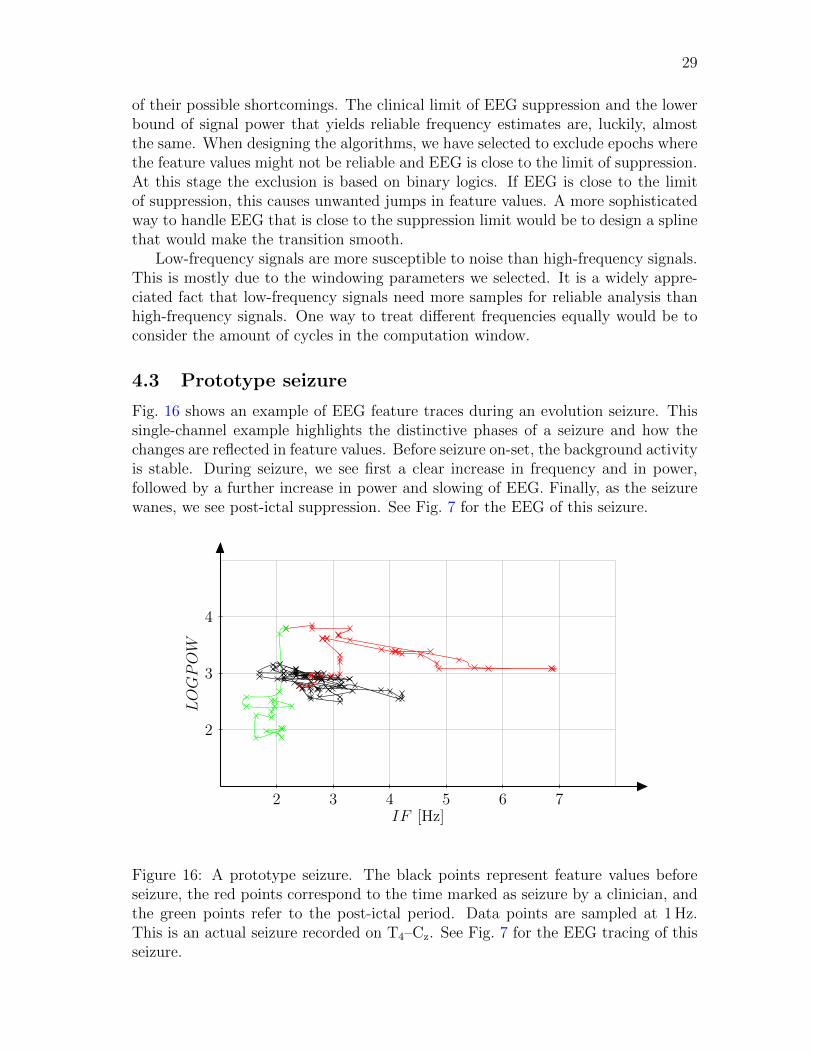
Fig. 16 shows an example of EEG feature traces during an evolution seizure. Thissingle-channel example highlights the distinctive phases of a seizure and how thechanges are reflected in feature values. Before seizure on-set, the background activityis stable. During seizure, we see first a clear increase in frequency and in power,followed by a further increase in power and slowing of EEG. Finally, as the seizurewanes, we see post-ictal suppression. See Fig. 7 for the EEG of this seizure.

IF [Hz]

LOGPOW

2 3 4 5 6 7

2

3

4

Figure 16: A prototype seizure. The black points represent feature values beforeseizure, the red points correspond to the time marked as seizure by a clinician, andthe green points refer to the post-ictal period. Data points are sampled at 1Hz.This is an actual seizure recorded on T4–Cz. See Fig. 7 for the EEG tracing of thisseizure.

30

We will use this prototype seizure to show how different algorithms approachthe problem of detecting seizure-related evolution. It should be noted that whilethis example seems like an easy one to be detected, seizures in reality come in allshapes and sizes. This example is used merely for illustration purposes and by nomeans represents a template. Finally, it should be noted that even though we usesingle-channel data for visualization here, the algorithms process multichannel data,allowing for comparisons between brain regions.

It is insightful to pay attention to how the specialist has annotated the seizure.Feature values at the on-set cannot be distinguished from the background, butthe expert has already seen ictal patterns. In striking difference with automateddetection systems, specialists often review data rewinding forward and backward.This allows them to spot the most easily detectable phase of seizure and then torewind back to fine-comb the channels to find the first indications. Same applies forthe end mark. Automated systems, however, should make annotations in real time,without the possibility of returning back in time. For this reason, trying to optimizethe system to follow specialist’s annotations too strictly may not be a reasonablegoal for the development project.

31

5 Developed algorithms

This section describes the algorithms that were developed in the course of thisthesis. Three algorithms were developed using a slightly different rationale in eachcase. The three proposed algorithms use the same EEG features.

5.1 Algorithm I: Path length

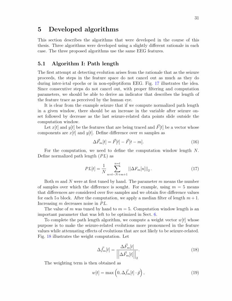
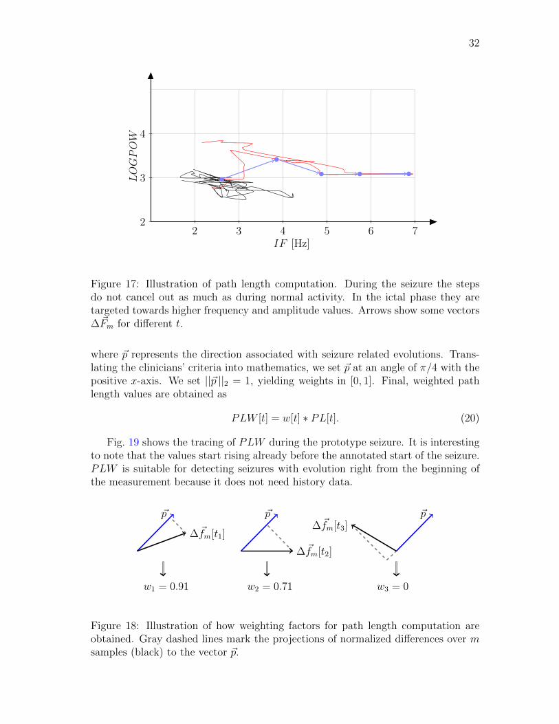
The first attempt at detecting evolution arises from the rationale that as the seizureproceeds, the steps in the feature space do not cancel out as much as they doduring inter-ictal epochs or in non-epileptiform EEG. Fig. 17 illustrates the idea.Since consecutive steps do not cancel out, with proper filtering and computationparameters, we should be able to derive an indicator that describes the length ofthe feature trace as perceived by the human eye.

It is clear from the example seizure that if we compute normalized path lengthin a given window, there should be an increase in the variable after seizure on-set followed by decrease as the last seizure-related data points slide outside thecomputation window.

Let x[t] and y[t] be the features that are being traced and �F [t] be a vector whosecomponents are x[t] and y[t]. Define difference over m samples as

∆�Fm[t] = �F [t]− �F [t−m]. (16)

For the computation, we need to define the computation window length N .Define normalized path length (PL) as

PL[t] =1

N

n=t�

n=t−N+m+1

||∆Fm[n]||2 . (17)

Both m and N were at first tuned by hand. The parameter m means the numberof samples over which the difference is sought. For example, using m = 5 meansthat differences are considered over five samples and we obtain five difference valuesfor each 5 s block. After the computation, we apply a median filter of length m+1.Increasing m decreases noise in PL.

The value of m was tuned by hand to m = 5. Computation window length is animportant parameter that was left to be optimized in Sect. 6.

To complete the path length algorithm, we compute a weight vector w[t] whosepurpose is to make the seizure-related evolutions more pronounced in the featurevalues while attenuating effects of evolutions that are not likely to be seizure-related.Fig. 18 illustrates the weight computation. Let

∆�fm[t] =∆�Fm[t]���

���∆�Fm[t]������2

. (18)

The weighting term is then obtained as

w[t] = max�0,∆�fm[t] · �p

�, (19)

32

LOGPOW

IF [Hz]2 3 4 5 6 7

2

3

4

Figure 17: Illustration of path length computation. During the seizure the stepsdo not cancel out as much as during normal activity. In the ictal phase they aretargeted towards higher frequency and amplitude values. Arrows show some vectors∆�Fm for different t.

where �p represents the direction associated with seizure related evolutions. Trans-lating the clinicians’ criteria into mathematics, we set �p at an angle of π/4 with thepositive x-axis. We set ||�p ||2 = 1, yielding weights in [0, 1]. Final, weighted pathlength values are obtained as

PLW [t] = w[t] ∗ PL[t]. (20)

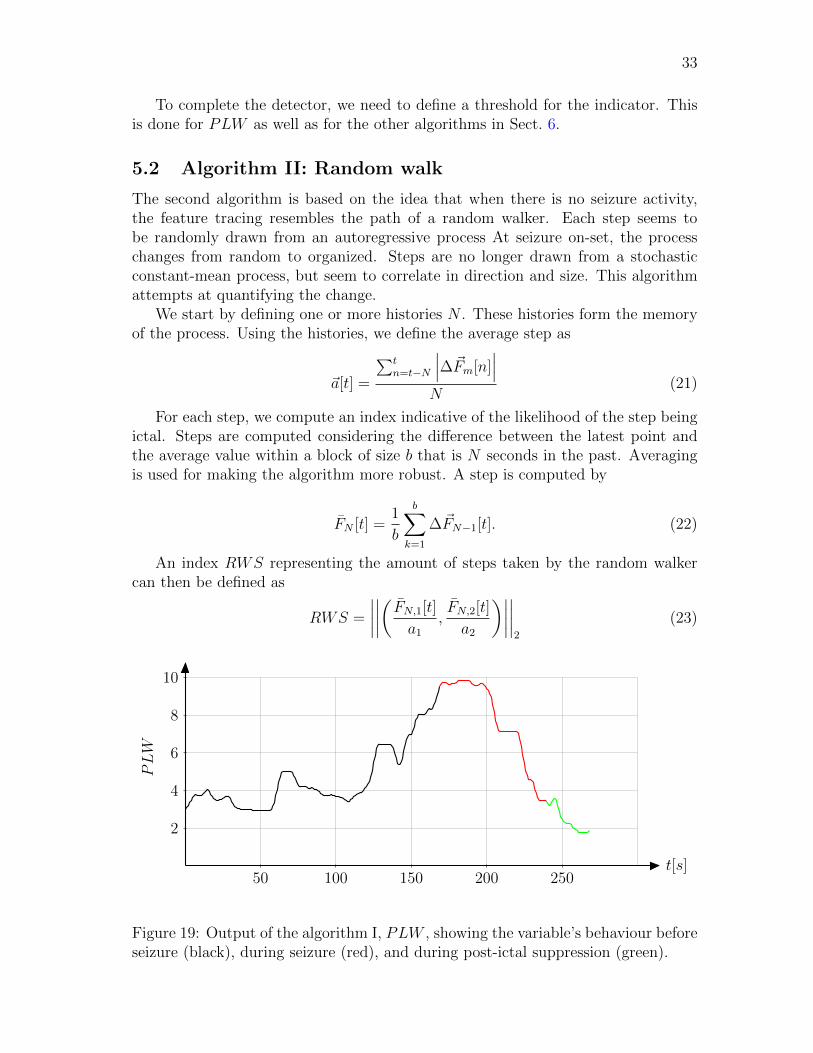
Fig. 19 shows the tracing of PLW during the prototype seizure. It is interestingto note that the values start rising already before the annotated start of the seizure.PLW is suitable for detecting seizures with evolution right from the beginning ofthe measurement because it does not need history data.

∆�fm[t1]

�p

w1 = 0.91

∆�fm[t2]

�p

w2 = 0.71

∆�fm[t3]�p

w3 = 0

Figure 18: Illustration of how weighting factors for path length computation areobtained. Gray dashed lines mark the projections of normalized differences over msamples (black) to the vector �p.

33

To complete the detector, we need to define a threshold for the indicator. Thisis done for PLW as well as for the other algorithms in Sect. 6.

5.2 Algorithm II: Random walk

The second algorithm is based on the idea that when there is no seizure activity,the feature tracing resembles the path of a random walker. Each step seems tobe randomly drawn from an autoregressive process At seizure on-set, the processchanges from random to organized. Steps are no longer drawn from a stochasticconstant-mean process, but seem to correlate in direction and size. This algorithmattempts at quantifying the change.

We start by defining one or more histories N . These histories form the memoryof the process. Using the histories, we define the average step as

�a[t] =

�tn=t−N

���∆�Fm[n]���

N(21)

For each step, we compute an index indicative of the likelihood of the step beingictal. Steps are computed considering the difference between the latest point andthe average value within a block of size b that is N seconds in the past. Averagingis used for making the algorithm more robust. A step is computed by

FN [t] =1

b

b�

k=1

∆�FN−1[t]. (22)

An index RWS representing the amount of steps taken by the random walkercan then be defined as

RWS =

����

����

�FN,1[t]

a1,FN,2[t]

a2

�����

����2

(23)

t[s]50 100 150 200 250

2

4

6

8

10

PLW

Figure 19: Output of the algorithm I, PLW , showing the variable’s behaviour beforeseizure (black), during seizure (red), and during post-ictal suppression (green).

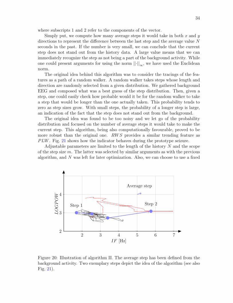
34

where subscripts 1 and 2 refer to the components of the vector.Simply put, we compute how many average steps it would take in both x and y

directions to represent the difference between the last step and the average value Nseconds in the past. If the number is very small, we can conclude that the currentstep does not stand out from the history data. A large value means that we canimmediately recognize the step as not being a part of the background activity. Whileone could present arguments for using the norm ||·||∞, we have used the Euclideannorm.

The original idea behind this algorithm was to consider the tracings of the fea-tures as a path of a random walker. A random walker takes steps whose length anddirection are randomly selected from a given distribution. We gathered backgroundEEG and composed what was a best guess of the step distribution. Then, given astep, one could easily check how probable would it be for the random walker to takea step that would be longer than the one actually taken. This probability tends tozero as step sizes grow. With small steps, the probability of a longer step is large,an indication of the fact that the step does not stand out from the background.

The original idea was found to be too noisy and we let go of the probabilitydistribution and focused on the number of average steps it would take to make thecurrent step. This algorithm, being also computationally favourable, proved to bemore robust than the original one. RWS provides a similar trending feature asPLW . Fig. 21 shows how the indicator behaves during the prototype seizure.

Adjustable parameters are limited to the length of the history N and the scopeof the step size m. The latter was selected by similar arguments as with the previousalgorithm, and N was left for later optimization. Also, we can choose to use a fixed

LOGPOW

IF [Hz]2 3 4 5 6 7

2

3

4

Average step

Step 1 Step 2

Figure 20: Illustration of algorithm II. The average step has been defined from thebackground activity. Two exemplary steps depict the idea of the algorithm (see alsoFig. 21).

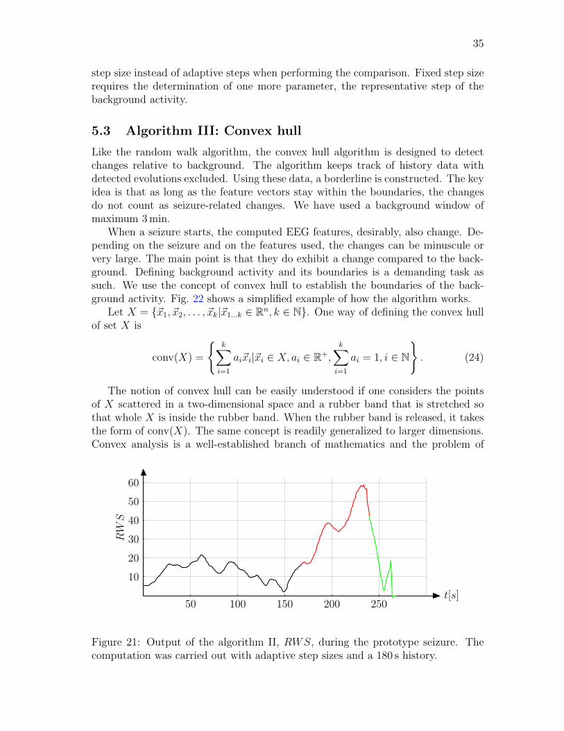
35

step size instead of adaptive steps when performing the comparison. Fixed step sizerequires the determination of one more parameter, the representative step of thebackground activity.

5.3 Algorithm III: Convex hull

Like the random walk algorithm, the convex hull algorithm is designed to detectchanges relative to background. The algorithm keeps track of history data withdetected evolutions excluded. Using these data, a borderline is constructed. The keyidea is that as long as the feature vectors stay within the boundaries, the changesdo not count as seizure-related changes. We have used a background window ofmaximum 3min.

When a seizure starts, the computed EEG features, desirably, also change. De-pending on the seizure and on the features used, the changes can be minuscule orvery large. The main point is that they do exhibit a change compared to the back-ground. Defining background activity and its boundaries is a demanding task assuch. We use the concept of convex hull to establish the boundaries of the back-ground activity. Fig. 22 shows a simplified example of how the algorithm works.

Let X = {�x1, �x2, . . . , �xk|�x1...k ∈ Rn, k ∈ N}. One way of defining the convex hullof set X is

conv(X) =

�k�

i=1

ai�xi|�xi ∈ X, ai ∈ R+,k�

i=1

ai = 1, i ∈ N�. (24)

The notion of convex hull can be easily understood if one considers the pointsof X scattered in a two-dimensional space and a rubber band that is stretched sothat whole X is inside the rubber band. When the rubber band is released, it takesthe form of conv(X). The same concept is readily generalized to larger dimensions.Convex analysis is a well-established branch of mathematics and the problem of

t[s]50 100 150 200 250

10

20

30

40

50

60

RW

S

Figure 21: Output of the algorithm II, RWS, during the prototype seizure. Thecomputation was carried out with adaptive step sizes and a 180 s history.

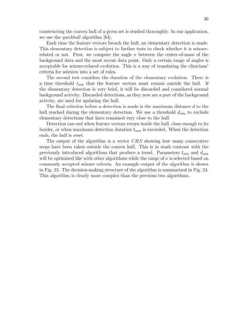
36

constructing the convex hull of a given set is studied thoroughly. In our application,we use the quickhull algorithm [64].

Each time the feature vectors breach the hull, an elementary detection is made.This elementary detection is subject to further tests to check whether it is seizure-related or not. First, we compute the angle ν between the center-of-mass of thebackground data and the most recent data point. Only a certain range of angles isacceptable for seizure-related evolution. This is a way of translating the clinicians’criteria for seizures into a set of rules.

The second test considers the duration of the elementary evolution. There isa time threshold tmin that the feature vectors must remain outside the hull. Ifthe elementary detection is very brief, it will be discarded and considered normalbackground activity. Discarded detections, as they now are a part of the backgroundactivity, are used for updating the hull.

The final criterion before a detection is made is the maximum distance d to thehull reached during the elementary detection. We use a threshold dmin to excludeelementary detections that have remained very close to the hull.

Detection can end when feature vectors return inside the hull, close enough to itsborder, or when maximum detection duration tmax is exceeded. When the detectionends, the hull is reset.

The output of the algorithm is a vector CHS showing how many consecutivesteps have been taken outside the convex hull. This is in stark contrast with thepreviously introduced algorithms that produce a trend. Parameters tmin and dmin

will be optimized like with other algorithms while the range of ν is selected based oncommonly accepted seizure criteria. An example output of the algorithm is shownin Fig. 23. The decision-making structure of the algorithm is summarized in Fig. 24.This algorithm is clearly more complex than the previous two algorithms.

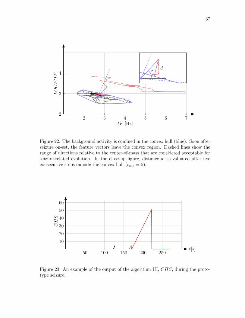
37

LOGPOW

IF [Hz]2 3 4 5 6 7

2

3

4ν d

Figure 22: The background activity is confined in the convex hull (blue). Soon afterseizure on-set, the feature vectors leave the convex region. Dashed lines show therange of directions relative to the center-of-mass that are considered acceptable forseizure-related evolution. In the close-up figure, distance d is evaluated after fiveconsecutive steps outside the convex hull (tmin = 5).

t[s]50 100 150 200 250

10

20

30

40

50

60

CHS

Figure 23: An example of the output of the algorithm III, CHS, during the proto-type seizure.

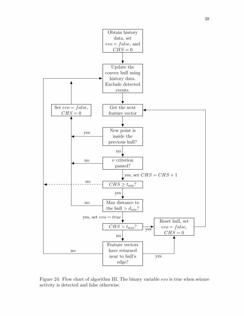
38

Obtain historydata, set

evo = false, andCHS = 0

Update theconvex hull usinghistory data.

Exclude detectedevents.

Get the nextfeature vector

New point isinside the

previous hull?

ν criterionpassed?

CHS ≥ tmin?

Max distance tothe hull > dmin?

CHS > tmax?Reset hull, setevo = false,CHS = 0

Feature vectorshave returnednear to hull’s

edge?

Set evo = false,CHS = 0

no

yes

yes, set CHS = CHS + 1

no

yes

no

yes, set evo = true

no

yes

no

noyes

Figure 24: Flow chart of algorithm III. The binary variable evo is true when seizureactivity is detected and false otherwise.

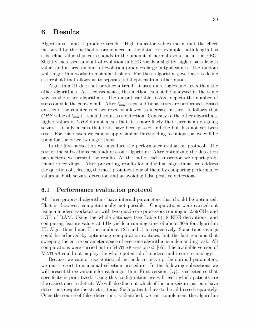
39

6 Results

Algorithms I and II produce trends. High indicator values mean that the effectmeasured by the method is pronounced in the data. For example, path length hasa baseline value that corresponds to the amount of normal evolution in the EEG.Slightly increased amount of evolution in EEG yields a slightly higher path lengthvalue, and a large amount of evolution produces large output values. The randomwalk algorithm works in a similar fashion. For these algorithms, we have to definea threshold that allows us to separate ictal epochs from other data.

Algorithm III does not produce a trend. It uses more logics and tests than theother algorithms. As a consequence, this method cannot be analysed in the sameway as the other algorithms. The output variable, CHS, depicts the number ofsteps outside the convex hull. After tmin steps additional tests are performed. Basedon them, the counter is either reset or allowed to increase further. It follows thatCHS value of tmin+1 should count as a detection. Contrary to the other algorithms,higher values of CHS do not mean that it is more likely that there is an on-goingseizure. It only means that tests have been passed and the hull has not yet beenreset. For this reason we cannot apply similar thresholding techniques as we will beusing for the other two algorithms.

In the first subsection we introduce the performance evaluation protocol. Therest of the subsections each address one algorithm. After optimizing the detectionparameters, we present the results. At the end of each subsection we report prob-lematic recordings. After presenting results for individual algorithms, we addressthe question of selecting the most prominent one of them by comparing performancevalues at both seizure detection and at avoiding false positive detections.

6.1 Performance evaluation protocol

All three proposed algorithms have internal parameters that should be optimized.That is, however, computationally not possible. Computations were carried outusing a modern workstation with two quad-core processors running at 2.66GHz and3GB of RAM. Using the whole database (see Table 6), 8 EEG derivations, andcomputing feature values at 1Hz yields a running time of about 30 h for algorithmIII. Algorithms I and II run in about 12 h and 15 h, respectively. Some time savingscould be achieved by optimizing computation routines, but the fact remains thatsweeping the entire parameter space of even one algorithm is a demanding task. Allcomputations were carried out in Matlab version 6.5 [65]. The available version ofMatlab could not employ the whole potential of modern multi-core technology.

Because we cannot use statistical methods to pick up the optimal parameters,we must resort to a manual selection procedure. In the following subsections wewill present three variants for each algorithm. First version, (v1), is selected so thatspecificity is prioritized. Using this configuration, we will learn which patients arethe easiest ones to detect. We will also find out which of the non-seizure patients havedetections despite the strict criteria. Such patients have to be addressed separately.Once the source of false detections is identified, we can complement the algorithm

40

with a routine that detects and excludes such epochs.Second configuration (v2) is designed so that sensitivity of the method is maxi-

mized, while keeping the amount of false detections at a reasonable level. With thisset-up, we can learn which patients are likely remain out of the scope of the method.Again, these patients must be addressed separately, e.g., by spike detector.

Third configuration (v3) is selected between the two extrema. This configurationrepresents a compromise and gives an idea of the realistic potential of the methodat the current development stage. This version is not presented for algorithm IIIbecause of the method’s computational burden.

There is a considerable amount of subjective judging when picking the repre-sentatives of each method. There is no reasonable way to pick the configurationsautomatically. The author has used the same criteria with all methods when select-ing parameter values, but this remains a source of subjectiveness in the study.

We present several performance measures for each algorithm. False positivedetections are reported only for patients with no annotated seizures. FPRw refers tothe duration-weighted average FPR. FPRpa refers to non-weighted patient averages,obtained after pooling all recordings of each patient together. SeAO 1st refers toSeAO when considering relaxed first annotated seizure of the patient (see Fig. 11).Patient sensitivity is 1 for seizure patients that have any detections in SeAO sense.In results, we present the value averaged over all seizure patients (SeAO pt). Wealso report SeAO when all seizures in the database are considered (SeAO all szs), andthe average of patients’ SeAO values (SeAO pt szs). Integral specificities (SpInt) arereported in the same fashion as FPR values. Finally, we report integral sensitivitycomputed over all seizure records (SeInt).

We have to investigate the performance values as whole. Concentrating too muchon a single value can be misleading. The lack of one accepted performance valuecan, unfortunately, introduce a bit of vagueness in the arguments presented below.

6.2 Performance of algorithm I

Since we are not interested in short transients that cause the indicator to rise abovethe threshold, we need to establish a threshold also on the time axis. Based onclinical guidelines, we set the threshold to 10 s. Thus, for a detection to be counted,the indicator value shall exceed the threshold continuously for more than 10 s.

To obtain the three representative versions, we try out several threshold values.We start with v2 using a low threshold. Next, we start gradually rising the threshold.We are looking for a reasonable compromise between FPR and SeAO. The thresholdfor v2 is set at the value from which further increase cannot be achieved withoutsignificantly deteriorating detection capability.

For v1, we continue rising the threshold value until we find a limit that gives de-tections only on the most pronounced seizures. Threshold for v3 is selected betweenthe extrema.

Results obtained using this scheme are summarized in Tables 9 and 10. PL30refers to a 30 s history, PL90 to a 90 s history, PL180 to a 180 s history, and PLAVEto the average of the three. The data show that PLAVE and PL30 are the most

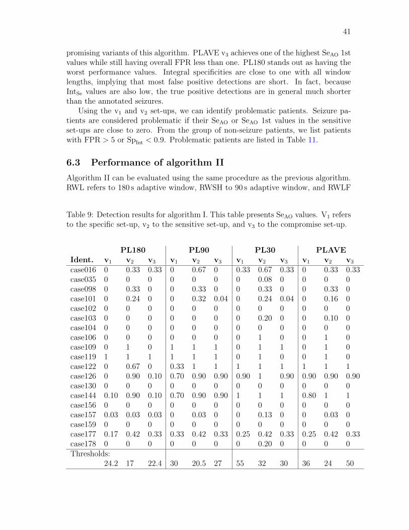
41

promising variants of this algorithm. PLAVE v3 achieves one of the highest SeAO 1stvalues while still having overall FPR less than one. PL180 stands out as having theworst performance values. Integral specificities are close to one with all windowlengths, implying that most false positive detections are short. In fact, becauseIntSe values are also low, the true positive detections are in general much shorterthan the annotated seizures.

Using the v1 and v2 set-ups, we can identify problematic patients. Seizure pa-tients are considered problematic if their SeAO or SeAO 1st values in the sensitiveset-ups are close to zero. From the group of non-seizure patients, we list patientswith FPR > 5 or SpInt < 0.9. Problematic patients are listed in Table 11.

6.3 Performance of algorithm II

Algorithm II can be evaluated using the same procedure as the previous algorithm.RWL refers to 180 s adaptive window, RWSH to 90 s adaptive window, and RWLF

Table 9: Detection results for algorithm I. This table presents SeAO values. V1 refersto the specific set-up, v2 to the sensitive set-up, and v3 to the compromise set-up.

PL180 PL90 PL30 PLAVE

Ident. v1 v2 v3 v1 v2 v3 v1 v2 v3 v1 v2 v3

case016 0 0.33 0.33 0 0.67 0 0.33 0.67 0.33 0 0.33 0.33case035 0 0 0 0 0 0 0 0.08 0 0 0 0case098 0 0.33 0 0 0.33 0 0 0.33 0 0 0.33 0case101 0 0.24 0 0 0.32 0.04 0 0.24 0.04 0 0.16 0case102 0 0 0 0 0 0 0 0 0 0 0 0case103 0 0 0 0 0 0 0 0.20 0 0 0.10 0case104 0 0 0 0 0 0 0 0 0 0 0 0case106 0 0 0 0 0 0 0 1 0 0 1 0case109 0 1 0 1 1 1 0 1 1 0 1 0case119 1 1 1 1 1 1 0 1 0 0 1 0case122 0 0.67 0 0.33 1 1 1 1 1 1 1 1case126 0 0.90 0.10 0.70 0.90 0.90 0.90 1 0.90 0.90 0.90 0.90case130 0 0 0 0 0 0 0 0 0 0 0 0case144 0.10 0.90 0.10 0.70 0.90 0.90 1 1 1 0.80 1 1case156 0 0 0 0 0 0 0 0 0 0 0 0case157 0.03 0.03 0.03 0 0.03 0 0 0.13 0 0 0.03 0case159 0 0 0 0 0 0 0 0 0 0 0 0case177 0.17 0.42 0.33 0.33 0.42 0.33 0.25 0.42 0.33 0.25 0.42 0.33case178 0 0 0 0 0 0 0 0.20 0 0 0 0Thresholds:

24.2 17 22.4 30 20.5 27 55 32 30 36 24 50

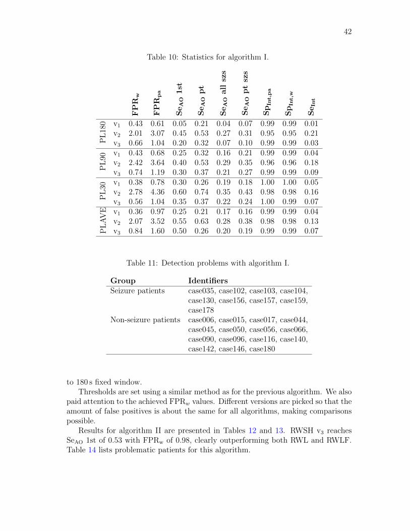
42

Table 10: Statistics for algorithm I.

SeAOall

szs

SeAOptszs

SeAO1st

SeAOpt

SpInt,p

a

SpInt,w

FPR

w

FPR

pa

SeInt

PL180 v1 0.43 0.61 0.05 0.21 0.04 0.07 0.99 0.99 0.01

v2 2.01 3.07 0.45 0.53 0.27 0.31 0.95 0.95 0.21v3 0.66 1.04 0.20 0.32 0.07 0.10 0.99 0.99 0.03

PL90

v1 0.43 0.68 0.25 0.32 0.16 0.21 0.99 0.99 0.04v2 2.42 3.64 0.40 0.53 0.29 0.35 0.96 0.96 0.18v3 0.74 1.19 0.30 0.37 0.21 0.27 0.99 0.99 0.09

PL30

v1 0.38 0.78 0.30 0.26 0.19 0.18 1.00 1.00 0.05v2 2.78 4.36 0.60 0.74 0.35 0.43 0.98 0.98 0.16v3 0.56 1.04 0.35 0.37 0.22 0.24 1.00 0.99 0.07

PLAVE v1 0.36 0.97 0.25 0.21 0.17 0.16 0.99 0.99 0.04

v2 2.07 3.52 0.55 0.63 0.28 0.38 0.98 0.98 0.13v3 0.84 1.60 0.50 0.26 0.20 0.19 0.99 0.99 0.07

Table 11: Detection problems with algorithm I.

Group Identifiers

Seizure patients case035, case102, case103, case104,case130, case156, case157, case159,case178

Non-seizure patients case006, case015, case017, case044,case045, case050, case056, case066,case090, case096, case116, case140,case142, case146, case180

to 180 s fixed window.Thresholds are set using a similar method as for the previous algorithm. We also

paid attention to the achieved FPRw values. Different versions are picked so that theamount of false positives is about the same for all algorithms, making comparisonspossible.

Results for algorithm II are presented in Tables 12 and 13. RWSH v3 reachesSeAO 1st of 0.53 with FPRw of 0.98, clearly outperforming both RWL and RWLF.Table 14 lists problematic patients for this algorithm.

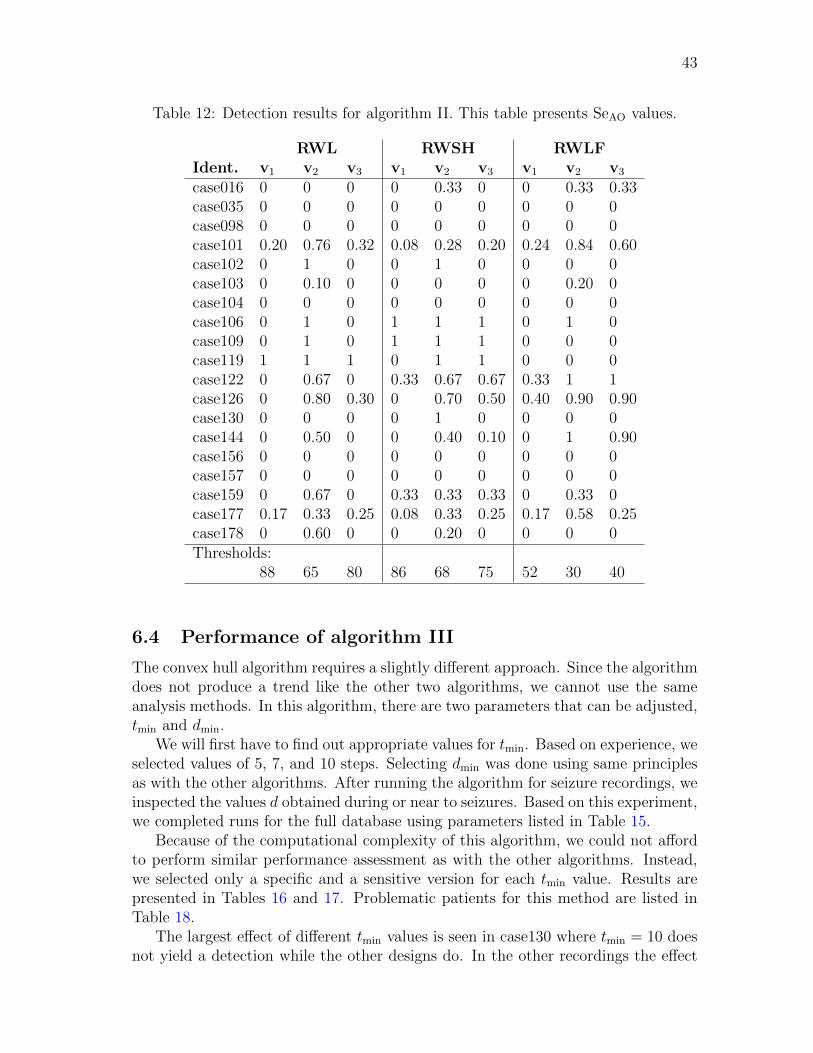
43

Table 12: Detection results for algorithm II. This table presents SeAO values.

RWL RWSH RWLF

Ident. v1 v2 v3 v1 v2 v3 v1 v2 v3

case016 0 0 0 0 0.33 0 0 0.33 0.33case035 0 0 0 0 0 0 0 0 0case098 0 0 0 0 0 0 0 0 0case101 0.20 0.76 0.32 0.08 0.28 0.20 0.24 0.84 0.60case102 0 1 0 0 1 0 0 0 0case103 0 0.10 0 0 0 0 0 0.20 0case104 0 0 0 0 0 0 0 0 0case106 0 1 0 1 1 1 0 1 0case109 0 1 0 1 1 1 0 0 0case119 1 1 1 0 1 1 0 0 0case122 0 0.67 0 0.33 0.67 0.67 0.33 1 1case126 0 0.80 0.30 0 0.70 0.50 0.40 0.90 0.90case130 0 0 0 0 1 0 0 0 0case144 0 0.50 0 0 0.40 0.10 0 1 0.90case156 0 0 0 0 0 0 0 0 0case157 0 0 0 0 0 0 0 0 0case159 0 0.67 0 0.33 0.33 0.33 0 0.33 0case177 0.17 0.33 0.25 0.08 0.33 0.25 0.17 0.58 0.25case178 0 0.60 0 0 0.20 0 0 0 0Thresholds:

88 65 80 86 68 75 52 30 40

6.4 Performance of algorithm III

The convex hull algorithm requires a slightly different approach. Since the algorithmdoes not produce a trend like the other two algorithms, we cannot use the sameanalysis methods. In this algorithm, there are two parameters that can be adjusted,tmin and dmin.

We will first have to find out appropriate values for tmin. Based on experience, weselected values of 5, 7, and 10 steps. Selecting dmin was done using same principlesas with the other algorithms. After running the algorithm for seizure recordings, weinspected the values d obtained during or near to seizures. Based on this experiment,we completed runs for the full database using parameters listed in Table 15.

Because of the computational complexity of this algorithm, we could not affordto perform similar performance assessment as with the other algorithms. Instead,we selected only a specific and a sensitive version for each tmin value. Results arepresented in Tables 16 and 17. Problematic patients for this method are listed inTable 18.

The largest effect of different tmin values is seen in case130 where tmin = 10 doesnot yield a detection while the other designs do. In the other recordings the effect

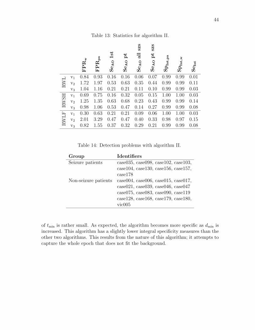
44

Table 13: Statistics for algorithm II.

SeAOall

szs

SeAOptszs

SeAO1st

SeAOpt

SpInt,p

a

SpInt,w

FPR

w

FPR

pa

SeInt

RW

L v1 0.84 0.93 0.16 0.16 0.06 0.07 0.99 0.99 0.01v2 1.72 1.97 0.53 0.63 0.35 0.44 0.99 0.99 0.11v3 1.04 1.16 0.21 0.21 0.11 0.10 0.99 0.99 0.03

RW

SH v1 0.69 0.75 0.16 0.32 0.05 0.15 1.00 1.00 0.03

v2 1.25 1.35 0.63 0.68 0.23 0.43 0.99 0.99 0.14v3 0.98 1.06 0.53 0.47 0.14 0.27 0.99 0.99 0.08

RW

LF v1 0.30 0.63 0.21 0.21 0.09 0.06 1.00 1.00 0.03

v2 2.01 3.29 0.47 0.47 0.40 0.33 0.98 0.97 0.15v3 0.82 1.55 0.37 0.32 0.29 0.21 0.99 0.99 0.08

Table 14: Detection problems with algorithm II.

Group Identifiers

Seizure patients case035, case098, case102, case103,case104, case130, case156, case157,case178

Non-seizure patients case004, case006, case015, case017,case021, case039, case046, case047case075, case083, case090, case119case128, case168, case179, case180,vic005

of tmin is rather small. As expected, the algorithm becomes more specific as dmin isincreased. This algorithm has a slightly lower integral specificity measures than theother two algorithms. This results from the nature of this algorithm; it attempts tocapture the whole epoch that does not fit the background.

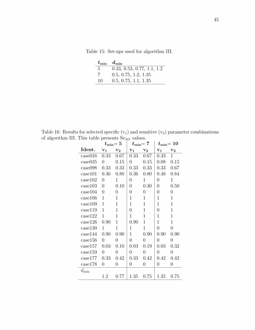
45

Table 15: Set-ups used for algorithm III.

tmin dmin

5 0.33, 0.53, 0.77, 1.1, 1.27 0.5, 0.75, 1.2, 1.3510 0.5, 0.75, 1.1, 1.35

Table 16: Results for selected specific (v1) and sensitive (v2) parameter combinationsof algorithm III. This table presents SeAO values.

tmin= 5 tmin= 7 tmin= 10

Ident. v1 v2 v1 v2 v1 v2

case016 0.33 0.67 0.33 0.67 0.33 1case035 0 0.15 0 0.15 0.08 0.15case098 0.33 0.33 0.33 0.33 0.33 0.67case101 0.36 0.80 0.36 0.80 0.48 0.84case102 0 1 0 1 0 1case103 0 0.10 0 0.30 0 0.50case104 0 0 0 0 0 0case106 1 1 1 1 1 1case109 1 1 1 1 1 1case119 1 1 0 1 0 1case122 1 1 1 1 1 1case126 0.90 1 0.90 1 1 1case130 1 1 1 1 0 0case144 0.90 0.90 1 0.90 0.90 0.90case156 0 0 0 0 0 0case157 0.03 0.10 0.03 0.19 0.03 0.32case159 0 0 0 0 0 0case177 0.33 0.42 0.33 0.42 0.42 0.42case178 0 0 0 0 0 0dmin

1.2 0.77 1.35 0.75 1.35 0.75

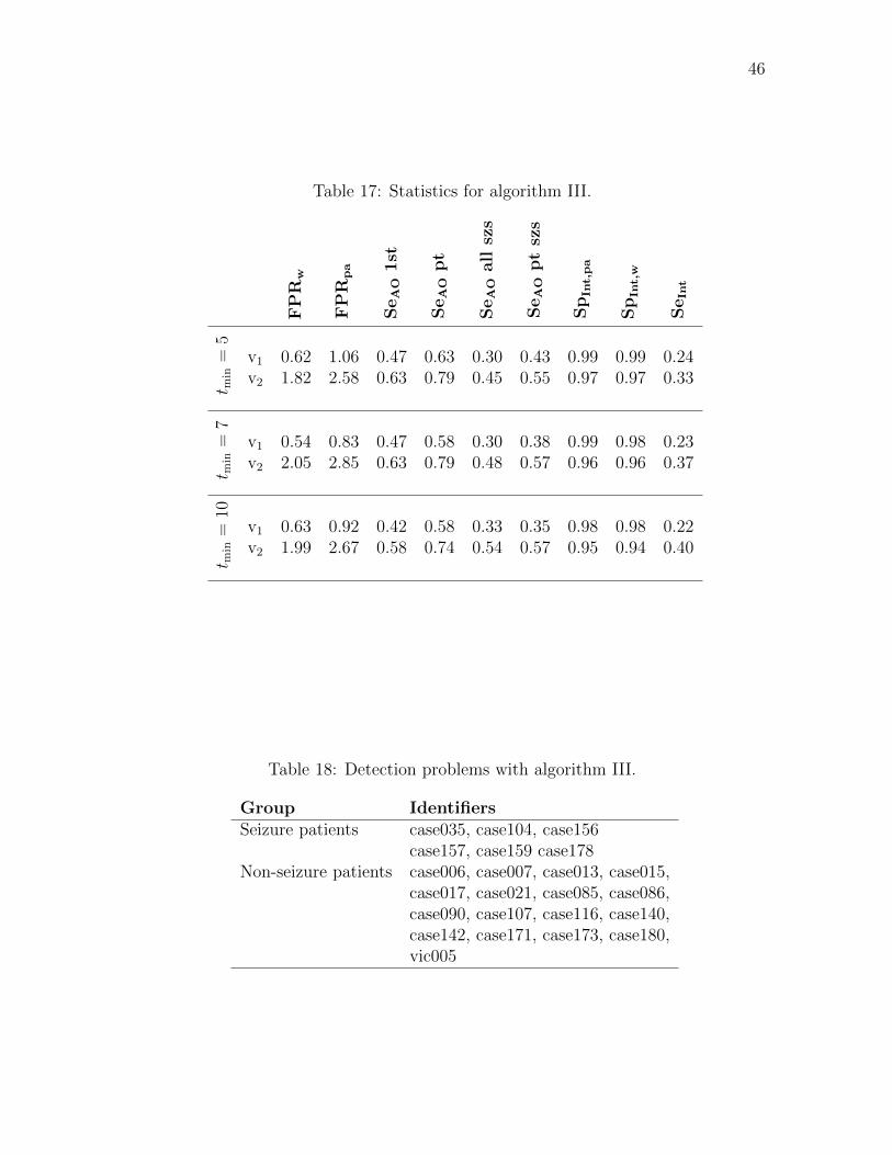
46

Table 17: Statistics for algorithm III.

SeAOall

szs

SeAOptszs

SeAO1st

SeAOpt

SpInt,p

a

SpInt,w

FPR

w

FPR

pa

SeInt

t min=

5

v1 0.62 1.06 0.47 0.63 0.30 0.43 0.99 0.99 0.24v2 1.82 2.58 0.63 0.79 0.45 0.55 0.97 0.97 0.33

t min=

7

v1 0.54 0.83 0.47 0.58 0.30 0.38 0.99 0.98 0.23v2 2.05 2.85 0.63 0.79 0.48 0.57 0.96 0.96 0.37

t min=

10

v1 0.63 0.92 0.42 0.58 0.33 0.35 0.98 0.98 0.22v2 1.99 2.67 0.58 0.74 0.54 0.57 0.95 0.94 0.40

Table 18: Detection problems with algorithm III.

Group Identifiers

Seizure patients case035, case104, case156case157, case159 case178

Non-seizure patients case006, case007, case013, case015,case017, case021, case085, case086,case090, case107, case116, case140,case142, case171, case173, case180,vic005

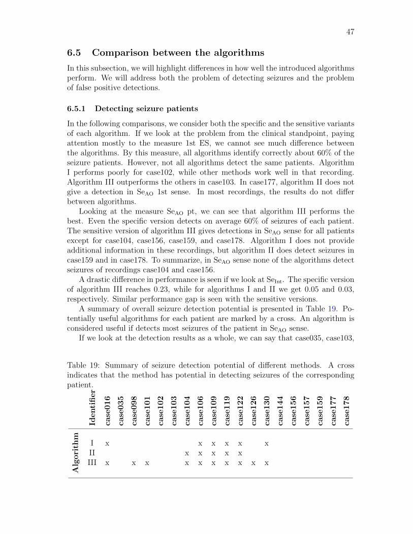
47

6.5 Comparison between the algorithms

In this subsection, we will highlight differences in how well the introduced algorithmsperform. We will address both the problem of detecting seizures and the problemof false positive detections.

6.5.1 Detecting seizure patients

In the following comparisons, we consider both the specific and the sensitive variantsof each algorithm. If we look at the problem from the clinical standpoint, payingattention mostly to the measure 1st ES, we cannot see much difference betweenthe algorithms. By this measure, all algorithms identify correctly about 60% of theseizure patients. However, not all algorithms detect the same patients. AlgorithmI performs poorly for case102, while other methods work well in that recording.Algorithm III outperforms the others in case103. In case177, algorithm II does notgive a detection in SeAO 1st sense. In most recordings, the results do not differbetween algorithms.

Looking at the measure SeAO pt, we can see that algorithm III performs thebest. Even the specific version detects on average 60% of seizures of each patient.The sensitive version of algorithm III gives detections in SeAO sense for all patientsexcept for case104, case156, case159, and case178. Algorithm I does not provideadditional information in these recordings, but algorithm II does detect seizures incase159 and in case178. To summarize, in SeAO sense none of the algorithms detectseizures of recordings case104 and case156.

A drastic difference in performance is seen if we look at SeInt. The specific versionof algorithm III reaches 0.23, while for algorithms I and II we get 0.05 and 0.03,respectively. Similar performance gap is seen with the sensitive versions.

A summary of overall seizure detection potential is presented in Table 19. Po-tentially useful algorithms for each patient are marked by a cross. An algorithm isconsidered useful if detects most seizures of the patient in SeAO sense.

If we look at the detection results as a whole, we can say that case035, case103,

Table 19: Summary of seizure detection potential of different methods. A crossindicates that the method has potential in detecting seizures of the correspondingpatient.

Identifier

case016

case035

case098

case101

case102

case103

case104

case106

case109

case119

case122

case126

case130

case144

case156

case157

case159

case177

case178

Algorithm

I x x x x x xII x x x x xIII x x x x x x x x x x

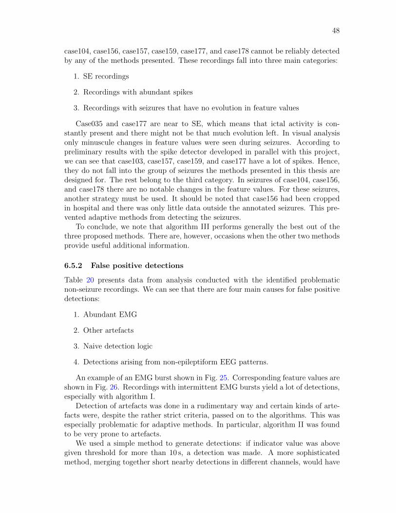
48

case104, case156, case157, case159, case177, and case178 cannot be reliably detectedby any of the methods presented. These recordings fall into three main categories:

1. SE recordings

2. Recordings with abundant spikes

3. Recordings with seizures that have no evolution in feature values

Case035 and case177 are near to SE, which means that ictal activity is con-stantly present and there might not be that much evolution left. In visual analysisonly minuscule changes in feature values were seen during seizures. According topreliminary results with the spike detector developed in parallel with this project,we can see that case103, case157, case159, and case177 have a lot of spikes. Hence,they do not fall into the group of seizures the methods presented in this thesis aredesigned for. The rest belong to the third category. In seizures of case104, case156,and case178 there are no notable changes in the feature values. For these seizures,another strategy must be used. It should be noted that case156 had been croppedin hospital and there was only little data outside the annotated seizures. This pre-vented adaptive methods from detecting the seizures.

To conclude, we note that algorithm III performs generally the best out of thethree proposed methods. There are, however, occasions when the other two methodsprovide useful additional information.

6.5.2 False positive detections

Table 20 presents data from analysis conducted with the identified problematicnon-seizure recordings. We can see that there are four main causes for false positivedetections:

1. Abundant EMG

2. Other artefacts

3. Naive detection logic

4. Detections arising from non-epileptiform EEG patterns.

An example of an EMG burst shown in Fig. 25. Corresponding feature values areshown in Fig. 26. Recordings with intermittent EMG bursts yield a lot of detections,especially with algorithm I.

Detection of artefacts was done in a rudimentary way and certain kinds of arte-facts were, despite the rather strict criteria, passed on to the algorithms. This wasespecially problematic for adaptive methods. In particular, algorithm II was foundto be very prone to artefacts.

We used a simple method to generate detections: if indicator value was abovegiven threshold for more than 10 s, a detection was made. A more sophisticatedmethod, merging together short nearby detections in different channels, would have

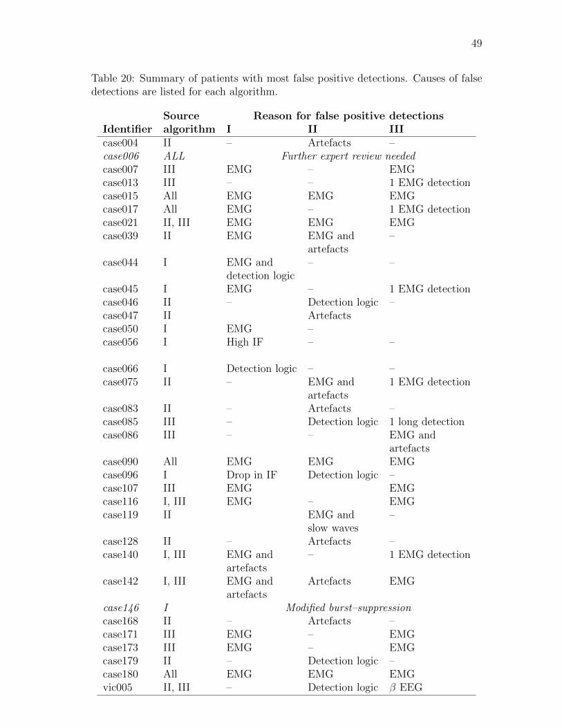
49

Table 20: Summary of patients with most false positive detections. Causes of falsedetections are listed for each algorithm.

Source Reason for false positive detections

Identifier algorithm I II III

case004 II – Artefacts –case006 ALL Further expert review needed

case007 III EMG – EMGcase013 III – – 1 EMG detectioncase015 All EMG EMG EMGcase017 All EMG – 1 EMG detectioncase021 II, III EMG EMG EMGcase039 II EMG EMG and –

artefactscase044 I EMG and – –

detection logiccase045 I EMG – 1 EMG detectioncase046 II – Detection logic –case047 II Artefactscase050 I EMG –case056 I High IF – –

case066 I Detection logic – –case075 II – EMG and 1 EMG detection

artefactscase083 II – Artefacts –case085 III – Detection logic 1 long detectioncase086 III – – EMG and

artefactscase090 All EMG EMG EMGcase096 I Drop in IF Detection logic –case107 III EMG EMGcase116 I, III EMG – EMGcase119 II EMG and –

slow wavescase128 II – Artefacts –case140 I, III EMG and – 1 EMG detection

artefactscase142 I, III EMG and Artefacts EMG

artefactscase146 I Modified burst–suppression

case168 II – Artefacts –case171 III EMG – EMGcase173 III EMG – EMGcase179 II – Detection logic –case180 All EMG EMG EMGvic005 II, III – Detection logic β EEG

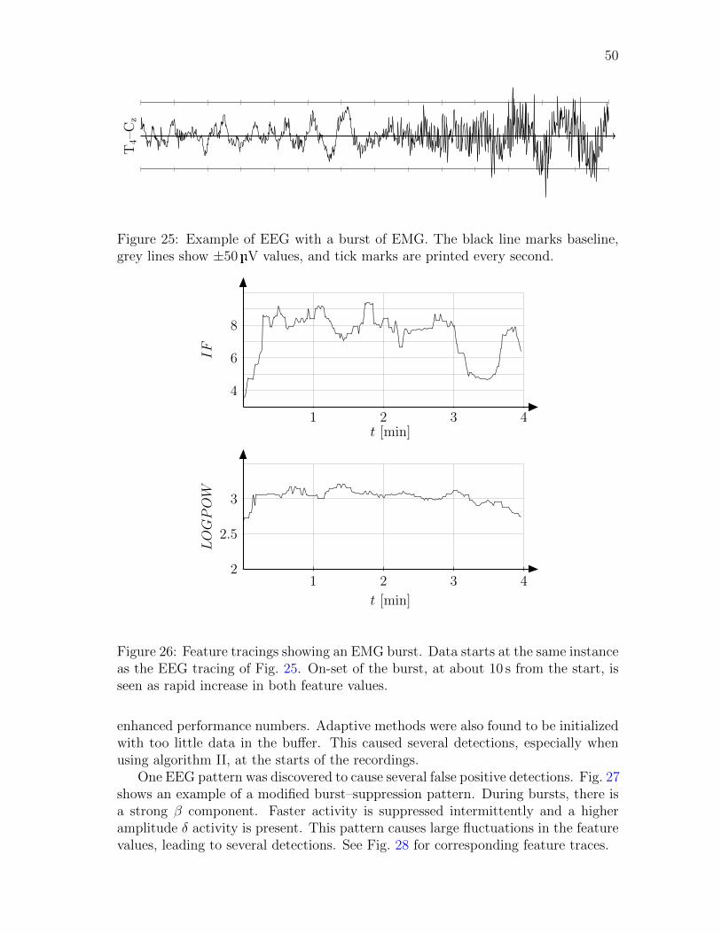
50

T4–C

z

Figure 25: Example of EEG with a burst of EMG. The black line marks baseline,grey lines show ±50 V values, and tick marks are printed every second.

t [min]

IF

1 2 3 4

4

6

8

t [min]

LOGPOW

1 2 3 42

2.5

3

Figure 26: Feature tracings showing an EMG burst. Data starts at the same instanceas the EEG tracing of Fig. 25. On-set of the burst, at about 10 s from the start, isseen as rapid increase in both feature values.

enhanced performance numbers. Adaptive methods were also found to be initializedwith too little data in the buffer. This caused several detections, especially whenusing algorithm II, at the starts of the recordings.

One EEG pattern was discovered to cause several false positive detections. Fig. 27shows an example of a modified burst–suppression pattern. During bursts, there isa strong β component. Faster activity is suppressed intermittently and a higheramplitude δ activity is present. This pattern causes large fluctuations in the featurevalues, leading to several detections. See Fig. 28 for corresponding feature traces.

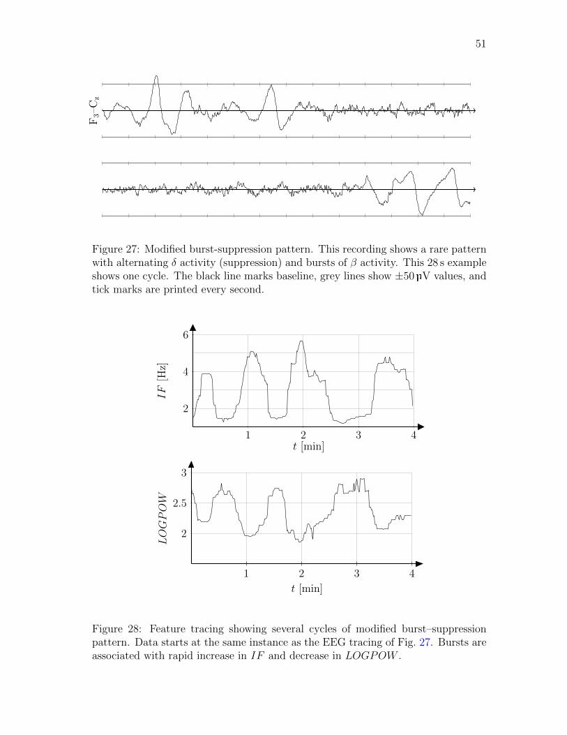
51

F3–C

z

Figure 27: Modified burst-suppression pattern. This recording shows a rare patternwith alternating δ activity (suppression) and bursts of β activity. This 28 s exampleshows one cycle. The black line marks baseline, grey lines show ±50 V values, andtick marks are printed every second.

t [min]

IF[H

z]

1 2 3 4

2

4

6

t [min]

LOGPOW

1 2 3 4

2

2.5

3

Figure 28: Feature tracing showing several cycles of modified burst–suppressionpattern. Data starts at the same instance as the EEG tracing of Fig. 27. Bursts areassociated with rapid increase in IF and decrease in LOGPOW .

52

7 Discussion

The methods presented in this thesis provide a novel way of investigating seizureactivity in EEG. Instead of looking at snapshots of EEG or at absolute values ofsignal features, we approach the problem using the paradigm that in certain casesseizures cause systematic changes in signal properties. Absolute feature values arealso important; most of the current methods use them and they seem to performwell in some patient populations. Our methods focus on dynamic changes in featuretime courses.

During the study, several compromises had to be made. Despite the difficulties,eventually a protocol for assessing the performance of the three proposed methodswas laid out. Analyses conducted in this study mark the way for future research.The proposed methods proved to hold potential for seizure detection.

7.1 Study

Throughout the study we have been cautious about reporting statistical variablesand about drawing conclusions based solely on numbers. This has been an informeddecision. We justify this approach by two arguments.

There is no single widely accepted performance measure for a seizure detectionalgorithm. Some attempts have been made, e.g., by Wilson [61], but in author’sopinion the best overall measure is still escaping the researchers. One factor com-plicating the design of such a measure is the lack of proper specifications. It is easyto define how a perfect algorithm would work, but defining what is rather good orcomparing two almost perfect algorithms is a difficult task. In author’s opinion,the field lacks a common way of reporting results and describing performance. Thisleads to ambiguous reports and difficulties in making comparisons between methods.

Providing a dozen performance measures might be an accurate description ofhow well the algorithm performs, at least for researches with a background in scienceand technology. But we cannot expect medical staff to be specialists in statistics.Designing a widely accepted and simple performance measure might be a utopia butcould also be worth striving for.

Another source of inaccuracy lies in what we consider as the ground truth. Forthis study, we had obtained the opinion of one seasoned expert, Dr. Bryan Young.Even though our consultant is a recognized specialist, we cannot guarantee thatthere are no mistakes in the annotations. And even if there would not be any biggermistakes, another neurologist could have a different opinion regarding the exact on-sets and off-sets of seizures. The best way to overcome this challenge would be toobtain dictations from other specialists and then to combine them. So far this hasbeen limited by resources available for the project, but there are plans to obtainmore dictations from other specialists.

In the presence of these two factors, we decided not to emphasize too much thestatistical numbers and, instead, tried to look at the methods in a more general way.

Statistical optimization methods are very useful when designing algorithms. Inthis study, we wanted to investigate the potential of three proposed algorithms. This

53

led to a situation where we could not afford optimizing any of them in a statisticallysatisfying way. We made an informed decision that it is more useful to try andunderstand the general potential of the proposed methods than to blindly pick oneof them and attempt at tuning it to its full potential.

While the absence of statistical methods could be seen as a scientific shortcom-ing in the study, it has allowed us to gain a more thorough understanding of thecharacteristics of the proposed methods. Such experience is invaluable when takingthe next steps in the development process.

7.2 Characteristics of the designed algorithms

The most intuitive algorithm is the path length algorithm. When evaluating themethod, certain problems were discovered. First and foremost, there were a lotof detections because of EMG. Second problem is that the method is not scale-invariant. In some recordings, we could notice a clear rise in path length valuesduring seizures, proving the idea of the algorithm correct, but the total obtainedpath length values were far too low to yield detections.

Third problem with the path length method was its poor specificity. We wantedto sensitize the method for seizure-related events and added the weighting factor.However, we found some seizures in the database that do show evolution in featurevalues but not in the direction we used. Results could be somewhat different if thedirection of the weighting vector �p was optimized or if a different weighting schemewas implemented.

Overall, the path length algorithm was found to work somewhat well. In mostcases its performance numbers were not as good as those of the other algorithms butit showed consistently acceptable results. The most appealing feature of the pathlength algorithm is its simplicity.

During evolution, the path traced by the features seems be drawn from a deter-ministic process. When there is no seizure activity, the path looks like a collectionof randomly placed edges. The random walk algorithm was designed to quantifythis change. We studied auto-regressive processes and the theory of random walk.Statistical tests were applied to understand if there really was a transition froma random or auto-regressive process to another process at seizure on-set. It wasquickly established that such methods are not robust enough for our applicationand that a new method should be designed.

The random walk algorithm quantifies changes in feature values rather well. Likethe path length algorithm, it produces a trend. The output value is proportional tothe amount how much the current step differs from the past steps.

In the analyses reported here, we have seen that this method has a rather goodperformance. In several cases it seems to outperform the path length algorithm.While the scaling problem is less pronounced with this method, some seizures werestill missed because of it. A bit surprisingly, this method seems to be the mostrobust against EMG. The current implementation was perhaps a bit faulty because,according to the analysis of false positive detections, this method is the one mostsusceptible to artefacts. It is hard to estimate how much the performance could

54

be improved by re-programming the routines and how much of the susceptibilityis due to the actual method. It should be noted that the random walk algorithmwas the only one that did not have any kind of directional preference for evolutionimplemented; the path length algorithm made use of weighting vector �p and convexhull algorithm used the sector of accepted angles ν relative to the center-of-mass.

The last of the proposed methods, the convex hull algorithm, was based on thevisual remark that during seizures the feature values often enter new areas in thefeature space. As we know, these deviations can occur in various scales. Therefore,it would be advantageous to detect all such changes. We started bounding thebackground in rectangles and ellipses but quickly abandoned such shapes as theywere too unstable. The notion of convex hull proved to be a good choice for thistask.

This method proved to be the most complex one to implement. There are severalspecial cases that need to be addressed. The implementation was tested but we canbe fairly certain that the current implementation still has limitations. These specialcases most likely have caused an excessive amount of long false positive detections.

The convex hull algorithm achieved its goal: it is capable of detecting events onall scales, making it the most sensitive one of the proposed methods. Performancenumbers are in favour of developing this method further.

7.3 Main findings of the study

Algorithm III, the convex hull algorithm, was seen to have the best overall per-formance. However, there were recordings in which the other methods were moreaccurate. The convex hull algorithm is potentially useful in 11 out of 19 seizure pa-tients included in the study. The developed methods detected almost all evolutionseizures.

Most of the seizure patients that remained out of the scope of the developedmethods have a lot of spikes. They are in the domain of the spike detector. Becausethe spike detector is still under development, we cannot provide any exact perfor-mance numbers here. Suffice it to say that after running spike detector, most likelyonly two patients will remain undetected.

According to visual review, the seizures in recording case104 seem to have evo-lutionary characteristics but the evolution occurs in such a low frequency that it isnot captured by the features used in this study. Case178 is similar to case104.

At the current stage, all methods produce too many false positive detections.EMG was found to be a major contributor to those detections. While at first glanceit might seem a problem easily dealt with, there are some complicating factors.Defining which patterns count as EMG activity is already a hard task as such. Butmost importantly, we do not want to lose the capability of detecting convulsiveseizures. During convulsions there is typically a high amount of EMG in EEG.

In this study, we applied a very straightforward detection logic: if indicator valueis above a given threshold for more longer than 10 s, a detection is made. Therewas no minimum time that detection should be off before it can be raised again.Fine-tuning the detection logic could improve the results. This type of problem

55

was seen with the path length algorithm. Implementing a proper way of handlingmultichannel data could also improve the performance numbers.

Artefacts proved to be a real nuisance. Even though we applied rather strictcriteria to exclude artefactual signal epochs, some of them still got through to thealgorithms. Especially the random walk algorithm was found to be sensitive toartefacts. We remind the reader that in parallel with this study, a new method fordetecting movement artefacts was being developed. We hope that in the future adesignated algorithm can handle artefact detection reliably.

With the adaptive methods, random walk and convex hull, a different detectionlogic problem was encountered. When the buffer was not full, e.g., at the beginningof each recording, the outputs from these algorithms were noisy. On the one hand,we should always ensure that the buffer is full before any computations are made.On the other hand, because of cropped recordings we would then have lost severalseizures. This issue is specific to this stage of development and should not be aproblem if these methods are implemented for on-line monitoring.

We reported only one EEG pattern that causes excessive amount of false positivedetections. Keeping in mind that there is more than 150 d of data, this is not a badresult. However, after taking care of the current problems, like EMG, we will mostlikely find more EEG patterns that need special attention.

7.4 Guidelines for future development

In the future, we will try to combine the good sides of each algorithm. One possiblescheme is to use the convex hull algorithm for making elementary detections. Aftermaking such a detection, the following epoch is subject to further testing. Testscould comprise of path length, spike rate, distance, or random walk, to name a fewpossibilities. Using the convex hull algorithm would help reduce false positives andwould also solve the scaling problem.

It is evident that in the next step we will have to start integrating evolutiondetector, spike detector, and artefact detector into one package. So far each methodhas been developed separately. Only when all these methods are put together canwe get realistic performance numbers of the seizure detection algorithm.

At the same time we need to continue to develop our database. The moredata there is available for development, the better generalization properties we canexpect. Getting another neurologist to annotate the recordings can be costly, but itwould increase the creditability of the database. Having a large and well-maintaineddatabase is a valuable asset as such.

On a side note, we should keep in mind also the lack of a single proper perfor-mance measure for this type of studies. If we could agree with the experts on howthey define good performance and translate it into a performance indicator, it wouldbe useful for the entire community.

56

8 Conclusions

This thesis addressed the problem of detecting seizures that have an evolutionarypattern. Three methods were proposed and implemented. Their performance wasassessed using both statistical methods and visual review. We found that the convexhull algorithm reached the best overall performance level. The idea of that methodis to enclose background activity in a convex hull. When the hull is breached, furthertests are conducted to deduce whether the event is related to seizure activity or not.

We got evidence that the convex hull method alone, however, does not suffice.It needs to be developed further, possibly by integrating other methods into it. Inthe next phase, we must also address false positive detections with more rigour thanwe did in this study.

While the results obtained in this study are encouraging, it is too early to com-pare them with those of published methods. Before an overall assessment can bemade, our method needs to be fine-tuned and must incorporate a proper artefactdetector and a spike detector.

57

References

[1] J Engel, T Pedley, and J Aicardi. Epilepsy: A comprehensive textbook (Vol. 1).Lippincott Williams & Wilkins, Philadelphia, 2nd edition, 2007.

[2] I Grant and P Andrews. ABC of intensive care: Neurological support. BMJ,319(7202):110–113, 1999.

[3] E Ikonen. Muotoiluhaasteena EEG-sensorisetin kaytto pitkaaikaisseurannassa.BSc thesis, Aalto University, 2010.

[4] A Savelainen. Movement artifact detection from electroencephalogram utilizing

accelerometer. MSc thesis, Aalto University, 2011.

[5] L Haas. Neurological stamp. J. Neurol. Neurosur. Ps., 74(5):653, 2003.

[6] B Nielsen. Towards 24-7 Brain Mapping Technology. MSc thesis, TechnicalUniversity of Denmark, 2009.

[7] H Jasper. The ten-twenty electrode system of the International Federation.Electroen. Clin. Neuro., 10:371–375, 1958.

[8] J Malmivuo and R Plonsey. Bioelectromagnetism—Principles and applications

of bioelectric and biomagnetic fields. Oxford University Press, New York, 1stedition, 1995.

[9] B Fisch. EEG Primer: Basic principles of digital and analog EEG. Elsevier,Amsterdam, 3rd edition, 1999.

[10] L Hirsch and R Brenner. Atlas of EEG in Critical Care. John Wiley & Sons,1st edition, 2010.

[11] B Young, R McLachlan, J Kreeft, and J Demelo. An electroencephalographicclassification for coma. Can. J. Neurol. Sci., 24(4):320–325, 1997.

[12] H Viertio-Oja, V Maja, M Sarkela, P Talja, N Tenkanen, H Tolvanen-Laakso,M Paloheimo, A Vakkuri, A Yli-Hankala, and P Merilainen. Description of theEntropy algorithm as applied in the Datex-Ohmeda S/5 Entropy Module. ActaAnaesth. Scand., 48(2):154–161, 2004.

[13] P Vespa, V Nenov, and M Nuwer. Continuous EEG monitoring in the intensivecare unit: early findings and clinical efficacy. J. Clin. Neurophysiol., 16(1):1–13,1999.

[14] D Friedman, J Claassen, and L Hirsch. Continuous electroencephalogram mon-itoring in the intensive care unit. Anesth. Analg., 109(2):506–523, 2009.

[15] M Mirski and P Varelas. Seizures and status epilepticus in the critically ill.Crit. Care Clin., 24:115–147, 2008.

58

[16] J Claassen, S Mayer, R Kowalski, R Emerson, and L Hirsch. Detection ofelectrographic seizures with continuous EEGmonitoring in critically ill patients.Neurology, 62(10):1743–1748, 2004.

[17] M Scheuer. Continuous EEG monitoring in the intensive care unit. Epilepsia,43 Suppl 3:114–127, 2002.

[18] B Young, J Ives, M Chapman, and S Mirsattari. A comparison of subder-mal wire electrodes with collodion-applied disk electrodes in long-term EEGrecordings in ICU. Clin. Neurophysiol., 117(6):1376–1379, 2006.

[19] R Agarwal and J Gotman. Long-term EEG compression for intensive-caresettings. IEEE Eng. Med. Biol., 20(5):23–29, 2001.

[20] Seizure. Merriam-Webster Online Dictionary, http://www.merriam-webster.com/medical/seizure, visited 29.4.2011.

[21] W Hauser, J Annegers, and L Kurland. Prevalence of epilepsy in Rochester,Minnesota: 1940–1980. Epilepsia, 32(4):429–445, 1991.

[22] B Purcell, A Gaitatzis, J Sander, and A Majeed. Epilepsy prevalence andprescribing patterns in England and Wales. Health Stat. Quart., 15:23–30,2002.

[23] B Young, K Jordan, and G Doig. An assessment of nonconvulsive seizures inthe intensive care unit using continuous EEG monitoring: an investigation ofvariables associated with mortality. Neurology, 47(1):83–89, 1996.

[24] R Alroughani, M Javidan, A Qasem, and N Alotaibi. Non-convulsive statusepilepticus; the rate of occurrence in a general hospital. Seizure, 18(1):38–42,2009.

[25] S Gupta and A Parihar. Seizures in the intensive care unit. JK Sci., 2(2):81–87,2000.

[26] K Jordan. Neurophysiologic monitoring in the neuroscience intensive care unit.Neurol. Clin., 13(3):579–626, 1995.

[27] R DeLorenzo, E Waterhouse, R Towne, J Boggs, D Ko, G DeLorenzo, A Brown,and L Garnett. Persistent nonconvulsive status epilepticus after the control ofconvulsive status epilepticus. Epilepsia, 39(8):833–840, 1998.

[28] P Vespa, M Nuwer, V Nenov, E Ronne-Engstrom, D Hovda, M Bergsneider,D Kelly, N Martin, and D Becker. Increased incidence and impact of non-convulsive and convulsive seizures after traumatic brain injury as detected bycontinuous electroencephalographic monitoring. J. Neurosurg., 91(5):750–756,1999.

59

[29] P Vespa, K O’Phelan, M Shah, J Mirabelli, S Starkman, C Kidwell, J Saver,M Nuwer, J Frazee, D McArthur, and N Martin. Acute seizures after intrac-erebral hemorrhage. Neurology, 60:1441–1446, 2003.

[30] J Pandian, G Cascino, E So, E Manno, and J Fulgham. Digital video-electroencephalographic monitoring in the neurological-neurosurgical intensivecare unit. Arch. Neurol., 61:1090–1094, 2004.

[31] N Jette, J Claassen, R Emerson, and L Hirsch. Frequency and predictors ofnonconvulsive seizures during continuous electroencephalographic monitoringin critically ill children. Arch. Neurol., 63:1750–1755, 2006.

[32] J Claassen, N Jette, F Chum, R Green, M Schmidt, H Choi, J Jirsch, J Frontera,E Connolly, R Emerson, S Mayer, and L Hirsch. Electrographic seizures andperiodic discharges after intracerebral hemorrhage. Neurology, 69(13):1356–1365, 2007.

[33] M Oddo, E Carrera, J Claassen, S Mayer, and L Hirsch. Continuous electroen-cephalography in the medical intensive care unit. Crit. Care Med., 37(6):2051–2056, 2009.

[34] D Chong and L Hirsch. Which EEG patterns warrant treatment in the criticallyill? Reviewing the evidence for treatment of periodic epileptiform dischargesand related patterns. J. Clin. Neurophysiol., 22(2):79–91, 2005.

[35] S Wilson, M Scheuer, C Plummer, B Young, and S Pacia. Seizure detection:correlation of human experts. Clin. Neurophysiol., 114(11):2156–2164, 2003.

[36] Epileptiform. Merriam-Webster Online Dictionary, http://www.merriam-webster.com/medical/epileptiform, visited 29.4.2011.

[37] J Gotman. Automatic detection of epileptic seizures. In Handbook of clinical

neurophysiology, vol. 3, pages 155–165. Elsevier, 2004.

[38] J Gotman. Automatic detection of seizures and spikes. J. Clin. Neurophysiol.,16(2):130–140, 1999.

[39] J Gabor, R Leach, and F Dowla. Automated seizure detection using a self-organizing neural network. Electroen. Clin. Neuro., 99(3):257–266, 1996.

[40] H Firpi. Epileptic seizure detection using genetically programmed artificialfeatures. IEEE Trans. Biomed. Eng., 898(2):212–224, 2007.

[41] A Zandi, G Dumont, M Javidan, R Tafreshi, B MacLeod, C Ries, and E Puil. Anovel wavelet-based index to detect epileptic seizures using scalp EEG signals.In IEEE EMBS 2008, pages 919–922.

[42] G Tezel and Y Ozbay. A new approach for epileptic seizure detection usingadaptive neural network. Expert Syst. Appl., 36(1):172–180, 2009.

60

[43] L Guo, D Rivero, J Dorado, J Rabunal, and A Pazos. Automatic epilepticseizure detection in EEG based on line length feature and artificial neural net-works. J. Neurosci. Meth., 191:101–109, 2010.

[44] A Zandi, M Javidan, G Dumont, and R Tafreshi. Automated real-time epilepticseizure detection in scalp EEG recordings using an algorithm based on waveletpacket transform. IEEE Trans. Biomed. Eng., 57(7):1639–1651, 2010.

[45] M Scheuer and S Wilson. Data analysis for continuous EEG monitoring in theICU: seeing the forest and the trees. J. Clin. Neurophysiol., 21(5):353–378,2004.

[46] A Shah, R Agarwal, J Carhuapoma, and J Loeb. Compressed EEG patternanalysis for critically ill neurological-neurosurgical patients. Neurocrit. Care,5(2):124–133, 2006.

[47] J Gotman. Automatic recognition of epileptic seizures in the EEG. Electroen.Clin. Neuro., 54(5):530–540, 1982.

[48] J Gotman. Automatic seizure detection: improvements and evaluation. Elec-

troen. Clin. Neuro., 76(4):317–324, 1990.

[49] J Gotman and H Qu. Improvement in seizure detection performance by auto-matic adaptation to the EEG of each patient. Electroen. Clin. Neuro., 86(2):79–87, 1993.

[50] S Wilson, M Scheuer, R Emerson, and J Gabor. Seizure detection: evaluationof the Reveal algorithm. Clin. Neurophysiol., 115(10):2280–2291, 2004.

[51] M Sarkela, M Ermes, M van Gils, A Yli-Hankala, V Jantti, and A Vakkuri.Quantification of epileptiform electroencephalographic activity during sevoflu-rane mask induction. Anesthesiology, 107(6):928–938, 2007.

[52] B Young, M Sharpe, M Savard, E Al Thenayan, L Norton, and C Davies-Schinkel. Seizure detection with a commercially available bedside EEG monitorand the subhairline montage. Neurocrit. Care, 11(3):411–416, 2009.

[53] B Kolls and A Husain. Assessment of hairline EEG as a screening tool fornonconvulsive status epilepticus. Epilepsia, 48(5):959–965, 2007.

[54] L Sornmo and P Laguna. Bioelectrical signal processing in cardiac and neuro-

logical applications. Elsevier Acadmic Press, San Diego, 1st edition, 2005.

[55] M Le Van Quyen, J Foucher, J Lachaux, E Rodriguez, A Lutz, J Martinerie,and F Varela. Comparison of Hilbert transform and wavelet methods for theanalysis of neuronal synchrony. J. Neurosci. Meth., 111(2):83–98, 2001.

[56] J Dauwels, F Vialatte, T Musha, and A Cichocki. A comparative study ofsynchrony measures for the early diagnosis of Alzheimer’s disease based onEEG. Neuroimage, 49(1):668–693, 2010.

61

[57] M Misiti, Y Misiti, G Oppenheim, and J Poggi. Wavelet toolbox for use with

Matlab. The MathWorks Inc., Natick, 1st edition, 1996.

[58] S Mallat. A theory for multiresolution signal decomposition: the wavelet rep-resentation. IEEE Trans. Pat. Anal. Mach. Int., 11(7):674–693, 1989.

[59] J.-C. Pesquet, H. Krim, and H. Carfantan. Time-invariant orthonormal waveletrepresentations. IEEE Trans. Signal Proces., 44(8):1964–1970, 1996.

[60] M Johansson. The Hilbert transform. MSc thesis, Vaxjo University.

[61] S Wilson. Algorithm architectures for patient dependent seizure detection. Clin.Neurophysiol., 117(6):1204–1216, 2006.

[62] B Young. Personal communication, 2010.

[63] E Huigen. Noise in biopotential recording using surface electrodes. Msc thesis,Delft Technical University, 2000.

[64] C Barber, D Dobkin, and H Huhdanpaa. The quickhull algorithm for convexhulls. ACM Trans. Math. Soft., 22(4):469–483, 1996.

[65] Matlab 6.5, The Mathworks Inc., Natick, USA.