Theory of Elasticity - TIMOSHENKO.pdf of Elasticity - TIMOSHENKO.pdf

Discussing new Ideas and presenting possibilities on joint-collaboration
Prof. Dr. Rodrigo da Rosa Righi
Contact: [email protected]
Automatic Resource Elasticity for High Performance
Applications in the Cloud

AgendaIntroduction
HPC applications and Elasticity
AutoElastic Proposal
Evaluation Methodology
Results
Conclusion
Future Work and Collaboration

Introduction
The most common approach for elasticity is the replication of stand-alone virtual machines (VMs)
This mechanism was originally developed for dynamic scaling server-based applications, such as web, e-mail and databases.
Load Balancer
VM Replica
RequestDispatching
Request Execution
VM Replica
User Request
VM Replica
New VM Replica

HPC Applications and Elasticity
HPC applications still have difficulty when taking advantage of the elasticity because of their typical development in which a fixed number of processes (or threads) are used.
MPI-2: Despite overcoming this limitation by providing dynamic process creation, the applications with MPI 2.0 are not ready, by default, to present an elastic behaviour, i.e., the implementation must explicitly create or destroy processes during execution.

In addition, we have problems with sudden disconnections.
Anything else?
HPC Applications and Elasticity

We developed AutoElastic: AutoElastic acts at the PaaS level of a cloud, not imposing either modifications on the application source code or extra definitions of elasticity rules and actions by the programmer.
HPC Applications and Elasticity

AutoElastic brings two contributions to the state-of-the-art in HPC applications in the cloud:
Use of an Aging-based technique for managing cloud elasticity to avoid thrashing on vir- tual machine allocation and deallocation procedures.
An infrastructure to provide asynchronism on creating and destroying virtual machines, pro- viding parallelism of such procedures and regu- lar application execution.
HPC Applications and Elasticity

AutoElasticDesign Decisions
Users do not need to configure the
elasticity mechanism; programmers do not need to rewrite their application to profit
from the cloud elasticity
AutoElastic offers a reactive, automatic and
horizontal elasticity,
following the replication strategy to enable it
Because it is a PaaS-based framework, AutoElastic
comprises tools for transforming a
parallel application to an elastic application
transparently to users
AutoElastic analyses the load
peaks and sudden drops for
not launching unnecessary
actions, avoiding a phenomenon
known as thrashing.

AutoElastic
IEEE TRANSACTIONS ON CLOUD COMPUTING, VOL X, NO Y, JANUARY 2015 5
offer (with some limitations) elasticity over existingMPI programs (versions 1 and 2). The solution pro-posed by Martin et al. [32] concerns the efficiency ofaddressing requests on a web server. This solutiondelegates and consolidates instances according to boththe time between the request arrivals and the load onthe worker VMs.
Jackson et al. [17] execute master-slave programsfrom NERSC as a benchmark for measuring the per-formance of cluster configurations on Amazon EC2.Spinner et al. [43] propose vertical scaling middlewarefor individual VMs that run HPC applications. Theyargue that the horizontal approach is prohibitive inthe HPC scope because, following them, a VM in-stantiation takes at least 1 min to be ready. Finally,elasticity is offered at the API-level, where the pro-grammer manages resource reconfigurations by him-self/herself [42]. As explained earlier, this strategy re-quires cloud expertise of the programmer and wouldnot be portable among different cloud deployments.
3 AUTOELASTIC: PAAS-BASED MODELFOR AUTOMATIC ELASTICITY MANAGEMENT
This section describes AutoElastic, which is an elas-ticity model that focuses on high performance appli-cations. AutoElastic is based on reactive elasticity, inwhich the rules are defined without user intervention.The definition of elasticity rules is not a trivial taskfor several reasons. It involves the setup of one ormore thresholds, types of resources, number of occur-rences, definitions of peaks and monitoring windows.Furthermore, it is not uncommon to have situationsin which optimized elasticity rules control the behav-ior of one application and present poor performanceover other applications. Additionally, the scale-outelasticity triggers resource allocations that present adirect impact in the cost of cloud usage. Thus, thecost/benefit ratio should be carefully evaluated.
AutoElastic’s approach provides elasticity by hid-ing all of the resource reconfiguration actions fromprogrammers, executing without any modifications inthe application’s code. In particular, AutoElastic ad-dresses applications that do not use specific deadlinesfor concluding the subparts. Its differential approachcovers two topics: (i) efficient control of VM launchingand consolidation totally transparent to the user and(ii) a mechanism to execute HPC programs on thecloud in a non-prohibited way. Neither topic wasfound when analyzing related work.
3.1 Design Decisions
Figure 1 depicts the main idea of AutoElastic. Actingat the PaaS level, it presents a middleware that canbe seen as a communication library used for compil-ing the application. Moreover, it comprises an elas-ticity manager that controls resource reconfiguration
on behalf of the cloud and user. AutoElastic wasmodeled with the following requirements and designdecisions in mind: (i) users do not need to configurethe elasticity mechanism; however, programmers caninform an SLA (Service Level Agreement) with theminimum and maximum number of VMs to run theapplication; (ii) programmers do not need to rewritetheir application to profit from the cloud elasticity;(iii) the investigated scenario concerns a non-sharedenvironment and the execution of a single applica-tion; (iv) AutoElastic offers a reactive, automatic andhorizontal elasticity, following the replication strategyto enable it; (v) because it is a PaaS-based framework,AutoElastic comprises tools for transforming a paral-lel application to an elastic application transparentlyto users; and (vi) AutoElastic analyses the load peaksand sudden drops for not launching unnecessaryactions, avoiding a phenomenon known as thrashing.
if metric > xthen A1
if metric < ythen A2
A1: Allocate VM
A2: Deallocate VM
#include<>int main(){….}
ActionsRules Application
Rules Actions
(b)
AutoElastic Manager
Monitoring
Resource Management
Cloud Front-End
AutoElastic Middleware
Application
Resources
(a)
Cloud
Monitoring
Resource Management
Cloud Front-End
Application
ResourcesRules Actions
Cloud
#include<>int main(){….}
Application
Fig. 1. (a) Approach adopted by Azure and AmazonAWS, in which the user must define elasticity rules andconfigure metrics beforehand; (b) AutoElastic idea.
AutoElastic Manager considers data about the vir-tual machines load as input for rules and actions,thus acting on reconfiguring iterative-based master-slave parallel applications. Although trivial, this typeof construction is used in several areas, such as ge-netic algorithms, Monte Carlo techniques, geometrictransformations in computer graphics, cryptographyalgorithms and applications that follow the Embar-rassingly Parallel computing model [8]. At a glance,the idea of offering elasticity to the user in an effortlessmanner while considering only the performance per-spective, which is mandatory on HPC scenarios, is themain justification for the decisions that we adopted.
3.2 ArchitectureFigure 2 illustrates AutoElastic’s components andhow VMs are mapped on homogeneous nodes. Au-toElastic Manager can either be assigned to a VMinside the cloud or act as a stand-alone programoutside the cloud. This flexibility is achieved becauseof the use of the API offered by the cloud middleware.Here, we do not present the AutoElastic middlewarebecause it is integrated with each application process.
(a) Approach adopted by Azure and Amazon AWS, in which the user must define elasticity rules and configure metrics beforehand; (b) AutoElastic
AutoElastic
IEEE TRANSACTIONS ON CLOUD COMPUTING, VOL X, NO Y, JANUARY 2015 6
Regarding the application, there is a master and acollection of slave processes. Considering that parallelapplications are commonly CPU-intensive, AutoElas-tic uses a single process on each VM and c VMsper node for processing purposes, where c means thenumber of cores in a specific node. This approach isbased on the work of Lee et al. [44], where they seekto explore better efficiency for HPC applications.
VMMaster
Cloud
SM S
Node 0M
S
MasterprocessSlaveprocess
VM0 VMc-1
S S
Node m-1
VMc VMn-1
AreaforDataShare Cloud
Front-End
Interconnection Network
AutoElastic Manager
Appl
i-ca
tion
Virtu
alM
achi
nes
Com
puta
tiona
lR
esou
rces
Fig. 2. AutoElastic architecture. Here, c denotes thenumber of cores inside a node, m is the number ofnodes and n refers to the number of VMs running slaveprocesses, being obtained by c.m.
AutoElastic Manager monitors the running VMsperiodically and verifies the necessity for a reconfigu-ration based on the load thresholds. The user can passto the manager a file that has an SLA that specifiesboth the minimum and the maximum number of VMsto execute the application. AutoElastic follows theXML-based WS-Agreement standard to define an SLAdocument. If this file is not provided, it assumes thatthe maximum number of VMs is twice the amountinformed when launching the parallel application.Concerning the fact that the manager, not the ap-plication itself, increases or decreases the number ofresources brings the following benefit: the applicationis not penalized by the overhead of synchronousallocation or deallocation of resources. Nevertheless,this asynchronism leads to a question: How do wenotify the application about the resources reconfiguration?
To answer this question, AutoElastic provides ashared data area to enable communication betweenVMs and the AutoElastic Manager. This area is privateto the VMs or nodes inside the cloud. It can beimplemented, for example, through NFS, message-oriented middleware (such as JMS or AMQP) or tuplespaces (such as JavaSpaces). The use of a shared areafor interaction among virtual machines is commonpractice when addressing private clouds [26], [20],[25]. When modeling the AutoElastic Manager outsidethe cloud, we can use the cloud middleware sup-ported API to obtain monitoring data about the VMs.To write and read elasticity actions to and from theshared area, AutoElastic uses a remote secure copyutility that targets a shared file system partition inthe cloud front-end. For example, the SSH packagecommonly offers the SCP utility for this functionality.
3.3 Elasticity Model
The elasticity is guided by actions that are enabledthrough the use of the shared area. Table 2 showsthe actions that are defined to enable the communi-cation between the AutoElastic Manager and MasterProcess. After obtaining a notification for Action1, themaster can establish connections with the slaves inthe newer virtual machines. Action2 is appropriate forthe following reasons: (i) not finalizing the executionof a process during its processing phase and (ii) toensure that the application as a whole is not abortedwith a sudden interruption of one or more processes.In particular, the second reason is important for MPI2.0 applications running over TCP/IP, which is inter-rupted when detecting the premature death of anyprocess. Action3 is generated by the master process,which ensures that other processes are not in process-ing phases; then, specific slaves can be disconnected.
In practice, the communication between AutoElas-tic and the master does not require a shared dataarea. Precisely, the shared area only makes sensefor the master in the current master/slave approachbecause only the master will address process reor-ganization. However, this approach was adopted tomake AutoElastic more flexible. The use of a sharedarea that the master, slaves and AutoElastic Managerhave access to is provided in the future support ofBulk Synchronous Parallel and Divide-and-Conquerapplications. In these programming models, all ofthe processes must be informed about the currentresources.
AutoElastic uses the replication strategy to enableelasticity. Considering the scaling out operation, theAutoElastic Manager launches new virtual machinesbased on a template image for the slave processes.They are instantiated into a new node, which char-acterizes a horizontal elasticity approach. The boot-strap procedure on each allocated VM ends withthe automatic execution of the slave process, whichattempts to establish communication with the master.In contrast to the standard use of the replicationtechnique mentioned in Section 1, our frameworkprovides a shared area to receive and store applicationand network parameters, making possible a totallyarbitrary communication style among the processes.
Scale-out operations (increase/decrease the num-ber of VMs) are asynchronous from the applicationperspective because the master and slave processescan continue their execution normally. In fact, theinstantiation of VMs is performed by the AutoElasticManager and, only after they achieve a running state,the manager notifies the master using the shared dataregion. Figure 3 illustrates this situation, making clearthe concomitance between the master process andthe procedure of VM allocation. Spinner et al. [43]emphasize that horizontal elasticity is prohibitive forHPC environments, but here we are proposing asyn-
AutoElastic architecture. Here, c denotes the number of cores inside a node, m is the number of nodes and n refers to the number of VMs running slave processes, being obtained by c.m.

AutoElasticElasticity model: Three actions.
Action 1: There is a new resource with c virtual machines which can be accessed using given IP addresses
Action 2: Request for permission to consolidate a specific node, which encompasses given virtual machines.
Action 3: Answer for Action 2 allowing the consolidation of the specified compute node.
Manager -> Master Manager -> Master Master -> Manager

AutoElastic
IEEE TRANSACTIONS ON CLOUD COMPUTING, VOL X, NO Y, JANUARY 2015 7
TABLE 2Actions provided by AutoElastic for communication between AutoElastic Manager and Master Process.
Action Direction DescriptionAction 1 AutoElastic Manager ! Master Process There is a new resource with c virtual machines which can be accessed using given IP addressesAction 2 AutoElastic Manager ! Master Process Request for permission to consolidate a specific node, which encompasses given virtual machinesAction 3 Master Process ! AutoElastic Manager Answer for Action 2 allowing the consolidation of the specified compute node.
chronous elasticity as an alternative, to join boththemes in an efficient way. Regarding the consoli-dation policy, the work grain is always a computenode and not a specific VM; as a result, all VMs thatbelong to a node will go down with such an action.This approach is explained by the fact that a node isnot shared among other users and that this approachsaves on energy consumption. In particular, Baliga etal. [45] claim that the number of VMs in a node is nota major influential factor on the energy consumption;instead, the fact that the node is on or off is influential.
AutoElastic Manager
Master Process
Shared Data Area Entity
Slave ProcessSystem
Loadgreaterthan the MaximumThreshold
Launch anew VM
Is_there_Action1()
No Actions
Write Action1
Yes and this isthe process data
ConnectionRequest
Connection Reply
Application Task
ProcessingResponse
No Actions
VM
Create SlaveProcess
loop: test = false
Is_there_Action1()
Is_there_Action1()
Elasticity Evaluation at
each external loop
Get_Master_data()
Master IP
Asynchronous Elasticity:
Concomitance between VM launching and the
Master execution
is_VM_up()
Fig. 3. Sequence diagram when detecting a systemload greater than the maximum threshold.
As in [5], [11], AutoElastic monitoring activity isperformed periodically. The manager captures the val-ues of the CPU load metric on each VM and uses themin comparison with both minimum and maximumthresholds. Each monitoring observation entails thecapture of this metric and its recording (allowing theuse of temporal information) in a log-rotate fashion.Data are saved in the AutoElastic Manager repository.Figure 4 presents the reactive-based model for the Au-toElastic elasticity. Although the system contemplatesthree actions, this figure presents only the actionsthat are triggered by the AutoElastic Manager. In theconditions part, a function called System Load(j) is anarithmetic average of the LP(i,j) (Load Prediction) ofeach node, where i stands for a VM, j is the currentobservation and n is the number of VMs that arerunning a slave process. Equations 1 and 2 present theaforesaid functions. LP(i,j) operates with a parameter-denoted window that defines the number of values tobe evaluated in the time series. Here, t means theindex of the most recent observation, i.e., the valueused in calling System Load(j) (j=t).
RULE1: if CONDITION1 then ACTION1RULE2: if CONDITION2 then ACTION2
CONDITION1: System load(j) > threshold1, where j means the lastmonitoring observationCONDITION2: System load(j) < threshold2, where j means the lastmonitoring observation
ACTION1: Allocates a new node and launches n VMs on it, where n isthe number of cores inside the nodeACTION2: Finalizes the VM instances that are running inside a nodeand performs the node consolidation afterwards
Fig. 4. Reactive-driven elastic model of AutoElastic.
System Load(j) =1
n.
n�1X
i=0
LP (i, j) (1)
such that
LP (i, j) =
( 12L(i, j) ifj = t � window + 1
12LP (i, j � 1) + 1
2L(i, j) ifj 6= t � window + 1(2)
where t is the value of j when System load(j) iscalled, and L(i,j) refers to the CPU load of VM i atthe monitoring observation that is numbered j.
LP uses a window to operate the Aging concept [19].It employs an exponentially weighted moving averagein which the last measure has the strongest influenceon the load index. In this context, if we decide thatthe weight of each observation must not be shorterthan 1%, the window can be set to 6 because 1
26 and 127
express the 1.56% and 0.78% percentages, respectively.We employ the idea of Aging when addressing peaksituations, especially to avoid either false-negative orfalse-positive elasticity actions. For example, assum-ing a maximum threshold of 80%, a window equalto 6 and monitoring values such as 82, 78, 81, 80,77 and 93 (the most recent one), we have LP(i,j) =c12.93+ 1
4 .77+18 .80+
116 .81+
132 .78+
164 .82 = 84.53. This
value enables resource reconfiguration. In contrast tothe AutoElastic approach, Imai et al. [5] expect xconsecutive observations outside the margin of thethreshold. In this case, the use of x equal to either2, 3 or 4 samples does not imply elasticity, and thesystem will operate at its saturated capacity.
In addition to the aforementioned false-negativescenario, a scenario of false-positive can be given asfollows. Taking as an example the situation depictedin Figure 5 and systems that analyze the load as aunique measure [36], elasticity actions are performedin the two moments at which the thresholds areexceeded. Considering that both the allocation anddeallocation of VMs are costly operations, the Au-toElastic method represents a more accurate analysis
Sequence diagram: when detecting a system load greater than the maximum threshold.

AutoElastic
IEEE TRANSACTIONS ON CLOUD COMPUTING, VOL X, NO Y, JANUARY 2015 7
TABLE 2Actions provided by AutoElastic for communication between AutoElastic Manager and Master Process.
Action Direction DescriptionAction 1 AutoElastic Manager ! Master Process There is a new resource with c virtual machines which can be accessed using given IP addressesAction 2 AutoElastic Manager ! Master Process Request for permission to consolidate a specific node, which encompasses given virtual machinesAction 3 Master Process ! AutoElastic Manager Answer for Action 2 allowing the consolidation of the specified compute node.
chronous elasticity as an alternative, to join boththemes in an efficient way. Regarding the consoli-dation policy, the work grain is always a computenode and not a specific VM; as a result, all VMs thatbelong to a node will go down with such an action.This approach is explained by the fact that a node isnot shared among other users and that this approachsaves on energy consumption. In particular, Baliga etal. [45] claim that the number of VMs in a node is nota major influential factor on the energy consumption;instead, the fact that the node is on or off is influential.
AutoElastic Manager
Master Process
Shared Data Area Entity
Slave ProcessSystem
Loadgreaterthan the MaximumThreshold
Launch anew VM
Is_there_Action1()
No Actions
Write Action1
Yes and this isthe process data
ConnectionRequest
Connection Reply
Application Task
ProcessingResponse
No Actions
VM
Create SlaveProcess
loop: test = false
Is_there_Action1()
Is_there_Action1()
Elasticity Evaluation at
each external loop
Get_Master_data()
Master IP
Asynchronous Elasticity:
Concomitance between VM launching and the
Master execution
is_VM_up()
Fig. 3. Sequence diagram when detecting a systemload greater than the maximum threshold.
As in [5], [11], AutoElastic monitoring activity isperformed periodically. The manager captures the val-ues of the CPU load metric on each VM and uses themin comparison with both minimum and maximumthresholds. Each monitoring observation entails thecapture of this metric and its recording (allowing theuse of temporal information) in a log-rotate fashion.Data are saved in the AutoElastic Manager repository.Figure 4 presents the reactive-based model for the Au-toElastic elasticity. Although the system contemplatesthree actions, this figure presents only the actionsthat are triggered by the AutoElastic Manager. In theconditions part, a function called System Load(j) is anarithmetic average of the LP(i,j) (Load Prediction) ofeach node, where i stands for a VM, j is the currentobservation and n is the number of VMs that arerunning a slave process. Equations 1 and 2 present theaforesaid functions. LP(i,j) operates with a parameter-denoted window that defines the number of values tobe evaluated in the time series. Here, t means theindex of the most recent observation, i.e., the valueused in calling System Load(j) (j=t).
RULE1: if CONDITION1 then ACTION1RULE2: if CONDITION2 then ACTION2
CONDITION1: System load(j) > threshold1, where j means the lastmonitoring observationCONDITION2: System load(j) < threshold2, where j means the lastmonitoring observation
ACTION1: Allocates a new node and launches n VMs on it, where n isthe number of cores inside the nodeACTION2: Finalizes the VM instances that are running inside a nodeand performs the node consolidation afterwards
Fig. 4. Reactive-driven elastic model of AutoElastic.
System Load(j) =1
n.
n�1X
i=0
LP (i, j) (1)
such that
LP (i, j) =
( 12L(i, j) ifj = t � window + 1
12LP (i, j � 1) + 1
2L(i, j) ifj 6= t � window + 1(2)
where t is the value of j when System load(j) iscalled, and L(i,j) refers to the CPU load of VM i atthe monitoring observation that is numbered j.
LP uses a window to operate the Aging concept [19].It employs an exponentially weighted moving averagein which the last measure has the strongest influenceon the load index. In this context, if we decide thatthe weight of each observation must not be shorterthan 1%, the window can be set to 6 because 1
26 and 127
express the 1.56% and 0.78% percentages, respectively.We employ the idea of Aging when addressing peaksituations, especially to avoid either false-negative orfalse-positive elasticity actions. For example, assum-ing a maximum threshold of 80%, a window equalto 6 and monitoring values such as 82, 78, 81, 80,77 and 93 (the most recent one), we have LP(i,j) =c12.93+ 1
4 .77+18 .80+
116 .81+
132 .78+
164 .82 = 84.53. This
value enables resource reconfiguration. In contrast tothe AutoElastic approach, Imai et al. [5] expect xconsecutive observations outside the margin of thethreshold. In this case, the use of x equal to either2, 3 or 4 samples does not imply elasticity, and thesystem will operate at its saturated capacity.
In addition to the aforementioned false-negativescenario, a scenario of false-positive can be given asfollows. Taking as an example the situation depictedin Figure 5 and systems that analyze the load as aunique measure [36], elasticity actions are performedin the two moments at which the thresholds areexceeded. Considering that both the allocation anddeallocation of VMs are costly operations, the Au-toElastic method represents a more accurate analysis

AutoElastic• Values of load: 82, 78, 81, 80, 77, 93:
IEEE TRANSACTIONS ON CLOUD COMPUTING, VOL X, NO Y, JANUARY 2015 7
TABLE 2Actions provided by AutoElastic for communication between AutoElastic Manager and Master Process.
Action Direction DescriptionAction 1 AutoElastic Manager ! Master Process There is a new resource with c virtual machines which can be accessed using given IP addressesAction 2 AutoElastic Manager ! Master Process Request for permission to consolidate a specific node, which encompasses given virtual machinesAction 3 Master Process ! AutoElastic Manager Answer for Action 2 allowing the consolidation of the specified compute node.
chronous elasticity as an alternative, to join boththemes in an efficient way. Regarding the consoli-dation policy, the work grain is always a computenode and not a specific VM; as a result, all VMs thatbelong to a node will go down with such an action.This approach is explained by the fact that a node isnot shared among other users and that this approachsaves on energy consumption. In particular, Baliga etal. [45] claim that the number of VMs in a node is nota major influential factor on the energy consumption;instead, the fact that the node is on or off is influential.
AutoElastic Manager
Master Process
Shared Data Area Entity
Slave ProcessSystem
Loadgreaterthan the MaximumThreshold
Launch anew VM
Is_there_Action1()
No Actions
Write Action1
Yes and this isthe process data
ConnectionRequest
Connection Reply
Application Task
ProcessingResponse
No Actions
VM
Create SlaveProcess
loop: test = false
Is_there_Action1()
Is_there_Action1()
Elasticity Evaluation at
each external loop
Get_Master_data()
Master IP
Asynchronous Elasticity:
Concomitance between VM launching and the
Master execution
is_VM_up()
Fig. 3. Sequence diagram when detecting a systemload greater than the maximum threshold.
As in [5], [11], AutoElastic monitoring activity isperformed periodically. The manager captures the val-ues of the CPU load metric on each VM and uses themin comparison with both minimum and maximumthresholds. Each monitoring observation entails thecapture of this metric and its recording (allowing theuse of temporal information) in a log-rotate fashion.Data are saved in the AutoElastic Manager repository.Figure 4 presents the reactive-based model for the Au-toElastic elasticity. Although the system contemplatesthree actions, this figure presents only the actionsthat are triggered by the AutoElastic Manager. In theconditions part, a function called System Load(j) is anarithmetic average of the LP(i,j) (Load Prediction) ofeach node, where i stands for a VM, j is the currentobservation and n is the number of VMs that arerunning a slave process. Equations 1 and 2 present theaforesaid functions. LP(i,j) operates with a parameter-denoted window that defines the number of values tobe evaluated in the time series. Here, t means theindex of the most recent observation, i.e., the valueused in calling System Load(j) (j=t).
RULE1: if CONDITION1 then ACTION1RULE2: if CONDITION2 then ACTION2
CONDITION1: System load(j) > threshold1, where j means the lastmonitoring observationCONDITION2: System load(j) < threshold2, where j means the lastmonitoring observation
ACTION1: Allocates a new node and launches n VMs on it, where n isthe number of cores inside the nodeACTION2: Finalizes the VM instances that are running inside a nodeand performs the node consolidation afterwards
Fig. 4. Reactive-driven elastic model of AutoElastic.
System Load(j) =1
n.
n�1X
i=0
LP (i, j) (1)
such that
LP (i, j) =
( 12L(i, j) ifj = t � window + 1
12LP (i, j � 1) + 1
2L(i, j) ifj 6= t � window + 1(2)
where t is the value of j when System load(j) iscalled, and L(i,j) refers to the CPU load of VM i atthe monitoring observation that is numbered j.
LP uses a window to operate the Aging concept [19].It employs an exponentially weighted moving averagein which the last measure has the strongest influenceon the load index. In this context, if we decide thatthe weight of each observation must not be shorterthan 1%, the window can be set to 6 because 1
26 and 127
express the 1.56% and 0.78% percentages, respectively.We employ the idea of Aging when addressing peaksituations, especially to avoid either false-negative orfalse-positive elasticity actions. For example, assum-ing a maximum threshold of 80%, a window equalto 6 and monitoring values such as 82, 78, 81, 80,77 and 93 (the most recent one), we have LP(i,j) =12 .93+
14 .77+
18 .80+
116 .81+
132 .78+
164 .82 = 84.53. This
value enables resource reconfiguration. In contrast tothe AutoElastic approach, Imai et al. [5] expect xconsecutive observations outside the margin of thethreshold. In this case, the use of x equal to either2, 3 or 4 samples does not imply elasticity, and thesystem will operate at its saturated capacity.
In addition to the aforementioned false-negativescenario, a scenario of false-positive can be given asfollows. Taking as an example the situation depictedin Figure 5 and systems that analyze the load as aunique measure [36], elasticity actions are performedin the two moments at which the thresholds areexceeded. Considering that both the allocation anddeallocation of VMs are costly operations, the Au-toElastic method represents a more accurate analysis
IEEE TRANSACTIONS ON CLOUD COMPUTING, VOL X, NO Y, JANUARY 2015 8
for thrashing avoidance. The use of time series ispertinent for not launching reconfigurations whenunexpected peaks in performance are observed.
Load of observed metric
Applicationexecutiontime
100%Maximumthreshold
Minimumthreshold
Fig. 5. This scenario illustrates situations where alloca-tion and deallocation actions take place, but they couldbe neglected for thrashing avoidance.
3.4 Parallel Application ModelAutoElastic exploits data parallelism to handle itera-tive message-passing applications that are modelledas a master-slave. In this way, the composition of thecommunication framework began by analyzing thetraditional interfaces of MPI 1.0 and MPI 2.0. In theformer, process creation is given in a static approach,where a program starts and ends with the same num-ber of processes. MPI 2.0 provides features that enableelasticity because it offers both the dynamic creationof new processes and the on-the-fly connection withother processes in the topology. AutoElastic parallelapplications are designed according to the MPMDmodel (Multiple Program Multiple Data) [18], wheremultiple autonomous VMs execute simultaneouslyone type of program: master or slave. This decouplinghelps to provide cloud elasticity because a specific VMtemplate is generated for each program type to enablea more flexible scaling-out operation.
Figure 6 (a) presents a master-slave application thatis supported by AutoElastic. As stated, it has aniterative behavior in which the master has a series oftasks, sequentially distributing them through the slaveprocesses. The distribution of tasks is emphasizedin the external loop of Figure 6 (a) (lines 2 to 25).Based on the MPI 2.0 interface, AutoElastic workswith the following groups of programming directives:(i) publication of connection ports, (ii) searching for aserver using a specific port, (iii) connection accept, (iv)requesting a connection and (v) disconnection. Unlikethe approach in which the master process dynamicallylaunches other processes (using the spawn call), theproposed model operates according to the other MPI2.0 approach for dynamic process management: point-to-point communication with Socket-like connectionsand disconnections [12]. The launching of a new VMautomatically entails the execution of a slave process,which requests a connection to the master automati-cally. We emphasize that an application with AutoE-lastic does not need to follow the MPI 2.0 API andinstead follows the semantics of each aforementioneddirective.
Communications between master and slaves followthe asynchronous model, where sending operations
1. size = initial_mapping(ports);2. for (j=0; j< total_tasks; j++){3. publish_ports(ports, size);4. for (i=0; i< size; i++){5. conection_accept(slaves[i], ports[i]);6. } 7. calculate_load(size, work[j], intervals);8. for (i=0; i< size; i++){9. task = create_task(work[j], intervals[i]]); 10. send_assync(slaves[i], task);11. }12. for (i=0; i< size; i++){13. recv_sync(slaves[i], results[i];14. }15. store_results(slave[j], results);16. for (i=0; i< size; i++){17. disconnect(slaves[i]); 18. }19. unpublish_ports(ports);20. }
1. master = lookup(master_address, naming);2. port = create_port(IP_address, VM_id);3. while (true){4. connection_request(master, port);5. recv_sync(master, task);6. result = compute(task);7. send_assync(master, result); 8. disconnect(master); 9. }
(a)
(b)
1. int changes = 0;2. if (action == 1){3. changes += add_VMs();4. }5. else if (action == 2){6. changes -= drop_VMs();7. allow_consolidation();// enabling action38. }9. if (action ==1 or action == 2){10 reorganize_ports(ports);11. }12. size += changes;
(c)
Fig. 6. Application model in pseudo-language: (a)Master process; (b) Slave process; (c) elasticity codeto be inserted in the Master process at PaaS levelby using either method overriding, source-to-sourcetranslation or wrapper technique.
are nonblocking and receiving operations are blocking(see lines 5 and 7 of Figure 6 (b)). The method in line1 of the master process checks either a configurationfile or arguments passed to the program to obtain thevirtual machine identifiers and the IP address of eachprocess. Based on the results, the master knows thenumber of slaves and creates port numbers to receiveconnections from each slave. The publishing of theports occurs in the method of line 3. Programs with anouter loop are convenient for elasticity establishmentbecause in the beginning of an iteration, it is possibleto make resource reconfigurations without changingboth the application syntax and semantics [43]. Thetransformation of the application shown in Figure6 in an elastic situation is performed at the PaaSlevel by applying one of the following methods: (i)in an object-oriented implementation, overriding thepublish ports() method for elasticity management; (ii)use of a source-to-source translator that inserts theelasticity code between lines 3 and 4 in the mastercode; (iii) development of a wrapper for procedurallanguages to change the method in line 3 of the mastercode transparently.
The additional code for enabling elasticity checks inthe shared directory to determine whether there is anynew data from the AutoElastic Manager (see Figure 6(c)). In the case of Action1, the manager already set upnew VMs, and the application can add data of the newslaves in the slaves set. In case Action2 takes place, theapplication understands the order from the managerand reduces the number of VMs (and consequently,the number of processes in the parallel application)and triggers Action3. Although the initial focus ofAutoElastic is in iterative master-slave applications,the use of MPI 2.0-like directives makes the inclusionof new processes and the reassembly of arbitrary com-munication topologies easier. At the implementation
This scenario illustrates situations where allocation and deallocation actions take place, but they could be neglected for thrashing avoidance.

AutoElastic
IEEE TRANSACTIONS ON CLOUD COMPUTING, VOL X, NO Y, JANUARY 2015 8
for thrashing avoidance. The use of time series ispertinent for not launching reconfigurations whenunexpected peaks in performance are observed.
Load of observed metric
Applicationexecutiontime
100%Maximumthreshold
Minimumthreshold
Fig. 5. This scenario illustrates situations where alloca-tion and deallocation actions take place, but they couldbe neglected for thrashing avoidance.
3.4 Parallel Application ModelAutoElastic exploits data parallelism to handle itera-tive message-passing applications that are modelledas a master-slave. In this way, the composition of thecommunication framework began by analyzing thetraditional interfaces of MPI 1.0 and MPI 2.0. In theformer, process creation is given in a static approach,where a program starts and ends with the same num-ber of processes. MPI 2.0 provides features that enableelasticity because it offers both the dynamic creationof new processes and the on-the-fly connection withother processes in the topology. AutoElastic parallelapplications are designed according to the MPMDmodel (Multiple Program Multiple Data) [18], wheremultiple autonomous VMs execute simultaneouslyone type of program: master or slave. This decouplinghelps to provide cloud elasticity because a specific VMtemplate is generated for each program type to enablea more flexible scaling-out operation.
Figure 6 (a) presents a master-slave application thatis supported by AutoElastic. As stated, it has aniterative behavior in which the master has a series oftasks, sequentially distributing them through the slaveprocesses. The distribution of tasks is emphasizedin the external loop of Figure 6 (a) (lines 2 to 25).Based on the MPI 2.0 interface, AutoElastic workswith the following groups of programming directives:(i) publication of connection ports, (ii) searching for aserver using a specific port, (iii) connection accept, (iv)requesting a connection and (v) disconnection. Unlikethe approach in which the master process dynamicallylaunches other processes (using the spawn call), theproposed model operates according to the other MPI2.0 approach for dynamic process management: point-to-point communication with Socket-like connectionsand disconnections [12]. The launching of a new VMautomatically entails the execution of a slave process,which requests a connection to the master automati-cally. We emphasize that an application with AutoE-lastic does not need to follow the MPI 2.0 API andinstead follows the semantics of each aforementioneddirective.
Communications between master and slaves followthe asynchronous model, where sending operations
1. size = initial_mapping(ports);2. for (j=0; j< total_tasks; j++){3. publish_ports(ports, size);4. for (i=0; i< size; i++){5. conection_accept(slaves[i], ports[i]);6. } 7. calculate_load(size, work[j], intervals);8. for (i=0; i< size; i++){9. task = create_task(work[j], intervals[i]]); 10. send_assync(slaves[i], task);11. }12. for (i=0; i< size; i++){13. recv_sync(slaves[i], results[i];14. }15. store_results(slave[j], results);16. for (i=0; i< size; i++){17. disconnect(slaves[i]); 18. }19. unpublish_ports(ports);20. }
1. master = lookup(master_address, naming);2. port = create_port(IP_address, VM_id);3. while (true){4. connection_request(master, port);5. recv_sync(master, task);6. result = compute(task);7. send_assync(master, result); 8. disconnect(master); 9. }
(a)
(b)
1. int changes = 0;2. if (action == 1){3. changes += add_VMs();4. }5. else if (action == 2){6. changes -= drop_VMs();7. allow_consolidation();// enabling action38. }9. if (action ==1 or action == 2){10 reorganize_ports(ports);11. }12. size += changes;
(c)
Fig. 6. Application model in pseudo-language: (a)Master process; (b) Slave process; (c) elasticity codeto be inserted in the Master process at PaaS levelby using either method overriding, source-to-sourcetranslation or wrapper technique.
are nonblocking and receiving operations are blocking(see lines 5 and 7 of Figure 6 (b)). The method in line1 of the master process checks either a configurationfile or arguments passed to the program to obtain thevirtual machine identifiers and the IP address of eachprocess. Based on the results, the master knows thenumber of slaves and creates port numbers to receiveconnections from each slave. The publishing of theports occurs in the method of line 3. Programs with anouter loop are convenient for elasticity establishmentbecause in the beginning of an iteration, it is possibleto make resource reconfigurations without changingboth the application syntax and semantics [43]. Thetransformation of the application shown in Figure6 in an elastic situation is performed at the PaaSlevel by applying one of the following methods: (i)in an object-oriented implementation, overriding thepublish ports() method for elasticity management; (ii)use of a source-to-source translator that inserts theelasticity code between lines 3 and 4 in the mastercode; (iii) development of a wrapper for procedurallanguages to change the method in line 3 of the mastercode transparently.
The additional code for enabling elasticity checks inthe shared directory to determine whether there is anynew data from the AutoElastic Manager (see Figure 6(c)). In the case of Action1, the manager already set upnew VMs, and the application can add data of the newslaves in the slaves set. In case Action2 takes place, theapplication understands the order from the managerand reduces the number of VMs (and consequently,the number of processes in the parallel application)and triggers Action3. Although the initial focus ofAutoElastic is in iterative master-slave applications,the use of MPI 2.0-like directives makes the inclusionof new processes and the reassembly of arbitrary com-munication topologies easier. At the implementation
Application Model: (a) master code; (b) slave code; (c) elasticity code.

Results
IEEE TRANSACTIONS ON CLOUD COMPUTING, VOL X, NO Y, JANUARY 2015 10
of subintervals s between the limits a and b, which inthis experiment are 1 and 10, respectively. The largerthe number of intervals is, the greater the computa-tional load for generating the numerical integrationof the function. For the sake of simplicity, the samefunction is employed in the tests, but the number ofsubintervals for the integration varies.
Considering the cloud infrastructure, OpenNebulais executed in a cluster with 10 nodes. Each nodehas two processors, which are exclusively dedicatedto the cloud middleware. AutoElastic Manager runsoutside the Cloud and uses the OpenNebula API tocontrol and launch VMs. Our SLA was set up for aminimum of 2 nodes (4 VMs) and a maximum of 10nodes (20 VMs). Finally, we adopt a window parameterthat is equal to 6 in the load prediction (LP) functionto ensure that the weight of each observation is largerthan 1% (see Subsection 3.3 for detail).
0123456789
10
150
010
0015
0020
0025
0030
0035
0040
0045
0050
0055
0060
0065
0070
0075
0080
0085
0090
0095
0010
000
Num
ber o
f sub
inte
rval
s [lo
ad(x
)] x
1000
00
Iteration
Load Function along iterations
Constant
Ascending
Descending
Wave
Fig. 8. Graphical vision of the load patterns.
4.3 Results and Discussion
We divided this subsection in two parts to debateelasticity behavior. Following, we present the goalsand the metrics of each part:
• Performance and Elasticity Viability: the objectiveconsists in presenting performance results whencombining starting configurations, load patternsand two scenarios: (i) use of AutoElastic, enablingits self-organizing feature for dealing with elas-ticity; (ii) use of AutoElastic, managing load sit-uations but without taking any elasticity action.The metrics measured in this evaluation are: (i)the time in seconds to execute the application; (ii)the number of load observations of the AutoE-lastic manager; (iii) a comparison index definedas Resource and; (iv) a Cost function. This last,presented in Equation 5, means an adaptationof the cost of a parallel computation [18] forelastic environments. Instead of using the numberof processors, here resource is evaluated empir-ically taking into account both the number ofobservations as Obs(i) and the quantity of VMsi employed in each observation (see Equation 6).The AutoElastic’s goal is to offer an elasticitymodel that is costly viable. In other words, aconfiguration solution may be classified as a badif it is capable to reduce the execution time by thehalf with elasticity, but spends four times more
energy, increasing the costs for that. Therefore,considering the values of the cost function inTable 4, the objective is to preserve the truth ofInequality 7.
Cost = App T ime . Resource (5)such that
Resource =nX
i=1
(i⇥Obs(i)) (6)
then, the goal is to obtainCost
↵
Cost�
(7)
where ↵ and � refer to the AutoElastic executionwith and without elasticity support, respectively.
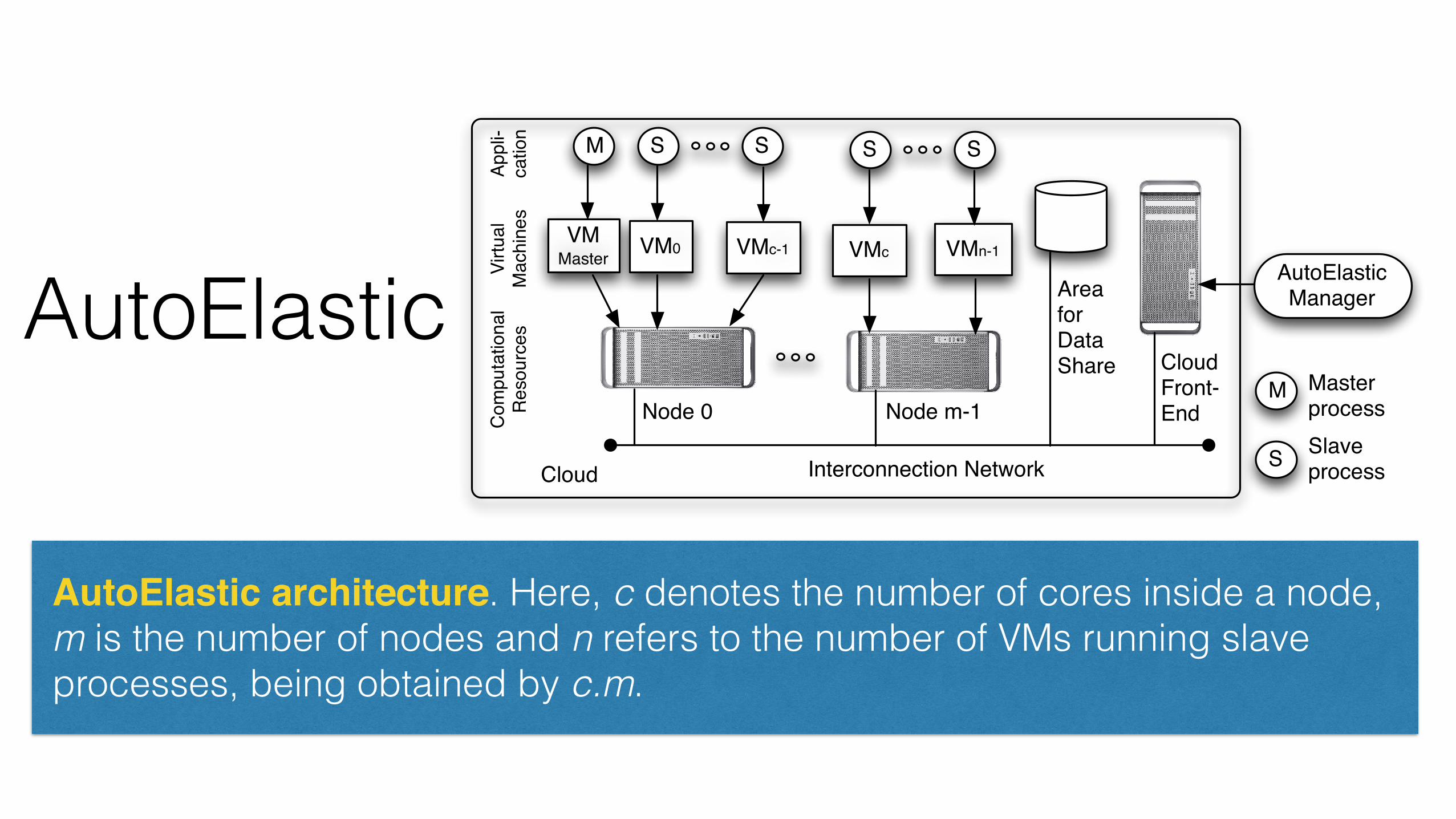
• Analyzing Asynchronous Elasticity: the goal isto present the benefits of asynchronous elasticityand the master process behavior when resourcereconfiguration takes place. Regarding the mea-sured metrics, we are observing both the times tolaunch a VM and to deliver it to application.
4.3.1 Performance and Elasticity Viability
Table 4 presents the results when executing the nu-merical integration application over the aforemen-tioned scenarios. The initial configuration starts from2 or 4 nodes, with each node having two processors.Therefore, 4 and 8 VMs are launched using 2 and 4nodes, respectively. As explained in Section 4.2, each(de)allocation involves 2 VMs because the nodes havetwo processors.
TABLE 4Elasticity results in two scenarios. Here, A, D and W
mean the Ascending, Descending and Wave loadpatterns. The times are expressed in seconds.
Star
ting
VM
sLo
ad
Scenario i: AutoElasticwith elasticity support
Scenario ii: AutoElasticwithout elasticity support
Time
Obser-vations Resource Cost Time Obser-
vations Resource Cost
4A 1978 65 26*4+27*6+12*8
= 362 716036 2426 81 81*4 =324 786024
D 1775 56 4*4+16*6+36*8 =400 710000 2397 81 81*4 =
324 776628
W 1895 59 4*4+22*6+33*8 =412 780740 2444 82 82*4 =
328 801632
8A 1789 57 39*6+18*8 = 378 676242 1555 52 52*8 =
416 646880
D 1570 52 8*6+44*8 = 400 628000 1561 52 52*8 =416 649376
W 1686 55 19*6+36*8 = 402 677772 1599 53 53*8 =424 677976
The results with the Constant load function werethe same in both scenarios because AutoElastic doesnot suggest any allocation or deallocation during theapplication execution. Consequently, 2360 s and 1467s were achieved when testing 4 and 8 VMs for theinitial situation. Specifically, as presented in Table 4,the use of 4 VMs at the program launch implies betterresults when comparing scenarios i and ii. Figure 9 (a)shows two moments of VM allocation when workingwith the Ascending function, providing a gain of19% in the application time. The Descending loadfunction achieves better results than the Ascending
IEEE TRANSACTIONS ON CLOUD COMPUTING, VOL X, NO Y, JANUARY 2015 10
of subintervals s between the limits a and b, which inthis experiment are 1 and 10, respectively. The largerthe number of intervals is, the greater the computa-tional load for generating the numerical integrationof the function. For the sake of simplicity, the samefunction is employed in the tests, but the number ofsubintervals for the integration varies.
Considering the cloud infrastructure, OpenNebulais executed in a cluster with 10 nodes. Each nodehas two processors, which are exclusively dedicatedto the cloud middleware. AutoElastic Manager runsoutside the Cloud and uses the OpenNebula API tocontrol and launch VMs. Our SLA was set up for aminimum of 2 nodes (4 VMs) and a maximum of 10nodes (20 VMs). Finally, we adopt a window parameterthat is equal to 6 in the load prediction (LP) functionto ensure that the weight of each observation is largerthan 1% (see Subsection 3.3 for detail).
Fig. 8. Graphical vision of the load patterns.
4.3 Results and Discussion
We divided this subsection in two parts to debateelasticity behavior. Following, we present the goalsand the metrics of each part:
• Performance and Elasticity Viability: the objectiveconsists in presenting performance results whencombining starting configurations, load patternsand two scenarios: (i) use of AutoElastic, enablingits self-organizing feature for dealing with elas-ticity; (ii) use of AutoElastic, managing load sit-uations but without taking any elasticity action.The metrics measured in this evaluation are: (i)the time in seconds to execute the application; (ii)the number of load observations of the AutoE-lastic manager; (iii) a comparison index definedas Resource and; (iv) a Cost function. This last,presented in Equation 5, means an adaptationof the cost of a parallel computation [18] forelastic environments. Instead of using the numberof processors, here resource is evaluated empir-ically taking into account both the number ofobservations as Obs(i) and the quantity of VMsi employed in each observation (see Equation 6).The AutoElastic’s goal is to offer an elasticitymodel that is costly viable. In other words, aconfiguration solution may be classified as a badif it is capable to reduce the execution time by thehalf with elasticity, but spends four times more
energy, increasing the costs for that. Therefore,considering the values of the cost function inTable 4, the objective is to preserve the truth ofInequality 7.
Cost = App T ime . Resource (5)such that
Resource =nX
i=1
(i⇥Obs(i)) (6)
then, the goal is to obtainCost
↵
Cost�
(7)
where ↵ and � refer to the AutoElastic executionwith and without elasticity support, respectively.
• Analyzing Asynchronous Elasticity: the goal isto present the benefits of asynchronous elasticityand the master process behavior when resourcereconfiguration takes place. Regarding the mea-sured metrics, we are observing both the times tolaunch a VM and to deliver it to application.
4.3.1 Performance and Elasticity Viability
Table 4 presents the results when executing the nu-merical integration application over the aforemen-tioned scenarios. The initial configuration starts from2 or 4 nodes, with each node having two processors.Therefore, 4 and 8 VMs are launched using 2 and 4nodes, respectively. As explained in Section 4.2, each(de)allocation involves 2 VMs because the nodes havetwo processors.
TABLE 4Elasticity results in two scenarios. Here, A, D and W
mean the Ascending, Descending and Wave loadpatterns. The times are expressed in seconds.
Star
ting
VM
sLo
ad
Scenario i: AutoElasticwith elasticity support
Scenario ii: AutoElasticwithout elasticity support
Time
Obser-vations Resource Cost Time Obser-
vations Resource Cost
4A 1978 65 26*4+27*6+12*8
= 362 716036 2426 81 81*4 =324 786024
D 1775 56 4*4+16*6+36*8 =400 710000 2397 81 81*4 =
324 776628
W 1895 59 4*4+22*6+33*8 =412 780740 2444 82 82*4 =
328 801632
8A 1789 57 39*6+18*8 = 378 676242 1555 52 52*8 =
416 646880
D 1570 52 8*6+44*8 = 400 628000 1561 52 52*8 =416 649376
W 1686 55 19*6+36*8 = 402 677772 1599 53 53*8 =424 677976
The results with the Constant load function werethe same in both scenarios because AutoElastic doesnot suggest any allocation or deallocation during theapplication execution. Consequently, 2360 s and 1467s were achieved when testing 4 and 8 VMs for theinitial situation. Specifically, as presented in Table 4,the use of 4 VMs at the program launch implies betterresults when comparing scenarios i and ii. Figure 9 (a)shows two moments of VM allocation when workingwith the Ascending function, providing a gain of19% in the application time. The Descending loadfunction achieves better results than the Ascending
Evaluation Methodology

Results
IEEE TRANSACTIONS ON CLOUD COMPUTING, VOL X, NO Y, JANUARY 2015 10
of subintervals s between the limits a and b, which inthis experiment are 1 and 10, respectively. The largerthe number of intervals is, the greater the computa-tional load for generating the numerical integrationof the function. For the sake of simplicity, the samefunction is employed in the tests, but the number ofsubintervals for the integration varies.
Considering the cloud infrastructure, OpenNebulais executed in a cluster with 10 nodes. Each nodehas two processors, which are exclusively dedicatedto the cloud middleware. AutoElastic Manager runsoutside the Cloud and uses the OpenNebula API tocontrol and launch VMs. Our SLA was set up for aminimum of 2 nodes (4 VMs) and a maximum of 10nodes (20 VMs). Finally, we adopt a window parameterthat is equal to 6 in the load prediction (LP) functionto ensure that the weight of each observation is largerthan 1% (see Subsection 3.3 for detail).
Fig. 8. Graphical vision of the load patterns.
4.3 Results and Discussion
We divided this subsection in two parts to debateelasticity behavior. Following, we present the goalsand the metrics of each part:
• Performance and Elasticity Viability: the objectiveconsists in presenting performance results whencombining starting configurations, load patternsand two scenarios: (i) use of AutoElastic, enablingits self-organizing feature for dealing with elas-ticity; (ii) use of AutoElastic, managing load sit-uations but without taking any elasticity action.The metrics measured in this evaluation are: (i)the time in seconds to execute the application; (ii)the number of load observations of the AutoE-lastic manager; (iii) a comparison index definedas Resource and; (iv) a Cost function. This last,presented in Equation 5, means an adaptationof the cost of a parallel computation [18] forelastic environments. Instead of using the numberof processors, here resource is evaluated empir-ically taking into account both the number ofobservations as Obs(i) and the quantity of VMsi employed in each observation (see Equation 6).The AutoElastic’s goal is to offer an elasticitymodel that is costly viable. In other words, aconfiguration solution may be classified as a badif it is capable to reduce the execution time by thehalf with elasticity, but spends four times more
energy, increasing the costs for that. Therefore,considering the values of the cost function inTable 4, the objective is to preserve the truth ofInequality 7.
Cost = App T ime . Resource (5)such that
Resource =nX
i=1
(i⇥Obs(i)) (6)
then, the goal is to obtainCost
↵
Cost�
(7)
where ↵ and � refer to the AutoElastic executionwith and without elasticity support, respectively.
• Analyzing Asynchronous Elasticity: the goal isto present the benefits of asynchronous elasticityand the master process behavior when resourcereconfiguration takes place. Regarding the mea-sured metrics, we are observing both the times tolaunch a VM and to deliver it to application.
4.3.1 Performance and Elasticity Viability
Table 4 presents the results when executing the nu-merical integration application over the aforemen-tioned scenarios. The initial configuration starts from2 or 4 nodes, with each node having two processors.Therefore, 4 and 8 VMs are launched using 2 and 4nodes, respectively. As explained in Section 4.2, each(de)allocation involves 2 VMs because the nodes havetwo processors.
TABLE 4Elasticity results in two scenarios. Here, A, D and W
mean the Ascending, Descending and Wave loadpatterns. The times are expressed in seconds.
Star
ting
VM
sLo
adScenario i: AutoElasticwith elasticity support
Scenario ii: AutoElasticwithout elasticity support
Time
Obser-vations Resource Cost Time Obser-
vations Resource Cost
4A 1978 65 26*4+27*6+12*8
= 362 716036 2426 81 81*4 =324 786024
D 1775 56 4*4+16*6+36*8 =400 710000 2397 81 81*4 =
324 776628
W 1895 59 4*4+22*6+33*8 =412 780740 2444 82 82*4 =
328 801632
8A 1789 57 39*6+18*8 = 378 676242 1555 52 52*8 =
416 646880
D 1570 52 8*6+44*8 = 400 628000 1561 52 52*8 =416 649376
W 1686 55 19*6+36*8 = 402 677772 1599 53 53*8 =424 677976
The results with the Constant load function werethe same in both scenarios because AutoElastic doesnot suggest any allocation or deallocation during theapplication execution. Consequently, 2360 s and 1467s were achieved when testing 4 and 8 VMs for theinitial situation. Specifically, as presented in Table 4,the use of 4 VMs at the program launch implies betterresults when comparing scenarios i and ii. Figure 9 (a)shows two moments of VM allocation when workingwith the Ascending function, providing a gain of19% in the application time. The Descending loadfunction achieves better results than the Ascending

ResultsIEEE TRANSACTIONS ON CLOUD COMPUTING, VOL X, NO Y, JANUARY 2015 12
IEEE TRANSACTIONS ON CLOUD COMPUTING, VOL X, NO Y, JANUARY 2016 12
0100200300400500600700800
012
024
136
148
160
272
286
599
011
1112
3113
5214
7216
1317
3818
6219
82
CPU
Loa
d
Time in Seconds(a)
0100200300400500600700800
0 90 203
295
388
500
594
688
778
869
959
1050
1141
1231
1325
1416
1507
1597
1731
CPU
Loa
d
Time in Seconds(b)
0100200300400500600700800
0 91 205
297
390
504
597
691
781
872
997
1088
1179
1293
1386
1480
1571
1662
1752
1864
CPU
Loa
d
Time in Seconds(c)
Fig. 8. CPU load behavior when using the following starting configuration: 2 nodes, 4 VMs and 4 CPUs
Fig. 9. CPU load behavior when using the following starting configuration: 4 nodes, 8 VMs and 8 CPUs
[2] Leander Beernaert, Miguel Matos, Ricardo Vilaca, and RuiOliveira. Automatic elasticity in openstack. In Proceedingsof the Workshop on Secure and Dependable Middleware for CloudMonitoring and Management, SDMCMM ’12, pages 2:1–2:6,New York, NY, USA, 2012. ACM.
[3] Roy Bryant, Alexey Tumanov, Olga Irzak, Adin Scannell,Kaustubh Joshi, Matti Hiltunen, Andres Lagar-Cavilla, andEyal de Lara. Kaleidoscope: cloud micro-elasticity via vmstate coloring. In Proceedings of the sixth conference on Computersystems, EuroSys ’11, pages 273–286, New York, NY, USA, 2011.ACM.
[4] Bin Cai, Feng Xu, Feng Ye, and Wenhuan Zhou. Researchand application of migrating legacy systems to the privatecloud platform with cloudstack. In Automation and Logistics(ICAL), 2012 IEEE International Conference on, pages 400 –404,aug. 2012.
[5] D. Chiu and G. Agrawal. Evaluating caching and storageoptions on the amazon web services cloud. In Grid Computing(GRID), 2010 11th IEEE/ACM International Conference on, pages17 –24, oct. 2010.
[6] Mihai Comanescu. Implementation of time-varying observersused in direct field orientation of motor drives by trapezoidal
integration. In Power Electronics, Machines and Drives (PEMD2012), 6th IET International Conference on, pages 1–6, 2012.
[7] Rostand Costa, Francisco Brasileiro, Guido L. de Souza Filho,and Denio M. Sousa. Just in Time Clouds: Enabling Highly-Elastic Public Clouds over Low Scale Amortized Resources.Technical report, Universidade Federal de Campina Grande,2010.
[8] Wesam Dawoud, Ibrahim Takouna, and Christoph Meinel.Elastic vm for cloud resources provisioning optimization. InAjith Abraham, Jaime Lloret Mauri, JohnF. Buford, JunichiSuzuki, and SabuM. Thampi, editors, Advances in Computingand Communications, volume 190 of Communications in Com-puter and Information Science, pages 431–445. Springer BerlinHeidelberg, 2011.
[9] Jennie Duggan and Michael Stonebraker. Incremental elasticityfor array databases. In Proceedings of the 2014 ACM SIGMODInternational Conference on Management of Data, SIGMOD ’14,pages 409–420, New York, NY, USA, 2014. ACM.
[10] Lixin Fu and C. Gondi. Cloud computing hosting. In ComputerScience and Information Technology (ICCSIT), 2010 3rd IEEEInternational Conference on, volume 3, pages 194–198, 2010.
[11] T. Fujii and M. Kimura. Analysis results on productivity
IEEE TRANSACTIONS ON CLOUD COMPUTING, VOL X, NO Y, JANUARY 2016 12
0100200300400500600700800
015
130
245
260
375
490
510
5612
0713
5815
0916
6018
1219
6321
1422
6524
16
CPU
Loa
d
Time in Seconds
AutoElastic without Elasticity Support, starting with 2 nodes and 4 VMs
0100200300400500600700800
012
024
036
148
260
372
384
496
410
8512
0613
2714
4715
6816
8818
0819
3020
5121
7222
93
CPU
Loa
d
Time in Seconds
AutoElastic without Elasticity Support, starting with 2 nodes and 4 VMs
0100200300400500600700800
015
030
245
260
375
490
610
5612
0813
5915
0916
5918
1019
6121
1322
6324
15
CPU
Loa
d
Time in Seconds
AutoElastic without Elasticity Support, starting with 2 nodes and 4 VMs
Fig. 8. CPU load behavior when using the following starting configuration: 2 nodes, 4 VMs and 4 CPUs
Fig. 9. CPU load behavior when using the following starting configuration: 4 nodes, 8 VMs and 8 CPUs
[2] Leander Beernaert, Miguel Matos, Ricardo Vilaca, and RuiOliveira. Automatic elasticity in openstack. In Proceedingsof the Workshop on Secure and Dependable Middleware for CloudMonitoring and Management, SDMCMM ’12, pages 2:1–2:6,New York, NY, USA, 2012. ACM.
[3] Roy Bryant, Alexey Tumanov, Olga Irzak, Adin Scannell,Kaustubh Joshi, Matti Hiltunen, Andres Lagar-Cavilla, andEyal de Lara. Kaleidoscope: cloud micro-elasticity via vmstate coloring. In Proceedings of the sixth conference on Computersystems, EuroSys ’11, pages 273–286, New York, NY, USA, 2011.ACM.
[4] Bin Cai, Feng Xu, Feng Ye, and Wenhuan Zhou. Researchand application of migrating legacy systems to the privatecloud platform with cloudstack. In Automation and Logistics(ICAL), 2012 IEEE International Conference on, pages 400 –404,aug. 2012.
[5] D. Chiu and G. Agrawal. Evaluating caching and storageoptions on the amazon web services cloud. In Grid Computing(GRID), 2010 11th IEEE/ACM International Conference on, pages17 –24, oct. 2010.
[6] Mihai Comanescu. Implementation of time-varying observersused in direct field orientation of motor drives by trapezoidal
integration. In Power Electronics, Machines and Drives (PEMD2012), 6th IET International Conference on, pages 1–6, 2012.
[7] Rostand Costa, Francisco Brasileiro, Guido L. de Souza Filho,and Denio M. Sousa. Just in Time Clouds: Enabling Highly-Elastic Public Clouds over Low Scale Amortized Resources.Technical report, Universidade Federal de Campina Grande,2010.
[8] Wesam Dawoud, Ibrahim Takouna, and Christoph Meinel.Elastic vm for cloud resources provisioning optimization. InAjith Abraham, Jaime Lloret Mauri, JohnF. Buford, JunichiSuzuki, and SabuM. Thampi, editors, Advances in Computingand Communications, volume 190 of Communications in Com-puter and Information Science, pages 431–445. Springer BerlinHeidelberg, 2011.
[9] Jennie Duggan and Michael Stonebraker. Incremental elasticityfor array databases. In Proceedings of the 2014 ACM SIGMODInternational Conference on Management of Data, SIGMOD ’14,pages 409–420, New York, NY, USA, 2014. ACM.
[10] Lixin Fu and C. Gondi. Cloud computing hosting. In ComputerScience and Information Technology (ICCSIT), 2010 3rd IEEEInternational Conference on, volume 3, pages 194–198, 2010.
[11] T. Fujii and M. Kimura. Analysis results on productivity
(a) (b) (c)
IEEE TRANSACTIONS ON CLOUD COMPUTING, VOL X, NO Y, JANUARY 2016 12
Allocated Used Maximum Threshold Minimum Threshold
Fig. 8. CPU load behavior when using the following starting configuration: 2 nodes, 4 VMs and 4 CPUs
Fig. 9. CPU load behavior when using the following starting configuration: 4 nodes, 8 VMs and 8 CPUs
[2] Leander Beernaert, Miguel Matos, Ricardo Vilaca, and RuiOliveira. Automatic elasticity in openstack. In Proceedingsof the Workshop on Secure and Dependable Middleware for CloudMonitoring and Management, SDMCMM ’12, pages 2:1–2:6,New York, NY, USA, 2012. ACM.
[3] Roy Bryant, Alexey Tumanov, Olga Irzak, Adin Scannell,Kaustubh Joshi, Matti Hiltunen, Andres Lagar-Cavilla, andEyal de Lara. Kaleidoscope: cloud micro-elasticity via vmstate coloring. In Proceedings of the sixth conference on Computersystems, EuroSys ’11, pages 273–286, New York, NY, USA, 2011.ACM.
[4] Bin Cai, Feng Xu, Feng Ye, and Wenhuan Zhou. Researchand application of migrating legacy systems to the privatecloud platform with cloudstack. In Automation and Logistics(ICAL), 2012 IEEE International Conference on, pages 400 –404,aug. 2012.
[5] D. Chiu and G. Agrawal. Evaluating caching and storageoptions on the amazon web services cloud. In Grid Computing(GRID), 2010 11th IEEE/ACM International Conference on, pages17 –24, oct. 2010.
[6] Mihai Comanescu. Implementation of time-varying observersused in direct field orientation of motor drives by trapezoidal
integration. In Power Electronics, Machines and Drives (PEMD2012), 6th IET International Conference on, pages 1–6, 2012.
[7] Rostand Costa, Francisco Brasileiro, Guido L. de Souza Filho,and Denio M. Sousa. Just in Time Clouds: Enabling Highly-Elastic Public Clouds over Low Scale Amortized Resources.Technical report, Universidade Federal de Campina Grande,2010.
[8] Wesam Dawoud, Ibrahim Takouna, and Christoph Meinel.Elastic vm for cloud resources provisioning optimization. InAjith Abraham, Jaime Lloret Mauri, JohnF. Buford, JunichiSuzuki, and SabuM. Thampi, editors, Advances in Computingand Communications, volume 190 of Communications in Com-puter and Information Science, pages 431–445. Springer BerlinHeidelberg, 2011.
[9] Jennie Duggan and Michael Stonebraker. Incremental elasticityfor array databases. In Proceedings of the 2014 ACM SIGMODInternational Conference on Management of Data, SIGMOD ’14,pages 409–420, New York, NY, USA, 2014. ACM.
[10] Lixin Fu and C. Gondi. Cloud computing hosting. In ComputerScience and Information Technology (ICCSIT), 2010 3rd IEEEInternational Conference on, volume 3, pages 194–198, 2010.
[11] T. Fujii and M. Kimura. Analysis results on productivity
Fig. 9. CPU behavior when starting with 2 nodes and the following load patterns: (a) Ascending; (b) Descending;(c) Wave. Non-elastic and elastic executions are expressed in the upper and the bottom parts, respectively.
IEEE TRANSACTIONS ON CLOUD COMPUTING, VOL X, NO Y, JANUARY 2016 12
Fig. 8. CPU load behavior when using the following starting configuration: 2 nodes, 4 VMs and 4 CPUs
Fig. 9. CPU load behavior when using the following starting configuration: 4 nodes, 8 VMs and 8 CPUs
[2] Leander Beernaert, Miguel Matos, Ricardo Vilaca, and RuiOliveira. Automatic elasticity in openstack. In Proceedingsof the Workshop on Secure and Dependable Middleware for CloudMonitoring and Management, SDMCMM ’12, pages 2:1–2:6,New York, NY, USA, 2012. ACM.
[3] Roy Bryant, Alexey Tumanov, Olga Irzak, Adin Scannell,Kaustubh Joshi, Matti Hiltunen, Andres Lagar-Cavilla, andEyal de Lara. Kaleidoscope: cloud micro-elasticity via vmstate coloring. In Proceedings of the sixth conference on Computersystems, EuroSys ’11, pages 273–286, New York, NY, USA, 2011.ACM.
[4] Bin Cai, Feng Xu, Feng Ye, and Wenhuan Zhou. Researchand application of migrating legacy systems to the privatecloud platform with cloudstack. In Automation and Logistics(ICAL), 2012 IEEE International Conference on, pages 400 –404,aug. 2012.
[5] D. Chiu and G. Agrawal. Evaluating caching and storageoptions on the amazon web services cloud. In Grid Computing(GRID), 2010 11th IEEE/ACM International Conference on, pages17 –24, oct. 2010.
[6] Mihai Comanescu. Implementation of time-varying observersused in direct field orientation of motor drives by trapezoidal
integration. In Power Electronics, Machines and Drives (PEMD2012), 6th IET International Conference on, pages 1–6, 2012.
[7] Rostand Costa, Francisco Brasileiro, Guido L. de Souza Filho,and Denio M. Sousa. Just in Time Clouds: Enabling Highly-Elastic Public Clouds over Low Scale Amortized Resources.Technical report, Universidade Federal de Campina Grande,2010.
[8] Wesam Dawoud, Ibrahim Takouna, and Christoph Meinel.Elastic vm for cloud resources provisioning optimization. InAjith Abraham, Jaime Lloret Mauri, JohnF. Buford, JunichiSuzuki, and SabuM. Thampi, editors, Advances in Computingand Communications, volume 190 of Communications in Com-puter and Information Science, pages 431–445. Springer BerlinHeidelberg, 2011.
[9] Jennie Duggan and Michael Stonebraker. Incremental elasticityfor array databases. In Proceedings of the 2014 ACM SIGMODInternational Conference on Management of Data, SIGMOD ’14,pages 409–420, New York, NY, USA, 2014. ACM.
[10] Lixin Fu and C. Gondi. Cloud computing hosting. In ComputerScience and Information Technology (ICCSIT), 2010 3rd IEEEInternational Conference on, volume 3, pages 194–198, 2010.
[11] T. Fujii and M. Kimura. Analysis results on productivity
(a) (b) (c)
Fig. 10. CPU behavior when starting with 4 nodes and the following load patterns: (a) Ascending; (b)Descending; (c) Wave. Non-elastic execution is in the upper part, while elasticity capacity appears in the bottom.
action, the master must establish two new connectionssynchronously. Only after completing this task, themaster obtains the roll of current processes and canpass a uniform part of the work for each process.Moreover, it is possible to observe a short reductionin the CPU usage after crossing 1770 s because ofthe workload spread among more processes after anallocation action.
5 CONCLUSION
Cloud elasticity has been used for scaling traditionalweb applications to handle unpredictable workloads,which enables companies to avoid downfalls that areinvolved with fixed provisioning (over- and under-provisioning). Considering the current scenario, thisarticle addressed cloud elasticity for HPC applica-tions by presenting a model denoted AutoElastic. Inbrief, AutoElastic self-organizes the number of virtualmachines without any user intervention, providing
benefits for both the cloud administrator (better en-ergy consumption and resource sharing among theusers) and the cloud user (application performanceand overhead when migrating to the cloud). As themain scientific contribution to the state-of-the-art inthe confluence of cloud and HPC systems, AutoElasticproposes the use of asynchronism for elasticity man-agement. This feature implies not blocking the parallelapplication while a newly allocated VM is beingtransferred, which offers one of the most importantcapabilities of the cloud without prohibitive costs.
The AutoElastic’s model for applications matchesthe socket-programming style that is offered by MPI-2, in which new processes can be easily added or re-moved, connected and disconnected, from the parallelcomputation. The evaluation demonstrated encourag-ing results on using the CPU metric for HPC elasticity.Despite addressing a processing-intensive application,they revealed that the load does not always remainclose to 100%. We measured that the overhead to
Results
IEEE TRANSACTIONS ON CLOUD COMPUTING, VOL X, NO Y, JANUARY 2015 13
CPU
load
%
0
20
40
60
80
100CPU 1
CPU 2
Time in seconds
700690 710 720
CPU
load
%
20
40
60
80
100
Time in seconds1760 1770 1780 1790 1800
(a) Impact of VM deallocation in running VMs
(b) Impact of VM allocation in running VMs
Moment where the master closes the connection to
other 2 processes
Moment where the master establishes the connection with two newer processes
680
CPU 1
CPU 2
Fig. 11. Impact in the running processes regardingthe disconnection and connection of other processes ofthe parallel application: (a) start with 4 VMs and Wavefunction; (b) start with 4 VMs and Ascending function
double the VMs is on average 3 m and 36 s, butduring this interval, the application continues to exe-cute normally. Furthermore, the evaluation presenteda decision function that is expressed by multiplyingthe resource consumption by the performance, whereAutoElastic achieved 5 positive results on 6 observa-tions when compared with a non-elastic execution.
In addition to the use of AutoElastic on privateclouds, the elasticity model can be adapted to run overAmazon AWS or Windows Azure. We also concernthe study of network and memory elasticity to employthese capabilities in the next versions of AutoElas-tic. Although the numerical integration application isuseful to evaluate AutoElastic, we intend to explorehighly irregular applications [17]. Last, we have plansto extend AutoElastic to cover divide-and-conquerand bulk-synchronous parallel applications.
REFERENCES[1] W. Lin, J. Z. Wang, C. Liang, and D. Qi, “A threshold-based
dynamic resource allocation scheme for cloud computing,”Procedia Engineering, vol. 23, no. 0, pp. 695 – 703, 2011.
[2] J. Duggan and M. Stonebraker, “Incremental elasticity forarray databases,” in Proceedings of the 2014 ACM SIGMODInternational Conference on Management of Data, New York, NY,USA: ACM, pp. 409–420, 2014.
[3] P. Jamshidi, A. Ahmad, and C. Pahl, “Autonomic resourceprovisioning for cloud-based software,” in Proc. of the 9th Int.Symp. on Software Engineering for Adaptive and Self-ManagingSystems, New York, NY, USA: ACM, pp. 95–104, 2014.
[4] W. Dawoud, I. Takouna, and C. Meinel, “Elastic vm for cloudresources provisioning optimization,” in Advances in Comput-ing and Communications, ser. Comm. in Comp. and InformationScience, Springer Berlin, vol. 190, pp. 431–445, 2011.
[5] S. Imai, T. Chestna, and C. A. Varela, “Elastic scalable cloudcomputing using application-level migration,” in Proc. of theInt. Conf. on Utility and Cloud Computing, Washington, DC,USA: IEEE Computer Society, pp. 91–98, 2012.
[6] M. Mao, J. Li, and M. Humphrey, “Cloud auto-scaling withdeadline and budget constraints,” in Grid Computing (GRID),11th IEEE/ACM Int. Conf. on, pp. 41 –48, 2010.
[7] R. Han, L. Guo, M. M. Ghanem, and Y. Guo, “Lightweightresource scaling for cloud applications,” Cluster Computing andthe Grid, IEEE Int. Symp. on, vol. 0, pp. 644–651, 2012.
[8] A. Raveendran, T. Bicer, and G. Agrawal, “A framework forelastic execution of existing mpi programs,” in Proc, of the Int.Symp. on Parallel and Dist. Processing Workshops and PhD Forum,Washington, DC, USA: IEEE Comp. Society, pp. 940–947, 2011.
[9] G. Galante and L. C. E. d. Bona, “A survey on cloud com-puting elasticity,” in Proc. of the Int. Conf. on Utility and CloudComputing, Washington: IEEE Comp. Soc., pp. 263–270, 2012.
[10] A. N. Toosi, R. N. Calheiros, and R. Buyya, “Interconnectedcloud computing environments: Challenges, taxonomy, andsurvey,” ACM Comput. Surv., vol. 47, no. 1, pp. 7:1–7:47, 2014.
[11] D. Chiu and G. Agrawal, “Evaluating caching and storageoptions on the amazon web services cloud,” in Grid Computing(GRID), 2010 11th IEEE/ACM Int. Conf. on, pp. 17 –24, 2010.
[12] E. Lusk, “MPI-2: standards beyond the message-passingmodel,” in Massively Parallel Programming Models, Proc.. ThirdWorking Conf. on, pp. 43–49, 1997
[13] D. Rajan, A. Canino, J. A. Izaguirre, and D. Thain, “Convertinga high performance application to an elastic cloud applica-tion,” in Proc. of the Conf. on Cloud Computing Technology andScience, Washington, USA: IEEE Comp. Soc., pp. 383–390, 2011.
[14] T. Knauth and C. Fetzer, “Scaling non-elastic applicationsusing virtual machines,” in Cloud Computing (CLOUD), IEEEInt. Conf. on, pp. 468 –475, 2011.
[15] K. Kumar, J. Feng, Y. Nimmagadda, and Y.-H. Lu, “Resourceallocation for real-time tasks using cloud computing,” in Com-puter Communications and Networks (ICCCN), Int. Conf. on, pp.1 –7, 2011.
[16] E. Michon, J. Gossa, and S. Genaud, “Free elasticity and freecpu power for scientific workloads on iaas clouds,” in Paralleland Distributed Systems (ICPADS), Int. Conf. on, pp. 85 –92, 2012.
[17] K. Jackson, L. Ramakrishnan, K. Muriki, S. Canon, S. Cho-lia, J. Shalf, H. J. Wasserman, and N. Wright, “Performanceanalysis of high performance computing applications on theamazon web services cloud,” in Cloud Computing Technologyand Science (CloudCom), Int. Conf. on, pp. 159–168, 2010.
[18] B. Wilkinson and C. Allen, Parallel Programming: Techniquesand Applications Using Networked Workstations and ParallelComputers, Pearson/Prentice Hall, 2005.
[19] A. Tanenbaum, Computer Networks, 4th ed. Upper SaddleRiver, New Jersey: Prentice Hall PTR, 2003.
[20] D. Milojicic, I. M. Llorente, and R. S. Montero, “Opennebula:A cloud management tool,” Internet Computing, IEEE, vol. 15,no. 2, pp. 11 –14, march-april 2011.
[21] U. Sharma, P. Shenoy, S. Sahu, and A. Shaikh, “A cost-awareelasticity provisioning system for the cloud,” in Proc. of the2011 Int. Conf. on Distributed Computing Systems, Washington,DC, USA: IEEE Computer Society, pp. 559–570, 2011.
[22] A. Lonea, D. Popescu, and O. Prostean, “A survey of manage-ment interfaces for eucalyptus cloud,” in Applied Comp. Intellig.and Informatics (SACI), IEEE Symp., pp. 261–266, 2012.
[23] E. Roloff, F. Birck, M. Diener, A. Carissimi, and P. Navaux,“Evaluating high performance computing on the windowsazure platform,” in Cloud Computing (CLOUD), 2012 IEEE 5thInt. Conf. on, pp. 803 –810, 2012.
[24] P. Marshall, K. Keahey, and T. Freeman, “Elastic site: Usingclouds to elastically extend site resources,” in Proc. of theIEEE/ACM Int. Conf. on Cluster, Cloud and Grid Computing,Washington, DC, USA: IEEE Comp. Society, pp. 43–52, 2010.
[25] X. Wen, G. Gu, Q. Li, Y. Gao, and X. Zhang, “Compari-son of open-source cloud management platforms: Openstackand opennebula,” in Fuzzy Systems and Knowledge Discovery(FSKD), 2012 9th Int. Conf. on, pp. 2457 –2461, 2012.
[26] B. Cai, F. Xu, F. Ye, and W. Zhou, “Research and application ofmigrating legacy systems to the private cloud platform withcloudstack,” in Automation and Logistics (ICAL), IEEE Int. Conf.on, pp. 400 –404, 2012.

Conclusion
Main ideasAsynchronous Elasticity
Weighted Moving Average = Aging concept
Limitations
Reactive Elasticity
Thresholds are fixed
Elasticity actions take place after observing modifications in the
application’s demand. VM launching is time consuming.
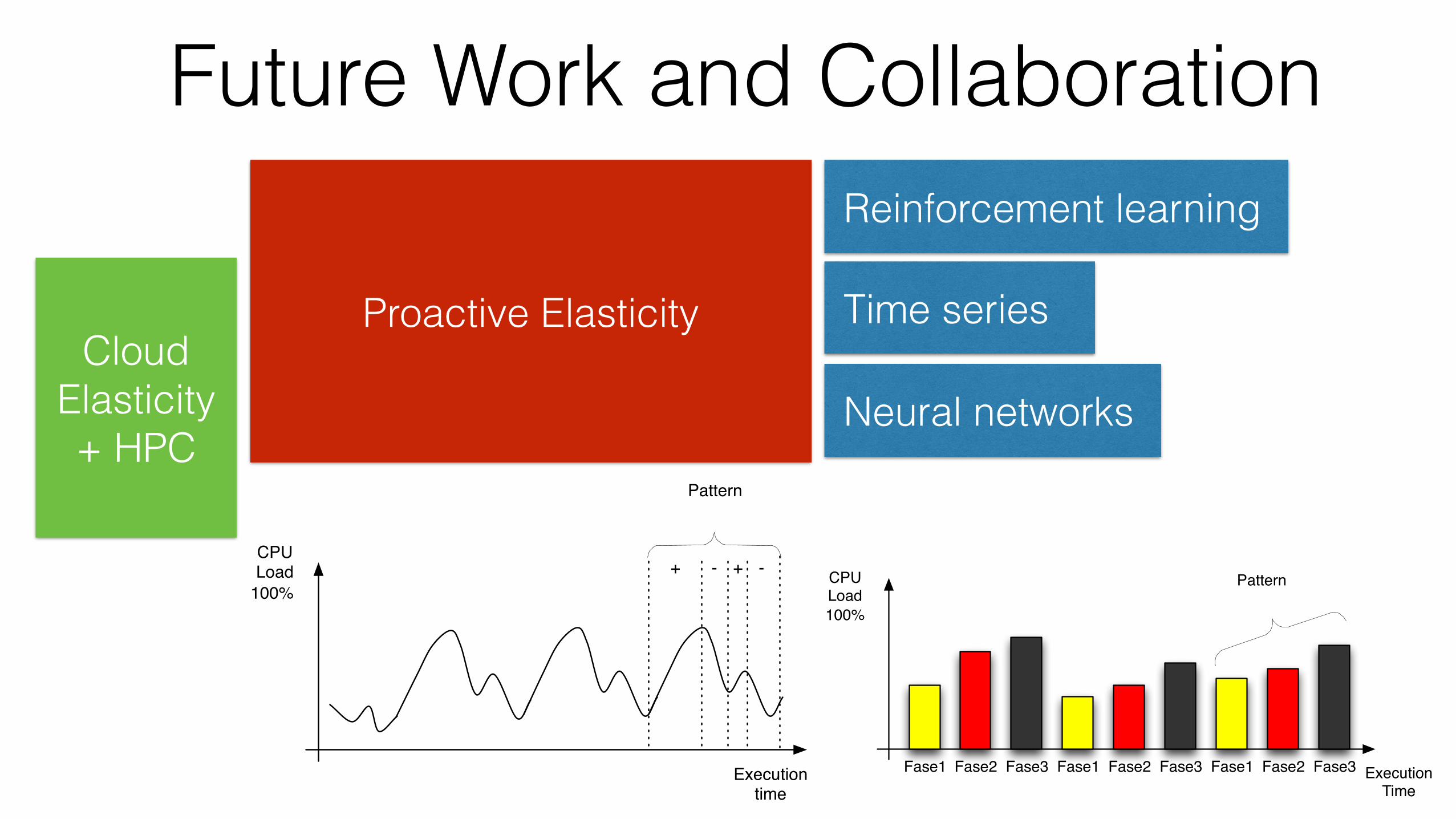
Future Work and Collaboration
Proactive Elasticity
Reinforcement learning
Time series
Neural networksCloud
Elasticity + HPC
CPULoad
Executiontime
100%
Pattern
+ - -+ CPULoad
ExecutionTime
100%
Fase1 Fase2 Fase3 Fase1 Fase2 Fase3 Fase1 Fase2 Fase3
Pattern

Future Work and CollaborationAdaptable thresholds
Covering Divide-and-Conquer and Bulk-Synchronous Parallel
applications
Cloud Elasticity +
HPC

Future Work and Collaboration
Internet of Things -
Scalability
Internet of ThingsMiddleware
Collection and Aggregation of Data
Processed Data about IoT devices
IoT-Enabled DevicesUser Applications
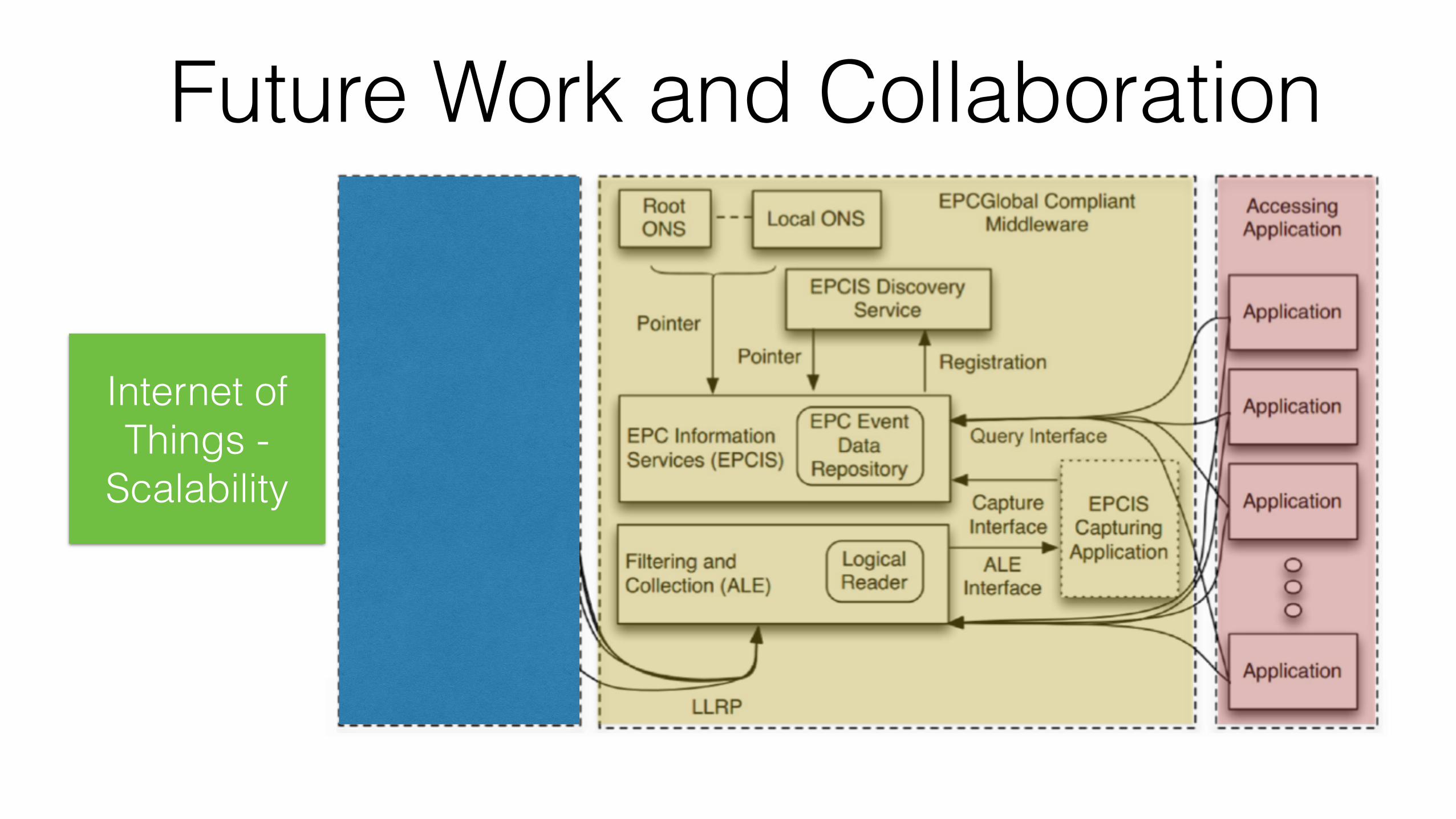
Future Work and Collaboration
Internet of Things -
Scalability
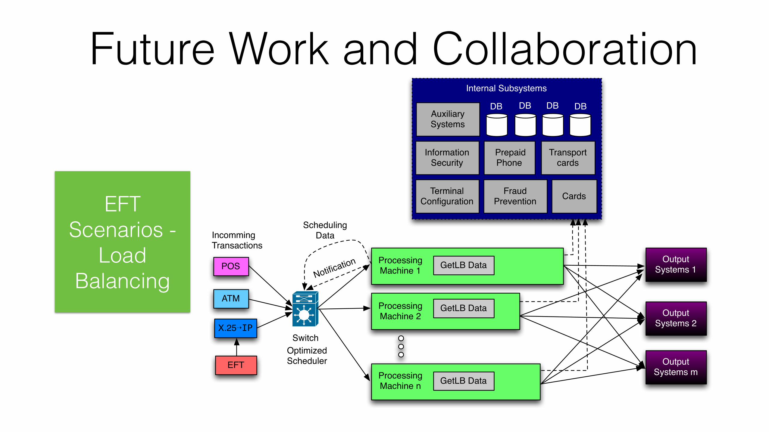
Future Work and Collaboration
EFT Scenarios -
Load Balancing
Cards
Prepaid Phone
Transport cards
Terminal Configuration
Information Security
Fraud Prevention
ProcessingMachine 1
Internal Subsystems
POS
ATM
X.25➝IP
Output Systems 1
Output Systems 2
Output Systems m
Incomming Transactions
Switch
DB DB DB DBAuxiliary Systems
EFT
ProcessingMachine 2
ProcessingMachine n
Optimized Scheduler
GetLB Data
GetLB Data
GetLB Data
SchedulingData
Notification