Automatic Loudspeaker

Location Detection

for use in

Ambisonic Systems

Robert A. Humphrey

4th Year Project Report for the degree of MEng

in Electronic Engineering

June 2006

STINT contract number: IG2002-2049

Abstract

To allow easier configuration of Ambisonic surround sound systems different meth-

ods of automatically locating loudspeakers have been considered: first, separation

measurements using a single microphone and propagation delays; second, angle

measurement using a SoundField microphone and amplitude differences; and third,

angle measurement using multiple microphones and propagation delays. Tests

on the first two were conducted, and accuracies to less than a sample-interval

for propagation delays and to within ±1◦ for angle measurements are shown to

be feasible. A utility to allow continuous multi-channel audio input and output

within MATLAB has been designed and using this an Ambisonics decoder has

been implemented.

Acknowledgements

The author would like to thank the following people for their help and support

throughout the course of the project:

� Everyone at the Department of Speech, Music and Hearing (TMH) at the

Royal Institute of Technology (KTH), Stockholm, for making the time there

productive and enjoyable, and specifically Svante Granqvist, Sten Ternstrom

and Mikael Bohman.

� Damian Murphy, Jez Wells and Myles Capstick for their valued input.

� Catherine Humphrey, Cally Nixon, Lorna Mitchell and Tim Clarke for pro-

viding many hours of proof reading.

� Vıctor Luana at the Quantum Chemistry Group, Departamento de Quımica

Fısica y Analıtica, Universidad de Oviedo, Spain, for generating the images

shown in figure 2.1.

i

Contents

Glossary of Terms vii

1 Introduction 1

2 Background 3

2.1 Surround sound history . . . . . . . . . . . . . . . . . . . . . . . . . 3

2.2 Ambisonics . . . . . . . . . . . . . . . . . . . . . . . . . . . . . . . 5

3 Project Aims 9

3.1 Loudspeaker Layout Characterisation . . . . . . . . . . . . . . . . . 10

3.2 Decoding a B-Format signal . . . . . . . . . . . . . . . . . . . . . . 12

3.3 Practical Implementation . . . . . . . . . . . . . . . . . . . . . . . . 13

3.4 Summary . . . . . . . . . . . . . . . . . . . . . . . . . . . . . . . . 14

4 Test Environment 15

4.1 Audio within MATLAB . . . . . . . . . . . . . . . . . . . . . . . . 16

4.2 Alternatives to MATLAB on Windows . . . . . . . . . . . . . . . . 21

ii

4.3 Using PortAudio within MATLAB . . . . . . . . . . . . . . . . . . 24

5 Audio Handling Utility Requirements 26

6 Design of MEX-file Core 31

6.1 Providing multiple functions . . . . . . . . . . . . . . . . . . . . . . 31

6.2 Command Dispatching . . . . . . . . . . . . . . . . . . . . . . . . . 33

6.3 Implementation . . . . . . . . . . . . . . . . . . . . . . . . . . . . . 37

6.4 Testing . . . . . . . . . . . . . . . . . . . . . . . . . . . . . . . . . . 42

7 Design of playrec MEX-file 44

7.1 Request Pages . . . . . . . . . . . . . . . . . . . . . . . . . . . . . . 44

7.2 Thread safe design . . . . . . . . . . . . . . . . . . . . . . . . . . . 46

7.3 Page Structures . . . . . . . . . . . . . . . . . . . . . . . . . . . . . 53

7.4 Implementation . . . . . . . . . . . . . . . . . . . . . . . . . . . . . 57

7.5 Testing . . . . . . . . . . . . . . . . . . . . . . . . . . . . . . . . . . 58

8 Excitation Signals 65

8.1 Signal Types . . . . . . . . . . . . . . . . . . . . . . . . . . . . . . . 66

8.2 Signal Creation and Processing . . . . . . . . . . . . . . . . . . . . 71

8.3 Test Implementation . . . . . . . . . . . . . . . . . . . . . . . . . . 77

8.4 Accuracy and Repeatability . . . . . . . . . . . . . . . . . . . . . . 80

iii

9 Delay Measurements 82

9.1 Influencing Factors . . . . . . . . . . . . . . . . . . . . . . . . . . . 82

9.2 Test Setup . . . . . . . . . . . . . . . . . . . . . . . . . . . . . . . . 84

9.3 Loop Back Analysis . . . . . . . . . . . . . . . . . . . . . . . . . . . 87

9.4 Microphone Signal Analysis . . . . . . . . . . . . . . . . . . . . . . 93

10 SoundField Microphone Measurements 103

10.1 Angle Measurement Theory . . . . . . . . . . . . . . . . . . . . . . 103

10.2 Test Setup . . . . . . . . . . . . . . . . . . . . . . . . . . . . . . . . 105

10.3 Analysis . . . . . . . . . . . . . . . . . . . . . . . . . . . . . . . . . 109

11 Multiple Microphone Measurements 119

11.1 Theory . . . . . . . . . . . . . . . . . . . . . . . . . . . . . . . . . . 119

11.2 Planned Testing . . . . . . . . . . . . . . . . . . . . . . . . . . . . . 121

12 Ambisonics Decoding 123

12.1 Decoder Types . . . . . . . . . . . . . . . . . . . . . . . . . . . . . 124

12.2 Decoder Implementation . . . . . . . . . . . . . . . . . . . . . . . . 125

13 Overall System Design 128

13.1 Signal Decoding . . . . . . . . . . . . . . . . . . . . . . . . . . . . . 128

13.2 Loudspeaker Location Detection . . . . . . . . . . . . . . . . . . . . 130

13.3 Summary . . . . . . . . . . . . . . . . . . . . . . . . . . . . . . . . 131

iv

14 Project Management 133

15 Further Work 136

15.1 Audio Handling within MATLAB . . . . . . . . . . . . . . . . . . . 136

15.2 Loudspeaker Location Detection . . . . . . . . . . . . . . . . . . . . 137

15.3 Ambisonics Decoding . . . . . . . . . . . . . . . . . . . . . . . . . . 140

15.4 Complete System Implementation . . . . . . . . . . . . . . . . . . . 140

16 Conclusion 142

References 144

Appendices 150

A MEX-file Overview 150

A.1 Entry Point Function . . . . . . . . . . . . . . . . . . . . . . . . . . 150

A.2 Memory management . . . . . . . . . . . . . . . . . . . . . . . . . . 151

A.3 Textual Display . . . . . . . . . . . . . . . . . . . . . . . . . . . . . 152

A.4 Providing Help . . . . . . . . . . . . . . . . . . . . . . . . . . . . . 153

B PortAudio Overview 154

C Configuring Visual Studio 157

v

D playrec Utility Help Information 161

D.1 Utility overview . . . . . . . . . . . . . . . . . . . . . . . . . . . . . 161

D.2 Command specific help . . . . . . . . . . . . . . . . . . . . . . . . . 164

E Equipment List 180

F B-Format Signal Manipulation 182

F.1 Soundfield Rotation . . . . . . . . . . . . . . . . . . . . . . . . . . . 182

F.2 Virtual Microphones . . . . . . . . . . . . . . . . . . . . . . . . . . 184

G CD Contents 187

G.1 Documentation . . . . . . . . . . . . . . . . . . . . . . . . . . . . . 187

G.2 MATLAB code . . . . . . . . . . . . . . . . . . . . . . . . . . . . . 187

G.3 playrec utility . . . . . . . . . . . . . . . . . . . . . . . . . . . . . . 189

vi

Glossary of Terms

Abbreviation Details

A/D Analogue-to-Digital (converter)

ALSA Advanced Linux Sound Architecture

API Application Program Interface

ASIO Audio Stream Input/Output

D/A Digital-to-Analogue (converter)

FHT Fast Hadamard Transform

FIR Finite Impulse Response

GUI Graphical User Interface

IDE Integrated Development Environment

IDFT Inverse Discrete Fourier Transform

IR Impulse Response

IRS Inverse Repeated Sequence

MLS Maximum Length Sequence

MME (Windows) Multimedia Extension

OATSP Optimum Aoshima’s Time-Stretched Pulse

PC Personal Computer

PD Pure Data

RF Radio Frequency

SDK Software Development Kit

SNR Signal-to-Noise Ratio

TSP Time-Stretched Pulse

VST Virtual Studio Technology

vii

Chapter 1

Introduction

With the ever increasing popularity of surround sound systems there is always the

question ‘what will be next?’. One possible answer, although not a new technol-

ogy, is Ambisonics1. This allows for much greater flexibility in the number and

arrangement of loudspeakers when compared to the more conventional 5.1 sur-

round sound systems. Additionally it provides better sound localisation behind

the listener and the ability to include ‘height’ information. However, to obtain the

best performance the loudspeaker positioning is much more critical than with other

systems. Although the standard loudspeaker arrangements are always regular, it

is also possible to use irregular arrangements provided the loudspeaker locations

are known by the signal decoder. Configuring this can be time consuming and

potentially inaccurate, requiring fine tuning to obtain the best performance which

is not appealing to those who are far more used to things working straight out the

box. This project investigated how to determine the location of loudspeakers in a

room automatically, thus enabling much easier system setup.

Chapter 2 provides background information relevant to this project, specifically

concentrating on Ambisonics and its differences from other surround sound sys-

tems. The aims for the project are then given in chapter 3, considering the com-

1Ambisonics is a registered trademark of Nimbus Communications International

1

plete automated system in three sections: determining the location of the loud-

speakers, implementing an Ambisonics decoder, and overall system implementa-

tion. In chapter 4 details of the tests used to determine the most suitable computer

configuration for the remainder of the project are given, resulting in the require-

ment to develop a multi-channel audio handling utility for MATLAB. An overview

of the significant parts of the development of this utility, from requirements to im-

plementation and testing, are provided in chapters 5 to 7.

In chapter 8, different excitation signals are considered that could be used to de-

termine the location of a loudspeaker, including implementation information for

the signals to be used in all subsequent tests. The first set of tests conducted

and their results are detailed in chapter 9. These tests used a single microphone

and were designed to determine the practical accuracy possible when measuring

distances using propagation delays. Chapter 10 then describes the test configu-

ration and results obtained when using a SoundField microphone to measure the

angle between loudspeakers. Methods using multiple microphones to determine

the location of a loudspeaker are given in chapter 11.

A basic continuous Ambisonics decoder implemented within MATLAB is described

in chapter 12 and then the possibility of implementing a complete, automati-

cally configuring, Ambisonics system using wireless communications is discussed

in chapter 13. An overview of the project time management is given in chap-

ter 14, potential further work to extend this project is outlined in chapter 15 with

chapter 16 bringing together conclusions on the project.

The project was conducted at the Department of Speech, Music and Hearing

(TMH), in the School of Computer Science and Communication at the Royal

Institute of Technology (KTH), Stockholm. Funding was supplied by both The

Swedish Foundation for International Cooperation in Research and Higher Edu-

cation (STINT) and the UK Socrates-Erasmus Council.

2

Chapter 2

Background

The technology used in the reproduction of sound is continuously advancing in

all areas, ranging from the initial recording through to signal processing, storage,

transmission and final output from loudspeakers. This section provides a brief

overview of some of these developments that are specifically relevant to this project.

2.1 Surround sound history

Sound reproduction devices have become commonplace in many homes in the

western world, appearing in different forms including computers, mobile phones,

televisions, MP3 players, stereos and surround sound systems. These can all,

however, be grouped into three categories: single (mono), double (stereo) and

multiple (surround) channel devices.

Mono recording and playback devices were first created over a century ago and

since then various advances have occurred. The most significant of these was the

development of the stereo system as we know it today by Alan Blumlein of EMI

and Harvey Fletcher of Bell Labs, amongst others, in the 1930s. Although this

work also considered the use of many more than 2 channels, it was only in the 1970s

3

that consumer multi-channel systems appeared[31]. These were quadraphonic (or

quad) systems using four loudspeakers placed evenly around the listener. This

technique was based on the simplified ‘intensity panning’, or ‘pan-pot’, approach

already being used for stereo systems: that is, altering the relative amplitude of a

signal sent to each loudspeaker to generate phantom images appearing somewhere

between them[21]. However, as summarised by Gerzon[15] and Malham[21], there

are many other mechanisms besides intensity difference used to provide cues to

the location of a sound source. Without taking more of these into account when

trying to create phantom images the results can be very poor[7, 21, 29]:

� instability and noticeable elevation[5] of images occurs in addition to a “hole

in the middle” effect if the front loudspeakers are separated by more than

60◦, as with quadraphonics;

� there is generally poor localisation of sound sources behind the listener;

� localisation is between poor and nonexistent to the sides of the listener;

� image localisation is sensitive to both misplacement of loudspeakers and head

position.

To avoid such problems the surround sound systems that were successful from

just after this era, which are still in use in a similar form today, do not attempt

to create a full 360◦ soundfield of stable phantom images. Instead, they tend to

use 3 front loudspeakers to generate stable front phantom images (especially for

off-centre listening), whilst additional loudspeakers around the listener produce a

diffuse ‘surround’ sound, such as in the common 5.1 surround sound systems[31].

An alternative approach to surround sound reproduction is to “attempt to recon-

struct in the listening space a set of audio waveforms which matches those in the

recording space”[22]. To fully achieve this a very large1 number of channels would

1Values quoted include 400,000 channels for a two-metre diameter sphere[15] and 40,000

channels for any radius sphere[22]

4

be required so different approaches to significantly reduce this are being devel-

oped. These are Wave Field synthesis[3], Holophony[24] and Ambisonics which,

until recently, were regarded as competing technologies[22]. For this project only

Ambisonics was considered.

2.2 Ambisonics

Ambisonic systems differ from other surround systems, such as those using the

standard irregularly spaced 5.1 loudspeaker layout, both in the way sounds are

recorded and in the way they are played back. For playback there is no prede-

fined loudspeaker configuration—the only requirements are that the decoder being

used is compatible with the configuration and the loudspeakers are located accu-

rately. This does not mean that all configurations are as effective as others, but it

does allow much greater flexibility in the layout and number of loudspeakers used.

For example, the same Ambisonics signal can be decoded for use with 4 or more

loudspeakers in a horizontal plane (pantophonic systems) or 6 or more loudspeak-

ers in a 3-dimensional arrangement such as an octahedron or cuboid (periphonic

systems)[16].

This is achieved by describing the required soundfield at the central listening loca-

tion using spherical harmonics. For a first-order pantophonic system this requires

3 channels: W , an omni-directional mono sum; X, a (Front - Back) difference

signal; and Y , a (Left - Right) difference signal. Additionally, to achieve full pe-

riphony a fourth component, Z, the (Up - Down) difference signal is also required.

Combined together these signals, as shown in figure 2.1, are called B-Format and

it is this on which the Ambisonic logo, shown in figure 2.2, is based.

In comparison, the signals received by 5.1 surround sound systems are created

specifically for the standard loudspeaker layout and are received as one signal per

loudspeaker. Therefore, to ensure the end listener hears what the recording en-

gineer intended, both the engineer’s layout and the end listener’s layout must be

5

(a) W , an omni-directional sum

(b) X, a (Front - Back)

difference

(c) Y , a (Left - Right)

difference

(d) Z, a (Up - Down)

difference

Figure 2.1: The four signals used to describe a soundfield in a first-order periphonic

Ambisonic system where the front is orientated out of the page. Dark-

grey represents signals in-phase whilst light-grey represents out-of-phase.

Images generated by Vıctor Luana, Quantum Chemistry Group, Departa-

mento de Quımica Fısica y Analıtica, Universidad de Oviedo, Spain

6

Figure 2.2: The Ambisonics logo includes: a bounding circle to represent the omni-

directional sum, W ; two pairs of circles representing the Front-Back and

Left-Right figure-of-eight difference components, X and Y ; and a central

circle to represent the Up-Down component, Z. Taken from [7].

similar—there is little flexibility to be able to use alternative loudspeaker arrange-

ments.

For simple first-order Ambisonic systems the B-Format signals can either be elec-

tronically created from monophonic sources, as summarised in [21], or recorded

live using a SoundField2 microphone containing four capsules in a tetrahedral

array. Higher order signals are currently predominantly generated electronically

although the creation of microphones capable of producing such signals is a sub-

ject of current interest[28]. Although these higher order signals allow for improved

directionality and a larger sweet spot, that is a larger area in which the listener

can be positioned, the project only considered first-order signals.

From these signals, the individual loudspeaker feeds can be calculated using a

simple decoding process. For regular layouts, each component of the B-Format

signal is shelf filtered with different gains above and below 700 Hz to compensate

for the frequency-dependant properties of human hearing. The output to each

loudspeaker is then a weighted sum of these filtered signals with the weightings,

2See http://www.soundfield.com/ for more information.

7

or decoding parameters, calculated using the angle of the loudspeaker relative to

due front[16]. When using irregular loudspeaker layouts the decoding of the B-

Format signal can be just as simple although determining the optimal decoding

parameters is a much more complex process. Despite this, a couple of methods

have been proposed to calculate such parameters, including one based on a Tabu

search[44]. A more detailed explanation of this approach combined with a very

thorough overview of decoding for regular and irregular loudspeaker configurations

can be found in [42].

8

Chapter 3

Project Aims

Compared to other surround sound formats, Ambisonic systems offer many bene-

fits:

� full periphony capability.

� the ability to use more speakers to give “a larger listening area and a more

stable sound localisation”[20] as well as reducing “loudspeaker emphasis”

(attraction of the phantom images towards the loudspeakers)[16].

� the ability to decode for any loudspeaker arrangement, although some are

better than others.

For a system to work effectively the decoder must be configured for the loudspeaker

layout used and so either the loudspeakers must be placed where the decoder

requires, or the decoder must be told where the loudspeakers are located. Although

this is dependant on the decoder, neither are very suitable solutions for most users

of such systems—it is unusual to have a room containing all doors, windows and

furniture in the correct locations for a perfect regular loudspeaker arrangement

yet it is cumbersome and potentially inaccurate to manually measure where the

loudspeakers have been located.

9

The aim of this project was therefore to investigate a means of automatically de-

tecting the arrangement of loudspeakers within a room so that a suitable B-Format

Ambisonics decoding algorithm could be determined for each loudspeaker. Addi-

tionally, to provide ease of installation and future extendability the project would

specifically consider how this could be achieved with signal processing distributed

amongst the loudspeakers using wireless communication.

To achieve this the project was divided into three sections: loudspeaker layout

characterisation, decoding a B-Format signal, and practical implementation.

3.1 Loudspeaker Layout Characterisation

Within a room there are different approaches that can be used to determine the

location of loudspeakers, each with their own advantages and disadvantages in-

cluding accuracy, cost and practicality. For example, a cheap but impractical and

potentially inaccurate approach is for the user to measure the loudspeaker loca-

tions and manually input the relevant measurements to the system. Alternatively

a method based on radio-frequency (RF) transmitters and receivers in each loud-

speaker could be implemented and even used for calibration whilst the system is

in use. However, such a system would make all loudspeakers more expensive to

produce and would require a minimum number of loudspeakers to successfully use

triangulation.

Instead, methods utilising sound to determine the loudspeaker locations were in-

vestigated. This was because of an expected increase in accuracy compared to the

RF approach, due to lower signal speeds, as well as reduced overall costs in a final

system through the re-use of system elements such as amplifiers and loudspeakers.

Additionally, this approach could allow the same technique to be used with both

standard loudspeakers wired to a central unit implementing all the processing and

dedicate loudspeakers using wireless links—something not possible with an RF

approach.

10

When determining the loudspeaker locations, two potentially distinct parts to the

problem were realised—the first was determining the loudspeaker locations relative

to each other, and the second was ‘grounding’ this arrangement within the room

relative to the listener. However, by using the listener’s location when determining

the loudspeaker locations these two could be combined.

Using sound, the distance between two points can be measured with propagation

time delays. Therefore by placing a single microphone at the listener’s location

it was expected to be possible to determine the distance to each loudspeaker.

However, to fully characterise a particular layout the angle of each loudspeaker

relative to the listener would also be important. Therefore, to measure this an

investigation of two different methods was planned: the first would use a single

SoundField microphone producing a B-Format signal whilst the second would use

four separate microphones in a known configuration. The former method would

then measure the angle using amplitude differences whilst the latter would use

timing differences. Both of these techniques have previously been used—a Sound-

Field microphone in [11] and multiple omni-direction microphones in the Trinnov

Optimizer produced by Trinnov Audio1—although no direct comparison of the

techniques has been performed, including publication of the accuracy achievable

under certain circumstances.

A third alternative considered briefly was the inclusion of a microphone within each

loudspeaker enclosure. With such an arrangement it has been shown that, provided

there are enough loudspeaker-microphone pairs, it is possible to determine all

relative locations just using separation distances measured with sound propagation

delays[30]. However this would require multiple loudspeakers2, with each having

to be specifically manufactured to include a microphone unless a method of using

the loudspeaker itself as a microphone could be found. Additionally this would

not locate the listener within the setup, and multiple nodes would be required at

1See http://www.trinnov.com/ for more information.2The number of microphone-loudspeaker pairs required would depend on the location esti-

mation procedure used as well as the accuracy of the time delay measurements and the location

accuracy required[30].

11

the listener’s location to correctly rectify this. This idea was therefore rejected.

Although the first two methods could be analysed to determine if they were ‘accu-

rate enough’ for a particular scenario, such as when using a first-order Ambisonics

system, this would not necessarily allow for alternative systems to use the same ap-

proach without further testing. For this reason no specific target accuracy was set

and additionally, due to time constraints, the required accuracy for any particular

system would not be determined.

Thus, the main aims were to evaluate the accuracy achievable using both of the

methods mentioned above including investigating the type of sound signals that

could to used, how to process the signals received by each microphone and to what

accuracy both distance and angle measurement could be achieved.

3.2 Decoding a B-Format signal

Many years of research have already been spent determining the ‘best’ method

of decoding B-Format signals for different loudspeaker configurations, and this

project was not aimed at furthering this work. Instead, the main aim was to

implement a basic decoder for 3-dimensional regular loudspeaker arrangements

based on “virtual microphone” signals calculated as described in [9], and used to

determine the loudspeaker signals as in [42]. Although not optimised, provided the

loudspeaker locations were approximately regular this could then be used to imple-

ment an initial fully working system which could be extended if time allowed. Such

possible extensions included implementation of the Tabu search method described

in [42] initially for 2-dimensions followed by a further extension to a 3-dimensional

system, thus optimising the signals for the exact locations of the loudspeakers.

Additional further extensions might also include the effect of different distances

between loudspeaker and listener and the implementation of frequency response

correction for each loudspeaker, although it was envisaged that there would prob-

ably not be enough time to pursue these.

12

3.3 Practical Implementation

A stand-alone system, including the distribution of processing amongst the loud-

speakers via wireless communication, would have been an ideal end to the project.

However this was not seen to be feasible due to the large amount of specific hard-

ware that would have to be designed and constructed, including the writing and

debugging of all associated firmware. Therefore the aim was to completely im-

plement a working system using software running on a personal computer (PC)

containing a multiple input/outut soundcard. By designing the software in a mod-

ular format, future hardware and algorithm development could then be achieved

more easily. However it was also realised that, compared to dedicated hardware,

there are many additional software ‘layers’ when using a PC that could potentially

introduce unpredictable timings.

Due to this, it was necessary first to determine if the required timing accuracies

and synchronisation between audio channels could be achieved using a PC. For ex-

ample, to accurately measure the amplitude differences between the four B-Format

signals produced by a SoundField Microphone, all signal recordings must be tem-

porally aligned. Similarly, different timing delays between loudspeaker feeds could,

depending on their magnitude, completely destroy the surround effect. Provided

the required timings could be achieved, the aim was then to implement the rest

of the system including determining the loudspeaker locations, calculating the re-

quired decoding parameters and then implementing signal decoding, outputting

the required signals derived from files containing the B-Format signals. However

due to the potential size of such files, and to model the software more accurately

on the operation of the final system, the idea was to implement this decoding in

real time: that is, to continuously decode the signals in small blocks of samples

but without any gaps in the resulting audio output.

Further to this practical implementation, the requirements of a stand alone system

would be considered such as the necessary specification of the wireless links—uni-

or bi-directional, data rate, and the data needed to be transmitted—as well as

13

where processing could be distributed and how the required timing accuracies

might be achieved.

3.4 Summary

From these different sections of the project, the main aims were to:

� Configure a suitable test system, based around a PC, that could be used to

record and output signals on multiple channels, analyse the recorded signals

and ideally also allow a continuous Ambisonics decoder to be implemented.

� Determine the accuracy to which microphone-loudspeaker separation can be

measured using sound propagation delays, including a comparison of different

output signals from the loudspeaker.

� Determine the accuracy of angle measurement using both a SoundField mi-

crophone and four omni-directional microphones.

� Implement a basic Ambisonics decoder capable of decoding a B-Format signal

into the signals required by each loudspeaker.

� Consider how such a system to automatically locate loudspeakers and then

decode B-Format signals could be practically implemented using wireless

communication between the different system components.

14

Chapter 4

Test Environment

To accomplish the aims of this project it was realised that a significant amount

of audio data analysis would be required to compare the performance of differ-

ent approaches to loudspeaker localisation. Such analysis can be achieved using

a wide variety of tools ranging from custom written dedicated applications, for

example using C or Java1, to applications offering a high-level scripting or graphi-

cal language, such as MATLAB2. Comparing these extremes, the former generally

allows better integration with other system components and the creation of highly

optimised routines. Alternatively the latter provides powerful ‘building blocks’,

allowing faster algorithm development, with easier graph plotting and data manip-

ulation. Due to the need to implement and compare different algorithms without

any initial requirements for highly optimised routines, it was decided to investigate

the suitability of MATLAB.

1A high-level, object-oriented programming language from Sun Microsystems. See http:

//java.sun.com/ for more information.2Produced by The MathWorks, Inc. See http://www.mathworks.com/ for more information.

15

4.1 Audio within MATLAB

MATLAB is renowned for being a powerful application capable of numerical data

processing far more complicated than that required for this project. Therefore

when considering its suitability this was not a significant factor—if any required

processing blocks did not already exist it would be possible to implement them.

However, the standard audio input and output capabilities offered were found to

be much less versatile.

4.1.1 Windows Multimedia Extension (MME)

Within MATLAB, running on Windows XP, basic support for wave input and

output uses the standard Windows Multimedia Extension (MME) and is provided

through various functions as detailed in the MATLAB help3. For the playing

and recording of mono or stereo signals, where sample accurate synchronisation

between output and input is not required, these functions are more than adequate.

However, to obtain useful results, this project required accurate synchronisation

between input and output channels to measure signal propagation time delays.

A simple solution when only requiring a single input is to record in stereo and

loop the audio output directly back into the second input. By comparing the two

recorded channels the variable time delays within the computer are no longer a

factor. When more than one channel needs to be recorded, or more than one output

channel is to be used, such a solution may become much more complicated. This

is due to two independent limitations: first the MME drivers for the soundcard

being used4 represent the device as multiple stereo pairs, and second the MATLAB

functions only support up to two channels5.

3See either http://www.mathworks.com/access/helpdesk/help/techdoc/matlab.html or

the help documentation supplied with MATLAB.4M-Audio Delta 1010LT5Two channel limitation indicated in MATLAB online help for sound, wavplay, wavrecord,

aud iop layer and aud io r e co rde r .

16

To determine the significance of this channel division, a simple loop back test

between two stereo output and input pairs was conducted, configured as shown

in table 4.1. (Channels 3 to 6 were used because input channels 1 and 2 used a

different connector type.)

Input channel

3 4 5 6

Output channel

3

4

5

6

Table 4.1: Soundcard loop back configuration used for channel synchronisation tests.

Shaded cells mark connections between output and input channels.

By calculating the position of the maximum cross correlation between the out-

put signal and each input signal, the relative time offsets of the audio objects

could be found. With such processing any non-repetitive output signal whose au-

tocorrelation had a single distinct peak would be sufficient, and a chirp was one

such signal. For this reason, two stereo aud iop layer objects were used to play a

Tukey windowed 0.8 second linear chirp from 20 Hz to 20 kHz whilst two stereo

aud io r e co rde r objects were used to record the four input signals, all configured to

use 16 bit quantisation at 44.1 kHz. Additionally, to try and ensure the complete

chirp was always recorded the output signal was zero padded at the start and end

by 0.1 s and a recording duration of 1.0 s was used.

To eliminate any variations caused by using a combination of blocking and non-

blocking functions only non-blocking functions were used, followed by a polling

loop to wait for the test to complete, as shown in listing 4.1.

By running the tests with only one output channel active at any one time the

crosstalk between channels was measured. In the worst case, the peak in cross

correlation with a crosstalk signal was still 1.3× 105 times smaller than that with

17

� �play ( p layer1 ) ;play ( p layer2 ) ;r ecord ( recorder1 , durat ion ) ;r ecord ( recorder2 , durat ion ) ;

while i s r e c o r d i n g ( r e co rde r1 ) | | i s r e c o r d i n g ( r e co rde r2 )pause ( 0 . 0 4 ) ;

end� �Listing 4.1: Sequence of commands used to output and record audio using the non-

blocking functions in aud iop layer and aud io r e co rde r objects. (p layer1

and r e co rde r1 were configured to use channels 3 and 4 whilst p layer2 andr e co rde r2 were configured to use channels 5 and 6.)

the direct signal. As such it was determined that any crosstalk between the input

channels would not have any significant effect on the delays measured.

To ascertain the extent of delay variation, each test was repeated 10 times using

the same aud iop layer and aud io r e co rde r objects and this sequence was then

repeated 100 times with new object instances each time. To simulate both multiple

uses in close succession and longer periods of no use, a short delay of approximately

0.5 s was introduced between consecutive tests and a random delay between 30 s

and 90 s was used in between creating new audio objects.

Loop back connection

(output⇒input)

Number of occurrences 3⇒3 4⇒5 5⇒4 6⇒6

Recording delay

(samples)

-67 91 0 91 0

-66 871 0 870 0

189 7 98 7 98

190 30 900 31 899

446 0 1 0 2

1214 1 1 1 1

Total number of tests 1000 1000 1000 1000

Table 4.2: Variation in loop back delays using Windows MME drivers via aud iop layer

and aud io r e co rde r objects in MATLAB.

18

A summary of the delays measured on each loop back are given in table 4.2. From

this it can be seen that the relative delays of the two stereo inputs were different

on most occasions whereas there is a strong indication that the two inputs of each

pair, and hence the two stereo outputs, were the same almost every time. By

comparing the delays for each test it was found that the latter was true on all but

one occasion. In this spurious test the difference in delays was 256 samples, which

notably was also a common factor in the difference between many of the other

delay values measured: -67 and 189; and -66, 189, 446 and 1214. Additionally, the

difference in delay between the two stereo inputs was found to always be either 0

or 256 samples.

One explanation for such behaviour is that somewhere within both the input and

output signal paths data is handled in blocks of 256 samples, and the start of

playing/recording must always align with the start of a block. As such, if both

aud iop layer/aud io r e co rde r objects are set to play/ record during the same block

they will be perfectly synchronised. However, if a new block is started between the

objects then there will be a 256 sample difference with the second object delayed

relative to the first. The number of occasions when the objects are synchronised

compared to the number of times when there is a time offset is then an indication

of the time required to run the relevant function—in this case much longer for

record than play .

As within MATLAB no method could be found to determine when each of these

sample blocks was starting, it was concluded that there would be no way to guar-

antee the relative timing of more than one stereo output or more than one stereo

input. Therefore, using this approach, output of more than two channels simulta-

neously could never be 100% reliable and recording using more than one channel

would only be feasible if each signal was paired with a reference signal.

The anomalous delay of 1214 samples was found to have occurred on all channels

during the very first run of the test. As MATLAB had been restarted prior to

commencing the test, this was most likely due to delays loading the required files.

Also, although no explanation for the single sample variations could be found, this

19

was deemed not to be important due to the other more significant variations in

relative channel timings rendering this approach unsuitable for the project.

4.1.2 ASIO Protocol support

Within Windows there are two other commonly used ways to communicate with

some soundcards: DirectSound and Steinberg’s Audio Stream Input/Output

(ASIO) protocol6. Neither of these are supported directly by MATLAB although

both, in addition to MME, can be accessed though the pa wavplay utility7. When

using MME this utility reports the soundcard as multiple stereo pairs including

one input with the name ‘Multi’. When using DirectSound a very similar response

is obtained, although in this instance the ‘Multi’ input is stated as supporting

12 channels. However, because the utility’s pa wavplay, pa wavrecord and

pa wavplayrecord (combined play and record) functions are all blocking, only

a single stereo output could ever be used at once, and so this option was not

investigated further.

In contrast to DirectSound and MME, when using the utility with the ASIO pro-

tocol the soundcard is reported as a single device with 12 input channels and 10

output channels. Although the utility’s functions are still blocking, this allows

access to more than two input and output channels simultaneously within one

function call.

The ASIO standard has become popular for use with audio applications due to

its low latency and its versatility including “variable bit depths and sample rates,

multi-channel operation and synchronization”[35]. It was therefore expected that

this approach would not encounter the same problems as with the MME drivers. To

confirm this an identical test to that above was constructed, using the pa p layrec

function to play and record on all 4 channels simultaneously.

6ASIO is a trademark and software of Steinberg Media Technologies GmbH.7pa wavplay utility written by Matt Frear and available online at http://www.mathworks.

com/matlabcentral/fileexchange/loadFile.do?objectId=4017

20

Loop back connection

(output⇒input)

Number of occurrences 3⇒3 4⇒5 5⇒4 6⇒6

Recording delay

(samples)

-584 1 1 1 1

-579 746 746 746 746

-578 253 253 253 253

Total number of tests 1000 1000 1000 1000

Table 4.3: Variation in loop back delays using the ASIO protocol via the pa wavplay

utility in MATLAB.

A summary of the delays measured on each channel is given in table 4.3, showing

a much smaller range of delay values than when using the MME drivers. By

comparing the results within each test it was found that the measured delay on

each of the four channels was always identical. Additionally it was found that

all delays of -579 samples occurred initially before changing to a delay of -578

samples. To try and determine the causes of the variations in delays the test

run was repeated, producing the results shown in table 4.4. On this occasion a

single spurious delay occurred at a different point through the test compared to

the first run. However, as with the first run, all channels were affected identically.

The suspected cause of this variation was the running of other background tasks

within Windows. As this is very difficult to determine exactly it was decided

not to investigate it any further. Importantly, however, it was decided that these

tests demonstrated satisfactorily that all input channels remain synchronised, and

therefore a single reference can be used even with more than one input signal.

4.2 Alternatives to MATLAB on Windows

Although the pa wavplay utility provided the synchronisation required, it was

still not ideal due to the time taken to initialise the ASIO drivers at the start

21

Loop back connection

(output⇒input)

Number of occurrences 3⇒3 4⇒5 5⇒4 6⇒6

Recording delay

(samples)

-583 1 1 1 1

-578 999 999 999 999

Total number of tests 1000 1000 1000 1000

Table 4.4: Variation in loop back delays using the ASIO protocol via the pa wavplay

utility in MATLAB. Second test run.

of every recording. Therefore alternative approaches were also considered. The

first of these was to use Linux instead of Windows. An AGNULA Live CD8

was used to determine if the soundcard was supported, and if so, how it was

represented. Using ALSA (Advanced Linux Sound Architecture) the soundcard

was described as a single 12 input, 10 output channel device, identical to that

reported by ASIO under Windows. To verify that all channels could be accessed,

Pure Data (PD)9, a “real-time graphical programming environment for audio,

video, and graphical processing” was used[27]. Although this could not easily

confirm the relative timings of the channels, it did confirm that all channels could

be accessed. As this was done using a Linux Boot CD it was not possible to

verify operation within MATLAB, as such an application would require Linux to

be installed onto the computer, something that could potentially be very time

consuming to no avail. Additionally, from the research into using MATLAB on

Windows, it was suspected that audio support would still be limited to 2 channels

on a device, even if the device drivers supported more.

From further investigation into PD, which could have been used under either Win-

dows or Linux, it was decided that, although suitable for implementing an Am-

bisonics decoder, it would not be suitable for implementing and comparing different

8AGNULA/DeMuDi LIVE CD V1.1.1 - a Debian-based GNU/Linux distribution for au-

dio/video. Available online at http://www.agnula.org/9Available online at http://puredata.info/

22

approaches to determining loudspeaker location. This would be best implemented

by recording and then post-processing the microphone signals. Therefore, for simi-

lar reasons in addition to the limitation in audio handling capabilities10, Simulink11

was also deemed to be unsuitable.

As the ASIO drivers provided the required timing accuracies, other applications

that utilised these drivers were also considered. These included, very generically,

audio multitrack applications where one or more channels would be used to output

a pre-created test signal whilst other channels would record the microphone and

loop back signals. These signals would then have to be saved and processed in

another application, such as MATLAB, making each test cycle relatively laborious

even if some parts of the process could be automated. Additionally, this approach

would not allow for easy complete system implementation. An alternative to this

was to use an application such as AudioMulch12 as a Virtual Studio Technology

(VST) host and then use custom written VST plug-ins to enable automation of

more of the above process, such as playing and recording files. However this would

still not be appropriate for a complete system implementation, unless the whole

system was implemented in the VST plug-in. It would also require very specific

plug-ins to be implemented initially that could take a long time to develop and

yet be of no use beyond the end of the project.

Therefore, although other applications could have been suitable, it was decided

that, due to the ease of use and processing power offered, MATLAB should be

used.

10Schillebeeckx et al found that despite the MME drivers for their soundcard, a Soundscape

Mixtreme, supporting more than two channels, Simulink had the same two channel limit as in

MATLAB[32, 43].11Produced by The MathWorks, Inc. See http://www.mathworks.com/ for more information.12See http://www.audiomulch.com/ for more information.

23

4.3 Using PortAudio within MATLAB

Following the decision to use MATLAB, the internal operation of the pa wavplay

utility was investigated13. This was primarily because, like other applications

including AudioMulch, PD and Audacity14, the utility was based on PortAudio, a

“free, cross platform, open-source, audio I/O library”[25], and so could potentially

be used as the basis for the underlying complete system by the end of the project.

When the project started there were two versions of PortAudio available, each us-

ing a different Application Program Interface (API)—V18 was stable and had been

for some time whilst V19, including many enhancements to the API and changes

in behaviour, was under development. Of these, V18 was initially used because

it offered all the basic functionality that was required, was fully implemented and

was likely to contain fewer bugs than V19.

It was found that it is relatively easy to write code in C that can be compiled

into a dynamic link library, know as a MEX-file, and then accessed from within

MATLAB in the same manner as accessing an m-file (see Appendix A for more

information on MEX-files). Also the simplicity of audio handling using PortAudio

was discovered (see Appendix B for more information on PortAudio). As a result,

it was decided that it would make more sense to fully investigate and develop the

audio handling required for the whole project at this point, including continuous

synchronous input and output. By doing so problems would not be encountered

further into the project when trying to change between the old and new approaches.

Additionally, by considering the requirements for the utility and then developing

it separately from the rest of the project, the resulting utility could be structured

sensibly, avoiding many of the pitfalls found in applications developed over time

by adding functionality as and when required. Thus the utility would be useful

not only for the rest of this project but also for extensions to the project or for

13pa wavplay utility source code available online at http://sourceforge.net/projects/

pa-wavplay/14See http://audacity.sourceforge.net/ for more information.

24

any other projects with some or all of the same audio handling requirements.

The original timetable had not allowed for developing the utility in this way but

instead expected all audio handling routines to be developed as required. However

the benefits for both this and future projects, as outlined above, were deemed to

be significant enough to adopt this approach despite its potential to reduce the

amount of progress that could be made in other parts of the project.

To achieve continuous signal decoding it was clear that the pa wavplay utility

would need to be modified to provide both non-blocking performance and contin-

uous audio output. For this to function correctly, the PortAudio callback would

have to work regardless of what else MATLAB was doing and so a basic concep-

tual test was created using the pa wavplay utility. This implemented audio output

through a non-blocking function and so allowed MATLAB to run other code whilst

audio was playing. Various processor and memory intensive operations, such as

primes and f f t , were used during test runs but no glitches in the audio, a pure

1 kHz sine wave, could be heard.

This showed that non-blocking audio routines were feasible, and so the exact re-

quirements for a new utility to meet the demands of the project were defined, as

in chapter 5. The implementation was then divided into two parts: core MEX-

file code that could be used when implementing other MEX-files (see chapter 6),

and MEX-file code specific for the utility (see chapter 7). All implementation was

conducted using C because, although either C or C++ could have been used, C

was the preferred programming language and there were not seen to be any sig-

nificant advantages in using C++, especially when considering the time required

to re-learn the language.

25

Chapter 5

Audio Handling Utility

Requirements

To achieve all the aims of this project a new MATLAB audio handling utility, to

be called p layrec , was required. The main audio specific requirements were as

follows, where input (record) and output (play) are always relative to the signal

direction at the audio interface on the soundcard:

� To allow simultaneous audio input and output on all channels of a multi-

channel soundcard, accessed using ASIO drivers.

� That, within the limits of the hardware, all input channels should remain

synchronised with each other and all output channels should remain syn-

chronised with each other. This is to allow a single loop back channel to be

used to determine the relative timings of any input and output channels.

� That the ability to record only, play only, or combine play and record si-

multaneously should be possible. These ‘requests’ should be queued in order

of arrival using non-blocking functions so that they can occur immediately

one after the other. There is no requirement that more than one ‘request’

occurs simultaneously. This is to allow continuous input and/or output to

26

be spread across multiple ‘requests’ without any glitches in between. For ex-

ample, future output samples can be calculated whilst previously calculated

samples are played.

� That the lengths, in samples, of the input and output in a combined in-

put/output ‘request’ need not necessarily be the same. So for example, the

recording of a microphone signal may continue after the end of an output

signal without the need to either zero-pad the output signal or use a second

record ‘request’ to complete the recording.

� That, within the limits of the hardware, during a single use of the utility

whenever the combined input/output ‘request’ is used the relative timings of

the inputs and outputs should remain the same. This is to ensure that if a

long succession of combined input/output ‘requests’ are added to the queue,

the relative times of the inputs and outputs do not change between the first

and last ‘request’. Additionally, it avoids any variations in relative times due

to using ‘requests’ with different length inputs and outputs.

� That the input and output channels to be used can be specified with each

‘request’ and not all channels always have to be used. This avoids having

to transfer large amounts of data which is not required between MATLAB

and the utility, such as multiple channels of output samples just containing

zeros.

� That the samples for all output channels are supplied to the utility in a

single matrix and similarly all recorded samples for a particular ‘request’

are returned in a single matrix. This allows the number of channels used

to be easily changed. Additionally in both cases each column should repre-

sent a different audio channel. This makes the utility consistent with other

MATLAB functions.

� That all samples have a range of -1 to +1, supplied to the utility as either sin-

gle or double precision values and returned from the utility in a suitable data

27

type to ensure no value rounding occurs. This allows the full quantization

of the soundcard to be supported.

� That the number of ‘requests’ that can be in the queue at any one time is

only limited by system resources and does not need to be specified when the

utility is first used. This improves ease of use of the utility by minimising the

amount of initial configuration required, and also increases the flexibility of

the utility, allowing it to be used for different tasks without reconfiguration.

� That all recorded input samples be accessible on demand, through reference

to a particular ‘request’, and be stored by the utility until it is told to delete

them. This reduces the complexity of configuring the utility by removing

the need to specify the lifetime of recorded samples whilst at the same time

increasing the amount of control offered to code utilising the utility.

� That the utility also provides helper functions to:

– return a list of all available audio devices within the system;

– determine if a particular ‘request’ has completed, including the option

to wait until it has;

– obtain a list of all queued requests and identify the point in the queue

that has been reached;

– delete any ‘request’ no matter where it is in the queue;

– pause and resume input and output;

– return and reset the duration, in samples, of any gaps that have occurred

between ‘requests’ due to the end of the queue being reached. This is so

it can determined from within MATLAB if ‘requests’ have been supplied

frequently enough for gap-free audio.

28

In addition to these audio handling requirements, there were some more generic

requirements of the utility:

� That help information should be available for the utility as a whole as well

as specifically for each function the utility implements. This aids use of the

utility by providing usage instructions on demand.

� That a complete list of all functions implemented by the utility should be

easily accessible. This avoids time consuming searching for the name of the

required function within the utility.

� That the amount of configuration required before the utility can be used is

kept to a minimum. This avoids potential configuration problems and in

doing so, makes the utility easier to use.

� That the number and type of parameters used with each function are vali-

dated, with warnings or errors generated as appropriate. This removes the

possibility of erroneous behaviour occurring within the utility due to incor-

rect use.

� That the current state of the utility can be queried from within MATLAB,

including whether it is initialised and if so what values were used during the

initialisation. Additionally, errors should be generated when any function

is used if the utility is not in the correct state. This ensures that code in

MATLAB will not continue if the utility is in a different state from that

expected, whilst at the same time code can be written conditionally based

on the state of the utility.

� That it is possible to determine when the utility’s configuration was last

changed. When using the utility to run multiple tests, storing this with each

test makes it possible to determine which tests were conducted without the

utility being changed, such as if MATLAB has to be restarted.

29

� That the utility itself is designed to be easily maintainable and adaptable

to specific uses, reducing the development time for future MEX-files with at

least some of the same requirements.

Some of these requirements were not initially envisaged as being required by this

project, such as the record only ‘request’, and some could have been achieved

using alternative approaches, such as zero padding the output signal(s) so output

and input for a combined ‘request’ were always the same length. However, their

inclusion made the utility much more flexible both for this project and for other

projects in the future.

30

Chapter 6

Design of MEX-file Core

Although the p layrec utility could be designed just to meet the requirements as

given in chapter 5, other approaches were likely to produce more flexible code that

could also be useful in the future. For this reason the MEX-file implementation

was divided into two parts: a core section, containing generic helper functions,

and a section specific to the operation of the utility. Only a small amount of extra

work would be required during the utility’s development, yet in the future the core

code could be used without any need for modification.

For a basic overview of MEX-files see appendix A.

6.1 Providing multiple functions

When considering the requirements for the utility it was obvious that multiple

functions, hereafter called commands, would have to be implemented by a single

MEX-file. However due to the way in which MEX-files work only the entry function

can be called from within MATLAB. So instead a way to pass all command calls

through this one function was required, and the chosen method was to use the first

parameter to indicate the required command. This could have been implemented

31

using a number, but a string was chosen because it would be much more user

friendly, resulting in MATLAB function calls such as� �mex f i l e ( 'command' , cmdParam1 , cmdParam2 , . . . ) ;� �

where mex f i l e is the name of the MEX-file, command is the command name and

cmdParam1 , cmdParam2 , . . . are all the parameters required by command.

If required this approach could also allow wrapper m-files to be created such as� �function [ varargout ] = command( vararg in )%command Summary o f command% Deta i l ed exp lanat ion o f command

[ varargout {1 :nargout } ] = mex f i l e ( 'command' , va ra rg in { :} ) ;end� �

This could then be used as� �command( cmdParam1 , cmdParam2 , . . . ) ;� �

to call the function whilst� �help command� �

would return specific help on the function. However, this would distribute com-

mand specific information between m-files and the MEX-file, making it cumber-

some to make changes in the future, especially if a large number of commands

are used. Additionally, this hides from the user the fact that different commands

are all implemented by the same MEX-file, which could become confusing where

the commands have an effect on each other. Therefore, it was accepted that all

command calls would be made directly to the MEX-file and a way to include the

help information within the MEX-file was investigated. The solution chosen was

to include a help command within the MEX-file such that� �mex f i l e ( 'help ' , 'command' ) ;� �

would display help information on command. Additionally the utility requirements

specified that, to aid use of the MEX-file, a complete list of all commands should

be easily accessible. Although this could have been implemented through its own

command, a more intuitive approach was to provide this information whenever no

command was specified.

32

6.2 Command Dispatching

To implement the command based operation the entry point function would have to

interpret each command and run the appropriate code. Three different approaches

were initially considered:

1. Place all the code for each command within the one function.

Advantages

� Easy to change the number and type of parameters used by each

command.

Disadvantages

� Potential for a very large function which would be difficult to main-

tain.

� Poor programming practice.

2. Use separate functions for each command, with each function’s parameter list

the same as that used by the command. The entry point function would then

provide a mapping between the parameters it receives and those required by

each command function.

Advantages

� Each command function would receive the relevant command’s pa-

rameters as one per variable, thus making the operation of the

function clearer.

� Organises the code into a sensible structure.

� Easy to maintain the command functions.

� Easy for command functions to call each other within the utility.

Disadvantages

� The entry point function would be difficult to maintain because of

the mapping between the parameters received from MATLAB and

those required by the command function.

33

� The parameter mapping within the entry point function would need

changing whenever a command’s parameter list was changed.

� Implementation of optional command parameters is difficult with-

out including the default values in the entry point function.

3. Use separate functions for each command, with all command functions hav-

ing the same parameter list as the entry point function. The entry point

function would then remove the command string from the parameters it re-

ceives before passing them on to the command function.

Advantages

� Significantly reduces the complexity of the entry point function.

� Allows the parameter list for a command to be changed just by

changing the command’s function.

� Appears to each command function as though MATLAB is directly

calling the function rather than the entry point function.

� Organises the code into a sensible structure.

� Easy to maintain the entry point function.

Disadvantages

� Each command function will receive the command’s parameters in

a single array with no indication what each parameter represents.

Therefore, care would have to be taken to make the operation of

the function clear, although this would be no different from writing

code directly in the entry point function.

� Difficult for command functions to call each other within the utility.

It was considered that the last approach would be most easily maintainable, espe-

cially if modifications needed to be made by other users in the future. Additionally,

because all command functions have the same parameter list a lookup table could

be used between command string and function. This would avoid having to use a

long i f ( ) . . . e l s e i f ( ) . . . construct in the entry point function, replacing it with

34

a much more compact whi le ( ) loop iterating through all command strings in the

table. Within such a table far more information could also be included about each

function, such as the help text. This way, new commands could be added just

by adding a single entry to the table as well as writing the command function, a

much simpler approach than having to modify the entry point function and the

help command function separately.

As this approach appeared very promising, the range of additional information

that could be stored for each command was considered, arriving at the following

list:

name The name of the command.

If this matches the command string supplied from within MATLAB, then this

is the table entry to be used. Otherwise, the command string is compared

to the next name entry in the table until there are no entries left. The string

comparison can be selected as case sensitive/insensitive at compile time.

func Pointer to the function to be used for this command.

This is a pointer to the function called by the entry point function if the

command string matches name. The function is supplied all parameters in

the same format as those received by the entry point function, although the

command string is removed.

min nlhs The minimum value of nlhs that this command requires.

If nlhs , the number of return parameters expected by MATLAB, is less than

this value, an error is generated within the entry point function and func is

not called. Uses -1 to indicate there is no minimum.

max nlhs The maximum value of nlhs that this command requires.

If nlhs is more than this value, an error is generated within the entry point

function and func is not called. Uses -1 to indicate there is no maximum.

min nrhs The minimum value of nrhs that this command requires.

35

If nrhs after removing the command string from the parameter list (i.e. the

number of parameters supplied to the command) is less than this value, an

error is generated within the entry point function and func is not called.

Uses -1 to indicate there is no minimum.

max nrhs The maximum value of nrhs that this command requires.

If nrhs after removing the command string from the parameter list is more

than this value, an error is generated within the entry point function and

func is not called. Uses -1 to indicate there is no maximum.

desc A short, one line description of the command.

This is the text displayed when listing a summary of all the commands

supported by the MEX-file. No line wrapping is implemented on this string.

help A full description of the command excluding a parameter list or specific

per-parameter descriptions.

This is the start of the text returned by the help command and should

explain the operation of the command. To speed up the writing of such text

it is automatically formatted when displayed, avoiding the need to manually

insert line breaks. However, if required manual line breaks can be included

such as when starting new paragraphs.

paramrhs A list of all the parameters that can be supplied to the command.

For each parameter this contains the parameter name, a description and a flag

to indicate if the parameter is optional. This is used to display information

on each command parameter at the end of the text returned by the help

command.

paramlhs A list of all the parameters that can be returned by the command.

For each parameter this contains the parameter name, a description and a flag

to indicate if the parameter is optional. This is used to display information on

each return parameter at the end of the text returned by the help command.

36

The variables min nlhs , max nlhs, min nrhs and max nrhs were included because,

as stated in the utility requirements, each of the command functions would have

to implement these types of checks. Therefore, by including the values in the table

it would mean the entry point function could implement the checks and so avoid

code duplication. Although such an implementation would mean the table would

have to be updated as well as the command function if the parameter list changed,

this was not seen to be a major issue because a) the help information in the table

would also have to be updated, b) after a small amount of testing any omission to

change the table would be observed and c) if the feature was not required it could

be easily disabled using the value -1.

The full description returned by the help command was initially going to be a

single string containing manual line breaks at the end of each line. However,

editing text formatted in such a way can be very tedious due to the need to move

line breaks. So, instead, an automatic line wrapping function, written prior to the

start of the project, was utilised to remove the need for manual line breaks. This

then prompted the inclusion of separate parameter lists so their layout could also

be automated, something which would have taken much longer to do manually

than the time required to write the automation. Consequently the three variables

help , paramrhs and paramlhs were included in the table. Although this would not

necessarily be suitable in very specific circumstances, such as for a single command

that can take a number of completely different parameter lists, this could be easily

resolved by including all the information in the help string, leaving the parameter

lists empty.

6.3 Implementation

The most intuitive way to implement this command lookup table was to use an

array of structures, and so two structures were defined as shown in listing 6.1.

37

� �typedef struct {

char *name ; // the parameter namechar *desc ; // d e s c r i p t i o n o f the parameter − can be mu l t i l i n ed

// and w i l l be l i n e wrapped i f l onge r than one l i n ebool i sOpt i ona l ; // true i f the parameter i s op t i ona l

} paramDescStruct t ;

typedef struct {char *name ; // Textual s t r i n g used to i d e n t i f y func t i on in MATLABbool (* func ) ( int nlhs , mxArray * plhs [ ] , int nrhs , const mxArray *prhs [ ] ) ;

// Pointer to the func t i on c a l l e d i f *name i s s p e c i f i e d// The parameters are those r e c e i v ed by the entry po int// funct ion , apart from the func t i on name i s NOT supp l i ed// and so prhs s t a r t s with the second parameter and// nrhs i s one l e s s . i e the parameters are as i f the// func t i on was c a l l e d d i r e c t l y from with in MATLAB

int min nlhs , max nlhs , min nrhs , max nrhs ;// The minimum and maximum va lues o f n lhs and nrhs that// * func should be c a l l e d with . Use −1 to not check the// p a r t i c u l a r va lue . This can be used to reduce the// amount o f input /output count checks in the func t i on .

char *desc ; // Short (1 l i n e ) func t i on d e s c r i p t i o n − not l i n e wrappedchar *help ; // Complete he lp f o r the func t i on . Can be any length and

// can conta in new l i n e cha ra c t e r s . Wil l be l i n e wrapped// to f i t the width o f the s c r e en as de f in ed as// SCREEN CHAR WIDTH with tab s tops every// SCREEN TAB STOP cha ra c t e r s

// d e s c r i p t i o n s o f a l l rhs parameters in the order they are r equ i r edparamDescStruct t paramrhs [MAXPARAMCOUNT] ;

// d e s c r i p t i o n s o f a l l l h s va lue s in the order they are returnedparamDescStruct t paramlhs [MAXPARAMCOUNT] ;

} funcLookupStruct t ;� �Listing 6.1: Type definitions for paramDescStruct t, a structure used to store the name

and description of a single command parameter, and funcLookupStruct t ,a structure used to store all lookup information on a specific command.

38

Using these, a constant lookup table could then be created as shown in listing 6.2,

which in this case just includes the help command although could include any

number of commands. Additionally, by using the s i z e o f operator to determine the

number of commands specified, the need to manually update a variable containing

the number of commands is removed.� �const funcLookupStruct t funcLookup [ ] = {

{"help " ,showHelp ,0 , 0 , 1 , 1 ,"Provides usage in fo rmat ion f o r each func t i on " ,"Disp lays command s p e c i f i c usage i n s t r u c t i o n s . " ,{

{"commandName" , "name o f the command f o r which in fo rmat ion i s r equ i r ed "}} ,{

{NULL}} ,

}

const int funcLookupSize = s izeof ( funcLookup ) / s izeof ( funcLookupStruct t ) ;� �Listing 6.2: Sample definition of funcLookup and funcLookupSize

Finally, it was realised that in some scenarios it is necessary to run the same

piece of code no matter which command is specified, or even whether the specified

command is valid. Such code could be placed within the entry point function, but

instead a new function called mexFunctionCalled was added such that it is always

called by the entry point function with all the same parameters as the entry point

function. By doing so all the code within the entry point function could be generic

and so suitable for multiple different MEX-files.

The resulting top-level flow diagram for the entry point function is shown in fig-

ure 6.1. Unlike the entry point function itself, both mexFunctionCalled and all the

command functions were given a bool return type. For mexFunctionCalled this

was to allow indication that, for whatever reason, the entry point function should

not continue processing, whilst for the command functions it was to indicate if

the supplied list of parameters was invalid, and thus if an error message should be

generated.

39

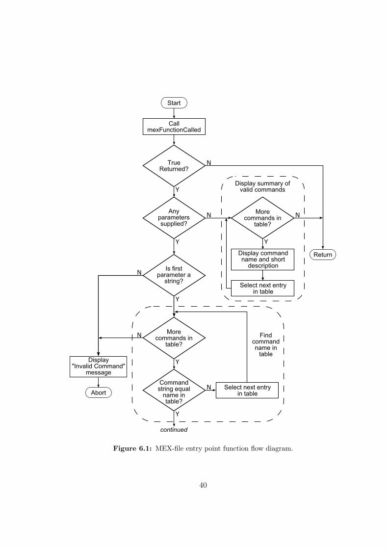
Figure 6.1: MEX-file entry point function flow diagram.

40

Figure 6.1: MEX-file entry point function flow diagram. (continued)

41

The resulting source code for this function, in addition to the showHelp and

l i n ewrapSt r ing functions, can be found in the files mex_dll_core.c and mex_

dll_core.h on the accompanying CD, as described in appendix G. The showHelp

function is used to display help information on each command, provided it is in-

cluded in the funcLookup array, whilst the l i n ewrapSt r ing function can be used

by any function that needs to format a string and display it in the MATLAB

command window.

The showHelp function’s overall structure is very similar to that of the entry point

function—initially the name of the function for which help is required is confirmed

to be a valid string, following which the command name is found within the lookup

table and, if the command is not found, an appropriate error is generated. If

the command name is found, the help for the command is displayed in three

stages. Initially the command definition is displayed listing the names of all input

and output parameters, generated from the command name and the parameter

names stored in paramrhs and paramlhs. Following this, using l i n ewrapSt r ing

the help text within the lookup table is displayed before lastly displaying all the

per-parameter information stored in paramrhs and paramlhs. By displaying the

help like this, it enables those who have just forgotten the order of parameters to

very quickly see the required list, whilst those who require more information can

read on further.

6.4 Testing

Before this core code could be used as part of the final utility it needed to be

tested. Although all parts were tested, it was the command dispatching code

that was most thoroughly tested because, unlike the rest of the code, any bug

here would affect the whole operation of the utility rather than just the display of

textual information.

42

Tests on the command dispatching included confirming that:

� the correct command function is called for the command name supplied, both

when using case-sensitive and case-insensitive string comparison.

� all parameters supplied in MATLAB are passed to mexFunctionCalled and

only the command parameters are passed to the required command function.

� various numbers of parameters can be returned, and all returned parameters

are correctly received in MATLAB.

� the minimum and maximum parameter number limits correctly stop the

command function from being called, and additionally that using a value of

-1 disables each limit.

� the correct behaviour is observed for both t rue and f a l s e return values from

both mexFunctionCalled and command functions.

� any incorrectly formatted entries in the funcLookup array, such as empty

or NULL strings and NULL function pointers, are handled gracefully.

Additionally, checks on the rest of the code included confirming that:

� the list of available commands correctly displays all commands.

� command help text is displayed correctly, even when including unexpected

but potential scenarios such as single words longer than the length of one

line. Also, correct tab alignment and line wrapping of lines including tabs

was checked.

� the list and descriptions of command input and output parameters displays

correctly, including scenarios where there are no parameters.

After fixing minor bugs these functions were accepted as being suitable for use in

the rest of the utility.

43

Chapter 7

Design of playrec MEX-file

Following the completion of the core MEX-file code, the specific implementation of

the utility was investigated. From previous tests, as described in chapter 4, it had

been decided that PortAudio should be used to provide the utility’s underlying

soundcard interface. Although this offered the synchronisation level required, the

utility still had to be designed carefully to ensure the channel timings did not drift

internally.

7.1 Request Pages

From the requirements specified, the utility could be pictured as a buffer between

MATLAB and the soundcard, or PortAudio in this case. Two common techniques

used when creating routines such as this to buffer audio data are to either use

a circular buffer or to double buffer the data. In both cases it is fairly easy to

maintain synchronisation between channels just by ensuring the same amount of

data is always added to all channels and similarly ensuring the same amount of data

is always removed from all channels. However, because of the initial requirement

not to have any predefined lifetime for recorded samples, such an approach would

not be suitable on its own because the samples would get overwritten unless the

44

buffers could grow indefinitely. Also, all unused channel buffers would have to

be zero filled, to keep them synchronised with the channels being used, and a

method to ‘mark’ where each record ‘request’ commenced would be required so

that the relevant recorded samples could be returned. Although it may have

been possible to use one of these techniques for output samples whilst using a

different approach for recorded samples, an alternative approach that grouped all

‘request’ information together was considered to be more reliable as well as easier

to maintain and debug should problems occur.

The resulting concept contained blocks, called pages, where each page represented

a single ‘request’ to the utility, no matter whether it was to record only, play only,

or to play and record simultaneously. Other key parts to this concept were:

� All channels used within the page start at the beginning of the page and the

length of each page is the same as the length of the longest channel of data

it contains.

� All pages are dynamically generated in memory when they are added. Al-

though this requires much more dynamic memory allocation than a circular

buffer or double buffer concept, it removes restrictions on the lifetime of

recorded samples and the number of pages that can be in the queue at any

one time.

� The minimum amount of space required by each page is used. All output

channels without samples are set to zero during the PortAudio callback,

avoiding the need to store and manipulate buffers just containing zeros. This

is also true for any output channels shorter than the length of the page.

Similarly, only the required input samples are stored.

� Pages are queued up end-to-end in the order they are added and are processed

with no gap between them.

� When there are no more pages in the queue, the utility waits for the next

page to be added, sending zeros to all output channels as required.

45

� When a page has finished, defined by the end of the page having been reached,

then all output samples are automatically removed from memory leaving only

the recorded samples and page-specific information. If the page contains

no recorded samples then the whole page is automatically removed from

memory. This is to reduce the amount of memory in use to a minimum

and to remove the need to manually remove any pages just used for sample

output.

� All pages are given a unique number to identify the page in all subsequent

uses of the utility, such as determining if the page has finished or requesting

the associated recorded data to be returned.

A diagram of three such pages, assuming the soundcard is configured to use 4 input

and 4 output channels, is shown in figure 7.1. This shows when output channels

are automatically zero padded as well as how continuous audio input or output

can be achieved provided the page is the same length as the channel buffer and

each page is added prior to the previous page finishing.

7.2 Thread safe design

Due to the PortAudio callback occurring in its own thread, the sharing of data

between the callback function and all other functions within the utility had to be

carefully designed. In this case, there were three main problem areas that had to

be considered: working with shared variables, how to add pages reliably, and when

to free memory.

From the MATLAB documentation[37] it was found that, even when using a

Graphical User Interface (GUI), all code is effectively executed in the same thread.

In the case when GUI events occur whilst another is being processed, the events

are either dropped or queued until a time when they can be processed. This occurs

when the previous event callback either finishes or calls one of a particular set of

46

Figure 7.1: Example arrangement of channel buffers within p lay rec pages for a sound-

card configured to use 4 input and 4 output channels. Black bars show

requested audio to be either played or recorded whilst grey bars show

times when output channels are automatically zero padded. Page 2 was

added prior to Page 1 finishing whereas Page 3 was only added after Page 2

finished.

47

functions including drawnow, pause or wa i t f o r . Thus, apart from the PortAudio

callback, no two functions within the MEX-file could be executed simultaneously

and therefore they would never interrupt each other. As such, the MEX-file could

be considered as using two threads—one for the PortAudio callback and one for

all other functions, called the main thread.

7.2.1 Shared Variables

When a variable is updated using a line of code such as tmpVar += 3, it cannot be

guaranteed that this will occur in one machine instruction, and so is not necessarily

atomic. For example it may take three instructions, read-modify-write, as shown

in the following disassembly:� �mov eax , dword ptr [ tmpVar (0FED9504h) ]add eax , 3mov dword ptr [ tmpVar (0FED9504h) ] , eax� �

Therefore it is possible that an interrupt could occur during the execution of this

line. Any changes to the value of tmpVar whilst this code is interrupted would

then initially have an effect, although when the code resumes the value of tmpVar

would be set to its old value plus 3, thus losing the other updates to the value.

Furthermore, if tmpVar is a large value spread across multiple memory locations it

is possible that its value could be read whilst it is half updated.

The simplest solution to this problem is to use variable types where the write

instruction is atomic, such as where a write requires only one machine instruction,

and ensure that the variable is only updated within one thread. With this, as many

threads as required can read the variable and they will never read an incorrect

value. Additionally, because only one thread writes to the variable no updates will

be lost. Due to its simplicity, this was the approach used wherever possible.

Sometimes more than one thread may need to update the same variable and so, to

ensure that no updates are lost, semaphores must be used so that only one thread

can access the variable at once. This means that each thread must block until no

48

other threads are accessing the variable. However, because of timing restraints on

the callback function, having it block would not be ideal and instead all thread

safety needed to be implemented without the callback blocking. One exception

to this requirement for semaphores is when a variable is only ever written rather

undergoing a read-modify-write cycle. In this case, provided only the latest value

to be written needs to be known, no problems will occur.

A further problem with sharing variables between threads is the uncertainty as

to when they might change due to the execution of code in an alternative thread.

This is most noticeable if the value of a variable is relied on as being constant

between the start and end of a function. In such scenarios, provided the variable

never needs to be updated, making a local copy for the duration of the function

avoids any problems.

When using multiple threads it is always imperative to ensure that no problems

due to shared variables will occur. This is because the independent timing of

threads means virtually no amount of testing can absolutely guarantee that there

are no problems. Furthermore, if any problems are found, they are often very

difficult to debug. Therefore, extra care must be taken to avoid this during the

initial design and implementation.

7.2.2 Adding Pages Reliably

To store all the pages in a queue, a linked list was to be used because of the ease

with which pages could be added and removed. To avoid potential problems due to

the use of multiple threads, even a basic operation such as this had to be carefully

considered. However, by ensuring that each page was completely generated before

adding it to the list, the list would never be incomplete and so there would not

be any possibility of a page being used by the callback before it was ready. (The

addition of an element to a linked list was confirmed to alter the list using a single

machine instruction, and therefore never place the list in an intermediate ‘corrupt’

state.)

49

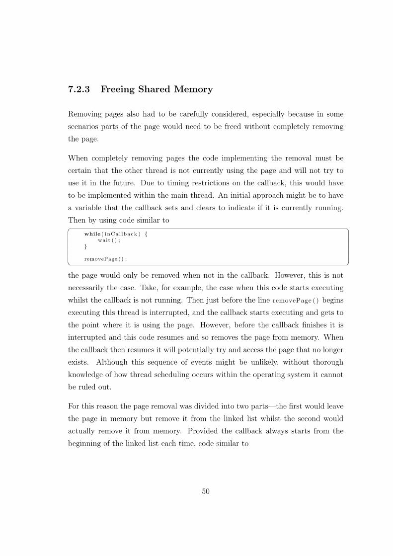
7.2.3 Freeing Shared Memory

Removing pages also had to be carefully considered, especially because in some

scenarios parts of the page would need to be freed without completely removing

the page.

When completely removing pages the code implementing the removal must be

certain that the other thread is not currently using the page and will not try to

use it in the future. Due to timing restrictions on the callback, this would have

to be implemented within the main thread. An initial approach might be to have

a variable that the callback sets and clears to indicate if it is currently running.

Then by using code similar to� �while ( inCa l lback ) {

wait ( ) ;}

removePage ( ) ;� �the page would only be removed when not in the callback. However, this is not

necessarily the case. Take, for example, the case when this code starts executing

whilst the callback is not running. Then just before the line removePage ( ) begins

executing this thread is interrupted, and the callback starts executing and gets to

the point where it is using the page. However, before the callback finishes it is

interrupted and this code resumes and so removes the page from memory. When

the callback then resumes it will potentially try and access the page that no longer

exists. Although this sequence of events might be unlikely, without thorough

knowledge of how thread scheduling occurs within the operating system it cannot

be ruled out.

For this reason the page removal was divided into two parts—the first would leave

the page in memory but remove it from the linked list whilst the second would

actually remove it from memory. Provided the callback always starts from the

beginning of the linked list each time, code similar to

50

� �removePageFromLinkedList ( ) ;

while ( inCa l lback ) {wait ( ) ;

}

removePageFromMemory ( ) ;� �guarantees that the callback will not use the page once it has been freed from

memory. This is because the page will only be removed from memory after a

period when the callback is not active, and therefore the next time the callback

occurs it will not have any ‘memory’ of the removed page.

This approach introduces two timing overheads. The first is the time taken for

the callback to iterate from the start of the linked list each time it is called. This

could be resolved by the callback storing an additional pointer to the last active

page so that each time the callback is called, it starts from this point in the linked

list. Although this would reduce the execution time of the callback, it would also

increase the complexity of removing pages, especially if the page being removed was

the page currently being used. Therefore, because the reduction in execution time

would only be noticeable if the linked list was very long, this timing overhead was

deemed acceptable compared to the increased complexity, and therefore potential

for problems, of the alternative approach. The second timing overhead is the delay

in the page removal code waiting for the callback to finish. In code that is trying

to continuously process data in the shortest time possible, having to wait for other

code to complete before continuing can be very costly. This is because the code is

suspended not only for the time until the other code finishes but additionally for

the time until the scheduler next runs the code. One solution would be to offer

page removal in two functions: one to remove it from the main linked list and

add it to a ‘to be deleted’ list, and a second to remove it from this ‘to be deleted’

list. Provided these functions were called far enough apart to ensure the callback

was not still using the pages to be deleted, this would avoid the need for any page

removal code to wait. However, this would increase the complexity of code both

within the utility and within MATLAB and therefore, because the slight timing

advantage was not deemed necessary, the simpler approach was used.

51

Ideally as much memory as possible should be freed as soon as it is no longer

required. This meant that play only pages could be deleted as soon as they had

finished. However, because page removal had to occur within the main thread it

would be very difficult to trigger this from within the callback and so an alternative

was required. One method would be to require all pages to be explicitly deleted

from within MATLAB. This would increase the time between a page finishing and

it being removed and would also not be intuitively obvious—sending samples to be

output from a soundcard, and then having to delete these samples after the output

has completed. Instead of this, the chosen method was to automatically free up

as much memory as possible each time the utility was used. This would slightly

increase the execution time of all utility calls but at the same time memory usage

would be kept to a minimum and, more importantly, the use of the utility would

be simplified. For all play only pages, the page would be completely removed from

memory (using the method above) whereas pages containing recorded samples

would have as much memory freed as possible whilst still leaving the page and

associated recorded samples in memory. To achieve this, a flag would be set by

the callback indicating the page was finished. Then, once this is set, the callback

must only use the page to access the next page in the linked list whilst the main

thread can alter the page as required, such as freeing up parts of memory, without

any concerns for thread safety. (For this to work correctly, the value of the finished

flag must never be altered in the main thread and also the pointer to the next item

in the linked list must be treated the same regardless of the state of the finished

flag.)

In addition to automatic page removal, to meet the utility requirements MATLAB

would need to explicitly remove pages. By checking that memory is not freed

twice, this could be implemented using the same command, based on the method

above, regardless of what play or record channels the page contained and whether

or not the page was finished.

52

7.3 Page Structures

To implement the page queueing using a linked list, pages were represented using

structures. The final design contains the three structures s t r e amIn f oS t ruc t t ,

s t reamPageStruct t and chanBufStruct t arranged as shown in figure 7.2.

Figure 7.2: Diagrammatic representation of the arrangement of s t r e amIn f oS t ru c t t ,

s t reamPageStruct t and chanBufStruct t structures used to contain all data

associated with a particular stream. This example is based on the first two

pages shown in figure 7.1. Note that any order of channels within the

chanBufStruct t linked list is acceptable and only the channels used need

to be included.

By grouping all data within a single top-level structure, s t r e amIn f oS t ruc t t ,

simultaneous support for multiple streams can be easily implemented should the

need arise. This structure contains stream specific information, such as sample

rate and the number of channels supported, as well as a pointer to the start of a

linked list of the ‘page’ structures s t reamPageStruct t . Each of these contains

53

page specific information, including the page number, and links to the start of up

to two further linked lists, one containing the buffers for the input samples whilst

the other contains the output sample buffers. These linked lists are constructed

using chanBufStruct t structures with one structure for each input and output

channel in the page. Using this approach it is very easy to represent a wide variety

of pages, even including different length buffers for each channel within the same

page.

The type definitions for these three structures, including descriptions of all the

variables, are shown in listing 7.1.� �typedef struct chanBufStruct tag {

SAMPLE * pbu f f e r ; // The channel audio dataunsigned int bufLen ; // Length o f the audio bu f f e runsigned int channel ; // Channel number on the audio dev i c e

// that t h i s bu f f e r i s a s s o c i a t ed with// ( f i r s t channel = 0)

struct chanBufStruct tag *pnextChanBuf ; // Pointer to the next channel// bu f f e r in the l i nked l i s t . The// order o f b u f f e r s in the l i nked l i s t// i s the order o f ' channel ' data// r e c e i v ed from and returned to MATLAB

} chanBufStruct t ;

typedef struct st reamPageStruct tag {chanBufStruct t *pf irstRecChan ; // F i r s t record channel with in t h i s pagechanBufStruct t * pf i r s tPlayChan ; // F i r s t play channel with in the page

unsigned int pageLength ; // The length o f the page ( in samples )volat i le unsigned int pagePos ; // The cur rent p o s i t i o n with in the pageunsigned int pageNum ; // A unique id to i d e n t i f y the page

unsigned int playChanCount ; // The number o f channe l s used to communicate// with PortAudio . Must be g r e a t e r than// the maximum channel number used .

bool *pplayChansInUse ; // Pointer to array type bool , s i z e playChanCount .// Each element can be :// t rue − the channel i s in the play l i nked l i s t// f a l s e − the channel i s not in l i nked l i s t// Se t t i ng f a l s e means that the channel i s s e t// to a l l z e r o s with in the ca l l ba ck . Any channe l s// not inc luded in t h i s l i s t ( or s e t t rue ) must// be inc luded in the play channel l i nked l i s t .

volat i le bool pageUsed ; // Set t rue i f the page has been used in the// PortAudio ca l l b a ck func t i on

volat i le bool pageFinished ; // True i f the page has been f i n i s h e d ( a l l r ecord// bu f f e r s f u l l and a l l output bu f f e r s 'empty' )// Once set , t h i s and pnextStreamPage are the// only v a r i a b l e s the PortAudio ca l l b a ck w i l l read// ( none are wr i t t en )

struct st reamPageStruct tag *pnextStreamPage ;// The next page in the l i nked l i s t

} s t reamPageStruct t ;

54

typedef struct {s t reamPageStruct t * pf i r s tStreamPage ; // F i r s t page in the l i nked l i s t

PortAudioStream *pstream ; // Pointer to the stream , or NULL f o r no stream

t ime t streamStartTime ; // The s t a r t time o f the stream , can be used to// determine i f a new stream has been s t a r t ed .

// Conf igurat ion s e t t i n g s used when opening the stream − s e e Pa OpenStream// in portaudio . h f o r d e s c r i p t i o n s o f the se parameters :double sampleRate ;unsigned long f ramesPerBuf fer ;unsigned long numberOfBuffers ;PaStreamFlags streamFlags ;

volat i le bool stopStream ; // Set t rue to t r i g g e r the ca l l b a ck to stop the// stream .

volat i le bool inCa l lback ; // Set t rue wh i l s t in the ca l l b a ck .

volat i le unsigned long skippedSampleCount ;// The number o f samples that have been zeroed// wh i l s t the re are no un f i n i sh ed pages in the// l i nked l i s t . Should only be modi f i ed in// the ca l l ba ck . Use resetSkippedSampleCount// to r e s e t the counter .// I f resetSkippedSampleCount i s t rue the value// o f skippedSampleCount should be ignored and// in s t ead assumed to be 0 .

volat i le bool resetSkippedSampleCount ;// Set t rue to r e s e t skippedSampleCount ( the r e s e t// takes p lace with in the ca l lback , at which po int// t h i s i s c l e a r ed ) . Because both s e t t i n g and// c l e a r i n g t h i s are atomic ope ra t i on s the re i s// no p o s s i b i l i t y a r eque s t to r e s e t can be// missed .

volat i le bool i sPaused ; // s e t t rue to 'pause' playback and reco rd ing// Never s tops the PortAudio stream , j u s t a l t e r s// the data t ransmit ted .

PaDeviceID playDeviceID ; // Device ID f o r the dev i c e being used , or// PaNoDevice f o r no dev i c e

PaDeviceID recDeviceID ; // Device ID f o r the dev i c e being used , or// PaNoDevice f o r no dev i c e

unsigned int playChanCount ; // The number o f channe l s used to communicate// with PortAudio . Must be g r e a t e r than// the maximum channel number used .

unsigned int recChanCount ; // The number o f channe l s used to communicate// with PortAudio . Must be g r e a t e r than// the maximum channel number used .

} s t r e amIn f oS t ru c t t ;� �Listing 7.1: Type definitions for s t r e amIn f oS t ru c t t , a structure used to group all

data associated with a particular PortAudio stream, s t reamPageStruct t ,a structure used to group all data associated with a particular page, andchanBufStruct t , a structure to store a single channel of data.

55

Within this set of structures there are a few important variables not previously

mentioned. The first of these are pagePos combined with pageLength within

s t reamPageStruct t . When a page is constructed, pageLength must be set to

the length of the page which, unless a gap is required at the end of the page, must

be the same as the length of the longest channel. The single variable pagePos is

then used to store the current sample position within the page, making it impos-

sible for the channels within a page to ever be temporally mis-aligned within the

utility. Through a simple comparison between these two values it is also possible

to determine how many samples still need to be processed in the page, avoiding

the need to find the length of the longest buffer each time the page is used. Prob-

lems indexing beyond the end of each channel buffer can also be easily avoided by

comparing the page position with the buffer length stored with each channel.

Two further important variables are playChanCount and pplayChansInUse within

s t reamPageStruct t . The first of these is used to store the size of the second to

ensure indexing outside the array does not occur and, until the page has finished,

should be the same as the variable with the same name in s t r e amIn f oS t ruc t t .

pplayChansInUse is used within the PortAudio callback to indicate which output

channels need to be zeroed due to not having an associated buffer of samples. Two

alternative approaches to this would be to either zero all output samples at the

start of the callback or to generate this list of used channels within the callback each

time. The former would needlessly increase the processing time of the callback,

especially if a large number of channels are in use and the page contains data for

all channels, whilst the latter would require dynamic memory allocation within

the callback, something which should be avoided due to the potential time it may

require.

The final variable that requires further mention is stopStream within

s t r e amIn f oS t ruc t t . This is required because, as mentioned in appendix B,

although Pa StopStream ( ) can be used to stop the PortAudio stream, problems

can be encountered freeing memory directly following this. As an alternative,

when this variable is set the callback stops the stream by returning a specific

56

value. By setting this variable and then waiting for the stream to stop before

continuing, problems freeing memory are avoided.

7.4 Implementation

Based on the requirements to ensure thread safety, the functions to run in the main

thread were designed. For the majority of these, one function was used for each

command to be called from within MATLAB. However, to improve the structure

of the code, some additional ‘helper’ functions were also written. These included

functions to:

� create new instances of the s t r e amIn f oS t ruc t t and s t reamPageStruct t

structures, allocating the required memory and setting all the contained

variables to their defaults. Although each of these is only called from one

place within the utility, this neatly grouped all default values together making

them easy to locate and change as necessary.

� remove structures from memory, making sure that all memory is only freed

once and all necessary precautions are taken as outlined above.

� check the current state of the utility compared to that required, generating

an appropriate error if required, such as when trying to add a page before

the utility has been initialised.

� condense all pages that have finished, as described above.

� check the error code returned by all PortAudio functions, displaying the error

number and description if an error has occurred.

Apart from these ‘helper’ functions and the functions specific to each command,

three further functions also had to be implemented. These were:

57

mexFunctionCalled the function called by the core MEX-file code whenever the

utility is used. This determines if the utility had been used before, and if

not initialises PortAudio and registers the exit function exitFunc . This also

calls the helper function used to condense all pages.

exitFunc the function to be called by MATLAB when either MATLAB is closed

or the utility is cleared from memory. This ensures that all dynamically

allocated memory is freed correctly, that the PortAudio stream is stopped

and that PortAudio is terminated.

playrecCallback the callback function for PortAudio. This transfers all sample

data between the utility’s page structures and PortAudio, based on the flow

diagram shown in figure 7.3.

The resulting source code for these functions, in addition to all other code spe-

cific to the operation of the utility, can be found in the files pa_dll_playrec.c

and pa_dll_playrec.h on the accompanying CD, as described in appendix G.

Additionally, a list of all of the commands implemented by the utility to meet

the requirements can be found in appendix D along with their descriptions as re-

turned by the ‘help’ command and a complete overview of the utility’s operation

as returned by the ‘about’ command.

7.5 Testing

Although the core MEX-file code had already been tested, when testing the utility

as a whole many of the tests had to be repeated to ensure that the funcLookup

array had been implemented correctly, such as including the correct limits on the

number of parameters. Tests like this, as well as checking for the correct return

values from commands, were specifically implemented. However, to test for correct

operation it was decided that this should predominantly occur through using the

utility in real scenarios. This decision was made for two reasons. The first was the

58

Figure 7.3: PortAudio callback function flow diagram.

59

extra time already taken developing the utility, and so the reduced time available

to complete the remainder of the project. The second was the likely nature of

any bugs that might exist: after initial testing for underlying correct operation—

such as testing continuous input and output, pausing and resuming, page list

generation and correct explicit and automatic removal of pages from this list—any

bugs potentially remaining would most likely be due to either incorrect dynamic

memory (de)allocation or unexpected ‘interaction’ between threads, both of which

are best found through extensive use of software.

Examples of the specific tests implemented included:

� confirming each command correctly accepted its valid range of parameters

whilst rejecting both one more and one less, where applicable, than this

range. Due to the testing of the MEX-file core code, further testing outside

this range was not conducted.

� confirming the list of commands displayed all available commands, and the

help information for each command displayed as expected based on the text

entered into the funcLookup array.

� confirming that audio output across multiple pages was continuous, contain-

ing no audible glitches. This was implemented by outputting a sine wave

across multiple pages. To confirm the correct samples were always being

used, the period of the sine wave, the page size and the callback frame size

were all set to be non-integer multiples of each other. Additionally, varying

page sizes and different frequencies on each channel were tested.

� confirming that audio recording across multiple pages was continuous, con-

taining no audible glitches. To test this, sine waves, as used to test the

output, were looped back to the input channels. Through listening to these

recoded signals, any glitches in recording would be heard.

� confirming correct operation of automatic page removal, explicit page re-

moval and page list generation. This was tested by rapidly adding a group

60

of pages—some just to record, some just to play and some to do both—to the

utility in a pseudo-random order. Then whilst these pages were processed

the page list returned by the utility would be monitored, ensuring that only

the play only pages were automatically removed. Further to this, correct

operation was tested when all three types of pages were deleted in all three

possible states: prior to starting being processed, whilst they were being

processed, and after they had finished being processed.

� confirming that appropriate warnings and errors were displayed when channel

lists were used either containing duplicated channel numbers or channels out

of the range specified during initialisation. Additionally, correct warnings

were confirmed for scenarios when the number of output channels of data

and the list of output channels to use were of different sizes.

One further test was to repeat the loop back tests initially conducted using the

standard MATLAB audio functions and pa wavplay, as described in chapter 4.

Through the use of consecutive combined play and record pages this would test if

the relative timings of the inputs and outputs remained the same over prolonged

periods of time. Unexpectedly, since no glitches had been found in previous testing,

the delay was found not to remain constant. On most occasions during this testing

the recording always preceded the output by 584 samples, although sometimes this

started at 579 samples before changing to 584 samples during the test. Whenever

the delay started at 579 samples, this change was always found to occur, although

the time between initialising the utility (the utility was re-initialised before each

test commenced) and the change occurring did not seem to have any pattern

taking from seconds through to minutes. Instead, it was found that the change

could sometimes be ‘triggered’ through significantly increasing hard-disk access

and processor usage, such as starting a new application. It was surmised that the

relatively short durations of the original ‘continuous output’ and ‘continuous input’

tests were not long enough to observe this behaviour, which is why no problems

were found initially.

Importantly, it was found that the change in delay would only ever occur once,

61

after which the relative timings would remain constant—two tests each of over

12 hours demonstrated this.

As when testing the pa wavplay utility, the delay was found to be the same on

all channels. Therefore, by connecting an external signal generator to one input

whilst recorded a loop back signal on another, the origin of the delay change could

be narrowed down. The two resulting signals during a change in delay are shown

in figure 7.4, showing that the 5 extra samples are added to the output signal, as

expected by the glitch heard in the output sine wave.

5550 5600 5650−1

−0.8

−0.6

−0.4

−0.2

0

0.2

0.4

0.6

0.8

1

Sample Number

Sam

ple

Val

ue

Figure 7.4: Comparison of a looped back sine wave (solid line) and an externally gen-

erated sine wave (dashed line) during a change in delay when using the

playrec utility. This shows how only the looped back signal is affected

during the change, and therefore the extra samples all occur within the

output.

62

After continued testing, neither the pa wavplay utility nor the initial functional

test code could be made to reproduce this problem. However the results measured

during the initial testing of the pa wavplay utility, as described in chapter 4, were

seen to indicate that this change may occur, although very occasionally compared

to that with the playrec utility. To try and explain the cause of both these infre-

quent variations when using the pa wavplay utility and the change of delay within

the playrec utility, the effect of various different changes were investigated. This

included restarting the computer multiple times to determine if there are varia-

tions in how the soundcard initialises itself as well as using different sample rates

and numbers of channels to determine if the problem may be due to the soundcard

configuration. None of these provided any clues to the cause of the problem and

instead just revealed that there was no absolute guarantee what delay between out-

put and input would ever occur. Also, as before, the delay measured was always

the same on all channels.

Due to the use of a single variable to store the position within each page, it was

realised that the change in delay could not be occurring within the utility. However,

this did not rule out the utility inadvertently triggering the change. If this was the

case, the most likely cause would be the execution time of the PortAudio callback

although various tests, including adding delay loops into the callback, did not

reveal any connection between this and the delay changes. This was not surprising

because, if this was the trigger, the change in delay would be expected to occur

on more than one occasion.

Although a large amount of further testing and investigation into the operation of

PortAudio and Steinberg’s ASIO SDK may have found the cause of this problem,

this was expected to take a long time with potentially no solution at the end,

especially if the problem was hardware related. Therefore, instead, the fact that

the change in delay only ever appeared to occur once was utilised and a MATLAB

function was written to monitor the latency between an output and input until a

predetermined ‘stable’ delay was measured. Although not ideal, using this before

all subsequent testing would allow the rest of the project to continue and, by

63

ensuring a loop back signal was always recorded during all tests, the delay between

output and input could be checked later on should anomalies appear. Furthermore,

by trying to run as many tests as possible without restarting either MATLAB or

the playrec utility, the possibility of this causing any problems would be reduced.

64

Chapter 8

Excitation Signals

To measure the distance between a sound source and microphone, the time-of-

flight, t (s), of a sound between them can be used along with the speed of sound

in air, c (ms−1), to give the separation as

d = ct (m). (8.1)

The speed of sound in air can be approximated by

c = (331.5 + 0.6T ) (ms−1) (8.2)

where T is the air temperature in degrees Celsius. In order to use this approach an

accurate method of determining the time-of-flight is required. Approaches using

a single stationary microphone require a known signal, the excitation signal, to

be transmitted at a known time, and the processing of the recorded microphone

signal to determine when the sound arrives. Many different signals can be used,

although each has its own advantages and disadvantages. This chapter considers

the suitability of different signals before providing implementation details for those

signals to be used in all tests.

65

8.1 Signal Types

8.1.1 Pulsed Sine Wave

This is the simplest form of excitation signal and through the use of a matched

filter can provide a high Signal-to-Noise Ratio (SNR). However, due to the signal’s

repetitive nature it is only possible to measure the relative phase between loud-

speaker and microphone. Hence the actual separation could be one of an infinite

number of values, separated by multiples of the signal wavelength. By determin-

ing the relative start and end times of the received signal the measured separation

could be reduced to a much smaller subset of values, although not necessarily to

just one. However, if room reflections sum together to give a signal 180◦ out of

phase with the direct sound then it is possible that the microphone would not

receive the signal at all. Although this is unlikely, a much more likely scenario is

for the reflections to add such that the phase of the received signal is different from

that solely of the direct signal. As such, the only reliable measurement of phase

would be that made before any reflections reach the microphone—something diffi-

cult to achieve, especially in a normal environment where the loudspeakers may be

placed against a wall or even in a corner. Through the use of more than one signal

frequency the problems of having an infinite number of potential separations can

be reduced or eliminated, although the requirement to measure the relative phase

before the first reflection arrives still exists, making this approach impractical.

8.1.2 Impulse

The use of an impulsive signal enables the impulse response (IR) for a particular

arrangement of loudspeaker and microphone to be measured. From this it is pos-

sible to determine the relative separation by determining the time for the direct

signal to be received. Although, as with the sine wave, room reflections will in-

terfere with the received signal this does not happen until after the direct signal

66

has been received, and so can be ignored without any problems. However, because

impulses from loudspeakers can only contain relatively small amounts of energy,

such an approach can be very susceptible to even small amounts of background

noise, making it difficult to identify the impulse from the noise. To try and remove

this problem, multiple measurements can be taken and averaged. This requires a

long enough time to be left between repeats to ensure that the previous impulse

has completely decayed away, and even then may require many repeats to obtain

an accurate result.

8.1.3 Maximum Length Sequence (MLS)

As with an impulse excitation signal, the IR of a room can be measured using a

Maximum Length Sequence (MLS). However, this technique is much less suscep-

tible to background noise than the impulse case. An mth-order MLS is a pseudo

random signal of length L = 2m− 1 samples, which can be generated using a shift

register by exclusively or-ing particular registers, as shown in figure 8.1[33]. The

resulting signal is periodic with period L samples which can then be scaled as

required to obtain the loudspeaker signal.

Figure 8.1: Example 4th-order binary Maximum Length Sequence (MLS) generation

using a shift register.

After the response of a linear time-invariant system, such as a room, to this signal

has been measured the IR can be determined in two different ways. The first uses

circular correlation[34] whilst the second uses the Hadamard transform[19]. In

both cases, the same result is obtained.

Importantly, the Fourier Transform of the original MLS has the same magnitude

for all frequencies, apart from the dc component, whilst the phase is effectively

67

randomised. This results in extraneous noises within the room being uniformly

distributed along the resulting IR (provided the noise has a white spectrum)[34],

meaning the technique is particularly suited to scenarios where people may be

in the room and moving around. However, this technique does also exhibit vari-

ous disadvantages, the most significant of which are distortion peaks due to non-

linearities in the system, such as within the loudspeaker[41]. Additionally, if the

length of the MLS is shorter than that of the IR for the room, time-aliasing occurs

with the ‘tail’ of the IR appearing overlaid on the start of the actual IR[34].

8.1.4 Inverse Repeated Sequence (IRS)

Based on a MLS, an mth-order Inverse Repeated Sequence (IRS) has length 2L

samples and can be generated using the equations[34]

IRS[n] =

{MLS[n], n even

−MLS[n], n odd. (8.3)

In this case only circular correlation can be used to deconvolve the IR from the

measured room response to the IRS[10, 34]. This technique has been shown to

have “complete immunity to even-order nonlinearity while maintaining many of

the advantages of MLS”[6]. However, it does require twice as long an excitation

signal to be used compared to using an MLS because, to avoid time-aliasing, L

must still be longer than the IR length.

8.1.5 Optimum Aoshima’s Time-Stretched Pulse (OATSP)

The concept of using a Time-Stretched Pulse (TSP) to measure the IR of a linear

system was introduced by Aoshima[1]. In this, an impulse signal with a near flat

power spectrum undergoes expansion by applying a phase shift to each frequency

component in the frequency domain. The resulting signal has the same total energy

as the original impulse although it has a much smaller maximum amplitude in the

68

time domain. Therefore the whole signal can be increased in amplitude and so the

final excitation signal can contain much more energy than the original impulse,

and so significantly increase the SNR. By applying the opposite phase shift to each

frequency component within this signal, the original impulse, albeit much larger,

can be obtained. Similarly, if this opposite phase shift is applied after the TSP

has been passed through the linear system, the IR of the system can be obtained.

As an extension of the single specific example given by Aoshima, Suzuki et al [36]

proposed the “Optimum” Aoshima’s Time-Stretched Pulse (OATSP), specified in

the frequency domain as

H[k] =

exp(

j4mπk2

N2

), 0 ≤ k ≤ N

2

H∗[N − k], N2< k < N

(8.4)

with the inverse, deconvolution, filter given by

H−1[k] =

exp(

−j4mπk2

N2

), 0 ≤ k ≤ N

2

H−1∗[N − k], N2< k < N

(8.5)

or more simply

H−1[k] =1

H[k]

where m is an integer determining the ‘stretch’ of the OATSP and N is the signal

length.

(In [36], (8.4) and (8.5) are given without the complex conjugate for N2< k < N ,

although this is necessary to obtain a real time domain signal.)

The excitation signal can be obtained by taking the Inverse Discrete Fourier Trans-

form (IDFT) of (8.4). Then, provided the IR is shorter than N samples, circular

convolution of the system’s response to this signal with the inverse filter will re-

sult in the system’s IR. Furthermore, if the IR is longer than N samples, the

time-domain excitation signal and inverse filter can be circularly rotated by

nrot =N

2−m (samples)

before being extended with zeros to make the total signal length longer than the

IR. In this case linear convolution must then be used to obtain the IR[36].

69

8.1.6 Logarithmic Sweep

The logarithmic sweep excitation signal, unlike the other excitation signals dis-

cussed, contains the same energy per octave. This is achieved by ensuring “the

frequency increases with a fixed fraction of an octave per unit time”, such that

log(

f2

f1

)T2 − T1

= constant

where f1 is the frequency at time T1 and f2 is the frequency at time T2[23]. This

has the advantage that a higher proportion of the excitation signal energy is at

lower frequencies, and so the SNR for these frequencies will be improved.

Additionally, using this technique “each harmonic distortion packs into a separate

impulse response” in the deconvolved signal, at points prior to the linear IR of

the system. As such, the system’s linear IR can be separated from any distortion

artefacts[8].

Unlike the OATSP, the logarithmic sweep can be generated in the time domain

using the equation

x(t) = sin

ω1T

ln(

ω2

ω1

) (exp

tT

ln“

ω2ω1

”−1

) (8.6)

where ω1 is the starting frequency, ω2 is the ending frequency and T (seconds)

is the duration of the sweep. The inverse filter, with which the room’s response

can be convolved to obtain the IR, is then generated by “time-reversing the ex-

citation signal, and then applying an amplitude envelope to reduce the level by

6 db/octave”[8].

Another advantage of this technique is that, as with OATSP, the sweep does not

need to be longer than the IR and instead it can be extended with silence to

measure longer IRs. If the resulting signal is still not long enough, time-aliasing,

as would occur with both MLS and IRS, does not occur and instead the end of

the IR is just ‘lost’[8].

70

8.1.7 Summary

A comparison of the four excitation signals MLS, IRS, OATSP and logarithmic

sweep was conducted by Stan et al in [34]. From this it was concluded that the

noise immunity of both MLS and IRS made them more suited to measurements

in “an occupied room or in the exterior” and additionally these excitation signals

were “more bearable and more easily masked out”. However, these signals required

much more calibration to obtain optimum results and exhibited distortion peaks,

something not present when using either of the other signals. OATSP was found

to perform best at high output signal levels to reduce the SNR, although this was

said to make it “unusable in occupied rooms”. Finally, the logarithmic sweep was

found to be “the best impulse response measurement technique in an unoccupied

and quiet room” even though it did not require “tedious calibration”.

Based on this assessment, none of these signals is best for all of the conditions under

which the loudspeaker locations would ideally be measured—that of an occupied

room where the signal level does not require any manual calibration and ideally

very little automatic calibration. For this reason, in addition to determining if the

direct sound ‘peak’ in the IR appears differently using the different techniques, all

four techniques were investigated.

8.2 Signal Creation and Processing

Although the excitation signals to be tested required different algorithms to both

create the excitation signal and process the recorded signal, the process of playing

and recording would be the same in all cases. Additionally the same excitation

signal would be used many times, and so to speed up the analysis as many cal-

culations as possible associated with the post-processing stage were moved to the

signal creation stage, thus ensuring they only had to occur once. To achieve this,

an easy and generic method of keeping track of the excitation signal and recorded

signal(s) as well as information about the type of signal was required.

71

The chosen method was to use three variables within MATLAB: first, a vector

for the excitation signal; second, a vector or matrix for the recorded signal(s), of

a length equal to or greater than the excitation signal; and third, a ‘parameters’

structure. This contained all the relevant information about the type of signal

being used including one ‘type’ field indicating the type of signal, and hence the

function that must be used to process it. With this approach, the function to create

each test signal would return the excitation signal and the parameters structure

whilst the function to process the recorded signal would just take the recorded

signal and the associated parameters structure. Based on this, four c r e a t e and

four p ro c e s s functions were implemented, each ending in either mls, i r s , oatsp or

sweep to indicate the excitation signal type they created and processed respectively.

Additionally a generic p r o c e s s r e c o rd i n g function was created to call the relevant

p ro c e s s function, based on the contents of the supplied parameters structure.

The files containing these functions can be found on the accompanying CD, as

described in appendix G.

8.2.1 Maximum Length Sequence (MLS)

To create the MLS excitation signal three parameters were required:

sequence order, m, which is the same as the size of the shift register required

and from which the period of the sequence, L = 2m − 1, can be determined.

The shift register taps given by Vanderkooy[41] were used to generate the

MLS due to their suggested improvement in performance compared with

other possible combinations. Using these, a binary MLS between 0 and 1

was generated using code as shown in listing 8.1.

Although, provided at least one bit is set, the shift register can start in any

state, a start state with all bits set was always used for consistency.

repeat count to specify how many times the length L sequence should be re-

peated, which can be used to improve SNR through averaging during anal-

72

ysis. However, due to the use of a circular deconvolution method, either the

system response during the first repeat should be excluded from the analysis

or the system response after the last repeat should also be included in the

averaging process.

signal scaling to specify the values between which the MLS should switch. To

create a symmetrical signal about zero, this was specified as a single scaling

factor such that the sequence used the values ±scaling.

� �L = 2ˆmorder − 1 ;

% Create morder−b i t bitmask and s e t the s h i f t r e g i s t e r ( s r ) s t a r t s t a t ebitmask = bitcmp ( uint32 (0 ) , morder ) ;s r = bitmask ;

% Create a p lace to s t o r e the output sequence from the s h i f t r e g i s t e r ,s rout = in t8 ( zeros (1 ,L) ) ;

for i = 1 :Ls rout ( i ) = b i t g e t ( sr , morder ) ;s r = mod(sum( b i t g e t ( sr , taps ) ) , 2) + bitand ( b i t s h i f t ( sr , 1) , bitmask ) ;

end� �Listing 8.1: MATLAB implementation of a shift register of order morder, where taps

already contains the required tap numbers, as given in [41], in a row vector.

In principle circular correlation could be used to deconvolve this signal. However,

due to the fact that the signal length was not a power of two and was also large,

implementing this in either the time or frequency domain could be very time

consuming, especially when compared to using the Fast Hadamard Transform

(FHT). For this reason the FHT was used, and as a result two further vectors were

created whilst creating the MLS—one to reorder the samples prior to implementing

the transform and a second to reorder the output of the transform. These were

generated in a similar manner to [19]: the first can be generated using the shift

register value as each sample is shifted out. The second, however, is generated

in two stages—first the occasions when only one bit is set in the shift register

are determined (that is, contains a value which is a power of two) and then this,

combined with the values in the original sequence, is used to determine the second

reordering vector.

73

Through storing these reordering vectors within the ‘parameters’ structure, the

process of deconvolving the room’s response is greatly simplified:

1. A number of repeats of the recording are averaged to obtain a single sequence

L samples long. To allow comparisons between the averaging of different

numbers of repeats, the range of repeats to average could be specified when

calling the MLS processing function.

2. The averaged samples are reordered according to the first reordering vector,

including the addition of an extra, zero, sample at the start.

3. The FHT is applied. Different methods of implementing this were evaluated

including one that applied the transform on the data in-place[19], whilst

another required enough space to storem+1 times the length of the MLS[17].

The final method chosen was based on the latter, but only requiring two

buffers by bouncing the data between them. This was chosen due to the

longer execution time of the in-place method within MATLAB, a result of

requiring multiple nested loops.

4. The processed samples are reordered according to the second reordering vec-

tor, including the removal of the first sample, and scaling as appropriate.

The resulting signal contains the room’s IR starting at the first element.

8.2.2 Inverse Repeated Sequence (IRS)

To create this signal, initially an unscaled MLS was required, generated as de-

scribed above. Following this, the IRS was generated using (8.3) before it was

repeated and scaled in exactly the same way as for the MLS. However, due to the

need to use circular correlation to deconvolve this signal, no further variables had

to be created at this stage.

The processing of this signal was no more complicated than its creation—averaging

of multiple repeats, as described above, and then calculating the circular corre-

74

lation between this averaged signal and the original IRS. The resulting signal

contains the room’s IR starting at the first element with an inverted version of the

IR starting after L samples.

8.2.3 Optimum Aoshima’s Time-Stretched Pulse (OATSP)

When creating an OATSP more parameters needed to be specified than for either

the MLS or IRS. These were the OATSP length, N , the stretch factor, m, the

length to extend the OATSP with zeros, the number of repeats of the signal, and

the scaling factor (the required peak value). The most complicated of these is m,

which can have significant impact on the error caused by using linear convolution

instead of circular convolution[36] as well as on the amount of energy within the

signal, and hence the SNR. For example, at one extreme, when m = 0, an impulse

is obtained which contains very little energy but which would introduce no error

when processed with linear convolution. In comparison, when m approaches, and

is greater than, N2, the signal can contain far more energy than the impulse but

the tail of the signal ‘wraps around’ onto the start, introducing a significant error

when using linear convolution.

One way to determine an appropriate value for m is to calculate the value which

introduces an error which is just below that required, such as -98 dB, the equivalent

dynamic range of 16 bit quantisation[36]. For this reason, two functions in addition

to c r e a t e oa t s p were created—one to calculate the average or maximum error due

to using linear convolution, oatsp CalcPowErr, and a second to find the value of

m to obtain a particular error, oatsp FindPowErr.

Having determined the required value for m, the unscaled OATSP was generated

using the code shown in listing 8.2. To obtain the required excitation signal, this

time domain signal was then scaled, extended at the end with zeros and repeated

according to the specified values. The final inverse filter was created by adding

the same number of zeros to the start of the time domain signal before scaling by

the same factor.

75

� �n1 = 0 :N/2 ;n2 = (N/2+1) : (N−1) ;

H(n1+1) = exp( j *4*m*pi*n1 .ˆ2/Nˆ2) ;H(n2+1) = conj (H(N − n2 + 1) ) ;

G=1./H;

ro t = N/2 − m;

h = c i r c s h i f t ( real ( i f f t (H, N) ) , [ 0 , −ro t ] ) ;g = c i r c s h i f t ( real ( i f f t (G, N) ) , [ 0 , r o t ] ) ;� �Listing 8.2: Creation of an Optimum Aoshima’s Time-Stretched Pulse (OATSP) of

length N and stretch m using MATLAB, generating both the time (h andg) and frequency (H and G) domain representations of both the excitationsignal (h and H) and inverse filter (g and G).

To process the resulting recorded signal, it was initially averaged over multiple

repeats before being windowed with a Tukey window to reduce the errors when

applying a DFT. This was then linearly convolved with the ‘extended’ inverse filter

to obtain the IR, which started in the middle of the resulting signal in the sample

after the length of the ‘extended’ excitation signal.

8.2.4 Logarithmic Sweep

Initially two different methods were investigated for creating the logarithmic sweep.

The first worked in the time domain, as given by (8.6), whilst the second worked in

the frequency domain, as described by Muller and Massarani[23]. The advantage

of the latter is reduced ripple in the magnitude spectrum, although in the time

domain this was found to produce more than one frequency at any one point in

time and as a result would not enable the linear IR to be measured without the

effect of harmonic distortion, as described by Farina[8].

To generate a logarithmic sweep within MATALB, the ch i rp function from the

Signal Processing Toolbox can be used, provided an initial phase of -90◦ is specified

such that the signal starts at zero. This signal must be windowed, to avoid errors

due to transients at the ends of the signal, and scaled before being repeated as

76

required. The inverse filter can then be generated following the steps quoted in

section 8.1.6.

To obtain the IR, exactly the same process was used as for the OATSP: average,

window and then linearly convolve. However, in this case the first sample of the

linear IR was at the length of the excitation signal, not the sample after it.

8.2.5 Testing

Whilst creating all the required files to generate and process these different exci-

tation signals, their performance was compared with that expected. This included

analysing both the time and frequency domain representations of all excitation

signals and inverse filters, where applicable, as well as confirming that an impulse

is obtained when each excitation signal is processed directly. Further to this, each

excitation signal was linearly convolved with an imaginary room IR before decon-

volving to obtain the IR. The resulting IR was then compared to that convolved

with the excitation signal, confirming if the functions were operating as required.

Finally, to check the logarithmic sweep was implemented correctly harmonic dis-

tortion was added to the excitation signal prior to processing. The resulting IR

was then visually inspected to ensure each order of harmonic distortion had packed

into its own IR prior to that of the linear IR.

8.3 Test Implementation

As it would not have been possible to investigate the impact on measurement

accuracy of every excitation signal parameter, a set of excitation signals to be

used in all tests were specified. These all used a sample rate of 44100 samples/s,

and were defined as follows:

MLS A 16th-order MLS giving L = 65535 and so a duration of approximately

77

1.5 s, ensuring time-aliasing would have minimal effect. This was repeated

five times to allow signal averaging.

IRS A 16th-order IRS giving L = 65535, and therefore a signal period of approxi-

mately 3.0 s. This was repeated three times to allow signal averaging whilst

maintaining an overall signal length comparable to that of the MLS.

OATSP1 An OATSP with length N = 212 = 4096 and 90% stretch factor giving

m = 1843, padded with 216 − 212 = 61440 zeros and then repeated 5 times.

The zero padding in this signal, as with OATSP2, was included so that all

OATSP excitation signals had the same period, thus allowing a comparison

between different values of N . A 90% stretch factor was greater than that

used in [34] but still corresponded to an average power error from using

linear convolution of approximately -101.3 dB, so was used to increase the

total signal power.

OATSP2 An OATSP with length N = 214 = 16384 and 90% stretch factor giving

m = 7373, padded with 216 − 214 = 49152 zeros and then repeated 5 times.

OATSP3 An OATSP with length N = 216 = 65536 and 90% stretch factor giving

m = 29491, repeated 5 times.

Sweep1 A logarithmic sweep with length N = 216 = 65536, start frequency

f1 = 10 Hz and end frequency f2 = 22000 Hz. This is the same as that used

in [34], although in this case the signal was repeated five times so that all

the excitation signals were of similar length.

Sweep2 A logarithmic sweep with length N = 218 = 262144, start frequency

f1 = 10 Hz and end frequency f2 = 22000 Hz. This excitation signal was

included to allow a comparison between averaging a repeated signal and using

no averaging for a signal of similar total length. Theoretically, avoiding the

use of multiple averages solves problems associated with measuring slightly

time-invariant systems[8].

78

The amplitude of each of these signals was set by measuring the level recorded when

each signal was directly looped back. This ensured that any overshoot that may

have occurred due to filtering within the soundcard would not introduce distortion

caused by clipping[23]. The scaling factors used were 0.4 for the MLS and IRS

signals and 0.9 for all other signals.

Every time an excitation signal was used in a test, the excitation signal, recorded

signals and parameters structure were saved to a new file along with specific infor-

mation about the test, such as the loudspeaker-microphone separation and their

relative angles. Including the excitation signal and parameters structure in every

file significantly increased the amount of disk space used through duplication of

this data. However, it ensured that all data associated with one particular use of

an excitation signal could be easily accessed in the future should the need arise.

After completion of a set of tests, an index to these files was generated in which

all information specific to each test was stored together with the number of the

file containing the associated recorded data. This allowed fast access to specific

recordings based on a certain ‘search’ criteria without the need to open all the

original files. Although such an index could have been generated as the recordings

were made, if for any reason a recording had to be stopped and repeated (such

as a loud noise outside the room) then manually updating the index could have

been awkward. From these files, one further set of files were created containing

the IR generated by processing each recording. To enable the same test index

to be used, each of these files were also given the same number as the original

recording but with a different suffix. Additionally, to reduce the disk space used

and the time taken to load these files, only the section of the IR around the main

peak was saved along with the offset of this section within the complete IR. For

multi-channel recordings, the section saved was determined using the peaks in all

channels to ensure enough of the IR would always be saved.

By using the single-precision data type when saving all directly recorded data,

a significant amount of disk space was saved without reducing the accuracy of

the values. However, during the processing of these recordings the use of single-

79

precision values was sometimes found to introduce significant errors, such as when

calculating the mean and standard deviation with the supplied MATLAB com-

mands. To avoid this, all values were converted to double-precision prior to any

other form of manipulation.

8.4 Accuracy and Repeatability

When analysing the performance of the different excitation signals two important

factors had to be determined. The first was the accuracy to which distances and

angles could be measured and the second was the repeatability of measurements—

that is, if the system components (microphone and loudspeaker) were repeatedly

placed in exactly the same locations, how similar would the results be. For exam-

ple, when measuring the separation of a particular configuration, the same result

may be obtained every time but it might be completely wrong. In such case, there

is poor accuracy but good repeatability.

To determine the repeatability, each time the microphone and loudspeaker were

placed in a particular position the system’s response to all of the different ex-

citation signals was measured three times without making any physical changes.

Additionally, to reduce the likelihood of any disturbances from outside the room

affecting all three measurements of one signal type, the response to all of the differ-

ent excitation signals was measured once before repeating them all for the second

and third times. Following this, the microphone/loudspeaker would be moved to

its next test location and the whole procedure would be repeated.

To help determine the accuracy of these measurements, the whole process—

repeating every excitation signal three times with each physical configuration—was

repeated again. Although discrepancies between this repeat test run and the

original test run could be due to problems with repeatability, such as uncontrolled

external factors including air temperature and pressure, they could also be due

to inaccuracies in the positioning of both the microphone and loudspeaker. To

80

be able to correctly distinguish between these sources of variation, the accuracy

with which items are positioned should be greater than the expected accuracy of

the measurement technique. However, due to the equipment available this was

not possible and instead this error had to be minimised where possible and taken

into account during the analysis.

81

Chapter 9

Delay Measurements

Although testing of the two target microphone configurations, a SoundField mi-

crophone or four spaced microphones, could have been conducted from the start,

it was decided that initially only a single omni-directional microphone to measure

separation should be used.

9.1 Influencing Factors

When designing the tests to analyse how accurately separation could be measured,

there were many factors that could influence the results, some of which were specific

to the target application of the technique. For example, normally when a room’s

IR is being measured every effort is made to keep the room quiet and, where

possible, time-invariant by ensuring that no-one and nothing moves within the

room. However, in a system to automatically determine where loudspeakers are

within a room it is likely that there will be other people in the room who will be

both making noise and moving around. Furthermore, depending on how the final

system is physically implemented, the microphone itself may not stay stationary

if it is being hand-held.

82

It was also expected that the loudspeakers and microphone used would signifi-

cantly impact the results, as could the amplifier and even the Digital-to-Analogue

(D/A) and Analogue-to-Digital (A/D) conversion of the signals. This was because

the analysis techniques assume that the sound produced by the loudspeaker is

that of the excitation signal whilst the signal recorded is that at the position of

the microphone. However, this is not the case because of imperfections in the fre-

quency response of each system component. One solution to eliminate the effect

of some of these imperfections is to compare the room IR with that of a direct

loop back channel, a technique used to measure the frequency response of loud-

speakers. However, this does not correct for all the system components and could

be very awkward and costly to implement in a distributed system where the D/A

converter, amplifier and loudspeaker are in a different part of the room from the

A/D converter. So, although a loop back channel would be included in all tests

to determine the delay within the computer (something which could be predicted

when using dedicated hardware), this channel would not be used to correct for the

frequency response of any system components.

Other factors that would not initially be investigated included the effects of us-

ing different loudspeakers/microphones/amplifiers, of placing obstructions between

the loudspeaker and microphone, of different air temperatures, of orientating the

loudspeaker so as not to directly face the microphone, of having people moving

within the room or of different levels of background noise during tests. However

due to the space available, within the room where the tests were being conducted

there would always be a computer running and a person, albeit staying still, mak-

ing some background noise.

Although these factors would need to be considered prior to a final ‘complete’

system being implemented, they were all seen as extensions that should be inves-

tigated following implementation of a ‘basic’ system.

83

9.2 Test Setup

The first test setup was designed to determine the performance achievable when

all room reflections could be easily ignored because both microphone and loud-

speaker were in the middle of the room. It consisted of a loudspeaker placed on

a loudspeaker stand such that its base was 1.10 m above the ground, its top was

over 1.50 m from the ceiling and all other edges were at least 1.80 m away from the

nearest wall. An omni-directional microphone was then mounted on a stand such

that vertically it aligned with the middle of the loudspeaker, and this was then

moved along a line perpendicular to the face of the loudspeaker, as shown in fig-

ure 9.1. The range of separations, from 0.25 m to 2.00 m, was used to cover a wide

range of the distances likely to be measured when configuring Ambisonic systems,

and especially those scenarios where there is no space behind the listener so the

loudspeaker is placed far closer than it should be. Ideally separations greater than

2.00 m would have also been tested, but due to the size of the room these were

not possible whilst keeping both the microphone and loudspeaker in the ‘middle’

of the room.

Figure 9.1: Test positions of the microphone during all single-microphone tests used

to determine the performance achievable when measuring separation using

propagation delays.

A more likely real-world scenario would place the loudspeaker close to a wall or

even in a corner of the room, where the first room reflections arrive very shortly

after the direct sound. Another potential scenario would place the loudspeaker

partially facing a wall such that the amplitude of at least one reflection is greater

than that of the direct sound. In a final system this would be unlikely considering

84

the microphone should be placed at the location of the listener, but its effect should

still be determined and, if possible, accounted for. Despite these both being more

likely than having the loudspeaker and microphone both positioned in the middle

of the room, this was used to enable the limit on accuracy to be determined,

without the impact of room reflections.

Although the acoustic centre of the loudspeaker was probably not in the centre of

its front face, this was used as the reference point for all measurements because

it provided a rigid point from which all measurements could be accurately made.

Similarly, all measurements were made relative to the very front of the microphone.

An estimation of the actual location of the acoustic centre of both the loudspeaker

and microphone could then be made during analysis.

Due to problems with the ruler bending when trying to measure the larger sepa-

rations directly between the loudspeaker and microphone, an alternative approach

of making the measurements along the floor was considered. However, this was

found to cause even greater errors due to the unevenness of the floor altering the

angle of the microphone stand. A second alternative was to move the microphone

along a beam positioned perpendicular to the front face of the loudspeaker. This

would then provide a solid surface along which to measure whilst avoiding any

problems due to the uneven floor. However, this was rejected due to the likelihood

of reflections from the beam and vibrations travelling down its length interfering

with the signal received by the microphone.

The wiring diagram shown in figure 9.2 was used for all tests using a single micro-

phone. Detailed configuration settings for each component are given in appendix E.

Loop 1 was added to measure any variations in delay within the computer whilst

Loop 2 allowed any additional delays within the amplifier and sound desk, being

used in place of a microphone preamplifier, to also be measured. As such, the

signal passing through Loop 2 was subject to all of the same delays as the ac-

tual microphone recording apart from those in the final stage of the amplifier, the

wires to and from the microphone/loudspeaker and the propagation delay between

loudspeaker and microphone. Although all three loops—Loop 1, Loop 2, and that

85

through the loudspeaker and microphone—could have been fed from a single out-

put on the computer, two outputs were used to make the system easily scalable

should more than one loudspeaker need to be connected simultaneously. So that

all the delays measured could be compared, the same signal was simultaneously

output on both channels, effectively measuring the IR of the soundcard.

Figure 9.2: Wiring diagram for all tests conducted using a single microphone. Loop 1

allows the delay within the computer to be measured whilst Loop 2 ad-

ditionally measures the delay through the amplifier and sound desk. The

specification for each component can be found in appendix E.

Although the sound desk gain could have been adjusted to obtain the same peak

recording level at each separation, this was seen to be manual calibration, which

would not be ideal in an ‘automatic’ system. However, it was realised that the

change in signal level between 0.25 m and 2.00 m could be significant and so a

manually implemented ‘automatic’ adjustment procedure was used to adjust the

gain: with the sound desk fader set to 0 dB each excitation signal would be tested

once, if any signal clipped then the fader would be moved to -5 dB whilst if there

was always at least 5 dB of headroom then the fader would be set to +5 dB. By

implementing the gain change in this way the effect of not implementing it could

be easily simulated using the recorded data—something not possible the other way

round. Additionally, if required in the ‘final’ system, such automation could be

86

practically implemented with dedicated hardware.

9.3 Loop Back Analysis

Following completion of all test runs, the loop back signals were analysed first

to ensure no unexpected variations in delay had occurred within the computer,

amplifier or sound desk. (All test runs were conducted over a period of 5 hours

using the same instance of the playrec utility and therefore all were expected to

exhibit the same loop back delay.)

When determining the location of the direct sound peak in an IR, and hence the

propagation delay for the direct sound, different methods were considered including

finding the location of the maximum sample, using quadratic interpolation, and

using cubic interpolation.

9.3.1 Maximum Sample

Finding the maximum sample is the easiest method to determine the position of

the peak within an IR, but it is also very restricted with a maximum accuracy of

one sample interval. To allow for phase inversions within a system, something that

should never be ruled out, the absolute maximum value can be found instead of

the true maximum. This, however, was later found to cause problems due to the

ripple immediately either side of the main peak having a larger amplitude than

the peak itself. Because these peaks in the ripple were always of the opposite

sign to the ‘main’ peak, during all test analysis the maximum positive value was

used to locate the main peak. In a final ‘complete’ system an alternative solution,

which would work correctly even with a phase inversion present, would need to

be found. The large amplitude ringing causing these problems was attributed

to the specific frequency responses of the system components, and therefore by

analysing the IR after applying different filters it was expected that the presence

87

of a phase inversion would be detectable, and thus the sign of the IR peak could be

determined. However, due to the available time, this was not investigated further.

Using the maximum sample value, the delay on both Loop 1 and Loop 2 was found

to always be 585 samples. Although different from the main delay value measured

when testing the playrec utility, this was not seen as surprising because this value

had previously been observed whilst trying to identify the source of the variation

in delays.

At a sample rate of 44100 (samples/s) this level of accuracy indicated reliable

timings to within 22.7 µs, although it was expected that the accuracy was much

greater than this, so the use of quadratic interpolation was investigated.

9.3.2 Quadratic Interpolation

By determining the location of the peak in the quadratic equation that passes

through the peak sample point as well as the sample points immediately either

side, it was expected that the delay could be measured to a much greater accuracy

than the nearest sample. To achieve this, initially the coefficients in the quadratic

equation

y = ax2 + bx+ c (9.1)

had to be determined. Assuming the peak sample, y1, is at x = 1, and therefore

the samples either side of this are y0 and y2 at x = 0 and x = 2 respectively, the

coefficients a, b, and c are given by

a =y0 − 2y1 + y2

2,

b =−3y0 + 4y1 − y2

2,

c = y0.

Differentiating (9.1), the stationary point, and therefore peak position, is found to

be at

x =−b2a

88

which can be translated back to the actual peak position within the IR by adding

the sample number of the peak sample, and then subtracting one. The resulting

interpolated signal, plotted alongside the original IR from a Loop 1 recording, is

shown in figure 9.3(a). From this it can be seen that the peak in the interpolated

signal occurs at a realistic location between the largest values of the sampled IR

signal.

Using this technique, the delays on both Loop 1 and Loop 2 were found to vary

very slightly throughout the course of the tests—Loop 1 by ≤ 0.00010 of a sam-

ple interval and Loop 2 by ≤ 0.052 of a sample interval—although the latter was

found to vary with time rather than change completely randomly between tests,

as shown for three excitation signals in figure 9.4. From this two significant points

were observed: the delay measured is dependant on the excitation signal used and

the relationship between the delays measured with different excitation signals is

not linear. Due to the sequence of tests—stepping through all excitations sig-

nals for one test before moving on to the next test—the first of these could not

have been caused by fluctuations in delay with time. However, this might have

introduced the non-linear relationship observed between signal types because over

70 seconds would elapse between the first and last excitation signal in each test,

during which time the delay could have changed. An alternative cause of this

observed non-linearity is that of a time non-linearity in either the IR measurement

or interpolation techniques such that the distribution of measured peak positions

between samples is not even. To investigate this further, the use of higher order

interpolation was considered.

89

578 580 582 584 586 588 590−0.5

0

0.5

1

Sample Number

Sam

ple

Val

ue

(a) Quadratic interpolation

578 580 582 584 586 588 590−0.5

0

0.5

1

Sample Number

Sam

ple

Val

ue

(b) Cubic interpolation using two samples after the peak sample.

578 580 582 584 586 588 590−0.5

0

0.5

1

Sample Number

Sam

ple

Val

ue

(c) Cubic interpolation using two samples before the peak sample.

Figure 9.3: Comparison between an original Loop 1 impulse response (dashed line),

and different interpolated signals (solid line).

90

0 10 20 30 40 50584.76

584.765

584.77

584.775

584.78

584.785

Test Number

Loop

Del

ay (

sam

ples

)

Figure 9.4: Variations in the delay measured on Loop 2 using quadratic interpola-

tion for OATSP1 (solid line), Sweep1 (dashed line) and Sweep2 (dash-dot

line). Note that the time between consecutive tests was not constant, and

therefore this should only be used to observe the sequence of the delays

measured.

91

9.3.3 Cubic Interpolation

Finding the peak position using a cubic polynomial can be achieved in a very

similar manner to that using a quadratic equation. Initially the coefficients in the

equation

y = ax3 + bx2 + cx+ d (9.2)

are determined for the values y0 to y3 at x = 0 to x = 3 (inclusive) using

a =−y0 + 3y1 − 3y2 + y3

6,

b =2y0 − 5y1 + 4y2 − y3

2,

c = y1 − y0 − a− b,

d = y0.

Differentiating (9.2), the location of the stationary point(s) are found to occur at

x =−b±

√b2 − 3ac

3a.

However, unlike with quadratic interpolation, there are two different ways that the

values y0 to y3 can be aligned with the original IR. The first is to place the peak

sample at y1, as shown in figure 9.3(b), whilst the second is to place it at y2, as

shown in figure 9.3(c). From this it can be seen that the resulting interpolated

signals are significantly different and as such the method chosen has a significant

impact on the peak position measured. The same method cannot always be used

because this introduces discontinuities in the interpolated position whenever there

are two adjacent ‘peak’ samples with the same value. However, switching between

methods based on which adjacent sample is largest was also found to experience

this problem.

To avoid these discontinuities, two further possible solutions were investigated.

The first was to determine the location of the peak in the average of the two cubic

polynomials, and the second was to use even higher order polynomials. However,

neither of these were found to significantly improve the peak position detection

92

compared to using the simple quadratic equation, and so only quadratic interpo-

lation was used for all further analysis.

9.4 Microphone Signal Analysis

When analysing the signal propagation delay between the loudspeaker and micro-

phone, the extraneous delays within the system had to be taken into account and

so the delay measured on Loop 2 during each test run was always subtracted from

that measured using the microphone signal. As previously mentioned, in a ‘final’

system this loop would probably not be present and so instead an average of the

loop delays would have to be used. However, this averaged delay was not used dur-

ing the initial analysis so as not to introduce a further source of error—something

which could easily be included in the final results.

9.4.1 Maximum Sample

As a preliminary check on the acquired test data, the propagation delays measured

to the nearest sample were compared to the physical separation, as shown in

figure 9.5. Apart from the first run of tests conducted at 1 m, these results indicated

a very strong linear trend. A thorough investigation into the possible causes of

the extraneous results at 1 m was conducted, and it was concluded that, due

to the consistency of the error and the fact that it covered all measurements

taken between positioning and moving the microphone, it must have been due

to incorrect positioning of the microphone. Although no definite explanation as

to how this happened could be determined, it was assumed that the microphone

stand was at some point knocked after being positioned. In all further tests the

position of the system components were measured both before and after the test

run, thus ensuring such an error would be observed much earlier.

To avoid these extraneous measurements from incorrectly biasing further analysis,

93

0 0.5 1 1.5 20

50

100

150

200

250

300

Separation (m)

Pro

paga

tion

Del

ay (

sam

ples

)

Figure 9.5: Comparison of propagation delays, based on the peak sample position, to

physical separation for all excitation signals. All points, using all excitation

signals, lie on the line delay = 3+128×separation, apart from those when

the microphone was positioned at 1 m for the first time, which instead all

have a delay of 137 samples.

94

they were excluded and replaced by measurements from a repeated test run at

1 m. Although this was conducted after some time had passed, and therefore the

room conditions had changed, this was seen to be a suitable approach to allow

analysis to continue provided that, should these results appear anomalous, this

fact was recalled. To avoid any potential problems due to the removal of these

results, ideally all tests should have been repeated. However, by initially analysing

the original data the necessity of this could be determined.

Using the peak sample positions, the propagation delay at all separations (in me-

tres) was found to be given by

delay = 3 + 128× separation (samples)

where the gradient is the number of samples per metre in the propagating sound

wave, and the constant offset is the discrepancy between the position of the mea-

surement reference points and the acoustic centres of the loudspeaker and micro-

phone.

From (8.1) and (8.2), at a sample rate Fs (samples/s), an approximation to the

number of samples per metre in a sound wave is given by

N =Fs

(331.5 + 0.6T )(samples/m). (9.3)

Therefore, at a sample rate of 44100 samples/s, when T = 12.9 ◦C, N ≈ 130 sam-

ples/m whilst when T = 17.3 ◦C, N ≈ 129 samples/m. This shows that even

when measuring delay to the nearest sample, a change in temperature of just

4.4 ◦C should alter the gradient of the trend by 1 sample/m. Additionally, this in-

dicates that, based on the results measured, the room was approximately 21.7 ◦C,

which was warmer than the perceived room temperature. This discrepancy was

not investigated further until after a more accurate analysis of the results had been

conducted using quadratic interpolation.

95

9.4.2 Quadratic Interpolation

For each excitation signal, the physical separations were compared with the mea-

sured propagation delays, calculated using quadratic interpolation. The parame-

ters for the trend lines obtained are given in table 9.1. It can be seen that the

gradients (proportional to the reciprocal of the speed of sound) are within 0.011 %

of each other whilst the offsets are all grouped to within 0.037 of a sample interval,

or approximately 0.29 mm.

Trend line

Excitation Signal Offset (samples) Gradient (samples/m)

MLS 3.116 128.058

IRS 3.115 128.059

OATSP1 3.126 128.070

OATSP2 3.141 128.068

OATSP3 3.115 128.059

Sweep1 3.149 128.068

Sweep2 3.152 128.072

Table 9.1: Parameters for the trend lines comparing separation (m) and propagation

delay (samples), using quadratic interpolation, for each excitation signal

where delay = {offset}+ {gradient} × separation.

The trend’s gradients indicate a room temperature of approximately 21.4 ◦C, which

is very similar to that predicted previously. Other factors that also affect the

speed of sound in air include the air pressure, humidity and CO2 concentration[4],

although temperature has by far the largest effect. Therefore, because none of these

conditions were measured during the test runs, there was no way to determine the

accuracy of these gradients based on a predicted speed of sound in the room.

One potentially significant source of error would be experimental: if, for whatever

reason, there was a consistent 0.1% error in the separation distance (i.e. 1 mm

in a metre), then the room temperature approximation would change by almost

0.6 ◦C. A possible source of such an error is the difference between the measurement

96

reference points and the acoustic centres of the loudspeaker and microphone. If

the actual acoustic centres were positioned along the line of measurement, then

the trend offsets indicate they would be approximately 24.5 mm further apart than

the actual separation measured. However, at least for the loudspeaker this was

not thought to be the case.

Assuming the loudspeaker’s acoustic centre is positioned on its front face 0.05 m

away from the measurement point, the errors in separation shown in table 9.2

occur. Although this is an overly-simplified scenario assuming the acoustic centre

is the same at all frequencies, it does show the significance of the assumption

made about the location of the acoustic centre. Due to other errors within the

measurement process, it was not possible to predict the actual location of the

loudspeaker’s acoustic centre.

Measured Separation (m) Actual Separation (m) Error (%)

0.25 0.2550 1.98

0.50 0.5025 0.50

0.75 0.7517 0.22

1.00 1.0012 0.12

1.25 1.2510 0.08

1.50 1.5008 0.06

1.75 1.7507 0.04

2.00 2.0006 0.03

Table 9.2: Summary of separation measurement errors introduced by the acoustic cen-

tre of a loudspeaker being offset by 0.05 m perpendicular to the line of

measurement.

When analysing the residuals for each of the trend lines shown in table 9.1, of which

four are shown in figure 9.6, it became clear that the accuracy of the propagation

delay measurement was greater than that used to position the loudspeaker—at

each separation there are two ‘groups’ of three points: one group for each time

the microphone was placed in a particular position. (In some cases the points

97

0 0.5 1 1.5 2−0.3

−0.2

−0.1

0

0.1

0.2

Separation (m)

Res

idua

l (sa

mpl

es)

(a) MLS

0 0.5 1 1.5 2−0.3

−0.2

−0.1

0

0.1

0.2

Separation (m)R

esid

ual (

sam

ples

)

(b) IRS

0 0.5 1 1.5 2−0.3

−0.2

−0.1

0

0.1

0.2

Separation (m)

Res

idua

l (sa

mpl

es)

(c) OATSP1

0 0.5 1 1.5 2−0.3

−0.2

−0.1

0

0.1

0.2

Separation (m)

Res

idua

l (sa

mpl

es)

(d) Sweep1

Figure 9.6: Residuals for propagation delay measurements, using quadratic interpola-

tion, for four different excitation signals when compared to their individual

trend lines as given in table 9.1. Black points mark the first group of mea-

surements made at each separation whilst grey points mark the second

group of measurements.

98

are grouped so tightly that they only appear as one.) The largest separation

of the three points in any of these groups was found to be 0.039 of a sample

interval, occurring with 1.75 m separation using the IRS excitation signal, shown

in figure 9.6(b). When comparing all excitation signals for a specific run at a

particular separation, this range of values was found to increase up to 0.0581 of

a sample interval, occurring at 2 m. This indicates that despite each propagation

delay being calculated as the difference in delay between two signals of the same

type, the signal type being used was still affecting the propagation delay measured.

To attempt to determine the source of this variation between signal types, a single

trend line was fitted through the data points for all excitation signals. The resulting

trend line had the equation

delay = 3.130 + 128.065× separation (samples) (9.4)

producing the residues shown in figure 9.7. In this case, the maximum range of

any ‘group’ of points had increased to 0.121 of a sample interval (first group of

measurements made at 2 m), indicating that the use of separate trend lines for each

excitation signal had ‘hidden’ the true extent of the variations when comparing

the different signal types.

To determine the significance of the variations in the delays measured on Loop 2

(a range of 0.0658 of a sample interval across all signal types and tests), these were

excluded from the propagation delay calculations. As such, the trend between

separation and delay measured directly on the microphone signal was determined,

and found to have the equation

delay = 587.931 + 128.065× separation (samples)

where, in this case, delay also includes all delays within the other system compo-

nents such as the computer. Notably the gradient of this trend line remained the

same as (9.4) and, more significantly, the ranges of each group of residual values

either remaind approximately the same, or reduced. In some instances this reduc-

tion was significant, such as in the first group of measurements made at 2 m where

99

the range of values changed to 0.0689 of a sample interval. The residuals in this

case are shown in figure 9.8.

From this it was concluded that the inclusion of the Loop 2 delay within the prop-

agation delay calculations appeared to increase the variations in values measured

between signal types, as well as negatively affecting the repeatability. However,

without a much more accurate method of positioning the microphone it was re-

alised that it would not be possible to determine which of these approaches and

excitation signals actually produced the most accurate results, and also whether

these ‘improvements’ in repeatability were occurring at the expense of accuracy.

Additionally if, as previously mentioned, the air temperature, humidity, pressure

and, where possible, CO2 concentration were measured then an accurate predica-

tion of the speed of sound could be compared to that determined from the results.

100

0 0.5 1 1.5 2−0.4

−0.3

−0.2

−0.1

0

0.1

0.2

0.3

Separation (m)

Res

idua

l (sa

mpl

es)

Figure 9.7: Residuals for propagation delay measurements, using quadratic interpola-

tion, for all excitation signals when compared to the single ‘common’ trend

line delay = 3.130 + 128.065 × separation. Black points mark the first

group of measurements made at each separation whilst grey points mark

the second group of measurements.

101

0 0.5 1 1.5 2−0.4

−0.3

−0.2

−0.1

0

0.1

0.2

0.3

Separation (m)

Res

idua

l (sa

mpl

es)

Figure 9.8: Residuals for delay measurements, using quadratic interpolation, for all ex-

citation signals when compared to the single ‘common’ trend line delay =

587.931+128.065× separation. This includes all delays within the system

components, such as the computer. Black points mark the first group of

measurements made at each separation whilst grey points mark the second

group of measurements.

102

Chapter 10

SoundField Microphone

Measurements

One method of angle measurement to be investigated was that using intensity

differences in the B-Format signals produced by a SoundField microphone.

10.1 Angle Measurement Theory

Assuming a B-Format signal contains sound originating only from a point source

in space, the location of the source can be determined using two different ap-

proaches which ultimately return the same results. The first of these comes from

the standard B-Format encoding equations

W =S√2

X = S cosα cos β

Y = S sinα cos β

Z = S sin β

103

where S is the mono source signal, and α and β are the azimuth and elevation

of the required source location. The equations for X, Y , and Z are the same as

those to convert between spherical and cartesian coordinates, where S would be

the distance from the origin, and thus the x, y, and z coordinates of the sound

source are proportional to the received signals X, Y , and Z. Comparing these

received signals with W allows the sign of x, y and z to be determined, and hence

the azimuth and elevation of the loudspeaker[11].

An alternative approach to determining the location of a sound source uses the

equations to rotate and tumble a soundfield given in appendix F. From (F.1) the

rotated signal X ′ is given by

X ′ = X cos θ − Y sin θ (10.1)

where θ is the angle of rotation. Assuming the sound source does not lie on the

z-axis, when the soundfield is rotated X ′ will vary with maximum and minimum

occurring when the rotated sound source is at its closest and furthest points from

the positive x-axis. Differentiating (10.1) with respect to θ, these stationary points

are found to occur when

X sin θ = −Y cos θ

from which

θ = − arctan

(Y

X

).

As θ is the angle through which the sound source must be rotated to obtain a

maximum/minimum, the azimuth of the original sound source, α, must be either

−θ, if the sign of X and W are the same, or (π − θ) otherwise.

To determine the elevation of the original source a similar method is used, although

this time starting with an equation for X ′ which includes an initial rotation by −αbefore tumbling by ψ:

X ′ = X cosα cosψ + Y sinα cosψ − Z sinψ.

Differentiating with respect to ψ, the stationary points are found to be where

ψ = − arctan

(Z

X cosα+ Y sinα

)104

which can be rewritten as

ψ = − arctan

(Z√

X2 + Y 2

)(10.2)

provided α is calculated as described above. In (10.2) ψ is the angle through which

the sound source must be tumbled to position it along the x-axis, and therefore

the elevation of the original sound source, β, must be either −ψ if W is positive

or +ψ otherwise.

These equations to calculate the source azimuth and elevation are the same as

those to convert from the cartesian coordinates (X, Y, Z) to spherical coordinates,

thus confirming that both approaches return the same results.

To use these equations, the amplitude of the direct sound from the loudspeaker

must be determined for each of the B-Format signals. This can be achieved by

finding the magnitude of the direct sound peak within the room’s IR for each signal,

and so a set of tests were designed to investigate this using the same excitation

signals as used previously.

10.2 Test Setup

To test the accuracy to which angles could be measured, either the loudspeaker

would have to be moved around the microphone or the microphone would have

to be rotated. With the SoundField microphone to be used (see appendix E

for details) the front is indicated by a light shining through a small hole in the

microphone body. Although accurate enough to position the microphone when

making recordings, this was not thought to be accurate enough to allow manual

rotation of the microphone during these tests. An alternative would have been to

use a rotating table, such as those used to measure the polar pattern of microphones

and loudspeakers. However, as this was not available the loudspeaker would have

to be moved instead.

105

Figure 10.1: Test positions of the loudspeaker used to determine the performance

achievable when measuring angles using a SoundField microphone.

Dashed lines show the right-angled triangles used to calculate the an-

gle of the loudspeaker relative to the microphone.

106

Two different methods of moving the loudspeaker were considered: in an arc

around the microphone and in a straight line offset from the microphone. The

first of these would maintain the same separation during all tests, and so the an-

gle would be the only major factor changing. However, this required an accurate

method of positioning the loudspeaker at each test angle which was difficult using

the equipment available. The alternative method, however, was expected to be

less prone to positioning errors, because the loudspeaker could be moved along a

beam, using trigonometry to calculate the test angle. Although the use of a beam

was rejected when using a single microphone, in this case it was not expected to

introduce significant errors—any sound radiated from the beam would be minimal

compared to that from the loudspeaker. To avoid introducing a third variable

factor (in addition to separation and microphone angle) at all test positions along

the beam the loudspeaker was orientated to face the microphone, as shown in fig-

ure 10.1. This was implemented by sight using alignment marks on the front and

rear of the top of the loudspeaker.

This test was designed to limit the analysis to the horizontal plane so that initially

the accuracy of azimuth measurements on their own could be tested. Following

this, further tests including elevation could then be conducted to determine the

accuracy of measurement for a loudspeaker anywhere within the room. The mea-

surement positions used, moving along the beam from 0.0 m to 1.8 m in 0.2 m

intervals, allowed a wide range of angles to be tested (from 0◦ to ∼-61◦) as well

as testing the response with changes in angle of under 3◦. (The microphone was

positioned at the end of the beam shown due to the available space within the

room and therefore, according to the convention used with Ambisonics, all posi-

tions corresponded to negative azimuth angles.) Although specific angles could

have been measured, such as even steps of 6◦, this would not have introduced any

significant advantages but would have increased the complexity of the test setup.

All measurements were made relative to the same reference point on the loud-

speaker as for the propagation delay tests (the centre of its front face) whilst the

centre of the top of the SoundField microphone was used for all horizontal measure-

107

ments. Vertically the SoundField microphone was positioned so that the middle of

the microphone capsules, visible through the protective grill, were aligned with the

middle of the loudspeaker. As with the loudspeaker reference point, it could not be

guaranteed that these points aligned with the acoustic centre of the microphone.

The microphone and beam along which the loudspeaker was to be positioned

were located in the middle of the room to ensure the direct sound could easily

be distinguished from any room reflections. The beam was aligned relative to

the microphone by measuring the direct microphone-loudspeaker separation with

the loudspeaker at three positions along the beam: 0.0 m, 1.0 m and 1.6 m.

Additionally, every time the loudspeaker was moved to a new test position the

separation was measured to confirm that the it had been positioned correctly.

Due to the inaccurate method of determining the ‘front’ of the microphone, it was

expected that it would not be orientated pointing directly at the first loudspeaker

position. Within the results, however, any inaccuracy with the rotation of the

microphone would appear as a constant angle offset although inaccuracies in the

position and elevation would appear as non-linear errors.

The wiring diagram for tests using the SoundField microphone is shown in fig-

ure 10.2. Loop 1 was included to monitor the delays within the computer whilst

Loop 2 would additionally measure the delay within the first stages of the ampli-

fier, using the sound desk to amplify this signal to a suitable level. Based on the

results when using a single microphone, this second loop was not expected to be

used during the results analysis. However, it was still included so that should any

problems arise during the tests, the source might be more easily determined and

therefore the extra delay due to the signal passing through the sound desk was

deemed acceptable.

As with the propagation delay tests, the effect of many factors that would have

to be considered when implementing an automatic system were not evaluated.

However through implementing a basic system and solving any problems that

might occur, the system could then be extended to cover more of these factors as

required.

108

Figure 10.2: Wiring diagram for all tests conducted using a SoundField microphone.

Loop 1 allows the delay within the computer to be measured whilst Loop 2

additionally measures the delay through the amplifier and sound desk.

The specification for each component can be found in appendix E.

10.3 Analysis

Initially the IR for every channel of every recording was calculated. Based on

the W channel being that from an omni-directional microphone, the position of

the peak within this channel’s IR was calculated using quadratic interpolation,

as described in section 9.3.2. At this position the magnitude and sign of the X,

Y and Z channel IRs were then calculated, again using quadratic interpolation.

Relying on all four B-Format signals being measured at a coincident point in space,

this process would produce the four values required to calculate the azimuth and

elevation of the source, as described above. By using the omni-directional channel

to determine the position of the peak, the accuracy of this technique would be the

same regardless of the position of the sound source.

The first comparison between test angle (where the loudspeaker was positioned)

and measured angle using this procedure is shown in figure 10.3. It can be seen that

at some test angles there are very large discrepancies between the values measured.

109

However, on further inspection it can also be seen that the data contains two

strong patterns: first, starting at 0◦ the range of angles measured diverges with

increasing angle magnitude for the first four test angles; and second, this pattern

appears approximately rotationally symmetrical about the points measured with

a test angle of -39◦. Taken together these indicate that the range of measured

values increases the further the test angle is from either microphone axis. The one

exception to this is when the test angle is close to mid-way between these axes,

and hence X and Y are of similar magnitude, in which case the range seems to

significantly reduce. This should therefore have occurred with a test angle of 45◦,

although a slight rotational offset in the microphones position would account for

this.

To determine if these significant inaccuracies occurred for only some excitation

signals, a per-excitation signal comparison was made between test and measured

angles, of which four are shown in figure 10.4. From this it was found that the

excitation signal used had a significant impact on the angle measured: the MLS

and IRS excitation signal results had very similar performance measuring similar,

albeit wrong, angles for each test; the two Sweep excitation signal results also had

similar performance to each other yet were significantly different from the MLS and

IRS results; finally the OATSP excitation signal results varied from being similar

to the Sweep’s with OATSP1 to being similar to the MLS and IRS with OATSP3.

However, despite the inaccuracies in the measured angle, in the majority of cases

the three angle measurements made during each test were found to produce similar

results indicating that the errors were systematic rather than random.

From a comparison of the IR on all four B-Format signals, such as that shown

in figure 10.5, it was found that the peak in the four channels did not occur

simultaneously. Additionally, the signal amplitude observed on the Z channel was

far larger than that expected considering all measurements were being made on

a horizontal plane. Although microphone misplacement could have introduced a

small signal on the Z channel, it should not have been this large.

110

−70 −60 −50 −40 −30 −20 −10 0−180

−135

−90

−45

0

45

90

Test Angle (degree)

Mea

sure

d A

zim

uth

(deg

ree)

Figure 10.3: Comparison for all excitation signals between test angle and measured

azimuth using quadratic interpolation to calculate the peak IR signal

values. Black points mark the first group of measurements made at each

separation whilst grey points mark the second group of measurements.

111

−60 −45 −30 −15 0−180

−135

−90

−45

0

45

90

Test Angle (degree)

Mea

sure

d A

zim

uth

(deg

ree)

(a) MLS

−60 −45 −30 −15 0−180

−135

−90

−45

0

45

90

Test Angle (degree)M

easu

red

Azi

mut

h (d

egre

e)

(b) OATSP1

−60 −45 −30 −15 0−180

−135

−90

−45

0

45

90

Test Angle (degree)

Mea

sure

d A

zim

uth

(deg

ree)

(c) OATSP3

−60 −45 −30 −15 0−180

−135

−90

−45

0

45

90

Test Angle (degree)

Mea

sure

d A

zim

uth

(deg

ree)

(d) Sweep1

Figure 10.4: Comparison between test angle and measured azimuth using quadratic

interpolation to calculate the peak IR signal values. Black points mark

the first group of measurements made at each separation whilst grey

points mark the second group of measurements.

112

720 725 730 735 740 745 750 755 760

−0.1

0

0.1

−0.1

0

0.1

−0.1

0

0.1

−0.1

0

0.1

Sample Number

Sam

ple

Val

ue

Figure 10.5: Direct sound section of an impulse response measured using an MLS

excitation signal with loudspeaker positioned at 31◦. Signals are, from

top to bottom, W , X, Y and Z.

113

These two factors, the temporal misalignment and the large Z signal, indicated

that the microphone was not generating the B-Format signals expected. A visual

inspection of the recordings made using both the MLS and IRS excitation signals

showed that the start of the Z channel recording had a different spectrum from

the X and Y signals. Comparing the frequency spectra of the direct sound section

of each channel’s IR, such as that shown in figure 10.6(a), confirmed this. In

theory the spectrum for this part of the IR should be the same for all channels,

with a constant difference across all frequencies dependant on the position of the

loudspeaker. However, as can be seen in figure 10.6(b), this was not the case and

instead the difference between the Z channel and the X and Y channels reduced

with increasing frequency until, at higher frequencies, the Z channels was largest.

This explained the reason for the incorrect angle measurements, but did not explain

what was causing them.

The B-Format signals generated by the SoundField microphone are created from

four microphone capsules in a tetrahedral array[39]. Therefore, although it is

claimed that the SoundField microphone presents a “single point source” this

might not be the case, and especially not at high frequencies where the distance

between the capsules is significant compared to that of the wavelength of the

sound. Additionally, within the microphone control unit the conversion of the

microphone capsule signals to the B-Format signals is calibrated for a particular

microphone and so if this calibration has drifted then incorrect results would be

expected. However, without repeating these tests with other SoundField micro-

phones, including the same and different models to that used for these tests, it was

not possible to determine if these errors were due to incorrect calibration, a limi-

tation of the particular model of microphone used or a limitation of all SoundField

microphones.

114

102

103

104

105

−45

−40

−35

−30

−25

−20

−15

−10

Frequency (Hz)

Dire

ct S

ound

Am

plitu

de (

dB)

(a) X (dashed line) and Z (solid line).

102

103

104

105

−20

−15

−10

−5

0

5

10

15

Frequency (Hz)

Am

plitu

de d

iffer

ence

(dB

)

(b) Difference (Z −X).

Figure 10.6: Frequency content of the direct sound section of an impulse response

measured using an MLS excitation signal with loudspeaker positioned at

45◦.

115

Although not thoroughly investigated, the possibility of low-pass filtering the

B-Format signals to improve the angle measurement was considered. From fig-

ure 10.6(b) a cut-off frequency of 1500 Hz was chosen to include as much of the

original signals as possible without including those frequencies where the gain

of the Z channel noticeably started to rise. Filtering all signals using a 51 tap

Hamming windowed Finite Impulse Response (FIR) filter prior to calculating the

azimuth and elevation, the results shown in figures 10.7 and 10.8 were obtained.

From these it can be seen that filtering significantly improves both the accuracy

and repeatability of the results, although there are still occasional outlying points

in both cases. The trend line for the measured azimuth using all excitation signals

was found to be

measuredAzimuth = 0.961× testAngle− 4.27

indicating that the front of the microphone was orientated approximately 4◦ away

from the first loudspeaker position. From inspection of the measured elevation,

shown in figure 10.8, there is evidence to suggest that the microphone was not

positioned perfectly vertically but instead had its top angled slightly away from

the centre of the beam. Therefore this could also explain why the gradient of the

measured azimuth was not unity, as it should be in theory.

From the residuals between the trend line and the measured azimuth it can be seen

that the grouping of points between first and second test runs still exists, although

the density of this grouping appears to be influenced by either the microphone-

loudspeaker separation or the test angle. Additionally these two groups are always

centred about two different points, indicating that the accuracy of angle measure-

ment achievable is either close to or better than that of the test setup. Finally,

from these preliminary tests using low-pass filtering it can be concluded that an

azimuth measurement, for a source with 0◦ elevation, appears to be feasible with

an accuracy of greater than ±1◦. However, further testing should be conducted to

determine the optimum filter as well as investigating the accuracy of elevation mea-

surement and the cause of the greater variation in repeat measurements at some

angles when compared to others. Furthermore, the use of multiple points within

116

−70 −60 −50 −40 −30 −20 −10 0−70

−60

−50

−40

−30

−20

−10

0

Test Angle (degree)

Mea

sure

d A

zim

uth

(deg

ree)

(a) Measured Azimuth.

−70 −60 −50 −40 −30 −20 −10 0−1

−0.5

0

0.5

1

1.5

Test Angle (degree)

Res

idua

l (de

gree

)

(b) Residuals from common trend line measuredAzimuth = 0.961× testAngle− 4.27

Figure 10.7: Comparison for all excitation signals between test angle and measured

azimuth using low-pass filtered versions of all B-Format signals (cut-off

frequency: 1500 Hz). Black points mark the first group of measurements

made at each separation whilst grey points mark the second group of

measurements.

117

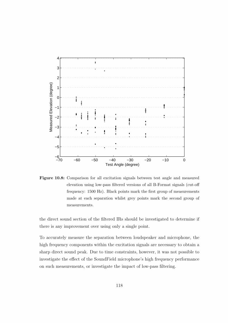
−70 −60 −50 −40 −30 −20 −10 0−6

−5

−4

−3

−2

−1

0

1

2

3

4

Test Angle (degree)

Mea

sure

d E

leva

tion

(deg

ree)

Figure 10.8: Comparison for all excitation signals between test angle and measured

elevation using low-pass filtered versions of all B-Format signals (cut-off

frequency: 1500 Hz). Black points mark the first group of measurements

made at each separation whilst grey points mark the second group of

measurements.

the direct sound section of the filtered IRs should be investigated to determine if

there is any improvement over using only a single point.

To accurately measure the separation between loudspeaker and microphone, the

high frequency components within the excitation signals are necessary to obtain a

sharp direct sound peak. Due to time constraints, however, it was not possible to

investigate the effect of the SoundField microphone’s high frequency performance

on such measurements, or investigate the impact of low-pass filtering.

118

Chapter 11

Multiple Microphone

Measurements

If the arrival time of a sound is measured at enough different points in space, it

is possible to determine the location of the original sound source. This chapter

describes different approaches that can be used dependant on the timing infor-

mation available and then gives an overview of the testing planned to investigate

their relative performance.

11.1 Theory

From the propagation delay measurements using a single omni-directional micro-

phone in chapter 9, it has been shown that the distance between a loudspeaker

and microphone can be measured to a sub-sample accuracy. From just this single

measurement the loudspeaker could be positioned anywhere on a sphere around

the microphone. By making a simultaneous measurement with a second micro-

phone, then a second sphere could be determined. If the distance between the two

microphones is know it is possible to calculate where these two spheres intersect,

thus reducing the possible set of loudspeaker positions to a circle. By using a third

119

microphone this can be reduced to a set of two points and a fourth microphone

can reduce this to a single point.

To ensure that a single point is found there are, however, certain limitations on the

arrangement of the microphones. For example, if all four microphones are posi-

tioned within a single plane then there is no way to determine which of two points,

one either side of the plane, is correct. Additionally, so far it has been assumed

that all distance measurements are exact. Although accuracy to the sub-sample

level means that the errors in distance are small, they do still exist and therefore

care must be taken to avoid amplifying them. The easiest method of reducing

the effect of these errors is to increase the separation between microphones—with

two microphones very close together even a small change in the value measured

by one would significantly change the position of the intersection between the two

spheres.

One implementation of this technique positions the four microphones on rectan-

gular axes: one at the origin and one on each axis equal distances, d, from the

origin[45]. In such a setup, it can be shown that the coordinates of the sound

source (x, y, z) are given by

x =(d2 + r2

o − r2x)

2d,

y =(d2 + r2

o − r2y)

2d,

z =(d2 + r2

o − r2z)

2d,

where ro, rx, ry and rz are the radii of the spheres around the microphones posi-

tioned at the origin and on the x, y and z axes respectively. This has the advantage

of greatly simplifying the process of determining the location of the loudspeaker

compared to some approaches, although it also has the potential to produce less

accurate results because it does not make full use of the available timing infor-

mation. One method that does utilise this extra timing information is a least

squares approach, minimising the differences between the measured and predicted

loudspeaker-microphone separations.

120

Instead of using the direct time-of-flight to calculate the loudspeaker position, the

differences in sound arrival time between the microphones can also be used. This

has the advantage of not needing to know exactly when the sound was transmitted

and so is far more suited to scenarios when the time delay through the complete

signal path is unknown to the required level of accuracy. From these differences in

time the differences in distance between the loudspeaker and each microphone can

be determined. With a single pair of microphones this results in a hyperboloid on

which the loudspeaker must be positioned. Through the use of more microphones,

the intersection of the different hyperboloids results in a single position for the

loudspeaker. The equations to determine the loudspeaker position from these

differences in distance are, however, highly non-linear and so to solve them many

different algorithms have been proposed[18].

An alternative arrangement of microphones that has been used is to place them

at the apexes of a regular tetrahedron. This is used by the Trinnov Optimizer to

determine the location of loudspeakers as well as measure the loudspeaker charac-

teristics and loudspeaker/room interaction[40]. The quoted precision of this system

is “better than 1 cm/2◦” when measuring the distance, azimuth and elevation of

loudspeakers, thus indicating that angle measurements using this microphone lay-

out are likely to be of similar accuracy to those achievable using a SoundField

microphone.

11.2 Planned Testing

Due to the need to revise the plan for this project, as described in chapter 14,

the time initially allocated to investigating the use of multiple microphones had

to be reallocated. For this reason no actual tests were implemented, although this

section will briefly describe the tests that were planned to be undertaken had time

allowed.

To enable a direct comparison between the use of multiple microphones and the

121

SoundField microphone, the initial tests were to be conducted using exactly the

same methodology as for the SoundField microphone, described in section 10.2.

Additionally a near identical wiring configuration to that shown in figure 10.2

would have been used, although using the sound desk instead of the dedicated

SoundField microphone control unit to amplify the four microphone signals.

Two different arrangements of the microphones were planned, testing both the

‘rectangular axes’ configuration and the regular tetrahedron. Following the tests

this would then allow the performance of different time of flight and time differ-

ence of arrival algorithms to be compared. However, the implementation of such

algorithms was expected to take a significant amount of time and so the algorithms

tested would have had to be chosen based on the time available.

122

Chapter 12

Ambisonics Decoding

For an Ambisonic system to be of any use, a method of generating the loudspeaker

feeds from the B-Format signals, as described in section 2.2, is required. Differ-

ent methods of achieving this have been proposed, although a common underlying

concept is to use virtual microphone responses, as described in appendix F, for mi-

crophones pointing directly at each of the loudspeakers. This can be implemented

using a ‘decoder matrix’, although the configuration of the virtual microphones to

generate this matrix differs between approaches.

To evaluate the performance of different decoding algorithms, the ‘Ambisonic equa-

tions’, which are a formal representation of certain “psychoacoustic criteria” as-

sociated with sound localisation, can be used[14]. Two different theories of sound

localisation to which these apply are the “Makita” theory, also known as the ‘ve-

locity vector’ theory, and the ‘energy vector’ theory. The first is more important

at low frequencies, where phase difference between the human ears is used to de-

termine a sound’s location, and provides a measure of the apparent direction of a

sound based on the gains of all the loudspeakers for a known virtual source loca-

tion. The second is more important at higher frequencies, where the “directional

behaviour of the energy field around the listener” is important, and also provides

a measure of the apparent direction of a sound source. The similarity in angle

123

between these two vectors indicates the ‘sharpness’ of a phantom image, whilst

the vector lengths indicate the stability of the sound location as the listener moves

their head[12, 14].

12.1 Decoder Types

The simplest form of decoder is that in which the directivity of all virtual mi-

crophones is the same, with no filtering applied to either the original B-Format

signals or the resulting loudspeaker feeds. The directivity used can then either be

determined by personal preference or optimised using the theories above. Extend-

ing this, shelving filters, with different gains for high and low frequencies, can be

applied to each of the B-Format signals prior to calculating the virtual microphone

responses[16]. This is equivalent to using two virtual microphones to calculate each

loudspeaker feed, with different directivities for high and low frequencies. Provided

the loudspeakers are placed in a regular array (all loudspeakers positioned evenly

on a circle around the listener), and the same directivities are used for all loud-

speakers then the apparent sound direction is the same as the encoded direction.

Furthermore, the perceived volume of a virtual sound source is the same regardless

of the direction of the source[42].

With irregular arrays, however, this approach cannot be used without result-

ing in excessive decoding artefacts[44]. A range of decoding schemes that have

been proposed include those for three or more “pairs of diametrically opposite

loudspeakers”[13] and those for “left/right symmetric” configurations with at least

two pairs of loudspeakers plus at least one further loudspeaker[14], similar to the

common 5 loudspeaker layout. Instead of using shelving filters, the last of these

used a “phase compensated band-splitting filter arrangement” to allow a com-

pletely different decoding matrix to be used at high and low frequencies, before

summing the outputs to generate each loudspeaker feed.

An alternative method of determining the required decoding parameters for similar

124

loudspeaker arrangements is given in [42, 44]. In these, a Tabu search (a memory

based heuristic search method) is used to optimise a set of ‘fitness’ equations

based on the velocity and energy vectors described above. Multiple potential sets

of decoding parameters are then produced, with subjective listening tests required

to determine the ‘best’ set. Although the implementation given is for the common

5 loudspeaker layout, “the methodology is applicable to any configuration”[44].

12.2 Decoder Implementation

Implementing a decoder for different loudspeaker arrangements can be divided

into two stages. Initially the decoding parameters for the particular arrangement

must be determined and then the B-Format signal must be decoded using these

parameters. In a completely automatic system, the first of these would have to take

the positional information for all of the loudspeakers, which could be anywhere in 3-

dimensional space, and produce an optimal set of decoding parameters. Although,

mathematically, the Tabu search algorithm in [42, 44] could be extended to cover

this far more generic case, this was beyond the scope of the project and so an

alternative was sought.

Investigation into other methods used to determine the decoding parameters for

irregular loudspeaker arrays found that certain assumptions about the loudspeaker

positions had always been made, such as left/right symmetry. Therefore, using

these methods when the assumptions were not met was expected to introduce

just as many decoding artefacts as using the methods for regular arrays when the

arrangement is not regular. So, a decoder for regular arrays was implemented

such that, provided the loudspeaker arrangement was close to being regular, a

completely functioning system could be implemented.

In this case, determining the decoding parameters from each loudspeakers position

requires minimal processing and so can be easily implemented alongside the B-

Format signal decoding. For a loudspeaker at azimuth, θ, and elevation, φ, its

125

feed can be calculated using the virtual microphone equation (F.4), where

rx = cos θ cosφ

ry = sin θ cosφ .

rz = sinφ

To implement different decoding for high and low frequencies either shelf filtering

with a single decoder or band-splitting with two decoders can be used. However,

provided the directivity, D, of the virtual microphone can be specified, the same

decoder block can be used in both instances. The resulting decoder block, written

for MATLAB, in which all loudspeaker feeds are generated simultaneously is shown

in listing 12.1.� �i f ( s ize (BFormatSig , 2)==3)

%Assume Z channel conta in s z e r o sspeakerFeeds = 0 .5 * ( BFormatSig ( : , 1 ) * sqrt (2 ) * (2− d i r e c t i v i t y ) . . .

+ BFormatSig ( : , 2 ) * ( d i r e c t i v i t y .* cos ( azimuth ) .* cos ( e l e v a t i o n ) ) . . .+ BFormatSig ( : , 3 ) * ( d i r e c t i v i t y .* sin ( azimuth ) .* cos ( e l e v a t i o n ) ) ) ;

elsespeakerFeeds = 0 .5 * ( BFormatSig ( : , 1 ) * sqrt (2 ) * (2− d i r e c t i v i t y ) . . .

+ BFormatSig ( : , 2 ) * ( d i r e c t i v i t y .* cos ( azimuth ) .* cos ( e l e v a t i o n ) ) . . .+ BFormatSig ( : , 3 ) * ( d i r e c t i v i t y .* sin ( azimuth ) .* cos ( e l e v a t i o n ) ) . . .+ BFormatSig ( : , 4 ) * ( d i r e c t i v i t y .* sin ( e l e v a t i o n ) ) ) ;

end� �Listing 12.1: Decoding of a B-Format signal, BFormatSig, for loudspeakers with the

specified azimuth and e l e v a t i o n . d i r e c t i v i t y is the directivity ofthe virtual microphone used to calculate the loudspeaker feed. Notethat multiple loudspeaker feeds can be calculated simultaneously ifd i r e c t i v i t y , azimuth and e l e v a t i o n are row vectors.

Although this could have then been used to create a frequency dependant decoder,

within the scope of the project this was not seen to be necessary and so instead a

method of implementing continuous decoding was investigated. Using the playrec

utility it had already been shown that continuous audio output was feasible from

within MATLAB. Additionally, because the decoder included no ‘memory’ of pre-

vious samples, it could be used to decode a signal in blocks rather than all in one

go. Therefore, the only remaining problem was obtaining the B-Format signal to

decode, to which two different solutions were found. The first was based around a

126

GUI in which the mouse could be dragged to change the position of a sound source.

In this case the mono sound source, S, was encoded into a B-Format signal, using

the equations

W =S√2

X = S cosα

Y = S sinα

Z = 0

where α is the azimuth of the virtual sound source. By encoding and then decoding

the signal in small blocks of samples (typically 512 samples long), the sound output

from the loudspeakers would move with only a small delay relative to the mouse

movement. However, it was found that if this latency was reduced too far, the audio

output would be stable the majority of the time although sporadically glitches

would occur due to other background tasks running on the computer.

An alternative source of B-Format signals were those available for download from

a range of websites1. Using these, combined with a version of the MATLAB

file wavread.m modified by Sylvain Choisel2 to support the WAVE-FORMAT-

EXTENSIBLE (WAVE EX) file format used by these files, it was possible to im-

plement a decoder that would, in theory, decode a file of any length. This was

achieved by reading a small block of samples from the file, decoding to the ap-

propriate loudspeaker feeds and then sending these samples to the playrec utility

before repeating the cycle. The two files used to implement this, playAmbiWav.m

and BFormatDec.m, as well as a file to encode a mono signal to a B-Format sig-

nal, and one to rotate, tilt and tumble a B-Format signal can all be found on the

accompanying CD, as described in appendix G.

1Sources of files include SoundField Ltd. (http://www.soundfield.com/downloads/

b-format.php), Angelo Farina’s public files (http://pcfarina.eng.unipr.it/Public/

B-format/), and the Ambisonic Bootlegs website (http://www.ambisonicbootlegs.net/). The

‘Composers’ Desktop Project’ Multi-Channel Toolkit provides useful command line tools to re-

format these files where necessary (http://www.bath.ac.uk/~masrwd/mctools.html).2wavexread.m available online at http://acoustics.aau.dk/~sc/matlab/wavex.html.

127

Chapter 13

Overall System Design

For an Ambisonics system to be easy to install and upgrade, one possibility is to

distribute the signal processing between a central unit and the loudspeakers using

wireless communications. However, for this to work effectively care must be taken

during the initial stages of the design. In this section the overall design of such a

system is considered, assuming the microphone(s) used for loudspeaker calibration

are attached to the central unit.

13.1 Signal Decoding

As a wireless surround sound system Ambisonics has the distinct advantage that

the loudspeaker feeds are all generated from the same B-Format signals. There-

fore, instead of transmitting each loudspeaker signal separately from the central

unit it should be possible to transmit the B-Format signals simultaneously to

all loudspeakers. By including loudspeaker specific decoding information within

the signal, each loudspeaker can then generate its own signal. This reduces the

amount of processing required in the central unit and also allows very simple sys-

tem expansion—the only real limit is the amount of time required to configure all

the loudspeakers with their own decoding parameters. Additionally, when only

128

using a first-order Ambisonic system, this reduces the total bandwidth required if

there are more than four loudspeakers.

Two further considerations are the latency through the system and the synchroni-

sation between the different loudspeakers. To achieve minimal latency, important

when the system is part of a larger multimedia setup, the buffering of data must be

kept to a minimum. If each loudspeaker could request retransmission of corrupted

data from the central unit, this could improve the quality of audio when used in

‘noisy’ RF environments. However, this requires enough data to be buffered to

allow the whole retransmission cycle to occur. Furthermore, if some data was cor-

rupted on arriving at one loudspeaker it may also have been corrupted at others,

thus meaning multiple loudspeakers may try and send re-transmission requests

simultaneously.

An alternative approach that would simplify both the loudspeakers and the central

unit would be to use a uni-directional link. This would allow for much smaller

buffers to be used but would increase the chance of the loudspeaker having either

no data or incorrect data to output. Using some form of error correction scheme

each loudspeaker would be able to correct for a limited number of received errors

and so reduce, although not eliminate, the effect of these. The ‘best’ compromise

between latency, resilience to errors and bandwidth required is one that can only

be made with knowledge of the equipment and intended environment.

Accurate synchronisation between the loudspeakers and the central unit is impor-

tant for two reasons: it ensures that the ‘same’ sound is not reproduced by one

loudspeaker before another, and it helps avoid either a buffer underrun or overrun

within the loudspeaker. The former does not impose a very strict requirement

provided any offset between loudspeakers in small and remains constant—this is

the same as an inaccuracy in the positioning of the loudspeaker. Inclusion of

timing information within the transmitted radio signal meets these requirements:

an internal clock within each loudspeaker would control the output of individual

samples whilst the timing information from the central unit would be used to fine

tune this clock on a regular basis.

129

To decode a B-Format signal, the decoding parameters must be based on the

location of the loudspeakers. Using the basic decoder implemented during the

project, the central unit would only need to tell each loudspeaker where it is posi-

tioned. However, to determine the optimum decoding parameters for an arbitrary

arrangement it is necessary to know where all loudspeakers are positioned. Imple-

menting this within the loudspeakers would therefore not be sensible because it

would rely on all the other loudspeakers calculating the same set of results. Thus

these calculations should be made by the central unit, which introduces a potential

problem: how to make this part of the system scalable. If bi-directional links were

used with each loudspeaker then a method of distributing this processing could

be implemented, although leaving the central unit processing for longer would be

another viable alternative, depending on how much longer it would actually take.

Using this approach a very basic decoding could be available almost immediately

with ‘better’ decodings becoming available over time. The system should not just

switch between these decodings, but they could be added to a list from which the

user can select.

13.2 Loudspeaker Location Detection

Assuming the use of uni-directional links, each loudspeaker would have to be given

a unique identifier. In the simplest system design the user would set these using

sequential numbers, telling the central unit how many loudspeakers exist. The

order of these numbers would not be important provided none were duplicated. An

alternative would be for each loudspeaker to be given its unique identifier during

manufacture. The central unit could then determine which loudspeakers were

present by using sound signals as a return link from the loudspeaker. Obviously if

bi-directional links are in use then this problem is greatly reduced.

As has been shown, the location of a loudspeaker can be determined when it pro-

duces a known excitation signal. By putting all loudspeakers into a ‘configuration’

mode it would be possible to send this signal using one of the audio channels within

130

the wireless link. Alternatively the excitation signal could be generated within the

loudspeaker and just triggered by the central unit. The former of these has two ad-

vantages: every loudspeaker does not have to be capable of generating the required

excitation signal, and the loudspeakers would be capable of working with different

central units, even if they use different algorithms to locate the loudspeakers.

No matter where the excitation signal is actually generated, the latency and syn-

chronisation between central unit and loudspeaker would have a significant impact,

under some techniques, on the possible accuracy of loudspeaker location. Using

a SoundField microphone, or equivalent intensity difference approach, then the

latency and synchronisation would impact the separation measurement but they

would not affect the angle measurement. In comparison, both angle and separation

measurements would be affected when using time-of-flight with four microphones

whilst neither would be affected when using time difference of arrival with four mi-

crophones. However, without testing all three of these methods it is not possible

to determine if this independence from latency and synchronisation is outweighed

by the technique being prone to larger errors.

13.3 Summary

It can be concluded that, theoretically, a system using a common uni-directional

link between a central unit and all loudspeakers could be implemented. Each

loudspeaker would need to be given a unique identifier and the central unit would

require a means of determining how many loudspeakers are present. Assuming

a first-order Ambisonics system, this link would need to carry four channels of

audio data at the required sample rate in addition to any data required for error

correction. Further to this a control data stream would be necessary including

information such as the decoding parameters and volume as well as the current

mode for each loudspeaker: calibration, mute or decoding. Should a loudspeaker

either temporally lose power or receive corrupted data, continuously repeating

this information in the control stream would then allow it to quickly resume as

131

required.

To calibrate the whole system the central unit would iterate through all loudspeak-

ers placing them into a calibration mode and then measuring their location using

one of the techniques previously discussed. With this information a very crude

decoding could be determined immediately, with better decodes produced over a

certain period of time, dependant on the number of loudspeakers, the algorithm

used and the processing power within the central unit. The resulting decoding

parameters would be sent to the loudspeakers and the Ambisonics system would

be functional.

Provided the necessary bandwidth to carry the extra data is available, this could

be expanded in different ways. For example a higher order Ambisonic system

could be implemented, requiring a larger number of audio data channels and more

decoding parameters to be determined, or loudspeaker frequency compensation

could be provided, requiring the central unit to tell each loudspeaker its required

compensation.

132

Chapter 14

Project Management

The large number of aims for this project meant that successful time management

was always going to be critical for the project to succeed. This chapter outlines

some of the decisions that were made during the project that affected what would

be achieved and by when.

An initial timetable was created which was believed to allow the project to be

completed on time. However, following the testing of different applications to find

one suitable for the project, as described in chapter 4, it was decided that the

playrec utility should be written to provide the required audio handling. Initially

the development of audio handling routines was planned to occur throughout the

project as necessary, but implementing this utility was seen to be beneficial to both

this and future projects and so the project timetable was revised. It was expected

that including the software development would mean not all of the aims of the

project could be achieved, so the different parts of the project were prioritised.

To generate a complete system implementation the utility was seen to be necessary

and so, combined with the advantages of using the same audio handling for the

duration of the project, this was given highest priority. Investigation into, and

implementation of, the different excitation signals was placed next because with-

out this no tests could be implemented. Following this the different microphone

133

tests and data analysis were seen to have similar priorities to the implementation

of a basic B-Format decoder. Although such Ambisonic decoders had been im-

plemented before, implementing it within MATLAB would help confirm correct

operation of the playrec utility, this being one of its target applications, as well as

show what could be achieved with the utility, opening up the opportunity for many

future projects. Because the different microphone tests would also have to occur

sequentially they were prioritised relative to each other. The first of these was

the separation measurements using a single microphone. Although this could have

been conducted directly as part of either of the other microphone configurations,

by initially implementing this on its own a test setup specifically for measuring

separation could be used and any problems with the excitation signals could be

eliminated before further tests. Next on the list was testing angle measurement

using the SoundField microphone. Its cost would probably prohibit its use in a

final commercial system, but it was decided that advantage must be taken of the

availability of this relatively rare and expensive piece of equipment. This resulted

in the tests using multiple microphones being given lowest priority.

The project timetable was re-created so that tasks would be completed in priority

order. However, to avoid unexpected problems preventing any further work some

items were still timetabled to occur simultaneously. At this stage all of the sets

of testing were still included, at the expense of removing the two spare weeks

previously allocated to allow parts of the project to overrun. Therefore, should

any problems arise it was possible that the project timetable would require further

updating.

Utility development and testing took longer than planned due to various problems,

such as the unexpected random addition of 5 output samples. Almost simultane-

ously, the implementation and testing of the creation and processing files for the

different excitation signals also took longer than expected. Therefore it was nec-

essary to revise the project timetable one last time. In this revision all tests using

multiple microphones were removed for two reasons: first, a long setup time was

expected for this configuration, accurately positioning all the microphones and

134

running preliminary tests; and second, allocating longer times for two sets of tests

rather than rushing three sets was deemed to be more beneficial for the project as

a whole. Even then it was found that far more time could have been spent on each

of the other sets of tests, such as analysing the effect of the room conditions or

loudspeaker orientation. This additional work had to be left until future projects

although that planned was completed according to the timetable.

135

Chapter 15

Further Work

The work undertaken during this project can be considered under four categories:

audio handling within MATLAB, loudspeaker location detection, Ambisonics de-

coding, and complete Ambisonic system implementation. There is more work that

could be done in each area, some of which is described in this chapter.

15.1 Audio Handling within MATLAB

The playrec utility, implemented to provide continuous audio input and output

within MATLAB, was designed to be versatile enough to support a wide range of

target situations, computers, soundcards and even operating systems. Therefore

further work based on the this utility could include:

� testing for correct functionality when using different computers and sound-

cards from those used during the initial development of the utility. By re-

peating the loop back tests described in section 7.5 the extent of the observed

unusual behaviour (the extra output samples) could then be determined.

� recompiling the utility to utilise an alternative soundcard interface or even to

136

operate on a different operating system, utilising the cross-platform support

offered by PortAudio.

� modifying the utility to utilise the additional functionality offered by

PortAudio V19.

� adding simultaneous support for multiple streams to allow more than one

soundcard to be used.

� writing MATLAB functions to determine the true extent of what can be

achieved using the utility such as the minimum latency that can be used

reliably, limits on the number of channels or sample rates (apart from those

inherent within PortAudio), or possible implementation of a real-time filter

or a spectrum analyser.

15.2 Loudspeaker Location Detection

The tests conducted to measure the accuracy with which the location of loud-

speakers can be determined included many assumptions. In a completely auto-

matic system, depending on the level of accuracy required, no assumptions can be

made and so further work should investigate the significance of these assumptions,

which included:

� the room being quiet and time-invariant;

� the speed of sound in the room remaining constant and hence the room’s tem-

perature, pressure, and even humidity and CO2 concentration not changing;

� the microphones, loudspeakers, amplifies, and D/A and A/D converters all

being identical to those used in the tests;

� the loudspeaker always being orientated to point directly at the microphone;

137

� the loudspeaker and microphone being positioned in the middle of the room,

ensuring the direct sound section of each IR could be easily distinguished

from room reflections.

� only one loudspeaker producing the excitation signal at any one time, some-

thing that should always be possible unless the user has wired two loud-

speakers to be fed with the same signal.

Analysing the results obtained when using a single microphone highlighted the

need for further work in the following areas:

� Peak sample detection. It was found that in some IRs the ripple either

side of the ‘peak’ sample had a larger magnitude than the peak itself. In a

final system it should not be assumed that the peak will always be positive

and therefore a method of correctly identifying the peak or reducing the

magnitude of the ripple should be investigated.

� Signal interpolation. After an investigation into different interpolation meth-

ods quadratic interpolation was used. However it was not determined if this

approach, when combined with the different IR measurement techniques,

provides a linear distribution of interpolated points between samples. There-

fore if very high levels of accuracy are required this should be practically

investigated using a test setup capable of making very accurate and small

movements of either a loudspeaker or microphone. Additionally a comparison

between quadratic interpolation and other techniques, such as oversampling,

could be made.

� Measurement accuracy. The grouping of the results at each test separation

indicated that the technique used to position the microphone was less accu-

rate than the accuracy of the measurements made with sound. Therefore the

same tests should be repeated in a much more strictly controlled environ-

ment so that any variations can be attributed to the measurement technique

and not the test methodology. As a part of this, a comparison between the

138

speed of sound determined from the room conditions and that predicted by

the results can be made. Furthermore this would enable a more accurate

comparison between the different excitation signals to be made—are some

more accurate than others when measuring distances, or were the discrepan-

cies observed due to other factors, such as slightly different acoustic centres

for different excitation signals.

� Multiple Acoustic Centres. Within a loudspeaker it is expected that its

acoustic centre is not in the same place at all frequencies. Therefore by

determining the location of the sound source using different ranges of fre-

quencies, it might be possible to determine not only the position but also

the orientation of the loudspeaker. However, this also introduces the extra

unknown of the maximum accuracy possible with only a limited range of

frequencies.

Using a SoundField microphone it was found that at high frequencies the B-Format

signals produced were significantly different from those expected. Therefore, as

described in section 10.3, by repeating these tests with another microphone of the

same model as well as different models of SoundField microphone the source of

this problem—calibration, the model of microphone, or SoundField microphones

in general—could be determined. Additionally the use of filtering, as preliminarily

tested, could be investigated further to find the optimum filter for measuring the

angle of the loudspeaker as well as that for measuring the separation. This could

also further the work presented by including variations in elevation as well as

azimuth.

To be able to compare the SoundField microphone approach to that using multiple

microphones, tests such as those described in section 11.2 could be conducted. Fur-

ther to these, the effect of inaccuracies in the relative positions of the microphones

could be investigated, relating this to the accuracies required during microphone

manufacture and therefore indirectly the overall cost of the system.

139

In addition to determining the actual location of the loudspeakers within a room,

further work could investigate how to measure other features of a particular Am-

bisonics setup, such as the apparent source location of early reflections and the

frequency response of the loudspeakers.

15.3 Ambisonics Decoding

When determining the decoding parameters for an Ambisonics decoder, such as

that implemented for the project, various assumptions about the loudspeaker lo-

cations are always made, such as left/right symmetry or equal distances from the

listener to all loudspeakers. In a system where the loudspeaker locations do not

fit these assumptions, using them to determine the decoding parameters could

introduce significant errors in the reproduced soundfield. Therefore a method of

determining the optimum decoding parameters for a completely arbitrary set of

loudspeaker locations should be investigated. For some sets of locations, such as

positioning all loudspeakers on one side of the listener, the results would obviously

be atrocious and so positioning the loudspeakers ‘sensibly’, which would need to

be defined, would always be required. However, even when including this there

would still be the need to determine the optimum value for many decoding pa-

rameters. For a system such as that proposed the investigation into this should

consider not only the performance of the resulting decoder but also the processing

power and time required to obtain it. The possibility of including frequency and

distance compensation within the decoder could also be considered.

15.4 Complete System Implementation

Although a top-level design for a complete system using wireless communica-

tion has been proposed, until some of the further work described above has been

completed such a system would be limited to using specific loudspeaker arrange-

140

ments. Therefore a practical implementation could be investigated further and

constructed, although if this were to happen the design should be very flexible to

allow changes to be made based on the results of other work. For example, until

the comparison between the different excitation signals and microphone arrange-

ments is completed the required processing within the central unit is unknown, as

is the impact of varying latency through the system. Additionally, until a suitable

method of calculating the decoding parameters has been determined, the required

resources to implement the algorithm efficiently is unknown.

141

Chapter 16

Conclusion

A suitable test system, based around a Personal Computer (PC), was designed. A

utility to be used within MATLAB was implemented and refined, allowing continu-

ous multi-channel audio input and output. This has been shown to be versatile: it

was used for all testing in determining the location of loudspeakers and also allowed

a continuous Ambisonics decoder to be implemented, running simultaneously with

a MATLAB GUI.

The accuracy to which microphone-loudspeaker separations can be measured using

sound was investigated with seven excitation signals based on Maximum Length

Sequences (MLS), Inverse Repeated Sequences (IRS), Optimum Aoshima’s Time-

Stretched Pulses (OATSP) and logarithmic sweeps. These were all found to mea-

sure propagation delays to a sub-sample level accuracy, with a strong indication

that the accuracy achievable is greater than that of the experimental method used.

The repeatability of the results using any one excitation signal was found to be very

good, with a maximum range of 0.039 of a sample interval across three readings.

Minor differences were observed between the different test signals, although these,

at under 0.10 of a sample interval, were also less significant than the inaccuracies

within the test procedure. The MLS and IRS excitation signals were found to be

more bearable than the other signals, although with this there was also a reduced

142

feeling of the ‘need’ to remain quiet, something which could favour the alternative

signals despite their poorer noise immunity. The accuracy of a room temperature

reading was found theoretically to have a significant impact on the accuracy with

which separation can be measured, although this was not tested.

Using a SoundField microphone and the same seven excitation signals it was found

that azimuth angle measurements could be accurate to within ±1◦. The B-Format

signals produced by the microphone deviated significantly from their theoretical

values at high frequencies, requiring low-pass filtering to obtain this level of accu-

racy. Additionally, the results indicated that the accuracy achievable was equal to,

or better than that of the test procedure. Due to time limitations, no tests could

be conducted to determine the accuracy achievable using four omni-directional

microphones.

An Ambisonics decoder was implemented within MATLAB based on virtual micro-

phones orientated towards each loudspeaker. This was shown to allow continuous

decoding of B-Format signals stored within a file as well as decoding B-Format

signals generated dynamically through controls on a MATLAB GUI.

A potential top-level design for a complete Ambisonic system using wireless com-

munications has been proposed. This system consisted of as many loudspeakers as

required and a central unit, into which the B-Format signals are fed and to which

the calibration microphone is attached. Sequentially the location of each loud-

speaker would be determined before converting this information into appropriate

decoding parameters and starting the decoding. Through implementing the decod-

ing within each loudspeaker, expansion of the system would be possible. However,

system expansion was seen to be a potential source of problems when calculat-

ing the decoding parameters—something which would most likely be implemented

solely in the central unit. Before the system can be fully implemented, further

work into the detection of loudspeaker positions and the calculation of decoding

parameters is required.

143

References

[1] N. Aoshima. Computer-generated pulse signal applied for sound measure-

ment. J. Acoust. Soc. Am., 69(5):1484–1488, May 1981.

[2] AV-JEFE, AV-LEADER Corporation. Lavalier mic page 2. http://www.

avleader.com.tw/lavalier-2.htm.

[3] A. J. Berkhout, D. de Vries, and P. Vogel. Acoustic control by wave field

synthesis. J. Acoust. Soc. Am., 93(5):2764–2778, May 1993.

[4] O. Cramer. The variation of the specific heat ratio and the speed of sound in

air with temperature, pressure, humidity and CO2 concentration. J. Acoust.

Soc. Am., 93(5):2510–2516, May 1993.

[5] K. de Boer. A remarkable phenomenon with stereophonic sound reproduction.

Philips Technical Review, 9(1):8–13, 1947.

[6] C. Dunn and M. O. Hawksford. Distortion immunity of mls-derived impulse

response measurements (abstract). J. Audio Eng. Soc., 41(5):314–335, May

1993.

[7] R. Elen. Ambisonics: The surround alternative. Surround 2001 Con-

ference, Dec. 2001. Available online at http://www.ambisonic.net/pdf/

ambidvd2001.pdf.

[8] A. Farina. Simultaneous measurement of impulse response and distortion with

a swept-sine technique. 108th Convention of the Audio Engineering Society,

Jan. 2000. Preprint 5093.

144

[9] A. Farina, R. Glasgal, E. Armelloni, and A. Torger. Ambiophonic principles

for the recording and reproduction of surround sound for music. 19th In-

ternational Conference of the Audio Engineering Society, June 2001. Paper

1875.

[10] A. Farina and F. Righini. Software implementation of an MLS analyzer with

tools for convolution, auralization and inverse filtering. 103rd Convention of

the Audio Engineering Society, Aug. 1997. Preprint 4605.

[11] A. Farina and E. Ugolotti. Software implementation of B-Format encoding

and decoding. 104th Convention of the Audio Engineering Society, Apr. 1998.

Preprint 4691.

[12] M. Gerzon. Multidirectional sound reproduction systems. United States

Patent Number 3,997,725, Dec. 14, 1976.

[13] M. Gerzon. Decoders for feeding irregular loudspeaker arrays. United States

Patent Number 4,414,430, Nov. 8, 1983.

[14] M. Gerzon and G. Barton. Surround sound apparatus. United States Patent

Number 5,757,927, May 26, 1998.

[15] M. A. Gerzon. Surround-sound psychoacoustics. Wireless World, Dec. 1974.

Reproduced online at http://www.audiosignal.co.uk/Surround%20sound%

20psychoacoustics.html.

[16] M. A. Gerzon. Ambisonics in multichannel broadcasting and video. J. Audio

Eng. Soc., 33(11):859–871, Nov. 1985.

[17] C. C. Gumas. A century old, the fast hadamard transform proves useful in dig-

ital communications. http://archive.chipcenter.com/dsp/DSP000517F1.

html.

[18] E. A. P. Habets and P. C. W. Sommen. Optimal microphone placement for

source localization using time delay estimation. Proc. of the 13th Annual

145

Workshop on Circuits, Systems and Signal Processing (ProRISC 2002), Veld-

hoven, Netherlands, pages 284–287, Nov. 2002. ISBN 90-73461-33-2.

[19] J. Hee. Impulse response measurements using MLS. http://home6.inet.

tele.dk/jhe/signalprocessing/mls.pdf.

[20] M. J. Leese. Ambisonic surround sound faq. Available online at http://

members.tripod.com/martin_leese/Ambisonic/faq_latest.html, 1998.

[21] D. G. Malham. Spatial hearing mechanisms and sound reproduction. Avail-

able online at http://www.york.ac.uk/inst/mustech/3d_audio/ambis2.

htm, 1998.

[22] D. G. Malham. Homogeneous and nonhomogeneous surround sound systems.

AES UK “Second Century of Audio” Conference, June 1999. An updated

version is available online at http://www.york.ac.uk/inst/mustech/3d_

audio/homogeneous.htm.

[23] S. Muller and P. Massarani. Transfer-function measurement with sweeps. J.

Audio Eng. Soc., 49(6):443–471, June 2001.

[24] R. Nicol and M. Emerit. Reproducing 3D-Sound for videoconferencing: a com-

parison between holophony and ambisonic. Proceedings of the First COST-G6

Workshop on Digital Audio Effects (DAFX98), Barcelona, pages 17–20, Nov.

1998. http://www.iua.upf.es/dafx98/.

[25] PortAudio. An Open-Source Cross-Platform Audio API. http://www.

portaudio.com/.

[26] PortAudio. Portaudio tutorial. http://www.portaudio.com/docs/pa_

tutorial.html.

[27] Pure Data (PD). About Pure Data. http://puredata.info/.

[28] B. Rafaely. Design of a second-order soundfield microphone (abstract). 118th

Convention of the Audio Engineering Society, May 2005. Preprint 6405.

146

[29] P. A. Ratliff. Properties of hearing related to quadraphonic reproduction.

Technical Report BBC RD 1974/38, BBC Research Department, Nov. 1974.

[30] V. C. Raykar, I. V. Kozintsev, and R. Lienhart. Position calibration of micro-

phones and loudspeakers in distributed computing platforms. IEEE Trans.

Speech Audio Process., 13(1):70–83, Jan. 2005.

[31] H. Robjohns. You are surrounded : Surround sound explained - part 1. Sound

on Sound, Aug. 2001. Reproduced online at http://www.soundonsound.com/

sos/Aug01/articles/surroundsound1.asp.

[32] P. Schillebeeckx, I. Paterson-Stephens, and B. Wiggins. Using mat-

lab/simulink as an implementation tool for multi-channel surround sound.

In Proceedings of the 19th International AES conference on Surround Sound,

pages 366–372, 2001.

[33] M. R. Schroeder. Integrated-impulse method measuring sound decay without

using impulses. J. Acoust. Soc. Am., 66(2):497–500, Aug. 1979.

[34] G.-B. Stan, J.-J. Embrechts, and D. Archambeau. Comparison of different

impulse response measurement techniques. J. Audio Eng. Soc., 50(4):249–262,

Apr. 2002.

[35] Steinberg Media Technologies GmbH. Our technologies. http://www.

steinberg.net/325_1.html.

[36] Y. Suzuki, F. Asano, H.-Y. Kim, and T. Sone. An optimum computer-

generated pulse signal suitable for the measurement of very long impulse

responses. J. Acoust. Soc. Am., 97(2):1119–1123, Feb. 1995.

[37] The MathWorks. Controlling Interruptibility (Creating Graphical User In-

terfaces, MATLAB Documentation). http://www.mathworks.com/access/

helpdesk_r13/help/techdoc/creating_guis/ch_pro15.html and within

the help documentation supplied with MATLAB.

147

[38] The MathWorks. mex (MATLAB Functions). http://www.mathworks.com/

access/helpdesk/help/techdoc/ref/mex.html and within the help docu-

mentation supplied with MATLAB.

[39] TransAudio Group. SoundField and B Format. http://www.soundfieldusa.

com/b_format.html.

[40] Trinnov Audio. Products. http://www.trinnov.com/products.php.

[41] J. Vanderkooy. Aspects of MLS measuring systems. J. Audio Eng. Soc.,

42(4):219–231, Apr. 1994.

[42] B. Wiggins. An investigation into the real-time manipulation and control

of three-dimensional sound fields. PhD thesis, University Of Derby, 2004.

Available online at http://sparg.derby.ac.uk/SPARG/PDFs/BWPhDThesis.

pdf.

[43] B. Wiggins. Multi-channel audio in simulink/matlab. Personal Communica-

tion via eMail, Feb. 10, 2006.

[44] B. Wiggins, I. Patterson-Stephens, V. Lowndes, and S. Berry. The design and

optimisation of surround sound decoders using heuristic methods. Proceedings

of UKSim 2003, Conference of the UK Simulation Society, pages 106–114.

Available online at http://sparg.derby.ac.uk/SPARG/PDFs/SPARG_UKSIM_

Paper.pdf.

[45] Y. Yamasaki and T. Itow. Measurement of spatial information in sound fields

by closely located four point microphone method. J. Acoust. Soc. Jpn. (E),

10(2):101–110, 1989.

148

Appendices

149

Appendix A

MEX-file Overview

MEX-files are shared libraries which can be executed from within MATLAB. They

can be compiled from C, C++, or Fortran source code using the mex function within

MATLAB [38], or alternatively they can be compiled using a separate compiler

creating a ‘dll’ file within Windows. For instructions on how to use Visual Studio

to achieve this see Appendix C.

Throughout this project only C was used to create MEX-files and so this overview

is based on using C, although many of the concepts are similar when using Fortran.

A.1 Entry Point Function

Within a C MEX-file there must be an entry point function called mexFunction.

This is executed by MATLAB whenever the library is used, achieved by typing

the name of the MEX-file in the same way as m-files can be used. No matter

how many variables are supplied to or expected from the MEX-function within

MATLAB, the entry point function always receives four parameters:

nlhs The number of variables expected to be returned.

150

plhs A pointer to an array of pointers of length nlhs, used to return the expected

number of variables.

nrhs The number of variables supplied to the MEX-function.

prhs A pointer to an array of length nrhs of pointers to the supplied variables.

All variables are transferred between the MEX-file and MATLAB using C

structures of type mxArray. A set of functions are then supplied to operate on

these mxArrays—creating, modifying and destroying them. Examples of such

functions include mxCreateStructMatrix ( ) , mxSetField ( ) , mxGetScalar ( ) and

mxDestroyArray ( ) . Additionally there are a set of functions used to determine

the type of variable stored within a mxArray, such as mxIsChar ( ) , mxIsComplex ( )

and mxIsStruct ( ) . Utilising these functions, the type of variables supplied as

parameters from within MATLAB can be determined, the required data can

be extracted from them and new variables can be created for use as return

parameters.

A.2 Memory management

With MEX-files, as with any applications written in C, correct memory man-

agement is very important. However, to achieve this the lifetime of dynamically

allocated memory must be taken into account:

� All mxArrays passed to the entry point function are managed by MATLAB

and must not be freed or modified within the MEX-file.

� All mxArrays created to be used as return parameters and added to plhs are

managed by MATLAB and are automatically freed once they are no longer

required.

151

� All other mxArrays are also freed by MATLAB when the entry point

function returns unless the mxArray has been marked as ‘persistent’ using

mexMakeArrayPersistent ( ) . In this case MATLAB will never free the

memory and instead it must be freed by the MEX-file once it is no longer

required.

� Memory allocation using the standard C functions, such as c a l l o c ( ) and

malloc ( ) , is not recommended and instead the ‘mx’ equivalents, such as

mxCalloc ( ) and mxMalloc ( ) , should be used where possible. Such memory

has the same lifetime as mxArrays and can, if required, be made persistent us-

ing mexMakeMemoryPersistent ( ) . In some scenarios, such as when including

source code that has already been written, the standard C functions might

need to be used. Any memory allocated in this way will never be freed by

MATLAB and so must always be freed once it is no longer required.

Once a MEX-file has been used, it remains loaded within MATLAB and so

all global variables and all persistent dynamically allocated memory remain

unchanged between uses of the MEX-file. To ensure all memory is freed after the

MEX-file has been used for the last time an exit function can be registered using

mexAtExit ( ) . Once registered, the function will be called by MATLAB before

the library is unloaded, such as when MATLAB is closed or the MATLAB c l e a r

command is used. The function must free all memory that has been dynamically

allocated and not freed either explicitly or automatically by MATLAB.

A.3 Textual Display

From within MEX-files it is possible to display text within the MATLAB command

window using similar commands to those used in m-files:

mexPrintf() This is very similar to the C function p r i n t f and the MATLAB

command f p r i n t f ( ) when f i d is omitted.

152

mexWarnMsgTxt() mexWarnMsgIdAndTxt() These display a warning al-

though do not terminate the MEX-file. They are similar to different versions

of the MATLAB command warning ( ) .

mexErrMsgTxt() mexErrMsgIdAndTxt() These display an error, terminate

the MEX-file and return control to the MATLAB prompt. They are similar

to different versions of the MATLAB command e r r o r ( ) .

A.4 Providing Help

Although text can be displayed within the command window when a MEX-file

is used, it cannot be used to display help information when the MATLAB help

command is used. Instead, a m-file with the same name as the MEX-file must be

created to contain the help information. This will not affect the operation of the

MEX-file and will only be used when help is requested.

More information on MEX-files can be found within the “External Interfaces” and

“External Interfaces Reference” sections of the MATLAB help1.

1Supplied with MATLAB and available online at http://www.mathworks.com/access/

helpdesk/help/techdoc/matlab.html

153

Appendix B

PortAudio Overview

PortAudio is a “free, cross platform, open-source, audio I/O library” written in C,

providing a “very simple API for recording and/or playing sound using a simple

callback function”[25]. For the duration of this project V18.1 was used because it

was the latest non-development versions available and it provided all the function-

ality required.

The library operates by calling a registered function with two buffers—one con-

taining recorded samples and the second to be populated with samples to play.

This callback function is automatically called by the library and so it cannot be

predicted when it will run, just that it will run regularly enough to avoid glitches

in audio. This assumes, of course, that the buffers have been configured correctly

and the function does not take too long to execute. For applications that only play

samples from a larger play buffer and record samples to a larger record buffer, such

an interface makes this a simple case of copying memory. Additionally, through

this type of interface ‘pausing’ the audio stream can be achieved by ignoring the

supplied record buffer and zeroing all values in the play buffer. Due to the buffer-

ing of recorded samples this approach effectively pauses recording slightly before

playing but then it also resumes recording before playing by the same amount.

However, in most applications this would not be problematic.

154

To configure the library to start using the callback, the following procedure must

be followed[26]:

1. Initialise PortAudio using P a I n i t i a l i z e ( ) .

2. Open a PortAudio Stream using either Pa OpenDefaultStream ( ) or

Pa OpenStream ( ) . This configures all the stream settings such as which

device, channels, sample rate and bit depth to use. Additionally it registers

the function to be used as the callback function described above.

3. Call Pa StartStream ( ) to start the library calling the callback and hence

start audio input and output. Once the stream has started this function

returns for the thread to continue.

When the library is no longer required, the following procedure must be

followed[26]:

1. Stop the stream by either returning 1 from the callback function or calling

Pa StopStream ( ) . The former always stops the callback from being called

although in some circumstances when using the latter the callback might be

called one more time, despite Pa StreamActive ( ) reporting the stream as

inactive. This was found to cause problems when stopping the stream and

then immediately freeing memory that the callback used. One solution is to

always use the callback to stop the stream, and then wait for the stream to

stop according to Pa StreamActive ( ) before freeing memory.

The stream can be started again using Pa StartStream ( ) .

2. Close the stream using Pa CloseStream ( ) . New streams can still be opened

as described above.

3. Terminate PortAudio using Pa Terminate ( ) . The library should not be used

once this has been called unless it has been initialised again.

155

If required multiple streams can run simultaneously using either the same or dif-

ferent callbacks. To identify which stream is calling the callback a pointer can be

supplied when opening the stream. This pointer can be of any type and is passed

to the callback.

Although the C code required to use PortAudio does not have to be changed to use

different operating systems or audio interfaces, the files used from the PortAudio

SDK do have to change. Additionally, when using the ASIO implementation a

SDK from the developers section of Steinberg’s website1 must be obtained.

For more information on the PortAudio functions refer to portaudio.h within the

PortAudio SDK2 and for configuration information see the PortAudio tutorial[26].

1http://www.steinberg.net/2Available online at http://www.portaudio.com/download.html

156

Appendix C

Configuring Visual Studio

This section provides configuration information to allow Microsoft Visual Studio

to create MEX-files that can use PortAudio. For a basic overview of MEX-files

and PortAudio see Appendices A and B respectively.

MEX-files can be compiled either within MATLAB or using a separate compiler.

The latter is initially more complicated to configure although once configured

it allows for easier development through the use of an Integrated Development

Environment (IDE), something especially useful when multiple files are being used.

Due to the need to include source code from the PortAudio SDK and the Steinberg

ASIO SDK, the latter approach was considered much more suitable. The available

IDE was Microsoft Visual Studio 2005 Professional Edition, which was configured

as follows1 to produce suitable MEX-files for use within MATLAB:

1. Install MATLAB and Visual Studio.

1Configuration is based on a combination of the pa wavplay utility source code (http://

sourceforge.net/projects/pa-wavplay/), the PortAudio tutorial (http://www.portaudio.

com/docs/), MATLAB documentation “Custom Building on Windows” (http://www.

mathworks.com/access/helpdesk/help/techdoc/matlab_external/f24571.html) and mod-

ifications found to be necessary throughout the course of the project.

157

2. Download and extract the PortAudio SDK2 and the Steinberg ASIO SDK3

to suitable locations. This configuration is based on PortAudio SDK V18.1

and Steinberg ASIO SDK 2.1.

3. Create a new Visual C++ Win32 Console Application, specifying an ‘Empty

project’ and ‘DLL’ application type.

4. Add to the project the files pa_common\pa_lib.c, pa_common\portaudio.h,

pa_common\pa_host.h and pa_asio\pa_asio.cpp from the PortAudio SDK

as well as host\asiodrivers.cpp, host\pc\asiolist.cpp and common\

asio.cpp from the ASIO SDK. None of these files should need modifying so

they can be used from their original location within the extracted SDKs.

5. Within the project properties:

� add additional compiler include directories: pa_common from the

PortAudio SDK; host, host\pc and common from the ASIO SDK; and

extern\include from the MATLAB installation directory.

� Change the character set to ‘Use Multi-Byte Character Set’ from the

default ‘Use Unicode Character Set’. This is to avoid compile errors

within asiolist.cpp.

� Add the C/C++ Preprocessor definitions MATLAB MEX FILE and WIN32

if not already included.

� Add linker dependencies: winmm.lib, libmex.lib, and libmx.lib.

Depending on which MATLAB functions are used some of these may

not be required.

� Add an additional linker library directory for the MATLAB .lib

files. Choose the most appropriate directory within extern\lib\ of

the MATLAB installation directory. Within MATLAB R14SP3

2Available online at http://www.portaudio.com/download.html3Available from the 3rd Party Developers section of Steinberg’s website at http://www.

steinberg.net/

158

there is no directory specifically for Visual Studio 2005 so

extern\lib\win32\microsoft\msvc71 should be used instead.

� Add the additional linker command line option / export : "mexFunction"

6. Add a new .c or .cpp file to the project to contain the entry point function

from MATLAB. Add the include statements� �#include "mex . h"#include " portaudio . h"� �

and the entry point function� �void mexFunction ( int nlhs , mxArray * plhs [ ] , int nrhs , const mxArray *prhs [ ] ){}� �

on which more information can be found in the MATLAB documentation4.

Following these steps the compiler should produce a file with the .dll extension.

To use the file within MATLAB either select the directory containing the file as the

‘Current Directory’ or add it to the MATLAB search path. On typing the name of

the file no warnings should be produced—if warnings or errors are produced they

should be rectified before continuing. To check the correct configuration of the

PortAudio SDK and the ASIO SDK, the code shown in listing C.1 can be used

instead of the file created in step 6 above.

A further advantage of using an IDE is the ease with which code can be debugged.

To start debugging, the ‘Local Windows Debugger’ option should be selected in

the Debugging section of the project properties and the path to the MATLAB

executable5 added as the ‘Command’. From within the IDE selecting ‘Start De-

bugging’ will then start MATLAB and the MEX-files can be debugged using all the

tools provided by Visual Studio. When starting debugging, a warning that no de-

bugging information could be found for MATLAB.exe may be displayed. Despite

this, debugging of the MEX-file can continue without problems.

4See “mexFunction (C)” within the help documentation supplied with MATLAB and online at

http://www.mathworks.com/access/helpdesk/help/techdoc/apiref/mexfunction_c.html.5\bin\win32\MATLAB.exe within the MATLAB installation folder

159

� �/* p a d l l t e s t . c*

* A s ing l e−f unc t i on f i l e to be used in con junct ion with the PortAudio SDK* to c r e a t e a MATLAB MEX− f i l e . Returns a s t r u c tu r e matrix conta in ing* i n fo rmat ion o f a l l a v a i l a b l e d ev i c e s . Although t h i s does not t e s t audio* throughput , i t can be used to t e s t f o r c o r r e c t compi l e r and l i n k e r* c on f i g u r a t i on .*

*/

#include "mex . h"#include " portaudio . h"

void mexFunction ( int nlhs , mxArray * plhs [ ] , int nrhs , const mxArray *prhs [ ] ){

const char * f i e l d names [ ] = {"deviceID " , "name" , " inputChans" , "outputChans" } ;const PaDeviceInfo *pdi ;int i ;PaError e r r ;

i f ( n lhs > 1) {mexErrMsgTxt ( "Too many output arguments expected " ) ;

}

e r r = P a I n i t i a l i z e ( ) ;i f ( e r r != paNoError ){

Pa Terminate ( ) ;mexPrintf ( "Error number : %d\nError message : %s \n" ,

e r r , Pa GetErrorText ( e r r ) ) ;mexErrMsgTxt ( "The above e r r o r occured when i n i t i a l i z i n g PortAudio" ) ;

}

plhs [ 0 ] = mxCreateStructMatrix (1 , Pa CountDevices ( ) ,s izeof ( f i e l d names ) / s izeof (char*) , f i e l d names ) ;

for ( i = 0 ; i < Pa CountDevices ( ) ; i++){

pdi = Pa GetDeviceInfo ( i ) ;

i f ( pdi != NULL){

mxSetField ( p lhs [ 0 ] , i , "deviceID " , mxCreateDoubleScalar ( i ) ) ;mxSetField ( p lhs [ 0 ] , i , "name" , mxCreateString ( pdi−>name) ) ;mxSetField ( p lhs [ 0 ] , i , " inputChans" ,

mxCreateDoubleScalar ( pdi−>maxInputChannels ) ) ;mxSetField ( p lhs [ 0 ] , i , "outputChans" ,

mxCreateDoubleScalar ( pdi−>maxOutputChannels ) ) ;}

}Pa Terminate ( ) ;

}� �Listing C.1: Sample test file which can be used to confirm correct configuration of

Visual Studio to produce MEX-files including ASIO Driver support.

160

Appendix D

playrec Utility Help Information

Within the p layrec utility an overview of the utility’s operation is provided by

the ‘about’ command, and help information for each of the commands is provided

through the ‘help’ command. This section reproduces all of this information di-

rectly as it is displayed by the utility within the MATLAB Command Window.

D.1 Utility overview

This playrec utility has been written to provide versatile access to soundcards

via Steinberg’s ASIO API. It is based on PortAudio, a free, open-source audio

I/O library, so should easily be portable to either WMME or DirectSound under

Windows, or even to different platforms just by recompiling with the relevant files.

A basic outline of how to use this utility is provided below. For more information

on any command type ‘help’ as the first parameter followed by the command of

interest as the second parameter.

All commands are accessed through the one function in MATLAB. This is achieved

by specifying the name of the command to run as the first parameter in the function

call followed by any additional parameters as required by the command. A list of

161

all available commands can be displayed by supplying no parameters when calling

the function.

Before any audio can be played or recorded, the utility must be initialised to use

the required sample rate and device(s). Initialisation can be achieved using the

‘init’ command, supplying the ID of the required audio device(s) as returned by

‘getDevices’. Once successfully initialised, the sample rate or device(s) to be used

cannot be changed without first resetting the utility using the ‘reset’ command.

This clears all previously recorded data so use it with care. To check if the utility

is currently initialised, use the ‘isInitialised’ command.

The utility divides time up into “pages”, with no restrictions on the duration of

any one page, although with very short pages skipping in the audio may occur.

Additionally there can be as many pages as required, provided the utility can

allocate memory to store all the pages. Pages are joined together sequentially in the

order they are added, with each page starting the sample after the previous page

finishes. The duration of a page is determined by the longest channel contained

within the page. Therefore if, for example, the record channels are 1000 samples

long whilst output channels are only 900 samples long, the page will be 1000

samples long and the final 100 output samples of the page will automatically be

set to 0.

When each page is added, the channels that are to be used for recording and/or

output are specified (depending on the command used to add the page). The chan-

nels used must be within the range specified during initialisation and no channel

can be duplicated within a channel list. Within these limits, the channel list for

each page can be different and each list can contain as many or as few channels as

required in any order. All output channels not provided with any data within a

page will output 0 for the duration of the page. Similarly, during any times when

there are no further pages to process 0 will be output on all channels.

Each page has a unique number which is returned by any of the commands used

to add pages (‘playrec’, ‘play’ or ‘rec’). When a page is added, the utility does not

162

wait until the page has completed before returning. Instead, the page is queued

up and the page number can then be used to check if the page has finished, using

‘isFinished’. Alternatively a blocking command, ‘block’, can be used to wait until

the page has finished. To reduce the amount of memory used, finished pages are

automatically condensed whenever any command is called in the utility. If a page

contains any recorded data, this is left untouched although any output data within

the page is removed. If the page does not contain any recorded data, the whole

page is deleted during this page condensing. For this reason if either ‘isFinished’,

‘block’ or ‘delPage’ indicate the page number is invalid this means the page either

never existed or has already finished and then been deleted during page condensing.

For pages containing recorded data, the data can be accessed using the ‘getRec’

command. This does not delete the data so it can be accessed as many times as

required. To delete the recorded data, the whole page must be deleted using the

‘delPage’ command. This command will delete pages no matter what their current

state: waiting to start, currently active or finished. If no page number is supplied,

all pages will be deleted, again regardless of their state.

To ascertain which pages are still left in memory, the ‘getPageList’ command can

be used, returning a list of the pages in chronological order. NOTE: there may

have been gaps of silence or other pages between consecutive pages in this list due

to pages either being automatically or explicitly deleted as detailed above. To

determine if there were gaps between pages due to all pages finishing processing

before new ones are added, the commands ‘getSkippedSampleCount’ and ‘reset-

SkippedSampleCount’ can be used.

The page that is currently being output is returned by ‘getCurrentPosition’, along

with an approximate sample position within the page. Additionally, the page num-

ber of the last completed page still resident in memory is returned by ‘getLastFin-

ishedPage’. NOTE: this might not be the most recent page to finish if that page

has been deleted either during page condensing (ie contained no recorded data) or

through the use of ‘delPage’.

163

Finally, the utility can be paused and resumed using the ‘pause’ command. This

will manipulate all output and recording channels simultaneously to ensure syn-

chronisation is always maintained. This command can also be used to ascertain if

the utility is currently running or paused.

D.2 Command specific help

D.2.1 help

[ ] = help (commandName)

Displays command specific usage instructions.

Input Parameters

commandName name of the command for which information is required

D.2.2 about

[ ] = about ( )

Displays information about this utility

D.2.3 getDevices

[ d e v i c eL i s t ] = getDev ice s ( )

Returns information on the available devices within the system, including ID,

name, and number of channels supported.

164

Output Parameters

deviceList Structure array containing the following fields for each device:

‘deviceID’ - ID used to refer to the device; ‘name’ - textual name of the

device; ‘inputChans’ - number of input channels supported; ‘outputChans’ -

number of output channels supported

D.2.4 init

[ ] = i n i t ( sampleRate , playDevice , recDevice , {playMaxChannel } ,

{ recMaxChannel } , { f ramesPerBuf fer })

Configures the utility for audio output and/or input based on the specified con-

figuration. If successful the chosen device(s) will be running in the background

waiting for the first pages to be received. If unsuccessful an error will be generated

containing an error number and description.

All channel numbers are assumed to start at 1. If the maximum channel number to

be used is not specified, the maximum number of channels that the device supports

is used. Specifying a maximum number of channels verifies the device supports the

required number of channels as well as potentially slightly reducing the utility’s

processor usage.

If an optional value is specified, all previous optional values must also be specified.

Input Parameters

sampleRate the sample rate at which both devices will operate

playDevice the ID of the device to be used for output (as returned by

‘getDevices’), or -1 for no device (ie output not required)

165

recDevice the ID of the device to be used for recording (as returned by

‘getDevices’), or -1 for no device (ie recording not required)

playMaxChannel (optional) a number greater than or equal to the maxi-

mum channel that will be used for output. This must be less than or equal

to the maximum number of output channels that the device supports. Value

ignored if playDevice is -1.

recMaxChannel (optional) a number greater than or equal to the maximum

channel that will be used for recording. This must be less than or equal

to the maximum number of input channels that the device supports. Value

ignored if recDevice is -1.

framesPerBuffer (optional) the number of samples to be processed in each

callback within the utility (ie the length of each block of samples sent by

the utility to the soundcard). The lower the value specified the shorter the

latency but also the greater the likelihood of glitches within the audio.

D.2.5 reset

[ ] = r e s e t ( )

Resets the system to its state prior to initialisation through the ‘init’ command.

This includes deleting all pages and stopping the connection to the selected au-

dio device(s). Generates an error if the utility is not already initialised - use

‘isInitialised’ to determine if the utility is initialised.

Use with care as there is no way to recover previously recorded data once this has

been called.

D.2.6 isInitialised

[ cu r r en tS ta t e ] = i s I n i t i a l i s e d ( )

166

Indicates if the system is currently initialised, and hence if ‘reset’ or ‘init’ can be

called without generating an error.

Output Parameters

currentState 1 if the utility is currently initialised, otherwise 0.

D.2.7 playrec

[ pageNumber ] = p layrec ( p layBuf fer , playChanList , recDuration ,

recChanList )

Adds a new page containing both sample input (recording) and output (playing).

Generates an error if the required memory cannot be allocated or if any other

problems are encountered.

The length of the page is equal to whichever is longer: the number of samples to

play or the number of samples to record.

Input Parameters

playBuffer a MxN matrix containing the samples to be played. M is the

number of samples and N is the number of channels of data.

playChanList a 1xN vector containing the channels on which the playBuffer

samples should be output. N is the number of channels of data, and should

be the same as playBuffer (a warning is generated if they are different but

the utility will still try and create the page). Can only contain each channel

number once, but the channel order is not important and does not need to

include all the channels the device supports (all unspecified channels will au-

tomatically output zeros). The maximum channel number cannot be greater

than that specified during initialisation.

167

recDuration the number of samples that should be recorded in this page, or

-1 to record the same number of samples as in playBuffer.

recChanList a row vector containing the channel numbers of all channels to

be recorded. Can only contain each channel number once, but the channel

order is not important and does not need to include all the channels the device

supports. This is the same as the order of channels returned by ‘getRec’.

The maximum channel number cannot be greater than that specified during

initialisation.

Output Parameters

pageNumber a unique number identifying the page that has been added - use

this with all other functions that query specific pages, such as ‘isFinished’.

D.2.8 play

[ pageNumber ] = play ( p layBuf fer , playChanList )

Adds a new page containing only sample output (playing). Generates an error if

the required memory cannot be allocated or if any other problems are encountered.

The page is the same length as that of playBuffer.

Input Parameters

playBuffer a MxN matrix containing the samples to be played. M is the

number of samples and N is the number of channels of data.

playChanList a 1xN vector containing the channels on which the playBuffer

samples should be output. N is the number of channels of data, and should

be the same as playBuffer (a warning is generated if they are different but

168

the utility will still try and create the page). Can only contain each channel

number once, but the channel order is not important and does not need to

include all the channels the device supports (all unspecified channels will au-

tomatically output zeros). The maximum channel number cannot be greater

than that specified during initialisation.

Output Parameters

pageNumber a unique number identifying the page that has been added - use

this with all other functions that query specific pages, such as ‘isFinished’.

D.2.9 rec

[ pageNumber ] = rec ( recDuration , recChanList )

Adds a new page containing only sample input (recording). Generates an error if

the required memory cannot be allocated or if any other problems are encountered.

The page is the same length as that specified by recDuration.

Input Parameters

recDuration the number of samples that should be recorded on each channel

specified in recChanList.

recChanList a row vector containing the channel numbers of all channels to

be recorded. Can only contain each channel number once, but the channel

order is not important and does not need to include all the channels the device

supports. This is the same as the order of channels returned by ‘getRec’.

The maximum channel number cannot be greater than that specified during

initialisation.

169

Output Parameters

pageNumber a unique number identifying the page that has been added - use

this with all other functions that query specific pages, such as ‘isFinished’.

D.2.10 pause

[ cu r r en tS ta t e ] = pause ({newPause })

Queries or updates the current pause state of the utility. If no parameter is sup-

plied then just returns the current pause status, otherwise returns the status after

applying the change to newPause.

Input Parameters

newPause (optional) the new state of the utility: 1 to pause or 0 to unpause

the stream. This can be either a scalar or logical value. If newState is the

same as the current state of the utility, no change occurs.

Output Parameters

currentState the state of the utility (including the update to newPause if

newPause is specified): 1 if the utility is paused or otherwise 0.

D.2.11 block

[ complet ionState ] = block ({pageNumber})

Waits for the specified page to finish or, if no pageNumber is supplied, waits until

all pages have finish. Note that the command returns immediately if the utility is

paused!

170

This uses very little processing power whilst waiting for the page to finish, although

as a result will not necessarily return as soon as the page specified finishes. For

a faster response to pages finishing use the ‘isFinished’ command in a tight while

loop within MATLAB, such as

while(playrec(‘isFinished’, pageNumber) == 0) end

This will run the processor at full power and will be very wasteful, but it does

reduce the delay between a page finishing and the MATLAB code continuing,

which is essential when trying to achieve very low latency.

Input Parameters

pageNumber (optional) the number of the page to wait until finished

Output Parameters

completionState 1 if either pageNumber is a valid page and has finished

being processed or pageNumber was not specified and all pages have finished

being processed. Note that page validity refers to when the function was

called and so now the page has finished it may no longer be a valid page.

0 if the stream is currently paused and neither return values of 1 or -1 apply.

-1 if the specified page is invalid or no longer exists. This includes pages that

have automatically been condensed, and hence have finished.

D.2.12 isFinished

[ complet ionState ] = i sF i n i s h ed ({pageNumber})

Indicates if the specified page is finished or, if no pageNumber is supplied, indicates

if all pages are finished.

171

Input Parameters

pageNumber (optional) the number of the page being tested

Output Parameters

completionState 1 if either pageNumber is a valid page that has finished

being processed or pageNumber was not specified and all pages have finished

being processed.

0 if either pageNumber is a valid page that has not finished being processed

or pageNumber was not specified and not all pages have finished being pro-

cessed.

-1 if the specified page is invalid or no longer exists. This includes pages that

have automatically been condensed, and hence have finished.

D.2.13 getRec

[ r e cBuf f e r , recChanList ] = getRec (pageNumber )

Returns all the recorded data available for the page identified by pageNumber. If

the page specified does not exist, was not specified to record any data, or has not

yet started to record any data then empty array(s) are returned. If the page is

currently being processed, only the recorded data currently available is returned.

Input Parameters

pageNumber used to identifying the page containing the required recorded

data

172

Output Parameters

recBuffer a MxN matrix where M is the number of samples that have been

recorded and N is the number of channels of data

recChanList a 1xN vector containing the channel numbers associated with

each channel in recBuffer. These channels are in the same order as that

specified when the page was added.

D.2.14 delPage

[ complet ionState ] = delPage ({pageNumber})

Deletes either the specified page or, if no pageNumber is supplied, deletes all pages.

Pages can be in any state when they are deleted - the do not have to be finished and

they can even be deleted part way through being processed without any problems

(in this case the utility will automatically continue with the next page in the page

list). If a problem is encountered whilst deleting a page

Input Parameters

pageNumber (optional) the number of the page to be deleted.

Output Parameters

completionState 0 if nothing is deleted (either there are no pages in the

page list or, if pageNumber was specified, no page with the specified number

exists), otherwise 1 is returned.

D.2.15 getCurrentPosition

[ currentPage , currentSample ] = getCurrentPos i t i on ( )

173

Returns the instantaneous current page number and sample number within this

page.

Output Parameters

currentPage the current page number, or -1 if either the utility is not ini-

tialised or no page is currently being processed (there are no pages in the list

or all pages are finished).

currentSample the current sample number within currentPage, or -1 if cur-

rentPage is also -1. This is only accurate to framesPerBuffer samples, as

returned by ‘getFramesPerBuffer’

D.2.16 getLastFinishedPage

[ l a s tPage ] = getLastFin ishedPage ( )

Returns the page number of the last finished page still resident in memory. Due

to automatic condensing/removal of pages that are no longer required, such as

those with just play data after they have finished, this may not be the most recent

page to have finished. Put another way, this returns the page number of the last

finished page in the pageList returned by ‘getPageList’.

Output Parameters

lastPage pageNumber of the most recently finished page still resident in

memory.

D.2.17 getPageList

[ pageLi s t ] = getPageLis t ( )

174

Returns a list of all the pages that are resident in memory. The list is ordered

chronologically from the earliest to latest addition.

Due to automatic condensing/removal of pages that are no longer required, such

as those with just play data after they have finished, this will not be a complete

list of all pages that have ever been used with the utility.

Output Parameters

pageList a 1xN vector containing the chronological list of pages, where N is

the number of pages resident in memory.

D.2.18 getFramesPerBuffer

[ f ramesPerBuf fer ] = getFramesPerBuffer ( )

Returns the number of frames (samples) that are processed by the callback inter-

nally within the utility (ie the length of each block of samples sent by the utility to

the soundcard). This is either the value specified when using ‘init’, or the default

value if the optional parameter was not specified in ‘init’.

Output Parameters

framesPerBuffer the number of frames returned by the utility internally

during each callback, or -1 if the utility is not initialised.

D.2.19 getSampleRate

[ sampleRate ] = getSampleRate ( )

Returns the sample rate that was specified when using ‘init’.

175

Output Parameters

sampleRate the current sample rate or -1 if the utility is not initialised.

D.2.20 getStreamStartTime

[ streamStartTime ] = getStreamStartTime ( )

Returns the unix time when the stream was started (number of seconds since the

standard epoch of 01/01/1970).

This is included so that when using the utility to run experiments it is possible to

determine which tests are conducted as part of the same stream, and so identify

if restarting the stream (and hence the soundcard in some scenarios) may have

caused variations in results.

Output Parameters

streamStartTime time at which the stream was started (in seconds since

the Epoch), or -1 if the utility is not initialised.

D.2.21 getPlayDevice

[ p layDevice ] = getPlayDevice ( )

Returns the deviceID (as returned by ‘getDevices’) for the currently selected out-

put device.

Output Parameters

playDevice the deviceID for the play device or -1 if no device was specified

during initialisation or the utility is not initialised.

176

D.2.22 getPlayMaxChannel

[ playMaxChannel ] = getPlayMaxChannel ( )

Returns the number of the maximum play channel that can currently be used.

This might be less than the number of channels that the device can support if a

lower limit was specified during initialisation.

Output Parameters

playMaxChannel the maximum play channel number that can currently be

used, or -1 if either no play device was specified during initialisation or the

utility is not initialised.

D.2.23 getRecDevice

[ r ecDev ice ] = getRecDevice ( )

Returns the deviceID (as returned by ‘getDevices’) for the currently selected input

device.

Output Parameters

recDevice the deviceID for the record device or -1 if no device was specified

during initialisation or the utility is not initialised.

D.2.24 getRecMaxChannel

[ recMaxChannel ] = getRecMaxChannel ( )

177

Returns the number of the maximum record channel that can currently be used.

This might be less than the number of channels that the device can support if a

lower limit was specified during initialisation.

Output Parameters

recMaxChannel the maximum record channel number that can currently be

used, or -1 if either no record device was specified during initialisation or the

utility is not initialised.

D.2.25 resetSkippedSampleCount

[ ] = resetSkippedSampleCount ( )

Resets the counter containing the number of samples that have been ‘missed’ due

to no new pages existing in the page list. See the help on ‘getSkippedSampleCount’

for more information.

D.2.26 getSkippedSampleCount

[ skippedSampleCount ] = getSkippedSampleCount ( )

Returns the counter containing the number of samples that have been ‘missed’ due

to no new pages existing in the page list. The term ‘missed’ is specifically referring

to the case where multiple consecutive pages are used to record a continuous

audio stream (and so input samples are missed), but is the same also for output

samples because the input and output samples within a page are always processed

simultaneously.

This value is incremented by one for every frame (ie one sample on every in-

put/output channel) of data communicated between the utility and soundcard

178

that occurred whilst there were no new pages in the page list. Using this it is

possible to determine, from within MATLAB, if any glitches in the audio have

occurred through not adding a new page to the page list before all other pages

have finished, such as in the case where the code within MATLAB is trying to

play/record a continuous stream.

Output Parameters

skippedSampleCount the number of samples, since last being reset, that

have occurred when there are no more pages in the pageList or -1 if the

utility is not initialised

179

Appendix E

Equipment List

Throughout this project the following equipment was used:

Personal Computer A Dual Pentium 4 2.8 GHz with 512 MB RAM running

Windows XP Professional SP2. A M-Audio Delta 1010LT soundcard (driver

version 5.10.00.0051) was used for all audio input and output with both

inputs and outputs set to “consumer” signal levels (-4dBu) with all bass

management turned off. Software used included MATLAB (version 7.1.0.246

R14 Service Pack 3) and Microsoft Visual Studio 2005 Professional Edition

(version 8.0.50727.42).

Amplifier A Marantz AV Surround Receiver SR4300, using the front and sur-

round channels through the direct signal 6.1 channel input connections. Vol-

ume set to -30dB during all tests.

Loudspeakers Audio Pro Focus SA-2 with grill removed and all distance mea-

surements made relative to the horizontal centre of the front of the cabinet.

Microphones

TCM110 Tiepin Microphone manufactured by AV-JEFE with the fol-

lowing quoted specification[2]:

180

Element Back electret-condenser

Polar Pattern Omni-directional

Frequency 50 Hz ∼ 18 kHz

Sensitivity -65 dB ±3 dB

CM4050 SoundField Microphone and Control Unit (serial number

615) manufacture by Calrec. Gain set to 40 dB, and all soundfield

manipulation disabled.

Microphone pre-amplifier For the TCM110 and one loop back signal an Allen

& Heath GL2000 was used. In both cases, both the channel equaliser and

high-pass filter were disabled, and the respective group faders were set to

+5 dB. The loop back channel used the line input and had +20 dB of gain

whilst the TCM110 channel used the microphone input with a gain of +60 dB

and a fader value between -5 dB and +5 dB dependant on the loudspeaker-

microphone separation.

181

Appendix F

B-Format Signal Manipulation

When the B-Format signals used to represent a soundfield at a single point in

space, as described in section 2.2, are summed together in different proportions

there are two important effects. The first of these allows the soundfield to be

rotated into any orientation required whilst the second allows virtual microphone

signals to be generated.

F.1 Soundfield Rotation

By summing together the first-order spherical harmonic components (X, Y and

Z) in different proportions it is possible to rotate, twist and tumble a recorded

soundfield such that it can be given any orientation within space[21]. This occurs

because the summing of weighted figure-of-8 polar patterns results in a single

figure-of-8 pattern with a different orientation, as shown in figures F.1 and F.2.

These both show rotation within a plane, although through the use of all three

first-order components 3-dimensional positioning of the figure-of-8 polar pattern

can be achieved. Thus, by creating three new orthogonal signals (X ′, Y ′ and Z ′)

a new B-Format signal can be created with the front pointing in any direction

compared to that of the original.

182

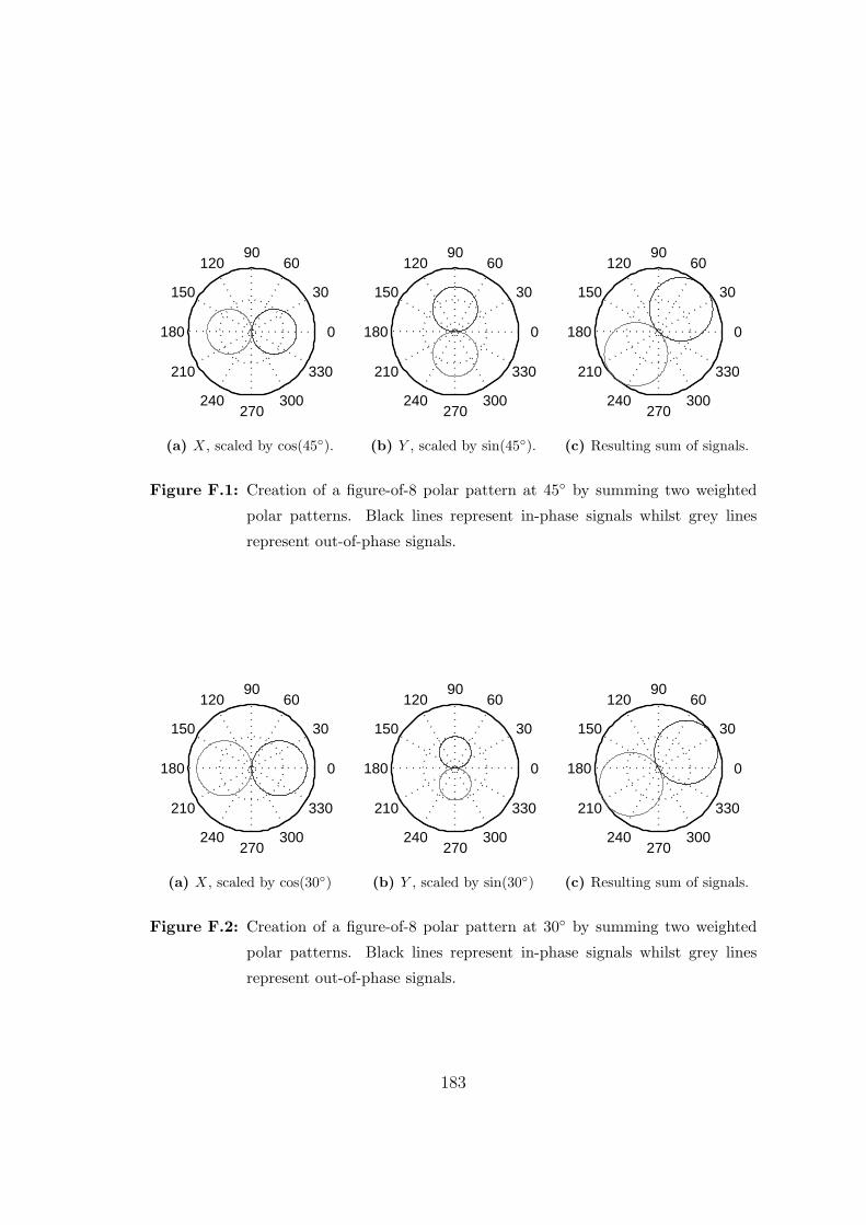
30

210

60

240

90

270

120

300

150

330

180 0

(a) X, scaled by cos(45◦).

30

210

60

240

90

270

120

300

150

330

180 0

(b) Y , scaled by sin(45◦).

30

210

60

240

90

270

120

300

150

330

180 0

(c) Resulting sum of signals.

Figure F.1: Creation of a figure-of-8 polar pattern at 45◦ by summing two weighted

polar patterns. Black lines represent in-phase signals whilst grey lines

represent out-of-phase signals.

30

210

60

240

90

270

120

300

150

330

180 0

(a) X, scaled by cos(30◦)

30

210

60

240

90

270

120

300

150

330

180 0

(b) Y , scaled by sin(30◦)

30

210

60

240

90

270

120

300

150

330

180 0

(c) Resulting sum of signals.

Figure F.2: Creation of a figure-of-8 polar pattern at 30◦ by summing two weighted

polar patterns. Black lines represent in-phase signals whilst grey lines

represent out-of-phase signals.

183

Rotating the soundfield about the Z-axis by θ is achieved usingX ′

Y ′

Z ′

=

cos θ − sin θ 0

sin θ cos θ 0

0 0 1

X

Y

Z

. (F.1)

Similarly, tilting by φ about the x-axis is given byX ′

Y ′

Z ′

=

1 0 0

0 cosφ − sinφ

0 sinφ cosφ

X

Y

Z

, (F.2)

and tumbling by ψ about the y-axis byX ′

Y ′

Z ′

=

cosψ 0 − sinψ

0 1 0

sinψ 0 cosψ

X

Y

Z

. (F.3)

Therefore, to implement rotation about the z-axis followed by tilting about the

x-axis, these operations can simply be implemented sequentially, givingX ′

Y ′

Z ′

=

1 0 0

0 cosφ − sinφ

0 sinφ cosφ

cos θ − sin θ 0

sin θ cos θ 0

0 0 1

X

Y

Z

.

F.2 Virtual Microphones

An alternative to summing only the first-order spherical harmonics is to include

the zeroth-order spherical harmonic (W ). This not only allows the orientation of

the resulting signal to be changed, but also the polar pattern—ranging from that

of an omni-directional microphone (only includes the W signal) to a figure-of-8

microphone (not including the W signal). This is controlled by the directivity

factor D in

V (~r) =1

2

[√2(2−D)W +D (rxX + ryY + rzZ)

](F.4)

184

where ~r is a unitary vector pointing in the direction of the required virtual mi-

crophone pattern, V (~r) [9]. (Note that the√

2 factor is included as the B-Format

standard includes a 3 dB reduction in W compared to X, Y , and Z.) D can take

any value in the range 0 to 2, with 0.5 producing a sub-cardioid polar pattern

(see figure F.3), 1.0 producing a cardioid polar pattern (see figure F.4) and 1.5

producing a hyper-cardioid polar pattern (see figure F.5).

30

210

60

240

90

270

120

300

150

330

180 0

(a) W , scaled by 0.75.

30

210

60

240

90

270

120

300

150

330

180 0

(b) X, scaled by 0.25.

30

210

60

240

90

270

120

300

150

330

180 0

(c) Resulting sum of signals.

Figure F.3: Creation of a virtual sub-cardioid microphone polar pattern using a direc-

tivity, D, of 0.5. Black lines represent in-phase signals whilst grey lines

represent out-of-phase signals.

185

30

210

60

240

90

270

120

300

150

330

180 0

(a) W , scaled by 0.5.

30

210

60

240

90

270

120

300

150

330

180 0

(b) X, scaled by 0.5.

30

210

60

240

90

270

120

300

150

330

180 0

(c) Resulting sum of signals.

Figure F.4: Creation of a virtual cardioid microphone polar pattern using a directivity,

D, of 1.0. Black lines represent in-phase signals whilst grey lines represent

out-of-phase signals.

30

210

60

240

90

270

120

300

150

330

180 0

(a) W , scaled by 0.25.

30

210

60

240

90

270

120

300

150

330

180 0

(b) X, scaled by 0.75.

30

210

60

240

90

270

120

300

150

330

180 0

(c) Resulting sum of signals.

Figure F.5: Creation of a virtual hyper-cardioid microphone polar pattern using a

directivity, D, of 1.5. Black lines represent in-phase signals whilst grey

lines represent out-of-phase signals.

186

Appendix G

CD Contents

The CD accompanying this project contains three folders: Documentation,

MATLAB_code and playrec_utility.

G.1 Documentation

This folder contains an electronic copy of this report and a copy of the initial

report submitted in February 2006.

G.2 MATLAB code

This folder contains the final MATLAB code used during the project. It is divided

into the following subfolders:

BFormatProcessing contains files to manipulate B-Format signals including cre-

ating them from a mono source, rotating, tilting and tumbling them, and

decoding them to generate loudspeaker feeds. This also contains a GUI

187

to demonstrate decoding using an encoded mono source, and a file to al-

low WAVE-FORMAT-EXTENSIBLE files containing B-Format signals to

be decoded in a block-wise manner.

CoreFunctions contains core files that were used throughout the project under

different circumstances. Many of these are ‘helper’ files that were used to

aid figure plotting. Other files include one to window a signal and another

to return the index of specific values (needles) within an array (haystack).

Files to implement linear and circular correlation and convolution are also

included, allowing other files to operate without the need for the Signal

Processing Toolbox.

IR ExcitationSignals contains all files required to create and process the four

different excitation signals used: MLS, IRS, OATSP and logarithmic sweep.

IR PeakDetection contains files used to detect the position and value of peaks

within an Impulse Response, using either peak sample, quadratic interpola-

tion or cubic interpolation. A file to trim an IR around its peak, including

support for multi-channel IRs, is also included.

PresentationGUIs contains GUIs used during a presentation given at the De-

partment of Speech, Music and Hearing (TMH), at the Royal Institute of

Technology (KTH), Stockholm on 23 May 2006.

Test and Analysis contains all files used to manage and manipulate the data

associated with all tests conducted.

UsefulFiles contains the file wavexread.m created by Sylvain Choisel and based

on the MATLAB file wavread.m. This file is used when playing WAVE-

FORMAT-EXTENSIBLE files containing B-Format signals and is also avail-

able online at http://acoustics.aau.dk/~sc/matlab/wavex.html.

Some of the files included are dependant on files contained in other subfolders.

188

G.3 playrec utility

This folder contains all of the source code used to compile the playrec utility. A

sample Microsoft Visual Studio Solution containing two projects is also included.

The first project is for the playrec utility whilst the second is for the test file shown

in listing C.1. This folder is divided into the following subfolders:

asiosdk2 For the sample Visual Studio Projects to compile the Steinberg ASIO

SDK must be downloaded and extracted to this folder. The SDK can be

downloaded from the 3rd Party Developers section of the Steinberg website

(http://www.steinberg.net/).

pa ASIO dll contains the sample Visual Studio Solution and three subfolders:

playrec containing the utility specific source code in the four files

mex_dll_core.c, mex_dll_core.h, pa_dll_playrec.c and

pa_dll_playrec.h;

release containing the files generated from compiling both the utility and

the test project, including the .dll files used by MATLAB;

testProject containing the test project source code in pa_dll_test.c.

To use the .dll files in the release folder within MATLAB either add

the folder’s path to the path list or set it as the current directory. The

playrec utility can then be used by typing p layrec at the MATLAB com-

mand prompt whilst the test project can be used by typing t e s tP r o j e c t .

portaudio v18 1 contains the PortAudio SDK V18 1 as downloaded from their

website (http://www.portaudio.com/download.html). This is required to

compile either of the included projects.

189