Camp & Maths. wrrh A&s. Primed I” Great Bnw.m.

Vol. II No 6. PP 6X-64 I. I985 wJ7-494318.5 163.00+ .oo 8 IYX5 Pergamon Press Ltd

AUTOMATIC INDEXED CALCULATION OF WACHSPRESS’ RATIONAL FINITE ELEMENT FUNCTIONS

G. R. DALTON Department of Nuclear Engineering Sciences, University of Florida, Gainesville, FL, U.S.A.

(Received July 1984)

Communicated by E. L. Wachspress

Abstract-A numerical method of calculating all of the polynomial coefficients for Wachspress’ rational finite element functions is presented. It requires only linear algebraic computations of matrix algebra and avoids the complicated constructions of geometric algebra used in the development of the rational

elements.

1. INTRODUCTION

The rapid increase in the use of irregularly shaped finite elements has emphasized the inadequacy of simple polynomials to serve as basis functions to fit, interpolate, differentiate and integrate a function specified at various vertices, points on sides, and points interior to the elements. It is now becoming clear that higher-order approximations to functions over finite elements have the capacity to improve not only the appearance, but also the convergence properties of the approximations[ 11. Recent numerical applications of higher-order approximations give specific examples of these improvements[2]. Recently, a new set of basis functions was presented by Wachspress[3]. The functions are ratios of polynomials which fit specified nodal values, and attain a prescribed degree of approximation over each element and its boundaries. Adjacent elements have the same polynomial variation along common edges, so that global continuity is assured. The continuous, analytic basis functions are amenable to interpolation, differentiation and integration. They are available for elements from triangles through N-sided polygons and their generalization, elements having sides which are algebraic curves. Any desire degree of approximation may be achieved in two-, three- and even higher-dimensional space.

Due to the manner in which these rational basis or wedge functions have been deduced from deep theorems of classical algebraic geometry, their construction tends to be heavily dependent on algebraic solutions to geometric problems. One may construct a unit wedge function for each node before one constructs the function that fits specified nodal values and has a prescribed degree of variation along the edges and over the element. This is essential for finite element application where nodal values are free parameters in a variational or Galarkin formulation. However, this is not essential for patchwork interpolation of data.

An alternate construction of both the basis wedges and composite fitting functions that depends only on the indexed computations of linear algebra is presented here. These matrix computations are implemented using a digital computer and require no geometric constructions whatsoever. Furthermore, the computation can be used to construct the general wedge basis functions of Wachspress as well as more general fitting functions over the element.

In Sec. 2, a few results from the theory of wedge construction will be described from the geometric point of view. It will be shown that a general interpolant over the element, represented as a linear combination of wedge functions times node values, has an alternate and useful linear- coefficient-polynomial-form that can be treated with the methods of conventional matrix algebra. In Sec. 3, a method for using linear algebra to solve for all of the unknown coefficients in the general function expression will be developed. This will be done in terms of specific polynomial fitting functions for the triangle, quadrilateral, etc. In Sec. 4 the theory for computation of the coefficients for up to degree-two fitting over polygons will be developed. In Sec. 5, comparisons with independent evaluations of several examples of basis functions will be presented and some of the computational difficulties encountered in the applications of the method introduced here will be presented. In Sec. 6, possible extensions of the method to elements with curved sides and to elements in three dimensions will be presented.

625

626 G. R. DALTON

2. GEOMETRIC BACKGROUND

On reading the discussion of Wachspress[3]. one observes that a rational function which

is linear on all the edges and has zero value on all but one vertex of a convex polygon can be constructed. Given a polygon with N sides as seen in Fig. 1, one first proposes the degree-one wedge function for node i as the ratio of two polynomials:

w,tx, y) = p,-,(.r, ~)iQ,~_~(x, y), (2.1)

where the subscripts N- 2 and N - 3 indicate the maximal degrees of the polynomials P(x, y) and Q(x, y). In particular, Q,_,(x, y) is a polynomial which vanishes on a curve of maximal degree-(N - 3). For example, for N = 5, one has

QN_3(x, y) = b. + b,x + bzy + 63x2 + b,y2 + bsxy. (2.2)

In fact, the coefficients bi can be determined by the requirement that the curve Q,._&, y) = 0

pass through all of the external intersection points (EIP’s), of the polygon (see Fig. 1). The polynomial PN_*(x, y) is the product of the N - 2, order-one forms which vanish on the N - 2 polygon edges that do not contain point i. Note that the leading b. term will be 1 except for the case where an EIP is located at the origin of coordinates, in which case b, must be 0.

If one defines the degree-one form for a line 1, 2 as

x y 1

Mx7 Y) = w,.,> = XI Yl 1 (2.3) x2 y, 1

then

PN-*(x9 Y) = tL+I.,c2) ... (Lv.I)t~I.‘) ... G-2.,-,). (2.4)

For the five-sided polygon (or 5-gon), N - 2 = 3, one has

pN_2(x, y) = aI + a2x + sjy + &x2 + a5y2 + a6xy

+ 8,X3 + a*y3 + agx2y + a,“q2.

It will also be of use to note the form, but not the details of the wedge for the ith node when the function is to be of degree two along each side as specified by the value of the function at an edge point as well as the comers. The function Q,,,_,(x, y) is the same for any degree of approximation. For the case of degree-two approximation over the N-sided polygon, the degree of P is N - 1. Thus for degree-two fitting one has

W,tx, Y) = h-,(x, y)lQ,v-4x3 ?I). (2.5)

Fig. I. A general N-sided polygon

Wachspress’ rational finite element functions 627

It is tempting to assume that P,_,(x, y) might be made up of products of quadric surfaces passing through the points on the nonadjacent sides. This is unfortunately not the case. However, the lack of such a simple extension causes no hardship. For degree-R approximation over the polygon one has

Wik Y) = PN+-R-2(x, yVQ,-3(x, y). (2.6)

In order to be specific one can consider the degree-l wedge for the triangle in Fig. 2. The basis function for point 1 is

W,(x, Y) = PI@, Y)Qo(x,, Y,)

Qok yV’,(x,, Y,)

L2.3k Y)

= L2.3(x,. YI)

x Y 1 xl Yl 1 = x2 Yl 1

I

x2 Yl 1. (2.7)

x3 Yl 1 x3 Yl 1

The divisor has been chosen to normalize the wedge W,(x, y) to unity at the point (xl, y,). For the convex quadrilateral (Fig. 3) the general degree-one wedge will have the form

WI& Y) =

=

f’2k Y) QI<XI, YI)

Qlk Y) P2(x,, YI)

a, + u2x + a3y + L&X2 + a5y2 + a,Xy (without normalization)

(2.8)

b,, + b,x + b2y

For the degree-one pentagon one has

P3(x, y) W;(x, y) = - =

a, + *** u,Xy + -a* a,,_$

Qz(x, Y) b,, + blx + b,y + --a bgy’ (2.9)

The number of terms in the general degree-N polynomial in x and y, such as P,,,(x, y) and Qdx, Y) is

Dim P,(x, y) is = (N + l)(N + 2)/Z!. (2.10)

If the polynomial has three independent variables (x, y, z) then

Dim PN(x, y, z) = (N + l)(N + 2)(/V + 3)/3!. (2.11)

One will find it useful to generalize the concept of the matrix operator of powers to treat polynomial systems of degree-N with K degrees of freedom, or dimensions. This matrix will give all of the powers of each independent variable in the degree-N polynomial in K dimensions.

3

Fig. 2. A triangle with degree-one variation.

628 G. R. DALTON

2

Fig. 3. A convex quadrilateral.

The rows will contain all monomials of degree m in K variables, where m runs from 1 to N. See Table 1 for examples of this matrix [P, N, K]. In addition one will need to define the matrices Q, R and S:

[Q, N, Kl = if’, N, Kl (2.12)

with the leading row of zeros omitted,

[R, N, K + l] = [P, N, K] (2.13)

with an additional column of zeros added at the right,

[S, N, K + 11 = [Q, N, Kl (2.14)

with an additional column of ones added at the right.

Note that whenever any of the matrices P, Q, R or S occur before another matrix as in

[P, N, KI[Cl (2.15)

it will be understood to mean

if’, NT Kl k=y,K [Cl, (2.16)

where the 7~~=,,~ indicates that the N tuples of powers in each row of the [P, N, K] matrix

operate on the N tuples of the coordinates in the columns of the [C] matrix to form the product of powers of coordinates in the terms in the polynomial P,,Jx, y, ... K).

One is now able to write Eq. (2.9) for the rational wedge for the 5-gon, using the [P] and

[Q] matrices as

ia, a2

W(x y) = (2.17)

1 + [h bz ... b,l[Q, 2,

Wachspress points out that a general function over the polygon can be constructed based on the wedge functions for each node times the values of the dependent variable z at each node. This will take the form

z(x, y) = {sum for i over all nodes} of z(x,, yi)W,(x, y) (2.18)

provided that each wedge is normalized to 1 at its node point. Then, the denominator Q is the same for all wedges and the general function z(x, y) is

~0, Y) = P.w+R-b, y)lQ,v-,k y). (2.19)

Wachspress’ rational finite element functions 629

The coefficients of Q are determined by the requirement that the curve Q(x, y) pass through the EIP’s of the element.

3. DEGREE-ONE ALGEBRAIC THEORY

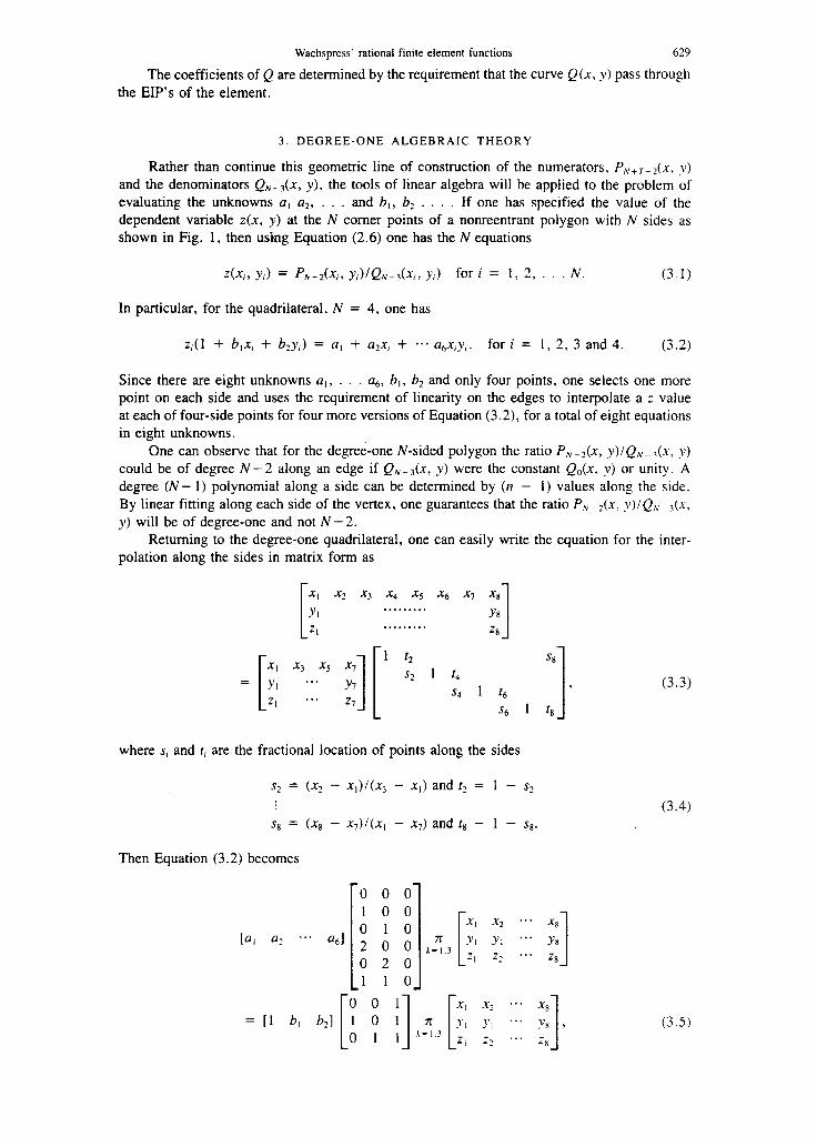
Rather than continue this geometric line of construction of the numerators, PN+T-Z(~, y) and the denominators Q,_,(x, y), the tools of linear algebra will be applied to the problem of evaluating the unknowns u, a2, . . , and b,, b2 . . . . If one has specified the value of the

dependent variable z(x, y) at the N comer points of a nonreentrant polygon with N sides as

shown in Fig. 1, then using Equation (2.6) one has the N equations

4x;, YJ = PN-2(x,, yi)IQN_3(Xi, yi) for i = 1, 2, . . N. (3.1)

In particular, for the quadrilateral, N = 4, one has

z;(l + b,x; + bzy,) = a, + a2x, + -** a,x,y,. for i = 1, 2, 3 and 4. (3.2)

Since there are eight unknowns a,, . . . u6, b,, b, and only four points, one selects one more

point on each side and uses the requirement of linearity on the edges to interpolate a z value at each of four-side points for four more versions of Equation (3.2), for a total of eight equations in eight unknowns.

One can observe that for the degree-one N-sided polygon the ratio PN-2(x, y)IQ~_~(x, y) could be of degree N - 2 along an edge if QN-Jx, y) were the constant QJx, y) or unity. A degree (N - 1) polynomial along a side can be determined by (n - 1) values along the side. By linear fitting along each side of the vertex, one guarantees that the ratio P,_ ?(x, y)/Q,+ 3(x. y) will be of degree-one and not N - 2.

Returning to the degree-one quadrilateral, one can easily write the equation for the inter- polation along the sides in matrix form as

XI x2 x3 x4 x5 x6 x7 x8

Yl . . . . . . . . . Yll 21 . . . . . . . . . Z8 1

XI x3 x5 x7

= YI -.- Y7 [ l[ 1 12 %

s2 1 t4

s4 1 t6 1 7 z, ... z7 s6 1 h

(3.3)

where si and ti are the fractional location of points along the sides

s2 = (x2 - x,)/(x3 - x,) and tz = 1 - s?

(3.4) sfj = (X8 - x7)/(x, - x7) and ts - 1 - s8.

Then Equation (3.2) becomes

(3.5)

630 G. R. DALTON

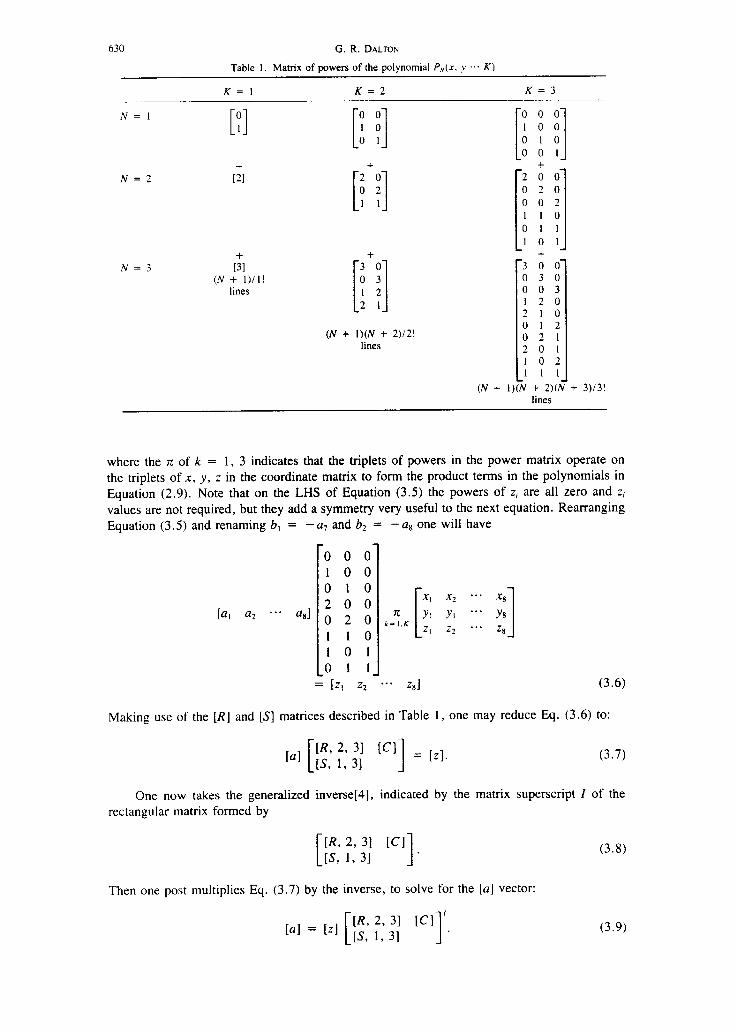
Table 1. Matrix of powers of the polynomial f,,(x, .v ... K)

K= 1 K=2 K=3

N=l

N=2

N=3 (N + 1)/l!

lines

0 0

[ 1 I 0 0 1

2+0

[ 1

0 2 I 1

3+0

[ 0 2 1 3 2 I I 3 0 0 0 3 0 0 0 3 I20 2 1 0 0 I 2 0 2 I 201 I 0 2 1 I I

(N + l)(N + 2)(N + 3)/3! lines

where the n of k = 1, 3 indicates that the triplets of powers in the power matrix operate on the triplets of x, y, z in the coordinate matrix to form the product terms in the polynomials in Equation (2.9). Note that on the LHS of Equation (3.5) the powers of zi are all zero and Z, values are not required, but they add a symmetry very useful to the next equation. Rearranging Equation (3.5) and renaming b, = - a7 and b2 = - a8 one will have

0 0 0 1 0 0 0 1 0 2 0 0

x, x2 **- xg

0 2 0 II

[ 1 Yl Yl ... Y8 k= I.K

I 1 0 ,?, z2 “* z8

1 0 1 0 I I_

= ]z, z2 *-- z,] (3.6)

Making use of the [R] and [S] matrices described in Table I, one may reduce Eq. (3.6) to:

(3.7)

One now takes the generalized inverse[4], indicated by the matrix superscript I of the

rectangular matrix formed by

[

]R, 2, 31 [Cl 1 ]S,1,31 .

Then one post multiplies Eq. (3.7) by the inverse, to solve for the [a] vector:

(3.8)

[

[R, 2, 31 [Cl ’ [aI = [zl [S, ,, 3, 1 . (3.9)

Wachspress’ rational finite element functions 631

The generalized inverse is used here to allow for the use of more than the minimum number

of interpolation points when desired. Once the (x, y, z) coordinates of four given points plus four points linearly interpolated

around a quadrilateral are available, Equation (3.9) will allow one to use matrix algebra to solve for the eight coefficients in Wachspress’ rational finite element functions. This can be done for either the unit wedge functions or for the general function over the quadrilateral.

In the general N-sided polygon with degree-one approximation one has

where

L = (N + l)(N + 2)/2 + N(N + 1)/2 - 1. (3.11)

Here L is the sum of the number of unknowns in P (x, y) plus the unknowns in Q(x, y) [see Eq. (2. lo)]. The degree-one wedge for the N-sided polygon will be

Ia, ... a,][R, N - 2. 21 ’

WAX, Y) = [I , Y

]l - aJ+l ... a,][P, N - 3, 21 ’ [I Y

where

.I = (N - l)N/2! is the number of unknowns in P(x, y).

In particular, for the triangle one has

I*

(3.12)

(3.13)

(3.14)

For the degree-one quadrilateral using Eq. (3.11) and Table 1 one has

(3.15) 00000011

Note that the matrix has been transposed for ease of presentation. For the degree-one pentagon

one has

(3.16) 000000000011111

One notes that the first ten columns in the [P, 3, 31 matrix are just the ten triplets of powers of the three variables (x, y, z) in P&c, y), the z’s are all zero. The last five columns are just the five powers of X, y, z in z*Q&, y). Note that the leading 1 in the polynomial Q2(x, y) appears on the RHS of Eq. (3.11). Furthermore, the 15 z values used are the five comer values of z plus two more values, linearly interpolated, on each side.

632 G. R. DALTON

4. HIGHER DEGREE FITTING FUNCTIONS

Using Eq. (2.6), degree-two fitting over a triangle, such as seen in Fig. 4, is of the form

Ia, a2 ‘.f a+J[P, 2, 21 x6 Y6 I

= [z, Z? ... Z6] (4.1)

and fitting is over three comer points plus three more side points, one per side, to specify the quadratic behavior along each edge. This gives the following set of linear equations for the six unknown coefficients:

[a, a2 .*a a,][P, 2, 21 [

X’ Xz **. Y, Y, ***

;I 1 = [z, z1 .f* Zb] (4.2)

or rearranging for compatibility with later cases:

x, x2 *** X6

-a. U6][R, 2, 31 Y, YI .** Y6 = [z, 22 a.* i,J

[ 1 (4.3) z, x? ‘** z6

where

Solving for the [a] vector gives

[a, a2 *-* a61 = fz, ... Z6]

and reconstructing the wedge functions one has

W,k Y) = 10, .*. u,][P, 2, 21 f . [I

(4.4)

(4.5)

(4.6)

If one goes to the degree-three approximation over a triangle as seen in Fig. 5 one has

W,(x, Y) = PAX, y)lQ,(x, Y) = f’,b, Y) (4.7)

Fig. 4. Degree-two fitting over a triangle.

Wachspress’ rational finite element functions 633

and one finds that the vector [a] has (3 + 1)(3 + 2)/2!, or ten coefficients. From the previous arguements it can be seen that four points, including two comer points, are needed to govern

a degree-three polynomial along each edge for a total of six edge and three corner points. The additional point must be off the triangle. With the ten points shown in Fig. 5 one can solve for the [a, s.0 alo] vector as

and the reconstructed fitting function is

wi(X, y) = [al[Pv 33 2l G . [I

(4.8)

(4.9)

Turning to the quadrilateral with degree-two variation, as seen in Fig. 6, one has the general function of the form:

Wib, Y) = Ps(x, yVQ,(x, y). (4. IO)

The first task is to interpolate one more, independent, quadratically consistent point along each

side so that the 10 coefficients of P&X, y) plus the two coefficients of Q,<x, y) can be specified by 12 node points around the quadrilateral. Simple degree-two fitting along a side, with coef- ficients q,, q3, q4 to three points on a side, gives

is, q3 %I = [z, z3 z‘tl[[P, 2, 1110 s3 III’. (4.11)

The q,‘s are numbered to reflect the points used to determine them. Note that s3, as before, is the ratio of the distance from point 1 to 3 divided by the distance 1 to 4. One must interpolate one additional point along the line 1, 3, 4, with sz as the fractional distance from 1 to 2. Then, using the quadratic polynomial coefficients from Equation (4.4) one has

[%I = [4, q3 %l[Pv 2, Il[hl. = [ZI z3 z41[IP, 2, ]I[0 s3 lll’[P, 2, ll[s*l.

41.2

= [ZI z3 Z-J 93.2 . [I q4.2

(4.12)

Fig. 5. The degree-three triangle.

634 G. R. DALTON

7

Fig. 6. The degree-two quadrilateral.

where

= HP9 2, ll[O s3 lll’[P, 2, ll[s21.

Thus one can interpolate the extra point as

(4.13)

(4.13)

This can easily be extended to a single degree-two matrix interpolation for all 12 points from the eight given points. The degree-two interpolated values at extra points 2, 5, 8 and 11, one on each of the sides, are determined in a similar fashion and give the quadratic interpolation

of Equation (4.15):

X

1 41.2 0 0 0 91.1

0 q3.2 1 0 0 q4.2 0 1 q4.5 0 0

0 46.5 1 o 0 q7.5 0 q7.x 0 0

0 49.X 1 0 0 910.8 0 1 4lO.ll

0 412.11

1 0

cl 1

One can rewrite Eq. (4.10) for the degree-two quadrilateral in the form:

f’dx, Y) = z * Q,k Y) (4.16)

and thus in the form

[aI a2 .-* a,21 = [z,

X

. (4.15)

(4.17)

Wachspress’ rational finite element functions

to,11 1

635

(-a,-11 3-2 (a *- 1)

Fig. 7. A simple equilateral triangle

As before, one can invert and solve for the twelve components of the [a] vector and then construct the fitting function

[a, a2 *** a,,l]P, 3, 21 x W,(x, _v) =

[I Y r-1 (4.18)

11 - alI - a,zl[P, 1, 21 A 11 Y

The extension to order two functions over five- and six-sided polygons follows with no additional problems.

5. NUMERICAL APPLICATIONS AND COMPARISONS

In order to demonstrate the use of the method and validate the theory a series of numerical examples will be presented and comparisons made with the analytic-geometric constructions of the unit wedge functions for several of the elements presented in [3].

The first case considered is that of the centrally located equilateral triangle as shown in Fig. 7. For this case [with a = 2/SQRT(3)] one has for the wedge which is 1 at point 1:

[a, a2 61 = [z, Z2 Z31 [‘“’ l9 31 [ii ;; ijj j]

= [l 0 O] [[I 8 !] [; -% IE]1

= [OS 0 OS]

and the wedge for point 1 is

(5.1)

(5.2)

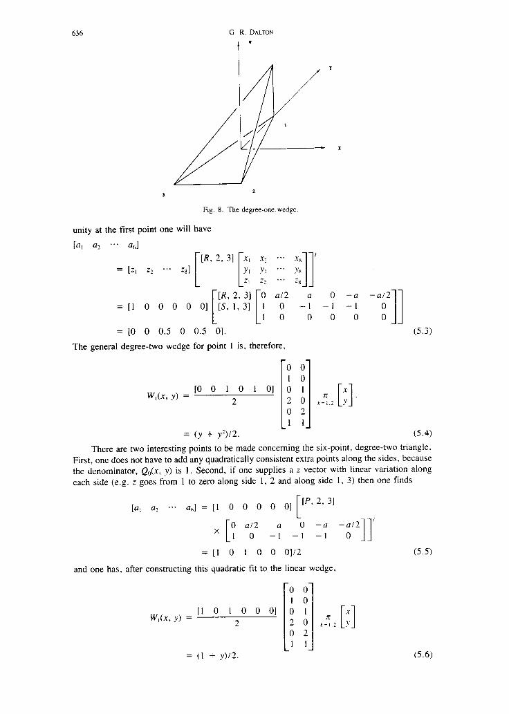
This is the expected form shown in Fig. 8. The next case is that of the degree-two wedge over a triangle. The same triangle, Fig. 7,

is used with three additional points, one at the midpoint of each side. For the wedge that is

636 G, R. DALTON

t

.

Fig. 8. The degree-one wedge.

unity at the first point one will have

[a, az *** a,]

[R, 2, 31 = [z, z2 ... zs]

x, x2 ... xg

[ 1 YI Yl ... Y8 z, z2 -.* zg

0 al2 a 0 -a -al2

=[l 0 0 0 0 O] 1 0 -1 -1 -1 0 10 000 0 11 = [O 0 0.5 0 0.5 01. (5.3)

The general degree-two wedge for point 1 is, therefore,

0 0 1 0

[O

0 1 0 1

Y) 01

0 1 x W,(& = 2 II 2 0 t=;.l [I y

0 2 1 1

= (y + y2)/2. (5.4)

There are two interesting points to be made concerning the six-point, degree-two triangle.

First, one does not have to add any quadratically consistent extra points along the sides, because the denominator, Q&X, y) is 1. Second, if one supplies a z vector with linear variation along each side (e.g. z goes from 1 to zero along side 1, 2 and along side 1, 3) then one finds

h a2 ... as] = [I 0 0 0 0 O] lP7 27 31 r I-

1

’ 0 a/2 a 0 -a -al2

x 1 0 -1 -1 -1 0 11 = [l 0 1 0 0 0]/2 (5.5)

and one has, after constructing this quadratic fit to the linear wedge,

w,(x v) = [l 0 l 0 O Ol t _ 2

= (1 + y)/2.

11 0 0 0 2 1 1 0 0 0 2 1 1 k=;.? [I x y

(5.6)

Wachspress’ rational finite element functions 637

as in Equation (5.3). One finds that the degree-one wedge is treated automatically as a subcase of the degree-two wedge in the case of a triangle and in fact for the general convex polygon.

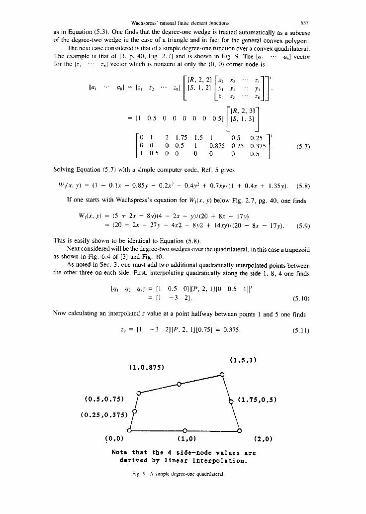
The next case considered is that of a simple degree-one function over a convex quadrilateral. The example is that of [3. p. 40, Fig. 2.71 and is shown in Fig. 9. The [a, ... ax] vector for the [z, I*. z8] vector which is nonzero at only the (0, 0) comer node is

= [I 0.5 0 0 0 0 0 0.51 [S, 1. 31

[ I

L

0 1 2 1.75 1.5 1 0.5 0.25 ’ 0 0 0 0.5 1 0.875 0.75 0.375 . 1 (5.7) 1 0.5 0 0 0 0 0 0.5

Solving Equation (5.7) with a simple computer code, Ref. 5 gives

W,(x, y) = (1 - 0.1x - 0.85~~ - 0.2~’ - 0.4~’ + 0.7@(1 + 0.4x + 1.35~). (5.8)

If one starts with Wachspress’s equation for W,(x, y) below Fig. 2.7, pg. 40, one finds

W,(x, y) = (5 + 2x - 8y)(4 - 2x - y)/(20 + 8x - 17~)

= (20 - 2x - 27y - 4x2 - 8~2 + 14xy)l(20 + 8x - 17~). (5.9)

This is easily shown to be identical to Equation (5.8). Next considered will be the degree-two wedges over the quadrilateral, in this case a trapezoid

as shown in Fig. 6.4 of [3] and Fig. 10.

As noted in Sec. 3, one must add two additional quadratically interpolated points between the other three on each side. First, interpolating quadratically along the side 1, 8, 4 one finds

14, qr 4x1 = [I 0.5 OlI]P, 2, ll]O 0.5 111’

= [l -3 21. (5.10)

Now calculating an interpolated z value at a point halfway between points 1 and 5 one finds

%I = [l -3 2][P, 2, 1][0.75] = 0.375. (5.11)

(1.5,1)

(0.5,0.75)

(0.25,0.375)

!O,O) (1,O) (2,O)

Note that the 4 side-node values are derived by linear interpolation.

Fig. 9. A simple degree-one quadrilateral.

638 G. R. DALTON

The zll and the z12 values will both be zero and zlo, halfway between points 4 and 8 will be calculated from

ZIO = [I -3 2][P, 2, 1][0.25]. (5.12)

In Fig. 10, the additional four-point locations are shown.

The wedge for degree-two approximation, that is I at point 1 and C#I at the other 7 nodes

will now be generated. The vector of fitting coefficients for this problem is

[a, a2 .** a,J = [l 0 -0.125 0 0 0 0 0 0 -0.125 0]

[R, 3, 31 -1

x [ [S,1,3] [ -1

-1 1 l-l 0 1 0 -1 0.5 1 0.5

- 1.75 11 ’

1 2 -2 0 1.5 0 -1.5 -.5 1.25 -1 1 00 0 0 0 0 0 0.375 0 0 -.I25 = [-0.375 -0.125 0 0.375 0.16667 0.16667 0.125 0 -0.16667 -0.16667 -0.3333 01.

(5.13)

Thus one has

w,(x, y) = (-0.375 - 0.125x + 0.375~’ .** -0/16667_ry?)/( I + 0.3333~). (5.14)

Examination of Eq. 6.6 of [3] yields

w,(x, y) = -3(1 - x)(x + 3 - 2y)(l + x - 2y/3)/(8(3 + x)). (5.15)

shows that Q, = - 3 * 3 * l/(8 * 3) = -0.375. Similar agreement is obtained for the other

coefficients. For z nonzero (= 1) at side-node 6 one interpolates with

192 % q31 = 10 1 Ol[[p, 29 I][0 0.5 l]]’ = [O 4 -41.

Interpolated values are calculated for the l/4 and 314 points using

i.79 znl = [O 4 -4][P, 2, 1][0.25 0.751

= [0.75 0.751.

(5.16)

(5.17)

(1,2)

(1,O)

(l,-2)

o indicate nodes with given values x indicate nodes with interpolated values

Fig. IO. A degree-two quadrilateral.

Wachspress’ rational finite element functions 639

It would seem that the stage is now set to solve for the ten coefficients that determine

P3(x, y) and the two additional coefficients in the denominator Q,(x, y) of the degree-two wedge:

W,(x, Y) = f,(x, y)lQ,(x, y) (5.18)

over the quadrilateral of Fig. 10. However, if one tries to solve Equations (3.16) one finds that the general inverse of [A] times [A] is not equal to the identity matrix [I], and one must conclude that the problem is ill conditioned. It is known from determination of the 12 coefficients for the unit comer-wedge, Eq. (5.13), that a,, = -0.3333 and ui2 = 0.

A simple resolution of this dilemma is obtained by reducing Q,(x, y) to (1 - a,,~) by the simple expedient of removing the eleventh line (1 0 1) from the power matrix and solving

for [a] less u,~. A more complete resolution is obtained by the use of the previous comer-node solution to specify all of the unknown coefficients in Q,(x, y). Thus one can rephrase the problem as

(5.19)

One then only solves for a, through ulO.

The basic flaw in the degree-one quadrilateral unit wedge for a lateral node is that nonzero information is given only along a single line in (x, y) space and this is not sufficient to determine

the denominator Q,(x, y) which is the general equation of a line in (x, y) space. Taking the approach of excluding ur2 one has

[a, a2 ... a,,] = [0.5 0.16667 -0.3333 -0.5 0 0

-0.16667 0 0.3333 0 -0.33331. (5.20)

These coefficients are in exact agreement with the terms of W&, y) of [3, p. 182, Eq. 6.61. It should be mentioned in passing that the method works equally well for the more general quadrilateral and is in no way restricted to the trapezoid.

Wachspress points out that the theoretical key to resolving this dilemma is to require that Q(x, y) pass through all of the EIP’s for which the interpolation data do not yield double values for the interpolant.

Two additional degree-one functions, over the plane pentagon and hexagon well be pre-

sented as a conclusion to the plane figures. The degree-one function for a pentagon is given

by

W(x, y) = P,(x, YYQAx, Y). (5.21)

Here the points are given on four comer plus two linearly interpolated points on each side. The four linearly related points along each side assure that the function P,(x, y)lQ,(x, y) will in fact reduce to a degree-one function along each side.

Recalling the problem encountered with the quadrilateral when z values were nonzero along one line it is not surprising to find that the pentagon, which has a degree-two denominator, QZ(x, y), cannot be determined just by nonzero z values specified along only two lines. One may impose side conditions on Q(x~ y) which yield Q(al1 EIP’s) = 0 as suggested by Wachs- press. Alternatively one may specify Z, values that are nonzero and linear on three sides around the pentagon. A toothed set of Z’S works very well (since this results in double values at the five EIP’s) to determine all of the u,‘s including the a,, to u,~ which govern the denominator,

Q:(x, y). For the general five-sided polygon one can evaluate the Q?(x, y) in this manner, and then evaluate the P3(x, y) coefficients for the particular set of five z values desired. For the

640 G. R. DALTON

equilateral pentagon it was sufficient to restrict the denominator to have only four of the five possible terms in Q2(x, y), excluding any term except the x or _v squared terms. This is because the Qz(x, y) is uniquely determined by the circle containing the exterior intersection points. Thus one will have

Qdx, y) = I - (x’ + y’)/(rq, (5.22)

where r is the radius of the circle through the external intersection points. The hexagon is treated in exactly the same fashion with no further difficulties and seems

to warrant no further comment. The degeneracy of the linear algebraic calculation of the fitting coefficients or the [a]

vector that contains the coefficients of P N+T-2(~, y) and Q,,-J-r, y) in the expression

Wik Y) = P,v+T-AX, y)lQ,v-d-x, y) (5.23)

can be better understood if one considers a specific case, such as the degree-one quadrilateral

with z values specified at the four vertices. The general equation for the z value at any point

(x, Y) is

PAX, Y) = zQ,(x, Y) (5.24)

then

a, + u2x + u3y + u4x2 + u5y2 + u6xy = z(1 - u-ix - u8y). (5.25)

If z happens to have some simple functional dependence on x and or y, then one can solve the system only for certain combinations of coefficients. For example, if z = x, then one can only find (a, + a,) and (a6 + aa). In this case there is no multiplicity so one can choose a, = a, = 0. There are only six independent coefficients.

One way out of this dilemma is to use a set of z values that are unlikely to belong to a simple function of (x, y). For example, one can use z values that are alternately + 1 and - 1 at points around the polygon. This set may then be used to determine a full set of eight values for the [a] vector. For the extremely unlikely case of this + / - 1 choice leading to a single value at an EIP, and thus to a nonunique Q(x, y) one could likely use randomly selected values between + 1 and - 1 in place of the simple + / - 1 values at the nodes.

Then one takes the two coefficients, u, and a,, which govern the denominator Qz(x, y) which is in turn governed by the N - 2 external intersection points which remain fixed and independent of z values used. After u, and a, are found using a set of + 1 or - 1 z values to calculate the [a] for a general set of z values one need only determine the six values,

[a, a2 **- q,]. This can be done using

[a, a2 ... U6] [“j *, 21 [;: ;; 1:: ::]1 =

[I - a7 - u,][P, 1, 21 [

X’ x2 ... x8 . yt YI ... Ys 1

This can be solved by post multiplying by the general inverse of

[“Y *, 2’ [;: ;; 1:: ;-]I.

(5.27)

The reconstruction of z(x, y) follows as before. The same procedure is followed for the pentagon, hexagon etc.

Wachspress’ rational finite element functions

6. EXTENSIONS OF THE WORK

641

Two classes of problems remain that want for numerical investigation. The first is the

polygon with one, or more, curved conic sides, called a polycon. Preliminary numerical in- vestigations indicate that the advantage of allowing a curved side on the element introduces (resolvable) theoretical and computational difficulties and such elements are recommended only

where a rigorous representation of a curved boundary is required. The second really challenging problem is that of the construction of a three-dimensional

element that is bounded by eight comers, roughly forming a rectangular parallelepiped, with edges that are straight lines and with faces that will be, in particular, quadric surfaces (hyper- boloids of one sheet). This “warped” parallelepiped occurs when one attempts to subdivide a three-dimensional space that has nonrectangular boundaries using points and straight lines rather

than the more cumbersome planes. The surfaces may also be further warped by the relaxation of the location of grid points as seen in [7] to give reasonably sized and shaped elements while recognizing and avoiding the difficulty of maintaining plane surfaces during relaxation. From one point of view one can project any of these warped surfaces onto any convenient plane, roughly parallel to the surface. The surface is now the simple function

c = Pz(x, y)lQ,(x, y) (6.1)

in an (x, y) coordinate system in the plane of projection. From dn alternate view point, Wachs- press suggests that these surfaces may be closely related to the Steiner surfaces discussed by McLeod[8].

Acknowledgements-Many very helpful conversations with Eugene Wachspress are gratefully acknowledged. The interest and participation of several groups of students in the course in Numerical Methods in the Dept. of Nuclear Engineering Sciences at the University of Florida is also very much appreciated.

I.

2.

3. 4.

5.

6. 7.

8.

REFERENCES

C. Lecot, Spatial Convergence Properties of Some Characteristic Methods for the SN Equations in (x. y)-Geometry. Proceedings of the ANS Topical Meeting on Advances itI Reactor Computations, Salt Lake City, Utah, March 28- 31, 1983. R. Pattemoster. A Linear Characteristic-Nodal Transport Method for the Two-Dimensional (x, y)-Geometry Mul- tigroup Discrete Ordinates Equations Over An Arbitrary Traigle Mesh. Ph.D. Dissertation, Department of Nuclear Engineering Sciences, University of Florida, Gainesville, 1983. E. Wachspress, A Rational Finite Element Basis. Academic Press, New York (1975). R. E. Cline, Elements of the Theory of the Generalized Inverses of Matrices, edc/umap, 55 Chapel St., Newton, Mass., 02160. 1979. G. R. Dalton, SUPERPOLY A Generalized Polynomial Fitting Program. Dept. of Nut. Eng. Sci., U. of Florida, Gainesville, FI., 3261 I, 1983. F. Scheid, Theo? and Problems of Numerical Ana/vsis, Shawm’s Outline Series. McGraw Hill, New York (1968). M. A. Yerry and M. S. Shephard, A Modified Quadtree Approach To Finite Element Mesh Generation, Computer Graphics. IEEE, Los Alamitos, Ca., pg. 39-46, January/February 1983. R. J. Y. McLeod, The Steiner surface revisited. Proc. R. Sot. London A369. 157-174 (1979).