Automatic Guided Vehicle Simulation in MATLAB by Using ...

17

Automatic Guided Vehicle Simulation in MATLAB by Using Genetic Algorithm

Anibal Azevedo State University of São Paulo

Brazil

1. Introduction

The prodigious advances in robotics in recent times made the use of robots more present in

modern society. One important advance that requires special attention is the development

of an unmanned aerial vehicle (UAV), which allows an aircraft to fly without having a

human crew on board, although the UAVs still need to be controlled by a pilot or a

navigator.

Today’s UAVs often combine remote control and computerized automation in a manner

that built-in control and/or guidance systems perform deeds like speed control and flight-

path stabilization. In this sense, existing UAVs are not truly autonomous, mostly because

air-vehicle autonomy field is a recently emerging field, and this could be a bottleneck for

future UAV development.

It could be said that the ultimate goal in the autonomy technology development is to replace

human pilots by altering machines decisions in order to make decisions like humans do. For

this purpose, several tools related with artificial intelligence could be employed such as

expert systems, neural networks, machine learning and natural language processing

(HAYKIN, 2009). Nowadays, the field of autonomy has mostly been following a bottom-up

approach, such as hierarchical control systems (SHIM, 2000).

One interesting methodology from the hierarchical control systems approach is the

subsumption architecture that decomposes complicated intelligent behavior into many

“simple” behavior modules, which are organized into layers. Each layer implements a

particular goal and higher layers are increasingly more abstract. The decisions are not taken

by a superior layer, but by listening to the information that are triggered by sensory inputs

(lowest layer). This methodology allows the use of reinforcement learning to acquire

behavior with the information that comes with experience.

Inspired by old behaviorist psychology, reinforcement learning (RL) concerned with how

an agent ought to take actions in an environment, so as to maximize some notion of

cumulative reward. Reinforcement learning differs from standard supervised learning in

that correct input/output pairs which are never presented (HAYKIN, 2009). Furthermore,

there is a focus on an on-line performance, which involves finding a balance between

exploration (of uncharted territory) and exploitation (of current knowledge). The

reinforcement learning has been applied successfully to various problems, including robot

control, elevator scheduling, telecommunications, backgammon and chess (SHIM, 2000).

www.intechopen.com

MATLAB for Engineers – Applications in Control, Electrical Engineering, IT and Robotics 410

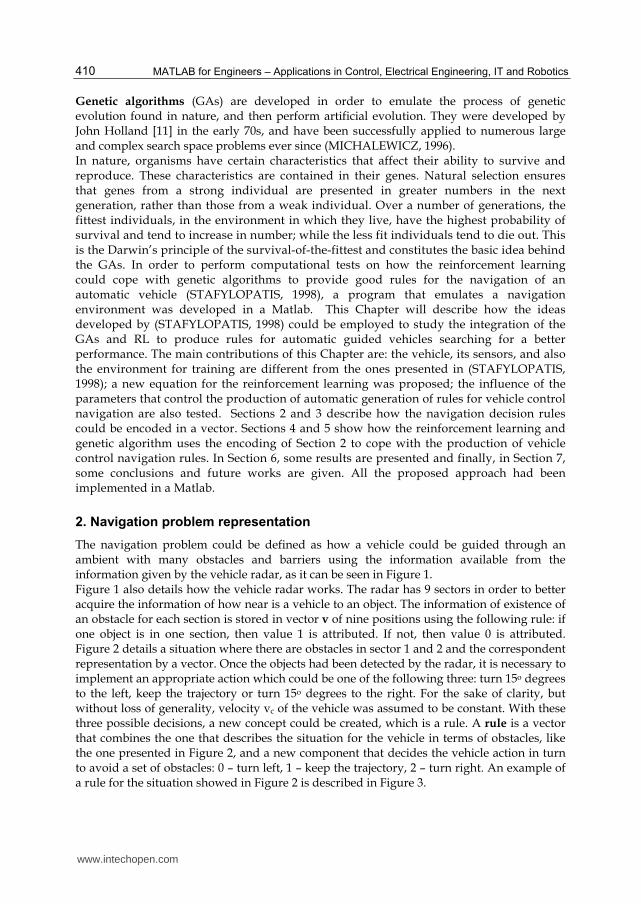
Genetic algorithms (GAs) are developed in order to emulate the process of genetic evolution found in nature, and then perform artificial evolution. They were developed by John Holland [11] in the early 70s, and have been successfully applied to numerous large and complex search space problems ever since (MICHALEWICZ, 1996). In nature, organisms have certain characteristics that affect their ability to survive and reproduce. These characteristics are contained in their genes. Natural selection ensures that genes from a strong individual are presented in greater numbers in the next generation, rather than those from a weak individual. Over a number of generations, the fittest individuals, in the environment in which they live, have the highest probability of survival and tend to increase in number; while the less fit individuals tend to die out. This is the Darwin’s principle of the survival-of-the-fittest and constitutes the basic idea behind the GAs. In order to perform computational tests on how the reinforcement learning could cope with genetic algorithms to provide good rules for the navigation of an automatic vehicle (STAFYLOPATIS, 1998), a program that emulates a navigation environment was developed in a Matlab. This Chapter will describe how the ideas developed by (STAFYLOPATIS, 1998) could be employed to study the integration of the GAs and RL to produce rules for automatic guided vehicles searching for a better performance. The main contributions of this Chapter are: the vehicle, its sensors, and also the environment for training are different from the ones presented in (STAFYLOPATIS, 1998); a new equation for the reinforcement learning was proposed; the influence of the parameters that control the production of automatic generation of rules for vehicle control navigation are also tested. Sections 2 and 3 describe how the navigation decision rules could be encoded in a vector. Sections 4 and 5 show how the reinforcement learning and genetic algorithm uses the encoding of Section 2 to cope with the production of vehicle control navigation rules. In Section 6, some results are presented and finally, in Section 7, some conclusions and future works are given. All the proposed approach had been implemented in a Matlab.

2. Navigation problem representation

The navigation problem could be defined as how a vehicle could be guided through an ambient with many obstacles and barriers using the information available from the information given by the vehicle radar, as it can be seen in Figure 1. Figure 1 also details how the vehicle radar works. The radar has 9 sectors in order to better acquire the information of how near is a vehicle to an object. The information of existence of an obstacle for each section is stored in vector v of nine positions using the following rule: if one object is in one section, then value 1 is attributed. If not, then value 0 is attributed. Figure 2 details a situation where there are obstacles in sector 1 and 2 and the correspondent representation by a vector. Once the objects had been detected by the radar, it is necessary to implement an appropriate action which could be one of the following three: turn 15o degrees to the left, keep the trajectory or turn 15o degrees to the right. For the sake of clarity, but without loss of generality, velocity vc of the vehicle was assumed to be constant. With these three possible decisions, a new concept could be created, which is a rule. A rule is a vector that combines the one that describes the situation for the vehicle in terms of obstacles, like the one presented in Figure 2, and a new component that decides the vehicle action in turn to avoid a set of obstacles: 0 – turn left, 1 – keep the trajectory, 2 – turn right. An example of a rule for the situation showed in Figure 2 is described in Figure 3.

www.intechopen.com

Automatic Guided Vehicle Simulation in MATLAB by Using Genetic Algorithm 411

Fig. 1. Description of the elements of the developed environment in Matlab.

Situation

1

1

0

0

0

0

0

0

0

Vector Index

0

1

2

3

4

5

6

7

8

Sector 1 2 3 4 5 6 7 8 9

Fig. 2. The correspondence between the obstacles detected by a radar vehicle and a vector with binary information.

Fig. 3. The correspondence between a rule and decision taken by the vehicle.

www.intechopen.com


3. Navigation control

The previous binary representation scheme has a main drawback since before every vehicle

movement decision demanded to store 3×29 = 1536 vectors (rules) to precisely describe which action should be performed for each scenario detected by the radar information. This implies that before every step performed by the vehicle, a control action should compare, in the worst case, 1536 vectors in order to find the proper decision to be taken. This scheme is illustrated in Fig. 4.

Fig. 4. Decision scheme followed by the automatic guided vehicle.

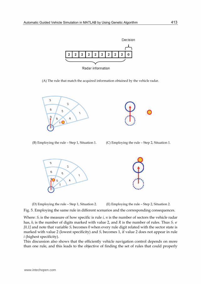
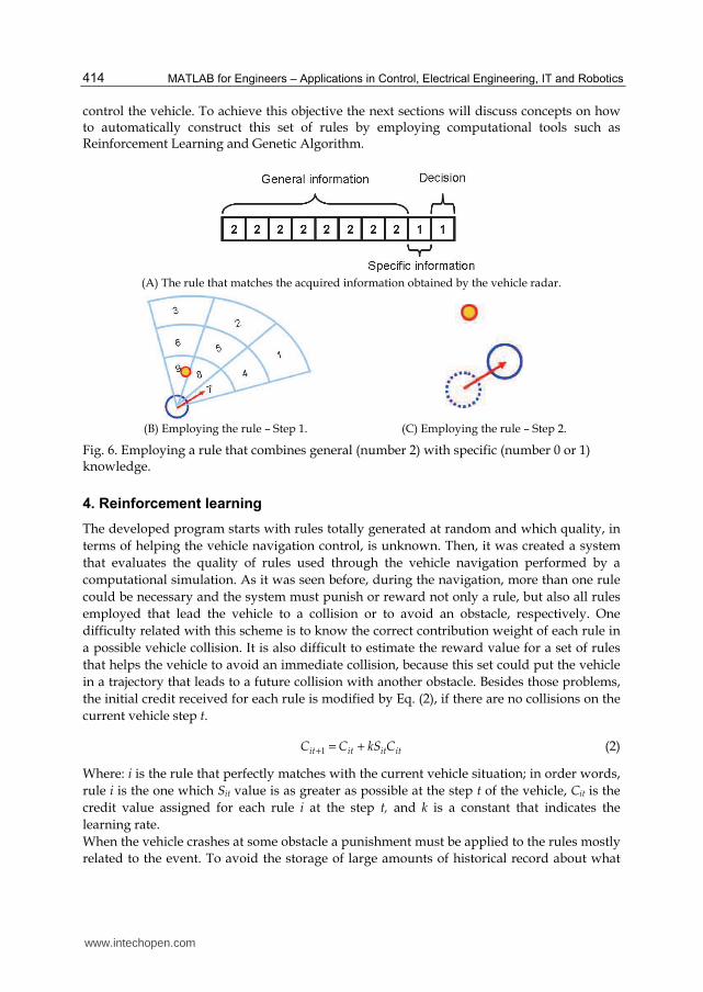
This computational work could be avoided by introducing a new symbol 2, for the radar information section, which means that “it could have or not an obstacle at this sector”. The advantage of the definition of this new symbol is that it will help to reduce the number of necessary information to be kept by the vehicle control. The disadvantage of using this new symbol is that it could group different situations where the decisions should not be the same. Fig. 5 gives an example of this situation. The example showed in Fig. 5 emphasizes the importance to construct the rules in a manner that the parts of the rule which do not affect the decision should be numbered as 2, and the other parts that have a great influence in the final behavior of the vehicle should be numbered as most specific as possible or, in other words, with the numbers 0 or 1. Fig. 6 illustrates the application of this concept. Fig. 6 also gives a guideline procedure for another problem that could emerge, which is the appearance of more than one rule that matches the current radar information when symbol 2 is used. One criteria that will be adopted is to select the rules which match the environment situation, but with as much specific information as possible. For this purpose Eq. (1) will be adopted.

( )ii

n kS

n

−= 1, ,i R= (1)

www.intechopen.com


(A) The rule that match the acquired information obtained by the vehicle radar.

(B) Employing the rule – Step 1, Situation 1. (C) Employing the rule – Step 2, Situation 1.

(D) Employing the rule – Step 1, Situation 2. (E) Employing the rule – Step 2, Situation 2.

Fig. 5. Employing the same rule in different scenarios and the corresponding consequences.

Where: Si is the measure of how specific is rule i, n is the number of sectors the vehicle radar

has, ki is the number of digits marked with value 2, and R is the number of rules. Thus Si ∈

[0,1] and note that variable Si becomes 0 when every rule digit related with the sector state is

marked with value 2 (lowest specificity) and Si becomes 1, if value 2 does not appear in rule

i (highest specificity).

This discussion also shows that the efficiently vehicle navigation control depends on more than one rule, and this leads to the objective of finding the set of rules that could properly

www.intechopen.com


control the vehicle. To achieve this objective the next sections will discuss concepts on how to automatically construct this set of rules by employing computational tools such as Reinforcement Learning and Genetic Algorithm.

(A) The rule that matches the acquired information obtained by the vehicle radar.

(B) Employing the rule – Step 1. (C) Employing the rule – Step 2.

Fig. 6. Employing a rule that combines general (number 2) with specific (number 0 or 1) knowledge.

4. Reinforcement learning

The developed program starts with rules totally generated at random and which quality, in

terms of helping the vehicle navigation control, is unknown. Then, it was created a system

that evaluates the quality of rules used through the vehicle navigation performed by a

computational simulation. As it was seen before, during the navigation, more than one rule

could be necessary and the system must punish or reward not only a rule, but also all rules

employed that lead the vehicle to a collision or to avoid an obstacle, respectively. One

difficulty related with this scheme is to know the correct contribution weight of each rule in

a possible vehicle collision. It is also difficult to estimate the reward value for a set of rules

that helps the vehicle to avoid an immediate collision, because this set could put the vehicle

in a trajectory that leads to a future collision with another obstacle. Besides those problems,

the initial credit received for each rule is modified by Eq. (2), if there are no collisions on the

current vehicle step t.

1it it it itC C kS C+ = + (2)

Where: i is the rule that perfectly matches with the current vehicle situation; in order words,

rule i is the one which Sit value is as greater as possible at the step t of the vehicle, Cit is the

credit value assigned for each rule i at the step t, and k is a constant that indicates the

learning rate.

When the vehicle crashes at some obstacle a punishment must be applied to the rules mostly

related to the event. To avoid the storage of large amounts of historical record about what

www.intechopen.com


rules where used, and to punish just the rules mostly related to the collision, only the last

three employed rules will have their credit updated by Eq. (3).

1

2/it itC C+ = (3)

Eq. (3) was considered by (STAFYLOPATIS, 1998), but it represents that the rules that lead the vehicle to perform more than 200 steps without a collision will suffer the same punishment as

the rules that conduct the vehicle to perform only 20 steps without a collision, for example. To avoid this problem, this book Chapter proposes, for the first time, a punishment formula

which is a function on the number of steps as showed in Eq. (4) and (5).

1it p itC k C+ =

(4)

1

1

1( )/exp

p ns npk

− +=

+ (5)

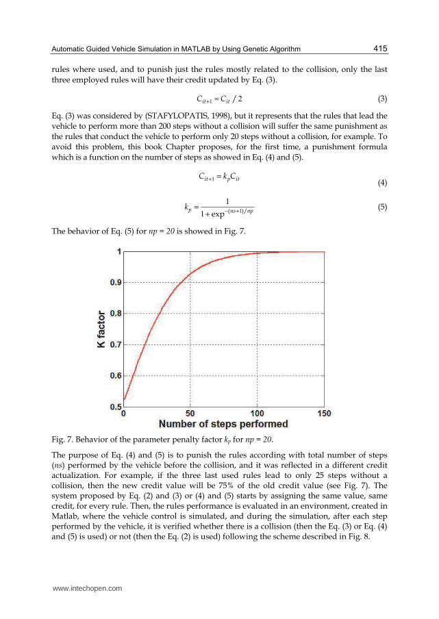
The behavior of Eq. (5) for np = 20 is showed in Fig. 7.

Fig. 7. Behavior of the parameter penalty factor kp for np = 20.

The purpose of Eq. (4) and (5) is to punish the rules according with total number of steps (ns) performed by the vehicle before the collision, and it was reflected in a different credit actualization. For example, if the three last used rules lead to only 25 steps without a collision, then the new credit value will be 75% of the old credit value (see Fig. 7). The system proposed by Eq. (2) and (3) or (4) and (5) starts by assigning the same value, same credit, for every rule. Then, the rules performance is evaluated in an environment, created in Matlab, where the vehicle control is simulated, and during the simulation, after each step performed by the vehicle, it is verified whether there is a collision (then the Eq. (3) or Eq. (4) and (5) is used) or not (then the Eq. (2) is used) following the scheme described in Fig. 8.

www.intechopen.com


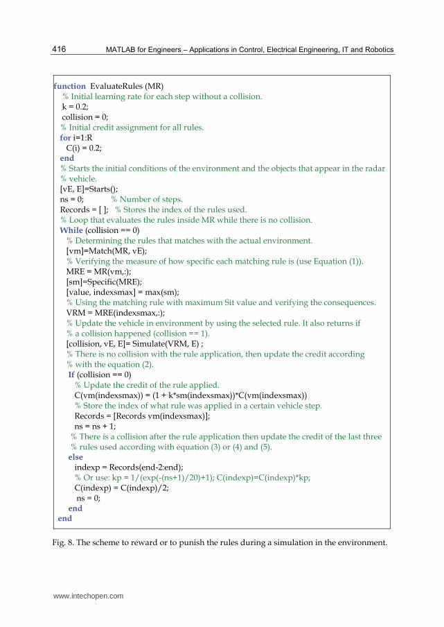
function EvaluateRules (MR) % Initial learning rate for each step without a collision. k = 0.2; collision = 0; % Initial credit assignment for all rules. for i=1:R C(i) = 0.2; end % Starts the initial conditions of the environment and the objects that appear in the radar % vehicle. [vE, E]=Starts(); ns = 0; % Number of steps. Records = [ ]; % Stores the index of the rules used. % Loop that evaluates the rules inside MR while there is no collision. While (collision == 0) % Determining the rules that matches with the actual environment. [vm]=Match(MR, vE); % Verifying the measure of how specific each matching rule is (use Equation (1)). MRE = MR(vm,:); [sm]=Specific(MRE); [value, indexsmax] = max(sm); % Using the matching rule with maximum Sit value and verifying the consequences. VRM = MRE(indexsmax,:); % Update the vehicle in environment by using the selected rule. It also returns if % a collision happened (collision == 1). [collision, vE, E]= Simulate(VRM, E) ; % There is no collision with the rule application, then update the credit according % with the equation (2). If (collision == 0) % Update the credit of the rule applied. C(vm(indexsmax)) = (1 + k*sm(indexsmax))*C(vm(indexsmax)) % Store the index of what rule was applied in a certain vehicle step. Records = [Records vm(indexsmax)]; ns = ns + 1; % There is a collision after the rule application then update the credit of the last three % rules used according with equation (3) or (4) and (5). else indexp = Records(end-2:end); % Or use: kp = 1/(exp(-(ns+1)/20)+1); C(indexp)=C(indexp)*kp; C(indexp) = C(indexp)/2; ns = 0; end end

Fig. 8. The scheme to reward or to punish the rules during a simulation in the environment.

www.intechopen.com


The functions and symbols used in Fig. 8 are defined as follows: C - Vector containing the credit associated to a set of rules. E - Matrix with all data about the current simulation environment state. vE - Vector with information extracted from the radar, as show in Figure 2. MR - Matrix with a set of rules. Each matrix line represents one rule. Vm - The vector with the index of the rules that matches the information extracted

from vehicle radar (contained in vE). MRE - Matrix with only the rules that match the information extracted from vehicle

radar. Specific - This function evaluates all the rules contained in matrix MRE according with

the equation Eq. (1) in order to measure how specific is each rule. sm - Vector with all rules specific measure. max - This function determines which specific measure is the biggest (value) and

the corresponding line of MRE (indexsmax). VRM - Vector with the rule selection to be used in current environment state. Simulate - This function simulates the vehicle through environment using VRM rules. collision - Variable that indicates whether a vehicle collides (equals to 1) or not (equals

to 0). indexsmax - Index of the rule with maximum matching value. Records - Vector that stores the index of the rules used in a certain vehicle step through

the environment. indexp - Vector with the index of the last three rules applied before the vehicle

collision and which will be punished by a credit decreasing. ns - Number of steps without a collision. kp - Penalization factor applied in the credit of the last three rules when a collision

occurs. The system showed in Fig. 8 tries to establish a reward and a punishment scheme among the rules and their impact in the vehicle navigation through equations that monitor the performance, although the random generation of rules can also produce sets of rules which lead to a bad control navigation performance. After a pre-specified number of collisions, the set of rules could be changed by a new randomly generated set of rules formed with the insertion of new rules, the exclusion of rules with a bad performance (low credit value), and the maintenance of rules that help to avoid the obstacles (high credit value). To perform the formation of this new set of rules, a genetic algorithm was coupled to the credit evaluation scheme described in Fig. 8, as could be seen in Fig.9. The complete description of the Genetic Algorithm developed is described in Section 5.

5. Genetic algorithm

The genetic algorithm keeps a population of individuals, represented by: A(t) = {A1t, ..., Ant} for each generation (iteration) t, and each individual represents a rule to guide the vehicle through the environment and to avoid the obstacles. In the computational implementation adopted here, the population is stored in a matrix A(t) and each column Ait represents a rule. Each rule Ait is evaluated according to the number of vehicle movements without a collision, and then, the fitness, a measure of how this individual is sucessful for the problem, is calculated. The fitness is calculated for the entire population and is based on this new population that combines the most capable individuals that will form generation t+1.

www.intechopen.com


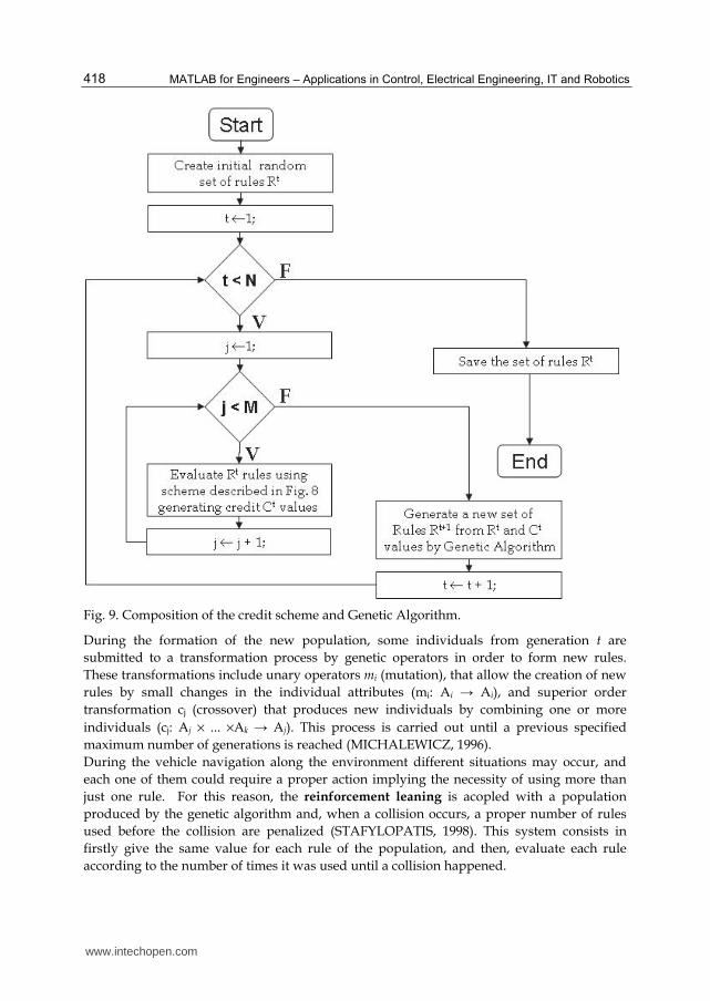
Fig. 9. Composition of the credit scheme and Genetic Algorithm.

During the formation of the new population, some individuals from generation t are

submitted to a transformation process by genetic operators in order to form new rules.

These transformations include unary operators mi (mutation), that allow the creation of new

rules by small changes in the individual attributes (mi: Ai → Ai), and superior order

transformation cj (crossover) that produces new individuals by combining one or more

individuals (cj: Aj × ... ×Ak → Aj). This process is carried out until a previous specified

maximum number of generations is reached (MICHALEWICZ, 1996).

During the vehicle navigation along the environment different situations may occur, and

each one of them could require a proper action implying the necessity of using more than

just one rule. For this reason, the reinforcement leaning is acopled with a population

produced by the genetic algorithm and, when a collision occurs, a proper number of rules

used before the collision are penalized (STAFYLOPATIS, 1998). This system consists in

firstly give the same value for each rule of the population, and then, evaluate each rule

according to the number of times it was used until a collision happened.

www.intechopen.com


The implementation details adopted for the Genetic Algorithm are as follows:

(A) Data structure codification for each individual:

Each genetic algorithm individual is associated to a rule by using a vector v with 10

elements and values inside the elements 1 to 9, corresponding to the presence (value 1) or

not (value 0) or whatever (value 2) in the corresponding vehicle radar section, respectively

(see Fig. 3). The value inside the position 10 indicates the decision that has to be made: 0 -

turn 15o degrees to the left, 1 – keep the trajectory and 2 - turn 15o degrees to the right. The

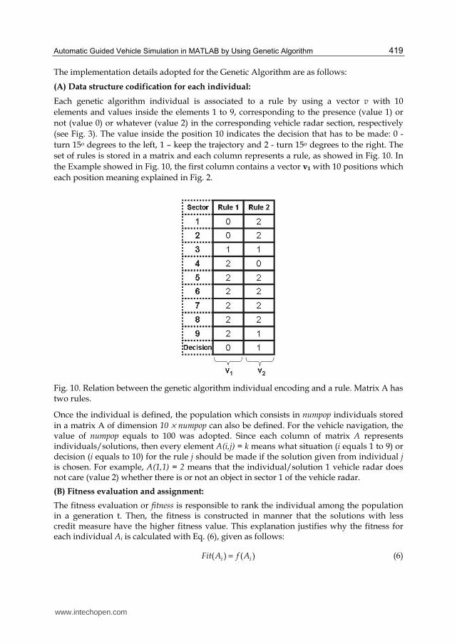
set of rules is stored in a matrix and each column represents a rule, as showed in Fig. 10. In

the Example showed in Fig. 10, the first column contains a vector v1 with 10 positions which

each position meaning explained in Fig. 2.

Fig. 10. Relation between the genetic algorithm individual encoding and a rule. Matrix A has two rules.

Once the individual is defined, the population which consists in numpop individuals stored in a matrix A of dimension 10 × numpop

can also be defined. For the vehicle navigation, the

value of numpop equals to 100 was adopted. Since each column of matrix A represents individuals/solutions, then every element A(i,j) = k means what situation (i equals 1 to 9) or decision (i equals to 10) for the rule j should be made if the solution given from individual j is chosen. For example, A(1,1) = 2 means that the individual/solution 1 vehicle radar does not care (value 2) whether there is or not an object in sector 1 of the vehicle radar.

(B) Fitness evaluation and assignment:

The fitness evaluation or fitness is responsible to rank the individual among the population in a generation t. Then, the fitness is constructed in manner that the solutions with less credit measure have the higher fitness value. This explanation justifies why the fitness for each individual Ai is calculated with Eq. (6), given as follows:

( ) ( )i iFit A f A= (6)

www.intechopen.com


Where: ( )if A is the fitness evaluation as defined by the credit value Cit, and it corresponds

to the number of steps performed with rule i without a collision, according to the rule stored in vector Ai, through the environment.

(C) Individual Selection for the next generation:

The population formation process employed is the “Roulette Wheel”, in order words, a random raffle where the probability Q(Ai) to choose the individual Ai for the next generation, in a population with b individuals, is used. The value Q(Ai) can be obtained by using Eq. (7).

1

( ) ( ) / ( ( ))numpop

i i ii

Q A Fit A Fit A=

= (7)

The better individual of the actual generation is always kept to be on the next generation.

(D) Crossover OX:

The Crossover operators try to generate new individuals to form the next population by combining information from past generations that is present in the individuals. This work used two crossover operators which is described as follows. Two individuals, A1 and A2 , with N elements are randomly chosen from a population in generation t. Then, an integer number δ in the interval [1, N-1] is drawn and elements of A1 that are in positions δ until N are exchanged with the elements of A2 that are in positions δ until N. This exchange will produce two new individuals, nA1 and nA2, that can appear in the next generation.

(E) Mutation operator:

The mutation operator modifies 10*numpop*pm elements of matrix A, where pm is the percentage of total bits to be muted (mutated). The selection of which element Aij to be mutated consist in randomly select the line index and the column index, and then change it. Fig. 11 shows how the genetic algorithm components described before are combined. One important observation is that the best individual of generation At is always kept for the next generation At+1. Furthermore, the size of subpopulations As1t and As2t are the same and is equal to 5% of the total population (numpop).

Fig. 11. How the genetic algorithm elements are combined into a unique algorithm.

www.intechopen.com


6. Tests and results

Table 1 sumarizes the description of the parameters necessary to perform tests with the developed approach described in sections 4 and 5.

Parameter DescriptionCi0 Initial credit assigment for a set of rules.k reinformecent learning rate parameter.pb0 percentance of digits equals to 0 for the initial population. pb1 percentance of digits equals to 1 for the initial population. pb2 percentance of digits equals to 2 for the initial population. numpop number of individuals in the genetic algorithm population. pc Crossover rate.pm Mutation rate.pg size of the subpopulation in terms of the A matrix (5%).M number of collisions before applying the genetic algorithm (10). N number of genetic algorithm aplication(14).

Table 1. Parameters used for the developed approach and their meanings.

It was also tested two environments whose obstacles initial position are shown in Fig. 12. As shown in Fig. 12, the obstacles could be clustered in two groups: the obstacles that delimits the environment bounds have their position fixed and the obstacles that are in the interior of the environment, whose positions are actualized in a different manner for each environment: • Environment 1: The moving obstacles actualize their x-positions according to Eq. (8).

t ti ix x ε= + (8)

Where: xit is the x-position for obstacle i in step t of the vehicle, ε is a random uniform variable in the interval [0, 1].

Fig. 12. Detailed description of the obstacles initial position in the environment.

www.intechopen.com


• Environment 2: The user could also specify a positive value to a radius parameter and the moving obstacles actualize their x and y-positions according to Eq. (9).

* cos( )

* sin( )

t t ti i i

t t ti i i

x x radius x

y y radius y

= +

= + (9)

For all tests performed in environment 2, the radius value was fixed in 5. Five runs with the values listed in Table 2 had been performed in order to carry the best set of values for all the parametes listed in Table 1. Each row in Table 2 corresponds to a new configuration.

Set Ci0 k Pb0 Pb1 Pb2 numpop pc pm pg M N Environment

1 20 2 2.5% 2.5% 95% 100 30 1 5 10 14 1

2 20 2 2.5% 2.5% 95% 100 1 30 5 10 14 1

3 20 2 2.5% 2.5% 95% 100 30 1 5 20 5 1

4 20 2 2.5% 2.5% 95% 100 1 30 5 20 5 1

5 20 2 10% 10% 80% 100 30 1 5 20 5 1

6 20 2 10% 10% 80% 100 1 30 5 20 5 1

7 20 2 2.5% 2.5% 95% 100 1 30 5 20 5 2

8 20 2 10% 10% 80% 100 30 1 5 20 5 2

Table 2. List of values assigned for each parameter.

Each row of Table 3 corresponds to the number of the steps that could be taken with the final set of rules obtained after the application of the scheme described in Fig. 9 using the parameters described in Table 2 and the reinforcement learning that follows Eq. (3).

Set Test 1 Test 2 Test 3 Test 4 Test 5Best

Number

1 16 7 7 7 7 16

2 7 110 7 7 80 110

3 28 57 78 16 7 78

4 177 32 48 21 18 177

5 151 18 15 32 116 151

6 34 32 19 32 106 106

7 32 163 20 106 84 163

8 38 15 31 108 31 108

Table 3. The number of maximum steps without a collision performed by the best set of

rules produced by each set of parameters (described in Table 2) and Eq. (3).

In Table 3, the first column indicates the set of parameters and the corresponding obtained set of rules which lead to the number of maximum steps without a collision described in the second column until the sixth column. The results for the set of parameters 1 to 6 show that for environment 1 the best choices of parameters are sets 4 and 5. Those two sets were also tested in environment 2 in order to verify set parameters robustness in order to produce adequate rules for different environments. Configuration 7 had the best performance and three tests were sucessfull in producing rules which could make the vehicle able to take more than 80 steps without a collision.

www.intechopen.com


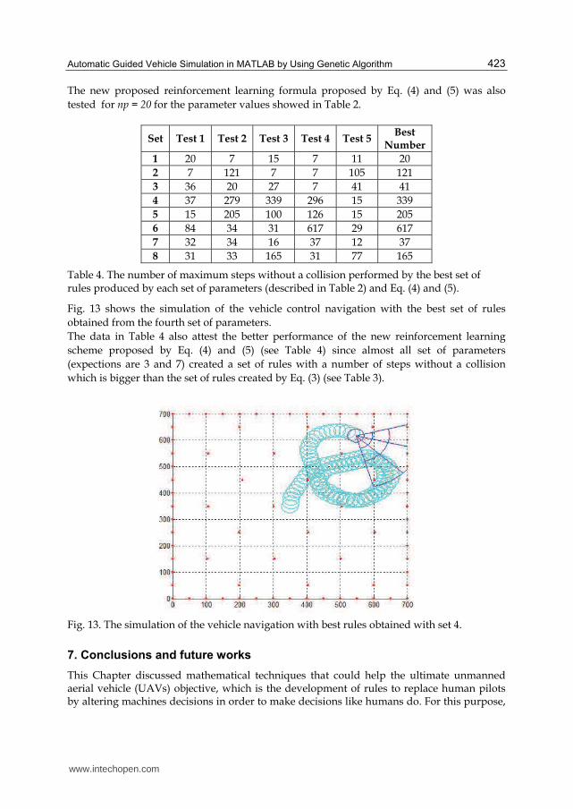
The new proposed reinforcement learning formula proposed by Eq. (4) and (5) was also

tested for np = 20 for the parameter values showed in Table 2.

Set Test 1 Test 2 Test 3 Test 4 Test 5Best

Number

1 20 7 15 7 11 20

2 7 121 7 7 105 121

3 36 20 27 7 41 41

4 37 279 339 296 15 339

5 15 205 100 126 15 205

6 84 34 31 617 29 617

7 32 34 16 37 12 37

8 31 33 165 31 77 165

Table 4. The number of maximum steps without a collision performed by the best set of rules produced by each set of parameters (described in Table 2) and Eq. (4) and (5).

Fig. 13 shows the simulation of the vehicle control navigation with the best set of rules

obtained from the fourth set of parameters.

The data in Table 4 also attest the better performance of the new reinforcement learning

scheme proposed by Eq. (4) and (5) (see Table 4) since almost all set of parameters

(expections are 3 and 7) created a set of rules with a number of steps without a collision

which is bigger than the set of rules created by Eq. (3) (see Table 3).

Fig. 13. The simulation of the vehicle navigation with best rules obtained with set 4.

7. Conclusions and future works

This Chapter discussed mathematical techniques that could help the ultimate unmanned aerial vehicle (UAVs) objective, which is the development of rules to replace human pilots by altering machines decisions in order to make decisions like humans do. For this purpose,

www.intechopen.com


several tools related with artificial intelligence could be employed such as expert systems, neural networks, machine learning and natural language processing (HAYKIN, 2009). Two methodologies, reinforcement learning and genetic algorithms, are described and combined. The methodologies had been implemented in a Matlab and were successfully applied in order to create rules that keep the vehicle away from the obstacles from random initial rules. This Chapter also described how the ideas developed by (STAFYLOPATIS, 1998) could be modified, particularly the setting of parameters and a new reinforcement learning methodology, to provide a better integration of the Genetic Algorithms (GAs) and Reinforcement Learning (RL) which produce rules for automatic guided vehicles with a better performance. The main contributions of this Chapter were: the vehicle, its sensors, and also the environment for training which are different from the ones presented in (STAFYLOPATIS, 1998); a new equation for the reinforcement learning was proposed; the influence of the parameters that control the production of automatic generation of rules for vehicle control navigation are also tested. The results presented attested the better performance of the new reinforcement learning scheme proposed, implemented in Matlab. For future works, it could be applied a genetic algorithm for finding the better configuration of the parameters for the combined scheme of reinforcement learning and the genetic algorithm used to find the rules. For future works more tests could be performed by using other equations for the reinforcement learning process and also other methods like Beam Search (SABUNCUOGLU and BAVIZ, 1999; DELLA CROCE and T’KINDT, 2002) could replace the Genetic Algorithm. A more detailed and complex decisions could also be incorporated such as the possibility of increasing or reducing the velocity of the vehicle.

8. References

Della Croce, F.; T’Kind, V., A Recovering Beam Search Algorithm for the One-Machine Dynamic Total Completation Time Scheduling Problem, Journal of the Operational Research Society, vol. 54, p. 1275-1280, 2002.

Haykin, , S. Neural Networks and Learning Machines, 3rd edition, Prentice Hall, 2009. Sutton, R.S., Barto, A.G., Reinforcement Learning: An Introduction, MIT Press, 1998. Stafylopatis, A., Blekas, K., Autonomous vehicle navigation using evolutionary

reinforcement learning, European Journal of Operational Research, Vol. 108(2), p. 306-318, 1998.

Shim, D. H, Kim, H. J., Sastry, S., Hierarchical Control System Synthesis for Rotorcraft-based Unmanned Aerial Vehicles, AIAA Guidance, Navigation, and Control Conference and Exhibit, v. 1, p. 1-9, 2000.

Holland, J. H., Adaptation in natural and artificial systems. The University of Michigan Press, 1975.

Michalewicz, Z. Genetic Algorithms + Data Structures = Evolution Programs, 3rd edition, Springer-Verlag, 1996.

Sabuncuoglu, I., Baviz, M., Job Shop Scheduling with Beam Search, European Journal of Operational Research, vol. 118, pp. 390-412.

www.intechopen.com

MATLAB for Engineers - Applications in Control, ElectricalEngineering, IT and RoboticsEdited by Dr. Karel Perutka

ISBN 978-953-307-914-1Hard cover, 512 pagesPublisher InTechPublished online 13, October, 2011Published in print edition October, 2011

InTech EuropeUniversity Campus STeP Ri Slavka Krautzeka 83/A 51000 Rijeka, Croatia Phone: +385 (51) 770 447 Fax: +385 (51) 686 166www.intechopen.com

InTech ChinaUnit 405, Office Block, Hotel Equatorial Shanghai No.65, Yan An Road (West), Shanghai, 200040, China

Phone: +86-21-62489820 Fax: +86-21-62489821

The book presents several approaches in the key areas of practice for which the MATLAB software packagewas used. Topics covered include applications for: -Motors -Power systems -Robots -Vehicles The rapiddevelopment of technology impacts all areas. Authors of the book chapters, who are experts in their field,present interesting solutions of their work. The book will familiarize the readers with the solutions and enablethe readers to enlarge them by their own research. It will be of great interest to control and electrical engineersand students in the fields of research the book covers.

How to referenceIn order to correctly reference this scholarly work, feel free to copy and paste the following:

Anibal Azevedo (2011). Automatic Guided Vehicle Simulation in MATLAB by Using Genetic Algorithm, MATLABfor Engineers - Applications in Control, Electrical Engineering, IT and Robotics, Dr. Karel Perutka (Ed.), ISBN:978-953-307-914-1, InTech, Available from: http://www.intechopen.com/books/matlab-for-engineers-applications-in-control-electrical-engineering-it-and-robotics/automatic-guided-vehicle-simulation-in-matlab-by-using-genetic-algorithm

© 2011 The Author(s). Licensee IntechOpen. This is an open access articledistributed under the terms of the Creative Commons Attribution 3.0License, which permits unrestricted use, distribution, and reproduction inany medium, provided the original work is properly cited.

http://creativecommons.org/licenses/by/3.0

Automatic Guided Vehicle Simulation in MATLAB by Using ...

Documents

Transcript of Automatic Guided Vehicle Simulation in MATLAB by Using ...