Automatic Grid Generation - · PDF fileAutomatic Grid Generation William D. Henshaw...

Acta Numerica (1996), pp. 1–??

Automatic Grid Generation

William D. Henshaw

Scientific Computing Group

Computing, Information and Communications Division

Los Alamos National Laboratory

Los Alamos, NM, 87545

Current methods for the automatic generation of grids are reviewed. Theapproaches to grid generation that are discussed include cartesian, multi-block-structured, overlapping and unstructured. Emphasis is placed on thosemethods that can create high-quality grids appropriate for the solution ofequations with a hyperbolic nature such as those that arise in fluid dynamics.Numerous figures illustrate the different grid generation techniques.

CONTENTS

1 Introduction 12 Basic Steps in Grid Generation 73 Cartesian Grid Generation 84 Multi-Block-Structured Grid Generation 105 Overlapping Grid Generation 156 Unstructured Grid Generation 157 Conclusions 23References 25

1. Introduction

The intent of this paper is to give a brief review of current methods forthe automatic generation of grids for the solution of problems from compu-tational fluid dynamics (CFD), computational electromagnetics and otherfields where the solutions are hyperbolic in nature. These applications re-quire the generation of high quality grids with a large number of grid points.It is often the case that the geometry may change with time or it may benecessary to adaptively refine the mesh. It is thus essential that the gridgeneration algorithms be fast since the grid may have to be regenerated atevery step of a time dependent simulation. Various popular methods forstructured and unstructured grid generation will be described. Figures will

2 William D. Henshaw

illustrate the current state of the technology. Grid generation capabilitieshave improved greatly in recent years. However, it is perhaps not an exag-geration to say that the construction of a grid is currently the most difficultand time consuming aspect in determining an accurate solution to a problemon a complicated domain. Indeed, starting from scratch with some descrip-tion of the geometry the time to generate a grid is measured in weeks ratherthan hours.

Fig. 1. Early grids represented geometry using a cartesian (cut-out) grid.

cut-out grids) whereby the region was covered by a single rectangulargrid and the portions of the grid lying outside the region were cut-out leav-ing some irregularly spaced cells. This approach was replaced by boundaryconforming grids whereby a logically rectangular grid was mapped onto theregion, with boundaries corresponding to a coordinate line. Grids that con-formed to boundaries improved solution accuracy and made it easier toapply boundary conditions. As computers became faster and more compli-cated problems were attempted it became apparent that this single-blockapproach was not flexible enough to handle complicated geometries. Thisled to the introduction of the multi-block approach where the domain waspartitioned into blocks and within each block a logically rectangular gridwas constructed. In time, however, it became apparent that this approachwas still not flexible enough (and difficult to automate) for the increasinglycomplex geometries being considered and some other approach was needed.One way to add additional flexibility, while still retaining the logically rect-

Automatic Grid Generation 3

Fig. 2. A multi-block structured grid divides the region into logically rectangularblocks.

angular structure was the use of overlapping grids in which the componentgrids are allowed to overlap. There has also been renewed interestin the cartesian grid approach, using adaptive mesh refinement to improveboundary resolution. Recently the main interest and focus of research hasbeen in unstructured meshes, which allow complete freedom in grid pointplacement, although at the expense of speed and memory usage. With littledoubt, unstructured meshes offer the best hope for a completely automaticmesh generation program. Completely unstructured grids are not withouttheir difficulties for CFD and perhaps a hybrid method, combining the un-structured approach with locally structured grids (to resolve boundary layersfor example) will turn out to be most the effective.

The purpose of grid generation is to create a discrete representation fora domain. This entails distributing points throughout the domain. Thereare two main classes of grids, structured and unstructured. In a structuredgrid the points covering the domain result from the transformation of alogically rectangular square (or cube in three dimensions∗). The grid pointscan be stored as an array x(i1, i2) and the neighbours of a given grid pointare simply found as the neighbours in index space, x(i1 ± 1, i2 ± 1). Inan unstructured grid, on the other hand, the points are connected to one

∗ Throughout this paper, the terminology will be for two-dimensional grids, (quadrilat-erals, triangles) but the remarks will usually apply equally well to three-dimensionalgrids (hexahedra, tetrahedra)


Fig. 3. An overlapping grid consists of logically rectangular blocks that overlap,some blocks have cut-out regions.

another in a general manner, the connectivity information must be explicitlysaved. The grid points might be saved as a list xi, and there would be otherlists giving information about neighbours. Of course, the partition of gridstypes into structured and unstructured is not entirely appropriate since somegrids consist of a set of structured grids and other hybrid grids have bothunstructured and structured parts.

Grids are used to solve equations, typically partial differential equations(PDEs) and integral equations. The computer programs that solve theseequations, which are here-in referred so as solvers, typically discretize a con-tinuous equation with finite-difference, finite-element, finite-volume, spectral-element or boundary-integral methods. At the grid generation level, it isusually not important which particular solver will use the grid, rather thestyle of the grid is most relevant. That is, it is important whether the gridis structured or unstructured, whether the grid elements are triangles orquadrilaterals, or whether the grid is multi-block-structured or overlapping.The unstructured triangular grid can be used either with a finite-elementsolver or a finite-volume solver, just as a multi-block-structured grid canbe used by a finite-difference solver or by finite-element solver for quadri-


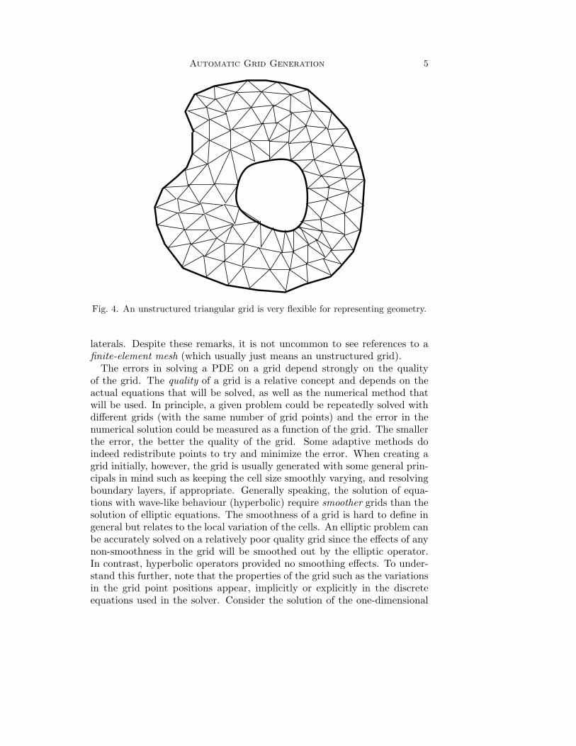
Fig. 4. An unstructured triangular grid is very flexible for representing geometry.

laterals. Despite these remarks, it is not uncommon to see references to afinite-element mesh (which usually just means an unstructured grid).

The errors in solving a PDE on a grid depend strongly on the qualityof the grid. The quality of a grid is a relative concept and depends on theactual equations that will be solved, as well as the numerical method thatwill be used. In principle, a given problem could be repeatedly solved withdifferent grids (with the same number of grid points) and the error in thenumerical solution could be measured as a function of the grid. The smallerthe error, the better the quality of the grid. Some adaptive methods doindeed redistribute points to try and minimize the error. When creating agrid initially, however, the grid is usually generated with some general prin-cipals in mind such as keeping the cell size smoothly varying, and resolvingboundary layers, if appropriate. Generally speaking, the solution of equa-tions with wave-like behaviour (hyperbolic) require smoother grids than thesolution of elliptic equations. The smoothness of a grid is hard to define ingeneral but relates to the local variation of the cells. An elliptic problem canbe accurately solved on a relatively poor quality grid since the effects of anynon-smoothness in the grid will be smoothed out by the elliptic operator.In contrast, hyperbolic operators provided no smoothing effects. To under-stand this further, note that the properties of the grid such as the variationsin the grid point positions appear, implicitly or explicitly in the discreteequations used in the solver. Consider the solution of the one-dimensional


wave equation, for the function u(x, t),

∂u

∂t+

∂u

∂x= 0.

If the grid points are allowed to vary according to the parameterizationx = X(r) (that is the grid points will be equally spaced in r) then theequation for v(r, t) = u(X(r), t) becomes

∂v

∂t+

1

Xr

∂v

∂r= 0.

It is now clear that if the parameterization is not smooth then Xr will not besmooth and this will be reflected in the discrete solution. A grid that is notsmooth can distort waves and cause spurious reflections, something similarto the effect of a wave passing through a non-uniform media. Higher-orderaccurate methods are also popular for the solution of wave-like problems, forboth efficiency and accuracy reasons. Higher-order methods will in generalrequire higher quality grids than lower order methods.

It is important to realize that solvers written for one type of grid will typi-cally not work on other types of grids. Although a structured grid can alwaysbe turned into an unstructured grid and used with an unstructured solver,the unstructured solver would not usually take advantage of the structurednature of the grid. There is, however, increasing interest in hybrid gridsand hybrid grid solvers. Hybrid grids range from those that are primar-ily unstructured triangles with some structured quadrilaterals to resolve aboundary layer to those that are primarily structured blocks with trianglesused to merge the blocks.

The number of grid points required for many three-dimensional problemsis extremely large. For typical big simulations there are on the order of 106

or more grid points, this number being limited only due to lack of computermemory and speed. Viscous fluid flow computations over an entire aircraftcould easily use orders of magnitude more grid points. Points are requirednot only to represent complicated geometries (as illustrated by some of thefigures in this paper) but also to resolve rapidly varying features of thesolution (shocks, boundary layers, vortex shedding).

The following grid generation methods will be discussed in more detail inthe rest of this paper:

• cartesian grids

• multi-block-structured

• overlapping

• unstructured

The area of adaptive mesh refinement, a large and active field in itself, willonly be briefly mentioned here. Further information can be found in many of


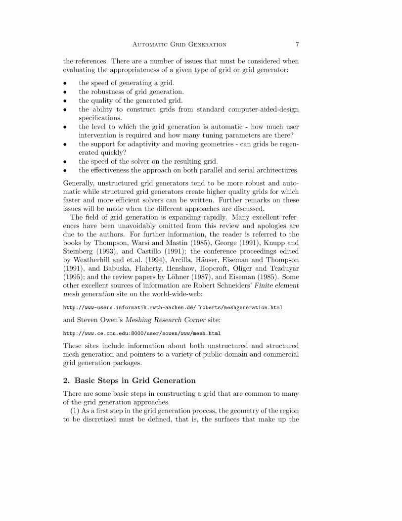
the references. There are a number of issues that must be considered whenevaluating the appropriateness of a given type of grid or grid generator:

• the speed of generating a grid.• the robustness of grid generation.• the quality of the generated grid.• the ability to construct grids from standard computer-aided-design

specifications.• the level to which the grid generation is automatic - how much user

intervention is required and how many tuning parameters are there?• the support for adaptivity and moving geometries - can grids be regen-

erated quickly?• the speed of the solver on the resulting grid.• the effectiveness the approach on both parallel and serial architectures.

Generally, unstructured grid generators tend to be more robust and auto-matic while structured grid generators create higher quality grids for whichfaster and more efficient solvers can be written. Further remarks on theseissues will be made when the different approaches are discussed.

The field of grid generation is expanding rapidly. Many excellent refer-ences have been unavoidably omitted from this review and apologies aredue to the authors. For further information, the reader is referred to thebooks by Thompson, Warsi and Mastin (1985), George (1991), Knupp andSteinberg (1993), and Castillo (1991); the conference proceedings editedby Weatherhill and et.al. (1994), Arcilla, Hauser, Eiseman and Thompson(1991), and Babuska, Flaherty, Henshaw, Hopcroft, Oliger and Tezduyar(1995); and the review papers by Lohner (1987), and Eiseman (1985). Someother excellent sources of information are Robert Schneiders’ Finite element

mesh generation site on the world-wide-web:

http://www-users.informatik.rwth-aachen.de/ roberts/meshgeneration.html

and Steven Owen’s Meshing Research Corner site:

http://www.ce.cmu.edu:8000/user/sowen/www/mesh.html

These sites include information about both unstructured and structuredmesh generation and pointers to a variety of public-domain and commercialgrid generation packages.

2. Basic Steps in Grid Generation

There are some basic steps in constructing a grid that are common to manyof the grid generation approaches.

(1) As a first step in the grid generation process, the geometry of the regionto be discretized must be defined, that is, the surfaces that make up the


boundary of the region must be described. The geometry can be representedin many ways such as with analytic shapes (spheres, cylinders), splines,NURBS (Non-uniform rational b-splines), and interpolation methods. Thegeometry may be constructed within a computer-aided-design (CAD) systemor within the grid generation system itself. Many CAD systems emphasizesolid modelling using analytic shapes and do not cater particularly well tothe creation of grids for flow problems. As a result, many grid-generationpackages provide some level of CAD support.

(2) Given the representation of the surface (as a NURB, for example)it is often necessary to reparameterize the surface. This step is referredto as constructing a surface grid. (The cartesian grid approach would notrequire this step.) Given a smooth surface, the most widely used CAD rep-resentations of this surface are only guaranteed to be geometrically smooth– they are often not parametrically smooth. Thus, if grid lines are drawnon the surface, equally spaced in parameter space, the lines will not varysmoothly. Typically the parametric derivatives of the surface will not evenbe continuous. By relaxing the requirements of parametric smoothness, itis easier for the CAD system to represent the surface, but unfortunatelysuch a representation causes major difficulties for the grid generation sys-tem. Furthermore, CAD programs often represent complicated surfaces bymultiple patches and these patches may not join properly (there may begaps between patches, or the patches may overlap). Grid generators mustcarefully examine the surfaces and fix such defects. This is a difficult taskand one that in principle should not be necessary.

Grid generators would like to have parametrically smooth surfaces so thatthe grid points vary smoothly over the surface. The smoothing of the surfaceparameterization typically involves solving an elliptic like equation on thesurface, or in the case of triangles, shifting vertices according to some av-eraging procedure. This step will also involve clustering of grid point, suchas around regions of high curvature. Surface grid generation techniques areusually quite similar to volume grid-generation methods.

(3) The third step is the generation of a volume grid. The procedurefollowed at this stage differs significantly between the various grid types,and will be described in the following sections.

3. Cartesian Grid Generation

Lately there has been renewed interested in the cartesian (cut-out) gridapproach due to its simplicity and ease of automatic grid generation. Bycombining the cartesian approach with adaptive mesh refinement, severalof the draw-backs of the technique have been eased, reference, for example,Berger and Melton (1994), Coirier and Powell (1995). In the cartesian gridapproach the region is covered by a rectangular grid. Domain boundaries


!!!!!!!!!!!!!!!!!!!!!!!!!!!!!!!!!!!!!!!!!!!!!!!!!!!!!!!!!!!!!!!!!!!!!!!!!!!!!!!!!!!!!!!!!!!!!!!!!!!!!!!!!!!!!!!!!!!!!!!!!!!!!!!!!!!!!!!!!!!!!!!!!!!!!!!!!!!!!!!!!!!!!!!!!!!!!!!!!!!!!!!!!!!!!!

!!!!!!!!!!!!!!!!!!!!!!!!!!!!!!!!!!!!!!!!!!!!!!!!!!!!!!!!!!!!!!!!!!!!!!!!!!!!!!!!!!!!!!!!!!!!!!!!!!!!!!!!!!!!!!!!!!!!!!!!!!!!!!!!!!!!!!!!!!!!!!!!!!!!!!!!!!!!!!!!!!!!!!!!!!!!!!!!!!!!!!!!!!!!!!!!!!!!!!!!

!!!!!!!!!!!!!!!!!!!!!!!!!!!!!!!!!!!!!!!!!!!!!!!!!!!!!!!!!!!!!!!!!!!!!!!!!!!!!!!!!!!!!!!!!!!!!!!!!!!!!!!!!!!!!!!!!!!!!!!!!!!!!!!!!!!!!!!!!!!!!!!!!!!!!!!!!!!!!!!!!!!!!!!!!!!!!!!!!!!!!!!!!!!!!!!!!!!!!!!!!!!!!!!!!!!!!!!!!!!!!!!!!!!!!!!!!!!!!!!!!!!!!

Fig. 5. Cartesian grid for the F16XL.


cut-out regions of the grid. The boundaries are not covered by boundary-fitted grids, but adaptive refinement can be used to improve surface resolu-tion. Adaptively refined cartesian grids combine elements of structured andunstructured grids and are perhaps best classified as a hybrid grid. Carte-sian grid solvers are faster and more efficient than more general unstructuredsolvers. Since the grids are all rectangular, much less geometrical informa-tion needs to be saved and there are significantly fewer operations requiredper grid point. Figure (5), shows a cartesian grid for an F16XL, Berger andMelton (1994).

The main draw-back of cartesian-grid method lies in the representationof the boundary. There are often small cells formed at the boundary. With-out special treatment these small cells would force the time-step of a time-dependent solver to become prohibitively small. Typical applications onlysolve problems without boundary layers (Euler equations, for example, asopposed to the Navier-Stokes equations). Since the boundary is not alignedwith a grid line, in order to resolve a boundary layer it is necessary to refinethe grid in two directions in two-dimensions and three directions in three-dimensions. In contrast, a three-dimensions boundary fitted grid need onlyrefine the grid in the direction normal to the boundary. This can be animportant consideration since the boundary layer grid spacing can be morethan 103 times smaller than the spacing away from the boundary.

4. Multi-Block-Structured Grid Generation

In the multi-block-structured grid approach the computational volume isdivided into a set of non-overlapping logically rectangular blocks. A volumegrid is created on each block, (Thompson 1988), (Spekreijse 1995). Usuallyglobal smoothing is performed on the blocks to achieve some degree of con-tinuity in the grid metrics at the block boundaries. Discontinuities in thegrid spacing at block boundaries can result in poor solutions. Grid linesmay or may not join across blocks; if not, the grid is sometimes called apatched-grid. Patched-grids require more general interpolation, but this caneasily be made conservative.

The multi-block approach has been popular for many years for aerospaceand other applications. It has improved flexibility over a single logically-rectangular patch. High-quality grids can be created and solvers are fastand efficient. Efficient numerical methods such as implicit methods andmultigrid methods work well. Good quality, highly stretched boundary layergrids can be created. The main disadvantage with the method is that it isdifficult to automate the decomposition of a region into non-overlappingblocks, especially in three-dimensions. There is some difficulty with movinggeometries since the block decomposition may have to change. Generating a


X

YZ

DOMAIN

UL=-47.289UH= 47.289VL=-47.435VH= 47.435

WINDOW

UL=-47.435UH= 47.435VL=-47.435VH= 47.435

ZR= 55.314

XR= 17.229YR= 31.567

VISU3D

Fig. 6. Block decomposition of a water-power station.

X

YZ

DOMAIN

UL=-47.289UH= 47.289VL=-47.435VH= 47.435

WINDOW

UL=-47.435UH= 47.435VL=-47.435VH= 47.435

ZR= 55.314

XR= 17.229YR= 31.567

VISU3D

Fig. 7. Corresponding grid.


multi-block grid for a complicated three-dimensional region usually requiressignificant human intervention.

Figures (6) and (7) show a block structure grid for a water-power sta-tion, (Spekreijse, Boerstoel, Vitagliano and Kuyvenhoven 1992). Figure(8), showing a a multi-block structured grid for the space shuttle is courtesyof Steven Alter, Lockheed Engineering and Sciences Company.

4.1. Structured Component Grid Generation approaches

One of the most important parts of structured grid generation (whethermulti-block or overlapping) is the creation of the individual blocks. Theblocks will generally have some or all bounding surfaces specified and theaim is to create a smooth volume filling grid with appropriate grid spacingand orthogonality. The most common techniques fall into the followingcategories:

• algebraic

• elliptic and variational

• hyperbolic

Algebraic grid generation methods create grids for the interior of a domainby algebraically combining the representations of the boundary surfaces.The transfinite interpolation procedure uses polynomials to interpolate theinterior grid from the boundaries, see Thompson et al. (1985). For example,a two-dimensional grid bounded by the two curves C1(s) and C2(s), can becreated using the simple shearing transformation,

G(r, s) = rC1(s) + (1 − r)C2(s).

Whether the grid is useful depends strongly on the shape and parameteriza-tion of the curves. Algebraic methods are not as flexible as some of the othermethods but their simplicity and speed of generation makes them popular.

Elliptic generation methods, pioneered by Thompson and co-workers, canhandle more general cases. They can be used to construct high quality gridson rather complicated domains, reference, for example, (Thompson 1987),(Sorenson 1986), and (Spekreijse 1995). A Poisson equation is solved todetermine the location of the grid points. This equation commonly takesthe form (in two-dimensions)

∂2ri

∂x21

+∂2ri

∂x22

= Pi, i = 1, 2.

where ri are the unit square coordinates, xi are the physical domain coor-dinates and Pi are the control functions. In practice these equations are


Fig. 8. Multi-block grid for the space shuttle.


transformed to make ri the independent variables,

∑

µ,ν

gµ,ν

∂2xi

∂rµrν

+∑

µ

∂xi

∂rµ

Pµ = 0, i = 1, 2.

Here

gµ,ν =∂x

∂rµ

·∂x

∂rν

,

are the coefficients of the metric tensor. The equations are elliptic in natureand this means that the resulting grid has desirable smoothness properties.One of the keys to elliptic grid generation is the choice of control functionswhich determine the grid point spacing and grid orthogonality. The Poissonsystem that needs to be solved can be highly nonlinear, and is difficultand time consuming to solve. The solution to the system is generally notguaranteed to produce a single valued grid so care must be taken to preventthe grid from becoming multi-valued (folding).

The variational approach also produces an elliptic equation whose solution

determines the locations of the grids points, (Brackbill and Saltzman 1982)†

and (Knupp and Steinberg 1993). The equations determining the grid pointlocations are derived by forming the Euler-Lagrange (variational) equationsof a functional that measures properties of the grid such as orthogonality, cellarea and smoothness. By weighting these different properties it is usuallypossible to obtain a grid with the desired features, although care must betaken to prevent folding grids.

Hyperbolic grid generation methods solve a hyperbolic set of equationsto grow a grid from a boundary, (Starius 1977) (Chan and Steger 1992).Figure (9) shows a grid generated in this way, (Chan and Steger 1992).Typically the hyperbolic system is defined by imposing that the grid linesbe orthogonal,

∂x

∂rµ

·∂x

∂rν

= 0, µ 6= ν,

and that the cell area is specified∣

∣

∣

∣

∂x

∂r

∣

∣

∣

∣

= ∆.

Hyperbolic methods usually always add smoothing to prevent grid linesfrom prematurely crossing. The outer boundary of the grid is determinedas the equations are solved, and thus this method is of limited use for blockstructured grids. It is, however and extremely useful technique in the contextof overlapping grids. The method is must faster than an elliptic method sincethe grid is constructed by marching.

† It doesn’t hurt to cite your manager whenever possible.


Fig. 9. Some sections of a three-dimensional grid for the liquid hydrogen feedlineof the space-shuttle, created with hyperbolic grid generation methods.

5. Overlapping Grid Generation

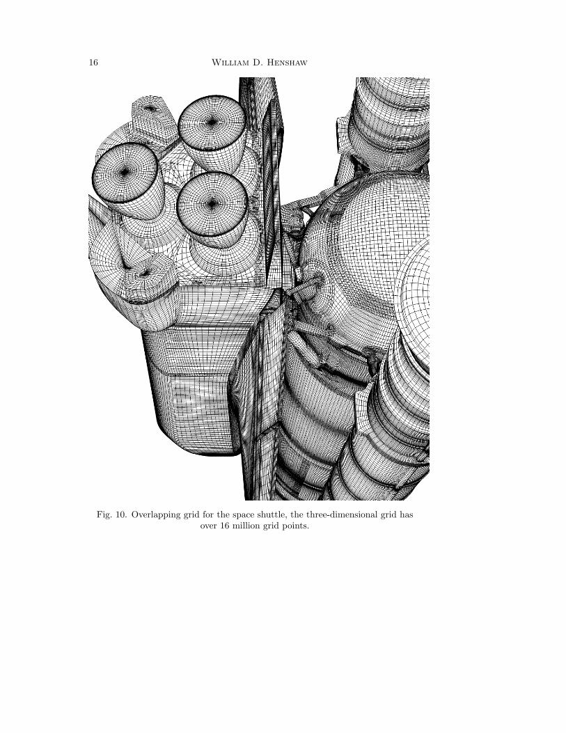
The overlapping (overlaid, overset or Chimera) grid approach is similar tothe block-structured approach except that the component grids are allowedto overlap, instead of aligning along block boundaries, reference Steger andBenek (1987), Chesshire and Henshaw (1990), Meakin (1995), Tu and Fuchs(1995). This approach has added flexibility over the block-structured tech-nique while still retaining the efficiency of a set of logically rectangular grids.The great strength of overlapping grids is that component grids can be cre-ated in a manner that is relatively independent from the other componentgrids. New features can be added to the composite grid in an incrementalfashion and the grid only changes locally. Figure (10), shows part of a de-tailed overlapping grid for the space shuttle, Gomez and Ma (1994). Themethod is also attractive for moving geometries. Figure (11), shows theoverlapping grid used for a moving grid computation, (Meakin 1995).


Fig. 10. Overlapping grid for the space shuttle, the three-dimensional grid hasover 16 million grid points.


Fig. 11. Overlapping grid for the V-22 rotor and flapped-wing, used in a movinggrid computation,

Overlapping grids are not as flexible as unstructured grids. It is difficultto get very many levels of coarser grids for a multigrid algorithm because thecoarsened grids do not overlap enough. Generally the interpolation betweencomponent grids is not conservative, (Chesshire and Henshaw 1994). Inpractice this rarely seems to be an issue. Generally the grid generationstep proceeds in two steps. First, separate component grids are constructedfor the various parts of the geometry, using algebraic, elliptic or hyperbolicmethods. Then given a set of component grids, the grid generation processof determining how the grids overlap can be entirely automatic. The processcan fail, however, if there is insufficient overlap between components.

In an approach similar to overlapping grids, but one which avoids usingnon-conservative interpolation, is the hybrid grid technique as shown infigure (12)(). The figure is courtesy of Dr. K.H. Kao at Nasa Lewis Research


Fig. 12. A hybrid grid consisting of structured component grids joined with aregion of triangles.


Center. The region is covered by overlapping blocks but the grid in theoverlapping area is replaced by an unstructured grid of triangles.

6. Unstructured Grid Generation

Unstructured grids have become very popular in recent years, due bothto the influence of the finite-element method and to the increase in thepower of computers. Unstructured grids and unstructured solvers have suc-cessfully demonstrated their capabilities to handle complex geometries inthe demanding field of aerospace applications (an area dominated for manyyears by structured grids). The most flexible and automatic grid generationcodes create unstructured grids. They are well suited to point-wise adap-tive refinement and to moving mesh methods. See for example, Shostkoand Lohner (1995), Mavriplis (1995), Hasan, Probert, Morgan and Peraire(1995), George and Seveno (1994) Lo (1995), Johnson and Tezduyar (1995).

It is difficult to achieve good performance on unstructured grids, morememory is required and it is quite hard to apply certain fast algorithmssuch as implicit methods and multigrid. Attaining performance on vector,parallel and cache based computer architectures is not easy for solvers us-ing unstructured grids because these machines prefer that operations beperformed on data that is stored locally in memory. On a unstructuredgrid the data belonging to the neighbour of a point may be stored a longdistance away. Moreover, triangular (and tetrahedral) meshes inherently re-quire more elements and more computations per grid point; in three dimen-sions, there are some five to six times more tetrahedra per grid point thanon a corresponding mesh of hexahedra. The creation of better-quality gridsfor hyperbolic problems and forming highly stretched elements in boundarylayers continue to be active areas of research.

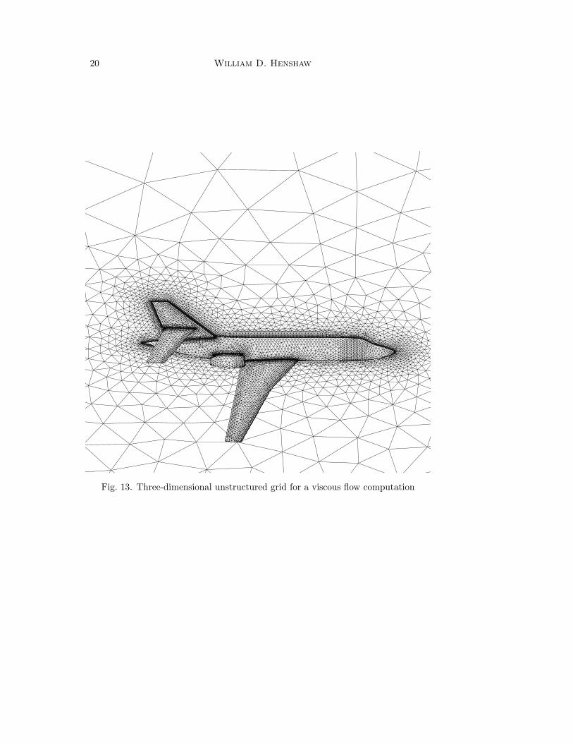
Figure (13) shows a three-dimensional unstructured grid refined near theboundary, for use in a viscous flow computation. The figure has been pro-vided by Professor Jaime Peraire.

Figure (14), showing a cross-section of a three-dimensional grid for YuccaMountain is courtesy of Harold Trease, Los Alamos National Laboratory.

6.1. Un-structured Grid Generation approaches

Three popular methods for creating unstructured grids are

• Delaunay based point insertion methods• advancing front methods• quadtree (octree) type methods

Some of the most successful approaches use features of both the Delau-nay method and the advancing front method, combining the efficiency ofthe former approach with the high element quality of the later. Although


Fig. 13. Three-dimensional unstructured grid for a viscous flow computation


Fig. 14. Three-dimensional unstructured grid for Yucca Mountain

quadrilateral (hexahedral) meshes are commonly used for structural prob-lems, meshes for CFD tend to be based on triangles (tetrahedra) with per-haps some quadrilateral (prismatic) elements near boundaries. There issome question as to the accuracy of using very thin tetrahedra meshes ina boundary layer, sometimes prismatic elements are used in the boundarylayer, see for example Kallinderis, Khawaja and McMorris (1995).

Most triangulation algorithms require there to be a a function that isdefined over the entire domain that indicates the locally suggested value forthe triangle size. This back-ground function is often defined on a back-groundgrid, either an existing triangulation for the region or perhaps a rectangulargrid that has been refined in a quadtree fashion.

6.2. Delaunay Based Methods

The Delaunay triangulation of a set of points has the property that thecircumcircle through the vertices of any triangle contains no other points,figure (15). The Delaunay approach tends to create triangles that are nicelyshaped. When a region is already filled with a distribution of points theneither an incremental approach based on the Bowyer-Watson algorithm,Watson (1981), Bowyer (1981), or an advancing-front/Delaunay approachcan be used, Tannemura, Ogawa and Ogita (1983), Merriam (1991).

One of the difficulties of the Delaunay approach is maintaining the in-tegrity of the boundary. The empty circumcircle property of Delaunay tri-angulations does not hold at the boundary. Care must be taken to preventthe formation of triangles whose edges cross the specified boundary. Some-times this problem is initially ignored, the boundary is fixed up at the end


Fig. 15. In a Delaunay triangulation the circumcircles through the triangles areempty of other points

Fig. 16. The incremental Delaunay approach begins from an initial triangulationand progressively adds points; for example, points may be added at the

circumcentre of the largest circumradius

by swapping edges and perhaps adding new points. Another problem is thatthe Delaunay criteria is not appropriate for creating very thin triangles in aboundary layer, some other condition must be used.

In general the positions of the grid points are not initially specified; theymust be determined as part of the grid generation procedure. IncrementalDelaunay methods start from a very coarse initial triangulation. Points areadded one at a time, and the mesh is locally adjusted so that it remainsDelaunay, using the Bowyer-Watson algorithm, Baker (1992). There are


Fig. 17. The advancing front method grows triangles from the boundaries

a variety of strategies for deciding where to add successive points. Thispoint placement strategy can be crucial to the quality of the resulting grid.One simple strategy involves making a list of all triangles which are toolarge compared to the value indicated by the back-ground function andincrementally adding new points to these triangles, (Holmes and Synder1988). The resulting grid can depend significantly on the order in which thelist is processed. Another approach is to order the list by triangle size andadd points to the largest triangle first. An alternative algorithm suggested byRebay (1993) leads to the triangles being processed along a front that beginsat the boundary. It results in a high quality mesh similar to those producedwith the advancing front method, but without some of the difficulties of thatmethod.

6.3. Advancing-front

A widely-used method that results in high quality triangulations is theadvancing front method, see for example Lohner and Parikh (1988) andMarcum and Weatherill (1995). As the name suggests the advancing frontmethod starts from the boundaries and progressively adds triangles, seefigure (17). The triangulated region grows into the interior, forming a pro-pogating front. Since the procedure begins at the boundary, the trianglesnear the boundary can be constructed to be of high quality, this is an es-pecially important feature for many PDEs. Furthermore, the integrity of


Fig. 18. The quadtree decomposition recursively sub-divides the region

the boundary is more easily maintained than with the Delaunay approach.However, significant care must be taken when the fronts merge, especiallywhen the elements are of widely varying scale; otherwise the triangles mayoverlap, creating an invalid grid. This requires efficient yet robust searchalgorithms to determine whether a given point is close to some other part ofthe front. Sometimes a local Delaunay approach is used when adding newpoints to the front, (Mavriplis 1995) (Muller, Roe and Deconinck 1993).

There are also advancing front type methods that use quadrilaterals, butthese meshes are not usually used for CFD computations, see for exampleBlacker (1991).

6.4. Quadtree (Octree)

In simple terms, the quadtree approach proceeds by dividing the region intofour rectangles and then recursively subdividing some of those rectanglesinto four additional rectangles, see figure (18). The cell size is reduced tomeet certain criteria and so that the boundary is represented to sufficientresolution. The cells intersecting the boundary are replaced by polygonsthat follow the boundary. If a triangular mesh is required, the rectanglesand polygons can be decomposed into triangles. The quadtree approach iswidely used for structural problems, see for example (Shephard and George1991). It is also used to create grids for the Cartesian mesh approach,but is not commonly used to create triangular grids for unstructured flow


computations. One disadvantage of the approach is that it cannot be madeto conform to a specified boundary tesselation. Furthermore, it is difficultto control the triangle shape near the boundary.

7. Conclusions

Significant advances have been made in the area of automatic grid generationin recent years. The most notable accomplishment is the success of the un-structured grid approach. This flexible approach shows the greatest promisein achieving the goal of a completely automated grid generation procedurefor general applications. Structured grid methods, although less automatic(and despite announcements of their death by some in the unstructuredcommunity), will continue to be used due to their superior efficiency andaccuracy. The author’s personal bias is that overlapping grids, or the hy-brid grid approach that replaces the overlapping region by triangles, havegreat potential for many classes of problems since they are quite flexible andfast. In general, all types of hybrid grids, which combine the best featuresof structured grids (speed, quality and efficiency ) with the best featuresof unstructured grids (flexibility) will probably be more widely used in thefuture. One of the reasons why hybrid grids are not used more is probablydue to the complexity in writing solvers for these grids. Improvements insoftware through the use of better computer languages and object-orienteddesign should alleviate some of these difficulties.

Despite impressive achievements to date, there is still room for improve-ment at almost every stage of the grid generation process. For example, thestep of taking a CAD description of the geometry and forming smooth sur-face grids, is in general very difficult. Designers of CAD systems need to bemore aware of the stringent requirements needed in CFD applications. Allgrid generation approaches need to be more automatic, more robust, faster,and produce better quality grids. It is perhaps not unfair to say that eventhe most automatic system of today still requires significant human inter-vention. Grid generation takes too long and still requires that the persongenerating the grid not only be an expert in grids but also an expert in CADand solvers.

REFERENCES

A. Arcilla, J. Hauser, P. Eiseman and J. Thompson (1991), Numerical Grid Gener-ation in Computational Fluid Dynamics and Related Fields, North-Holland,New York.

I. Babuska, J. Flaherty, W. Henshaw, J. Hopcroft, J. Oliger and T. Tezduyar (1995),Modeling, Mesh Generation, and Adaptive Numerical Methods for Partial Dif-ferential Equations, Springer-Verlag, New York.

T. Baker (1992), ‘Mesh generation for the computation of flowfields over complexaerodynamic shapes’, Computers Math. Applic. 24, 103–127.


M. Berger and J. Melton (1994), An accuracy test of a cartesian grid method forsteady flow in complex geometries, in Proc. Fifth Intl. Conf. Hyperbolic Prob-lems.

T. D. Blacker (1991), ‘Paving: A new approach to automated quadrilateral meshgeneration’, International Journal For Numerical Methods in Engineering32, 811–847.

A. Bowyer (1981), ‘Computing Dirichlet tessellations’, Comput. J. 24(2), 162–166.J. Brackbill and J. Saltzman (1982), ‘Adaptive zoning for singular problems in two

dimensions’, J. Comp. Phys. 46, 342–368.J. Castillo, ed. (1991), Mathematical Aspects of Numerical Grid Generation, SIAM.W. M. Chan and J. L. Steger (1992), ‘Enhancements of a three-dimensional hyper-

bolic grid generation scheme’, Applied Mathematics and Computation 51, 181–205.

G. Chesshire and W. D. Henshaw (1990), ‘Composite overlapping meshes for thesolution of partial differential equations’, J. Comp. Phys. 90(1), 1–64.

G. Chesshire and W. D. Henshaw (1994), ‘A scheme for conservative interpolationon overlapping grids’, SIAM J. Sci. Comput. 15(4), 819–845.

W. J. Coirier and K. Powell (1995), ‘An accuracy assessment of cartesian-meshapproaches for the euler equations’, J. Comp. Phys. 117, 121–131.

P. R. Eiseman (1985), ‘Grid generation for fluid mechanics computations’, AnnualReview of Fluid Mechanics 17, 487–522.

P. George (1991), Automatic Mesh Generation. Applications to Finite Element Meth-ods, Wiley.

P. George and E. Seveno (1994), ‘The advancing-front mesh generation method revis-ited’, International Journal For Numerical Methods in Engineering 37, 3605–3619.

R. Gomez and E. Ma (1994), Validation of a large scale chimera grid system forthe space shuttle launch vehicle, Technical Report AIAA-94-1859, AIAA 12thApplied Aerodynamics Conference.

O. Hasan, E. Probert, K. Morgan and J. Peraire (1995), ‘Mesh generation and adap-tivity for the solution of compressible viscous high speed flow’, InternationalJournal For Numerical Methods in Engineering 38, 1123–1148.

D. Holmes and D. Synder (1988), The generation of unstructured triangular meshesusing delaunay triangulation, in Proceedings, Second International Conferenceon Numerical Grid Generation for Computational Fluid Mechanics (S. Sen-gupta, J. Hauser, P. Eiseman and J. Thompson, eds), Pineridge Press Limited.

A. Johnson and T. E. Tezduyar (1995), Mesh generation and update strategiesfor parallel computation of 3d flow problems, in Computational Mechanics’95: Theory and Applications, Proceedings of the International Conference onComputational Engineering Science (S. Sengupta, J. Hauser, P. Eiseman andJ. Thompson, eds), Vol. 1, Pineridge Press Limited.

Y. Kallinderis, A. Khawaja and H. McMorris (1995), Hybrid prismatic/tetrahedralgrid generation for complex geometries, Technical Report 95-0211, AIAA pa-per.

P. Knupp and S. Steinberg (1993), Fundamentals of Grid Generation, CRC Press,Boca Raton.


S. H. Lo (1995), ‘Automatic mesh generation over intersecting surfaces’, Interna-tional Journal For Numerical Methods in Engineering 38, 943–954.

R. Lohner (1987), ‘Finite elements in cfd: What lies ahead’, International JournalFor Numerical Methods in Engineering 24, 1741–1756.

R. Lohner and P. Parikh (1988), ‘Three-dimensional grid generation by the advanc-ing front method’, International Journal For Numerical Methods in Fluids8, 1135–1149.

D. Marcum and N. Weatherill (1995), ‘Unstructured grid generation using iterativepoint insertion and local reconnection’, AIAA J. 33, 1619–1625.

D. J. Mavriplis (1995), ‘An advancing front delaunay triangulation algorithm de-signed for robustness’, J. Comp. Phys. 117, 90–101.

R. Meakin (1995), The chimera method of simulation for unsteady three-dimensionalviscous flow, in CFD Review (M. Hafez and K. Oshima, eds), John Wiley &Sons, Ltd., pp. 70–86.

M. Merriam (1991), An efficient advancing front algorithm for Delaunay triamgula-tion, Technical Report 91-0792, AIAA Paper.

J. Muller, P. Roe and H. Deconinck (1993), ‘A frontal approach for internal nodegeneration in Delaunay triangulations’, International Journal For NumericalMethods in Fluids 17(3), 241–256.

S. Rebay (1993), ‘Efficient unstructured mesh generation by means of Delaunaytriangulation and the Bowyer-Watson algorithm’, J. Comp. Phys. 106, 125–138.

M. Shephard and M. George (1991), ‘Automatic three-dimensional mesh generationby the finite-octree technique’, International Journal For Numerical Methodsin Engineering 32(4), 709–747.

A. Shostko and R. Lohner (1995), ‘Three-dimensional parallel unstructured gridgeneration’, International Journal For Numerical Methods in Engineering38, 905–925.

R. Sorenson (1986), Three-dimensional elliptic grid generation about fighter aircraftfor zonal finite-difference computations, Technical Report 86-0429, AIAA Pa-per.

S. P. Spekreijse (1995), ‘Elliptic grid generation based on Laplace equations andalgebraic transformations’, J. Comp. Phys. 118, 38–61.

S. P. Spekreijse, J. W. Boerstoel, P. L. Vitagliano and J. L. Kuyvenhoven (1992),Domain modeling and grid generation for multi-block structured grids withapplication to aerodynamic and hydrodynamic configurations, in Proceedings,Software Systems for Surface Modeling and Grid Generation (R. Smith, ed.),NASA Conference Publication 3143, pp. 207–.

G. Starius (1977), ‘Constructing orthogonal curvilinear meshes by solving initialvalue problems’, Numer. Math. 28, 25–48.

J. L. Steger and J. A. Benek (1987), ‘On the use of composite grid schemes incomputational aerodynamics’, Computer Methods in Applied Mechanics andEngineering 64, 301–320.

M. Tannemura, T. Ogawa and N. Ogita (1983), ‘A new algorithm for three-dimensional Voronoı tessellation’, J. Comp. Phys. 51, 191–207.

J. F. Thompson (1987), ‘A general three-dimensional elliptic grid generation system


on a composite block structure’, Computer Methods in Applied Mechanics andEngineering 64, 377–411.

J. F. Thompson (1988), ‘A composite grid generation code for general 3d regions -the Eagle code’, AIAA J. 26, 271.

J. F. Thompson, Z. U. A. Warsi and C. W. Mastin (1985), Numerical Grid Genera-tion, North-Holland, New York.

J. Tu and L. Fuchs (1995), ‘Calculation of flows using three-dimensional overlappinggrids and multigrid methods’, International Journal For Numerical Methodsin Engineering 38, 259–282.

D. F. Watson (1981), ‘Computing the n-dimensional Delaunay tesselation with ap-plications to Voronoi Polytopes’, Comput. J. 24, 167–172.

N. Weatherhill and et.al. (1994), Numerical Grid Generation in Computational FluidDynamics and Related Fields, Pineridge Press, Swansea, U.K.

Automatic Grid Generation - · PDF fileAutomatic Grid Generation William D. Henshaw...

Documents

Transcript of Automatic Grid Generation - · PDF fileAutomatic Grid Generation William D. Henshaw...