Automated Segmentation and Pathology Detection in Ophthalmic ...

Automated Segmentation and Pathology Detection inOphthalmic Images

A DISSERTATION

SUBMITTED TO THE FACULTY OF THE GRADUATE SCHOOL

OF THE UNIVERSITY OF MINNESOTA

BY

Sohini Roy Chowdhury

IN PARTIAL FULFILLMENT OF THE REQUIREMENTS

FOR THE DEGREE OF

Doctor of Philosophy

Professor Keshab K. Parhi, Advisor; Dr. Dara D. Koozekanani, Co-advisor

July, 2014

c© Sohini Roy Chowdhury 2014

ALL RIGHTS RESERVED

Acknowledgements

First of all, I would like to thank my advisor Professor Keshab K. Parhi for his continued

guidance, support and encouragement for my work. I also would like to thank my co-

advisor Dr. Dara D. Koozekanani for his constant guidance and inputs that helped me

hone my skills of retinal image processing.

I would like to thank Professor Mostafa Kaveh and Professor Jarvis Haupt for their

support as members of my Ph.D. committee. I would like to thank Dr. Salma Radwan,

Dr. Sam Kuchinka and Dr. Michael Reinsbach for providing manually annotated data

sets and helping me understand retinal image diagnostics. I would like to thank the

Graduate School, the Department of Electrical and Computer Engineering and The

Department of Ophthalmology and Vision Neurosciences at the University of Minnesota

for their financial support.

I would like to thank my parents, my brother, sister-in-law and little nephew for

their love and unwavering support through my trying times. I want to thank my fiance

and in-laws for their unquestioned affection and constant inspiration for perfection.

I want to thank my lab mates Bo Yuan, Tingting Xu, Manohar Ayinala, Shu-

Hsein Chu, Yin Liu, Yingjie Lao, Zisheng Zhang and Chuan Zhang for their friendship,

enlightening talks about research and the future ahead.

Last, but not the least, I want to thank my friends Ayan Paul, Rajasree Roy Burman,

Shubharajit Roychowdhury, Sanjoy Dey for their friendship and kindness. I want to

thank Somnath Kundu for the many long walks across Minneapolis and for being such

a worthy accomplice as graduate school munchies. I want to thank Lucy Marie, Joseph

Bennett and little Jonah Reed Bennett for cheering me up at all moments, especially

when it meant the most.

i

Abstract

Computer-aided medical diagnostic system design is an emerging inter-disciplinary tech-

nology that assists medical practitioners for providing quick and accurate diagnosis and

prognosis of pathology. Since manual assessments of digital medical images can be both

ambiguous and time-consuming, computer-aided image analysis and evaluation systems

can be beneficial for baseline diagnosis, screening and disease prioritization tasks. This

thesis presents automated algorithms for detecting ophthalmic pathologies pertaining

to the human retina that may lead to acquired blindness in the absence of timely di-

agnosis and treatment. Multi-modal automated segmentation and detection algorithms

for diabetic manifestations such as Diabetic Retinopathy and Diabetic Macular Edema

are presented. Also, segmentation algorithms are presented that can be useful for au-

tomated detection of Glaucoma, Macular Degeneration and Vein Occlusions. These

algorithms are robust to normal and pathological images and incur low computation-

ally complexity.

First, we present a novel blood vessel segmentation algorithm using fundus images

that extracts the major blood vessels by applying high-pass filtering and morphological

transforms followed by addition of fine vessel pixels that are classified by a Gaussian

Mixture Model (GMM) classifier. The proposed algorithm achieves more than 95%

vessel segmentation accuracy on three publicly available data sets. Next, we present an

iterative blood vessel segmentation algorithm that initially estimates the major blood

vessels, followed by iterative addition of fine blood vessel segments till a novel stopping

criterion terminates the iterative vessel addition process. This iterative algorithm is

specifically robust to thresholds since it achieves 95.35% vessel segmentation accuracy

with 0.9638 area under ROC curve (AUC) on abnormal retinal images from the publicly

available STARE data set.

We propose a novel rule-based automated optic disc (OD) segmentation algorithm

that detects the OD boundary and the location of vessel origin (VO) pixel. This al-

gorithm initially detects OD candidate regions at the intersection of the bright regions

and the blood vessels in a fundus image subjected to certain structural constraints, fol-

lowed by the estimation of a best fit ellipse around the convex hull that combines all the

ii

detected OD candidate regions. The centroid of the blood vessels within the segmented

OD boundary is detected as the VO pixel location. The proposed algorithm results in

an average of 80% overlap score on images from five public data sets.

We present a novel computer-aided screening system (DREAM) that analyzes fun-

dus images with varying illumination and fields of view, and generates a severity grade

for non-proliferative diabetic retinopathy (NPDR) using machine learning. Initially, the

blood vessel regions and the OD region are detected and masked as the fundus image

background. Abnormal foreground regions corresponding to bright and red retinopathy

lesions are then detected. A novel two-step hierarchical classification approach is pro-

posed where the non-lesions or false positives are rejected in the first step. In the second

step, the bright lesions are classified as hard exudates and cotton wool spots, and the

red lesions are classified as hemorrhages and micro-aneurysms. Finally, the number of

lesions detected per image is combined to generate a severity grade. The DReAM sys-

tem achieves 100% sensitivity, 53.16% specificity and 0.904 AUC on a publicly available

MESSIDOR data set with 1200 images. Additionally, we propose algorithms that detect

post-operative laser scars and fibrosed tissues and neovascularization in fundus images.

The proposed algorithm achieves 94.74% sensitivity and 92.11% specificity for screen-

ing normal images in the STARE data set from the images with proliferative diabetic

retinopathy (PDR).

Finally, we present a novel automated system that segments six sub-retinal thickness

maps from optical coherence tomography (OCT) image stacks of healthy patients and

patients with diabetic macular edema (DME). First, each image in the OCT stack

is denoised using a Wiener Deconvolution algorithm that estimates the speckle noise

variance using a Fourier-domain based structural error. Next, the denoised images

are subjected to an iterative multi-resolution high-pass filtering algorithm that detects

seven sub-retinal surfaces in six iterative steps. The thicknesses of each sub-retinal

layer for all scans from a particular OCT stack are then combined to generate sub-

retinal thickness maps. Using the proposed system the average inner sub-retinal layer

thickness in abnormal images is estimated as 275µm (r = 0.92) with an average error

of 9.3 µm, while the average thickness of the outer segments in abnormal images is

estimated as 57.4 µm (r = 0.74) with an average error of 3.5 µm. Further analysis of

the thickness maps from abnormal OCT image stacks demonstrates irregular plateau

iii

regions in the inner nuclear layer (INL) and outer nuclear layer (ONL), whose area can

be estimated with r = 0.99 by the proposed segmentation system.

iv

Contents

Acknowledgements i

Abstract ii

List of Tables ix

List of Figures xii

1 Introduction 1

1.1 Introduction . . . . . . . . . . . . . . . . . . . . . . . . . . . . . . . . . . 1

1.2 Summary of Contributions . . . . . . . . . . . . . . . . . . . . . . . . . . 5

1.2.1 Segmentation of Retinal Anatomical Regions in Fundus Images . 5

1.2.2 DR Screening Systems using Funds Images . . . . . . . . . . . . 7

1.2.3 Automated Segmentation of OCT images . . . . . . . . . . . . . 7

1.3 Outline of this Thesis . . . . . . . . . . . . . . . . . . . . . . . . . . . . 7

2 Automated Vessel Segmentation: A Classification Approach 9

2.1 Introduction . . . . . . . . . . . . . . . . . . . . . . . . . . . . . . . . . . 9

2.2 Prior Work . . . . . . . . . . . . . . . . . . . . . . . . . . . . . . . . . . 11

2.3 Method and Materials . . . . . . . . . . . . . . . . . . . . . . . . . . . . 13

2.3.1 Data . . . . . . . . . . . . . . . . . . . . . . . . . . . . . . . . . . 13

2.3.2 Problem Formulation . . . . . . . . . . . . . . . . . . . . . . . . 14

2.3.3 Pixel-based Classification . . . . . . . . . . . . . . . . . . . . . . 17

2.4 Experimental Evaluation and Results . . . . . . . . . . . . . . . . . . . . 22

2.4.1 Vessel Segmentation Performance . . . . . . . . . . . . . . . . . . 24

v

2.4.2 Abnormal Image Analysis . . . . . . . . . . . . . . . . . . . . . . 28

2.4.3 Cross-Training by inter-changing the Training/Test data . . . . . 29

2.4.4 Peripapillary vessel analysis . . . . . . . . . . . . . . . . . . . . . 30

2.5 Discussion and Conclusions . . . . . . . . . . . . . . . . . . . . . . . . . 31

3 Automated Vessel Segmentation: An Iterative Algorithm 40

3.1 Introduction . . . . . . . . . . . . . . . . . . . . . . . . . . . . . . . . . . 40

3.2 Prior Work . . . . . . . . . . . . . . . . . . . . . . . . . . . . . . . . . . 42


3.3.1 Data . . . . . . . . . . . . . . . . . . . . . . . . . . . . . . . . . . 44

3.3.2 Proposed Method . . . . . . . . . . . . . . . . . . . . . . . . . . . 45

3.4 Experimental Evaluation and Results . . . . . . . . . . . . . . . . . . . . 55

3.4.1 Vessel Segmentation Performance . . . . . . . . . . . . . . . . . . 56

3.4.2 Abnormal Image Analysis . . . . . . . . . . . . . . . . . . . . . . 57

3.4.3 Peripapillary vessel analysis . . . . . . . . . . . . . . . . . . . . . 57

3.5 Discussion and Conclusions . . . . . . . . . . . . . . . . . . . . . . . . . 59

4 Automated Optic Disc Segmentation 71

4.1 Introduction . . . . . . . . . . . . . . . . . . . . . . . . . . . . . . . . . . 71

4.2 Overview of Prior Work . . . . . . . . . . . . . . . . . . . . . . . . . . . 73

4.3 Materials and Method . . . . . . . . . . . . . . . . . . . . . . . . . . . . 75

4.3.1 Data . . . . . . . . . . . . . . . . . . . . . . . . . . . . . . . . . . 76

4.3.2 Proposed Method . . . . . . . . . . . . . . . . . . . . . . . . . . . 77

4.4 Results . . . . . . . . . . . . . . . . . . . . . . . . . . . . . . . . . . . . . 82

4.4.1 Metrics . . . . . . . . . . . . . . . . . . . . . . . . . . . . . . . . 82

4.4.2 Segmentation Performance . . . . . . . . . . . . . . . . . . . . . 84

4.4.3 Distribution of Performance metrics . . . . . . . . . . . . . . . . 86

4.5 Conclusions and Discussion . . . . . . . . . . . . . . . . . . . . . . . . . 87

5 Automated Non-Proliferative Diabetic Retinopathy Detection 101

5.1 Introduction . . . . . . . . . . . . . . . . . . . . . . . . . . . . . . . . . . 101


5.2.1 Data . . . . . . . . . . . . . . . . . . . . . . . . . . . . . . . . . . 105

vi

5.2.2 Lesion Classification . . . . . . . . . . . . . . . . . . . . . . . . . 106

5.3 Proposed System . . . . . . . . . . . . . . . . . . . . . . . . . . . . . . . 107

5.3.1 Stage 1: Image Segmentation . . . . . . . . . . . . . . . . . . . . 107

5.3.2 Stage 2: Lesion Classification . . . . . . . . . . . . . . . . . . . . 109

5.3.3 Stage 3: DR Severity Grading . . . . . . . . . . . . . . . . . . . . 113

5.4 Results . . . . . . . . . . . . . . . . . . . . . . . . . . . . . . . . . . . . . 113

5.4.1 Feature Set and Classifier Evaluation for Data Set 1: DIARETDB1114

5.4.2 Classifier Evaluation for Data Set 2: MESSIDOR . . . . . . . . . 116

5.4.3 Time complexity Analysis of the DREAM system . . . . . . . . . 117

5.4.4 Comparison with Prior Work . . . . . . . . . . . . . . . . . . . . 118


6 Automated Proliferative Diabetic Retinopathy Detection 130

6.1 Introduction . . . . . . . . . . . . . . . . . . . . . . . . . . . . . . . . . . 130


6.2.1 Detection of Laser Scars and Fibrosis . . . . . . . . . . . . . . . 135

6.2.2 Detection of NVD . . . . . . . . . . . . . . . . . . . . . . . . . . 136

6.2.3 Detection of NVE . . . . . . . . . . . . . . . . . . . . . . . . . . 138

6.3 Results . . . . . . . . . . . . . . . . . . . . . . . . . . . . . . . . . . . . . 140


7 Automated Segmentation of Optical Coherence Tomography Images 149

7.1 Introduction . . . . . . . . . . . . . . . . . . . . . . . . . . . . . . . . . . 149


7.2.1 Automated Denoising . . . . . . . . . . . . . . . . . . . . . . . . 155

7.2.2 Automated Segmentation . . . . . . . . . . . . . . . . . . . . . . 156

7.2.3 Sub-retinal Layer Thickness Maps . . . . . . . . . . . . . . . . . 158

7.3 Experiments and Results . . . . . . . . . . . . . . . . . . . . . . . . . . . 159

7.3.1 Performance of Automated Denoising . . . . . . . . . . . . . . . 160

7.3.2 Sub-retinal Surface Segmentation Error . . . . . . . . . . . . . . 162

7.3.3 Sub-retinal Layer Thickness Estimation . . . . . . . . . . . . . . 164

7.3.4 Thickness Map Analysis . . . . . . . . . . . . . . . . . . . . . . . 165


vii

8 Conclusions and Future Work 175

8.1 Conclusions . . . . . . . . . . . . . . . . . . . . . . . . . . . . . . . . . . 175

8.1.1 Automated Segmentation of Retinal Anatomical Regions in Fun-

dus Images . . . . . . . . . . . . . . . . . . . . . . . . . . . . . . 175

8.1.2 Automated DR screening systems . . . . . . . . . . . . . . . . . 176

8.1.3 Automated Segmentation of OCT images . . . . . . . . . . . . . 177

8.2 Future Work . . . . . . . . . . . . . . . . . . . . . . . . . . . . . . . . . 177

References 179

viii

List of Tables

2.1 Optimal feature set identified by feature voting and leave-one-out double

cross validation. . . . . . . . . . . . . . . . . . . . . . . . . . . . . . . . . 24

2.2 Performance of the Proposed Method on the test data sets. Mean per-

formance metrics and their standard deviation is given in (). . . . . . . . 26

2.3 Comparative Performance of Proposed Model with existing works on the

DRIVE and STARE data sets. . . . . . . . . . . . . . . . . . . . . . . . 35

2.4 Vessel Classification ACC by Cross-Training. . . . . . . . . . . . . . . . 36

2.5 Segmentation Performance with Cross Training in terms of mean ACC

given for Test Data (Training data). . . . . . . . . . . . . . . . . . . . . 36

2.6 Peripapillary Vessel Analysis. ACC and the standard deviation is given

in () with respect to the two human observers. . . . . . . . . . . . . . . 39

2.7 Segmentation Performance on the STARE Abnormal data set. . . . . . 39

3.1 Definition of Notation. . . . . . . . . . . . . . . . . . . . . . . . . . . . . 61

3.2 Performance of the Proposed Method on the test data sets. Mean per-

formance metrics and their standard deviation is given in (). . . . . . . . 63

3.3 Comparative Performance of Proposed Model with existing works on the

DRIVE and STARE data sets. . . . . . . . . . . . . . . . . . . . . . . . 67

3.4 Segmentation Performance on the STARE Abnormal data set. . . . . . 69

3.5 Peripapillary Vessel Analysis. ACC and the standard deviation is given

in () with respect to the two human observers. . . . . . . . . . . . . . . 70

4.1 Definition of Notation. . . . . . . . . . . . . . . . . . . . . . . . . . . . . 90

4.2 Mean performance metrics and their standard deviation () of the Pro-

posed Method on the test data sets.1 . . . . . . . . . . . . . . . . . . . . 92

ix

4.3 Comparative Performance of OD Boundary Segmentation with existing

works. . . . . . . . . . . . . . . . . . . . . . . . . . . . . . . . . . . . . . 94

4.4 Comparative Performance of VO detection with existing works. . . . . . 95

4.5 Percentage of images in particular overlapping intervals. . . . . . . . . . 98

4.6 Percentage of images in particular ‘M ’ intervals for the MESSIDOR data

sub-sets: CHU de St Etienne, LaTIM-CHU de BREST, and Lariboisiere. 98

4.7 Percentage of images where [∆ ≤ mean(∆)] and [M ≤ mean(M)]. . . . 99

5.1 Features for classification . . . . . . . . . . . . . . . . . . . . . . . . . . 123

5.2 The lesion combination (ψ) operation proposed for MESSIDOR. . . . . 125

5.3 SEN/SPEC for Two Hierarchical Step Bright Lesion Classification on

DIARETDB1 Data Set. . . . . . . . . . . . . . . . . . . . . . . . . . . . 125

5.4 SEN/SPEC for for Two Hierarchical Step Red Lesion Classification on

DIARETDB1 Data Set. . . . . . . . . . . . . . . . . . . . . . . . . . . . 126

5.5 Results of classification and lesion combination on MESSIDOR data set. 127

5.6 AUC assessment on 3 data sets . . . . . . . . . . . . . . . . . . . . . . . 127

5.7 Timing Analysis per image in seconds . . . . . . . . . . . . . . . . . . . 128

5.8 Comparison of Lesion Detection Performance (%) on DIARETDB1 . . . 128

5.9 Comparison of DR Severity Grading Performance for separating Normal

from Abnormal images . . . . . . . . . . . . . . . . . . . . . . . . . . . . 129

6.1 Performance of screening PDR images from normal images from the

STARE data set. . . . . . . . . . . . . . . . . . . . . . . . . . . . . . . . 141

6.2 Analysis of the mean and standard deviation of the number of segmented

vessel regions by watershed transform on normal and abnormal images

with PDR from the STARE and Local data set. . . . . . . . . . . . . . . 142

7.1 Iterative parameters for sub-retinal surface segmentation using the pro-

posed multi-resolution high-pass filtering method. These parameters are

used in (7.2)-(7.4) to obtain 7 sub-retinal surfaces in 6 iterations. . . . . 158

7.2 Performance of OCT image denoising using the proposed method versus

the baseline CDWT denoising method evaluated on normal and abnormal

OCT image stacks. . . . . . . . . . . . . . . . . . . . . . . . . . . . . . . 161

x

7.3 Mean and standard deviation of sub-retinal surface segmentation error

using the proposed method, and the baseline CDWT method compared

to the performance of existing methods on normal OCT images. These

errors are computed in µm. . . . . . . . . . . . . . . . . . . . . . . . . . 162

7.4 Mean and standard deviation of sub-retinal surface segmentation error

using the proposed method, and the baseline CDWT denoising method

on abnormal OCT images. These errors are computed in µm. . . . . . . 163

7.5 Mean and standard deviation of sub-retinal layer thickness in normal

images measured in µm. . . . . . . . . . . . . . . . . . . . . . . . . . . . 164

7.6 Mean and standard deviation of sub-retinal layer thickness in abnormal

images measured in µm. . . . . . . . . . . . . . . . . . . . . . . . . . . . 165

xi

List of Figures

1.1 An Ophthalmic imaging system for the Retina (anterior portion of the

eye). The acquired image is called a fundus image. . . . . . . . . . . . . 2

1.2 Changes in vision due to retinal pathologies [Source:http://www.ucdenver.edu]. 3

1.3 Example of fundus images. (a) Anatomy of a fundus image. (b) Abnor-

malities in fundus image due to DR. . . . . . . . . . . . . . . . . . . . . 4

1.4 Example of the OCT imaging modality. Several lateral scans are com-

bined to obtain a 3-D retinal microstructure. . . . . . . . . . . . . . . . 5

1.5 Schematic for a web-based telemedicine system. . . . . . . . . . . . . . . 6

2.1 Each fundus image is subjected to contrast adjustment and pixel en-

hancement followed by high-pass filtering and tophat reconstruction. (a)

Contrast adjusted vessel enhanced image (Ie). (b) High-pass filtered im-

age (H). (c) Red regions enhanced image (R). (d) Tophat reconstructed

version of R (T ). . . . . . . . . . . . . . . . . . . . . . . . . . . . . . . . 16

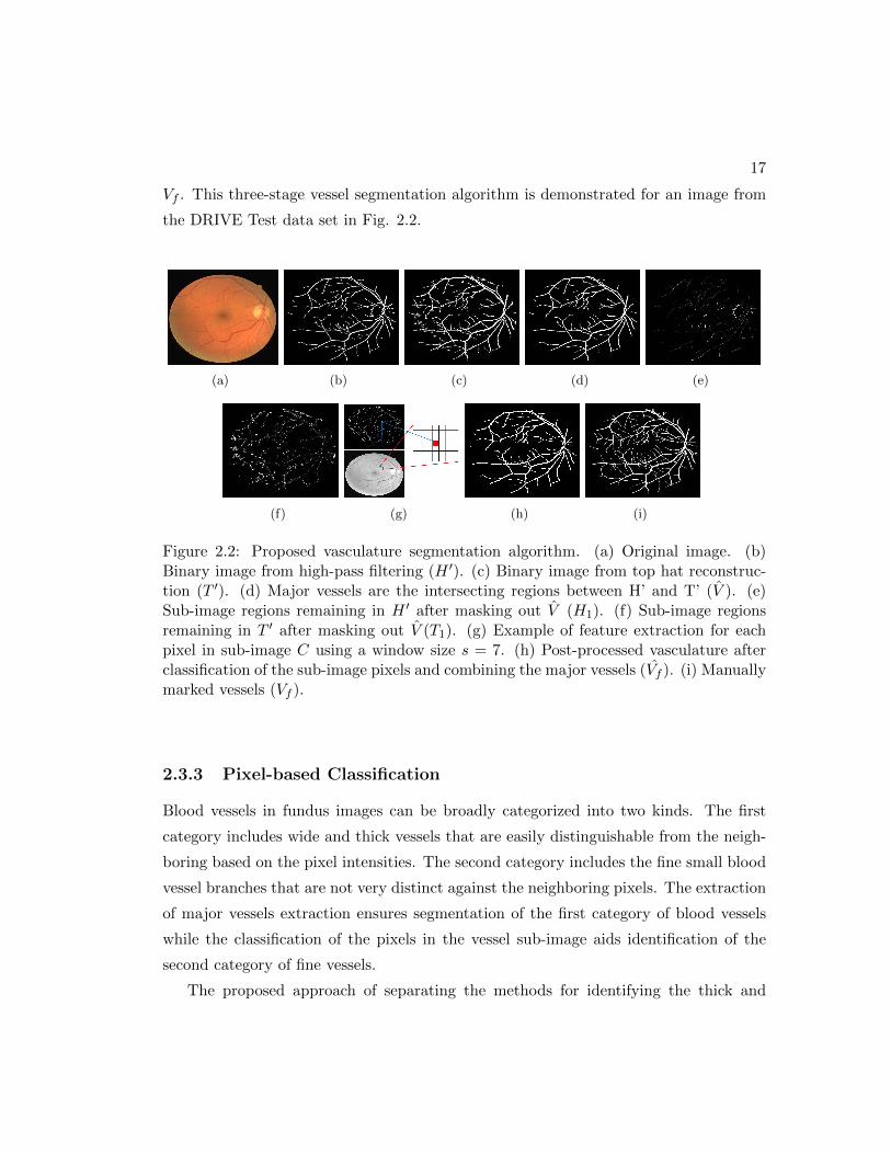
2.2 Proposed vasculature segmentation algorithm. (a) Original image. (b)

Binary image from high-pass filtering (H ′). (c) Binary image from top

hat reconstruction (T ′). (d) Major vessels are the intersecting regions be-

tween H’ and T’ (V ). (e) Sub-image regions remaining in H ′ after mask-

ing out V (H1). (f) Sub-image regions remaining in T ′ after masking out

V (T1). (g) Example of feature extraction for each pixel in sub-image C

using a window size s = 7. (h) Post-processed vasculature after classifi-

cation of the sub-image pixels and combining the major vessels (Vf ). (i)

Manually marked vessels (Vf ). . . . . . . . . . . . . . . . . . . . . . . . . 17

xii

2.3 Mean ACC and pixel classification error obtained on the validation im-

ages in the first cross-validation step. Maximum ACC and minimum

classification error occurs for a combination of 12 features and at classi-

fier threshold of 0.94. . . . . . . . . . . . . . . . . . . . . . . . . . . . . . 22

2.4 Mean ACC and pixel classification error obtained on the validation im-

ages in the second cross-validation step. Maximum ACC and minimum

classification error occurs with the top 8 voted features and classifier

threshold of 0.92. . . . . . . . . . . . . . . . . . . . . . . . . . . . . . . . 23

2.5 ROC curves for blood vessel segmentation on DRIVE test data set and

STARE data set. . . . . . . . . . . . . . . . . . . . . . . . . . . . . . . . 25

2.6 Best and worst vessel segmentation examples from the DRIVE Test,

STARE, and CHASE DB1 data sets. (a) Original image. (b) first human

observer annotation. (c) second human observer annotation. (d) Seg-

mented vessels using the proposed algorithm. In the images with worst

ACC, the segmented vessels within the region enclosed by the green cir-

cle resemble the manual annotations of the second human observer more

than the first human observer. . . . . . . . . . . . . . . . . . . . . . . . 34

2.7 Vessel segmentation on abnormal images. First row depicts vessel seg-

mentation on an image with red lesions while the second row depicts

segmentation on an image with bright lesions. (a) Image (b) Manually

marked vessels. (c) Thresholded tophat transformed image (T > 0.44).

(d) Thresholded high-pass filtered image (H > 0.36). (e) Major vessels

detected (P ). (f) Final segmented vasculature using proposed method. . 36

2.8 Comparative performance of existing methods with proposed method on

the abnormal retinal images. (a) ROC curve for the first abnormal image

with red lesions in Fig. 2.7. (b) ROC curve for the second abnormal

image with bright lesions in Fig. 2.7. . . . . . . . . . . . . . . . . . . . . 37

2.9 Peripapillary vessels segmented for the STARE set of images. (a) Second

Human Observer. (b) Marin et. al. method. (c) Soares et. al. method,

(d) Hoover et. al. method. (e) Proposed Method. . . . . . . . . . . . . . 38

xiii

3.1 The iterative vessel segmentation algorithm on an image with 45o FOV.

(a) Green plane image (I). (b) Vessel enhanced image by tophat recon-

struction (T ). (c) Major vessels extracted from T (V0). (d) Residual

image R0 with pixels from V0 removed from image T . (e) New vessel pix-

els identified by thresholding R0 (VR0). (f) Base image B0 obtained by

combining pixels in VR0 and V0 on image T . (g) V1 extracted after region-

growing. (h) Final vasculature estimate obtained after 4 iterations (Vf ).

(i) Manually marked vasculature (V ). (j) Vessel estimates extracted after

each iteration t = 3 to t = 10 by repeating steps (d) to (g) iteratively.

A stopping criterion is required to stop the iteration at t = 4 to prevent

over-segmentation. . . . . . . . . . . . . . . . . . . . . . . . . . . . . . . 62

3.2 Estimation of threshold function φ2(t) for region-growing. (a) The high-

est mean vessel segmentation accuracy (ACC l) versus the threshold func-

tion parameters [α, k]. (b) The mean iteration number (tl) correspond-

ing to highest ACC l versus threshold function parameters [α, k] on the

DRIVE Train set of images. The arrow marks the ideal choice of thresh-

old function parameters. . . . . . . . . . . . . . . . . . . . . . . . . . . 63

3.3 The stopping criterion for the iterative algorithm. If the number of iter-

ation ‘t’ is less than 3, or if the sign of the C1t , C

2t , C

3t are not all non-

negative, then iterations are continued. However, if all the first three

derivatives of C become non-negative, the iterations are stopped. . . . . 64

3.4 Theoretical example for curves corresponding to the iterative change in

blood vessels Cx and iterative error incurred Ex. The repeated root for

curves Ex, Cx occurs in the region with medium Q. As iterations proceed

beyond the repeated root, the first three derivatives of Ex and Cx become

non-negative. . . . . . . . . . . . . . . . . . . . . . . . . . . . . . . . . . 65

3.5 Change in segmented vessel estimates Ct and the iterative error incurred

Et for an image from the DRIVE Test data set along with the best fit

polynomials for Ct with degree 3 and for Et with degree 4, respectively. 65

xiv

3.6 The vessel estimate curves Ct and Et for a particular image from (a)

DRIVE Test, and (b) STARE, respectively. The stopping iterations are

(a) tf = 5, (b) tf = 4. In (a) the three consecutive derivatives for Et and

Ct become non-negative at the same iteration step. In (b), the iteration

for three consecutive non-negative derivatives corresponding to Ct and

Et are different. . . . . . . . . . . . . . . . . . . . . . . . . . . . . . . . . 66

3.7 (a) ROC curves for blood vessel segmentation on DRIVE test, STARE

and CHASE DB1 data sets. (b) Variation in mean segmentation accuracy

by varying the thresholds. Highest ACC is achieved for the DRIVE Test,

STARE and CHASE DB1 data sets with k = [1.4, 1.6, 1.6], respectively. 68

3.8 Vessel segmentation on abnormal images. First row depicts vessel seg-

mentation on an image with red lesions while the second row depicts

segmentation on an image with bright lesions. (a) Image. (b) Manually

marked vessels. (c) Segmentation by Soares et. al. (d) Segmentation by

Marin et. al. (e) Segmentation by proposed method. . . . . . . . . . . . 69

3.9 Peripapillary vessels segmented for the STARE set of images. (a) Second

Human Observer. (b) Marin et. al. method. (c) Soares et. al. method.

(d) Hoover et. al. method. (e) Proposed Method. . . . . . . . . . . . . . 70

4.1 Bright region extraction using different structuring elements for morpho-

logical transformation. Top row represents morphologically transformed

image Ir using a horizontal linear structuring element of a certain length

(Line, [pixel length]), or a circular structuring element with a certain ra-

dius (Circle, [pixel radius]). Second row represents the image containing

the bright regions obtained by thresholding the respective image Ir. For

this image from DIARETDB0 data set, a circular structuring element

with radius 17 results in the best segmented OD. . . . . . . . . . . . . . 78

xv

4.2 Steps involved in extracting the brightest OD sub-region and the OD

neighborhood. (a) Original image from DIARETDB0. (b) Morpholog-

ically reconstructed image Ir. (c) Major vessels extracted as Iv. (d)

Bright regions extracted in image Ib. (e) Intersecting bright candidate

regions (R in blue) and the vessel regions (red). (f) Solidity of regions in

R is computed. The region depicted by red arrow is discarded since that

region has ‘holes’ in it, i.e., A(Re)F (Re) < η0. The region depicted by yellow

arrow has the maximum solidity. (g) Circular discs estimate vessel-sum

within them for each region in R. The region with yellow boundary has

the maximum vessel-sum. (h) OD neighborhood detected (SROD). . . . 91

4.3 The OD boundary segmentation steps for an image from DIARETDB0

data set. (a) OD neighborhood mask (SROD). (b) Superimposed image

Ir SROD . (c) Bright regions detected in image T after thresholding

image (b). (d) The OD candidate region (ROD) is located among the

bright regions in T . (e) Bright regions in T that are close to the ROD are

retained as image P . (f) Convex hull (H) constructed around all regions

in image (e). (g) Best fit ellipse to the convex hull. (h) The segmented

OD boundary (D). . . . . . . . . . . . . . . . . . . . . . . . . . . . . . . 92

4.4 The VO pixel location steps. (a) Superimposed image SROD Iv. (b) The

centroid pixel denoted by red arrow. (c) The VO pixel located. . . . . . 93

4.5 The metrics used to evaluate the performance of automated OD segmen-

tation. . . . . . . . . . . . . . . . . . . . . . . . . . . . . . . . . . . . . . 93

4.6 Examples of automated OD segmentation performance. In both cases

S = 13 . M is estimated using 4 sample points on the actual and OD

boundaries denoted by the solid black dots. (a) has higher M than (b),

hence (b) is a better segmentation. . . . . . . . . . . . . . . . . . . . . . 93

xvi

4.7 Best and worst OD segmentation performances achieved using the pro-

posed algorithm. The first two columns demonstrate the best OD seg-

mentation cases. Third and fourth columns demonstrate the worst OD

segmentation cases. The dotted blue outline represents the manually

annotated OD (D) while the solid black circle represents the automati-

cally segmented OD (D). The cyan (*) represents the manually marked

VO (O), while the black (*) represents the automated VO detected (O).

For all the worst case performances, the automated VO lies within the

manually marked OD boundary, thereby showing that the proposed OD

segmentation algorithm has 100% ACC on all the 5 public data sets. . . 96

4.8 Examples of automated OD segmentation on images, taken from the

MESSIDOR data set, with abnormalities around the OD regions. First

column shows the original image. Second column shows the reddest and

bright region overlapping using the MaxVeSS algorithm. Third column

shows the OD neighborhood mask superimposed on the green plane image

I. Fourth column shows the bright regions (T ) in black superimposed on

the image I. The brightest OD candidate region (ROD) is indicated

by the arrow. The fifth column shows the final best-fit ellipse detected

(solid black line) and VO detected (black *) compared to the manually

segmented OD boundary (dotted blue line) and manual VO (cyan *). . 97

4.9 Histograms showing the distribution of ∆ and M in the data sets. The

red line indicates the mean values (mean (∆), mean(M)). The distribu-

tion of ∆ is shown in (a) DRIVE (b) DIARETDB1 (c) DIARETDB0 (d)

CHASE DB1 (e) MESSIDOR (500 manually annotated images). The dis-

tribution of M is shown in (f) DRIVE (g) DIARETDB1 (h) DIARETDB0

(i) CHASE DB1 (j) MESSIDOR. . . . . . . . . . . . . . . . . . . . . . . 99

4.10 Examples of images with 30o FOV that require post-processing to elimi-

nate false OD detection. (a) Original image. (b) Intersecting blood vessel

(red) and bright (blue) regions detected. (c) Automated OD boundary

and VO detected. Analysis of the thickness of the blood vessels within the

segmented OD region can be used as a post-processing step to eliminate

such false detections. . . . . . . . . . . . . . . . . . . . . . . . . . . . . 100

xvii

5.1 The three-stage algorithm for grading DR severity using fundus images.

The system flow depicts the functionalities of the three individual stages

and their interconnections. . . . . . . . . . . . . . . . . . . . . . . . . . . 106

5.2 Original blurry images are enhanced by spatial filtering. (a), (c) Fundus

image (I), (b), (d) Filtered image with enhanced red lesions marked in

red circles. . . . . . . . . . . . . . . . . . . . . . . . . . . . . . . . . . . . 108

5.3 Detection of OD, vasculature and foreground candidate regions. (a) illu-

mination corrected pre-processed image. (b) Intersecting red regions and

bright regions (blue), out of which OD is selected as the bright region

with highest solidity. (c) OD (ROD) detected. (d) vasculature (Rvasc)

detected. (e) Candidate bright lesion regions (RBL) detected. (f) Candi-

date red lesion regions (RRL) detected. . . . . . . . . . . . . . . . . . . . 122

5.4 Two-step hierarchical classification of lesions for an image from DIARETDB1.

In Stage 1 of the automated system, background regions corresponding

to vasculature and optic disc are first detected. Candidate regions for

bright (RBL) and red lesions (RRL) are then detected as the foreground.

In Stage 2, hierarchical two-step classification is performed for identifica-

tion of the type of lesions. In the first hierarchical classification step, fore-

ground regions for bright lesions are classified as true lesions (red, RTBL)

and non-lesions (blue, RNBL), and candidate regions for red lesions are

classified as true red lesions (red, RTRL) and non-lesions (blue, RNRL).

In hierarchical second-step classification, true bright lesions are classified

into hard exudates (yellow, ˆRHE), and cotton wool spots (pink, ˆRCWS),

while true red lesions are classified as microaneurysms (red, ˆRMA), and

hemorrhages (black, ˆRHA). Corresponding to the 30 features mentioned

in Table I, the average feature values for all the candidate lesion regions

in the sample image is presented in the adjoining table (i.e., f1 corre-

sponds to feature with rank 1, which is area of the region). The features

measuring distance are in terms of pixels, while the mean and variance

of intensity values are scaled in [0, 1] range. . . . . . . . . . . . . . . . . 124

xviii

5.5 DREAM system on public domain images with severe retinal degenera-

tion. (a), (d) Original image. (b), (e) OD region detected with error. (c),

(f) Vasculature detected in first stage. Both images (a), (d) are classified

as images with DR by the DREAM system. . . . . . . . . . . . . . . . . 129

6.1 Automated OD detection using the MinIMaS algorithm. (a) (c) Actual

fundus image from STARE data set. (b) (d) Segmented OD mask D

superimposed on the green plane of the actual image. . . . . . . . . . . 133

6.2 Steps for detecting laser scars and fibrosis. (a) Fundus image from

STARE data set with PDR. (b) Fundus mask ‘g’. (c) Morphologically

reconstructed bright regions in image Im. (d) Thresholded bright regions

in image T . (e) Regions satisfying the laser scar features. (f) Region

satisfying the fibrosis features. . . . . . . . . . . . . . . . . . . . . . . . . 137

6.3 Performance of the laser scar and fibrosis detection module on normal

images. (a) Normal image without PDR from the STARE data set. (b)

Morphologically reconstructed bright regions in the retinal region, i.e.,

image [Im g (1 − D)]. (c) Thresholded bright regions in image T .

There are no regions in T that satisfy the laser scar or the fibrosis features.138

6.4 Segmentation of vessel regions by watershed transform for NVD detec-

tion on an image with NVD and a normal image from the STARE data

set. (a) Image with NVD. (b) Vessel enhanced image obtained after

tophat transform (Iv). (c) Vessels within 1-disc diameter, centered at

the papilla. (d) Segmented vessel regions after watershed transform. (e)

Normal image without NVD. (f), (g), (h), correspond to images (b), (c),

(d), respectively, for the normal image. . . . . . . . . . . . . . . . . . . . 144

6.5 Example of NVE detection from an image with PDR from the STARE

data set. (a) Fundus image. (b) Vessel enhanced image (Iv). (c) Initial

vessel estimate (V0) (d) Vessel residual image after first iteration VR1 .

The region marked by the red circle satisfies all the NVE features. . . . 145

xix

6.6 Performance of NVE detection module on a normal image from the

STARE data set. (a) Normal fundus image. (b) Vessel enhanced im-

age (Iv). (c) Initial vessel estimate (V0) (d) Vessel residual image after

first iteration VR1 . (e) Vessel residual image after second iteration VR2 .

(f) Vessel residual image after third iteration VR3 . (g) Vessel residual

image after fourth iteration VR4 .(h) Vessel residual image after fifth iter-

ation VR5 . In images (d) (e) (f) (g) (h) the region in red circle satisfies the

NVE criterion regarding feature ∆1, the region in yellow circle satisfies

the NVE criterion for feature ∆3, and the region in blue dashed circle

satisfies the NVE criterion for feature ∆4. Since no region in any iter-

ation satisfies all the three criteria, hence no NVD regions are detected

for this image. . . . . . . . . . . . . . . . . . . . . . . . . . . . . . . . . 146

6.7 Distribution of the number of segmented vessel regions by watershed

transform on images with PDR and normal images from the STARE

data set. The number of segmented vessel regions for the normal images

are significantly different from that of the images with PDR. . . . . . . 147

6.8 Examples of NVD detection on images from the Local data set. (a)

Fundus image. (b) Enhanced vessels in the 1-OD diameter region. (c)

Segmented vessel regions by watershed transform. . . . . . . . . . . . . . 147

6.9 Examples of NVE detection on images from the Local data set. (a) (c)

Fundus images. (b) (d) The corresponding blood vessels extracted are

denoted in green, while the NVE regions detected are denoted in magenta.148

7.1 Sub-retinal surfaces and layers in OCT images for segmentation. The 7

sub-retinal surfaces are color coded as Surface 1 (Blue), Surface 2 (Cyan),

Surface 3(Red), Surface 4 (Yellow), Surface 5 (Pink), Surface 6 (Black),

Surface 7 (Green). The sub-retinal layers are: NFL, IPL, INL, ONL,

POS, PIS, Inner and IS/OS segments. . . . . . . . . . . . . . . . . . . . 154

xx

7.2 Steps for the proposed iterative multi-resolution segmentation algorithm

on an abnormal OCT image. (a) Denoised image by the proposed method

(Id). (b)Image I1 obtained after high-pass filtering in iteration k = 1.

Thresholding this image results in the detection of Surface 1 and the

choroidal segment(c) Negative source image 1 − Id in iteration k = 2

within the region of interest marked by G2 that extends between the

Surface 1 and the choroid segment.(d) Image obtained after high-pass

filtering and thresholding the image in (c) in iteration k = 2. The region

with maximum major axis length is extracted in image Ir2 . The top

surface of this region is Surface 5, and the bottom surface is Surface

7. (e) Image obtained in iteration k = 4 after high-pass filtering and

thresholding. The region with maximum major axis length is selected

in image Ir4 , and the bottom surface of this region is Surface 4. Two

more iterations are performed to extract all 7 surfaces. (f) Automated

segmentation achieved at the end of 6 iteration steps by the proposed

method. (g) Manually marked surfaces. (h) Automated segmentation

achieved using baseline CDWT approach for denoising followed by the

proposed segmentation algorithm. . . . . . . . . . . . . . . . . . . . . . . 170

7.3 Sub-retinal layer thickness maps for a normal OCT image stack. The first

column of images represents thickness maps generated by interpolating

the sub-retinal thickness of each layer obtained by manual annotation.

The second column of images represents the thickness maps obtained

by the proposed denoising and segmentation algorithms. The third col-

umn of images represents the thickness maps obtained by the baseline

CDWT denoising method followed by the proposed segmentation algo-

rithm. For each segmented thickness map obtained by the proposed de-

noising method and the baseline CDWT method, the mean sub-retinal

layer thickness and the correlation coefficient ‘r’ of automated thickness

distribution with respect to the manual thicknesses are provided. . . . 171

xxi

7.4 Example of automated OCT image denoising. (a) Noisy image (I), (b)

The foreground region lies within the region bordered by the red bound-

ary. All other regions are the background. (c) Denoised image by CDWT

method. (d) Denoised image by the proposed method. . . . . . . . . . . 172

7.5 Sub-retinal layer thickness maps for an abnormal OCT image stack. The

first column of images represents thickness maps generated by manual

annotation. The second column of images represents the thickness maps

obtained by the proposed method. The third column of images represents

the thickness maps obtained by the baseline CDWT method. For each

segmented thickness map obtained by the proposed denoising method and

the baseline CDWT method, the mean sub-retinal layer thickness and the

correlation coefficient ‘r’ of automated thickness distribution with respect

to the manual thicknesses are provided. . . . . . . . . . . . . . . . . . . 173

7.6 Difference between thickness maps of the INL and ONL in normal and

abnormal images with DME. . . . . . . . . . . . . . . . . . . . . . . . . 174

7.7 Irregular plateau regions observed in INL and ONL of the segmented

abnormal OCT image stack. First second and third columns indicate

thickness maps segmented manually, by the proposed method and by the

baseline CDWT methods, respectively. The combined area of irregular-

ity extracted from the INL and ONL from the manual thickness maps,

are highly correlated to the combined area of INL and ONL from the

automated segmentation methods. . . . . . . . . . . . . . . . . . . . . . 174

xxii

Chapter 1

Introduction

1.1 Introduction

Computer-aided diagnosis (CAD) has become a vital part of medical evaluations and

pathology detection in the United States [1]. Systematic use of CAD systems since 1980s

has caused a significant change in the utilization of the computer output for pathology

diagnosis, disease prognosis and treatment prioritization. Automated pathology detec-

tion and screening systems assist in interpretation of the medical signals, achieving a

baseline evaluation and automatically analyzing disease severity, which in turn helps to

prioritize patients for treatment follow-ups. Examples of popular CAD systems include

analysis of X-ray, Magnetic Resonance Imaging (MRI) and Ultrasound images.

Medical images can be considered as 2-dimensional signals from a particular part

of the human body that are accompanied by significant background noise from other

neighboring parts of the body. Thus, automated analysis of medical images involves

elegant solutions engineered from the concepts of digital signal processing and machine-

learning. Studies in [2] have shown that automated ophthalmic screening programs alone

could save the US healthcare budget nearly 400 million USD per year. Additionally,

automated prioritization of eye-care delivery could reduce time delays in treatment

by 50%, thereby significantly reducing the chances of acquired blindness [2]. With such

increasing costs of health care, research dedicated towards engineering optimal solutions

for ophthalmic image analysis will lead to faster and cheaper diagnostic systems and

cost-effective treatment delivery. An example of an existing opthalmic fundus imaging

1

2

system is shown in Fig. 1.1.

Figure 1.1: An Ophthalmic imaging system for the Retina (anterior portion of the eye).The acquired image is called a fundus image.

In this work, automated algorithms are presented for the analysis of two separate

modalities of ophthalmic images. These images capture the human retina, or the ante-

rior part of the eye that is sensitive to light and that triggers nerve impulses of vision

that are carried to the brain by the optic nerve. Retinal pathologies may be triggered

as symptoms of prolonged diseases like diabetes, hypertension, high cholesterol etc.,

causing blood vessel leakage or hemorrhaging, impacting the structure and functional-

ities of the retinal arteries or veins, accumulation of lipids on the retinal surfaces or

impacting the axiomatic plasma. If untreated or undiagnosed in a timely manner, such

retinal abnormalities can lead to acquired blindness. Examples of change in vision due

to retinal pathologies are shown in Fig. 1.2.

The first modality of retinal images analyzed in this work is retinal fundus imaging.

Fundus images typically include the optic disc (OD, head of the optic nerve), macula

(the spot which is most sensitive to vision) and blood vessels as shown in Fig. 1.3

3

Figure 1.2: Changes in vision due to retinal pathologies[Source:http://www.ucdenver.edu].

(a). Automated analysis of fundus images aids detection of abnormalities caused by

pathologies. Abnormal regions that appear due to diabetic retinopathy (DR) are shown

in Fig. 1.3 (b). Algorithms based on the principles of image denoising, spatial filtering

and segmentation can be used to separate the abnormal regions of interest followed by

machine-learning based algorithms that guide the decision making process regarding the

presence or absence of a particular retinal pathology.

Automated detection of the OD aids analysis of the changes caused by pathologies

such as Glaucoma and proliferative diabetic retinopathy (PDR). Automated segmenta-

tion of blood vessels helps analysis of the blood vessel width, vessel density, tortuosity

etc. for detection of disease such as PDR, Retinopathy of Prematurity (RoP), retinal

vein occlusions (RVO) and age-related macular degeneration (AMD). Also, detection of

4

(a) (b)

Figure 1.3: Example of fundus images. (a) Anatomy of a fundus image. (b) Abnormal-ities in fundus image due to DR.

bright and red abnormalities that occur as manifestation of non-proliferative diabetic

retinopathy (NPDR) using automated algorithms can help screening and prioritization

of patients based on disease severity.

The second modality of images under analysis is acquired using Optical Coherence

Tomography (OCT). An example of OCT images is shown in Fig. 1.4. This imaging

modality captures the micrometer-resolution of the third dimension, or the depth of

retinal tissue. OCT is an interferometric technique that measures the depth of sub-

retinal layers in the form of lateral scans. These lateral scans when combined can

represent the 3-dimensional view of the retina that can be then used to locate and treat

macular pathologies. Automated segmentation and analysis of OCT images can aid

clinical studies regarding the progression of diseases over time, the impact of treatment

and pathology localization for laser surgeries.

5

Figure 1.4: Example of the OCT imaging modality. Several lateral scans are combinedto obtain a 3-D retinal microstructure.

1.2 Summary of Contributions

The automated segmentation and pathology detection algorithms presented in this the-

sis can be beneficial for assisting primary eye-care providers in obtaining a quick au-

tomated screening result or semi-automated screening capability for diseases such as

diabetic retinopathy (DR). Also, telemedicine, with distributed, remote retinal fundus

imaging in local primary care offices and centralized grading by eye care specialists may

increase access to screening and thus necessary treatment [3]. Automated retinal screen-

ing systems such as the ones proposed in this thesis will help augment a telemedicine

approach using a web-based interface, where retinal images can be uploaded, that results

in end reports that can be then analyzed by specialists to provide quicker evaluations.

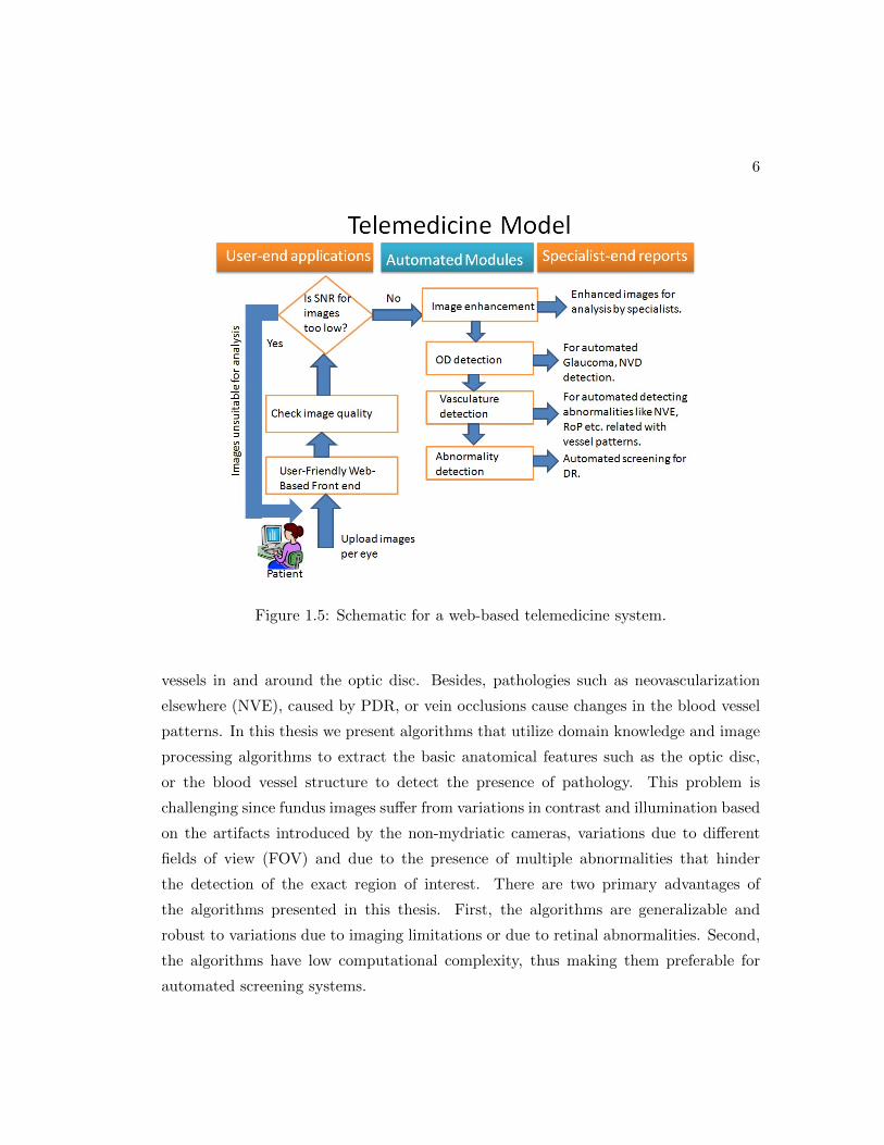
An example of such a web-based telemedicine system is shown in Fig. 1.5.

Our main contributions can be classified under three main categories: automated

segmentation of various anatomical regions of fundus images, automated screening sys-

tems for detecting severity and presence of pathologies such as NPDR and PDR using

fundus images, and automated segmentation of the sub-retinal micro-structure to aid

clinical analysis of OCT images from patients with diabetic macular edema (DME). The

contributions made in each of these categories are summarized below.

1.2.1 Segmentation of Retinal Anatomical Regions in Fundus Images

Certain retinal pathologies cause variations in the anatomical regions in fundus images.

For instance, glaucoma causes variation in the cup-to-disc ratio of the optic disc, or

neovascularization at the disc (NVD) caused by PDR, causes a dense mesh of new blood

6

Figure 1.5: Schematic for a web-based telemedicine system.

vessels in and around the optic disc. Besides, pathologies such as neovascularization

elsewhere (NVE), caused by PDR, or vein occlusions cause changes in the blood vessel

patterns. In this thesis we present algorithms that utilize domain knowledge and image

processing algorithms to extract the basic anatomical features such as the optic disc,

or the blood vessel structure to detect the presence of pathology. This problem is

challenging since fundus images suffer from variations in contrast and illumination based

on the artifacts introduced by the non-mydriatic cameras, variations due to different

fields of view (FOV) and due to the presence of multiple abnormalities that hinder

the detection of the exact region of interest. There are two primary advantages of

the algorithms presented in this thesis. First, the algorithms are generalizable and

robust to variations due to imaging limitations or due to retinal abnormalities. Second,

the algorithms have low computational complexity, thus making them preferable for

automated screening systems.

7

1.2.2 DR Screening Systems using Funds Images

Guidelines from the American Diabetes Association (ADA) specify that all patients with

diabetes must be screened annually for DR. However, 90% of the images thus acquired

has no signs of DR. Thus, automated screening systems for DR can be used to screen the

patients with DR and thereby help to prioritize and enhance the resourcefulness of eye-

care delivery. In this thesis, we introduce the DREAM (Diabetic Retinopathy Analysis

using Machine Learning [3]) system that is capable of screening patients with mild,

moderate to severe NPDR from the patients with no DR. Another screening system

that detects the presence of PDR based on the presence of post-operative laser scar

marks, fibrosed tissue, NVD or NVE is also presented.

1.2.3 Automated Segmentation of OCT images

OCT images typically suffer from low signal to noise ratio (SNR) owing to the micron-

level resolution of the images. Additionally, pathologies such as DME causes variations

in the retinal micro-structure poses challenges for automated segmentation algorithms

that are robust to both normal and pathological OCT images. In this thesis, we present

automated denoising and segmentation algorithms that utilize adaptive thresholds for

enhancing the image SNR and segmenting the sub-retinal layers in normal and abnormal

OCT images with DME. These algorithms can be beneficial for conducting clinical

studies that monitor the progression of pathology over time.

1.3 Outline of this Thesis

The thesis is outlined as follows. An automated blood vessel segmentation algorithm

that uses pixel-based classification for vessel detection is presented in Chapter 2. The

pixel-based features that are capable of discriminating finer vessel pixels from the back-

ground pixels are described.

Chapter 3 introduces an iterative algorithm that iteratively detects and adds fine

blood vessels to an existing vessel estimate using fundus images. This iterative algorithm

is capable of detecting fine blood vessels with high precision in pathological images.

Chapter 4 presents a rule-based algorithm for detecting the OD in normal and

8

pathological fundus images. This algorithm detects the exact OD boundary and the

point of vessel origin.

Chapter 5 presents the DREAM system for screening images with NPDR from the

images without any retinopathy. This three-stage system separates the image back-

ground from the foreground, identifies region-based features that discriminate bright

lesions and red lesions that are caused by NPDR, and grades the severity of NPDR.

Chapter 6 presents a screening system for detection of PDR. This system utilizes

the iterative vessel segmentation algorithm from Chapter 3 to detect the fine vessel

structures followed by rule-based decision regarding the presence of NVD and NVE.

Also the presence of laser scars and fibrosis are detected in fundus images.

Chapter 7 presents an automated denoising and segmentation system for OCT image

stacks. OCT stacks from healthy eyes and pathological eyes (with DME) are segmented

to extract seven sub-retinal surfaces and six sub-retinal layers. Thickness maps con-

structed from the segmented sub-retinal layers from an OCT stack of images are also

analyzed.

Finally, Chapter 8 presents conclusions regarding all the automated algorithms pre-

sented in this thesis and provides directions for future work.

Chapter 2

Automated Vessel Segmentation:

A Classification Approach

2.1 Introduction

Analysis of the retinal blood vessels (vasculature) from fundus images has been widely

used by the medical community for diagnosing complications due to hypertension, ar-

teriosclerosis, cardiovascular disease, glaucoma, stroke and diabetic retinopathy (DR)

[4]. According to the American Diabetes Association, DR and glaucoma are the leading

causes of acquired blindness among adults aged 20-74 years with estimates of 4.2 million

Americans having DR and 2.3 million having glaucoma in 2011 [5]. Automated blood

vessel segmentation systems can be useful in determining variations in the blood ves-

sels based on the vessel branching patterns, vessel width, tortuosity and vessel density

as the pathology progresses in patients [6]. Such analyses will guide research towards

analyzing patients for hypertension [7], variability in retinal vessel diameters due to a

history of cold hands and feet [8], and flicker responses [9].

Existing automated detection systems for non-proliferative DR detection, such as

[10] [3], require masking of the vasculature to ensure that the blood vessels are not

mistaken for red lesions that are caused by DR. Also, automated detection of prolif-

erative DR requires analysis of the density, vessel width and tortuosity of the blood

vessels. A fast and accurate segmentation algorithm for detecting the blood vessels is

necessary for such automated detection and screening systems for retinal abnormalities

9

10

such as DR. Some existing unsupervised vessel segmentation methods have achieved

up to 92% segmentation accuracy on normal retinal images by line-detector and tem-

plate matching methods [11] that are computationally very fast. However, increasing

the segmentation accuracy above 92% for abnormal retinal images with bright lesions

(exudates and cotton wool spots), or red lesions (hemorrhages and microaneurysms),

or variations in retinal illumination and contrast, while maintaining low computational

complexity is a challenge. In this chapter we separate the vessel segmentation problem

into two parts, such that in the first part, the thick and predominant vessel pixels are

extracted as major vessels and in the second part, the fine vessel pixels are classified

using neighborhood-based and gradient-based features.

This chapter makes two major contributions. First, the number of pixels under

classification is significantly reduced by eliminating the major vessels that are detected

as the regions common to thresholded versions of high-pass filtered image and morpho-

logically reconstructed negative fundus image. This operation is key to more than 90%

reduction in segmentation time complexity compared to the existing methods where all

the vessel pixels are classified in [12], [13]. Additionally, the proposed method is more

robust to vessel segmentation in abnormal retinal images with bright or red lesions than

thresholded high-pass filtered and tophat reconstructed images. The second major con-

tribution is the identification of an optimal 8-feature set for classification of the fine

blood vessel pixels using the information regarding the pixel neighborhood and first

and second-order image gradients. These features reduce the dependence of vessel pixel

classification on the training data and enhance the robustness of the proposed vessel

segmentation for test images with 45o, 35o and 30o fields of view (FOV), and for images

with different types of retinal abnormalities.

The organization of this chapter is as follows. In Section 2.2, the existing automated

vessel segmentation algorithms in the literature are reviewed. The proposed method

and materials are described in Section 2.3. In section 2.4, the experimental setup for

analyzing the performance of vessel segmentation and results are presented. Finally, in

Section 2.5, discussion and conclusions are presented.

11

2.2 Prior Work

The problem of automated segmentation of retinal blood vessels has received significant

attention over the past decade [14]. All prior works for vasculature segmentation can

be broadly categorized as unsupervised and supervised approaches.

In the unsupervised methods category, algorithms that apply matched filtering, ves-

sel tracking, morphological transformations and model-based algorithms are predomi-

nant. In the matched filtering-based method in [15], a 2-D linear structuring element is

used to extract a Gaussian intensity profile of the retinal blood vessels, using Gaussians

and their derivatives, for vessel enhancement. The structuring element is rotated 8-12

times to fit the vessels in different configurations to extract the boundary of the vessels.

This method has high time complexity since a stopping criterion is evaluated for each

end pixel. In another vessel tracking method [16], Gabor filters are designed to detect

and extract the blood vessels. This method suffers from over-detection of blood vessel

pixels due to the introduction of a large number of false edges. A morphology-based

method in [17] combines morphological transformations with curvature information and

matched-filtering for center-line detection. This method has high time complexity due to

the vessel center-line detection followed by vessel filling operation, and it is sensitive to

false edges introduced by bright region edges such as optic disc and exudates. Another

morphology based method in [18] uses multiple structuring elements to extract vessel

ridges followed by connected component analysis. In another model-based method [19],

blood vessel structures are extracted by convolving with a Laplacian kernel followed by

thresholding and connecting broken line components. An improvement of this method-

ology was presented in [20], where the blood vessels are extracted by the Laplacian

operator and noisy objects are pruned according to center lines. This method focuses

on vessel extraction from images with bright abnormalities, but it does not perform very

effectively on retinal images with red lesions (such as hemorrhages or microaneurysms).

The method in [21] presents perceptive transformation approaches to segment vessels

in retinal images with bright and red lesions.

A model-based method in [22] applies locally adaptive thresholding and incorpo-

rates vessel information into the verification process. Although this method is more

12

generalizable than matched-filter based methods, it has a lower overall accuracy. An-

other model-based vessel segmentation approach proposed in [23] uses active contour

models, but suffers from computational complexity as well. Additionally, multi-scale

vessel segmentation methods proposed in [24] and [25] use neighborhood analysis and

gradient-based information for determining the vessel pixels. All such unsupervised

methods are either computationally intensive or sensitive to retinal abnormalities.

The supervised vessel segmentation algorithms classify pixels as vessel and non-

vessel. In [26], the k-Nearest Neighbor (kNN) classifier uses a 31-feature set extracted

using Gaussians and their derivatives. The approach in [27] improved this method

by applying ridge-based vessel detection. Here each pixel is assigned to its nearest

ridge element, thus partitioning the image. For each pixel, a 27 feature set is then

computed and is used by a kNN classifier. Both these methods are slowed down by

the large size of the feature sets. Also, these methods are training data dependent and

sensitive to false edges. Another method presented in [28] uses Gaussian Mixture Model

(GMM) classifier and a 6-feature set extracted using Gabor-wavelets. This method is

also training data dependent, and it requires hours for training GMM models with a

mixture of 20 Gaussians. The method in [29] uses line operators and a support vector

machine (SVM) classifier with a 3-feature set per pixel. This method is very sensitive

to the training data and is computationally intensive due to the SVM classifiers. The

method in [12] applies boosting and bagging strategies with 200 decision trees for vessel

classification using a 9-feature set extracted by Gabor filters. This method suffers from

high computational complexity as well due to the boosting strategy. The only other

supervised method that is independent of the training data set is proposed in [13]

that applies neural network classifiers using a 7-feature set extracted by neighborhood

parameters and a moment invariants-based method. The proposed vessel segmentation

method is motivated by the method in [13] to design a segmentation algorithm that

has low dependence on training data and is computationally fast. So far, computational

complexity of vessel segmentation algorithms has been addressed only in [11] and [21]. In

this chapter we reduce the number of pixels under classification, and identify an optimal

feature set to enhance the consistency in the accuracy of blood vessel segmentation, while

maintaining a low computational complexity.

13

2.3 Method and Materials

For every color fundus photograph, the proposed vessel segmentation algorithm is per-

formed in three stages. In the first stage, two thresholded binary images are obtained:

one by high-pass filtering and another by tophat reconstruction of the red regions in

the green plane image. The regions common to the two binary images are extracted

as the major vessels and the remaining pixels in both binary images are combined to

create a vessel sub-image. In the second stage, the pixels in the vessel sub-image are

subjected to a 2-class classification. In the third post-processing stage, all the pixels

in the sub-image that are classified as vessels by the classifier are combined with the

major vessels to obtain the segmented vasculature. Depending on the resolution of the

fundus images, in the post-processing stage, the segmented vessels are further enhanced

to ensure higher vessel segmentation accuracy. Here, the proposed vessel segmentation

algorithm is evaluated using three publicly available data sets.

2.3.1 Data

The vessel segmentation algorithm is trained and tested with the following data sets

that have been manually annotated for the blood vessel regions.

• STARE [15] data set contains 20 images with 35o FOV that are manually anno-

tated by two independent human observers. Here, 10 images represent patients

with retinal abnormalities (STARE Abnormal). The other 10 images represent

normal retina (STARE Normal).

• DRIVE [27] data set contains 40 images with 45o FOV. This data set is separated

by its authors into a training set (DRIVE Train) and a test set (DRIVE Test)

with 20 images in each set. The DRIVE Train set of images are annotated by one

human observer while the DRIVE Test data set is annotated by two independent

human observers.

• CHASE DB1 [30] data set contains 28 images with 30o FOV corresponding to two

images per patient (one image per eye) for 14 children. Each image is annotated

by two independent human observers [12].

14

2.3.2 Problem Formulation

The first pre-processing stage requires the green plane of the fundus image scaled in [0,

1] (I), and a fundus mask (g). In the green plane image, the red regions corresponding

to the blood vessel segments appear as dark pixels with intensities close to 0. In such

cases, the fundus mask removes the dark background region from the photographs and

helps to focus attention to the retinal region only. The fundus mask is superimposed on

image I followed by contrast adjustment and vessel enhancement, resulting in a vessel

enhanced image Ie. The vessel enhancement operation involves squaring each pixel

intensity value and re-normalizing the image in [0, 1] range thereafter. This is a vital

operation since the dark pixels corresponding to the vessel regions (with pixel values

closer to 0), when squared, become darker, while the non-vessel bright regions become

brighter, hence resulting in the enhancement of the blood vessel regions.

To extract the dark blood vessel regions from Ie, two different pre-processing strate-

gies are implemented. First, a smoothened low-pass filtered version of Ie (LPF (Ie)) is

subtracted from Ie to obtain a high-pass filtered image. Here, the low-pass filter is a

median filter with window size [20x20] as used in [10] [31]. This high-pass filtered im-

age is thresholded to extract pixels less than 0, and the absolute pixel strengths of the

thresholded image are contrast adjusted to extract the vessel regions. This is referred to

as the pre-processed image H (2.1). For the second pre-processed image, the red regions

corresponding to the dark pixels are extracted from the negative of image Ie, thus result-

ing in image R. Next, 12 linear structuring elements each of length 15 pixels and 1 pixel

width and angles incremented by 15o from 0 through 180o are used to generate tophat

reconstructions of R [17] [12]. The length of 15 pixels for the linear structuring element

is chosen to approximately fit the diameter of the biggest vessels in the images [12].

For each pixel location, the reconstructed pixel with the highest intensity is selected,

thereby resulting in image T (2.2). An example of the two pre-processed images H and

T is shown in Fig. 2.1. These two pre-processed images H, and T can be thresholded to

obtain baseline unsupervised models to analyze the importance of the proposed method

in the following sections. Both the pre-processed images H and T are thresholded for

pixel values greater than ‘p’ to obtain binary images H ′ and T ′ (2.3-2.4). For images

from DRIVE and STARE and CHASE DB1 data sets, ‘p = 0.2’, which ensures the red

regions to be highlighted in the vessel enhanced binary images. Next, the intersecting

15

regions between the pre-processed binary images H ′ and T ′ are retained as the major

portions of the blood vessels, or the major vessels (V ) (2.5). Once the major vessels are

removed from the two binary images, the resulting images are called vessel sub-images

H1 corresponding to binary image H ′ (2.6) and sub-image T1 corresponding to binary

image T ′ (2.7), respectively. These steps are summarized in equations (2.1)-(2.7).

In the second stage, the pixels in sub-images H1 and T1 are combined to form a

vessel sub-image C (2.8), and the pixels in C are classified using a GMM classifier that

classifies each pixel as vessel (class 1) or non-vessel (class 0). Thus, for all pixels in C,

a GMM classifier is trained once using the images from the DRIVE Train set of images

and tested on the DRIVE Test image set, STARE image set, and CHASE DB1 image

set, independently, to identify the vessel pixels in each test image. The optimal feature

set selection for vessel pixel classification is described in the following subsection. The

pixels in sub-image C that are classified as vessel result in image V ′ (2.9).

∀(x, y), H(x, y) = abs(Ie(x, y)− LPF (Ie(x, y)) < 0) (2.1)

R = (1− Ie) g, T = tophat(R) (2.2)

∀(x, y), H ′(x, y) =

1 : H(x, y) > p

0 : Otherwise.(2.3)

T ′(x, y) =

1 : T (x, y) > p

0 : Otherwise.(2.4)

V (x, y) =

1 : H(x, y) = T (x, y) = 1

0 : Otherwise.(2.5)

⇒ V = H ′ ∩ T ′.

H1(x, y) =

1 : H ′(x, y) = 1 & V (x, y) = 0

0 : Otherwise.(2.6)

T1(x, y) =

1 : T ′(x, y) = 1 & V (x, y) = 0

0 : Otherwise.(2.7)

16

(a) (b) (c) (d)

Figure 2.1: Each fundus image is subjected to contrast adjustment and pixel enhance-ment followed by high-pass filtering and tophat reconstruction. (a) Contrast adjustedvessel enhanced image (Ie). (b) High-pass filtered image (H). (c) Red regions enhancedimage (R). (d) Tophat reconstructed version of R (T ).

C(x, y) =

1 : H1(x, y) = 1 or T1(x, y) = 1

0 : Otherwise.(2.8)

⇒ C = H1 ∪ T1.

V ′(x, y)← GMMclassify(C(x, y)). (2.9)

Vf = V ∪ V ′. (2.10)

In the third post-processing stage, sub-image V ′ representing all the pixels in C that

are classified as vessel, are combined with the major vessels V to obtain the segmented

vasculature Vf (2.10). Finally, the complete segmented blood vessel Vf is post-processed

such that the regions in the segmented vasculature with area greater that ‘a’ are retained

while smaller regions are discarded. The values of ‘a’ were empirically determined as [20,

40, 50], for the images from DRIVE, STARE and CHASE DB1 data sets, respectively.

The images from the CHASE DB1 data set are different from the DRIVE and

STARE set of images since all these images are centered at the papilla and they have

thicker blood vessels. Hence, to post-process images from CHASE DB1 data set, the

segmented vasculature Vf is superimposed on the tophat reconstructed image T , and

the resulting image (Vf T ) is region grown at pixel threshold value 240 followed by

vessel filling [13]. The performance of vasculature segmentation on each image is then

analyzed with reference to manually marked blood vessels by human observers in image

17

Vf . This three-stage vessel segmentation algorithm is demonstrated for an image from

the DRIVE Test data set in Fig. 2.2.

(a) (b) (c) (d) (e)

(f) (g) (h) (i)

Figure 2.2: Proposed vasculature segmentation algorithm. (a) Original image. (b)Binary image from high-pass filtering (H ′). (c) Binary image from top hat reconstruc-tion (T ′). (d) Major vessels are the intersecting regions between H’ and T’ (V ). (e)Sub-image regions remaining in H ′ after masking out V (H1). (f) Sub-image regionsremaining in T ′ after masking out V (T1). (g) Example of feature extraction for eachpixel in sub-image C using a window size s = 7. (h) Post-processed vasculature afterclassification of the sub-image pixels and combining the major vessels (Vf ). (i) Manuallymarked vessels (Vf ).

2.3.3 Pixel-based Classification

Blood vessels in fundus images can be broadly categorized into two kinds. The first

category includes wide and thick vessels that are easily distinguishable from the neigh-

boring based on the pixel intensities. The second category includes the fine small blood

vessel branches that are not very distinct against the neighboring pixels. The extraction

of major vessels extraction ensures segmentation of the first category of blood vessels

while the classification of the pixels in the vessel sub-image aids identification of the

second category of fine vessels.

The proposed approach of separating the methods for identifying the thick and

18

fine blood vessel regions enhances the robustness of vessel segmentation on normal and

abnormal retinal images in two ways. First, the major vessel regions comprising of 50-

70% of the total blood vessel pixels are segmented in the first stage, thereby significantly

reducing the number of sub-image vessel pixels for classification. This reduction in the

number of vessel pixels under classification reduces the computational complexity and

vessel segmentation error when compared to methods that classify all major and fine

vessel pixels alike [13] [12] [29]. Second, the optimal feature set identified for sub-image

vessel pixel classification are discriminative for the fine vessel pixel segmentation. These

features aid elimination of sub-image vessel pixels from large red lesions and false bright

lesion edges in retinal images with pathology.

The most important aspect of sub-image vessel pixel classification is identification

of features that classify the fine vessel pixels from false edge pixels. Hence, we analyze

the performance of pixel-based features that distinguish a vessel pixel from its imme-

diate neighborhood, and select an optimal feature set that is suitable for fine vessel

segmentation in fundus images regardless of their FOV, illumination variability and ab-

normality due to pathology. These features under analysis and the method for selecting

the optimal feature set are described below.

Feature Description

For each pixel ‘(x,y)’ in vessel sub-image C, 57 features are analyzed to detect a dis-

criminative optimal feature set for classifying the vessel pixels. These features utilize

the information regarding the pixel neighborhood and pixel gradient to identify a fine

vessel pixel from false edge pixels. The neighborhood-based features under analysis are

motivated from the supervised segmentation method in [13] where major and fine vessel

pixels are classified alike. The gradient-based features have been analyzed in [25] [24]

for multi-level vessel pixel identification. In this chapter, the goal is to identify discrim-

inating features for fine vessel classification specifically, and hence, we analyze a range

of neighborhood-based features to select the optimal feature set using images from the

DRIVE Train data set.

For extracting the neighborhood-based features for each vessel sub-image pixel ‘(x,y)’,

5 features are defined by placing the desired pixel ‘(x,y)’ as the central pixel in a square

window of side-length ‘s’ pixels on image Ie. This 2-D window is represented as W s(x,y),

19

where the window side length ‘s’ can be varied. We limit the size s to less than 15 pixels

since the width of the widest vessel is about 15 pixels in the DRIVE Train data set. The

first 4 features (f1 to f4) are determined by mean, standard deviation, maximum pixel

intensity and minimum pixel intensity among all pixels extracted in the windowed-image

IW s

(x,y)e , and are described in (2.11)-(2.13). These features are motivated from the prior

work [13], where s = 9. The fifth new feature (f5) introduced in this chapter is a rel-

ative neighborhood discriminator feature. False edges that are introduced by the edges

of bright regions such as exudates and optic disc are discriminated by this function.

f1(s) = mean(IW s

(x,y)e ), f2(s) = std. dev(I

W s(x,y)

e ), (2.11)

f3(s) = max(IW s

(x,y)e ), f4(s) = min(I

W s(x,y)

e ). (2.12)

ν(s) = #pixels in IW s

(x,y)e ,

ν1(s) = [#pixels in IW s

(x,y)e > Ie(x, y)], f5(s) =

ν1(s)

ν(s).

(2.13)

Two other neighborhood-based features, from the prior work [13], that extract

moment-invariants based information are defined as f6 and f7. For extracting these

two features, a square windowed-image with side-length s and centered at pixel ‘(x,y)’

is extracted from the tophat reconstructed image T . In this windowed-image (TW s

(x,y)),

the ‘(p+q)’th order moments for second-order moments are defined in (2.14)-(2.17).

Here p+ q = 2. Corresponding to each pixel, the second-order moments invariant-based

features f6 and f7 as the window side length varies are given in (2.18)-(2.19).

20

∀(x, y), (p, q) = (0, 2), (1, 1), (2, 0) , (2.14)

mpq(s) =∑u

∑v

upvqTW s

(x,y)(u, v). (2.15)

µp,q(s) =∑u

∑v

(u− u)p(v − v)qTW s

(x,y)(u, v). (2.16)

ηpq(s) =µpq(s)

µ00(s)γ, γ =

p+ q

2+ 1 = 2. (2.17)

θ1(s) = η20(s) + η02(s), f6(s) = |log(θ1(s)))|. (2.18)

θ2(s) = (η20(s) + η02(s))2 + 4η11(s)2,

f7(s) = |log(θ2(s)))|. (2.19)

The 7 features f1(s) to f7(s) are evaluated for each vessel sub-image pixel by vary-

ing window side-lengths s = [3, 5, 7, 9, 11, 13, 15]. Also, the pixel intensity Ie(x, y) is

another feature. Along with the 50 neighborhood-based features mentioned above, 7

additional gradient based features are also analyzed for vessel pixel classification. For

these gradient-based features, the first and second-order gradient images of Ie are ex-

tracted. The first-order gradient images in the horizontal and vertical direction are

extracted as gh and gv, respectively. Next, the second-order gradient images in the

horizontal, vertical, and both directions are extracted as ghh, gvv, ghv, respectively. The

pixel intensity in the ‘(x,y)’ location of these first and second-order gradient images

are 5 gradient-based features. The final two gradient-based features are the Eigen val-

ues obtained by the Eigen decomposition of matrix G that is formed using the pixel

intensities from the second-order gradient images as shown in (2.20).

G =

[ghh(x, y) ghv(x, y)

gvh(x, y) gvv(x, y)

]. (2.20)

Feature Selection

To select the most discriminating features from the 57 pixel-based features described

above, we performed feature ranking and leave-one-out double cross-validation [32] on

the 20 images from the DRIVE Train data set using GMM classifiers with 2-Gaussians

(Gaussian with class label 0 corresponds to non-vessel pixels, Gaussian with class label

21

1 correspond to vessel pixels). In the first cross-validation step, one image is selected

as the validation image and the pixels from its vessel sub-image are used to generate

the validation data set. Pixels from the remaining 19 images are used to generate the

training data set, hence the name leave-one-out. Corresponding to the 20 images from

DRIVE Train data set, 20 such training/validation data sets are thus generated. Each

training data set is then subjected to feature ranking using the minimal-redundancy-

maximal-relevance (mRMR) criterion [33].

The mRMR criterion is based on mutual information from the individual features,

such that, the features are ranked based on the top combination of features that have

maximum relevance with the sample class labels and minimum redundancy. The mRMR

criterion is chosen for feature ranking over other ranking strategies such as F-score or

AdaBoost [32] since the neighborhood-based pixel features are mutually dependent, and

the mRMR criterion aims at maximizing the information from these dependent features

instead of ranking features independently.

Once the features from the training data set are ranked, GMM classifiers are trained

using the top ‘F’ ranked features, and the classifier is tested on the validation data set.

As F is varied from 1 to 57, and the threshold for GMM classifier is varied from 0 to

1 in increments of 0.01, the mean vessel segmentation accuracy (ACC) and the mean

pixel classification error across each of the 20 validation images is shown in Fig. 2.3. In

Fig. 2.3, we observe that the highest mean ACC = 0.9541 and least mean classification

error= 0.0961 occurs at a threshold of 0.94 with a combination of top 12 features.

Since the feature ranking is done separately for each of the 20 training/validation

data sets, hence the top 12 features appearing in each of the 20 sets may be different.

To identify the optimal feature set that are common to all the training/validation data

sets, feature voting is performed. We observe that by selecting the top F features for

each of the 20 training/validation data sets, F1 unique features are identified across the

20 training data sets. By varying F = [2, 3, 4, 5, 6, 7, 8, 9, 10], we observe the variation in

the number of uniquely identified features is F1 = [9, 10, 11, 16, 20, 23, 27, 31, 33]. Here,

we observe that by selecting the top 5 features for each training data set, a total of

16 features are uniquely identified. The number of occurrences for each of these 16

features among the 20 training/validation data sets is considered as the feature vote.

These 16 features are ranked in decreasing order of their feature vote. In the second

22

Figure 2.3: Mean ACC and pixel classification error obtained on the validation images inthe first cross-validation step. Maximum ACC and minimum classification error occursfor a combination of 12 features and at classifier threshold of 0.94.

cross-validation step, these top 16 voted features are re-analyzed by leave-one-out cross-

validation.

For the second cross-validation step, 20 training/validation data sets are re-generated

using the top 16 voted features and the mean ACC and classification error on the

validation images are shown in Fig. 2.4. In Fig. 2.4 we observe that, the highest mean

ACC = 0.9540 and lowest mean pixel classification error= 0.1067 occurs at a threshold

of 0.92 with a combination of top 8 features. These top 8 voted features and their

respective votes are given in Table 2.1. At the end of the cross-validation, the 8 top

features identified include four neighborhood-based features and four gradient-based

features. These 8 features will henceforth be used for classification of vessel pixels from

the vessel sub-image derived from test data sets.

2.4 Experimental Evaluation and Results

The performance of the proposed vessel segmentation algorithm is evaluated using the

segmented vasculature and the manually marked vessels by the human observers. While

manual vessel segmentation can take more than 2 hours [27], automated vessel segmen-

tation algorithms aim to reduce the manual labor while maintaining acceptable accuracy

23

Figure 2.4: Mean ACC and pixel classification error obtained on the validation imagesin the second cross-validation step. Maximum ACC and minimum classification erroroccurs with the top 8 voted features and classifier threshold of 0.92.

of vessel segmentation. All prior works have used the manual segmentations of the first

human observer for segmentation performance analysis. The vessel segmentation per-

formance of the second human observer with respect to the first human observer within

the retinal region is used to standardize the segmentation process.

The performance metrics for assessing the efficiency of the vessel segmentation is

computed in terms of the number of vessel pixels that are correctly classified as vessels

(true positives, TP), or non-vessels (true negatives, TN), pixels falsely classified as ves-

sels (false positives, FP) and pixels falsely classified as non-vessels (false negatives, FN).

Thus, the performance metrics are: pixel-based sensitivity (SEN), specificity (SPEC),

ACC of vessel segmentation along with the Area Under the Receiver Operating Charac-

teristic curve (AUC) obtained by varying the threshold in a GMM classifier in steps of

0.02 in range [0,1] [13]. The vessel segmentation time required per image in seconds for

implementing the proposed segmentation system in MATLAB on a Laptop with Intel

Core i3 processor, 2.6GHz and 2GB RAM is also recorded. The performance metrics of

the proposed system are also compared to existing works in the following subsections.

For complete assessment of the proposed supervised vessel segmentation algorithm,

we performed the following four sets of experimental evaluations. In the first experi-

ment, the performance metrics of the overall vessel segmentation algorithm is analyzed

24

Table 2.1: Optimal feature set identified by feature voting and leave-one-out doublecross validation.

Rank Vote Feature Meaning

1 20 f3(3) Maximum pixel value in a square window of side length 3.

2 17 ghv Second-order gradient in horizontal and vertical directions.

3 13 gv First-order gradient in the vertical direction.

4 12 f1(5) Mean pixel value within a square window of side length 5.

5 7 gh First-order gradient in the horizontal direction.

6 6 f2(5) Standard deviation of pixels in a square window of length 5.

7 6 f5(5) Relative neighborhood discriminator in a square windowof side length 5.

8 6 ghh Second-order gradient in the horizontal direction.

for all the three data sets. In the second experiment, the segmentation performance of

the proposed method on abnormal retinal images is analyzed. In the third experiment,

the dependence of the training data set on the vessel segmentation algorithm is ana-

lyzed by inter-changing the training and test data sets. In the fourth experiment, the

performance of blood vessel segmentation in the peripapillary region is analyzed to as-

sess the importance of the proposed vessel segmentation system for retinal abnormality

detection.

2.4.1 Vessel Segmentation Performance

For the proposed vasculature segmentation algorithm, the GMM classifier is trained

once with 8 pixel-based features using the vessel sub-images from the DRIVE Train set

of images and then subsequent testing of vessel segmentation performance is performed

on images from the DRIVE Test, STARE and CHASE DB1 data sets, separately. In

the proposed approach, the GMM classifier aids segmentation of fine blood vessels only

and hence it does not need to be retrained on incoming test data set samples. This re-

duces the dependency of the proposed segmentation algorithm on the training data set

when compared to existing supervised approaches where test images are sub-sampled

to re-train classifiers [12] [29]. Since GMM classifiers are probabilistic in nature, the

25

vessel segmentation ACC varies with the threshold. The Receiver Operating Charac-

teristic (ROC) curves in Fig. 2.5 demonstrate the variation in SEN and SPEC of vessel

segmentation as classifier threshold varies. We observe that the DRIVE Train data set

achieved highest segmentation ACC at a threshold on 0.92 but the test data sets do not

achieve best segmentation SEN/SPEC at threshold probability 0.92. For the DRIVE

Test, STARE and CHASE DB1 data sets, the optimal threshold probability values are

[0.92, 0.86, 0.82], respectively.

Figure 2.5: ROC curves for blood vessel segmentation on DRIVE test data set andSTARE data set.

The performance of blood vessel segmentation for the three test data sets is given in

Table 2.2. To analyze the incremental importance of the proposed supervised method

over baseline unsupervised approaches, the high-pass filtered image (H) in (1) and the

tophat transformed image (T ) in (2) are thresholded at pixel values in increments of

0.01 in the range [0, 1]. These baseline unsupervised approaches have the highest mean

ACC for all the three data sets at threshold probabilities of approximately [0.36, 0.44]

for the high-pass filtered image (H) and tophat transformed image (T ), respectively.

In Table 2.2, we observe that the baseline high-pass filtered image and top-hat

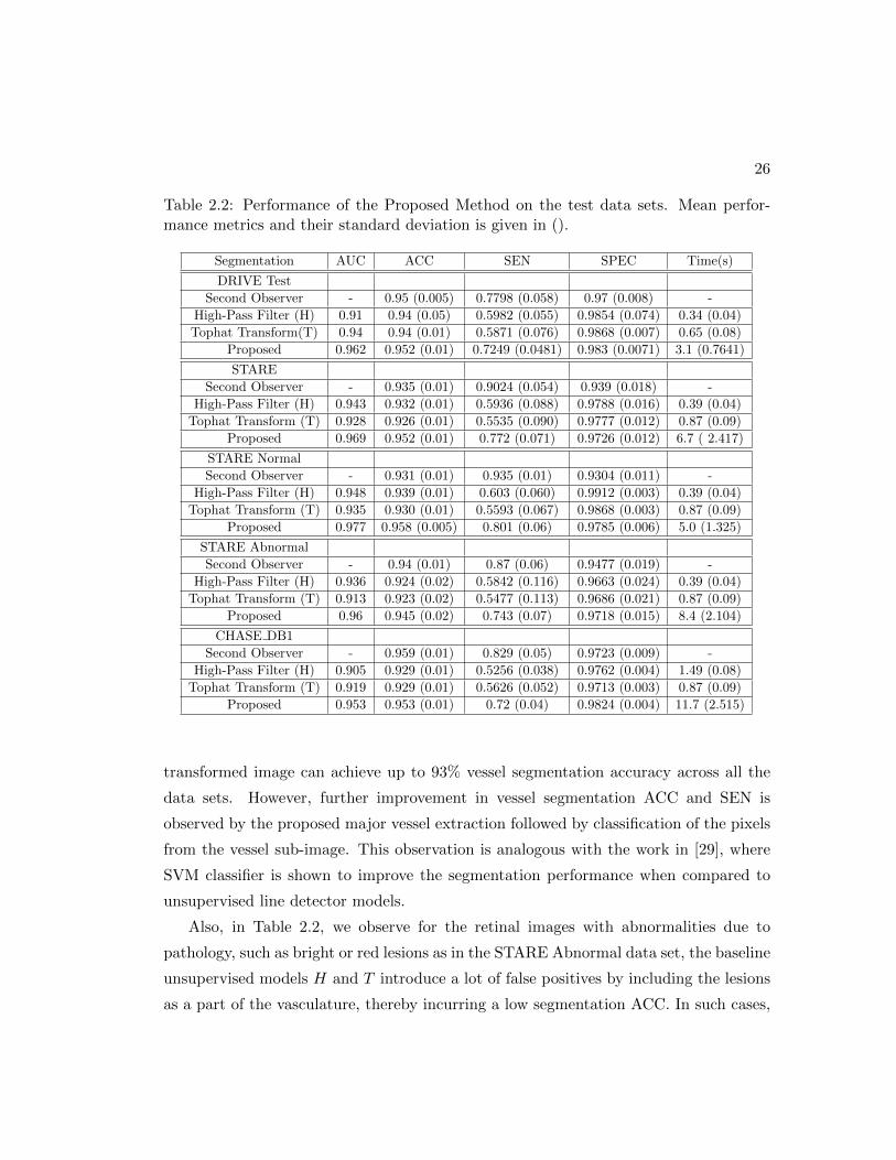
26

Table 2.2: Performance of the Proposed Method on the test data sets. Mean perfor-mance metrics and their standard deviation is given in ().

Segmentation AUC ACC SEN SPEC Time(s)

DRIVE Test

Second Observer - 0.95 (0.005) 0.7798 (0.058) 0.97 (0.008) -

High-Pass Filter (H) 0.91 0.94 (0.05) 0.5982 (0.055) 0.9854 (0.074) 0.34 (0.04)

Tophat Transform(T) 0.94 0.94 (0.01) 0.5871 (0.076) 0.9868 (0.007) 0.65 (0.08)

Proposed 0.962 0.952 (0.01) 0.7249 (0.0481) 0.983 (0.0071) 3.1 (0.7641)

STARE

Second Observer - 0.935 (0.01) 0.9024 (0.054) 0.939 (0.018) -


Tophat Transform (T) 0.928 0.926 (0.01) 0.5535 (0.090) 0.9777 (0.012) 0.87 (0.09)

Proposed 0.969 0.952 (0.01) 0.772 (0.071) 0.9726 (0.012) 6.7 ( 2.417)

STARE Normal

Second Observer - 0.931 (0.01) 0.935 (0.01) 0.9304 (0.011) -



Proposed 0.977 0.958 (0.005) 0.801 (0.06) 0.9785 (0.006) 5.0 (1.325)

STARE Abnormal

Second Observer - 0.94 (0.01) 0.87 (0.06) 0.9477 (0.019) -



Proposed 0.96 0.945 (0.02) 0.743 (0.07) 0.9718 (0.015) 8.4 (2.104)

CHASE DB1

Second Observer - 0.959 (0.01) 0.829 (0.05) 0.9723 (0.009) -



Proposed 0.953 0.953 (0.01) 0.72 (0.04) 0.9824 (0.004) 11.7 (2.515)

transformed image can achieve up to 93% vessel segmentation accuracy across all the

data sets. However, further improvement in vessel segmentation ACC and SEN is

observed by the proposed major vessel extraction followed by classification of the pixels

from the vessel sub-image. This observation is analogous with the work in [29], where

SVM classifier is shown to improve the segmentation performance when compared to

unsupervised line detector models.

Also, in Table 2.2, we observe for the retinal images with abnormalities due to

pathology, such as bright or red lesions as in the STARE Abnormal data set, the baseline

unsupervised models H and T introduce a lot of false positives by including the lesions

as a part of the vasculature, thereby incurring a low segmentation ACC. In such cases,

27

the proposed method first extracts the major vessel regions, followed by classification

of the fine vessel pixels using neighborhood-based and gradient-based features. Large

lesion regions or bright region edges are removed in this classification step and hence,

the proposed approach has higher segmentation ACC than the baseline models.

The images from the CHASE DB1 data set correspond to retinal photographs from

children that are centered at the papilla. These images have deeper pigmentation than

the other data sets that causes false positive pixels to get introduced by the baseline

models. In this case, the proposed method has a superior segmentation ACC due to the

classification of vessel sub-images.

The best and worst vessel segmentation examples from all the three test data sets

are shown in Fig. 2.6. It is noteworthy that the images with the worst segmentation

accuracy in all the three test data sets resemble the manual annotations of the second

human observer more than the first human observer. Since vessel segmentation perfor-

mance is dependent on the manual annotations that are subjective to the observer, the

proposed algorithm performs fairly accurately with respect to both human observers.

Next, the performance and segmentation time of the proposed blood vessel segmen-

tation algorithm in comparison with existing vessel segmentation methods are shown in

Table 2.3.

From Table 2.3, we observe that the proposed vessel segmentation algorithm out-

performs most of the existing methods on the DRIVE Test data set in terms of segmen-

tation ACC and AUC. However, on the STARE data set, the accuracy of the proposed

algorithm is out-performed in terms of ACC and AUC by the existing methods Lam et.

al [21] and Fraz et. al [12]. The method Marin et. al. [13] has better AUC and the

method Ricci et. al. [29] has better ACC. The method by Lam et. al. [21] uses a per-

ceptive transform model to handle abnormal images specifically and incurs considerably

high computational complexity in this process. The method by Fraz et. al. [12] uses

complex decision tree-based classifiers for vessel classification, and hence it suffers from

high computational complexity and test data dependence. The proposed approach of

segmenting the major vessel pixels and fine vessel pixels separately incurs lower com-

putational complexity and consistent segmentation ACC. The method by Marin [13]

trains neural network classifiers on a few hand-picked image pixels from the DRIVE

Train data set and classifies major vessel pixels and fine vessel pixels using the same

28

7-dimensional feature set. Hence, the optimal threshold for vessel-pixel classification

varies significantly with varying FOVs of the test data set, i.e., threshold for DRIVE

Test data set and STARE data sets are 0.63 and 0.91, respectively. Since the proposed

method applies classification for only for the fine vessel pixels, hence the optimal classi-

fication thresholds are observed to be less variable, thereby increasing the robustness of

the proposed method with respect to the existing methods. The method by Ricci et. al.

[29], trains support vector machine (SVM) classifiers using 20,000 manually segmented

randomly chosen pixels from the DRIVE and STARE data set separately. This method

requires SVM classifiers to be retrained for any new test data set and it suffers from

computational complexity due to the SVM classifier.

The proposed method incurs low computational complexity since the major vessels

are extracted by an unsupervised approach followed by supervised identification of fine

blood vessel segments, thereby significantly reducing in the number of pixels under clas-

sification. However, segmentation time is dependent not only on algorithmic complexity

but also on the implementation software and platform. The unsupervised methods by

Budai et. al. (2010) [24] and Budai et. al. (2013) [25] achieve vessel segmentation

in the least time since these methods are implemented using C++ while all the other

methods in Table 2.3 are implemented using MATLAB.

2.4.2 Abnormal Image Analysis

High vessel segmentation performance on abnormal retinal images implies robustness

of the method. To assess the robustness of the proposed method two images from the

STARE Abnormal data set, one with red lesions, and another with bright lesions are

subjected to vessel segmentation using the unsupervised baseline methods (H, T ), and

by the proposed method. The optimal segmentations are shown in Fig. 2.7. These two

abnormal images have been specifically analyzed by some the methods in [19] [20] [21].

The performance of the proposed approach compared to existing segmentation meth-

ods on the two abnormal retinal images in Fig. 2.7 are shown in Fig. 2.8. Using the

proposed method on such retinal images with abnormalities, about 50% of the vessel

pixels are subjected to classification in the vessel sub-image. Small red lesions and

bright lesion edges have similar gradient-based features as the fine vessels, and hence

29

such false edge pixels get classified as vessel pixels, thereby leading to a lower SPEC

when compared to normal retinal images. In Fig. 2.8 (a), we observe that for the image

with red lesions, only the methods by Soares et. al. [28] and Lam et. al. [21] have

better performance than the proposed method. Since the method by Soares et. al. [28]

performs vessel classification by leave-one-out strategy on the images from the STARE

data set, it achieves better segmentation performance than the proposed method. The

method by Lam et. al. [21] is trained specifically for such abnormal images and hence it

has superior segmentation performance. The proposed method outperforms the meth-

ods by Marin et. al. [13], Lam and Yan [20], Hoover et. al. [15], Jiang et. al. [22] and

Vermeer et. al. [19] that include most of the red lesion regions as vessels.

In Fig. 2.8 (b), for the image with bright lesions, we observe that the method Lam et.

al. [21] has better segmentation performance than the proposed method. The methods

by Soares et. al. [28] and Marin et. al. [13] have comparable performance with slightly

less false positives than the proposed approach, but with lower SEN due to the broken

vessel-like structures detected. Thus, we observe that the proposed approach has higher

segmentation accuracy than most existing methods on normal and abnormal retinas

and it is more robust for vessel segmentation when compared to baseline unsupervised

models.

2.4.3 Cross-Training by inter-changing the Training/Test data

The dependence of the proposed segmentation method on the training data set is demon-

strated by interchanging the training and test data sets and analyzing the change in

mean and standard deviation of the vessel segmentation ACC in Table 2.4. As the

training data is changed, the classifier threshold is determined by leave-one out cross

validation on the training set of images. By training on the DRIVE Test, STARE, and

CHASE DB1 data sets, the threshold probabilities were found to be 0.94,0.9 and 0.8,

respectively.

From the second column in Table 2.4, we observe that by training the GMM classifier

on pixels from the STARE and CHASE DB1 data set and testing the classifier on the

DRIVE Test set of images, the mean ACC varies by 0.01% (0.9493 to 0.9494). The

third column demonstrates that by varying the training data set from DRIVE Test to

CHASE DB1 and testing the classifier on STARE set of images, the ACC varies by

30

0.25% (0.951 to 0.9535). The fourth column demonstrates that by varying the training

data set from DRIVE Test to STARE and testing the classifier on the CHASE DB1

image set, the ACC varies by 0.34% (0.9486 to 0.952). Thus, the variation in ACC for

each Test data set by varying the training data set is considerably small, which leads to

low dependence on training data and high robustness of the proposed algorithm. Next,

the performance of cross-training of the proposed algorithm is compared with existing

methods in Table 2.5.

From Table 2.5, we observe that by cross-training, the absolute ACC variations

between DRIVE Test and STARE data sets incurred by the Marin et. al. [13] method,

Ricci et. al. [29] method, Fraz et. al. method [12] and the proposed method are 0.78%,

1.86%, 0.37% and 0.16%, respectively. Also, the absolute ACC variation between the

STARE and CHASE DB1 data set by cross-training is observed to be 0.78% for the Fraz.

et. al. [12] method, and 0.24% for the proposed algorithm. Thus, the segmentation

performance of the proposed method has lower dependence on the training data set when

compared to the existing methods since the segmentation ACC remains significantly

consistent when the training data set is changed.

2.4.4 Peripapillary vessel analysis

In retinal fundus images, the blood vessels in and around the optic disc are referred to

as the peripapillary blood vessels. Many retinal abnormalities such as proliferative DR

(PDR), glaucoma, central retinal vein occlusion, cilio retinal artery occlusion can lead

to changes in the blood vessel structure mainly in the peripapillary region. For instance,

neovascularization at the disc (NVD) caused due to PDR is evident if new blood vessels

are visible within 1-optic disc diameter (1-DD) centered at the papilla [34]. For this

purpose, the images from the DRIVE, STARE and CHASE DB1 data set were manually

annotated for the optic disc boundary and optic nerve head in each image, and then,

a mask was created centered at the optic nerve head with 1-DD radius to extract the

peripapillary region. The first 19 images from the STARE vessel segmentation data set

contain the peripapillary region and hence peripapillary vessel detection was performed

on these 19 images only.

The segmented vessel images using the Marin et. al. method [13]1 , Soares et.

1 Available at http://www.uhu.es/retinopathy/eng/bd.php

31

al. method [28] 2 , Jiang et. al. method [22] and Staal et. al. method [27] 3 are

downloaded from the respective websites for comparison. Next, the performance of

the proposed vessel segmentation method in comparison with existing methods and the

more detailed second human observer annotations for the STARE data set is shown

in Fig. 2.9. The segmented vessel images are compared to the segmentation results

produced by the Marin et. al. method [13], Soares et. al. method [28] and Hoover et.

al. method [15] 4 . We observe that the proposed method has a better accuracy for

segmenting the peripapillary vessels for both these blood vessels.

Finally, we compute the performance of peripapillary vessel segmentation for the

three data sets with respect to the two human observers in Table 2.6. We observe

that for the DRIVE Test data set, the proposed segmentation algorithm results in 0.1%

(with respected to Marin et. al. [13]) to 6.1% (with respected to Jiang et. al. [22])

improvement in vessel accuracy when compared to existing methods using the first

human observer annotations, and 0.8% to 7.0% improvement against the same methods

using the second human observer.

For the STARE data set, the proposed vessel segmentation achieves 3.3% (with

respected to Marin et. al. [13]) to 8.2% (with respected to Hoover et. al. [15])

improvement in vessel accuracy when compared to existing methods using the first

human observer annotations, and 4.5% (with respected to Soares et. al. [28]) to 5.4%

(with respected to Hoover et. al. [15]) improvement using the second human observer.

For the CHASE DB1 data set, peripapillary vessel segmentation accuracy greater than

83% is achieved with respect to both human observers.

2.5 Discussion and Conclusions

The most important feature of the proposed segmentation algorithm is separate seg-

mentation of major vessel and fine vessel regions. Major vessels regions are identified

as the intersecting regions between thresholded versions of two pre-processed images,

i.e., the high-pass filtered image and tophat transformed image. The pixel threshold ‘p’

2 Available at http://sourceforge.net/apps/mediawiki/retinal/index.php?title=Segmentation results

3 Available at http://www.isi.uu.nl/Research/Databases/DRIVE/browser.php4 Available at http://www.parl.clemson.edu/ ahoover/stare/probing/index.html

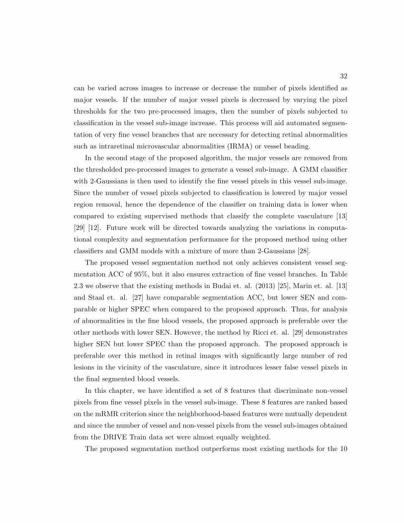
32

can be varied across images to increase or decrease the number of pixels identified as

major vessels. If the number of major vessel pixels is decreased by varying the pixel

thresholds for the two pre-processed images, then the number of pixels subjected to

classification in the vessel sub-image increase. This process will aid automated segmen-

tation of very fine vessel branches that are necessary for detecting retinal abnormalities

such as intraretinal microvascular abnormalities (IRMA) or vessel beading.

In the second stage of the proposed algorithm, the major vessels are removed from

the thresholded pre-processed images to generate a vessel sub-image. A GMM classifier

with 2-Gaussians is then used to identify the fine vessel pixels in this vessel sub-image.

Since the number of vessel pixels subjected to classification is lowered by major vessel

region removal, hence the dependence of the classifier on training data is lower when

compared to existing supervised methods that classify the complete vasculature [13]

[29] [12]. Future work will be directed towards analyzing the variations in computa-

tional complexity and segmentation performance for the proposed method using other

classifiers and GMM models with a mixture of more than 2-Gaussians [28].

The proposed vessel segmentation method not only achieves consistent vessel seg-

mentation ACC of 95%, but it also ensures extraction of fine vessel branches. In Table

2.3 we observe that the existing methods in Budai et. al. (2013) [25], Marin et. al. [13]

and Staal et. al. [27] have comparable segmentation ACC, but lower SEN and com-

parable or higher SPEC when compared to the proposed approach. Thus, for analysis

of abnormalities in the fine blood vessels, the proposed approach is preferable over the

other methods with lower SEN. However, the method by Ricci et. al. [29] demonstrates

higher SEN but lower SPEC than the proposed approach. The proposed approach is

preferable over this method in retinal images with significantly large number of red

lesions in the vicinity of the vasculature, since it introduces lesser false vessel pixels in

the final segmented blood vessels.

In this chapter, we have identified a set of 8 features that discriminate non-vessel

pixels from fine vessel pixels in the vessel sub-image. These 8 features are ranked based

on the mRMR criterion since the neighborhood-based features were mutually dependent

and since the number of vessel and non-vessel pixels from the vessel sub-images obtained

from the DRIVE Train data set were almost equally weighted.

The proposed segmentation method outperforms most existing methods for the 10

33

abnormal retinal images with pathology in the STARE Abnormal data set as shown

in Table 2.7. The method by Marin et. al. [13], Lam and Yan [20] and Lam et. al.

[21] have higher segmentation ACC or AUC than the proposed method, but they incur

higher computational complexity as compared to the proposed approach.

The next most significant feature of the proposed method is the high accuracy of

peripapillary blood vessel extraction that makes the proposed segmentation algorithm

very useful for computer-aided screening for patients with PDR, glaucoma and retinal

vein occlusions.

The low computational complexity and low dependence on training data make the

proposed algorithm ideal for integration with retinal screening systems. Future work

will be directed towards combining the proposed algorithm with DR screening systems

such as [3] to detect neovascularization in the peripapillary region, and to reduce false

positives while detecting red lesions. Also, the proposed method will be further fine-

tuned for automated extraction of vessels in wide-field fundus images with 200o FOV.

34

Figure 2.6: Best and worst vessel segmentation examples from the DRIVE Test, STARE,and CHASE DB1 data sets. (a) Original image. (b) first human observer annotation.(c) second human observer annotation. (d) Segmented vessels using the proposed algo-rithm. In the images with worst ACC, the segmented vessels within the region enclosedby the green circle resemble the manual annotations of the second human observer morethan the first human observer.

35

Table 2.3: Comparative Performance of Proposed Model with existing works on theDRIVE and STARE data sets.

Test Data: DRIVE Test

Method ACC SPEC SEN AUC Time

Jiang et. al. [22] 0.891 0.90 0.83 0.932 8-36 s

Niemeijer et. al. [26] 0.942 0.969 0.689 0.93 -

Staal et. al. [27] 0.944 0.977 0.719 0.952 15 mins

Mendonca et. al. [17] 0.945 0.976 0.734 - 2.5 mins

Soares et. al. [28] 0.946 0.978 0.733 0.961 ∼3 mins

Ricci et. al. [29] 0.959 0.972 0.775 0.963 -

Al-Diri et. al.[23] - 0.955 0.728 - 11 mins

Lam et. al. [21] 0.947 - - 0.961 13 mins

Budai et. al.(2010)[24] 0.949 0.968 0.759 - 11 s

Budai et. al. (2013) [25] 0.9572 0.987 0.644 - 1.04s

Marin et. al. [13] 0.945 0.98 0.706 0.958 ∼90 s

Miri et.al. [18] 0.943 0.976 0.715 - ∼50 s

Fraz et. al. [12] 0.948 0.981 0.74 0.974 ∼100 s

Proposed 0.952 0.983 0.725 0.962 3.11 s

Test Data: STARE

Hoover et. al. [15] 0.927 0.81 0.65 0.75 5 mins

Jiang et. al. [22] 0.901 0.90 0.857 0.929 8-36 s

Staal et. al. [27] 0.952 0.981 0.697 0.961 15 mins

Mendonca et. al. [17] 0.944 0.973 0.699 - 3 mins

Soares et. al. [28] 0.948 0.975 0.72 0.967 ∼3 mins

Ricci et. al. [29] 0.965 0.939 0.903 0.968 -

Lam and Yan [20] 0.9474 - - 0.9392 8 mins

Al-Diri et. al.[23] - 0.968 0.752 - -

Lam et. al. [21] 0.957 - - 0.974 13 mins

Budai et. al.(2010)[24] 0.938 0.975 0.651 - 16 s

Budai et. al. (2013) [25] 0.9386 0.982 0.58 - 1.31s

Marin et. al. [13] 0.952 0.982 0.694 0.977 ∼90 s

Fraz et. al. [12] 0.953 0.976 0.755 0.976 ∼100 s

Proposed 0.951 0.973 0.772 0.969 6.7 s

36

Figure 2.7: Vessel segmentation on abnormal images. First row depicts vessel segmenta-tion on an image with red lesions while the second row depicts segmentation on an imagewith bright lesions. (a) Image (b) Manually marked vessels. (c) Thresholded tophattransformed image (T > 0.44). (d) Thresholded high-pass filtered image (H > 0.36).(e) Major vessels detected (P ). (f) Final segmented vasculature using proposed method.

Table 2.4: Vessel Classification ACC by Cross-Training.Train Data Test Data

DRIVE Test STARE CHASE DB1

DRIVE Test NA 0.951 (0.013) 0.952 (0.005)

STARE 0.9494 (0.0072) NA 0.9486 (0.011)

CHASE DB1 0.9493 (0.0071) 0.9535 (0.016) NA

Table 2.5: Segmentation Performance with Cross Training in terms of mean ACC givenfor Test Data (Training data).

Method DRIVE Test STARE CHASE DB1(STARE) (DRIVE Test) (STARE)

Marin et al. [13] 0.9448 0.9526 -

Ricci et al. [29] 0.9266 0.9452 -

Fraz et. al. [12] 0.9456 0.9493 0.9415

Proposed 0.9494 0.951 0.9486

37

(a)

(b)

Figure 2.8: Comparative performance of existing methods with proposed method on theabnormal retinal images. (a) ROC curve for the first abnormal image with red lesionsin Fig. 2.7. (b) ROC curve for the second abnormal image with bright lesions in Fig.2.7.

38

Figure 2.9: Peripapillary vessels segmented for the STARE set of images. (a) SecondHuman Observer. (b) Marin et. al. method. (c) Soares et. al. method, (d) Hoover et.al. method. (e) Proposed Method.

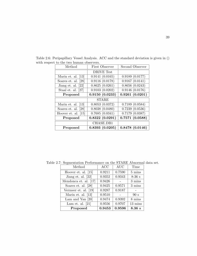
39

Table 2.6: Peripapillary Vessel Analysis. ACC and the standard deviation is given in ()with respect to the two human observers.

Method First Observer Second Observer

DRIVE Test

Marin et. al. [13] 0.9141 (0.0165) 0.9189 (0.0177)

Soares et. al. [28] 0.9116 (0.0178) 0.9167 (0.0141)

Jiang et. al. [22] 0.8625 (0.0261) 0.8656 (0.0243)

Staal et. al. [27] 0.9103 (0.0202) 0.9146 (0.0176)

Proposed 0.9150 (0.0233) 0.9261 (0.0201)

STARE

Marin et. al. [13] 0.8053 (0.0372) 0.7189 (0.0584)

Soares et. al. [28] 0.8038 (0.0480) 0.7239 (0.0536)

Hoover et. al. [15] 0.7685 (0.0341) 0.7179 (0.0387)

Proposed 0.8322 (0.0291) 0.7571 (0.0588)

CHASE DB1

Proposed 0.8393 (0.0205) 0.8478 (0.0146)

Table 2.7: Segmentation Performance on the STARE Abnormal data set.Method ACC AUC Time

Hoover et. al. [15] 0.9211 0.7590 5 mins

Jiang et. al. [22] 0.9352 0.9343 8-36 s

Mendonca et. al. [17] 0.9426 - 3 mins

Soares et. al. [28] 0.9425 0.9571 3 mins

Vermeer et. al. [19] 0.9287 0.9187 -

Marin et. al. [13] 0.9510 - 90 s

Lam and Yan [20] 0.9474 0.9392 8 mins

Lam et. al. [21] 0.9556 0.9707 13 mins

Proposed 0.9453 0.9596 8.36 s

Chapter 3

Automated Vessel Segmentation:

An Iterative Algorithm

3.1 Introduction

Retinal blood vessel (vasculature) segmentation using fundus photographs has played

a vital role in assessing the severity of retinal pathologies that can lead to acquired

blindness such as retinopathy of prematurity [35], glaucoma, vein occlusions and dia-

betic retinopathy (DR) [36]. According to research statistics in the year 2011, retinal

pathologies such as DR affect over 4.2 million Americans each year, while glaucoma

affects about 2.3 million Americans annually [5]. In such a scenario, automated blood

vessel segmentation algorithms can be very useful in screening patients that are affected

by such retinal complications and require follow-up [4]. Also, automated blood ves-

sel segmentation systems can be useful in determining variations in the blood vessels

based on the vessel branching patterns, vessel width, tortuosity and vessel density as the

pathology progresses in patients [6]. Such evaluations will help to enhance the resource-

fulness of the present-day retinal therapeutics and guide research towards analyzing

patients for hypertension [7], variability in retinal vessel diameters due to a history of

cold hands and feet [8], and flicker responses [9].

Some existing automated detection systems for non-proliferative DR detection, such

as [10] [3] [37], require masking of the blood vessels to ensure that the blood vessels

are not mistaken for red lesions that are caused by DR. Additionally, proliferative DR

40

41

detection systems [34] require analysis of the vessel parameters for detecting neovas-

cularization, vessel beading and intra retinal micro-vascular abnormalities (IRMA). A

fast and accurate segmentation algorithm for detecting the blood vessels is necessary

for such automated real-time detection and screening systems. In this chapter, we pro-

pose an unsupervised vasculature segmentation algorithm that iteratively estimates the

blood vessels with significantly high accuracy in normal images as well as images with

abnormalities such as bright lesions like exudates or red lesions like hemorrhages or

micro-aneurysms. After an initial training with any arbitrary data set, this novel ap-

proach does not require any retraining on new datasets and is robust to variations in the

fundus image fields of view (FOV), uneven illumination, pigmentation and pathology.

Additionally, the proposed algorithm is computationally the fastest and most consistent

in segmentation performance across the three data sets of DRIVE [27], STARE [15] and

CHASE DB1 [30].

Key contributions of the chapter include a novel iterative blood vessel segmentation

algorithm, where vasculature estimates are identified by adding new pixels iteratively

using adaptive global thresholding, and a novel stopping criterion to terminate the

iterative vessel addition process thereby reducing the number of false edge pixels in

the segmented image. The proposed vessel segmentation algorithm is robust to image

variability, achieves high segmentation accuracy in normal as well as abnormal retinal

images. For the images in STARE data set, the proposed approach achieves an average

accuracy of 95.6%. We identify vessel segmentation accuracy in the peripapillary region

as another important metric; this metric is well suited for images with abnormalities

such as proliferative DR, glaucoma and retinal occlusions. The peripapillary blood

vessels contain vessels within 1-optic disc diameter centered at the papilla [34]. It is

shown that the proposed approach provides the highest vessel segmentation accuracy

in the peripapillary region among all known algorithms.

The organization of this chapter is as follows. In Section 3.2, the prior automated

vessel segmentation algorithms in the literature are reviewed. The proposed method

and materials are described in Section 3.3. In section 3.4, the experimental results

are presented and compared with existing methods, for normal and abnormal retinal

images, and for peripapillary vessel extraction. Finally, in Section 3.5, discussion and

significant conclusions are presented.

42

3.2 Prior Work

All existing algorithms for automated segmentation of blood vessels using fundus images

can be broadly categorized as supervised and unsupervised methods. The methods

belonging to these categories are explored below.

The supervised vessel segmentation algorithms classify pixels as vessel and non-

vessel. One such method in [26] trains the k-Nearest Neighbor classifier with 31-features

extracted using Gaussians and its derivatives of the fundus image. This method was

further improved in [27] by applying ridge-based vessel detection, where each pixel is

assigned to its nearest ridge element, thus partitioning the image. For classification, 27

features corresponding to each pixel are computed, followed by kNN classification. These

methods are computationally intensive due to the large size of the classification feature

sets. Other methods with smaller classification features include a Gaussian Mixture

Model (GMM) classifier where 6-features are extracted using Gabor-wavelets for vessel

classification [28]. This method is also computationally intensive since it requires several

hours for training GMM models with a mixture of 20 Gaussians. Another method in

[29] uses line operators and a support vector machine (SVM) classifier with 3-features

per pixel for classification. The method in [13] applies neural network classifiers using

7-features extracted by neighborhood parameters and moment invariants-based method.

Also, the method in [12] applies boosting and bagging strategies with 200 decision trees

and 9-features for vessel classification extracted by Gabor filters. This method suffers

from high computational complexity as well due to the boosting strategy. All these

supervised vessel classification-based methods are dependent on the training data and

sensitive to false edges as well.

Among the existing unsupervised methods, algorithms that apply matched filtering,

vessel tracking, morphological transformations and model-based algorithms are predom-

inant. In the matched filtering-based method in [15], a 2-D linear structuring element is

used to extract Gaussian intensity profiles of the blood vessels. The structuring element

is rotated 8-12 times to fit the vessels in different configurations to extract the vessel

boundaries. This method has a high time complexity since a stopping criterion needs to

be evaluated for each end pixel. A morphology-based method in [17] combines morpho-

logical transformations with curvature information and matched-filtering for detecting

43

the central line of the blood vessels. This method is sensitive to false edges introduced by

bright region edges such as optic disc and exudates. Another morphology based method

in [18] uses multiple structuring elements to extract vessel ridges followed by connected

component analysis. In another model-based method [19], blood vessel structures are

extracted by convolving with a Laplacian kernel followed by thresholding and connect-

ing broken line components. An improvement of this methodology was presented in [20],

where the blood vessels are extracted by the Laplacian operator and noisy objects are

pruned according to center lines. This method focuses on vessel extraction from images

with bright abnormalities, but it does not perform very effectively on retinal images

with red lesions (such as hemorrhages or microaneurysms). The method in [21] presents

perceptive transformation approaches to segment vessels in retinal images with bright

and red lesions. A model-based method in [22] applies locally adaptive thresholding

and incorporates vessel information into the verification process. Although this method

is more generalizable than matched-filter based methods, it has a lower overall vessel

segmentation accuracy. Another model-based vessel segmentation approach proposed in

[23] uses active contour models. Additionally, a multi-scale vessel segmentation method

proposed in [24] uses neighborhood analysis at each level of a 3-level Gaussian pyramid.

All these unsupervised methods are computationally complex and hence they are not

viable for real-time portable DR screening systems such as [3]. Most of the unsupervised

approaches such as [28], [20] perform well on healthy retinal images but have low seg-

mentation accuracy in images with pathology. Also, methods like [17] [21] have higher

segmentation accuracy on pathological images than most other methods. Thus, there

is a need for a general method that produces high segmentation accuracy for normal as

well as pathological fundus images.

In this chapter, we propose an iterative vessel segmentation algorithm that segments

the major vessels first, followed by addition of finer vessel branches by adaptive thresh-

olding in iterative steps. A novel stopping criterion is designed to estimate the best

segmented vessel estimate such that the algorithm stops before false positive pixels, due

to uneven illumination or pigmentation, or edges of bright lesions, optic disc or red

lesions, get added to the segmented vessel estimate. This iterative approach has high

segmentation accuracy for vasculature in normal and abnormal retinal images. Also,

the proposed method has lower computational complexity than all existing supervised

44

and unsupervised approaches.


The principal idea behind iterative vessel segmentation is that in a vessel enhanced

image, the bright and large vessels overshadow the thinner fine vessel branches. In such

a situation, global thresholding would extract only the large prominent vessels while the

finer vessel branches would remain unsegmented. Thus, to include these fine vessels into

the segmented vasculature estimate, iterative adaptive global thresholding is proposed.

For every color fundus photograph, a vessel enhanced image is obtained by morpho-

logical tophat reconstruction of the negative green plane image. The brightest pixels

from this vessel enhanced image are extracted as the major portions of the vascula-

ture, or major vessels. A residual image is then generated by masking these major

vessels from the vessel enhanced image followed by contrast adjustment and adaptive

thresholding in an iterative manner to uncover new vessel pixels and add them to the

existing vessel estimate. This method of iterative vessel addition and a novel stopping

criterion for estimating the best segmented vasculature is presented in this section. The

segmentation performance of the proposed algorithm is evaluated using three publicly

available data sets with different resolutions and FOVs. The proposed algorithm has

been implemented in MATLAB environment on a Laptop with Intel Core i3 processor,

2.6GHz and 2GB RAM.

3.3.1 Data

The following data sets have been manually annotated for the blood vessel regions for

analyzing the performance of blood vessel segmentation algorithms.

• STARE [15] data set contains 20 images with 35o FOV of size [605x700] pixels that

are manually annotated by two independent human observers. Here, 10 images

represent patients with retinal abnormalities (STARE Abnormal). The other 10

images represent normal retina (STARE Normal).

• DRIVE [27] data set contains 40 images with 45o FOV of size [584x565] pixels.

This data set is separated by its authors into a training set (DRIVE Train) and

45

a test set (DRIVE Test) with 20 images in each set. The DRIVE Train set of

images are annotated by one human observer while the DRIVE Test data set is

annotated by two independent human observers.

• CHASE DB1 [30] data set contains 28 images with 30o FOV of size [960x999] pixels

corresponding to two images per patient (one image per eye) for 14 children. Each

image is annotated by two independent human observers [12].

3.3.2 Proposed Method

As a pre-processing stage, the green plane of each fundus image is scaled in [0,1] (I). A

fundus mask (g) is utilized to remove the dark background region from the photographs

to focus attention on the retinal region only. The fundus masks for DRIVE, STARE

and CHASE DB1 data sets are generated as centered elliptical regions with diameters

of [521x520], [550x650] and [860x869] pixels, respectively.

In the scaled green plane image (I), the red regions corresponding to the blood vessel

segments appear as dark pixels with intensities close to 0. To focus attention on the

blood vessel regions, image I is inverted to make the red regions appear the brightest,

followed by superposition of the mask g, resulting in image Iv. Iv is then subjected

to contrast enhancement followed by morphological tophat transformation. 12 linear

structuring elements each of length 21 pixels and 1 pixel width and angles incremented

by 15o from 0 through 180o are used to generate tophat reconstructions from Iv [17] [12].

The length of 21 pixels for the linear structuring element is chosen to approximately

fit the diameter of the biggest vessels in the images [12]. For each pixel location, the

reconstructed pixel with the highest intensity is selected, thereby resulting in tophat

reconstructed vessel enhanced image T .

The major vessels (V0) are extracted by thresholding image T for pixels greater

than 0.5, and retaining the regions with area greater than 200 pixels. Thus, V0 is

the segmented vessel estimate (Vt) at iteration t = 0. Next, the following steps are

iteratively performed:

For each iteration t, the pixels from the existing vessel estimate Vt are removed

from image T and the remaining image is contrast enhanced resulting in residual image

Rt. This image Rt is thresholded at pixel value φ1(t) to extract a binary image VRt

46

containing new vessel regions that have an area of at least 10 pixels. Here, the pixel

threshold value φ1(t) varies with ‘t’, the iteration number. However, it is desirable for

the segmented vessel to have a continuous structure and hence it is imperative to fill

any gaps or holes between the existing vessel estimate Vt and the newly identified vessel

pixels in VRt . Thus, the pixels in Vt and VRt are added to vessel enhanced image T ,

followed by rescaling the pixels in [0,255], resulting in base image Bt. This image Bt is

then region-grown with a threshold pixel value (φ2(t)) that is a function of the iteration

number. The image obtained at the end of the regiongrow operation [38] is the new

iterative vessel estimate (Vt+1).

The iterative addition of the newly identified vessel regions to the existing vessel

estimate is continued till a stopping criterion is met. The notations and their definitions

used in this iterative algorithm are defined in Table 3.1.

For an image from the DRIVE data set, the iterative vessel estimates are shown in

Fig. 3.1 for 10 iterations, i.e., t = [1, 2...10]. The proposed iterative segmentation algo-

rithm is given in Algorithm 1. For the example shown in Fig. 3.1, the best segmented

vasculature is estimated at iteration t = 4.

For post-processing, the regions in the best vessel estimate with area less than 20

pixels are discarded, and the remaining vessel regions are median filtered with a [3x3]

filter.

It is important to note that Algorithm 1 relies on two threshold parameters that

impact the accuracy of the final vessel estimate. These two threshold parameters φ1(t)

and φ2(t) affect the quality of new vessel pixels that are added to the existing vessel

estimate. The other important feature in the iterative vessel segmentation algorithm

is the estimation of the iteration number (tf ) at which the best vessel estimate with

the highest segmentation accuracy occurs. To determine tf , a stopping criterion is

introduced. The methods for estimating the adaptive thresholds φ1(t) and φ2(t), and

stopping criterion are given below.

Thresholds for vessel addition

In each iteration step ‘t’, new vessels are identified from the iterative residual image in

VRt using pixel threshold φ1(t). Here, we initialize φ1(t) = 1−(0.05∗t). As the algorithm

progresses to combine the new vessel pixels (VRt) to the existing vessel estimate (Vt), a

47

Algorithm 1 Iterative Vessel Segmentation (I, g)

Input: I ∈ [0, 1], g ∈ [0, 1]Output: VfPre-Processing:

Iv ← contrast adjust((1− I) g)T ← tophat reconstruction(Iv)V0 ← [(T > 0.5), and area > 200]

Iterations:t = 0, stop← ‘No’, stop ∈ [‘Yes’,‘No’],

while [stop← ‘No’ ] do∀(i, j), Rt(i, j) = [T (i, j)− Vt(i, j)]|Rt(i, j) ≥ 0.VRt ← [Rt > φ1(t), and area > 10]Bt ← scale (VRt ∪ Vt+ T ∈ [0, 255])Vt+1 ← regiongrow(Bt, seed=255, threshold=φ2(t))t← t+ 1stop ← Stopping criterion (Vt, Vt−1)

end whiletf ← tVf ← Vtfreturn Vf

regiongrow operation [38] is performed by scaling the image (VRt ∪ Vt) + T in [0,255],

using a seed pixel value of 255, and a threshold pixel value φ2(t). The threshold function

φ2(t) that would result in significantly high accuracy for vessel segmentation is obtained

by one-time training using the 20 images from the DRIVE Train data set. We consider

φ2(t) given by:

φ2(t) = 205 + α ∗ (t− 1)k, α ∈ [1, 2...6], k ∈ [0, 0.2, ...3] (3.1)

Each of the 20 images were subjected to vessel segmentation for all the 6x16 com-

binations of ‘α’ and ‘k’ values in (3.1) and [t = 1, 2..10] iterations. For every image

(l = [1...20]), and for each combination of [α, k], the highest segmentation accuracy

(ACC l) was achieved at iteration number tl. The mean ACC l and the corresponding

mean tl versus [α, k] are shown in Fig. 3.2 (a) and Fig. 3.2 (b), respectively. Since,

a low mean iteration number implies higher segmentation speed for the algorithm, the

goal was to select a threshold function that generates the highest mean vessel segmen-

tation accuracy in less iterations. We observe that, the highest mean ACCl occurs for

48

α = 1, k = 1.8, with the mean iteration number tl = 4. Thus, the threshold function

φ2(t) for Algorithm 1 was estimated as φ2(t) = 205 + (t− 1)1.8.

Stopping criterion design

In Fig. 3.1, we observe that the best vessel estimate occurs at some iteration between

t = 0 to t = 10. Also, Algorithm 1 requires a stopping criterion to stop the iterative

vessel addition process at iteration number tf where a segmentation vasculature with

highest accuracy exists. This stopping criterion can be determined by analyzing the

quality of segmented vessel estimates in every iteration.

The initial vessel segment V0 contains the major portions of the blood vessels and

hence it is free from false edge pixels. In each iteration, new pixels are added to the

existing blood vessels. While actual vessel pixels are added in each iteration, pixels cor-

responding to false edges also get introduced into the segmented vessel structure. Using

the manually marked vessels V and the iterative vessel estimate Vt in each iteration

t, the criteria for any pixel (i, j) to be a true positive (tpt), true negative (tnt), false

positive (fpt) and false negative (fnt) are defined in (3.2)-(3.5). The total number of

pixels that are true positives (TPt), true negatives (TNt), false positives (FPt) and false

negatives (FNt) in each image are then computed using (3.6)-(3.9).

49

For the binary image Vt, in iteration t we define: (3.2)

∀(i, j), i ∈ [1, 2...n1], j ∈ [1, 2....n2],

tpt(i, j) = 1, if, [V (i, j) = 1, Vt(i, j) = 1].

tnt(i, j) = 1, if, [V (i, j) = 0, Vt(i, j) = 0]. (3.3)

fpt(i, j) = 1, if, [V (i, j) = 0, Vt(i, j) = 1]. (3.4)

fnt(i, j) = 1, if, [V (i, j) = 1, Vt(i, j) = 0]. (3.5)n1∑i=1

n2∑j=1

tpt(i, j) = TPt,

n1∑i=1

n2∑j=1

tnt(i, j) = TNt, (3.6)

n1∑i=1

n2∑j=1

fpt(i, j) = FPt,

n1∑i=1

n2∑j=1

fnt(i, j) = FNt. (3.7)

The sum of all pixels in binary image Vt represents

the total number of TPt and FPt pixels in Vt.

⇒n1∑i=1

n2∑j=1

Vt(i, j) = TPt + FPt. (3.8)

Also, n1 · n2 = TPt + TNt + FPt + FNt. (3.9)

For a fundus image with [n1 · n2] pixels, the metrics identifying the quality of seg-

mented vessel (Qt), the change in vessel estimate Ct and error in the vessel estimate Et,

are defined in (3.10) - (13). In (12), we observe that Et has two non-zero components,

one due to the FNt pixels and the other due to FPt pixels. The vessel segmentation

accuracy ACCt increases as Et decreases as described by (13). Thus, the iteration tf

corresponding to minimum Etf will ensure a segmented vessel estimate with highest

accuracy.

50

Define :Qt =

∑n1i=1

∑n2j=1[tpt(i, j)]∑n1

i=1

∑n2j=1[fpt(i, j)]

=TPtFPt

. (3.10)

Ct =1

n1 · n2

n1∑i=1

n2∑j=1

Vt(i, j)− V0(i, j) . (3.11)

Et =1

n1 · n2

n1∑i=1

n2∑j=1

|V (i, j)− Vt(i, j)|. (3.12)

⇒ Et =

∑n1i=1

∑n2j=1[fpt(i, j) + fnt(i, j)]

TPt + TNt + FPt + FNt= 1−ACCt. (3.13)

Intuitively, Ct can be modeled as an odd-degree polynomial, and Et can be modeled

as an even-degree polynomial. The goal of segmentation is to stop at the iteration

with least error to maximize the vessel segmentation accuracy. However, Et requires

knowledge of the manual annotated image and is not known. Therefore, Et cannot be

used as a parameter in the stopping criteria. However, an analysis of the trends in Ct

and Et based on known images demonstrates a correlation between these parameters.

This allows us to derive a stopping criterion using Ct. Later in the section we propose

to stop the iterations when the first three derivatives of Ct are non-negative. This is

illustrated in Fig. 3.3. A key contribution of this chapter is that stopping criterion does

not depend on the imaging parameters such as field of view.

To understand the trends of the curves Ct and Et, we consider a theoretical example

shown in Fig. 3.4, where curves Cx and Ex are odd and even functions of the same

repeated root, respectively. In Fig. 3.4, Ex is a function of 4th degree repeated root,

and hence we analyze the trends of the first three derivatives of Ex and Cx computed

using backward difference rule as ‘x’ varies from [1 to 20] in intervals of 1. We observe

that although Ex and Cx are both functions of repeated roots at x = 10.5, the first three

derivatives of both Ex and Cx become non-negative, i.e., [E1x, E

2x, E

3x] ≥ 0, [C1

x, C2x, C

3x] ≥

0 for [x ≥ 12]. The region from x = 9 to x = 12 has very small variations in Cx

and Ex and hence the major variations in the curve trends is observed only beyond

x = 12. Also, we observe that in Fig. 3.4, three significant regions exist corresponding

to high, medium and low quality of segmented vessel pixels (Q). The region with high Q

corresponds to the early iterations when the number of actual vessel pixels identified are

51

more than the noisy false edge pixels (TPt >> FPt). The region with low Q corresponds

to iterations when the number of false edge pixels being added exceed the actual vessel

pixels (TPt << FPt). The third significant region is when Q is medium and change in

iterative vessel estimates is significantly small.

The trends of the C and E curves in the regions when Q is high and Q is low are

analyzed in (3.14)-(3.16). We observe that, curve Ct always has a non-decreasing trend

(15).

Ct+1 − Ct =1

n1 · n2

n1∑i=1

n2∑j=1

Vt+1(i, j)− Vt(i, j) , (3.14)

Since new vessel pixels are added in each iteration,n1∑i=1

n2∑j=1

Vt+1(i, j) ≥n1∑i=1

n2∑j=1

Vt(i, j)⇒ Ct+1 − Ct ≥ 0. (3.15)

⇒ Ct always has non− decreasing trend.

Now, Et+1 − Et =1

n1 · n2

n1∑i=1

n2∑j=1

[|V (i, j)− Vt+1(i, j)|

−|V (i, j)− Vt(i, j)|],

⇒ Using (12), Et+1 − Et =1

n1 · n2

n1∑i=1

n2∑j=1

[fpt+1(i, j)

+fnt+1(i, j)− fpt(i, j)− fnt(i, j)]. (3.16)

However, for Et, we consider two separate cases to analyze the trends of Et in high Q

and low Q regions. In case 1 with high Q, TPt >> FPt. Here, the number of false vessel

pixels in Vt (FPt) are very small compared to the number of true vessel pixels (TPt)

added in consecutive iterations (3.17). Also, for each image, the sum of vessel pixels

in the manually marked image remains constant, i.e., TPt + FNt = constant (3.18).

Hence in the high Q region, Et has a non-increasing trend (3.19). In case 2 with low Q,

TPt << FPt. Here, the number of false vessel pixels in Vt (FPt) are significantly larger

than the true vessel pixels (TPt) (3.20). We observe that Et has a non-decreasing trend

in this region (3.21). Thus, to achieve the most accurate segmented vessel estimate, the

iteration process must be stopped in the transition region from high Q to low Q.

52

Case 1: High Q, [TPt << FPt].

Iteratively, TPt+1 ≥ TPt, FPt+1 ≈ FPt. (3.17)

⇒ TPt + FNt =

n1∑i=1

n2∑j=1

V (i, j) = constant. (3.18)

Using, (17), (18), FNt+1 ≤ FNt.

From (16), ⇒ Et+1 − Et ≤ 0.

⇒ Et has non− increasing trend. (3.19)

Case 2: Low Q, [TPt << FPt].

Iteratively, FPt+1 ≥ FPt, TPt+1 ≈ TPt (3.20)

⇒ FNt+1 ≈ FNt.

From (16), ⇒ Et+1 − Et ≥ 0.

⇒ Et has non− decreasing trend. (3.21)

From the experimental standpoint, for an image from the DRIVE Test data set, the

curve E and C as iterations proceed from t = 0 to t = 10 are shown in Fig. 3.5. Here,

we observe that the best fit polynomial for C is of degree 3 and the best fit polynomial

for E is of degree 4. Thus, the first, second and third derivatives must exist for both

curves C and E. Let these derivatives be denoted by Cmt and Emt , for m = [1, 2, 3],

respectively. These derivatives are computed iteratively using the backward difference

rule as shown in (3.22).

If, C0t = Ct, E

0t = Et, then, (3.22)

Emt = Em−1t − Em−1

t−1 ,m = [1, 2, 3].

Cmt = Cm−1t − Cm−1

t−1 ,m = [1, 2, 3].

Further, from Fig. 3.4, we observe that the iterative change in Ct and Et are signifi-

cantly small in the medium Q region than the high and low Q regions. This is intuitive

53

since in the medium Q region, fine vessel branches are detected and added to the existing

vessel estimate. However, as soon as the noisy false edge regions, that are significantly

larger in area when compared to the fine vessel branches, start getting identified and

added to the vessel estimates, the change in Ct and Et become considerably large, and

this is when the low Q region begins. Based on this observation, a stopping criterion is

designed for Algorithm 1 using the following property.

Property 1 Assume Ct, Et exist for t = [1, 2...10..], and, they can be approximated as

Ct ≈ Λ0(t − t∗)3 + Λ1, and Et ≈ Ω0(t − t∗)4 + Ω1, where Λ0,Λ1,Ω0,Ω1 are constants.

If the region with medium Q exists for at least 3 consecutive iterative steps (i.e., the

change in the iterative vessel estimates are very small for at least 3 iterations), then the

iteration tf at which the first instance of [C1tf≥ 0, C2

tf≥ 0, C3

tf≥ 0] occurs will result

in the best segmented vessel estimate.

Let the region medium Q exist for at least 3 consecutive iterations starting at itera-

tion t∗ such that beyond the (t∗+3)th iteration the quality of pixel addition deteriorates,

i.e., the number false positive pixels added as vessels increases. Then,

n1∑i=1

n2∑j=1

Vt∗(i, j) ≈n1∑i

n2∑j=1

Vt∗+1(i, j), (3.23)

n1∑i=1

n2∑j=1

Vt∗+1(i, j) ≈n1∑i=1

n2∑j=1

Vt∗+2(i, j),

n1∑i=1

n2∑j=1

Vt∗+3(i, j) ≥n1∑i=1

n2∑j=1

Vt∗+2(i, j).

While transitioning from medium Q to low Q region,

both Ct and Et have non-decreasing trends.

⇒ Ct∗ ≈ Ct∗+1 ≈ Ct∗+2, Ct∗+3 ≥ Ct∗+2.

⇒ Et∗ ≈ Et∗+1 ≈ Et∗+2, Et∗+3 ≥ Et∗+2. (3.24)

54

Using (3.24), and (3.22), we have,

⇒ C1t∗+1 = 0, C1

t∗+2 = 0, C1t∗+3 ≥ 0, (3.25)

⇒ E1t∗+1 = 0, E1

t∗+2 = 0, E1t∗+3 ≥ 0.

⇒ C2t∗+2 = 0, C2

t∗+3 ≥ 0, (3.26)

⇒ E2t∗+2 = 0, E2

t∗+3 ≥ 0.

⇒ C3t∗+3 ≥ 0, E3

t∗+3 ≥ 0. (3.27)

Combining (3.24)-(3.27) at t∗ + 3, we have,

[C1t∗+3 ≥ 0, C2

t∗+3 ≥ 0, C3t∗+3 ≥ 0], (3.28)

[E1t∗+3 ≥ 0, E2

t∗+3 ≥ 0, E3t∗+3 ≥ 0].

For iterations t > t∗ + 3, the number of false edge pixels that are identified and added

becomes higher than the number of actual vessel pixels, which in turn reduces the

accuracy of the segmented vessel estimate. Thus, for Algorithm 1, tf = t∗ + 3 is

the iteration at which the best segmented vasculature with highest accuracy can be

estimated.

Even though our assumption that Ct and Et have repeated root at same iteration

number (with constant terms removed) does not hold, the proposed stopping criterion

still works well. In general, Ct behaves like an odd-degree polynomial. Thus, it may

behave like a 5th-degree polynomial instead of 3rd. This may require stopping at the

iteration where first 5 derivatives are non-negative. However, the proposed stopping

criterion still leads to high accuracy due to two reasons. First, Ct is approximately

constant in the entire medium Q region. Constant Ct over few iterations means fewer

new vessels are added. Second, the medium Q region often spans a few iterations. Thus,

stopping at any iteration in this region leads to similar accuracy. This is illustrated using

sample images chosen from the datasets: DRIVE Test and STARE in Fig. 3.6. In Fig.

3.6 (a), the three consecutive derivatives of Ct and Et become non-negative at the same

iteration number; however, in Fig. 3.6 (b), Ct and Et do not represent polynomials for

the same repeated root, and hence, the first three derivatives of Ct become non-negative

55

in iteration t = 4, while the derivatives of Et become non-negative at t = 6. However,

since iterations t = [4, 5, 6] lie in the medium Q region, where the change in iterative

vessel estimates is very small, the accuracy of the segmented vessel in iteration t = 4 is

similar to the accuracy of the vessel estimate at t = 6.

Based on (3.28) from Property 1, the stopping criterion for Algorithm 1 is defined

as the iteration when the first three derivatives of curve Ct become non-negative. It is

important to note that this iterative process continues for at least 3 iterations to obtain

the first three derivatives for Ct.

3.4 Experimental Evaluation and Results

The performance of the proposed vessel segmentation algorithm is evaluated using the

segmented vasculature and the manually marked vessels by the human observers. While

manual vessel segmentation can take more than 2 hours [27], automated vessel segmen-

tation algorithms aim to reduce manual computation time while maintaining acceptable

accuracy of vessel segmentation. Like all prior works, we use the manual segmentations

of the first human observer as ground truth for segmentation performance analysis.

The vessel segmentation performance of the second human observer with respect to the

first human observer within the retinal region is used to standardize the segmentation

process.

The performance metrics that are used to evaluate the performance of the proposed

iterative vessel segmentation algorithm are: pixel-based sensitivity (SEN), specificity

(SPEC) and accuracy (ACC) of vessel segmentation and time taken to achieve the

segmented vasculature. Also, the area under the ROC curves [21] is computed by varying

the thresholds φ1(t), φ2(t), and applying the stopping criterion for the particular choice

of threshold functions. The threshold functions are varied as (3.29)-(3.30).

If, k = [1, 1.1, 1.2, .....3], (3.29)

φ1(t) = 0.905− 0.005[10k(t− 1)− 9t],

φ2(t) = 205 + (t− 1)k. (3.30)

To assess the overall performance of of vessel segmentation by the proposed iterative

56

method, we performed the following three sets of experimental evaluations. In the

first experiment, the segmentation performance metrics were compared to the existing

methods. In the second experiment, abnormal images with bright and red lesions from

the STARE Abnormal data set were analyzed for segmentation performance. In the

third experiment, segmentation performance of the peri-papillary vessel pixels were

analyzed.

3.4.1 Vessel Segmentation Performance

For the proposed iterative vasculature segmentation algorithm, the segmentation per-

formance metrics are given in Table 3.2.

Next, the performance and computational complexity of the proposed blood vessel

segmentation algorithm in comparison with existing vessel segmentation methods is

shown in Table 3.3.

From Table 3.3, we observe that the proposed iterative vessel segmentation approach

outperforms all the existing methods except for the supervised approach by Ricci. et. al.

[29] on the DRIVE Test data set, and the unsupervised Lam et. al. [21] method on the

STARE data set. In the method by Ricci et. al. [29], support vector machine (SVM)

classifiers were separately trained using 20,000 manually segmented randomly chosen

pixels from the DRIVE and STARE data sets. This method is computationally more

complex due to the use of the SVM classifier, and the classifier may need retraining for

new data sets. Also, we observe that the proposed method is computationally faster than

all existing unsupervised and supervised approaches since it requires less time for vessel

segmentation. From Table 3.3, we observe that the AUC of the supervised methods is

comparable to that of the proposed method. This is indicative of the robustness of the

stopping criterion design with varying thresholds [φ1(t), φ2(t)].

The ROC curves for all the three data sets are shown in Fig. 3.7 (a). In Fig.

3.7 (b), the variations in mean ACC by varying the thresholds as given in (3.29)-(30)

are shown. Here, we observe that the images from the DRIVE and STARE data sets

maintain significantly high ACC as k varies in the range [1 ≤ k ≤ 2.2]. For k > 2.2,

the rate of change in vessel estimates becomes significantly high, such that Ct does

not maintain a medium Q region for 3 consecutive iterations or more. This causes the

iterative process to pick up a lot of false positive pixels before stopping, thus reducing

57

the segmentation ACC. The images from the CHASE DB1 data set are 30o FOV images

from children that are centered at the papilla. For these images, if [1 ≤ k ≤ 1.4], rate

of new vessel addition is very small, resulting in low segmentation SEN and ACC. For

k > 2.4, the rate of change in vessel estimates becomes very high. Thus, the medium Q

region is limited to less than 3 consecutive iterations, causing a lot of false edge pixels

to be added to the final segmented vessel estimate, thereby causing a sharp decrease in

ACC as seen in Fig. 3.7 (b).

3.4.2 Abnormal Image Analysis

Existing works in [11], [29], [20], [21], [17] have shown that robustness of a vessel segmen-

tation algorithm depends on the segmentation performance on abnormal retinal images

with red lesions such as micro-aneurysms or hemorrhages and bright lesions such as ex-

udates or cotton-wool spots. Vessel segmentations from two images with significant red

and bright lesions from the STARE Abnormal data set have been analyzed by a number

of existing methods [20], [21], [28] and [13]. The vessel segmentation performances on

these two abnormal images by the proposed method in comparison with the methods

in [28], and [13] are shown Fig. 3.8.

In Table 3.4, we compare the segmentation performance of all known methods with

the proposed approach on the 10 images from the STARE Abnormal data set. We

observe that the proposed method outperforms all other methods except the perceptive

transform based method in Lam et. al. [21]. However, the computational complexity

of the proposed approach is the lowest when compared to all other supervised and

unsupervised methods.

3.4.3 Peripapillary vessel analysis

In retinal fundus images, the blood vessels in and around the optic disc are referred to

as the peripapillary blood vessels. Many retinal abnormalities such as proliferative DR

(PDR), glaucoma, central retinal vein occlusion, cilio retinal artery occlusion can lead

to changes in the blood vessel structure mainly in the peripapillary region. For instance,

neovascularization at the disc (NVD) caused due to PDR is evident if new blood vessels

are visible within 1-optic disc diameter (1-DD) centered at the papilla [34]. Thus, the

58

performance of the proposed vessel segmentation system for extracting the peripapillary

blood vessels in normal and abnormal images is analyzed here. For this purpose, the

images from the DRIVE, STARE and CHASE DB1 data set were manually annotated

for the optic disc boundary and optic nerve head in each image, and then, a mask was

created centered at the optic nerve head with 1-DD radius to extract the peripapillary

region. The first 19 images from the STARE vessel segmentation data set contain the

peripapillary region and hence peripapillary vessel detection was performed on these 19

images only.

The segmented vessel images of the DRIVE data set using the Marin et. al. method

[13]1 , Soares et. al. method [28] 2 , Jiang et. al. method [22] and Staal et. al.

method [27] 3 are downloaded from the respective websites for comparison. Next, the

performance of the proposed vessel segmentation method in comparison with existing

methods and the more detailed second human observer annotations for the STARE data

set is shown in Fig. 3.9. The segmented vessel images are compared to the segmentation

results produced by the Marin et. al. method [13], Soares et. al. method [28] and Hoover

et. al. method [15] 4 .

Finally, we compute the performance of peripapillary vessel segmentation for the

three data sets with respect to the two human observers in Table 3.5. We observe that

for the DRIVE Test data set, the proposed segmentation algorithm results in 0.7% (with

respect to Marin et. al. [13]) to 6.7% (with respect to Jiang et. al. [22]) improvement

in vessel accuracy when compared to existing methods using the first human observer

annotations, and 0.4% to 6.6% improvement against the same methods using the second

human observer.

For the STARE data set, the proposed vessel segmentation achieves 1.81% (with

respect to Marin et. al. [13]) to 6.45% (with respect to Hoover et. al. [15]) improvement

in vessel accuracy when compared to existing methods using the first human observer

annotations, and 6.9% (with respect to Soares et. al. [28]) to 7.8% (with respect to

Hoover et. al. [15]) improvement using the second human observer annotations. For the

1 Available at http://www.uhu.es/retinopathy/eng/bd.php2 Available at http://sourceforge.net/apps/mediawiki/retinal/index.php

?title=Segmentation results3 Available at http://www.isi.uu.nl/Research/Databases/DRIVE/browser.php4 Available at http://www.parl.clemson.edu/ ahoover/stare/probing/index.html

59

CHASE DB1 data set, the peripapillary vessel segmentation accuracy is greater than

90% with respect to both human observers.

3.5 Discussion and Conclusions

In this chapter, we have proposed an unsupervised iterative blood vessel segmentation

algorithm using fundus images and tested it on three public data sets of DRIVE, STARE

and CHASE DB1. This algorithm iteratively extracts vessel pixels from a morphologi-

cal vessel enhanced image from the negative green plane from each fundus image. The

algorithm initiates with an initial estimate of the major portions of the blood vessels.

Next, iteratively new vessel pixels are added to the existing vessel estimate by adaptive

global thresholding until a stopping criterion is met. The proposed iterative segmen-

tation algorithm is computationally simple, general and faster than all supervised and

unsupervised algorithms developed so far.

The proposed algorithm depends on two threshold parameters that determine the

rate at which vessel estimates change iteratively. The ROC curves that are constructed

by varying these threshold probabilities demonstrate that the stopping criterion is robust

to change in the adaptive threshold values since an average AUC of 0.9656 is achieved

across the three data sets. Also, the proposed algorithm relies on the first 3 derivatives

of the change in iterative vessel estimates to identify a novel stopping criterion that

terminates the iterative vessel addition process while ensuring high accuracy of the

segmented vasculature. Future efforts may be directed towards the analysis of the first

5 orders of derivatives for the change in iterative vessel estimates to develop a stopping

criterion for high resolution fundus images.

The proposed vessel segmentation algorithm is very effective in abnormal retinal im-

ages with large red or bright lesions in close vicinity of the main vasculature, since the

algorithm will stop before the iteration in which the large lesion regions are identified

and added to the existing vessel estimate. However, this algorithm has one limitation. In

retinal images with small microaneurysms close to the vasculature, the microaneurysms

will be included as a part of the vasculature due to the regiongrow operation. Future

work will be directed towards combining the proposed method with decision making ap-

proaches to further enhance the segmentation performance on abnormal retinal images

60

with such small lesions close to the vasculature.

The most significant features of the proposed segmentation algorithm is that it does

not need to be retrained for new incoming data sets, and incurs low computational

complexity. Unlike the proposed method, existing supervised segmentation approaches

require a training set of pixels to train the vessel classifiers, and a specific threshold

probability value at which the blood vessels with highest segmentation accuracy occur.

For instance, the method developed by Fraz et. al. [12] need to be trained using 20,000

pixels, while the method by Soares et. al. [28] require 106 pixels from each data set

under test for classifier parameter tuning. Such methods are more likely to perform

poorly in the absence of manually marked groundtruth for new image sets with varying

illumination and FOVs.

Another significant contribution of the proposed method is that it provides seg-

mented vessels with high accuracy for peripapillary blood vessel extraction. It achieves

greater than 90% peripapillary vessel segmentation accuracy for the DRIVE and CHASE DB1

data set and greater than 77% accuracy for the STARE data set with respect to both

human observers. Thus, the proposed segmentation algorithm can be useful for au-

tomated algorithms that detect the density, tortuosity or width of these peripapillary

vessels for severity analysis of pathologies such as vein occlusions and glaucoma.

Unlike some methods that are fine tuned to handle abnormal retinal images in

[21], the proposed vessel segmentation algorithm is generalizable, and robust against

false edges, uneven illumination and pigmentation. The high speed, computational

simplicity, and data independence of the proposed method makes it ideal for automated

vessel pathology analysis for future research problems that analyze changes in the retinal

vessel width [6] [8] [9]. Future work will be directed towards combining the proposed

algorithm with DR screening systems such as [10] and to detect neovascularization in

the peripapillary region. Redesigning the proposed method for vessel segmentation on

wide field images with greater than 200o FOV is a topic that requires further study.

61

Table 3.1: Definition of Notation.Notation Meaning

V Manually marked vessel image.

Vf Final segmented vasculature.

T Tophat transformed vessel enhanced image.

Vt Binary image representing vasculature estimated in iteration t.V0 represents the major vessels at t = 0.

Rt Residual image obtained by removing the pixels in theexisting vessel estimate (Vt) from T .

VRt Thresholded residual image from Rt using threshold φ1(t).This contains the new vessel pixels identified in iteration t.

Bt Base image to fill gaps between the new vessel pixels andthe existing vessel estimate. It is the union of vessel pixelsin VRt and Vt added to image T .

Vt+1 Vasculature at iteration t+ 1 obtained from region grownbase image (Bt) with an adaptive threshold φ2(t).

Ct Change in the segmented vessel estimate in iteration ‘t’ definedas the difference between number of pixels in Vt and V0

divided by the total number of image pixels.

Cmt For m = [1, 2, 3], the first, second and third order derivativesof Ct computed using backward difference method.

Et Error in the number of vessel pixels between Vt and manuallymarked vessels V divided by the total number of pixels.

Emt For m = [1, 2, 3], the first, second and third order derivativesof Et computed using backward difference method.

Qt Quality of the segmented vessel estimate Vt in iteration‘t’ defined as the ratio between the number of actualvessel pixels and the number of false edge pixels.

62

(a) (b) (c) (d) (e)

(f) (g) (h) (i)

(j)

Figure 3.1: The iterative vessel segmentation algorithm on an image with 45o FOV.(a) Green plane image (I). (b) Vessel enhanced image by tophat reconstruction (T ).(c) Major vessels extracted from T (V0). (d) Residual image R0 with pixels from V0

removed from image T . (e) New vessel pixels identified by thresholding R0 (VR0). (f)Base image B0 obtained by combining pixels in VR0 and V0 on image T . (g) V1 extractedafter region-growing. (h) Final vasculature estimate obtained after 4 iterations (Vf ). (i)Manually marked vasculature (V ). (j) Vessel estimates extracted after each iterationt = 3 to t = 10 by repeating steps (d) to (g) iteratively. A stopping criterion is requiredto stop the iteration at t = 4 to prevent over-segmentation.

63

(a) (b)

Figure 3.2: Estimation of threshold function φ2(t) for region-growing. (a) The highestmean vessel segmentation accuracy (ACC l) versus the threshold function parameters[α, k]. (b) The mean iteration number (tl) corresponding to highest ACC l versus thresh-old function parameters [α, k] on the DRIVE Train set of images. The arrow marks theideal choice of threshold function parameters.

Table 3.2: Performance of the Proposed Method on the test data sets. Mean perfor-mance metrics and their standard deviation is given in ().

Segmentation AUC ACC SEN SPEC Time

DRIVE Test

Second Observer - 0.9485 (0.005) 0.7798 (0.058) 0.973 (0.008) -

Proposed 0.967 0.9494 (0.005) 0.7395 (0.062) 0.9782 (0.007) 2.45 (0.32)

STARE

Second Observer - 0.9356 (0.013) 0.9024 (0.054) 0.939 (0.018) -

Proposed 0.967 0.9560(0.01) 0.7317 (0.053) 0.9842 (0.007) 3.96 (0.27)

STARE Normal

Second Observer - 0.931 (0.01) 0.9353 (0.015) 0.9304 (0.011) -

Proposed 0.971 0.9586 (0.006) 0.7571 (0.088) 0.9877 (0.003) 4.04 (0.28)

STARE Abnormal

Second Observer - 0.940 (0.014) 0.8694 (0.059) 0.9477 (0.019) -

Proposed 0.964 0.9535 (0.017) 0.7062 (0.10) 0.9808 (0.026) 3.88 (0.25)

CHASE DB1

Second Observer - 0.959 (0.0068) 0.8286 (0.052) 0.9723 (0.01) -

Proposed 0.962 0.9467(0.0076) 0.7615 (0.052) 0.9575 (0.003) 7.91 (0.68)

64

Figure 3.3: The stopping criterion for the iterative algorithm. If the number of iteration‘t’ is less than 3, or if the sign of the C1

t , C2t , C

3t are not all non-negative, then iterations

are continued. However, if all the first three derivatives of C become non-negative, theiterations are stopped.

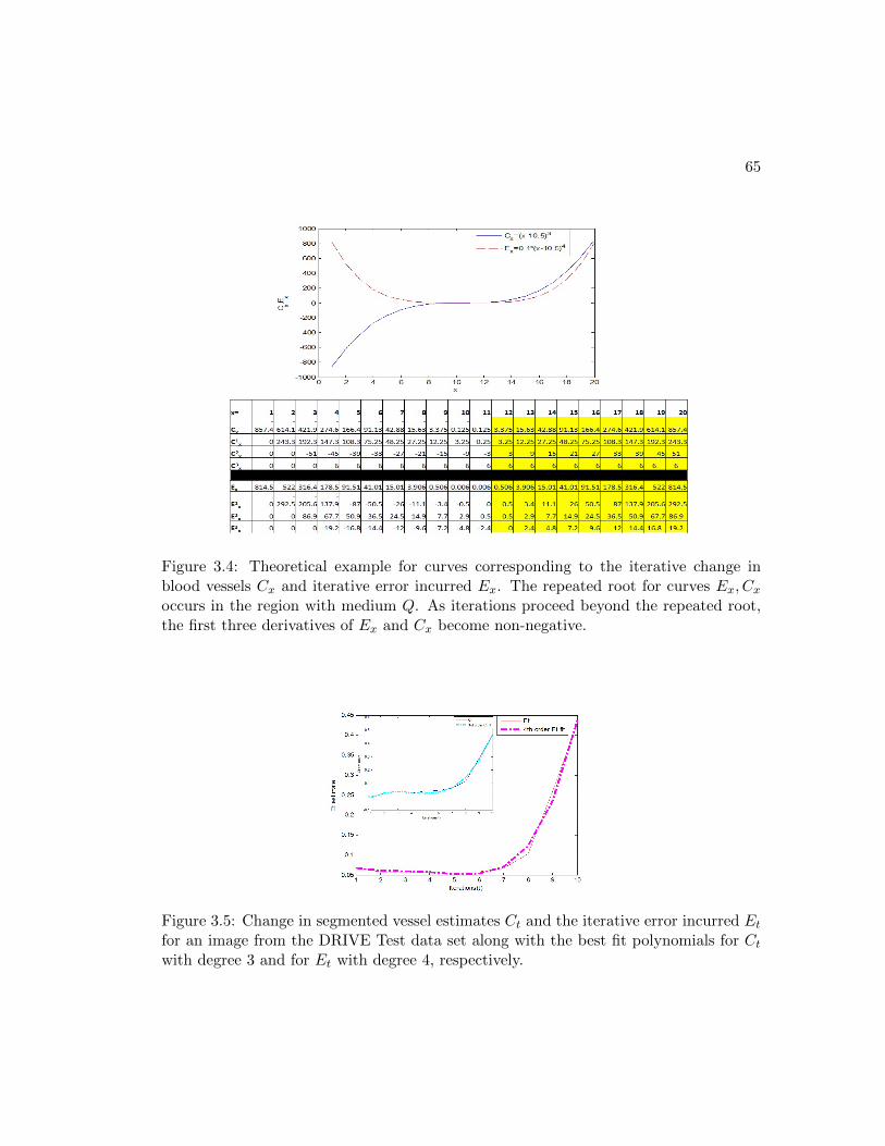
65

Figure 3.4: Theoretical example for curves corresponding to the iterative change inblood vessels Cx and iterative error incurred Ex. The repeated root for curves Ex, Cxoccurs in the region with medium Q. As iterations proceed beyond the repeated root,the first three derivatives of Ex and Cx become non-negative.

Figure 3.5: Change in segmented vessel estimates Ct and the iterative error incurred Etfor an image from the DRIVE Test data set along with the best fit polynomials for Ctwith degree 3 and for Et with degree 4, respectively.

66

(a)

(b)

Figure 3.6: The vessel estimate curves Ct and Et for a particular image from (a) DRIVETest, and (b) STARE, respectively. The stopping iterations are (a) tf = 5, (b) tf =4. In (a) the three consecutive derivatives for Et and Ct become non-negative at thesame iteration step. In (b), the iteration for three consecutive non-negative derivativescorresponding to Ct and Et are different.

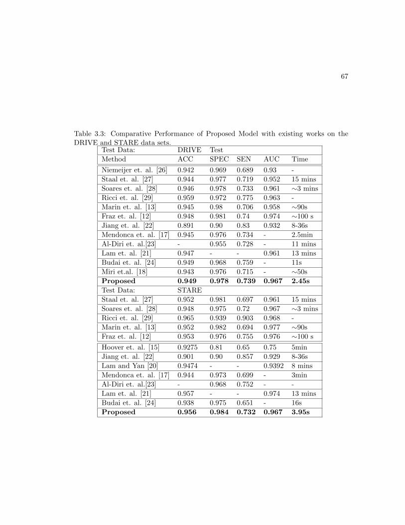
67

Table 3.3: Comparative Performance of Proposed Model with existing works on theDRIVE and STARE data sets.

Test Data: DRIVE Test

Method ACC SPEC SEN AUC Time

Niemeijer et. al. [26] 0.942 0.969 0.689 0.93 -

Staal et. al. [27] 0.944 0.977 0.719 0.952 15 mins

Soares et. al. [28] 0.946 0.978 0.733 0.961 ∼3 mins

Ricci et. al. [29] 0.959 0.972 0.775 0.963 -

Marin et. al. [13] 0.945 0.98 0.706 0.958 ∼90s

Fraz et. al. [12] 0.948 0.981 0.74 0.974 ∼100 s

Jiang et. al. [22] 0.891 0.90 0.83 0.932 8-36s

Mendonca et. al. [17] 0.945 0.976 0.734 - 2.5min

Al-Diri et. al.[23] - 0.955 0.728 - 11 mins

Lam et. al. [21] 0.947 - - 0.961 13 mins

Budai et. al. [24] 0.949 0.968 0.759 - 11s

Miri et.al. [18] 0.943 0.976 0.715 - ∼50s

Proposed 0.949 0.978 0.739 0.967 2.45s

Test Data: STARE

Staal et. al. [27] 0.952 0.981 0.697 0.961 15 mins

Soares et. al. [28] 0.948 0.975 0.72 0.967 ∼3 mins

Ricci et. al. [29] 0.965 0.939 0.903 0.968 -

Marin et. al. [13] 0.952 0.982 0.694 0.977 ∼90s

Fraz et. al. [12] 0.953 0.976 0.755 0.976 ∼100 s

Hoover et. al. [15] 0.9275 0.81 0.65 0.75 5min

Jiang et. al. [22] 0.901 0.90 0.857 0.929 8-36s

Lam and Yan [20] 0.9474 - - 0.9392 8 mins

Mendonca et. al. [17] 0.944 0.973 0.699 - 3min

Al-Diri et. al.[23] - 0.968 0.752 - -

Lam et. al. [21] 0.957 - - 0.974 13 mins

Budai et. al. [24] 0.938 0.975 0.651 - 16s

Proposed 0.956 0.984 0.732 0.967 3.95s

68

(a)

(b)

Figure 3.7: (a) ROC curves for blood vessel segmentation on DRIVE test, STARE andCHASE DB1 data sets. (b) Variation in mean segmentation accuracy by varying thethresholds. Highest ACC is achieved for the DRIVE Test, STARE and CHASE DB1data sets with k = [1.4, 1.6, 1.6], respectively.

69

Figure 3.8: Vessel segmentation on abnormal images. First row depicts vessel segmen-tation on an image with red lesions while the second row depicts segmentation on animage with bright lesions. (a) Image. (b) Manually marked vessels. (c) Segmentationby Soares et. al. (d) Segmentation by Marin et. al. (e) Segmentation by proposedmethod.

Table 3.4: Segmentation Performance on the STARE Abnormal data set.Method ACC AUC Time

Hoover et. al. [15] 0.9211 0.7590 5 mins

Jiang et. al. [22] 0.9352 0.9343 8-36 s

Mendonca et. al. [17] 0.9426 - 3 mins

Soares et. al. [28] 0.9425 0.9571 3 mins

Vermeer et. al. [19] 0.9287 0.9187 -

Marin et. al. [13] 0.9510 - 90 s

Lam and Yan [20] 0.9474 0.9392 8 mins

Lam et. al. [21] 0.9556 0.9707 13 mins

Proposed 0.9535 0.9638 3.87 s

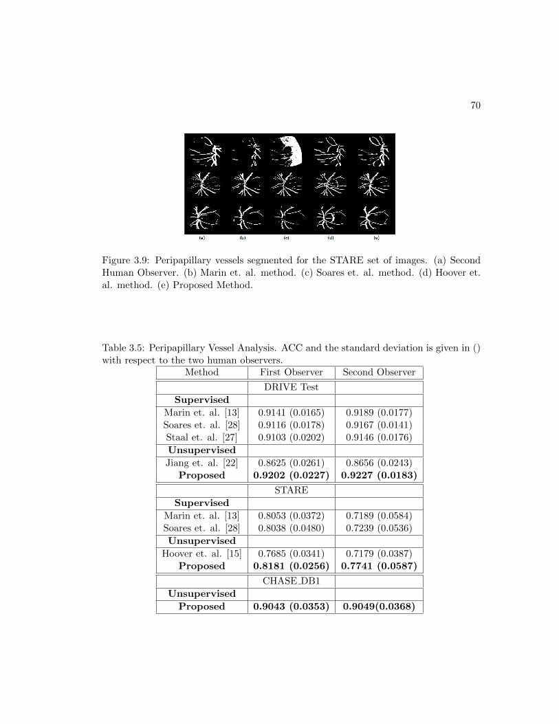
70

Figure 3.9: Peripapillary vessels segmented for the STARE set of images. (a) SecondHuman Observer. (b) Marin et. al. method. (c) Soares et. al. method. (d) Hoover et.al. method. (e) Proposed Method.

Table 3.5: Peripapillary Vessel Analysis. ACC and the standard deviation is given in ()with respect to the two human observers.

Method First Observer Second Observer

DRIVE Test

Supervised

Marin et. al. [13] 0.9141 (0.0165) 0.9189 (0.0177)Soares et. al. [28] 0.9116 (0.0178) 0.9167 (0.0141)Staal et. al. [27] 0.9103 (0.0202) 0.9146 (0.0176)

Unsupervised

Jiang et. al. [22] 0.8625 (0.0261) 0.8656 (0.0243)Proposed 0.9202 (0.0227) 0.9227 (0.0183)

STARE

Supervised

Marin et. al. [13] 0.8053 (0.0372) 0.7189 (0.0584)Soares et. al. [28] 0.8038 (0.0480) 0.7239 (0.0536)

Unsupervised

Hoover et. al. [15] 0.7685 (0.0341) 0.7179 (0.0387)Proposed 0.8181 (0.0256) 0.7741 (0.0587)

CHASE DB1

Unsupervised

Proposed 0.9043 (0.0353) 0.9049(0.0368)

Chapter 4

Automated Optic Disc

Segmentation

4.1 Introduction

Automated detection of optic disc (OD) is important for early detection of glaucoma

[39]. Disc size, neuro-retinal rim and cup area features are used to detect a glaucomatous

retina [40]. OD and the position of vessel origin (VO) are the main anatomical features in

retinal fundus images. The VO position is an important reference point for detecting the

macula, and thereby grading macular pathologies such as diabetic maculopathy, macular

edema and macular ischemia [41]. Also, automated OD detection plays an important

role in developing automated “diagnosis expert systems” for diabetic retinopathy (DR),

as its segmentation is a key component to correctly identify other bright features in the

images such as the bright lesions (hard exudates or cotton-wool spots) [42] [3]. Besides

the position of the OD, the VO seed point is another important feature of a fundus

image that is needed for vessel tracking methods to detect vessel features like vessel

tortuosity and vessel branching patterns [42]. Also, automated segmentation of the OD

boundary and the VO position are essential for automated eye motion tracking during

laser surgeries [40].

The detection of the OD region is challenging due to the fact that the size, shape

and color of the OD vary from one person to another and with the field of view (FOV)

of the fundus images. Estimates regarding the size of the OD vary from one-seventh

71

72

of an entire image, or from one-tenth to one-fifth of the image [43]. Along with the

disparity in the size and shape of the OD in images, another challenge arises from

fundus images that depict a relatively dark OD due to illumination issues of the non-

mydriatic camera. Additionally, in images with multiple abnormalities, such as images

with myelinated nerve fiber, the detection of OD becomes significantly more challenging.

Also some prior works have failed to detect the OD in images with exudates similar in

shape and size as the OD [44]. Other concerns adding to the challenge of segmenting

the region of the OD include instances when peripapillary atrophy is present and the

shape of the OD is further distorted.

In this chapter, we detect the OD at the intersection of the largest red region and

one of the brightest regions in the fundus image such that the OD regions satisfy cer-

tain compactness constraints. The method of OD neighborhood region detection by

minimizing the intensity sum and maximizing the bright region solidity, i.e., Minimum

Intensity Maximum Solidity MinIMaS, has been presented in our earlier work [10]. In

this chapter, we modify this method to maximize the vessel-sum and solidity of OD

regions and propose a new algorithm referred as Maximum Vessel-Sum and Solidity

(MaxVeSS) to detect the OD candidate region. Also, in this chapter we extend our

analysis to segment the exact OD boundary and VO pixel location instead of just es-

timating the OD neighborhood region. This work will aid cup-to-disc ratio assessment

for glaucoma detection and screening algorithms.

In this chapter, we propose an OD detection algorithm that segments the OD region

with 100% success on 1487 retinal fundus images from 5 different public data sets with

FOV in the range [30o to 50o] and computes the vessel origin with less than 10 pixels

error in less than 5 seconds per image. The proposed algorithm relies on the structure of

the bright regions in fundus images and their relative positions in the neighborhood of

the biggest red region (the retinal blood vessels) to detect the OD region. The proposed

algorithm consistently estimates the OD region such that 94.37% of the total images

under evaluation have higher than 70% overlap between the manually segmented OD and

the automatically segmented OD. This chapter makes three key contributions. First,

selection of a circular structuring element, as opposed to linear during morphological

transformation leads to significantly high accuracy in detecting the OD boundary and

less error in detecting the VO. Second, the proposed MaxVeSS algorithm detects the

73

OD neighborhood with high accuracy. Third, the OD detection and VO location are

computed by the same algorithm; these were treated as two separate problems in the

past. The significance of this chapter is two-fold. First, the proposed OD boundary

and VO detection algorithms presented in this chapter are the fastest reported so far.

Second, the proposed OD segmentation algorithm is robust to variations in retinal

images caused due to illumination artifacts or retinal abnormalities such as myelination

or peripapillary atrophy.

The organization of this chapter is as follows. In Section 4.2, the existing OD

detection and segmentation methods are reviewed. In Section 4.3, the proposed OD

segmentation algorithm is presented. In Section 4.4 the experimental results of auto-

mated OD segmentation are presented. Conclusions and discussion are presented in

Section 4.5.

4.2 Overview of Prior Work

Related work regarding OD detection using fundus images can be broadly categorized

into two groups: 1) those based on the shape, color and structure of OD, and 2) those

based on the properties of the retinal vasculature. The first category includes well-

known methods that rely on the appearance and size of the OD [45], such as methods

utilizing the highest average variation among adjacent pixels in a specific window size

similar to that of the OD [43].

Other methods belonging to the first category include model-based approaches such

as the template-matching method that made use of averaging of color-normalized im-

ages to yield a gray template, followed by computation of the normalized correlation

coefficient to find the best match between the template and test images in [46]. Addi-

tionally, the Hausdorff-based template matching method used pyramidal decomposition,

which aided the detection of large candidate objects in the image, followed by the com-

putation of a confidence level for each OD candidate region based on the ratio of the

mean intensity inside and in the immediate neighborhood of the candidate in [47]. Yet

another method identified the OD location using template matching and directional

matched filter in [48]. Further, the OD segmentation was performed using a fast hy-

brid level-set algorithm that combined the OD region information and edge gradient to

74

estimate the evolution of the OD curve. The first category also relates to algorithms

that apply various transformations to images, such as the Haar-based discrete wavelet

transform on the green plane of the image to create a resolution pyramid, where the

brightest pixel at the fifth level of the pyramid is selected as the OD in [45]. Also,

the Circular Hough transform has been employed to detect a large circular OD in [39]

after the edges were detected in an image by applying the Sobel operator followed by

thresholding. The method in [42] first located a pixel belonging to the OD region, and

then applied boundary segmentation by morphology, edge detection and circular Hough

transforms.

The second category of methods examine the retinal vasculature for locating the

OD, since the OD is the point of entrance of the optic nerve and blood vessels which

branch out into finer vessels through the retina. One such method in [44] used a fuzzy

convergence algorithm that analyzed six binary vessel segmentations obtained from the

green plane of the image to construct a cumulative voting image or a convergence im-

age which was smoothened and thresholded to determine the best convergence point.

Another method in [45] applied a search on the branching network patterns formed by

the blood vessels to converge to the region where most paths ended, followed by the

application of Hough transform on all such regions to finally locate the OD. Another

method in [49] applied an OD template using the Laplacian of Gaussians to extract the

vertical edges of the main blood vessels in the OD, which was correlated to the inten-

sity of the test images using the Pearson-R correlation. The method in [50] localized

the OD by tracking the blood vessels using Gabor filters to detect the peaks in nodes

via phase portrait analysis and located the OD at the focal point of the vessels using

Hough transform. A graph-based approach in [51] applied graph-cut techniques with

compensation terms associated with the blood vessels based on the relationship between

neighbor pixels and likelihood of the pixels to belong to foreground or the background

based on prior information. The method in [52] applied watershed transform for de-

tecting the OD location and disc boundary using the information regarding the major

vessel arcade. Besides, maximization of vessel pattern-based entropy is used to detect

the location of the OD in [53].

Some algorithms, however, have combined the two categories such as the method

that locates the OD based on the structure of the OD, the convergence of blood vessels

75

at the OD and the variation in the size of the blood vessels entering the OD in [54].

Another method used the feature based k-nearest neighbor (kNN) classifier for training

and extracting the OD in [55]. Also, another model located the OD by fitting a 16-

point distribution model as an anatomical template to images by optimizing the cost

function that was represented by the probabilistic vessel orientation, the width atlases

and kNN based distance regression at pixel level in [56]. The method in [41] proposed

an ensemble of pyramidal decomposition, edge detection, entropy-filter based detection,

Hough transform and feature vector based algorithms for detecting the OD. Another

method in [57] used the principal component image plane followed by removal of vessel

regions, image inpainting, stochastic watershed transform and regional discrimination

for the OD boundary detection.

Most existing works focusing on OD segmentation deal with OD localization or OD

boundary segmentation, but not both [52]. In this chapter we propose a method that

combines the two categories of OD segmentation such that the brightness, compactness,

elliptical extent and vicinity of the blood vessels are properties to identify the OD

boundary and the VO location. The proposed algorithm is computationally simple and

it has consistent OD segmentation performances on both normal and abnormal retinal

images.

4.3 Materials and Method

In this chapter, we propose a novel rule-based OD boundary segmentation and VO

detection algorithm generalizable across data sets comprising of retinal images with

varying fields of view (FOV), varying contrast and illumination intensities and varying

retinal abnormalities. This algorithm is implemented on a Laptop (2.53 GHz Intel Core

i3 and 2Gb RAM) using MATLAB. Although OD is generally the brightest element

in retinal images, the entire OD region is not equally brightly illuminated. The thick

blood vessels at the OD separate the OD region into several smaller brightly illuminated

regions. For accurate boundary detection of the complete OD, it is imperative to detect

all such bright OD regions. To facilitate this, we propose a two-step approach, where

in the first step, the brightest OD candidate region is detected and its neighborhood is

selected as the OD neighborhood region. In the second step, additional bright regions are

76

detected within the OD neighborhood. A convex hull is then created around all bright

regions retained within the OD neighborhood region and a best fit ellipse around this

convex hull is the segmented OD boundary. Finally, the position of VO is determined

at the centroid of the blood vessels that lie within the segmented OD boundary.

The first step for OD segmentation regarding the identification of the brightest

OD candidate region and the OD neighborhood is the most critical operation since the

structure and pixel intensities of the OD region vary across fundus images. For instance,

in some abnormal fundus images from patients with non-proliferative DR, bright lesions

such as hard exudates and cotton-wool spots have similar structural compactness and

brightness as the OD. Also, abnormal fundus images with myelinated nerve fiber may

contain such structurally identical and bright regions as the OD. To facilitate accurate

OD identification in normal and abnormal fundus images, we implement a Maximum

Vessel-Sum and Solidity (MaxVeSS) algorithm that detects the OD neighborhood as

the region where the reddest and brightest regions of the fundus image intersect under

some vessel intensity and region compactness constraints.

4.3.1 Data

For OD segmentation performance analysis, retinal images are manually annotated for

the OD boundary (D) and the pixel corresponding to the VO (O) using the GIMP soft-

ware [58]. The proposed OD segmentation algorithm is tested on fundus images from the

following publicly available data sets. All the images from the DRIVE, DIARETDB0,

DIARETDB1 and CHASE DB1 are manually annotated for the OD boundary and VO

pixel location.

• DRIVE [59] data set contains 40 images with 45o FOV and size of [584x565] or

[730x490] pixels.

• DIARETDB1 [60] data set contains 89 images with 50o FOV and size of [1500x1152]

pixels.

• DIARETDB0 [61] data set contains 130 images with 50o FOV and size of [1500x1152]

pixels.

• CHASE DB1 [30] data set contains 28 images with 30o FOV and of size [960x999]

77

pixels. These images correspond to two images per patient (one image per eye)

for 14 children [12].

• MESSIDOR [62] data set, contains 1200 images with 45o FOV in 3 sets of 400

images each from 3 ophthalmic departments named Laribiosiere, CHU de Etienne

and LATIM-CHU de BREST, respectively. Each image is of size [1440x960],

[2240x1488], or [2304x1536] pixels respectively. The manual annotations for OD

boundary of each image is obtained from [57]. The VO pixel is manually segmented

for 500 images that are sub-categorized as Base 24 (data from CHU de St Etienne),

Base 31, Base 32, Base 33 and Base 34 (data from LATIM-CHU de BREST) by

the authors.

4.3.2 Proposed Method

OD in a retinal fundus image is generally the brightest and the most compact structure

lying in the vicinity of blood vessels that are the thickest at the point of vessel origin

and become narrow as they branch away from the OD. The proposed algorithm incor-

porates this retinal structure property to extract the major blood vessels and the bright

regions in a fundus image. Next, the OD is detected as the bright region with highest

compactness and the most number of blood vessel pixels in its vicinity [52] [53]. As a

pre-processing step, the green plane of each color fundus image is resized to [500x500]

and the pixel intensities are scaled in the range [0,1], followed by contrast enhancement,

resulting in image I. Next, I is morphologically eroded using a structuring element, fol-

lowed by image reconstruction. This reconstruction operation enhances the compactness

of brightly illuminated regions that include bright lesions, OD and contrast variations

around the blood vessels. The reconstructed image is then subtracted from I, scaled

in [0,1], and subjected to contrast enhancement to yield a morphologically transformed

image Ir.

Selection of a structuring element for the morphological transformation of image

I to Ir is key to the detection of OD boundary. While image erosion with a small

structuring element can disintegrate the OD into several small bright regions with low

compactness, a large structuring element can enlarge the OD boundary, thereby leading

to incorrect OD segmentation. The impact of linear and circular structuring elements

78

on an image from the DIARETDB0 data set is shown in Fig. 4.1. From Fig. 4.1 we

observe that circular structuring elements are most suitable for detecting the bright OD

regions. This is a key result of this chapter, as some prior morphological constructions

were based on linear structuring elements. The impact of this selection on accuracy of

OD detection and VO location is significant. Empirically, we observed that for resized

fundus images to [500x500] pixels, the average minor axis lengths of the actual OD

region for images from the DRIVE, DIARETDB0, DIARETDB1, CHASE DB1 and

MESSIDOR data sets are 73, 70, 60, 90 and 45 pixels, respectively. Since the OD is

divided into four major quadrants by the thick blood vessels, a circle as structuring

element with radius one quarter of the actual OD diameter is capable of extracting

one quadrant of the OD. Thus, for the image in Fig. 4.1, the minor axis length is 70

pixels, and a circular structuring element with radius 17 pixels extracts all the major

bright regions corresponding to the OD with the least error in OD boundary estimation.

Further, for the images from DRIVE, DIARETDB0, DIARETDB1, CHASE DB1 and

MESSIDOR data sets, a circular structuring element with radius 18, 17, 15, 22, 11,

respectively, are used for the morphological reconstruction.

Figure 4.1: Bright region extraction using different structuring elements for morpho-logical transformation. Top row represents morphologically transformed image Ir usinga horizontal linear structuring element of a certain length (Line, [pixel length]), or acircular structuring element with a certain radius (Circle, [pixel radius]). Second rowrepresents the image containing the bright regions obtained by thresholding the respec-tive image Ir. For this image from DIARETDB0 data set, a circular structuring elementwith radius 17 results in the best segmented OD.

The process of locating the OD neighborhood region, detecting the OD boundary

79

(D) and the VO location (O) is described below. The notations and their definitions

used in this OD detection algorithm are defined in Table 4.1.

OD Neighborhood Detection: The MaxVeSS Algorithm

To locate the vicinity of the OD region at the intersection of the largest red region and

the bright regions in image I as in [10], the major blood vessels and bright regions are

first detected. To extract the major blood vessel regions from I, a smoothened low-

pass filtered image LPF (I) is subtracted from I to obtain a high-pass filtered image.

Here, the low-pass filter is a median filter with window size [20x20] as used in [10]

[31]. This high-pass filtered image is then thresholded to extract pixels less than 0, and

the absolute pixel strengths of the thresholded image are contrast adjusted to extract

the major vessels Iv as shown in (4.1). An image with bright regions (Ib) is extracted

by adding the pixel intensities in Ir to the histogram equalized version of I, followed

by scaling the resultant image in [0,1] and thresholding at pixel intensity value 0.9 in

(4.2). Next, an Overlap function is defined with a neighborhood parameter ν = 30,

such that if pixels in Iv are located in the neighborhood of pixels in Ib, bright candidate

regions (R) are detected in Ib [10] using (4.3). Among all these bright candidate regions,

the regions that are highly elliptical (denoted by a high ratio of major and minor axis

lengths Φ(Re)Ψ(Re) > χ0, χ0 = 2.5) and less compact regions with ‘holes’ (denoted by the

ratio between the region area, (A(Re)), and filled area, (F (Re)),A(Re)F (Re) < η0, η0 = 0.95)

are discarded as shown in (4.4). ρ is calculated as the maximum major axis length

among all the bright candidate regions in (4.5).

Iv = [I − LPF (I)] < 0 (4.1)

Ib = [scale(Ir + histeq(I))]→ [0, 1] > 0.9 (4.2)

Re = Overlap(Iv, Ib, ν), e ∈ 1, 2, ...r (4.3)

Such that,∀e, Φ(Re)

Ψ(Re)≤ χ0,

A(Re)

F (Re)≥ η0. (4.4)

ρ = maxeΦ(Re). (4.5)

From all the bright candidate regions (R), the brightest candidate region for the OD

80

is selected based on two parameters: vessel-sum and solidity using (4.6). For computing

the vessel-sum, at each bright candidate region (Re), a circular mask is generated whose

center is at the centroid of Re with radius ρ. Next, the sum of pixel intensities of all

the vessel pixels in Iv lying within each such circular mask is computed as vessel-sum

by a function V essel-Sum(Re). Solidity of a bright candidate region is a measure of

the compactness of shape, and it is computed as the ratio of the area to the area within

a convex hull bordering the region (Solidity(Re) = A(Re)A(H(Re))) [10]. Now, the brightest

OD region must be the bright candidate region with Maximum Vessel-Sum and Solidity

(MaxVeSS. If the region with maximum vessel-sum is not same as the region with

maximum solidity (e1 6= e2), then the region with maximum vessel-sum is discarded

(R = R\Re1), and (4.6) is re-evaluated for the remaining regions till convergence is

achieved in (4.6).

Λ(R) = [e1, e2 : e1 = arg maxeV essel-Sum(Re), (4.6)

e2 = arg maxeSolidity(Re)].

ROD(Λ(R)) =

Re1 = Re2 : e1 = e2

ROD(Λ(R = R\Re1)) : e1 6= e2.(4.7)

Once the OD candidate region is detected as ROD, the centroid of this region is

detected as Θ(ROD), and the OD neighborhood region is detected as a circular region

centered at Θ(ROD) with radius ρ. This OD neighborhood is denoted by a sub-image

mask SROD .

The MaxVeSS algorithm detects the OD candidate region, the OD neighborhood

and also the major blood vessels as shown in Fig. 4.2. The exact OD boundary and VO

is then estimated using these segmented retinal components. It is noteworthy that for

some existing DR screening tools such as the one in [3], exact OD boundary detection is

not required since detection and masking out of the OD neighborhood removes instances

of false positives for bright lesion detection. Hence, the MaxVeSS algorithm can be a

useful module for such screening tools, especially for images with varying FOVs.

81

OD Boundary Detection

Once the OD neighborhood and the brightest OD candidate region are detected, the

next task is to detect the exact OD boundary. The morphologically reconstructed image

Ir is masked with the OD neighborhood mask (SROD) and thresholded, using threshold

parameter ω, to obtain an image containing bright regions. ω is computed using Otsu’s

threshold method from the superimposed image [Ir SROD ]. The bright regions are

then further subjected to region-based thresholding, where the bright regions that are

highly elliptical, or that have holes in them, or that have a significantly small area, are

discarded. The remaining bright regions are contained in image T , as defined in (4.8).

T =Ir SROD

> ω, : T = [Rk, k = 1, ...nk], (4.8)

such that,∀k, Φ(Rk)

Ψ(Rk)≤ χ, A(Rk)

F (Rk)≥ η,A(Rk) ≥ 30.

From all the retained bright regions in image T , the location of the OD candidate

region is detected as the region containing the pixel Θ(ROD) (i.e., Θ(ROD) ∈ ROD ⊆ T ).

Next, the bright regions in T that lie within one disc-diameter from ROD are detected

as the probable OD regions (P ). Thus, the bright regions in T whose centroids are

located within δ pixels from Θ(ROD) are included in image P in (4.9). A convex hull

(H) is then constructed around all the regions in P (4.10). Next, the centroid (Θ(H)),

the major axis length (Φ(H)) and minor axis length (Ψ(H)) of the convex hull H are

computed and an ellipse is fitted corresponding to these measurements. This best fit

ellipse is resized to the original image dimensions this is the segmented OD boundary

(D) in (4.11).

∀ T = [Rk|k = (1, ...nk])], ROD, identify P ⊆ T, (4.9)

P = [ROD ∪Rl : ||Θ(Rl)−Θ(ROD)||2 ≤ δ], l ≤ nk.

H ← Convex Hull (P). (4.10)

D ← Ellipse with [Φ(H), Ψ(H), Θ(H)]. (4.11)

82

The threshold parameters for OD boundary detection are empirically determined.

To determine the thresholds for images with 45 − 55o FOV, 5 images from the DI-

ARETDB0 data set were selected such that each image had significant bright lesions,

poor illumination or laser scar marks. On analyzing the compactness measures for the

OD regions and the scar or bright lesion regions on these 5 images, the threshold values

[χ, η, δ] were estimated for all the images from DRIVE, DIARETDB1, DIARETDB0,

and MESSIDOR data set as [4.4, 0.97, 54]. For the CHASE DB1 images with 30o FOV,

these threshold values were empirically determined using the first two images from the

left and right eye of the first patient as [3.4, 0.95, 60], respectively. The steps for detect-

ing bright regions within the OD neighborhood mask around the OD candidate region

and segmentation of the OD boundary are illustrated in Fig. 4.3.

Vessel Origin detection

Once the OD boundary is segmented, the next task is to detect the position from which

the optic nerve originates, or the pixel location of the VO. For this, a binary image mask

corresponding to the segmented OD boundary (SROD) is superimposed on the major

blood vessel image (Iv). The VO pixel (O) is located at the centroid of the vessels in

the resulting superimposed image. The steps to VO location detection are illustrated

in Fig. 4.4.

4.4 Results

4.4.1 Metrics

The robustness of the proposed method for OD boundary segmentation and VO pixel

detection is analyzed based on distribution of certain performance metrics. These per-

formance metrics are described in terms of the area of overlap between the manually

segmented actual OD (D) and the automated segmented OD (D), and the distance in

pixels between the segmented and manual ODs and VOs as shown in Fig. 4.5. For each

test image, the area of the manually marked OD also detected by the automated algo-

rithm (TP, true positive), area of the falsely detected OD by the automated algorithm

(FP, false positive), area of the actual OD missed by the automated segmentation (FN,

83

false negative), and area within the retinal region that is not the OD (TN, true negative)

are computed. The performance metrics to analyze the robustness of the proposed OD

segmentation algorithm are described as follows.

• S (Overlap Score) - It denotes the fraction of overlapping area between the ac-

tual and segmented OD, i.e., S =AD∩DAD∪D . Higher S denotes better automated

segmentation.

• M (Mean absolute OD distance) - It denotes the mean shortest distance in pix-

els between the circumference of the segmented and actual OD. To compute M ,

sample points are detected on the circumference of the segmented and actual disc

every 3o ranging from [0 to 360o]. Let the sampled points on the actual OD

be [X1, ....XnD ], while the points on the segmented OD be [Y1, ....YnD], where

nD = nD = 120. The shortest distance of each sampled point on the actual disc

from the sampled points on the segmented disc is computed using (12). Finally,

the mean of these distances is computed using (13). Smaller M denotes better

segmentation.

• SEN (Sensitivity) - It denotes the fraction of the actual OD area detected by the

automated algorithm. Higher SEN denotes better segmentation.

• FPR (False Positive Rate) - It denotes the fraction of falsely detected OD area.

Lower FPR denotes better segmentation.

• Acc (Accuracy) - It denotes the fraction of correctly identified pixels to the total

number of pixels in the retinal region, i.e., Acc = TP+TNTP+TN+FP+FN . Higher Acc

denotes better segmentation.

• ∆ (VO error) - It denotes the Euclidean distance in pixels between the manually

marked VO (O) and the detected VO (O). Smaller ∆ denotes better segmentation.

• Time- It denotes the average OD boundary segmentation and VO detection time

per image for the particular data set measured in seconds. The average processing

time is inversely proportional to the computational complexity of an automated

segmentation algorithm.

84

• Success (%) - It represents the percentage of images in a particular data set where

the OD is successfully identified. Successful OD identification occurs when the au-

tomatically detected VO (O) lies within the boundary of the manually segmented

disc (D).

∀ [Xi′ ∈ D : i′ = 1, ...nD], [Yj′ ∈ D : j′ = 1, ....nD], (4.12)

mD,D(i′) = minj′||Xi′ − Yj′ ||2,

mD,D(j′) = mini′||Yj′ −Xi′ ||2,

M =1

2

1

nD

nD∑i′

mD,D(i′) +1

nD

nD∑j′

mD,D(j′)

. (4.13)

The overlap score metric estimates the fractional area common to the actual and

segmented OD, while the mean absolute OD distance represents the closeness of fit

between the actual and segmented OD boundaries. The importance of analyzing both

these metrics together is illustrated using two examples in Fig. 4.6. In both these

examples, S metric is same, while the M metric varies. In such a case, the instance with

a lower M value represents a better segmented OD, since it enables better estimation

of blood vessel-based fiduciary points within the OD region.

The performance metrics for the OD segmentation algorithm are analyzed in terms of

the mean and standard deviation of the particular metrics across all images in each data

set under analysis, and the distribution of the overlap score, the mean absolute distance,

and the pixel error in the VO location. These performance metrics are analyzed with

respect to existing OD segmentation algorithms to assess the comparative robustness

of the proposed method.

4.4.2 Segmentation Performance

The OD mean and standard deviation of the OD segmentation performance metrics

using the proposed algorithm is shown in Table 4.2. While the OD boundary segmen-

tation analysis is performed on all 1200 images from the MESSIDOR data set, the VO

location is detected in 500 images that were manually annotated for this work. Hence,

85

the mean pixel error for VO location detection (∆) is evaluated on 500 images in the

MESSIDOR data set, and this change in the number of images under analysis is denoted

by the symbol + in Table 4.2.

We observe that the proposed algorithm has better averaged segmentation metrics

across all test images when compared to another recent algorithm in Morales et. al. [57].

Additionally, from Table 4.2, we observe that the proposed algorithm achieves mean ∆ =

7.36 in about 4.36 seconds per image. Also, the proposed OD segmentation algorithm

has a significantly low false positive region identification rate, thereby resulting in more

accurate OD boundaries and better fiduciary point estimation within the OD region.

Next, the comparative performance of the proposed OD boundary segmentation

algorithm with existing works is shown in Table 4.3. Here, we observe that for the

DRIVE data set, the proposed method has the best OD boundary segmentation metrics

so far. The proposed algorithm achieves significantly lower standard deviation forM and

100% OD segmentation success when compared to all other methods. This demonstrates

the robustness of the proposed algorithm to retinal variability due to pathology.

For the DIARETDB1 data set, we observe that the proposed method is out-performed

only by the stochastic watershed transform-based method in Morales et. al. [57].

However, the [FPF,Acc] achieved by the proposed method and the Morales et. al.

[57] method are [0.0017, 0.9963] and [0.0028, 0.9957], respectively. Thus, the proposed

method maintains a low false positive region detection rate in the test images from the

DIARETDB1 data set. For the MESSIDOR data set, only the method relying on the

Circular-Hough transform in Aquino et. al. [42] outperforms the proposed method in

terms of the overlap score S. This variation in S is mostly due to the difference in man-

ual markings and the variation introduced by down-sampling each image to [500x500]

followed by image resizing at the end of OD boundary detection. However, the average

OD boundary segmentation time taken by the method in Aquino et. al. [42] and the

proposed method are 5.69 seconds and less than 4.47 seconds, respectively. Hence, the

image resizing operation is beneficial from the computational complexity standpoint.

Next, in Table 4.4, we analyze the comparative performance of the proposed method

for detecting the VO pixel. Here, we observe that the proposed algorithm achieves

the lowest VO detection error in terms of ∆ in the least computational time, and a

‡ Mean and standard deviation computed for 500 manually marked images.

86

consistent OD segmentation success rate of 100% over all the test data sets. We point

out that the use of a circular structuring element, instead of linear, in the morphological

transformation step led to an improvement of 8% and 5% in the overlap score (S),

reduction of 2.25 and 1.25 pixels in mean distance (M), and error reduction of 1.22 and

1.9 pixels in VO location for DRIVE and DIARETDB1 databases, respectively.

Examples of the best and worst OD segmentation performance obtained using the

proposed algorithm on the images from all the 5 public data sets are shown in Fig.

4.7. We observe from the worst automated segmentation instances that the proposed

algorithm has significant OD segmentation accuracy in retinal images with improper

illumination and pathology. The images with least automated segmentation accuracy

from MESSIDOR data set have blurred OD boundary due to prominent peripapillary

atrophy. The proposed method is successful in detecting the OD neighborhood region

in these images, but the exact automated OD boundary detection for such images is

challenging. Further, in Fig. 4.8, we observe that the proposed algorithm is robust to

fundus images with retinal abnormalities around the OD region, such as images with

myelination and peripapillary atrophy with relatively low severity.

4.4.3 Distribution of Performance metrics

The overlap score between manually annotated disc and the segmented disc is regarded

as a significant indicator of OD segmentation accuracy [42] [52]. Analysis of the S metric

distribution on the test data sets is shown in Table 4.5. We observe that for all the test

data sets, the proposed method has the highest percentage of image with S ≥ 0.7. For

the DRIVE data set, the distribution of the S metric is significantly better than the

methods in Salazar et. al. [51]. For the MESSIDOR dataset, the method in Aquino

et. al. [42] has better performance for S > 0.75. However, the proposed algorithm

demonstrates consistent performance on this data set with 96% images having S ≥ 0.7.

Additionally, the fit between the segmented and actual OD boundary has been

extensively used to demonstrate the performance of OD segmentation algorithms in

[48] [41]. The MESSIDOR data set contains 400 images from three data subsets named:

CHU de St Etienne, LaTIM-CHU de BREST, and Lariboisiere and thus, it represents a

wide variety of images with varying severities of pathologies, the distribution of the M

metric has been analyzed on this data set in existing works [48] [42]. For comparative

87

analysis of the OD boundary segmentation performance, the distributions of the M

metric for the images from the MESSIDOR data set are shown in Table 4.6. Based

on the M metric, and assuming the average OD radius to be 70 pixels for the images

from the MESSIDOR data set [41], four categories of OD boundary segmentation can

be defined as: Excellent (M ≤ 3.5), Good (M ≤ 7), Fair (M ≤ 703 ), and Poor (M > 70

3 )

[48]. From Table 4.6, we observe that the proposed algorithm has more images in the

Excellent, Good and Fair segmentation category than the existing methods.

Finally, the distributions of the M metric and ∆ metric on all the test data sets are

shown in Fig. 4.9. Since low values of both these metrics indicate good OD segmentation

accuracy, hence the percentage of images in each data set that have [M ≤ mean(M)]

and [∆ ≤ mean(∆)] are shown in Table 4.7. Here, we observe that for all the data sets,

more than 53% of the images have small ∆ values, and more than 55% images have low

M metric. The average OD radius for all the images from the DRIVE, DIARETDB1,

DIARETDB0 and MESSIDOR data sets has been estimated as 60-70 pixels in [52],

[48], while for the CHASE DB1 data set, the average OD radius is measured to be 90

pixels. From Fig. 4.9, we observe that the proposed segmentation method achieves ∆

consistently less than 35 pixels for all test images, thereby ensuring 100% success of OD

segmentation.

4.5 Conclusions and Discussion

In this chapter, we have proposed a rule-based OD segmentation algorithm that is robust

to fundus images with varying FOV, illuminations and pathologies. Since the complete

OD region is not equally brightly illuminated, portions of the complete OD are detected

in two steps. In the first step, the brightest and most compact OD candidate region is

detected at the intersection of the bright regions and the retinal vasculature. Also, the

OD neighborhood is detected in this step. In the second step, additional bright OD re-

gions within the OD neighborhood are detected based on two compactness parameters,

which are, the ratio of area and convex area and ratio of the area to the filled area. A

convex hull is then estimated around all the bright candidate OD regions and a best fit

ellipse corresponding to the centroid, major and minor axis lengths of this convex hull

is estimated as the segmented OD boundary. The centroid of the major blood vessels

88

within detected OD boundary is the VO location. The proposed algorithm is the fastest

segmentation method reported so far and it results in consistent OD boundary segmen-

tation and VO location detection across normal and pathological retinal images. The

OD boundary segmentation performance of the proposed algorithm has lower standard

deviation in the error between manually segmented and automatically estimated OD

boundary when compared to recent works in [57]. The high computational speed can

be attributed to the down sampling all the fundus images to [500x500] followed by up

sampling to original image dimensions at the end of the OD boundary detection step.

Although this down and up sampling method introduces some errors in the segmented

OD boundary, these errors are significantly small when compared to the computational

speed thus achieved.

In this chapter the compactness of the bright OD regions is determined by two

metrics. The first metric is the ratio of the area and convex area for a bright region.

A high value for this metric denotes compact OD region boundaries when compared to

bright lesions such as hard exudates that contain irregular edges and have a low value

for this metric. The other compactness metric is the ratio of area to the filled area,

such that a bright OD region would have a high value for this metric, while regions with

‘holes’ in them would have a lower value. This metric further eliminates bright lesion

regions. These two compactness metrics are more effective for automated OD region

segmentation when compared to the metrics defined in prior works, such as the ratio of

squared perimeter to the area of a bright region in [52].

The most important feature of the proposed segmentation algorithm is that it is

a rule-based method and generalizable to images with FOV varying from [40o to 55o]

where the OD is always present in the fundus image. For images with [30o to 35o], the

OD may not be present in particular angles of the retinal shots. In such cases, if a

portion of the OD is visible in the image, an OD boundary is correctly estimated as

shown in the first example of Fig. 4.10. However, if the OD is entirely absent in the

fundus image, and then a false OD region may be detected by the proposed algorithm as

shown in the second and third examples in Fig. 4.10. In such situations, the thickness

of the major blood vessels within the segmented OD region can be analyzed to discard

these instances of false OD detection. It is known that the blood vessels are thickest at

the OD in any retinal image. Hence, as a post-processing step in images with [30o to

89

35o] FOV, the segmented OD region mask is superimposed on the blood vessel image

followed by image erosion using linear structural element of size 7-15 pixels at 0 degree

and 90 degree orientations. If OD exists in a particular image, then the thickness of the

small eroded regions should be greater than 10-15 pixels. Otherwise, the OD boundary

is discarded to eliminate falsely segmented OD regions. Future work will be directed

towards accurate blood vessel thickness estimation at the OD region for detecting neo-

vascularization at the optic disc and hypertensive retinopathy.

The other important feature of the proposed algorithm is that it robustly detects

the OD boundary and VO in retinal images with additional abnormalities around the

OD region. For instance in images with myelinated nerve fiber and peripapillary atro-

phy, existing methods [48] have resulted in poor segmentation performance while the

proposed algorithm has fair to good OD segmentation performance on such images. Fu-

ture work will be directed towards combining the proposed algorithm with automated

glaucoma detection algorithms that measure the variations in cup-to-disc ratio to detect

the disease severity.

90

Table 4.1: Definition of Notation.Notation Meaning

I Pre-processed green plane of the fundus image.

Ir Morphological reconstruction of the green plane image.

Iv Blood vessel image obtained by high-passfiltering and thresholding I.

Ib Bright region image obtained by thresholding Ir.

Overlap Function that retains regions in Ib that are closer(Iv, Ib, ν) to the regions in Iv than ν pixels.

Φ(Re) Major axis length of a region Rwith index number ‘e’.

Ψ(Re) Minor axis length of a region Rwith index number ‘e’.

A(Re) Area of a region R with index number ‘e’.

F (Re) Area after holes in region Rwith index number ‘e’ are filled.

ρ Maximum major axis length among allbright candidate regions.

Solidity(Re) Function computing the ratio of the area and convexarea for a particular region R with index number ‘e’.

V essel-Sum Function computing the sum of vessel pixels from(Re, ρ) image Iv within a circular masked region generated

at the centroid of region Re with radius ρ.

Θ(Re) Centroid pixel of a region Re.

ROD OD candidate region that has the highestsolidity and highest vessel sum in its neighborhood.

SROD OD neighborhood mask generated around region ROD.

T Thresholded image from Ir SROD .

P Image obtained by retaining the bright regions in T thatare less than ‘δ’ pixels away from the region ROD.

H Convex hull containing the all regions in the image.

D Best fit ellipse around H.

O Segmented VO pixel.

91

(a) (b) (c)

(d) (e) (f)

(g) (h)

Figure 4.2: Steps involved in extracting the brightest OD sub-region and the OD neigh-borhood. (a) Original image from DIARETDB0. (b) Morphologically reconstructedimage Ir. (c) Major vessels extracted as Iv. (d) Bright regions extracted in image Ib.(e) Intersecting bright candidate regions (R in blue) and the vessel regions (red). (f)Solidity of regions in R is computed. The region depicted by red arrow is discardedsince that region has ‘holes’ in it, i.e., A(Re)

F (Re) < η0. The region depicted by yellow arrow

has the maximum solidity. (g) Circular discs estimate vessel-sum within them for eachregion in R. The region with yellow boundary has the maximum vessel-sum. (h) ODneighborhood detected (SROD).

92

(a) (b) (c)

(d) (e) (f)

(g) (h)

Figure 4.3: The OD boundary segmentation steps for an image from DIARETDB0 dataset. (a) OD neighborhood mask (SROD). (b) Superimposed image Ir SROD . (c) Brightregions detected in image T after thresholding image (b). (d) The OD candidate region(ROD) is located among the bright regions in T . (e) Bright regions in T that are closeto the ROD are retained as image P . (f) Convex hull (H) constructed around all regionsin image (e). (g) Best fit ellipse to the convex hull. (h) The segmented OD boundary(D).

Table 4.2: Mean performance metrics and their standard deviation () of the ProposedMethod on the test data sets.‡

Data S M SEN FPR Acc ∆ Time

DRIVE 0.8165 (0.097) 4.87 (3.49) 0.8967 (0.077) 0.0021 (0.0023) 0.9959 (0.0043) 9.16 (4.21) 4.71 (3.21)

DIARETDB1 0.8060 (0.074) 4.15 (1.59) 0.8855 (0.057) 0.0017 (0.001) 0.9963 (0.001) 6.80 (3.56) 3.84 (1.69)

DIARETDB0 0.7774 (0.093) 4.91 (2.44) 0.8660 (0.068) 0.0021 (0.001) 0.9956 (0.002) 7.53 (4.76) 3.79 (0.87)

CHASE DB1 0.8077 (0.075) 5.19 (2.03) 0.8962 (0.047) 0.0032 (0.001) 0.9941 (0.002) 8.09 (4.34) 3.63 (0.35)

MESSIDOR 0.8331 (0.075) 3.39 (1.58) 0.9143 (0.072) 0.0015 (0.0008) 0.9979 (0.001) 7.31 (4.19)‡ 4.47 (2.00)‡

93

(a) (b) (c)

Figure 4.4: The VO pixel location steps. (a) Superimposed image SROD Iv. (b) Thecentroid pixel denoted by red arrow. (c) The VO pixel located.

Figure 4.5: The metrics used to evaluate the performance of automated OD segmenta-tion.

(a) (b)

Figure 4.6: Examples of automated OD segmentation performance. In both cases S = 13 .

M is estimated using 4 sample points on the actual and OD boundaries denoted by thesolid black dots. (a) has higher M than (b), hence (b) is a better segmentation.

94

Table 4.3: Comparative Performance of OD Boundary Segmentation with existingworks.

Method S M SEN Success (%)

DRIVE

Soparaphak et. al.[63] 0.179 (0.06) 20.94 (15.6) 0.80 98.61Walter et. al.[64] 0.300 (0.13) 12.39 (8.3) - 77.5

Seo et. al.[65] 0.316 (0.09) 11.19 (4.1) - 95Kande et. al.[66] 0.287 (0.08) 17.42 (8.1) - 95Stapor at. al.[67] 0.325 (0.15) 9.85 (6.0) - 87.5

Lapuscu et. al.[68] 0.403 (0.08) 8.05 (7.6) - 95Welfer et. al.[52] 0.415 (0.08) 5.74 - 100Zeng et. al.[69] 0.559 10.24 0.65 85

Boykov et. al.[70] 0.553 9.97 0.74 95Salazar et. al.[51] 0.707 6.68 0.84 97.5Morales et. al.[57] 0.716 (0.17) 5.85 (10.2) 0.854 100

Proposed 0.816 (0.09) 4.87 (3.5) 0.9 100

DIARETDB1

Soparaphak et. al.[63] 0.298 (0.09) 16.31 (5.3) 0.80 93.70Walter et. al.[64] 0.372 (0.11) 15.52 (5.3) - 92.13

Seo et. al.[65] 0.353 (0.07) 9.74 (4.6) - 80.89Kande et. al.[66] 0.332 (0.05) 8.35 (3.2) - 88.76Stapor at. al.[67] 0.341 (0.09) 6.02 (5.6) - 78.65

Lapuscu et. al.[68] 0.309 (0.13) 13.81 (9.1) - 86.51Welfer et. al.[52] 0.434 (0.11) 8.31 (4.1) - 97.7Zeng et. al.[69] 0.384 17.49 0.55 75.28

Boykov et. al.[70] 0.540 10.74 0.76 85.4Salazar et. al.[51] 0.757 6.38 0.86 96.7Morales et. al.[57] 0.817 (0.13) 2.88 (3.0) 0.922 100

Proposed 0.806 (0.07) 4.15 (1.6) 0.89 100

MESSIDOR

Yu et. al.[48] 0.83 7.7 - 98.3Aquino et. al.[42] 0.86 - - 100Morales et. al.[57] 0.823 (0.14) 4.07 (6.1) 0.93 100

Proposed 0.833 (0.07) 3.39 (1.6) 0.91 100

95

Table 4.4: Comparative Performance of VO detection with existing works.

Method ∆ Success (%)

DRIVE

Soparaphak et. al.[63] 16.98 98.61Yu et. al.[71] - 97.5

Lalonde et. al.[47] 13.21 97.22Ravishankar et. al.[72] 14.67 86.10

Qureshi et. al.[41] 15.95 100Niemeijer et. al.[73] 20.69 67.35

Rangayyan et. al.[50] 23.2 100Dehghani et. al.[74] 15.9 100

Proposed 9.16 100

DIARETDB1



Qureshi et. al.[41] 11.95 94.02Niemeijer et. al.[73] 20.41 77.04Youssif et. al.[75] 17 100

Proposed 6.80 100

DIARETDB0



Qureshi et. al.[41] 12.23 96.79Niemeijer et. al.[73] 18.55 78.20

Proposed 7.53 100

96

Figure 4.7: Best and worst OD segmentation performances achieved using the proposedalgorithm. The first two columns demonstrate the best OD segmentation cases. Thirdand fourth columns demonstrate the worst OD segmentation cases. The dotted blueoutline represents the manually annotated OD (D) while the solid black circle representsthe automatically segmented OD (D). The cyan (*) represents the manually marked VO(O), while the black (*) represents the automated VO detected (O). For all the worstcase performances, the automated VO lies within the manually marked OD boundary,thereby showing that the proposed OD segmentation algorithm has 100% ACC on allthe 5 public data sets.

97

Figure 4.8: Examples of automated OD segmentation on images, taken from the MES-SIDOR data set, with abnormalities around the OD regions. First column shows theoriginal image. Second column shows the reddest and bright region overlapping usingthe MaxVeSS algorithm. Third column shows the OD neighborhood mask superim-posed on the green plane image I. Fourth column shows the bright regions (T ) in blacksuperimposed on the image I. The brightest OD candidate region (ROD) is indicatedby the arrow. The fifth column shows the final best-fit ellipse detected (solid black line)and VO detected (black *) compared to the manually segmented OD boundary (dottedblue line) and manual VO (cyan *).

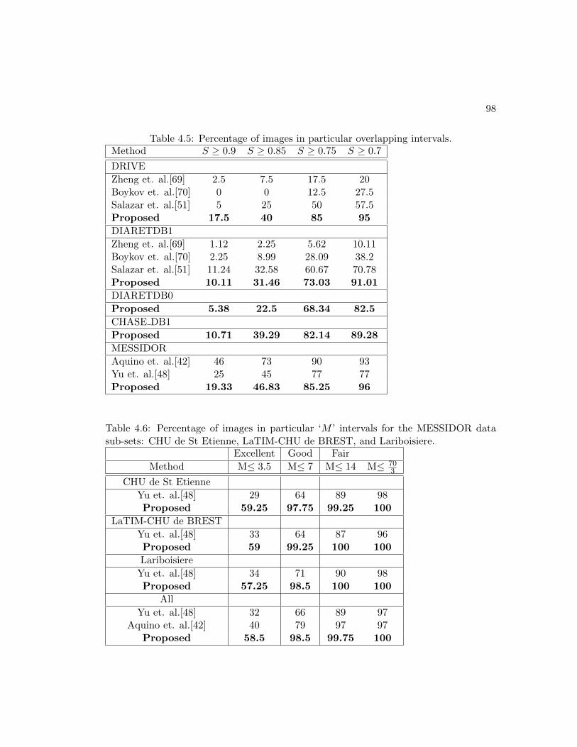
98

Table 4.5: Percentage of images in particular overlapping intervals.Method S ≥ 0.9 S ≥ 0.85 S ≥ 0.75 S ≥ 0.7

DRIVE

Zheng et. al.[69] 2.5 7.5 17.5 20Boykov et. al.[70] 0 0 12.5 27.5Salazar et. al.[51] 5 25 50 57.5Proposed 17.5 40 85 95

DIARETDB1

Zheng et. al.[69] 1.12 2.25 5.62 10.11Boykov et. al.[70] 2.25 8.99 28.09 38.2Salazar et. al.[51] 11.24 32.58 60.67 70.78Proposed 10.11 31.46 73.03 91.01

DIARETDB0

Proposed 5.38 22.5 68.34 82.5

CHASE DB1

Proposed 10.71 39.29 82.14 89.28

MESSIDOR

Aquino et. al.[42] 46 73 90 93Yu et. al.[48] 25 45 77 77Proposed 19.33 46.83 85.25 96

Table 4.6: Percentage of images in particular ‘M ’ intervals for the MESSIDOR datasub-sets: CHU de St Etienne, LaTIM-CHU de BREST, and Lariboisiere.

Excellent Good Fair

Method M≤ 3.5 M≤ 7 M≤ 14 M≤ 703

CHU de St Etienne

Yu et. al.[48] 29 64 89 98Proposed 59.25 97.75 99.25 100

LaTIM-CHU de BREST

Yu et. al.[48] 33 64 87 96Proposed 59 99.25 100 100

Lariboisiere

Yu et. al.[48] 34 71 90 98Proposed 57.25 98.5 100 100

All

Yu et. al.[48] 32 66 89 97Aquino et. al.[42] 40 79 97 97

Proposed 58.5 98.5 99.75 100

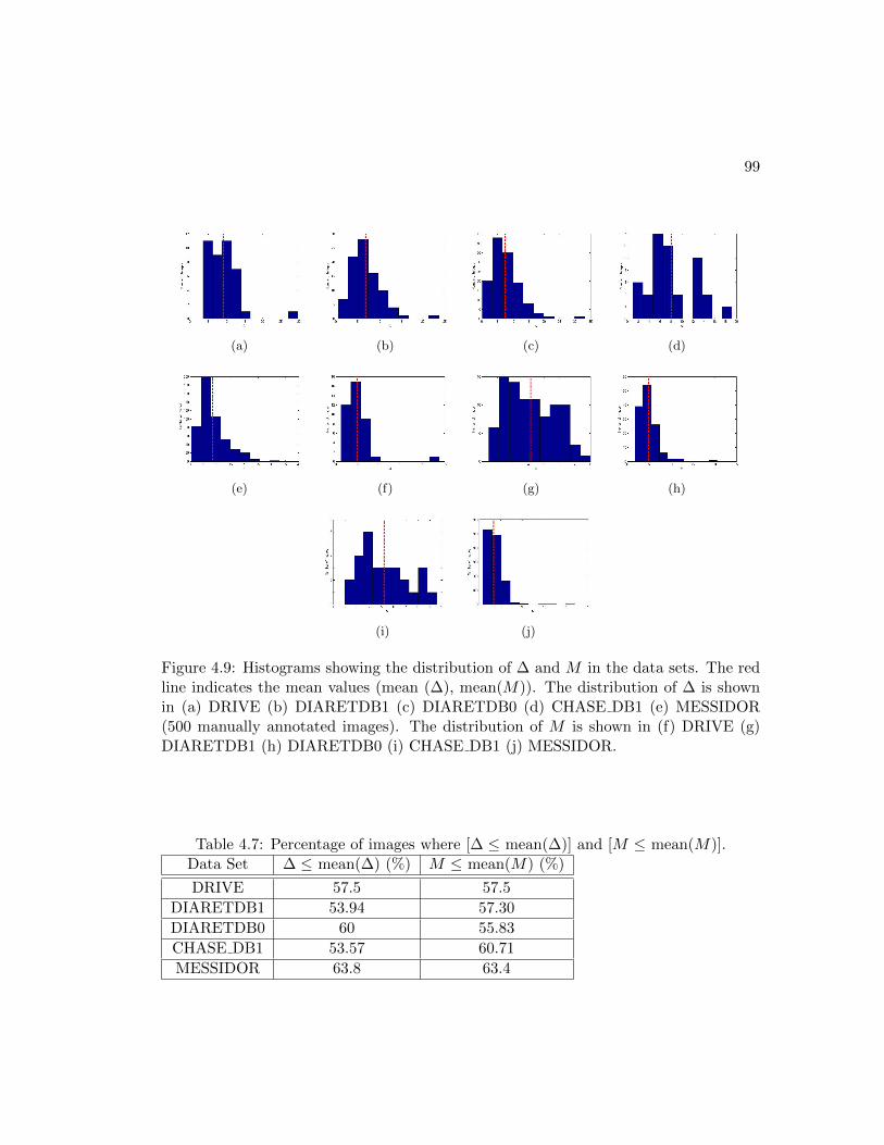
99

(a) (b) (c) (d)

(e) (f) (g) (h)

(i) (j)

Figure 4.9: Histograms showing the distribution of ∆ and M in the data sets. The redline indicates the mean values (mean (∆), mean(M)). The distribution of ∆ is shownin (a) DRIVE (b) DIARETDB1 (c) DIARETDB0 (d) CHASE DB1 (e) MESSIDOR(500 manually annotated images). The distribution of M is shown in (f) DRIVE (g)DIARETDB1 (h) DIARETDB0 (i) CHASE DB1 (j) MESSIDOR.

Table 4.7: Percentage of images where [∆ ≤ mean(∆)] and [M ≤ mean(M)].Data Set ∆ ≤ mean(∆) (%) M ≤ mean(M) (%)

DRIVE 57.5 57.5

DIARETDB1 53.94 57.30

DIARETDB0 60 55.83

CHASE DB1 53.57 60.71

MESSIDOR 63.8 63.4

100

Figure 4.10: Examples of images with 30o FOV that require post-processing to eliminatefalse OD detection. (a) Original image. (b) Intersecting blood vessel (red) and bright(blue) regions detected. (c) Automated OD boundary and VO detected. Analysis ofthe thickness of the blood vessels within the segmented OD region can be used as apost-processing step to eliminate such false detections.

Chapter 5

Automated Non-Proliferative

Diabetic Retinopathy Detection

5.1 Introduction

According to a study by the American Diabetes Association, diabetic retinopathy (DR)

had affected more than 4.4 million Americans of age 40 and older during 2005-2008, with

almost 0.7 million (4.4% of those with diabetes) having advanced DR that could lead

to severe vision loss [76]. Early detection and treatment of DR can provably decrease

the risk of severe vision loss by over 90% [77]. Thus, there is a high consensus for

the need of efficient and cost-effective DR screening systems [4]. Unfortunately almost

50% of diabetic patients in the United States currently do not undergo any form of

documented screening exams in spite of the guidelines established by the American

Diabetes Association (ADA) and the American Academy of Ophthalmology (AAO) [4].

Statistics show that 60% of the patients requiring laser surgery to prevent blindness

do not receive treatment [77]. The major reasons for this screening and treatment

gap include insufficient referrals, economic hindrances and insufficient access to proper

eye care. Telemedicine, with distributed remote retinal fundus imaging and grading at

either local primary care offices or centralized grading remotely by eye care specialists,

has increased access to screening and follow-up necessary treatment [78].

Computer-aided screening systems have recently gained importance for increasing

101

102

the feasibility of DR screening, and several algorithms have been developed for auto-

mated detection of lesions such as exudates, hemorrhages and micro-aneurysms. How-

ever, micro-aneurysms are considered to be the primary indicators of DR, and among

the noteworthy prior works that aimed at detecting DR, in [46], color normalization and

contrast enhancement was applied in the pre-processing steps on fundus images followed

by fuzzy C-means clustering for image segmentation, and classification of candidate re-

gions into bright lesions and non-lesions. In [79], micro-aneurysms were detected using

template matching in wavelet sub-bands followed by thresholding. Another approach to

detect micro-aneurysms based on multi-scale correlation filtering and dynamic thresh-

olding was also developed in [80]. Another method based on extraction of AM-FM

features of fundus images, followed by dimensionality reduction and hierarchical clus-

tering, and the use of partial least square method to assign DR severity grade has been

presented in [81].

The novel contribution of this chapter is a fully automated, fast and accurate DR

detection and grading system that can be used for automated screening for DR and

treatment prioritization. So far an automated DR screening system, Medalytix [82],

has been used for screening normal patients without DR from abnormal patients with

DR on a local data set, with sensitivity in the range 97.4-99.3% on diabetic patients

in Scotland. The screening outcome combined with manual analysis of the images that

are classified as abnormal by the automated system has shown to reduce the clinical

workload by more than 25% in Scotland [82]. Another automated DR screening system

grades images from a local data set for unacceptable quality, referable, non-referable

DR with sensitivity 84% and specificity 64% [4] [83]. Both these automated systems

motivate the need for a fast and more accurate DR screening and prioritization system.

The proposed DR detection system is capable of detecting lesions and generating a

severity grade for non-proliferative DR (NPDR) in under 6 seconds with 100% sensitivity

and 53% specificity. Such a system will ensure that no patient with DR is missed for

follow-up treatment, and will be critical in prioritizing eye-care delivery measures for

patients with highest DR severity.

The design of the proposed DREAM system is novel since it aims at outlining 3

separate DR detection stages, and minimizing the run-time complexity of each stage

to ensure a fast detection system. We propose a feature size reduction followed by

103

selection of lesion classifiers that have low computational complexity, such that the

total time to detect retinopathy lesions and to generate a severity grade is less than

6 seconds for a fundus image. Additionally, the proposed system contains an initial

image enhancement module in Stage 1 that enhances the contrast and edge sharpness

in fundus images so that images are not rejected based on poor image quality. Existing

automated DR screening systems such as the VA screening system [83] rejects about

18% of the images, while Medalytix [82] rejects about 5% of the images based on their

bad image quality. The proposed system has not rejected any image so far on account

of poor image quality and hence, it is more suitable for automated DR screening and

prioritization.

This chapter makes two major contributions. The first major contribution is iden-

tification of the top 30 features from a set of 78 features for classifying bright and

red retinopathy lesions. We implement feature ranking based on the feature weights

generated by AdaBoost [84]. We demonstrate how feature reduction reduces computa-

tional complexity of lesion classification by 94-97% in terms of mean processing time

per image. The second contribution is a novel two-step hierarchical binary classification

method that rejects false positives in the first step and in the second step, bright lesions

are classified as cotton wool spots (CWS) or hard exudates (HE), and red lesions are

classified as hemorrhages (HA) and micro-aneurysms (MA), respectively. This hierar-

chical classification method reduces the time complexity by 18-24% over a parallel clas-

sification method that trains separate classifiers for identifying CWS, HE, HA and MA

from false positives. While identifying the optimal bright and red lesion classifiers, we

analyze a variety of feature based classifiers such as GMM, kNN, SVM, AdaBoost, and

combinational classifiers, and select an optimal classifier set that ensures high specificity

for bright lesion classification and high sensitivity for red lesion classification, and low

computational time complexity. In our case, we found that GMM is a preferred choice

of classifier for detecting bright lesions, and kNN is a preferred choice for detecting red

lesions.

The algorithms used in Stage 1 for image segmentation, detection of optic disc,

blood vasculature and one-step classification of red and bright lesions in Stage 2 for

one public data set have been presented in our earlier work [10]. In this chapter, we

extend our analysis to construct a complete 3-stage automated system that not only

104

detects retinopathy lesions, but also generates a DR severity grade for every fundus

image. This chapter introduces a novel two-step hierarchical classification method in

Stage 2, it analyzes the importance of feature reduction and feature ranking, and it

combines the number of lesions in Stage 3 to generate a DR severity measure and tests

the performance of the proposed automated DR detection system on another public

data set.

The organization of this chapter is as follows. In Section 5.2, the functionalities of

each of the three-stages of the proposed DR screening system is mathematically defined.

Section 5.3 describes each of the three stages in separate sub sections. Results regarding

the performance of lesion classification and DR severity grading, time complexity anal-

ysis and comparison of the proposed system with prior works are presented in Section

5.4 followed by concluding remarks and discussion in Section 5.5.


The three-stage algorithm to automatically detect and grade the severity of diabetic

retinopathy using ophthalmic fundus images is shown in Fig. 5.1. For each fundus

image in JPEG format, the green plane (Igreen) is used for information extraction.

In Stage 1, a minimum-intensity maximum-solidity (MinIMaS) algorithm [10] is

invoked to detect the regions corresponding to the optic disc (ROD) and vasculature

(Rvasc) as the image background from Igreen. Next, candidate regions corresponding to

red lesions (RRL) and bright lesions (RBL) are detected as foreground (Rfore). This is

mathematically represented below.

ROD, Rvasc, Rfore ⊆ Igreen (5.1)

Rfore = RBL ∪RRL. (5.2)

In Stage 2, classifiers are used in two hierarchical steps. In step 1, candidate le-

sion regions (RBL, RRL) are classified as true lesions (RTBL, RTRL) and non-lesions

(RNBL, RNRL), respectively. In step 2, the true bright lesions are further classified as

hard exudates ( ˆRHE) and cotton wool spots ( ˆRCWS), while the true red lesions are

classified as micro-aneurysms ( ˆRMA) and hemorrhages ( ˆRHA). This is mathematically

105

represented in (5.3)-(5.5). The classified regions are compared to manually annotated

ground-truth regions (RHE , RCWS , RMA, RHA).

RBL = RTBL ∪RNBL, RRL = RTRL ∪RNRL (5.3)

RTBL = ˆRHE ∪ ˆRCWS (5.4)

RTRL = ˆRMA ∪ ˆRHA. (5.5)

In Stage 3, the number of red lesions and bright lesions are counted and combined

using a combination function (Ψ) defined in (5.6)-(5.8) to generate a DR severity grade

per image (G). An image with G = 0 implies no DR, G = 1 implies mild DR, G = 2

implies moderate DR and G = 3 implies severe DR, respectively.

HE = | ∪j ˆRHE(j)|, CWS = | ∪j′ ˆRCWS(j′)| (5.6)

MA = | ∪m ˆRMA(m)|, HA = | ∪m′ ˆRHA(m′)| (5.7)

∀ I,G = Ψ(HE,CWS,MA,HA) (5.8)

where, G = 0, 1, 2, 3 . (5.9)

5.2.1 Data

We train and test our DR screening system for normal patients and patients with DR

using two public datasets that are described as follows.

• DIARETDB1 data set [60] consists of 89 images with 50o FOV. These 89 images

have been separated to two groups: 28 training images and 61 test images, by

the authors such that the training and test data sets were independent of one

another. All the 89 images are manually annotated for lesions as ground truth

(RHE , RCWS , RMA, RHA).

• MESSIDOR data set [62] contains 1200 images with 45o FOV. Each image is

manually assigned a DR severity grade.

106

Figure 5.1: The three-stage algorithm for grading DR severity using fundus images.The system flow depicts the functionalities of the three individual stages and theirinterconnections.

5.2.2 Lesion Classification

Once each fundus image is segmented in stage 1, foreground regions corresponding to

bright (RBL) and red (RRL) retinopathy lesions can be detected as candidate objects.

However, classification of these candidate lesion objects is imperative to reduce instances

of false positives, and to categorize bright lesions as hard exudates or cotton wool

spots, and red lesions as hemorrhages or microaneurysms, respectively. Thus, to achieve

lesion classification, we extract features corresponding to each candidate object, as

explained in Section 5.3.2. Every candidate object can be represented by a feature

vector (x) corresponding to the location of the object in the feature space. While

training classifiers, the feature vectors of the objects from the training set of images are

scaled in [0,1]. If the object is manually annotated as a lesion, then a class label y = 1

is assigned to the object. Based on the groundtruth, if the object is not a lesion, then

y = 0. Object vectors from the test set of images (x∗) are similarly scaled in [0,1], and

the class labels determined using groundtruth (y∗) are compared with the class labels,

assigned by the classifiers (y∗), which correspond to class 1 or class 0.

107

The individual classifiers analyzed here can be categorized into two kinds based

on the computational complexity. The first kind of classifiers incur low computational

complexity such as kNN [85], and GMM [86] with two multivariate Gaussians, one

Gaussian corresponding to class 0 and another to class 1. The second kind of clas-

sifiers with high computational complexity include kernel space SVM [87] [88] and

AdaBoost [32], [84]. The Bayesian combination of these two categories of classifiers

using the Dempster-Shafer theory [89] is also analyzed. Such a combinational classi-

fier, SVM+GMM combines the independent prior probabilities from the SVM and GMM

classifiers, and SVM+kNN combines the priors from SVM and kNN, respectively. These

classifiers are implemented in MATLAB and the priors for the SVM classifier for the

combinational classifiers are computed using the libSVM toolbox [90].

5.3 Proposed System

In the proposed automated system, all images are preprocessed first to eliminate false

photographic artifacts and illumination inconsistencies. The pre-processing module pro-

ceeds by histogram equalization and contrast enhancement on Igreen, followed by scaling

all pixel intensities in the range [0,1] resulting in image Im. Next, since the quality of

images vary among data bases, it is necessary to enhance the sharpness and illumination

of certain images especially when the images are scanned film prototypes. Im is filtered

using the Laplacian of Gaussian filter to extract the gradient variations (Ih). Next,

(Im−Ih) is median filtered to obtain the enhanced images as shown in Fig. 5.2. Follow-

ing the pre-processing module, the three detection stages are invoked for DR severity

detection per image.

5.3.1 Stage 1: Image Segmentation

In the first stage, it is imperative to mask out the regions corresponding to the optic

disc (OD) and major portions of the blood vasculature. This is important since a bright

OD may otherwise be mistaken for a bright lesion, and the vasculature can be falsely

detected as a red lesion in subsequent automated stages if not masked out in the early

stage. For this purpose, a region based MinIMaS algorithm [10] is invoked, which detects

the regions that lie on the intersection of the largest red region and the bright regions in

108

(a) (b)

(c) (d)

Figure 5.2: Original blurry images are enhanced by spatial filtering. (a), (c) Fundusimage (I), (b), (d) Filtered image with enhanced red lesions marked in red circles.

the image. Once all such intersecting bright regions are identified (R), then the region

containing the OD (ROD ⊂ R) is the bright region with minimum pixel intensity sum

(Intensity, due to the dark pixels corresponding to thick blood vessels occurring at the

OD region), and maximum compactness (Sol) as represented in (5.10). If the region

with minimum pixel intensity sum is not the same as the region with maximum solidity

(i1 6= i2), then the region with minimum pixel intensity sum is discarded (R = R\Ri1),

and (5.10) is re-evaluated for the remaining regions till convergence is achieved.

109

If, R = R1, R2, ....Rr , i ∈ 1, 2, ...r , (5.10)

Λ(R) = [i1, i2 : i1 = arg miniIntensity(Ri),

i2 = arg maxiSol(Ri)].

ROD(Λ(R)) =

Ri1 = Ri2 : i1 = i2

ROD(Λ(R = R\Ri1)) : i1 6= i2.(5.11)

After ROD detection, to detect major portions of the blood vasculature (Rvasc), each

image is gradient smoothened by median filtering (Ibg), and subtracted from image Im

to obtain the shade corrected image (Isc = Im − Ibg), followed by thresholding and

region growing. The largest red region extracted after region growing corresponds to

Rvasc.

Once the OD and blood vessels are detected and masked out as background re-

gions, foreground candidate regions (Rfore) that may represent retinopathy lesions are

detected, thereby resulting in a segmented image [10]. This process is shown in Fig.

5.3. Once the fundus images are segmented and the foreground candidate regions are

detected, the second stage of the algorithm is invoked that classifies the bright candidate

regions (RBL) and red candidate regions (RRL) as retinopathy lesions.

5.3.2 Stage 2: Lesion Classification

Following foreground detection, for all the 6 classifiers under analysis, a training data

set was used to obtain the optimal parameters for classification, and a separate test

data set was used to analyze their performance.

Lesion classification is performed in two hierarchical binary (1/0) classification steps.

In the first step, the bright candidate regions (RBL) are classified as true bright lesions

(RTBL, class 1) and non-bright lesions (RNBL, class 0), while the red candidate regions

(RRL) are classified as true red lesions (RTRL, class 1) and non-red lesions (RNRL, class

0), respectively. In the second level, the true bright lesions are reclassified as cotton

wool spots ( ˆRCWS , class 1) and hard exudates ( ˆRHE , class 0), while the true red lesions

are classified as micro-aneurysms ( ˆRMA, class 1) and hemorrhages ( ˆRHA, class 0).

110

Selection of features is an important aspect for lesion classification. Prior works

have introduced feature sets comprising of 13 features [31] using the Spencer-Frame

system, while extensions of these features up to 68 features for lesion classification have

been presented in [91]. Motivated from these prior works, in this chapter, we analyze

a set of 78 features that consists of most of the features from [31] and [91] along with

additional structural features that are obtained using the ’regionprops’ command in

MATLAB. Here, 14 features are structure based features such as area, convex area,

solidity, orientation etc., and 16 features correspond to the mean, minimum, maximum

and standard deviation of pixels within each object region in the green plane (Igreen),

red plane (Ired), saturation plane (Isat) and intensity plane (Iinten) of the RGB to HSI

converted image. The 14 structure based features are useful primarily for separating

the non-lesion regions from the lesion candidates. For example bright lesions (HE and

CWS) in general have a higher distance from the OD region compared to the non-

lesions. For the red lesion classification, the non-lesion regions generally represent fine

blood vessels and hence the non-lesions on an average have a smaller distance from the

blood vessels than the red lesions. Also, the blood vessels are elongated structures, and

hence for the non-lesion regions, the ratio of major axis to minor axis lengths is higher

than the hemorrhages or micro-aneurysms. For the second step of hierarchical bright

lesion classification, hard exudates (HE) are compact bright regions with well defined

boundaries as compared to the cotton-wool spots (CWS) that are larger in area, and

less compact (low solidity). The remaining 48 features correspond to the mean and

standard deviation of 6 second-order derivative images corresponding to coefficients of

the constant, first and second-order horizontal derivative and vertical derivative images

([1, Ix, Iy, Ixy, Ixx, Iyy]) scaled in [0,1], using a Gaussian filter with zero mean and σ2 =

[1, 2, 4, 8]. These 48 features are useful for the second step of hierarchical classification.

In this chapter, we selected the top 30 features shown in Table 5.1 out of 78 features

that were ranked in decreasing order of feature weights generated by AdaBoost 5.12 [32].

For this feature selection operation we used the 89 images from the DIARETDB1 [60]

dataset. This process of feature selection for improving the classification performance

and computational speed of the algorithm can be viewed as analogous to reverse feature

elimination for horizontal pruning in decision tree-based learning as mentioned in [92].

Corresponding to each foreground candidate object for bright and red lesions, 78

111

features are extracted (x), and each region is manually annotated as a lesion or non-

lesion (y). Next the Adaboost algorithm in (5.12) is invoked to generate feature weights

based on the linear discriminating performance of each feature, followed by feature

ranking. The top 30 features were the ones with non-zero positive feature weights for

classifying bright and red lesions.

While implementing Adaboost for feature selection [84], the weight of each object

(‘i’) is first initialized (W1,i). Next, we analyze the F = 78 features over T = 100

iteration rounds. For each feature ‘j’, at iteration ‘t’, a linear classifier classifies sample

xi as ht,j(xi), such that the classification outcome ht,j(xi) = 0 or 1. Classification error

due to this 1-feature based classifier on all samples is εt,j . At any iteration ‘t’, the

classifier with minimum εt,j is chosen as εt. This error (εt) is then used to update the

sample weights, such that the misclassified samples are weighted more than the correctly

classified samples. The final resulting classifier is a weighted linear combination of the

linear classifiers in each iteration step as shown in (5.13). Also, after ‘T’ iterations,

the weights of selected discriminating features in each iteration are combined to find

the weight of each feature in the final classifier in (5.14). Features are then ranked in

descending order of their contributing weights.

112

Initialize :W1,i = 1/N, t = 1 : T (5.12)

Define :∀j = 1 : F, ht,j(xi) ∈ [0, 1]

εt,j =N∑i=1

Wt,i. |ht,j(xi)− yi|,

ht = arg minjεt,j , εt = min

jεt,j

Stop iterating if εt ≥ 0.

Update : Wt+1,i =Wt,i exp(αt(eri))

Zt

αt =1

2ln(

1− εtεt

), Zt = Normalizer

eri =

−1 : ht(xi) = yi

1 : ht(xi) 6= yi.αt,j =

αt : εt = εt,j

0 : εt 6= εt,j .

Finally : y∗ =

1 :

∑Tt=1 αt.ht(x

∗) > 0

0 : otherwise.(5.13)

Feature Weight : S(j) =

∑Tt=1 αt,j∑F

j

∑Tt=1 αt,j

. (5.14)

Following feature selection, each foreground candidate object is then classified using the

top 30 features described in Table 5.1. The feature vector (x) corresponding to each

object in the feature space is computed. In the training phase of lesion classification, the

30-dimensional feature space, with each dimension representing a particular feature, is

populated with the objects from the training set of images. The position of each object

in the feature space is determined by the feature vector (x), and the class labels of the

objects belonging to the training data set (y) are used to determine the class labels of

objects belonging to the test data (y∗) in the testing phase. The two-step hierarchical

classification approach is illustrated for an image from the DIARETDB1 data base in

Fig. 5.4.

After the lesions are classified for each image, the next task is to fuse the information

regarding the lesions detected to generate a DR severity level for each image [4].

113

5.3.3 Stage 3: DR Severity Grading

Once the regions corresponding to the retinopathy lesions are detected, and the number

of hemorrhages (HA), microaneurysms (MA), hard exudates (HE) and cotton-wool spots

(CWS) are computed per image using (5.6)-(5.7), lesion combination (ψ) operation

defined in Table 5.2 for the MESSIDOR [62] data set can be used to generate a DR

severity grade per image (G). The impact of lesion combination on DR severity have

been studied in [93], [94] to derive the DR severity grading gold standards. These studies

demonstrate that clinically relevant lesion combination operations require more accurate

estimation regarding the number of red lesions than bright lesions. In case of bright

lesions, over detection, or instances of false positives may imply macular degeneration

or retinal abnormalities other than NPDR. Thus, detection of bright lesions must incur

less false positives. However, for red lesion detection, failure to detect lesions will result

in false interpretation of the DR severity. Thus, it is imperative for any automated

system to incur low false negatives for red lesion classification. Hence, the performance

criteria for selecting lesion classifiers are as follows:

• Bright lesion classifier : It must incur low false positives, or high specificity.

• Red lesion classifier : It must incur low false negatives, or high sensitivity.

5.4 Results

We analyze the performance of the three stages of the DR screening systems individually.

In the first image segmentation stage, the detection of the OD region plays a vital role to

ensure fewer instances of false positive while detecting bright lesions. This segmentation

algorithm has shown to have an accuracy of 99.7% for OD segmentation on public data

sets [10].

The metrics used for analyzing the performance of the second and third stages of

the detection system are defined in terms of true positives (TP), true negatives (TN),

false positives (FP), and false negatives (FN) as follows.

• sensitivity (SEN)= TPTP+FN

114

• specificity (SPEC)= TNTN+FP

• area under ROC curve (AUC).

The final goal of our DR detection system is to classify the fundus images that are

free from retinopathy lesions as normal, and to classify the images with bright and red

lesions as abnormal. The receiver operating characteristic (ROC) curves are obtained by

varying the threshold probability in increments of 0.02 in the range [0,1], and observing

the variation in SEN versus (1-SPEC) each time. The following subsections present the

selection of the best set of classifiers for bright and red lesion classification that have

comparatively high SEN, SPEC, and AUC. The DREAM system applies the classifiers

that have a consistent performance across both data sets.

5.4.1 Feature Set and Classifier Evaluation for Data Set 1: DIARETDB1

Classification of bright lesion and red lesions vs. non-lesions for the DIARETDB1 data

set has been analyzed using kNN, GMM and SVM classifiers in [10]. However, in this

chapter, we extend the analysis to two hierarchical step classification, to assess the

impact of combination classifiers, and to analyze the incremental importance of the

classifying feature set. In lesion classification analysis, a TP region is one which is

classified as a lesion and that has more than 50% of its pixels manually marked as a

lesion with greater than 50% confidence by the authors of [60].

In Section 5.3.2, Table 5.1, top 30 features computed using AdaBoost, for bright

and red lesion classification, are ranked in decreasing order of their contribution to

lesion classification. To analyze the importance of these 30 features for lesion classifi-

cation, we selected the top ‘F’ features, where F= 5, 10, 15, 20, 25, 30, and observed

the lesion classification performance on the test set of images from the DIARETDB1

data set. In the first hierarchical classification step, candidate regions for bright and

red lesions are separated from false positives. The SEN/SPEC of each classifier with

varying ‘F’ is shown in Tables 5.3 and 5.4 for bright lesion and red lesion classification,

respectively. The threshold probabilities obtained from the ROC curves for evaluat-

ing a candidate region as a bright or red lesion in hierarchical Step 1 classification for

GMM,kNN,SVM +GMM,SVM + kNN are approximately 0.4, 0.3, 0.45, 0.35,

115

respectively. For Step 2 classification, threshold probability is about 0.45 for all prob-

abilistic classifiers. For the SVM and AdaBoost classifiers, a single operating point is

observed since the final classifier is based on the sign of the decision principle. Also, we

observe that AdaBoost generates more FNs compared to SVM, which is undesired for

lesion classification. It is noteworthy that prior to this lesion classification step, the top

30 features were selected using AdaBoost on all the 89 images from the DIARETDB1

data set to obtain a better fitted feature selection strategy than using the training set

of 28 images.

To compare the performance of SVM and AdaBoost with other classifiers for Step

1 bright lesion classification, using the 30 feature set, we observe that at SEN =

0.98, GMM, kNN, SVM+GMM, SVM+kNN have SPEC = 0.68, 0.45, 0.1, 0.49, re-

spectively. At SEN = 0.92, GMM, kNN, SVM+GMM, SVM+kNN have SPEC =

0.82, 0.67, 0.41, 0.71, respectively. Thus, from Table 5.3, we observe that for bright

lesion classification, the GMM classifier has the highest achievable specificity at a given

sensitivity for the most important Step 1 of hierarchical classification. In Step 2 of

hierarchical classification, all classifiers demonstrate comparable performance. Thus,

hard exudates can be very well separated from cotton-wool spots using the 30 feature

set. Also, due to comparable classification performances in Step 2, the low complexity

GMM classifier is preferable.

To compare the performance of SVM and AdaBoost with the other classifiers for

Step 1 red lesion classification, using the 30 feature set, we observe that at SPEC =

0.99, SEN of GMM, kNN, SVM+GMM, SVM+kNN is 0.67, 0.68, 0.63, 0.63, respec-

tively. And at SPEC = 0.97, SEN of GMM, kNN, SVM+GMM, SVM+kNN is

0.69, 0.72, 0.64, 0.65, respectively. Also, for Step 1 classification using AdaBoost classi-

fier with F = 5, 10 feature set, the training process stops after T = 68, 43 iterations,

respectively, instead of completing the T = 100 iterations for model selection. These

correspond to the entries marked by “[SEN/SPEC]” in Table 5.4. The reason for these

incomplete training processes is that the weighted error in classification exceeds random

error of 0.5. Once the feature set exceeds 15 and more features, AdaBoost classification

performance improves due to appropriate model selection after the complete training

process.

From Table 5.4, we conclude that for red lesion classification, kNN achieves highest

116

SEN for a given SPEC. Also, for Step 2 of hierarchical red lesion classification, all

classifiers have comparable performances implying that micro-aneurysms can be very

well separated from hemorrhages using the 30 feature set. Hence, the 30 feature set is

adequate for lesion classification.

5.4.2 Classifier Evaluation for Data Set 2: MESSIDOR

For the MESSIDOR data set, classifiers are trained on 89 images from the DIARETDB1

data set with 30 features and tested on 1200 images for detection of hemorrhages and

microaneurysms in each image. In this chapter, we do not analyze instances of neo-

vascularization or proliferative DR, and we utilize the lesion combination (ψ) operation

defined in Table 5.2. According to the reference standard [62], out of the 1200 images, a

total of 546 images are normal (G = 0), and 654 are abnormal images (G > 0) present-

ing signs of DR. The DR images comprise of 153 images with retinopathy grade 1, 247

images with retinopathy grade 2, and 254 images with retinopathy grade 3. Using the

89 images from the DIARETDB1 for training, the best values of k, for kNN classifier,

were found as: k = 11 for Step 1 red lesion classification (RTRL vs RNRL), and k = 3

for Step 2 classification of ˆRMA from ˆRHA.

The performance of classifying normal images (G = 0) from all other images with

non-zero diabetic grades (G = 1, 2, 3) is depicted in Table 5.5. The number of images

with non-zero DR grade that are falsely graded as G = 0 are represented as #FN in

Table 5.5. The operating point in this analysis is selected where SEN is greater than 0.9

and SPEC is approximately 0.5 [95], such that the threshold probabilities for Step 1 red

lesion classification for GMM, kNN, SVM+GMM, SVM+kNN are 0.4, 0.3, 0.45, 0.35,respectively. For Step 2 classification, the threshold probability is 0.45.

From Table 5.5, we observe that SVM+kNN and kNN have good SEN/SPEC clas-

sification combination for separating normal images from abnormal ones. In such sit-

uations, the kNN classifier is preferable since it has lower computational complexity.

Also, we observe the AdaBoost introduces the highest number of FNs (abnormal im-

ages incorrectly classified as normal), which is undesired. Besides, from Table 5.5, it is

evident that the lesion combination operation reduces the impact of lesion classification.

However, when the number of images being screened for DR becomes significantly large,

117

such as in the case of the MESSIDOR data set, slight variations in classification perfor-

mances can be significant. For example, in Table 5.5, for the normal to abnormal image

classification, kNN and SVM+GMM have SEN/SPEC 1/0.5316, 0.9916/0.5492, respec-

tively. Although, these performances appear similar, the significant difference is that

the SVM+GMM classifier falsely classifies 10 images with DR as normal images. As the

number of patients being screened for DR increases, the number of missed screenings

will grow, which is undesired from an automated screening system.

Additionally, from Table 5.6, we observe that combination classifiers do not show

significant improvement over single classifiers in both data sets. Also, combination

classifiers introduce computational complexity, thus discouraging their use for lesion

classification.

The important conclusion from the classification performance analysis of the two

data sets is that, GMM may be preferred for classification of bright lesions, while kNN

outperforms GMM and SVM for red lesion classification. Thus, for our three-stage

screening system (DREAM), we use GMM for classification of bright lesions and on

kNN for classification of red lesions.

5.4.3 Time complexity Analysis of the DREAM system

The time complexity of the proposed DREAM system for red lesion and bright lesion

detection is analyzed in terms of the time required to classify the lesions and grade

images using MATLAB programs. On a Laptop (2.53 GHz Intel Core i3 and 2 GB

RAM), the times required per image to classify candidate objects corresponding to

lesions on the image from DIARETDB1, and to grade images from the MESSIDOR

data set are shown in Table 5.7.

In the DIARETDB1 data set, for each test image, the time required to classify

bright candidate objects into HE/CWS, and the red candidate objects into MA/HA

after rejecting false positives are analyzed using 3 classification methods. The first

method (M1) uses 78 features for classifying bright objects using GMM classifier and

red lesions using kNN classifier in two hierarchical steps. The second method (M2) uses

the top 30 features for classification, but it uses 2 separate GMM classifiers in parallel for

discriminating CWS from non-bright lesions, HE from non-bright lesions, and 2 separate

kNN classifiers in parallel for separating MA from non-red lesions and HA from non-red

118

lesions, respectively. The third method (M3) follows the 2-step hierarchical classification

using 30 features as defined in (3-5). In the MESSIDOR data set, all the 3 classification

methods (M1, M2, M3) are used for red lesion classification only followed by generating

a DR severity grade per image.

Table 5.7 shows a 97% time complexity reduction (from 71.63s to 2.06s) for images

from DIARETDB1, and 94.18% reduction (from 59.54s to 3.46s) for images from MES-

SIDOR data set in the average bright and red lesion detection time required per image.

This reduction in time complecity is achieved by reducing the number of features from

78 to 30 and applying the proposed 2-step hierarchical classification method.

Next, we observe that the proposed 2-step hierarchical classification method (M3)

incurs 18.5% less time than the parallel classification method M2 (2.06s vs. 2.53s) for

DIARETDB1 images, and 24.45% less time (3.46s vs. 4.58s) for MESSIDOR images.

The best SEN/SPEC obtained by M2 and M3 on the DIARETDB1 and MESSIDOR

data sets are 0.82/0.94, and 1/0.53, respectively.

5.4.4 Comparison with Prior Work

Comparative performance analysis of the proposed system (DREAM) in classifying

bright and red lesions to existing works is shown in Table 5.8. The SEN/SPEC of the

DREAM system is chosen from the ROC curves corresponding to the GMM classifier

with 30 feature set and threshold probability 0.7 for bright lesion classification, and kNN

classifier with 30 feature set and threshold probability 0.3 for red lesion classification,

respectively. We observe that the DREAM system has a favorable Step 1 classification

performance for bright and red lesions compared to existing methods. Additionally, the

proposed system has 95% sensitivity and 90% specificity for separating micro-aneurysms

from hemorrhages, and 99% sensitivity, 97% specificity for separating hard exudates

from cotton-wool spots. From Table 5.8, we observe that prior works on lesion

classification using the DIARETDB1 data set also demonstrated a preference for high

SPEC for bright lesion classification and high SEN for red lesion classification, which is

in accordance with our classifier evaluation criteria.

Comparing the performance of classification and image grading of our system with

existing works on the public data set MESSIDOR [62], the proposed system achieves

higher sensitivity, specificity and AUC, as shown in Table 5.9. Another ARVO 2008

119

version of the method in [98] tested on 400 images from this data set achieved an AUC

of 0.89 in classifying images with grade 0 and grade 1 from the images with a higher

retinopathy severity grade. Our system outperforms all existing methods that classify

all the 1200 images from the MESSIDOR data set. In Table 5.9, the method [100]

classifies normal from abnormal images by sub-sampling from the MESSIDOR image

set to train, validate and test neural network classifiers. Thus, this method classifies

about 300 images or less out of the 1200 images. Also, the performance of other DR

severity grading methods on various local data sets is shown in Table 5.9. We observe

that only the proposed system achieves 100% sensitivity, which is favorable over existing

grading systems since no patient with DR is missed while screening using the DREAM

system.


In this chapter we have proposed a three-stage computer-aided screening system for DR

(DREAM) that detects and grades fundus images for the severity of NPDR. In this

chapter, we have identified a set of best 30 features out of 78 features using feature

scoring by AdaBoost [84], such that the 30 feature set classifies bright and red lesions

with AUC greater than 0.83 using the classifiers such as kNN, GMM and Bayesian

combination of probabilistic classifiers (SVM+GMM, SVM+kNN). Additionally, time

complexity analysis of the proposed 2-step hierarchical classification method using all

the 78 features and the reduced 30 feature set demonstrates computational speed en-

hancement by more than 94% by this feature reduction operation. This time complexity

analysis is a significant contribution, since to our best knowledge no prior works have

reported the time complexity of the DR detection systems. The final 30 features are ca-

pable of classifying lesions under 6 seconds per image, and these 30 features are scalable

across image data sets with varying fields of view.

It is noteworthy that the first stage of the DREAM system is an important step for

correctly detecting the presence of diabetic retinopathy (DR). Among all the images

analyzed in this chapter from the public data set of DIARETDB1 and MESSIDOR

(which includes 1289 fundus images), the optic disc (OD) and blood vessels have always

been correctly segmented. However, it is possible that for some fundus images with

120

additional retinal pathologies such as myelination or peripapillary atrophy, the entire

OD region is not completely masked out. This might result in an additional bright

lesion being detected by the DREAM system. Also, since the minimum distance from

the OD region is a feature for lesion classification in the second stage of the system,

erroneous segmentation of the OD might lead to minor inaccuracies in lesion classifica-

tion. However, this classification error is significantly small since the error appears due

to 1 out of 30 un-weighted features, and since the minimum distance from OD is an

important classification feature for mainly bright lesions regions. Since bright lesions

are not considered for evaluating the severity of DR by the proposed system, this false

detection of the OD region will not impact the final DR severity grade produced by the

DREAM system.

In instances when the retina severely degenerates, such as the examples shown in

Fig. 5.5, where retinal vein occlusions occur, the DREAM system classifies such images

as abnormal, even if the patients don’t suffer from DR. Such fundus images would result

in false positive outcomes by the automated screening system. However, all false positive

outcomes will be further manually assessed by retinal specialists to determine follow-up

treatment procedures. Hence, a patient with retinal vein occlusion will be detected as

abnormal by the DR screening system, and the patient will be further manually assessed.

The lesion classification problem in the second stage of the DREAM system deals

with unbalanced data sets. Hence, it is important to discuss the performance of the

lesion classifiers on the unbalanced lesion candidate regions. A trained SVM classifier

generally tends to classify each test sample as belonging to the majority class [87] [88],

thereby causing a biased classification outcome. The AdaBoost classifier is accuracy-

oriented, which means that its weighting strategy may be biased towards the majority

class if it contributes more to the overall classification accuracy as mentioned in [107].

To ensure low computational complexity for the proposed DR screening system, cost-

sensitive SVM and AdaBoost classifiers [107] have not been assessed in this chapter.

Future works will be directed towards analyzing the impact of cost-sensitive SVM and

AdaBoost for lesion classification. The GMM classifier is weighted by the number of

samples belonging to class 1 or class 0 at the end of the Expectation Maximization

operation, and hence it is quite robust to handling unbalanced data sets as mentioned

in [108]. The kNN classifier has a localized impact while classification since each data

121

sample looks at its immediate neighborhood to decide its class label. Existing works

[109] have shown that kNN is robust to imbalance in data set caused due to a high num-

ber of negative samples. In this chapter we observe that for the red lesion classification

problem, where the numbers of negative samples are 4 times more than the number

of positive samples, kNN is the best classifier, an observation which is in accordance

with the existing works [109]. Combination of SVM with kNN or GMM classifiers using

the Dempster-Shafer theory [89] does not significantly enhance the lesion classification

performance since SVM is sensitive to the imbalance in the data, and hence, the classi-

fication performance of the combined classifiers is dampened. However, other classifier

combination strategies may enhance the lesion classification performance. Future work

will be focused on the assessment of other classifier combination strategies for the lesion

classification problem.

Although the proposed DREAM system outperforms all existing DR screening sys-

tems, further improvement in DR classification specificity may be possible by retraining

the lesion classifiers for every new test set of images, by using cost-sensitive SVM or

AdaBoost classifiers for lesion classification, or by using other cost-sensitive classifier

combination algorithms. Future work will be directed towards further enhancement of

the DR classification performance. However, classifier retraining or cost-sensitive clas-

sifiers may incur additional computational time complexity. Additional future work can

be directed towards the detection of neovascularization and vascular beading caused by

proliferative DR, and drusen caused by macular degeneration.

122

(a) (b)

(c) (d)

(e) (f)

Figure 5.3: Detection of OD, vasculature and foreground candidate regions. (a) illumi-nation corrected pre-processed image. (b) Intersecting red regions and bright regions(blue), out of which OD is selected as the bright region with highest solidity. (c) OD(ROD) detected. (d) vasculature (Rvasc) detected. (e) Candidate bright lesion regions(RBL) detected. (f) Candidate red lesion regions (RRL) detected.

123

Table 5.1: Features for classificationRank Feature

1 Area: Total pixels in the object.

2 Minimum distance from center of ROD3 Major Axis length: Major axis of the ellipse (E).

4 Minor Axis length: Minor axis of the ellipse (E).

5 Variance of pixels for the object region in Igreen.

6 Mean of pixels for the object region in Igreen.

7 Variance of pixels for the object region in Iyy, [σ2 = 8].

8 Variance of pixels for the object region in Ixy, [σ2 = 8].

9 Diameter of a circle that with same area as the object.

10 Variance of pixel intensities for the object region in Ired.

11 Variance of pixel intensities for the object region in Isat.

12 Length of smallest rectangle (bounding box) around the object.

13 Mean pixel intensity for the object region in Ired.

14 Eccentricity of an ellipse (E) estimated around the objectwith same normalized second central moments as the object.

15 Variance of pixel intensities for the object region in Iinten.

16 Filled Area: Area of the object with all holes filled.

17 Width of smallest rectangle (bounding box) around the object.

18 Minimum distance from Rvasc.

19 Minimum pixel intensity for the object region in Isat.

20 Mean pixel intensity for the object region in Iinten.

21 Orientation: Angle in degrees between the x-axisand the major axis of the ellipse (E).

22 Perimeter: Distance around the object region.

23 Minimum pixel intensity for the object region in Ired.

24 Maximum pixel intensity for the object region in Iinten.

25 Minimum pixel intensity for the object region in Iinten.

26 Solidity = areaconvex area .

27 Euler number of the object.

28 Maximum pixel intensity for the object region in Ired.

29 Maximum pixel intensity for the object region in Isat.

30 Mean pixel intensity for the object region in Isat.

124

Figure 5.4: Two-step hierarchical classification of lesions for an image from DI-ARETDB1. In Stage 1 of the automated system, background regions correspondingto vasculature and optic disc are first detected. Candidate regions for bright (RBL)and red lesions (RRL) are then detected as the foreground. In Stage 2, hierarchicaltwo-step classification is performed for identification of the type of lesions. In the firsthierarchical classification step, foreground regions for bright lesions are classified as truelesions (red, RTBL) and non-lesions (blue, RNBL), and candidate regions for red lesionsare classified as true red lesions (red, RTRL) and non-lesions (blue, RNRL). In hier-archical second-step classification, true bright lesions are classified into hard exudates(yellow, ˆRHE), and cotton wool spots (pink, ˆRCWS), while true red lesions are classifiedas microaneurysms (red, ˆRMA), and hemorrhages (black, ˆRHA). Corresponding to the30 features mentioned in Table I, the average feature values for all the candidate lesionregions in the sample image is presented in the adjoining table (i.e., f1 corresponds tofeature with rank 1, which is area of the region). The features measuring distance arein terms of pixels, while the mean and variance of intensity values are scaled in [0, 1]range.

125

Table 5.2: The lesion combination (ψ) operation proposed for MESSIDOR.

Grade Description

0 (MA = 0) and (HA = 0)

1 (0 < MA ≤ 5) and (HA = 0)

2 (5 < MA ≤ 15) or (0 < HA < 5)

3 (MA ≥ 15) or (HA ≥ 5)

Table 5.3: SEN/SPEC for Two Hierarchical Step Bright Lesion Classification on DI-ARETDB1 Data Set.

Classifier No. of features

5 10 15 20 25 30

Step 1: RTBL vs RNBL

GMM 0.62/0.85 0.66/0.85 0.73/0.85 0.79/0.85 0.87/0.85 0.89/0.85

kNN 0.67/0.85 0.76/0.85 0.81/0.85 0.81/0.85 0.84/0.85 0.86/0.85

SVM 0.67/0.63 0.89/0.62 0.84/0.69 0.95/0.76 0.95/0.72 0.98/0.59

SVM+GMM 0.60/0.84 0.66/0.85 0.70/0.85 0.76/0.85 0.78/0.85 0.81/0.85

SVM+kNN 0.68/0.85 0.73/0.85 0.77/0.85 0.79/0.85 0.83/0.85 0.86/0.85

Adaboost 0.61/0.90 0.62/0.94 0.73/0.95 0.85/0.85 0.85/0.87 0.92/0.79

Step 2: ˆRHE vs ˆRCWS

GMM 0.94/0.97 0.97/0.97 0.98/0.97 0.98/0.97 0.98/0.97 0.99/0.97

kNN 0.82/0.97 0.87/0.97 0.88/0.97 0.95/0.97 0.96/0.97 0.98/0.97

SVM 0.95/0.98 0.97/0.96 0.95/0.99 0.97/0.99 0.98/0.99 0.99/1

SVM+GMM 0.93/0.97 0.94/0.97 0.97/0.97 0.97/0.97 0.97/0.97 0.98/0.97

SVM+kNN 0.95/0.97 0.96/0.97 0.97/0.97 0.97/0.97 0.97/0.97 0.98/0.97

AdaBoost 0.93/0.92 0.95/0.93 0.96/0.91 0.96/0.98 0.97/0.95 0.98/0.98

126

Table 5.4: SEN/SPEC for for Two Hierarchical Step Red Lesion Classification on DI-ARETDB1 Data Set.

Classifier No. of features

5 10 15 20 25 30

Step 1: RTRL vs RNRL

GMM 0.61/0.85 0.64/0.85 0.69/0.84 0.70/0.85 0.74/0.85 0.79/0.85

kNN 0.60/0.84 0.69/0.83 0.75/0.85 0.77/0.85 0.79/0.84 0.80/0.85

SVM 0.60/0.84 0.53/0.89 0.47/0.91 0.48/0.91 0.50/0.91 0.61/0.99

SVM+GMM 0.51/0.85 0.59/0.85 0.58/0.85 0.64/0.85 0.69/0.85 0.72/0.85

SVM+kNN 0.52/0.85 0.57/0.85 0.68/0.85 0.74/0.85 0.73/0.85 0.75/0.85

AdaBoost [0.65/0.79] [0.97/0.23] 0.51/0.97 0.56/0.97 0.59/0.97 0.60/0.97

Step 2: ˆRMA vs ˆRHA

GMM 0.74/0.90 0.75/0.90 0.79/0.90 0.80/0.90 0.81/0.90 0.82/0.90

kNN 0.75/0.90 0.76/0.90 0.84/0.90 0.93/0.90 0.94/0.90 0.95/0.90

SVM 0.83/0.94 0.86/0.95 0.87/0.96 0.85/0.97 0.94/0.97 0.97/ 1

SVM+GMM 0.82/0.90 0.85/0.90 0.88/0.90 0.91/0.90 0.92/0.90 0.97/0.90

SVM+kNN 0.80/0.90 0.87/0.90 0.90/0.90 0.92/0.90 0.94/0.9 0.95/0.90

AdaBoost 0.80/1 0.87/1 0.90/1 0.91/0.99 0.91/0.98 0.92/0.98

127

Table 5.5: Results of classification and lesion combination on MESSIDOR data set.Statistics kNN GMM SVM SVM+ SVM+ Ada

(DREAM) GMM kNN Boost

Grade: (0 vs 1,2,3)

SEN 1 1 0.8474 0.9916 1 0.8062

SPEC 0.5316 0.5316 0.6975 0.5492 0.5324 0.7648

# FN 0 0 182 10 0 231

Grade: (0 vs 1)

SEN 0.8940 0.9070 0.8974 0.9004 0.9053 0.8689

SPEC 0.5894 0.5158 0.5189 0.5330 0.5781 0.6312

# FN 61 53 50 58 52 75

Grade: (0 vs 2)

SEN 0.9507 0.9295 0.8787 0.9263 0.9568 0.8484

SPEC 0.5046 0.5035 0.5811 0.5033 0.5065 0.6773

# FN 36 49 89 51 32 111

Grade: (0 vs 3)

SEN 0.9888 0.9814 0.9479 0.9710 0.9876 0.9350

SPEC 0.4872 0.4842 0.5662 0.495 0.5097 0.6661

# FN 8 14 34 20 9 45

Table 5.6: AUC assessment on 3 data setsData set kNN SVM+kNN GMM SVM+GMM

DIARETDB1: RTBL 0.9434 0.9533 0.9593 0.9222

DIARETDB1: RTRL 0.8414 0.8356 0.8663 0.8300

MESSIDOR: (0/1,2,3) 0.9039 0.9097 0.8911 0.8826

MESSIDOR: (0/1) 0.9238 0.9151 0.923 0.9201

MESSIDOR: (0/2) 0.8915 0.8975 0.8831 0.8755

MESSIDOR: (0/3) 0.9314 0.9343 0.9087 0.9399

128

Table 5.7: Timing Analysis per image in seconds

Classification Method Mean Max Min Std. dev.

DIARETDB1

M1 (F=78, hierarchical) 71.63 93.69 48.85 11.27

M2 (F=30, parallel) 2.53 7.67 1.16 2.17

M3 (F=30, hierarchical) 2.06 3.33 0.98 1.50

MESSIDOR

M1 (F=78, hierarchical) 59.54 2.58x103 3.25 212.84

M2 (F=30, parallel) 4.58 7.55 1.64 1.60

M3 (F=30, hierarchical) 3.46 5.39 1.55 0.67

Table 5.8: Comparison of Lesion Detection Performance (%) on DIARETDB1

Lesion Type Method SEN (%) SPEC (%)

Red Bhalero et.al.[96] 82.6 80.2

Red Kauppi et.al.[60] 77.78 76.47

Red Proposed (DREAM) 80 85

Bright Sophorak et.al.[97] (47 images) 43.48 99.31

Bright Walter et.al.[98] (47 images) 66 98.64

Bright Welfer et.al.[99] (47 images) 70.48 98.84

Bright DREAM (61 images) 74.2 98

129

Table 5.9: Comparison of DR Severity Grading Performance for separating Normal fromAbnormal images

Method SEN (%) SPEC (%) AUC

MESSIDOR Data

Sanchez et.al.[95] 92.2 50 0.876

Agurto et.al.[81] 92 54 0.84

Antal et.al.[101] 96 51 0.875

Esnaashari et.al.[100] (≤ 300 images) 95 89.29 -

Barriga et.al.[102](400 images) 98 67 0.86

DREAM 100 53.16 0.904

Local Data

Agurto et.al.[103](2247 images) 92 51 0.89

Acharya et.al.[104](300 images) 82 88 -

Acharya et.al.[105](331 images) 82 86 -

Usher et.al.[106](1273 images) 94.8 52.8 -

(a) (b) (c)

(d) (e) (f)

Figure 5.5: DREAM system on public domain images with severe retinal degeneration.(a), (d) Original image. (b), (e) OD region detected with error. (c), (f) Vasculaturedetected in first stage. Both images (a), (d) are classified as images with DR by theDREAM system.

Chapter 6

Automated Proliferative Diabetic

Retinopathy Detection

6.1 Introduction

Diabetic retinopathy (DR) is the leading cause of preventable blindness among the peo-

ple of working age in developed countries [3]. DR is generally categorized into the classes

of non-proliferative DR (NPDR) and proliferative DR (PDR). Signs of NPDR include

microaneurysms, cotton wool spots, hard exudates and hemorrhages [3]. Depending on

the presence of such features the severity of NPDR can be categorized into three stages

of mild, moderate, and severe [50]. As the disease progresses to its proliferative stage

retinal ischemia, caused by inadequate blood supply to the retina, can trigger abnor-

mal vessel changes, such as venous beading, intra-retinal microvascular abnormalities

(IRMA) and new vessel growth. The development of new vessel-like regions is called

neovascularization and it can lead to acquired blindness if untreated. Based on the po-

sition of neovascularization in the retina, it can be classified into two categories. If the

new-vessel-like structures occur on or within one optic disc (OD) diameter centered at

the papilla, then they are classified as neovascularization at the disc (NVD), otherwise

they are classified as neovascularization elsewhere (NVE).

Patients with PDR are mostly treated with laser surgery, otherwise known as scatter

laser treatment, which aids shrinking of abnormal blood vessels [110]. A few thousand

laser burns are placed in areas of the retina away from the macula, thus causing the

130

131

fine abnormal vessels to shrivel. Laser surgery is found to be more effective for vision

restoration on patients where the fine blood vessels have not begun to bleed [110]. Thus,

early detection of PDR significantly reduces the chances of acquired blindness. However

post surgery, the visible laser scars can enlarge considerably, or sub-retinal fibrosis can

occur. Fibrosis generally refers to the response of a tissue to injury, such as laser

treatment, ischemia or neovascularization [111]. In such instances, the retinal surface

may bear several bright circular patches depicting the laser scars, or bright elongated

resolution of damaged tissues due to fibrosis. Thus, for accurate screening of images

with PDR from normal images without DR, it is necessary to identify bright abnormal

regions such as laser scars or fibrosis, and vessel abnormalities such as NVD and NVE.

Even though there are many screening programs in effect for the detection and

diagnosis of NPDR, only early signs of PDR warrant preventive measures to stop the

progression of PDR into later stages which can ultimately lead to acquired blindness

[34]. Currently, there is a need for improved detection, diagnosis, and analysis of changes

in the retina due to NPDR as well as PDR in screening programs. Although a lot of

NPDR screening and detection algorithms have been developed till date, significantly

less attention has been focused on detecting symptoms of PDR. One existing work

in [112] detects instances of NVD by classification of the ridge lines obtained after

watershed transform is applied on the blood vessels in the OD region. Fifteen features

are used for classification of NVD ridge lines using the support vector machines (SVM)

classifier. This method has a high accuracy for detecting new vessel-like regions at the

OD that are clinically relevant. However, the features described in this chapter are

not generalizable for detecting NVE or other symptoms of PDR. Another work in [50]

monitors the openness of the major temporal arcade on 11 images from the publicly

available STARE data set [15] for PDR prognosis. This method limits the analysis on

images with a centered OD and is not clinically significant due to the small data set under

analysis. Another approach in [113] performs fractal analysis at the vessel branching

points on 27 fluorenscein labeled images to detect instances of neovascularization. This

method analyzes a small data set and relies on fluorenscein images rather than funds

images, which is undesirable for automated screening systems. Some other approaches

rely on adaptive thresholding techniques for extraction of blood vessels from fundus

images, but the detection of neovascularization after the extraction of blood vessels is

132

not presented [114]. In this chapter, we present a novel method that detects the various

manifestations caused by PDR using structural features. This method is tested on 170

images from a public and local data set, and found to have a PDR screening accuracy

of 93%.

This chapter makes three key contributions. First, four discriminating structural

features are identified for detecting abnormal regions that appear as manifestations of

PDR. These features combine basic structural properties such as major axis length,

minor axis length, area, convex area, filled area and perimeter and aid identification

of certain criteria for abnormal vessel region and bright region detection from fundus

images with varying fields of view (FOV) and illumination. The proposed method for

determining parametric thresholds for PDR detection is a novel approach. Second,

a novel feature is identified as the number of vessel segmented regions obtained after

performing watershed transform on the vessel region in the OD neighborhood. This

feature discriminates images with NVD from the images without NVD. Third, a novel

NVE detection algorithm is described that detects small and large hemorrhage regions

in the vicinity of blood vessels using fundus images. This NVE detection algorithm

utilized iterative identification of vessel segments followed by a structural feature-based

decision making process that separates the NVE segments from the vessel segments.

The organization of this chapter is as follows. In Section 6.2, the proposed PDR

detection algorithm is presented. In Section 6.3 the experimental results of PDR screen-

ing and identification of NVD and NVE are presented. Conclusions and discussion are

presented in Section 6.4.


In this chapter, we propose a novel rule-based abnormality detection algorithm for

screening images with PDR from normal fundus images and locating the abnormalities

on images with varying FOV, contrast and illumination intensities. The first step for

abnormality detection is separation of the various regions of interest. Since detection of

NVD entails analysis of blood vessels in the OD region while detection of NVE entails

analysis of the blood vessels other than the OD region, hence the first processing step

involves detection of the OD region neighborhood as the region where the reddest and

133

brightest regions of the fundus image intersect under some vessel intensity and region

compactness constraints using the Minimum Intensity Maximum Solidity (MinIMaS)

algorithm described in [10]. The OD neighborhood region masks (D) detected by the

MinIMaS algorithm are shown in Fig. 6.1.

(a) (b) (c) (d)

Figure 6.1: Automated OD detection using the MinIMaS algorithm. (a) (c) Actualfundus image from STARE data set. (b) (d) Segmented OD mask D superimposed onthe green plane of the actual image.

Once the OD region mask is extracted, bright retinal abnormalities corresponding

to laser scars and fibrosed tissues are detected in the fundus images under test such

that all the images containing such bright abnormalities are considered as abnormal

images with some degree of PDR that must be inspected manually by a specialist for

further assessment. Following the detection of bright abnormalities, the blood vessel

structure is analyzed in the OD neighborhood region for detection of dense blood vessels

indicating NVD. Finally, blood vessels are analyzed in the regions apart from the OD

neighborhood to detect instances of NVE. Several structural features were examined

to detect the retinal abnormalities such as: area, perimeter, orientation, eccentricity,

extent etc. The most discriminating features for each vessel or bright region ‘e’ are

computed using the estimates of the major axis length (Φ), minor axis length (Ψ), area

(A), perimeter (P ), area of convex hull bordering the region (C), and area by filling all

the ‘holes’ within the region (F ). These four most discriminating features analyzed for

each region ‘e’ are defined as follows:

1. ∆1(e)- Roundedness: the ratio of the major to minor axis length of the region

( Φ(e)Ψ(e)). Since laser scars are mostly circular in shape, they have a low roundedness

134

value close to unity. Fibrosed tissues and hemorrhages caused by neovascular-

ization and more elliptical in structure and hence they have a high roundedness

value.

2. ∆2(e)- Solidity: the ratio of the area to the convex hull bordering the region

(A(e)C(e)). Laser scars are convex structures and hence they have a high solidity close

to unity. Fibrosed tissues regions may be convex or concave and hence solidity

values can vary between 0.4 to 1. NVE regions generally have high solidity.

3. ∆3(e)- Filled-rate: the ratio of the area to the filled area (A(e)F (e)). Laser scars and

fibrosed tissue regions are large solid structures without any ‘holes’ in them, and

hence they have a high filled-rate ratio. NVE regions connected to fine blood

vessels appear to have holes in them and hence NVE regions have a low filled-rate

ratio.

4. ∆4(e)- Compactness: the ratio of the area to the perimeter of the region (A(e)P (e)).

This feature detects compact concave regions. Laser scars have small areas and

hence they have a small value for compactness. Fibrosed tissue regions have

large area, but comparatively small perimeter when compared to exudate regions

that have a comparatively larger perimeter due to the tattered edges. Thus,

fibrosed tissue regions have a large compactness that help to distinguish them

from exudate regions and false regions around the blood vessels that get extracted

due to contrast variations. Also, NVE regions have high compactness.

The method of extracting bright and vessel regions whose features are then extracted

and examined to detect laser scar and fibrosed tissue, NVD and NVE are described in

the following subsections. Using a training set of PDR and normal images, a range of

threshold values can be determined for each of the four discriminating features men-

tioned above corresponding to a bright or vessel regions that are indicative of PDR.

Once the threshold values for these features are determined, the performance of abnor-

mality detection on the test set of images are analyzed. The proposed method is tested

with images from a public data set and a local data set. The images in both the data

sets are described below.

• STARE: This public data set contains images with size 700x605 pixels and 35o

135

FOV. 22 images from this data set have PDR while 40 images are normal without

any signs of DR. To train the abnormality detection modules described in the

following subsections, 3 PDR images with names [im0232, im0356, im0340] and

2 normal images with names [im0198, im0216] are used. The trained algorithm

is then tested on the remaining 19 abnormal images with PDR and 38 normal

images.

• Local: Fundus images with 30o − 50o FOV are imaged using the Topcon camera

from 45 patients with PDR at the University of Minnesota, Department of Opthal-

mology. For each patient, 1-2 images are selected per eye for analysis. A total

of 117 images with PDR are collected. All imaged patients neither had any prior

record of laser surgery nor did they have a history of severe NPDR. All images

have significant neovascularization and automated location of these instances will

aid laser surgery and follow up treatment. To train the abnormality detection

modules, 4 images from the first patient are used. The trained algorithms are

then tested on the remaining 113 images.

6.2.1 Detection of Laser Scars and Fibrosis

As a pre-processing step, the green plane of each color fundus image is resized to

[500x500] and the pixel intensities are scaled in the range [0,1], followed by contrast

enhancement, resulting in image I. Next, I is morphologically eroded using a circular

structuring element of radius 15, followed by image reconstruction. This reconstruction

operation enhances the compactness of brightly illuminated regions. The reconstructed

image is then subtracted from I, scaled in [0,1], and subjected to contrast enhancement

to yield a morphologically transformed image Im.

Since laser scars appear as bright retinal patches away from the OD region, hence

the a mask is created for the retinal regions other than the OD region by combining

the background fundus mask (g) with the OD neighborhood region mask (D) in (6.1).

Next, the morphologically reconstructed image is thresholded at pixel value ‘ω’ to ex-

tract thresholded bright regions in the masked retinal region in image T using (6.2).

The threshold pixel value ‘ω’ is computed adaptively for each image using the Otsu’s

threshold function applied to image Im.

136

g′ = g (1− D) (6.1)

T = [(Im g′) > ω, |r ⊆ T ]. (6.2)

Corresponding to each bright retinal region ‘r’ in the thresholded image T , the four

discriminating features [∆1,∆2,∆3,∆4] are computed. The threshold ranges for these

discriminating features are determined using the training set of images from the STARE

data set. Laser scar regions ‘r’ are detected as small, circular, solid bright regions if

[1.5 ≤ ∆1(r) ≤ 2.5], and [∆2(r) > 0.8] and [A(r) > 1000]. If more than 5 such regions

are detected in any image, the image is considered to have laser scars due to PDR.

A fibrosed tissue region ‘r’ is detected as a bright region with large area, elliptical

structure with high filled-rate and compactness if [A(r) > 1000] and [2.5 ≤ ∆1(r) ≤ 3.5]

and [∆3(r) > 0.96] and [ ∆4(r)max ∆4

> 0.95].

The steps for detecting the bright abnormal regions corresponding to laser scars and

fibrosis for an image with PDR is shown in Fig. 6.2. In this training image, more than 5

laser scar regions are detected and one fibrosed tissue region is detected, and hence this

image is identified as abnormal with PDR. The thresholded bright regions extracted for

a normal image is shown in Fig. 6.3. In this example, no laser scar regions or fibrosed

tissue regions are extracted and hence the image is identified as normal.

6.2.2 Detection of NVD

NVD causes dense blood vessel structure in the OD region. Thus for NVD detection in

any fundus image, the nature of blood vessel density within 1-disc diameter from the

papilla needs to be analyzed. All images from the STARE data set do not contain the

OD. However, in the images with OD, the average diameter of the OD in the resized

image I is found to be 90 pixels. Since the OD neighborhood region detected by the

MinIMaS algorithm has variable diameter, hence to aid generalization, for all images

with OD in the STARE data set, the OD neighborhood region mask is resized at the

center to extract a new circular OD neighborhood region mask with radius 90 pixels.

In images without OD, NVD is not detected.

137

(a) (b) (c) (d) (e)

(f)

Figure 6.2: Steps for detecting laser scars and fibrosis. (a) Fundus image from STAREdata set with PDR. (b) Fundus mask ‘g’. (c) Morphologically reconstructed brightregions in image Im. (d) Thresholded bright regions in image T . (e) Regions satisfyingthe laser scar features. (f) Region satisfying the fibrosis features.

For images with OD, an image with the blood vessel regions enhanced is extracted

by applying tophat-transform to the negative of image I. For the tophat transform, 12

linear structuring elements each of length 15 pixels and 1 pixel width and angles incre-

mented by 15o from 0 through 180o are convolved with the negative image [115] [12].

The length of 15 pixels for the linear structuring element is chosen to approximately fit

the diameter of the biggest vessels in the images [12]. For each pixel location, the trans-

formed pixel with the highest intensity is selected, thereby resulting in vessel enhanced

image Iv. This vessel enhanced image is thresholded using a pixel value determined by

the Otsu’s function, thereby extracting the blood vessels in image V . The OD mask D

is then applied to the extracted blood vessel image followed by watershed transform of

the image [Iv V D] [38]. The watershed transform divides the blood vessels in the

OD region into smaller regions based on the intensity variations in the vessel enhanced

image. For an image with NVD, fine vessel-like structures caused by neovascularization

form a thick mesh of vessels within the OD region. These fine vessel-like structures

induce a large number of small segmented vessel regions by the watershed transform.

138

(a) (b) (c)

Figure 6.3: Performance of the laser scar and fibrosis detection module on normalimages. (a) Normal image without PDR from the STARE data set. (b) Morphologicallyreconstructed bright regions in the retinal region, i.e., image [Im g (1 − D)]. (c)Thresholded bright regions in image T . There are no regions in T that satisfy the laserscar or the fibrosis features.

However, for normal images, the number of watershed segmented regions in and around

the OD region is found to be significantly small. Using the training set of images from

the STARE data set, we observe that images with NVE have more than 130 segmented

vessel regions while normal images have less than 120 segmented vessel regions by the

watershed transform. Examples of segmented vessel regions by watershed transform on

the training images from the STARE data set are shown in Fig. 6.4. Thus, for all test

images if the OD exists, and if the number of segmented vessel regions is significantly

large, the fundus image is identified to be abnormal with PDR.

6.2.3 Detection of NVE

NVE detection is the most challenging problem for automated PDR detection algo-

rithms. While some fundus images can have several small hemorrhages close to the

blood vessels, others may contain few very large hemorrhage regions. For images from

the STARE data set, if at least one region with NVE features is detected, then that

image is identified as abnormal with PDR. Otherwise, the image is identified as normal.

However, for images from the local data set, it is already known that all images contain

PDR, and hence the NVE feature thresholds values are varied to detect all regions in

the fundus image with NVE features.

For NVE detection, the entire blood vessel regions need to be separated into smaller

segments and analyzed for their structural features. To facilitate detection of small

139

vessel segments, the iterative vessel segmentation algorithm defined in [116] is used. In

this iterative algorithm, the vessel enhanced image Iv is used to extract the bright vessel

regions by iteratively varying the threshold. First, the major vessels (V0) are extracted

by thresholding image Iv for pixels greater than 0.5, and retaining the regions with area

greater than 1000 pixels in (6.3). Thus, V0 is the segmented vessel estimate (Vt) at

iteration t = 0. Next, the following steps are iteratively performed:

For each iteration t, the pixels from the existing vessel estimate Vt are removed from

image Iv and the remaining image is contrast adjusted resulting in residual image Rt in

(6.4). This image Rt is thresholded at pixel value φ1(t) to extract a binary image VRt

containing new vessel regions that have an area of at least 10 pixels in (6.5). However,

it is desirable for the segmented vessel to have a continuous structure and hence it is

imperative to fill any gaps or holes between the existing vessel estimate Vt and the

newly identified vessel pixels in VRt . Thus, the pixels in Vt and VRt are added to vessel

enhanced image Iv followed by rescaling the pixels in [0,255], resulting in base image

Bt in (6.6). This image Bt is then region-grown with a threshold pixel value (φ2(t))

that is a function of the iteration number in (6.7). The image obtained at the end of

the regiongrow operation [38] is the new iterative vessel estimate (Vt+1). The iterative

thresholds for φ1(t), φ2(t) are given in (6.8).

V0 = [(Iv > 0.5)|A(r′ ⊆ (Iv > 0.5)) > 1000]. (6.3)

∀t > 0, Rt = [Iv − Vt−1]. (6.4)

VRt = [Rt > φ1(t)|A(r′′ ⊆ (Rt > φ1(t))) > 10]. (6.5)

Bt = scale(VRt ∪ Vt+ Iv ∈ [0, 255]. (6.6)

Vt+1 = regiongrow(Bt, seed = 255, threshold = φ2(t)). (6.7)

Where, φ1(t) = 1− (0.05 ∗ t), φ2(t) = 205 + (t− 1)1.8. (6.8)

For NVE detection, the iterative identification of new vessel regions is continued till

the vessel segments being iteratively identified become significantly small. For images

from the STARE data set, 5 iterations are enough to identify NVE regions, while for

the Local data set, vessel segments from 7 iterative steps are analyzed. Using the

140

iterative approach, small vessel segments are identified in image VRt . Next, for each

region ‘r′′’ in image VRt the discriminating features [∆1,∆2,∆3,∆4] are computed.

An NVE region is detected as a large, wide, elliptical region with with some holes

and significant compactness if, [A(r′′) > a] and [Ψ(r′′) > p], and [∆1(r′′) > δ], and

[0.5 ≤ ∆3(r′′) ≤ 0.96] and [∆2(r′′) > 0.4] and [ ∆4(r′′)max ∆4

> 0.8]. The thresholds [a, p, δ]

for the STARE and Local data sets are [100, 12, 3], and [30, 10, 1.2], respectively. If

a region from image VRt is detected as NVE, it is not added to the existing iterative

vessel estimate. Only the regions that are not detected as NVE regions are added to the

vessel estimate. In this way a significant portion of the blood vessels are extracted at

the end of 5-7 iterative steps and the NVE regions are separated from the blood vessel

regions.

For a training image with PDR from the STARE data set, the NVE region detected

in first iterative step is shown in Fig. 6.5. Iterative detection of vessel segments from a

normal training image from the STARE data set is shown in Fig. 6.6. In each iterative

step, the regions with maximum ∆1, ∆4 and minimum ∆3 are illustrated by the circular

regions. For the vessel segments from the normal image, all the NVE feature criteria

are never satisfied, thus identifying this image as a normal image free from NVE.

6.3 Results

The robustness of the proposed method for detecting images with PDR is analyzed on

the test images from the STARE and Local data set. For the STARE data set, the

normal images without any pathology that were detected as normal by the proposed

method are true negatives (TN), while the images that had PDR and were identified as

abnormal with PDR by the proposed method are true positives (TP). The images with

PDR that are falsely identified as normal are false negatives (FN), while the normal

images falsely identified as abnormal with PDR by the automated system are false

positives (FP). Based on the number of TP, TN, FN, FP images, the sensitivity (SEN)

and specificity (SPEC) of the proposed method for screening patients with PDR and

separating them from the normal images is given in Table 6.1.

In Table 6.1 we observe that the proposed method fails to detect instances or IRMA

in one abnormal image, i.e., FN = 1, and over detects watershed segmented vessel

141

Table 6.1: Performance of screening PDR images from normal images from the STAREdata set.

Actual\Automated PDR Normal Metrics

PDR TP = 18 FN = 1 SEN = 94.74%

Normal FP = 3 TN = 35 SPEC = 92.11%

regions signifying NVD in 3 normal images, thus causing FP = 3. These false detections

can be further reduced by increasing the number of training images and by ensuring

uniformity in the level of detail captured by each image by maintaining the same angle

of the retina when the fundus image is taken. Since the images from STARE data set

have a wide variety of details captured in them due to the changing angle of the retinal

shot, hence the present false detections were unavoidable. In spite of four incorrect

detections, the proposed system achieves a PDR screening accuracy of 92.98%.

For detection of NVD on the images from the STARE data set, the number of

segmented vessel regions by the watershed transform for each image is shown in Fig.

6.7. Here, we observe that the number of segmented vessel regions for the images with

PDR is significantly higher than the number of segmented regions in normal images.

The mean and standard deviation of the number of segmented vessel regions for images

with PDR and normal images is given in Table 6.2. We observe that the average number

of segmented vessel regions for PDR images from the STARE and Local data set and

significantly high when compared to the normal images. It is important to note that

the number of segmented vessel regions was chosen as a discriminating feature for NVD

detection after analyzing its impact in comparison with other features such as the mean

and variance of the total number of vessel pixels in the OD region, or the length of the

ridge pixels after watershed transform [34].

For all the 117 images with PDR from the Local data set, instances of NVD and

NVE are detected in all the images. Examples of NVD detection on two images from

the local data set are shown in Fig. 6.8. We observe that the number of segmented

vessel regions is consistently high for the images with NVD from the STARE and Local

data set.

Finally, examples of NVE detection from the Local data set images are shown in

142

Table 6.2: Analysis of the mean and standard deviation of the number of segmentedvessel regions by watershed transform on normal and abnormal images with PDR fromthe STARE and Local data set.

Category mean(# of vessel regions) std. dev. (# of vessel regions)

STARE

PDR 138.41 96.37Normal 72.12 31.55

Local

PDR 182.63 89.59

Fig. 6.9. Here, we observe that small vessel-like structures in close vicinity of the

blood vessels and large neovascularization regions are equally detected by the proposed

method.


In this chapter, we have proposed rule-based PDR detection algorithms that are con-

sistent across fundus images with varying FOV and successful in screening PDR images

from normal images along with detecting laser scars, fibrosed tissues and neovascular-

ization in the OD region and elsewhere. Four structure-based features are identified

that are capable of discriminating laser scars, fibrosis and NVE from false positives.

Once trained for a particular FOV, the proposed algorithms can screen and locate man-

ifestations of PDR using fundus images.

The first module of the proposed method detects laser scars and fibrosis. While

laser scars are detected as solid circular compact bright regions with less ‘holes’, fibrosis

is detected as elliptical shaped structures with certain compactness constraints. It is

important to note that fundus images with ocular histoplasmosis or choroidal inflam-

mation can appear similar to images with laser scars. In such cases, manual screening

is necessary. The proposed algorithm for abnormal bright region detection will identify

such images with choroidal abnormalities as abnormal and hence they will be subjected

to manual assessment afterward.

Detection of NVD involves counting the number of segmented vessel regions after

143

watershed transform is applied to the vessel enhanced image in the OD region. Based on

the threshold for the number of segmented regions the PDR screening performance will

vary. In this chapter we observe a significantly high difference between the number of

segmented vessel regions in abnormal images with PDR and in normal images. Future

efforts will be directed towards manually annotating the new vessel-like structures and

assessing the severity of NVD by using feature-based classifiers.

For NVE detection, small vessel segments are iteratively identified and analyzed for

NVE. This iterative vessel segmentation algorithm has two degrees of freedom based on

the two thresholds [φ1(t), φ2(t)]. For future data sets, these thresholds can be varied to

increase or decrease the resolution and structure of the newly identified vessel structures

per iteration. Future efforts will be directed towards manually annotating the regions

with NVE and analyzing the contribution of structural features for classifying NVE

regions. Also, the performance of the proposed method for automated PDR severity

detection will be analyzed in future works. The proposed algorithm can also be inte-

grated with existing NPDR screening algorithms in [3] for enhanced prioritization and

resourcefulness of present day eye-care delivery.

144

(a) (b) (c)

(d) (e) (f)

(g) (h)

Figure 6.4: Segmentation of vessel regions by watershed transform for NVD detectionon an image with NVD and a normal image from the STARE data set. (a) Image withNVD. (b) Vessel enhanced image obtained after tophat transform (Iv). (c) Vessels within1-disc diameter, centered at the papilla. (d) Segmented vessel regions after watershedtransform. (e) Normal image without NVD. (f), (g), (h), correspond to images (b), (c),(d), respectively, for the normal image.

145

(a) (b) (c)

(d)

Figure 6.5: Example of NVE detection from an image with PDR from the STARE dataset. (a) Fundus image. (b) Vessel enhanced image (Iv). (c) Initial vessel estimate (V0)(d) Vessel residual image after first iteration VR1 . The region marked by the red circlesatisfies all the NVE features.

146

(a) (b) (c)

(d) (e) (f)

(g) (h)

Figure 6.6: Performance of NVE detection module on a normal image from the STAREdata set. (a) Normal fundus image. (b) Vessel enhanced image (Iv). (c) Initial vesselestimate (V0) (d) Vessel residual image after first iteration VR1 . (e) Vessel residual imageafter second iteration VR2 . (f) Vessel residual image after third iteration VR3 . (g) Vesselresidual image after fourth iteration VR4 .(h) Vessel residual image after fifth iterationVR5 . In images (d) (e) (f) (g) (h) the region in red circle satisfies the NVE criterionregarding feature ∆1, the region in yellow circle satisfies the NVE criterion for feature∆3, and the region in blue dashed circle satisfies the NVE criterion for feature ∆4.Since no region in any iteration satisfies all the three criteria, hence no NVD regionsare detected for this image.

147

Figure 6.7: Distribution of the number of segmented vessel regions by watershed trans-form on images with PDR and normal images from the STARE data set. The numberof segmented vessel regions for the normal images are significantly different from thatof the images with PDR.

Figure 6.8: Examples of NVD detection on images from the Local data set. (a) Fundusimage. (b) Enhanced vessels in the 1-OD diameter region. (c) Segmented vessel regionsby watershed transform.

148

Figure 6.9: Examples of NVE detection on images from the Local data set. (a) (c)Fundus images. (b) (d) The corresponding blood vessels extracted are denoted in green,while the NVE regions detected are denoted in magenta.

Chapter 7

Automated Segmentation of

Optical Coherence Tomography

Images

7.1 Introduction

Diabetic macular edema (DME) is a leading cause of vision loss in patients with dia-

betes. The World Health Organization estimates that by the year 2020, there will be

75 million blind people and 314 million partially blind people in the world [117].While

treatments are available, including intravitreal injections and macular laser therapy, not

all patients respond to these. Currently, there are no reliable methods for predicting

patient response to therapy. Therefore, analysis of the patient images prior to treatment

may allow the development of measures to predict patient response. Optical Coherence

Tomography (OCT) has been widely used to assess macular diseases, and it has en-

abled analysis of the extent of disorganization in the sub-retinal layers due to DME

[118] [119]. Sub-retinal layer disorganization refers to the variation in the underlying

retinal micro-structure due to the presence of cystoid regions or due to disruptions in

the cellular architecture of the sub-retinal layers due to pathology [120]. For each pa-

tient’s eye under analysis, a stack of images centered at the macula are acquired, such

that reconstruction of the sub-retinal surfaces from each image belonging to the OCT

149

150

image stack aids locating disease-related abnormalities in the retinal micro-structure

for follow-up treatment procedures. The goal of this chapter is to automatically seg-

ment the sub-retinal surfaces and layers in OCT image stacks from normal patients and

abnormal ones, with DME, such that thickness maps corresponding to the sub-retinal

layers can be further analyzed for their clinical relevance to the severity of DME.

Reliable OCT automated segmentation systems are necessary for faster retinal eval-

uations, since manual segmentation can take up to 12 minutes per image [121]. Several

automated OCT sub-retinal layer segmentation algorithms have been developed so far

with varying accuracies on normal and glaucomatous images [122]. However, no auto-

mated segmentation algorithm has been reported so far that detects the inner sub-retinal

layers of the retinal micro-structure. One existing work in [123] extracts only three sig-

nificant sub-retinal surfaces to analyze the mean thickness of the inner layers in the

OCT images with DME. In this chapter, we extract not only the significant surfaces

that suffer minimal changes due to pathology as shown in [123], but we also extract

the inner sub-retinal surfaces that suffer drastic changes due to DME. The proposed

work can significantly benefit clinical trials that interpret the changes in DME retinal

thicknesses in response to therapy.

Existing studies on OCT images from patients with DME have shown that clinical

edema causes the tomographic thickness to exceed 1.33 times the normal thickness values

[124]. So far, significant relationship has been found between retinal thickness and visual

acuity [124]. Other studies in [125] have shown strong correlation of visual acuity with

IS/OS junction integrity, and no correlation between cystoids macular edema and visual

acuity. Another study shows that the macular thickness in clinically undetectable eyes

is 228±53 µm [126]. In this chapter we propose an automated system that estimates the

retinal layer thickness with significant reliability. Such an automated system can lead to

faster and more efficient detection and treatment of patients with DME if the macular

thickness for the particular patient is found to exceed the clinically acceptable levels.

Additionally, such an automated system can be used for clinical trials to analyze more

metrics other than the macular thickness for their clinical relevance to visual acuity.

The proposed automated OCT segmentation algorithm involves two key steps. In the

first step, speckle noise introduced by the imaging systems is removed from the images.

In the second step, the denoised images are subjected to model-based segmentation.

151

In prior efforts for denoising OCT images in the first step, OCT speckle suppression

has been accomplished by median filtering [127], discrete wavelet transforms [128] and

dual tree wavelet transforms [129]. In another work [130], multi-scale sparsity based

tomography denoising is performed by sub-sampling the noisy OCT image, followed

by dictionary parameter training, k-means clustering and final image restoration. It

is observed that the sparsity based denoising approach [130] is most useful in signal

retrieval from speckle noise in unaveraged OCT fames from Bioptigen SDOCT systems.

However, images obtained from Spectralis OCT (Heidelberg Engineering, Germany)

have built-in stabilization and averaging systems that produce significantly high SNR in

the OCT images. In this chapter we analyze images from Spectralis OCT, and hence we

compare the performance of the proposed Wiener deconvolution algorithm with Fourier-

domain based noise variance estimator with denoising performance of the complex dual

tree wavelet transform method in [129]. This comparison aids analysis regarding the

importance of speckle noise removal on automated segmentation algorithms.

For the second step of automated sub-retinal surface and layer segmentation, some

prior works rely on edge detection methods searching for peaks of gradient changes in

column wise pixel intensities followed by interpolation [131] or edge classification [132]

[133]. Such edge detection methods, however, suffer from large segmentation errors when

the image pixel intensities are inconsistent and in the presence of underlying pathology.

Active contours based methods were explored in [134] with a two-step kernel based

optimization scheme for sub-retinal layer segmentation. Another well known graph-cut

segmentation method separates a 3-D composite image into sub-retinal layers by finding

a minimum cost close set in a 3D graph [135]. Modifications to this method have been

used to segment the optic nerve head in [122], and an alternative segmentation approach

using dynamic programming has been explored in [136] [123]. The major drawback of

such graph-based 3-D segmentation methods is that they suffer from high complexity

and are restrictive in their assumptions.

This chapter has three key contributions. The first contribution is the compara-

tive analysis of the existing wavelet-transform based denoising method with a Fourier-

domain structural error based denoising method presented in our previous work in

[137]. In this previous conference paper, the concept of noise parameter estimation for

Wiener deconvolution was described. In this chapter, we analyze the importance of

152

image denoising on automated sub-retinal surface and layer segmentation process. Our

analysis demonstrates that although wavelet-based denoising approach achieves a high

peak signal to noise ratio (PSNR) of about 28dB, it smoothens the sub-retinal layers

considerably, thereby incurring two times more sub-retinal surface and layer segmen-

tation error when compared to the proposed Fourier-domain based denoising method.

The second contribution is a novel multi-resolution iterative sub-retinal surface segmen-

tation algorithm that is adaptive and robust to normal OCT images and images with

DME. An initial version of this iterative algorithm was presented in the conference pa-

per [137], where 358 images from 15 diabetic and 2 healthy patients were subjected to

the proposed Fourier-domain based automated denoising followed by segmentation. The

segmentation algorithm in the conference paper was a preliminary version of the method

proposed in this work without any automated segmentation performance analysis. In

this chapter, the segmentation algorithm has been further fine tuned to segment images

normal images and images with macular edema, and the segmentation performance for

sub-retinal surface detection and sub-retinal thickness estimation has been extensively

analyzed thereafter. The third contribution is the novel assessment of sub-retinal layer

thickness maps that are generated using the proposed automated segmentation system

on the normal and abnormal OCT image stacks. The proposed automated denoising

and segmentation system is capable of extracting inner and outer sub-retinal layers

in normal and abnormal images with significant reliability (i.e., correlation coefficient

(r) > 0.7, p < 0.001), and hence the inner sub-retinal layer thickness maps can be gen-

erated and analyzed to asses progression of pathology. We introduce a novel metric that

is based on the area of irregularity introduced in the inner sub-retinal layer thicknesses

by DME. This metric can be clinically analyzed for its correlation to visual acuity, or

it can be used to monitor the response of patients with DME over time.

The organization of this chapter is as follows. In Section 7.2, the method and ma-

terials used to analyze the proposed automated segmentation system are presented. In

Section 7.3 the experimental results of automated sub-retinal surface and layer segmen-

tation are presented. Conclusions and discussion are presented in Section 7.4.

153


Automated analysis of sub-retinal layers from OCT image stacks involves three key

steps. In the first step, each image from the stack is denoised to remove significant

speckle noise introduced by the imaging systems [131]. In the proposed segmentation

system a Fourier-Domain structural error metric proposed in [118] is used to estimate the

additive speckle noise parameters followed by Wiener Deconvolution to obtain a denoised

image. In the second step, each denoised image is subjected to automated sub-retinal

layer segmentation by multi-resolution high-pass filtering. Seven surfaces corresponding

to six sub-retinal layers are thereby extracted. In the third step, the thickness of up to

six sub-retinal layers from all images of the OCT stack are extracted and interpolated

to generate the sub-retinal layer thickness maps. These thickness maps can then be

further analyzed to locate and assess the severity of sub-retinal disorganization caused

by DME.

The three steps for automated segmentation of the sub-retinal layer thickness maps

are described in the following subsections. From all the OCT data image stacks each

OCT image is treated as a separate standalone image while denoising and segmenting

the sub-retinal surfaces. This operation of separately segmenting each image without

any information regarding the adjacent images from the OCT image stack is different

from the existing graph-based segmentation approaches in [135]. Once each image is

denoised, 7 sub-retinal surfaces i.e., Surface 1 to Surface 7, and 6 sub-retinal layers that

are then segmented are shown in Fig. 7.1. The segmented sub-retinal layers extend from

the inner limiting membrane (ILM, Surface 1) to the Bruch’s Membrane (BM, Surface

7) surface. The segmented sub-retinal layers as shown in Fig. 7.1 are: the Nerve Fiber

Layer (NFL, between Surface 1 and Surface 2), Inner Plexiform Layer and ganglion cell

layer combined (IPL, between Surface 2 and Surface 3), Inner Nuclear Layer and outer

plexiform layer combined (INL, between Surface 3 and Surface 4), Outer Nuclear Layer

(ONL, between Surface 4 and Surface 5), Photoreceptor Inner/Outer Segment (IS/OS,

between Surface 5 and Surface 6) and Retinal Pigment Epithelium (RPE, between

Surface 6 and Surface 7). Additionally, to analyze the average retinal thickness two

more combined layers are analyzed as: the Inner layer, that combines the NFL, IPL,

INL and ONL (between Surface 1 and Surface 5), and the Outer layer, that combines

154

the IS/OS and RPE layers (between Surface 5 and Surface 7).

Figure 7.1: Sub-retinal surfaces and layers in OCT images for segmentation. The 7 sub-retinal surfaces are color coded as Surface 1 (Blue), Surface 2 (Cyan), Surface 3(Red),Surface 4 (Yellow), Surface 5 (Pink), Surface 6 (Black), Surface 7 (Green). The sub-retinal layers are: NFL, IPL, INL, ONL, POS, PIS, Inner and IS/OS segments.

The data for assessing the performance of automated OCT segmentation is obtained

using the Heidelberg Spectralis Imaging system at the Department of Ophthalmology

in the University of Minnesota. OCT image stacks from normal and abnormal eyes

with DME are obtained such that each image is averaged over 12-19 frames. Each OCT

image has a resolution of 5.88 µm/pixel along the length and 3.87µm/pixel along the

width and [1024x496] pixels per image. To evaluate the performance of the proposed

segmentation system, each image is manually annotated for all the sub-retinal surfaces.

The following two sets of OCT image stacks are obtained corresponding to normal eyes

and eyes with pathology.

1. Normal set: This image set comprises of OCT image stacks of the macular region

from 10 healthy eyes with 19-25 images per OCT stack. A total of 203 normal

OCT images are collected in this set.

2. Abnormal set: This image set comprises of macular OCT image stacks from 15

patients with DME and 19-33 images per OCT stack. A total of 357 images with

sub-retinal cysts and layer disorganization are collected in this set. The Surface 6,

which is not affected by DME, is not manually marked for images from this data

set.

155

7.2.1 Automated Denoising

Speckle noise removal from OCT images is achieved based on the inherent assumption

that the additive noise is Gaussian in nature. The statistical model for a noisy image

(I) follows ψ(I) = ψ(H).ψ(Id) + ψ(N), where, I is the noisy OCT image, H is a 2-D

point spread function (PSF), Id is the noiseless image, N is the additive Gaussian noise

and ψ denotes a particular frequency-based or texture-based transform. Some existing

OCT image denoising methods in [129] [128] achieve image denoising using the above

statistical model with the Wavelet-transform. However, in this chapter, we estimate

additive speckle noise using the Fourier-transform as function ψ [137].

The proposed system utilizes the Wiener deconvolution algorithm that reduces the

least-square error in Fourier-domain [138] as shown in (7.1).

ψ(Id) =

[1

ψ(H)

|ψ(H)|2

|ψ(H)|2 + ΣNΣI

]ψ(I), (7.1)

where ΣN and ΣI represent the power spectral density of noise and the original noisy im-

age, respectively. Assuming a Gaussian PSF (H) with zero mean and variance 10−3, ΣN

is iteratively estimated for each OCT image by minimizing a Fourier-domain structural

error defined in [137]. Once the additive noise variance is estimated using Fourier-

domain representations of the noisy and denoised images, the Weiner deconvolution of

the noisy image with the estimated noise variance parameters results in the denoised

image Id. This approach of iterative noise parameter estimation in the Fourier-domain

followed by Wiener deconvolution is referred as the ‘proposed system’ in the following

sections.

To comparatively assess the importance of speckle noise removal on automated OCT

image segmentation, we selected a baseline method of image denoising by the wavelet

tree-based approach in [129] [139]. Wavelet-based denoising approaches are known to

estimate clean signal coefficients from the noisy ones using Bayesian estimators [139].

While wavelet coefficients with large magnitudes represent edges or texture, coefficients

with small magnitude represent the smooth background regions. Thus, OCT image

denoising using the wavelet shrinkage method in [129] is achieved in four steps that

are: wavelet transform on the noisy image I, estimation of adaptive threshold using the

wavelet transform, denoising image I using the estimated threshold, and finally inverse

156

wavelet transform on the denoised image. The most critical step in this wavelet-based

denoising approach is the adaptive threshold estimation. While a low threshold will

not produce significant denoising, a high threshold will estimate a signal with a large

number of zero coefficients that will correspond to a smoothened image with no edges

or texture. To facilitate optimal threshold estimation, soft-thresholding is performed

as described by [139]. This method of OCT image denoising using complex dual-tree

wavelet transform is referred as ‘CDWT’ in the following sections. The performance

of OCT image segmentation and sub-retinal layer thickness map estimation using the

proposed denoising approach and the wavelet-based denoising approach are compared.

The pixel intensities of the denoised image is (Id) is scaled in the range [0,1] before

proceeding to automated segmentation.

7.2.2 Automated Segmentation

Every denoised image (Id) is subjected to multi-resolution iterative high-pass filtering

to extract 7 sub-retinal surfaces [137]. Several OCT image segmentation methods that

involve edge detection followed by segment linking or gradient search methods have

been developed so far [131]. However, most such methods fail in the presence of sub-

retinal disorganization owing to pathology. Since the proposed method of sub-retinal

surface segmentation overrides the need for interpolation between partially detected line

segments, it is robust to normal and abnormal images with pathology.

Each sub-retinal layer in the OCT images has a distinct pixel intensity that is dif-

ferent from the adjacent layers. Also, some sub-retinal surfaces are more distinct than

the rest, for instance the top surface of the NFL (Surface 1) or the IS/OS junction

(Surface 5) are more distinct than the other surfaces. Thus, to capture each sub-retinal

surface separately, it is imperative to look for the most distinct edges/surfaces first, then

masking them out, and analyzing the remaining regions for the next most significant

surface till all 7 surfaces have been detected. This idea is the basis for the proposed

multi-resolution image segmentation approach, where the sub-retinal surfaces are seg-

mented iteratively in decreasing order of their distinctiveness, with the most distinct

surface (Surface 1) segmented first and the least distinct surface (Surface 2) segmented

the last.

The proposed multi-resolution surface extraction algorithm proceeds in 6 iterative

157

steps, i.e., k = [1, 2, ...6]. In each iterative step ‘k’ a different source image is used. The

source image (Isk) refers either to the denoised image or the negative of the denoised

image, whichever enhances the distinctiveness of the surface of interest. Next, a region of

interest is selected for the source image based on the region where the most distinctive

edge will lie. This region of interest is denoted by a masked region Gk. Next, the

region in source image Isk that lies within masked region Gk is high-pass filtered in

different ways as shown in (7.2). The filtered image (Ik) is then subjected to pixel-level

thresholding (∆k) and the regions in the remaining image are subjected to a particular

decision criterion (Ck) to extract an image (Irk) with one or more regions in it that

satisfy the criterion in (7.3). The top or bottom surface (Surfk) of the region/regions

in image Irk is determined as the segmented surface (Sk) in (7.4).

∀k = [1, 2...6], Ik = HPFk(Isk Gk) (7.2)

⇒ Ik = Isk Gk − LPFk(Isk Gk).

Irk = Ck(∆k(Ik)). (7.3)

Sk = Surfk(Irk). (7.4)

Corresponding to each iterative step (k), the choice of source image (Isk), mask

for the region of interest (Gk), filter (HPFk/LPFk), threshold (∆k), decision criterion

(Ck) and surface of interest (Surfk) are given in Table 7.1. In most of the iterations,

threshold values (∆k) are computed using the Otsu’s threshold function [140]. Also,

depending on the visibility of the vitreous tissue interface, the threshold pixel value for

regiongrow operation [38] is varied in the range 230-245, such that, if vitreous tissue

surface is significantly bright, then a threshold close to 230 is sufficient, otherwise, a

higher threshold value may be required to extract the Surface 1 (S1).

For an image from the Abnormal data set OCT stack, the proposed iterative sur-

face segmentation algorithm is shown in Fig. 7.2. We observe that due to the multi-

resolution nature of the proposed segmentation, the inner sub-retinal surfaces (S2 to S4)

are correctly detected in spite of the sub-retinal disorganization that occurs due to the

presence of large cystoid regions. Also, in Fig. 7.2, we observe that the proposed de-

noising method retains more surface edge definition at the end of image denoising when

158

Table 7.1: Iterative parameters for sub-retinal surface segmentation using the proposedmulti-resolution high-pass filtering method. These parameters are used in (7.2)-(7.4) toobtain 7 sub-retinal surfaces in 6 iterations.

k Source (Isk) Mask (Gk) Filter (HPFk/LPFk) Threshold (∆k) Criterion (Ck) Surfk1 Id whole image HPF1 =2-D Gaussians, regiongrow (I1 in [0 255], arg max (Area) S1 = Top (Ir1),

horizontal and vertical seed=255, threshold= 230− 235) choroid= Bottom (Ir1).

2 1− Id Between S1 LPF2 =average [25x25] pixel values < 0 arg max (Major S5 =Top (Ir2),and choroid Axis Length) S7 =Bottom (Ir2).

3 1− Id Between S5 HPF3 =contrast pixel values >Otsu’s Threshold - S6 =Bottom (Ir3).and S7 enhancement estimated on I3

4 1− Id Between S1 LPF4 =average [25x25] pixel values >Otsu’s Threshold arg max (Major S4 =Bottom (Ir4),and S5 estimated on I4 Axis Length) .

5 1− Id Between S1 LPF5 =2-D Gaussian, pixel values >Otsu’s Threshold arg max (Area) S3 =Bottom (Ir5),and S4 horizontal [10x10] estimated on I5

6 Id Between S1 LPF6 =average [25x25] pixel values >Otsu’s Threshold arg max (Area) S2 =Bottom (Ir6),and S3 estimated on I6

compared to the CDWT approach, which smoothens the edges close to the choroid.

Thus, the CDWT method induces larger surface segmentation errors around the outer

layers.

It is noteworthy that in certain OCT images, like the ones with the fovea as shown

in Fig. 7.1, while the Surface 1 is always continuous, other surfaces, such as Surface 3 or

Surface 2, may appear discontinuous in a normal OCT image. To enable the detection of

complete surfaces in such cases, an exception rule is applied to detect all surfaces, apart

from Surface 1, that have chances of appearing discontinuous. For this exception rule,

the Surface 1 from iteration k = 1 is first detected and all its x-coordinates are noted.

Next, from iteration 2 through 6 in Table 7.1, for each extracted surface, if the length

of the surface is less than 75% of the length of Surface 1, then another region satisfying

the criterion (Ck) apart from the region already selected is added to image Irk . This

process is of adding regions is continued till the combined length of all regions in image

Irk is greater than 75% of Surface 1’s length. The final detected surface becomes the

combination of surfaces from all the regions thus detected in image Irk .

7.2.3 Sub-retinal Layer Thickness Maps

Once each image from the OCT image stacks are segmented to detect 7 surfaces, the

thicknesses of 6 sub-retinal layers are then estimated at every horizontal pixel position.

To generate thickness maps for every sub-retinal layer, the thicknesses corresponding to

each horizontal pixel coordinate from all images in the OCT stack per eye are collected

159

and combined by 2-D interpolation.

It is known that, each OCT scan from every data stack is about 5µm apart. Taking

the horizontal pixel positions in each scan as the x-coordinate, the thickness measure-

ments per scan in µm as the z-coordinate, and the scan number as the y-coordinate,

the intermediate thickness between two adjacent scans are estimated by interpolation.

Corresponding to each sub-retinal layer, a surface is thus generated, where the x-axis is

the horizontal pixel coordinates, y-axis is the interpolated scan numbers and the thick-

ness at each point is color coded as a heat map, with red signifying a thick region while

blue signifies a thin region. Finally, the resulting surface is smoothened by an averaging

filter of size [5x5]. Each surface thus generated, represents the sub-retinal layer thick-

ness maps for a patient. Such thickness maps can demonstrate the sub-retinal layer

and location of abnormalities that can appear owing to pathology. They can also be

used to track the changes in the sub-retinal layers that occur with time as a response

to treatment.

The thickness maps corresponding to the 6 sub-retinal layers from a normal OCT

image stack are shown in Fig. 7.3. Here, we observe that the color bar adjoining each

surface represents sub-retinal layer thickness that is less than 120 µm for all the NFL,

IPL, INL, ONL, IS/OS and RPE layers. This observation coincides with the sub-retinal

layer thickness maps represented in [141] for normal images, thus corroborating the

reliability of the proposed system. In Fig. 7.3, we observe that for normal OCT image

stacks, the proposed method estimates the thickness maps significantly better than the

CDWT method, which suffers from false detections in NFL due to the vitreous tissue

segments, in IS/OS and RPE layers due to smoothening around the outer regions, and

in the INL and ONL layers due to smoothened inner surfaces.

7.3 Experiments and Results

The performance of automated segmentation of sub-retinal surfaces, sub-retinal layers

and the thickness maps is evaluated in four sets of experiments. In the first experiment,

the performance of image denoising is analyzed for normal and abnormal OCT image

stacks. In the second experiment, the error in segmenting the sub-retinal surfaces is

160

analyzed for normal and abnormal images. In the third experiment, the mean sub-

retinal layer thickness estimates obtained using automated algorithms are compared

against the manual segmentation estimates. Finally, in the fourth experiment, the

changes in thickness maps between normal and abnormal image stacks are analyzed.

7.3.1 Performance of Automated Denoising

For this experiment, the denoised OCT images are scaled in [0,255] and then analyzed

for pixel intensities.The performance metrics for evaluating the improvement in image

quality by automated denoising are defined using in terms of the image foreground region

and background region. For an OCT image, the region of interest is the retinal micro-

structure that lies between the ILM (Surface 1) and BM (Surface 7). Additionally, the

foreground includes the choroidal region as well. Hence, to generate a global foreground

and background region mask for each image, the region 10 pixels above the manually

segmented Surface 1 and 50 pixels below the manually segmented Surface 7 is selected as

the foreground, and the remaining regions in each image is selected as the background.

Next, µf , σf and µb, σb are estimated as mean and standard deviation of pixel values in

the foreground and background regions, respectively. The denoising metrics are defined

as global signal to noise ratio (SNR) in (7.5), global contrast to noise ratio (CNR) in

(7.6) and peak SNR (PSNR) in (7.7). For the PSNR calculation, it is assumed that

each OCT image contains [n1xn2] pixels.

SNR = 20 log10µfσb. (7.5)

CNR =|µf−µb|√

0.5(σ2f+σ2

b). (7.6)

∀[i, j] ∈ I, Id, (7.7)

PSNR = 20 log10

(maxi,j I(i,j)√

1n1.n2

∑n1i=1

∑n2j=1(I(i,j)−Id(i,j))2

).

The foreground and background regions for an abnormal OCT image and the de-

noising performance metrics using the proposed Fourier-domain based method and the

wavelet-based CDWT approach are shown in Fig. 7.4. Here, we observe that the reti-

nal the proposed denoising method retains the surface edges and contrast variation in

161

the foreground region while it significantly reduces speckle noise from the background

region when compared to the denoised image using CDWT.

The comparison between denoising metrics using the proposed method and the base-

line CDWT method is shown in Table 7.2. Here, we observe that for OCT images from

the normal and abnormal data sets, the proposed denoising method improves the image

SNR by 12-13 dB, while the CDWT method improves the SNR by 3-4 dB only. The im-

provement in CNR fraction by the proposed and CDWT method are about 0.5 and 0.1,

respectively. However, the CDWT method achieves a PSNR about 4.5 dB greater than

the proposed method. The PSNR of the proposed method is smaller than the CDWT

method because of the denominator in (7.7) that denotes the similarity in structure

between the denoised and noisy image, and a more similar structure will ensure a small

value for this quantity. The proposed method alters the structure of the noisy image in

the background region due to the underlying Fourier-domain based deconvolution strat-

egy, while he CDWT method conserves the image structure, and hence the difference in

PSNR. The importance of the gain in SNR by the proposed denoising method versus the

gain in PSNR by the CDWT method on automated sub-retinal surface segmentation

will be analyzed in the next experiments.

Table 7.2: Performance of OCT image denoising using the proposed method versusthe baseline CDWT denoising method evaluated on normal and abnormal OCT imagestacks.

Image SNR (dB) CNR PSNR (dB)

Normal set

Noisy image 17.52±1.77 2.11±0.51 -

CDWT Denoising 21.03±1.87 2.20±0.54 27.91±1.39

Proposed Denoising 30.17±5.19 2.58±0.53 23.56±0.51

Abnormal set

Noisy image 16.92±1.74 1.79±0.105 -

CDWT Denoising 19.32±1.16 1.91±0.08 28.08±1.84

Proposed Denoising 29.23±2.23 2.32±0.11 23.67±0.38

162

7.3.2 Sub-retinal Surface Segmentation Error

The absolute error incurred in segmenting each sub-retinal surface using the proposed

denoising method or CDWT method followed by the proposed segmentation method on

the normal and abnormal OCT images are shown in Table 7.3 and Table 7.4, respec-

tively. The mean and standard deviation in the absolute error between the automated

segmented surface and the manual segmented surface for all OCT images under analy-

sis are evaluated inµm. In Table 7.3, the segmentation error incurred by three existing

segmentation algorithms on the normal images is also shown for comparison. The ab-

solute surface segmentation error was estimated by Bagci et. al. [133] on 14 SD-OCT

images, by Chiu et. al. [136] on 100 B-scans, and by Yang et. al. on 38 image scans,

respectively.

Table 7.3: Mean and standard deviation of sub-retinal surface segmentation error usingthe proposed method, and the baseline CDWT method compared to the performanceof existing methods on normal OCT images. These errors are computed in µm.

Surface Proposed CDWT Bagci et. al. [133] Chiu et. al. [136] Yang et. al. [142]

Surface 1 1.22±0.96 8.45±3.92 4.3±0.8 2.8±2.3 2.2±0.7

Surface 2 5.80±4.47 14.77±4.34 5.7±0.7 2.5±2.0 4.3±1.0

Surface 3 2.78±1.53 13.38±6.14 5.3±0.5 3.2±2.4 3.2±0.9

Surface 4 4.55±2.15 9.55±3.89 6.1±1.0 4.8±3.4 -

Surface 5 1.71±1.38 4.27±2.17 8.8±1.2 3.8±2.9 -

Surface 6 2.51±2.35 12.90±3.13 4.3±1.1 2.8±2.4 -

Surface 7 2.05±2.17 12.58±5.01 5.5±1.0 3.2±2.8 2.4±1.2

In Table 7.3, we observe that on normal OCT images, the proposed denoising and

segmentation method incurs 1-6 µm of error across all the sub-retinal surfaces, that is

significantly better than the CDWT baseline denoising method followed by proposed

segmentation that results in 4-14 µm of error. Also, the proposed method has lower

segmentation error when compared to other segmentation algorithms on all surfaces

other than Surface 2, which is the least distinctive edge. Thus, on normal OCT im-

ages, the proposed method has comparative to better sub-retinal surface segmentation

performance when compared to baseline CDWT or existing algorithms.

For images from the abnormal set, the surface segmentation errors by the proposed

method and baseline CDWT method is shown in Table 7.4. Since pathological changes

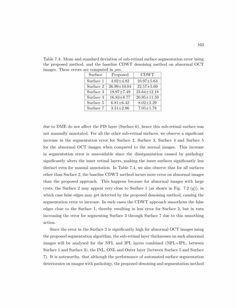
163

Table 7.4: Mean and standard deviation of sub-retinal surface segmentation error usingthe proposed method, and the baseline CDWT denoising method on abnormal OCTimages. These errors are computed in µm.

Surface Proposed CDWT

Surface 1 4.02±4.82 10.97±5.64

Surface 2 26.99±10.04 22.57±5.69

Surface 3 19.97±7.49 23.64±12.18

Surface 4 16.83±8.77 20.95±11.59

Surface 5 6.81±6.42 8.02±2.29

Surface 7 3.51±2.86 7.05±1.78

due to DME do not affect the PIS layer (Surface 6), hence this sub-retinal surface was

not manually annotated. For all the other sub-retinal surfaces, we observe a significant

increase in the segmentation error for Surface 2, Surface 3, Surface 4 and Surface 5

for the abnormal OCT images when compared to the normal images. This increase

in segmentation error is unavoidable since the disorganization caused by pathology

significantly alters the inner retinal layers, making the inner surfaces significantly less

distinct even for manual annotation. In Table 7.4, we also observe that for all surfaces

other than Surface 2, the baseline CDWT method incurs more error on abnormal images

than the proposed approach. This happens because for abnormal images with large

cysts, the Surface 2 may appear very close to Surface 1 (as shown in Fig. 7.2 (g)), in

which case false edges may get detected by the proposed denoising method, causing the

segmentation error to increase. In such cases the CDWT approach smoothens the false

edges close to the Surface 1, thereby resulting in less error for Surface 2, but in turn

increasing the error for segmenting Surface 3 through Surface 7 due to this smoothing

action.

Since the error in the Surface 2 is significantly high for abnormal OCT images using

the proposed segmentation algorithm, the sub-retinal layer thicknesses on such abnormal

images will be analyzed for the NFL and IPL layers combined (NFL+IPL, between

Surface 1 and Surface 3), the INL, ONL and Outer layer (between Surface 5 and Surface

7). It is noteworthy, that although the performance of automated surface segmentation

deteriorates on images with pathology, the proposed denoising and segmentation method

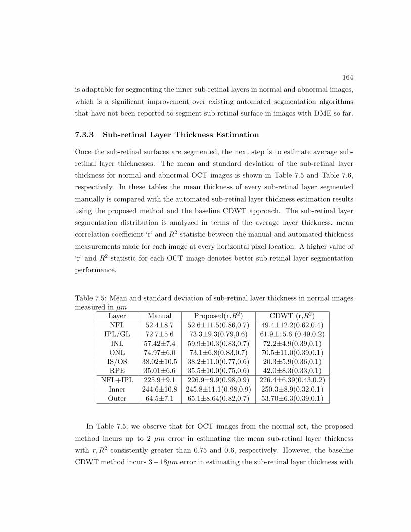
164

is adaptable for segmenting the inner sub-retinal layers in normal and abnormal images,

which is a significant improvement over existing automated segmentation algorithms

that have not been reported to segment sub-retinal surface in images with DME so far.

7.3.3 Sub-retinal Layer Thickness Estimation

Once the sub-retinal surfaces are segmented, the next step is to estimate average sub-

retinal layer thicknesses. The mean and standard deviation of the sub-retinal layer

thickness for normal and abnormal OCT images is shown in Table 7.5 and Table 7.6,

respectively. In these tables the mean thickness of every sub-retinal layer segmented

manually is compared with the automated sub-retinal layer thickness estimation results

using the proposed method and the baseline CDWT approach. The sub-retinal layer

segmentation distribution is analyzed in terms of the average layer thickness, mean

correlation coefficient ‘r’ and R2 statistic between the manual and automated thickness

measurements made for each image at every horizontal pixel location. A higher value of

‘r’ and R2 statistic for each OCT image denotes better sub-retinal layer segmentation

performance.

Table 7.5: Mean and standard deviation of sub-retinal layer thickness in normal imagesmeasured in µm.

Layer Manual Proposed(r,R2) CDWT (r,R2)

NFL 52.4±8.7 52.6±11.5(0.86,0.7) 49.4±12.2(0.62,0.4)IPL/GL 72.7±5.6 73.3±9.3(0.79,0.6) 61.9±15.6 (0.49,0.2)

INL 57.42±7.4 59.9±10.3(0.83,0.7) 72.2±4.9(0.39,0.1)ONL 74.97±6.0 73.1±6.8(0.83,0.7) 70.5±11.0(0.39,0.1)

IS/OS 38.02±10.5 38.2±11.0(0.77,0.6) 20.3±5.9(0.36,0.1)RPE 35.01±6.6 35.5±10.0(0.75,0.6) 42.0±8.3(0.33,0.1)

NFL+IPL 225.9±9.1 226.9±9.9(0.98,0.9) 226.4±6.39(0.43,0.2)Inner 244.6±10.8 245.8±11.1(0.98,0.9) 250.3±8.9(0.32,0.1)Outer 64.5±7.1 65.1±8.64(0.82,0.7) 53.70±6.3(0.39,0.1)

In Table 7.5, we observe that for OCT images from the normal set, the proposed

method incurs up to 2 µm error in estimating the mean sub-retinal layer thickness

with r,R2 consistently greater than 0.75 and 0.6, respectively. However, the baseline

CDWT method incurs 3−18µm error in estimating the sub-retinal layer thickness with

165

significantly low r,R2 metrics. The p-values for both the proposed segmentation system

and the baseline CDWT system is< 0.01. This analysis illustrates that although average

surface segmentation error between the proposed and baseline CDWT method was not

very high, the error in mean sub-retinal layer thickness and distribution of sub-retinal

layer thickness becomes significantly high.

Table 7.6: Mean and standard deviation of sub-retinal layer thickness in abnormalimages measured in µm.

Layer Manual Proposed(r,R2) CDWT(r,R2)

NFL+IPL 111.5±15.9 129.4±19.7(0.78,0.6) 135.6±29.7(0.75,0.6)INL 62.7±10.6 60.9±15.0(0.73,0.5) 76.9±14.5(0.36,0.1)ONL 89.9±15.3 81.0±13.9(0.71,0.5) 70.9±11.4(0.23,0.1)

Inner 265.6±33.1 274.9±34.6(0.92,0.8) 274.0±61.3(0.90,0.8)Outer 60.9±8.44 57.4±14.4(0.74,0.6) 49.7±10.6(0.32,0.1)

In Table 7.6, we observe that the proposed method incurs 2−18µm error in estimat-

ing the mean sub-retinal layer thickness with r,R2 statistics consistently more than 0.7

and 0.5, respectively. On the other hand, the baseline CDWT method incurs 12−24µm

error for mean thickness estimation with (r,R2) statistics ranging from (0.3, 0.1) to

(0.9, 0.8).

7.3.4 Thickness Map Analysis

Finally, the segmented sub-retinal thickness distributions obtained for each OCT image

are combined for all images from a particular OCT stack to generate thickness maps.

The sub-retinal layer thickness maps for an abnormal image stack with cystic DME are

shown in Fig. 7.5.

Fig. 7.5 contains the OCT scan shown in Fig. 7.2. In Fig. 7.5 we observe that

the thickness maps of the proposed method resemble the manually segmented thickness

maps more than the baseline CDWT method.

It is important to note that the thickness maps of INL and ONL vary significantly

for normal and abnormal OCT stacks. This difference is illustrated in Fig. 7.6, where

manually segmented thickness maps from two normal and two abnormal OCT stacks

each are shown. In Fig. 7.6 thickness maps of the INL in normal images demonstrate

166

thinning at the central fovea while ONL in normal images demonstrate a relatively

thick layer at the fovea with the maximum thickness below 120µm. This observation is

intuitive. However, in the INL maps for abnormal images with DME, the thin INL at

central fovea disappears, and the ONL either appears irregular or the thickness exceeds

200 µm. These changes to the INL and ONL thickness maps occur due to the sub-

retinal cysts that form or the disorganization that occurs due to pathology. Since these

differences in INL and ONL thickness maps are evident, these thickness maps could in

turn be used as an indicator of disease severity or risk to visual acuity in future clinical

studies.

From the previous experiments we have observe that the proposed sub-retinal surface

segmentation method achieves ‘r > 0.8’ (p < 0.001) for segmenting thickness maps of

INL and ONL from normal OCT stacks, but this accuracy deteriorates to 0.7 (p < 0.001)

for thickness maps of INL and ONL in abnormal OCT stacks. Although the automated

segmentation error in images with pathology is unavoidable, we observe the manual

and automated thickness maps to identify some other features that may be strongly

correlated to the manual thickness maps.

In Fig. 7.7, we analyze the area of irregularities in the INL and ONL thickness maps

from DME patients. As observed in Fig. 7.6, the INL and ONL in abnormal images

demonstrate abnormally high thickness, which appear to be plateau regions in their

respective thickness maps. The contoured area of these plateau regions in INL and

ONL extracted using the manual segmentations, proposed method and the Baseline

CDWT approaches are shown in Fig. 7.7.

To obtain the contoured areas of irregular thickness from the manually and auto-

mated segmented thickness maps, the first step is the scale all the thickness maps in

the minimum variation range that is obtained using the automated or manual methods.

This means that if the thicknesses obtained by manual and automated segmentations

range in [0, 120], and [0,200], respectively, then both thickness maps are scaled in

[0,120]. Next, the area of the irregular plateau regions are obtained by low-pass filtering

the scaled thickness map surface with an average [25x25] filter, followed by subtraction

of the filtered surface from the actual and thresholding using Otsu’s threshold function.

Among all the regions that get extracted, the regions that lie towards the center of the

surfaces with the large areas, and maximum surface pixel strength (that is indicative of

167

high thickness) are selected as the irregular areas. Thus, such irregular region areas that

are extracted from the INL and ONL of manually and automated segmented thickness

maps by the proposed and baseline CDWT approach and extracted and compared.

In Fig. 7.7 we observe that the combined area of irregular plateau regions extracted

from the thickness maps of INL and ONL from manual segmentations is 7710 pixel2,

while the combined area of from the same layers obtained by the proposed method

and baseline CDWT method are 7336 pixel2 and 4321 pixel2, respectively. Here, we

observe that the manual segmentation captures the irregularity due to pathology in the

INL and the ONL, while the automated segmentations capture this irregularity in the

INL only. However, the combined area of irregularity from the INL and ONL obtained

manually closely matches the area obtained by the proposed approach. On comparing

the combined irregularity areas obtained in INL and ONL maps for the 15 OCT stacks

under analysis, we observe that the proposed method and the baseline CDWT methods

have [r,R2] statistics of [0.99,0.98] and [0.92, 0.85], respectively, with (p < 0.001).

This analysis indicates that although automated segmentation on sub-retinal surfaces

in abnormal OCT image stacks with DME has a lower correlation coefficient to the

manual segmentations than normal images stacks, the area of irregularity obtained from

thickness maps of the INL and ONL correlate highly with their manually segmented

counterparts. This observation encourages the use of automated inner sub-retinal layer

segmentation systems to clinically analyze pathology progression over time. Also, the

combined area of irregularity in the INL and ONL can be assessed as an indicator for

DME severity and visual acuity over time in future efforts.


In this chapter we have proposed a novel automated segmentation system that denoises

and segments 7 sub-retinal surfaces and 6 sub-retinal layers in the retinal microstructure

for normal OCT images from healthy patients and in abnormal images from patients

with DME in less than 35 seconds per image. The proposed system is implemented on a

2.53 GHz Intel Core i3 and 3 GB RAM Laptop system using MATLAB. Also, the sub-

retinal layer thickness distributions from all images belonging to an OCT image stack

are combined to generate thickness maps that aid analysis and assessment of DME with

168

time.

We analyze the performance of OCT speckle noise removal using the proposed

Wiener deconvolution method that estimates noise parameters using a Fourier-domain

structural error metric defined in [137]. The proposed denoising method is compared to

wavelet-transform based CDWT method used in [129]. Our analysis shows that the pro-

posed Fourier domain-based denoising method improves the image SNR by more than

12dB, and it retains the sub-retinal surface edges within the retinal microstructure while

suppressing the speckle noise significantly in the image background, thereby incurring

a PSNR of about 23.5dB. The CDWT method on the other hand conserves the sub-

retinal structure of the image foreground and background by smoothing the sub-retinal

edges, thereby achieving a high PSNR of about 28dB but an SNR enhancement of less

than 5dB. Further analysis shows that the CDWT denoising method incurs more error

while automated segmentation of sub-retinal surfaces when compared to the proposed

denoising method. Thus, for the proposed sub-retinal surface and layer segmentation

algorithm, the proposed Fourier-domain based denoising method is better suited.

The proposed sub-retinal surface segmentation algorithm exhibits significant relia-

bility is extracting sub-retinal layer thicknesses for normal and abnormal OCT image

stacks. These sub-retinal layer thicknesses can then be used to generate thickness maps

for healthy eyes and for DME patients. The structure and thickness of the INL and

ONL in healthy and abnormal OCT image stacks is observed to vary significantly. For

OCT image stacks with DME, the INL and ONL demonstrate irregular plateau regions

that appear due to underlying cysts and sub-retinal layer disorganizations. The pro-

posed segmentation system is capable of capturing the combined area of irregularities in

INL and ONL of abnormal image stacks with ‘r=0.99’. Future efforts will be focused on

further assessment of this combined area of irregularity in the INL and ONL for DME

patients over time and for evaluating the correlation of this metric to visual acuity.

Another key observation is that the segmentation performance of the proposed de-

noising and segmentation algorithm deteriorates significantly from normal OCT images

to abnormal ones, i.e., error in mean sub-retinal thickness estimation is 0−2µm for for-

mal images and 2−18µm for abnormal images. However, the baseline CDWT denoising

method followed by the proposed segmentation deteriorates significantly in estimating

the distribution of sub-retinal thicknesses (low ‘r’ value), but the estimation of mean

169

sub-retinal layer thickness does not deteriorate as much, i.e., error in mean sub-retinal

thickness estimation is 3−18µm for formal images and 12−24µm for abnormal images.

This observation strengthens the fact that the proposed segmentation algorithm is ro-

bust and can be combined with other denoising approaches to estimate mean sub-retinal

layer thickness in normal and abnormal images.

The estimation of irregular area on the thickness maps of INL and ONL using the

proposed denoising and baseline CDWT methods followed by the proposed segmentation

demonstrate high correlation with the area estimated from the manually segmented

surfaces (r > 0.92, p < 0.001). This observation encourages further analysis of this

irregular area metric for DME patients in future works.

170

(a) (b) (c)

(d) (e) (f)

(g) (h)

Figure 7.2: Steps for the proposed iterative multi-resolution segmentation algorithm onan abnormal OCT image. (a) Denoised image by the proposed method (Id). (b)ImageI1 obtained after high-pass filtering in iteration k = 1. Thresholding this image resultsin the detection of Surface 1 and the choroidal segment(c) Negative source image 1− Idin iteration k = 2 within the region of interest marked by G2 that extends betweenthe Surface 1 and the choroid segment.(d) Image obtained after high-pass filtering andthresholding the image in (c) in iteration k = 2. The region with maximum majoraxis length is extracted in image Ir2 . The top surface of this region is Surface 5, andthe bottom surface is Surface 7. (e) Image obtained in iteration k = 4 after high-passfiltering and thresholding. The region with maximum major axis length is selected inimage Ir4 , and the bottom surface of this region is Surface 4. Two more iterations areperformed to extract all 7 surfaces. (f) Automated segmentation achieved at the end of 6iteration steps by the proposed method. (g) Manually marked surfaces. (h) Automatedsegmentation achieved using baseline CDWT approach for denoising followed by theproposed segmentation algorithm.

171

Figure 7.3: Sub-retinal layer thickness maps for a normal OCT image stack. The firstcolumn of images represents thickness maps generated by interpolating the sub-retinalthickness of each layer obtained by manual annotation. The second column of imagesrepresents the thickness maps obtained by the proposed denoising and segmentationalgorithms. The third column of images represents the thickness maps obtained by thebaseline CDWT denoising method followed by the proposed segmentation algorithm.For each segmented thickness map obtained by the proposed denoising method andthe baseline CDWT method, the mean sub-retinal layer thickness and the correlationcoefficient ‘r’ of automated thickness distribution with respect to the manual thicknessesare provided.

172

(a) (b) (c)

(d)

Figure 7.4: Example of automated OCT image denoising. (a) Noisy image (I), (b) Theforeground region lies within the region bordered by the red boundary. All other regionsare the background. (c) Denoised image by CDWT method. (d) Denoised image by theproposed method.

173

Figure 7.5: Sub-retinal layer thickness maps for an abnormal OCT image stack. The firstcolumn of images represents thickness maps generated by manual annotation. The sec-ond column of images represents the thickness maps obtained by the proposed method.The third column of images represents the thickness maps obtained by the baselineCDWT method. For each segmented thickness map obtained by the proposed denois-ing method and the baseline CDWT method, the mean sub-retinal layer thickness andthe correlation coefficient ‘r’ of automated thickness distribution with respect to themanual thicknesses are provided.

174

Figure 7.6: Difference between thickness maps of the INL and ONL in normal andabnormal images with DME.

Figure 7.7: Irregular plateau regions observed in INL and ONL of the segmented ab-normal OCT image stack. First second and third columns indicate thickness mapssegmented manually, by the proposed method and by the baseline CDWT methods,respectively. The combined area of irregularity extracted from the INL and ONL fromthe manual thickness maps, are highly correlated to the combined area of INL and ONLfrom the automated segmentation methods.

Chapter 8

Conclusions and Future Work

8.1 Conclusions

In this thesis we have presented algorithms for automated information extraction from

multi-modal ophthalmic images pertaining to the human retina. These algorithms are

aimed at translating the cognitive understanding of specialists into computer intelli-

gence. Using domain knowledge and theoretical concepts of digital image processing

and machine learning, we have developed and optimized algorithms to segment the im-

ages into regions of interest and detect the presence of abnormalities due to pathologies

in them. The algorithms presented here are both robust to variations in image due to

the imaging cameras or pathologies, and computationally less complex when compared

to existing algorithms. All the segmentation and pathology detection algorithms pre-

sented in this thesis have been analyzed using data sets that were manually annotated

by specialists. The conclusions from three categories of contributions made in this thesis

are as follows.

8.1.1 Automated Segmentation of Retinal Anatomical Regions in Fun-

dus Images

In this thesis, we have presented two algorithms for automated segmentation of blood

vessels from fundus images and one algorithm for automated detection of the OD bound-

ary and vessel origin. The first algorithm for automated blood vessel segmentation uses

175

176

high-pass filtering and morphology based approach to detect major vessel regions fol-

lowed by a classification-based approach to detect the fine blood vessels that are then

added to the major vessels. For accurate vessel pixel identification, we analyze intensity-

based pixel features to identify a most discriminating set of 8 features that classify a

vessel pixel from a background non-vessel pixel. Vessel classification is done using a

2-Gaussian GMM classifier that ensures low computational complexity. This algorithm

can be effectively used for detecting NVD, RoP vein occlusions and other vessel related

retinal abnormalities.

The second algorithm for blood vessel segmentation uses an iterative approach to

identify fine vessel segments and adding them to the existing vessel estimates. This

algorithm utilizes a stopping criterion based on the rate of vessel-pixel addition to

extract the best vessel estimate. Since this algorithm identifies sparse vessel segments

in each iteration, it can be useful for automated detection of NVE caused by PDR,

where vessel-like segments appear in close vicinity of the blood vessels.

The algorithm for OD boundary and vessel origin detection presented here is capable

of detection the OD region in normal images and in images with abnormalities. This

rule-based algorithm can be useful for cup-to-disc ratio measurements for patients with

Glaucoma, and for detecting pathologies like NVD that affect the OD region.

8.1.2 Automated DR screening systems

Automated screenings of fundus images for DR require background detection modules

for segmentation and removal of the blood vessels and the OD region in the initial stage.

Next, in the foreground region, abnormal regions are detected as bright lesion and red

lesions followed by classification of these lesion regions. The NPDR screening system

presented in this thesis detects the most discriminating structure based feature set for

classification of the lesion regions. Such a screening systems can reduce the number of

images that need subsequent manual assessment by 50%.

Automated screening for PDR is a more challenging problem than NPDR, since the

fine vessel-like abnormalities appear in close vicinity of the blood vessels that can be

mistaken for blood vessel regions. Hence, the iterative vessel segmentation approach

followed by structure-based decision making can detect these new-vessel abnormalities

at the OD region and elsewhere.

177

8.1.3 Automated Segmentation of OCT images

Automated segmentation algorithms of sub-retinal layers for normal and pathological

OCT images with DME have been presented in this thesis. These algorithms estimate

the thickness of the sub-retinal layers and demonstrate the change caused by pathology.

Such algorithms can aid quicker clinical assessments regarding the effectiveness of DME

treatment over time.

8.2 Future Work

The algorithms presented in this thesis have been aimed at detecting abnormalities that

can lead to acquired blindness in diabetic patients. Future work will be aimed at extend-

ing these algorithms to non-diabetic vision threatening pathologies such as hypertensive

retinopathy. The directions for future work pertaining to each segmentation algorithm

or screening system presented in this thesis are as follows.

• For the blood vessel segmentation algorithm using classification-based approach,

the performance of other classifiers for vessel pixel identification can be analyzed.

Also, using the Expectation-Maximization algorithm, GMM classifiers with more

than 2 Gaussians can be trained for identifying fine vessel pixels. Also, the impact

of the segmented vessel region for detection of NVD can be analyzed.

• For the iterative blood vessel segmentation algorithm, extensions of the proposed

algorithm for blood vessel segmentation in wide-field or Optos images with more

than 200o FOV can be analyzed. Also, algorithms that use the presented methods

of the blood vessel segmentation for detecting blood vessel properties such as

tortuosity, arterio-venular ratio, vessel thickness and branching patterns can be

developed. The effectiveness of the iterative blood vessel segmentation algorithm

for NVE detection can be further analyzed.

• The automated OD segmentation algorithm presented in this thesis can be used

with cup-to-disk ratio measurement modules to automatically assess the severity

of Glaucoma. Also, the detection modules for the macula based on its distance

from the OD region can be developed for severity analysis of maculopathy.

178

• The automated NPDR screening system can be analyzed on more images from

locally acquired image sets for further performance verification. Also, the auto-

mated PDR detection module can be combined with the NPDR detection modules

for a complete screening system for DR. Additionally, extensions to the existing

DR screening system on wide field images can be analyzed.

• The automated PDR detection algorithms can be further fine-tuned using anno-

tated training data sets. Structure-based features can be ranked in their order of

their discriminating performance for detecting the laser scars, fibrosed tissues and

NVE regions. Pixel-based performance evaluation for detecting fine vessel-like

abnormalities can be done. Based on the abnormal vessel regions detected, the

severity of PDR can also be analyzed for each fundus image.

• The proposed OCT segmentation system can be used to clinically asses the change

in the inner sub-retinal layers for DME patients over time. Also, this system can

be used on patients with other retinal pathologies such as Macular Telangiectasia

(Mactel), maculopathy etc.

References

[1] K. Doi, “Computer-aided diagnosis in medical imaging: Historical review, current

status and future potential,” Computerized medical imaging and graphics, vol. 31,

no. 4, pp. 198–211, 2007.

[2] C. for Disease Control and Prevention, “The economic impact of adult visual

disorders in the united states.” [Online]. Available: http://www.cdc.gov/

visionhealth/publications/economic impact.htm

[3] S. Roychowdhury, D. Koozekanani, and K. Parhi, “Dream: Diabetic retinopa-

thy analysis using machine learning,” IEEE Journal of Biomedical and Health

Informatics, 2013.

[4] M. D. Abramoff, M. Niemeijer, and S. R. Russell, “Automated detection of dia-

betic retinopathy: barriers to translation into clinical practice,” in Expert Review

of Medical Devices, vol. 7, no. 2, 2010, pp. 287–296.

[5] CDC, “Diabetic retinopathy. atlanta, ga: National for chronic disease

prevention and health promotion.” March 23,2011. [Online]. Available:

http://www.cdc.gov/visionhealth/pdf/factsheet.pdf

[6] H. M. Pakter, S. C. Fuchs, M. K. Maestri, L. B. Moreira, L. M. Dei Ricardi,

V. F. Pamplona, M. M. Oliveira, and F. D. Fuchs, “Computer-assisted methods

to evaluate retinal vascular caliber: What are they measuring?” Investigative

Ophthalmology and Visual Science, vol. 52, no. 2, pp. 810–815, 2011.

179

http://www.cdc.gov/visionhealth/publications/economic_impact.htm

http://www.cdc.gov/visionhealth/publications/economic_impact.htm

http://www.cdc.gov/visionhealth/pdf/factsheet.pdf

180

[7] K. Kotliar, E. Nagel, W. Vilser, S.-F. Seidova, and I. Lanzl, “Microstructural

alterations of retinal arterial blood column along the vessel axis in systemic hy-

pertension,” Investigative Ophthalmology and Visual Science, vol. 51, no. 4, pp.

2165–2172, 2010.

[8] A. Kochkorov, K. Gugleta, C. Zawinka, R. Katamay, J. Flammer, and S. Orgul,

“Short-term retinal vessel diameter variability in relation to the history of cold

extremities,” Investigative Ophthalmology and Visual Science, vol. 47, no. 9, pp.

4026–4033, 2006.

[9] E. Nagel, W. Vilser, and I. Lanzl, “Age, blood pressure, and vessel diameter as fac-

tors influencing the arterial retinal flicker response,” Investigative Ophthalmology

and Visual Science, vol. 45, no. 5, pp. 1486–1492, 2004.

[10] S. Roychowdhury, D. D. Koozekanani, and K. K. Parhi, “Screening fundus images

for diabetic retinopathy,” in 2012 Conference Record of the Forty Sixth Asilomar

Conference on Signals, Systems and Computers (ASILOMAR), 2012, pp. 1641–

1645.

[11] R. Perfetti, E. Ricci, D. Casali, and G. Costantini, “Cellular neural networks with

virtual template expansion for retinal vessel segmentation,” IEEE Transactions

on Circuits and Systems II: Express Briefs, vol. 54, no. 2, pp. 141–145, 2007.

[12] M. Fraz, P. Remagnino, A. Hoppe, B. Uyyanonvara, A. Rudnicka, C. Owen, and

S. Barman, “An ensemble classification-based approach applied to retinal blood

vessel segmentation,” IEEE Transactions on Biomedical Engineering, vol. 59,

no. 9, pp. 2538–2548, 2012.

[13] D. Marin, A. Aquino, M. Gegundez-Arias, and J. Bravo, “A new supervised

method for blood vessel segmentation in retinal images by using gray-level and mo-

ment invariants-based features,” IEEE Transactions on Medical Imaging, vol. 30,

no. 1, pp. 146–158, 2011.

[14] M. Fraz, P. Remagnino, A. Hoppe, B. Uyyanonvara, A. Rudnicka, C. Owen, and

S. Barman, “Blood vessel segmentation methodologies in retinal images a survey,”

181

Computer Methods and Programs in Biomedicine, vol. 108, no. 1, pp. 407 – 433,

2012.

[15] A. Hoover, V. Kouznetsova, and M. Goldbaum, “Locating blood vessels in reti-

nal images by piecewise threshold probing of a matched filter response,” IEEE

Transactions on Medical Imaging, vol. 19, pp. 203–210, 2000.

[16] R. Rangayyan, F. Oloumi, F. Oloumi, P. Eshghzadeh-Zanjani, and F. Ayres, “De-

tection of blood vessels in the retina using gabor filters,” in Canadian Conference

on Electrical and Computer Engineering, 2007, pp. 717–720.

[17] A. Mendonca and A. Campilho, “Segmentation of retinal blood vessels by combin-

ing the detection of centerlines and morphological reconstruction,” IEEE Trans-

actions on Medical Imaging, vol. 25, no. 9, pp. 1200–1213, 2006.

[18] M. Miri and A. Mahloojifar, “Retinal image analysis using curvelet transform

and multistructure elements morphology by reconstruction,” IEEE Transactions

on Biomedical Engineering, vol. 58, no. 5, pp. 1183–1192, 2011.

[19] K. A. Vermeer, F. M. Vos, H. G. Lemij, and A. M. Vossepoel, “A model based

method for retinal blood vessel detection,” Computers in Biology and Medicine,

vol. 34, no. 3, pp. 209–219, 2004.

[20] B. Lam and H. Yan, “A novel vessel segmentation algorithm for pathological retina

images based on the divergence of vector fields,” IEEE Transactions on Medical

Imaging, vol. 27, no. 2, pp. 237–246, 2008.

[21] B. Lam, Y. Gao, and A.-C. Liew, “General retinal vessel segmentation using

regularization-based multiconcavity modeling,” IEEE Transactions on Medical

Imaging, vol. 29, no. 7, pp. 1369–1381, 2010.

[22] X. Jiang and D. Mojon, “Adaptive local thresholding by verification-based mul-

tithreshold probing with application to vessel detection in retinal images,” IEEE

Transactions on Pattern Analysis and Machine Intelligence, vol. 25, no. 1, pp.

131–137, 2003.

182

[23] B. Al-Diri, A. Hunter, and D. Steel, “An active contour model for segmenting and

measuring retinal vessels,” IEEE Transactions on Medical Imaging, vol. 28, no. 9,

pp. 1488–1497, 2009.

[24] A. Budai, G. Michelson, and J. Hornegger, “Multiscale blood vessel segmentation

in retinal fundus images,” Proc. Bildverarbeitung fr die Med., pp. 261–265, March

2010.

[25] A. Budai, R. Bock, A. Maier, J. Hornegger, and G. Michelson, “Robust vessel

segmentation in fundus images,” International Journal of Biomedical Imaging,

no. 154860, 2013.

[26] M. Niemeijer, J. Staal, B. van Ginneken, M. Loog, and M. D. Abramoff, “Com-

parative study of retinal vessel segmentation methods on a new publicly available

database,” Proc. SPIE 5370, Medical Imaging, vol. 5370, pp. 648–656, 2004.

[27] J. Staal, M. Abramoff, M. Niemeijer, M. Viergever, and B. van Ginneken, “Ridge-

based vessel segmentation in color images of the retina,” IEEE Transactions on

Medical Imaging, vol. 23, no. 4, pp. 501–509, 2004.

[28] J. Soares, J. Leandro, R. Cesar, H. Jelinek, and M. Cree, “Retinal vessel segmen-

tation using the 2-D Gabor wavelet and supervised classification,” IEEE Trans-

actions on Medical Imaging, vol. 25, no. 9, pp. 1214–1222, 2006.

[29] E. Ricci and R. Perfetti, “Retinal blood vessel segmentation using line operators

and support vector classification,” IEEE Transactions on Medical Imaging, vol. 26,

no. 10, pp. 1357–1365, 2007.

[30] K. U. Research, “Chase db1,” January 2011. [Online]. Available: http:

//blogs.kingston.ac.uk/retinal/chasedb1/.

[31] A. Frame, P. Undrill, M. Cree, J. Olson, K. McHardy, P. Sharp, and J. Forrester,

“A comparison of computer based classification methods applied to the detection

of microaneurysms in ophthalmic fluorescein angiograms,” Comput. Biol. Med.,

vol. 28, pp. 225–238, 1998.

http://blogs.kingston.ac.uk/retinal/chasedb1/.

http://blogs.kingston.ac.uk/retinal/chasedb1/.

183

[32] V. Cherkassky and F. Mullier, “Learning from data,” John Wiley and sons, New

York, 1998.

[33] H. Peng, F. Long, and C. Ding, “Feature selection based on mutual information

criteria of max-dependency, max-relevance, and min-redundancy,” Pattern Analy-

sis and Machine Intelligence, IEEE Transactions on, vol. 27, no. 8, pp. 1226–1238,

Aug 2005.

[34] K. Goatman, A. Fleming, S. Philip, G. Williams, J. Olson, and P. Sharp, “Detec-

tion of new vessels on the optic disc using retinal photographs,” IEEE Transac-

tions on Medical Imaging, vol. 30, no. 4, pp. 972–979, 2011.

[35] C. M. Wilson, K. D. Cocker, M. J. Moseley, C. Paterson, S. T. Clay, W. E.

Schulenburg, M. D. Mills, A. L. Ells, K. H. Parker, G. E. Quinn, A. R. Fielder, and

J. Ng, “Computerized analysis of retinal vessel width and tortuosity in premature

infants,” Investigative Ophthalmology and Visual Science, vol. 49, no. 8, pp. 3577–

3585, 2008.

[36] A. Karperien, H. F. Jelinek, J. J. Leandro, J. V. Soares, R. M. Cesar Jr, and

A. Luckie, “Automated detection of proliferative retinopathy in clinical practice,”

Clinical ophthalmology (Auckland, NZ), vol. 2, no. 1, p. 109, 2008.

[37] T. Teng, M. Lefley, and D. Claremont, “Progress towards automated diabetic

ocular screening: A review of image analysis and intelligent systems for diabetic

retinopathy,” Medical and Biological Engineering and Computing, vol. 40, pp.

2–13, 2002.

[38] R. C. Gonzalez and R. E. Woods, Digital Image Processing, 2nd ed. Boston,

MA, USA: Addison-Wesley Longman Publishing Co., Inc., 1992.

[39] R. A. Abdel-Ghafar and T. Morris, “Progress towards automated detection and

characterization of the optic disc in glaucoma and diabetic retinopathy,” Medical

Informatics and the Internet in Medicine, vol. 32, no. 1, pp. 19–25, March 2007.

[40] D. Koozekanani, K. Boyer, C. Roberts, and S. Katz, “Tracking the optic nerve

head in oct video using dual eigenspaces and an adaptive vascular distribution

184

model,” in Proceedings of the 2001 IEEE Computer Society Conference on Com-

puter Vision and Pattern Recognition, 2001., vol. 1, 2001, pp. I–934–I–941 vol.1.

[41] R. J. Qureshi, L. Kovacs, B. Harangi, B. Nagy, T. Peto, and A. Hajdu, “Combining

algorithms for automatic detection of optic disc and macula in fundus images,”

Computer Vision and Image Understanding, vol. 116, no. 1, pp. 138 – 145, 2012.

[42] A. Aquino, M. Gegundez-Arias, and D. Marin, “Detecting the optic disc boundary

in digital fundus images using morphological, edge detection, and feature extrac-

tion techniques,” IEEE Transactions on Medical Imaging, vol. 29, no. 11, pp. 1860

–1869, nov. 2010.

[43] C. Sinthanayothin, J. F. Boyce, H. L. Cook, and T. H.Williamson, “Automated

localisation of the optic disk, fovea, and retinal blood vessels from digital colour

fundus images,” Br. J. Ophthalmol, vol. 83, no. 8, pp. 902–910, 1999.

[44] A. Hoover, , and M. Goldbaum, “Locating the optic nerve in retinal image using

the fuzzy convergence of bood vessels,” IEEE Transactions on Medical Imaging,

vol. 22, August 2003.

[45] F. ter Haar, “Automatic localization of the optic disc in digital colour images of

the human retina,” M.S. Thesis, 2005.

[46] A. Osareh, M. Mirmehdi, B. Thomas, and R. Markham, “Classification and lo-

calisation of diabetic-related eye disease,” in Computer Vision ECCV 2002, ser.

Lecture Notes in Computer Science, vol. 2353. Springer Berlin / Heidelberg,

2006, pp. 325–329.

[47] M. Lalonde, M. Beaulieu, and L. Gagnon, “Fast and robust optic disc detection

using pyramidal decomposition and hausdorff-based template matching,” IEEE

Transactions on Medical Imaging, vol. 20, no. 11, pp. 1193 –1200, Nov. 2001.

[48] H. Yu, S. Barriga, C. Agurto, S. Echegaray, M. Pattichis, G. Zamora, W. Bauman,

and P. Soliz, “Fast localization of optic disc and fovea in retinal images for eye

disease screening,” Medical Imaging 2011: Computer-Aided Diagnosis, vol. 7963,

no. 1, p. 796317, 2011.

185

[49] J. Lowell, A. Hunter, D. Steel, A. Basu, R. Ryder, E. Fletcher, and L. Kennedy,

“Optic nerve head segmentation,” IEEE Transactions on Medical Imaging, vol. 23,

no. 2, pp. 256 –264, Feb. 2004.

[50] R. Rangayyan, X. Zhu, and F. Ayres, “Detection of the optic disc in images

of the retina using gabor filters and phase portrait analysis,” in 4th European

Conference of the International Federation for Medical and Biological Engineering,

2009, vol. 22, pp. 468–471.

[51] A. Salazar-Gonzalez, Y. Li, and X. Liu, “Optic disc segmentation by incorpo-

rating blood vessel compensation,” in IEEE Third International Workshop On

Computational Intelligence In Medical Imaging (CIMI), 2011, pp. 1–8.

[52] D. Welfer, J. Scharcanski, C. M. Kitamura, M. M. Dal Pizzol, L. W. B. Ludwig,

and D. R. Marinho, “Segmentation of the optic disk in color eye fundus images

using an adaptive morphological approach,” Comput. Biol. Med., vol. 40, no. 2,

pp. 124–137, Feb. 2010.

[53] A. M. Mendonca, A. Sousa, L. Mendonca, and A. Campilho, “Automatic local-

ization of the optic disc by combining vascular and intensity information,” Com-

puterized medical imaging and graphics : the official journal of the Computerized

Medical Imaging Society, vol. 37(5-6), pp. 409–417, Sept 2013.

[54] M. Goldbaum, S. Moezzi, A. Taylor, S. Chatterjee, J. Boyd, E. Hunter, and

R. Jain, “Automated diagnosis and image understanding with object extraction,

object classification, and inferencing in retinal images,” vol. 3, Sept. 1996, pp. 695

–698 vol.3.

[55] M. Niemeijer, J. Staal, B. van Ginneken, M. Loog, and M. D. Abramoff, “Com-

parative study of retinal vessel segmentation methods on a new publicly available

database,” Medical Imaging 2004: Image Processing, vol. 5370, no. 1, pp. 648–656,

2004.

[56] M. Niemeijer, M. Abramoff, and B. van Ginneken, “Segmentation of the optic

disc, macula and vascular arch in fundus photographs,” IEEE Transactions on

Medical Imaging, vol. 26, no. 1, pp. 116 –127, Jan. 2007.

186

[57] S. Morales, V. Naranjo, J. Angulo, and M. Alcaniz, “Automatic detection of optic

disc based on pca and mathematical morphology,” IEEE Transactions on Medical

Imaging, vol. 32, no. 4, pp. 786–796, April 2013.

[58] “Gnu image manipulation program,” January 1996. [Online]. Available:

http://www.gimp.org/downloads/.

[59] J. Staal, M. Abramoff, M. Niemeijer, M. Viergever, and B. van Ginneken, “Ridge

based vessel segmentation in color images of the retina,” IEEE Transactions on

Medical Imaging, vol. 23, pp. 501–509, 2004.

[60] T. Kauppi, V. Kalesnykiene, J.-K. Kmrinen, L. Lensu, I. Sorr, A. Raninen,

R. Voutilainen, H. Uusitalo, H. Klviinen, and J. Pietil, “Diaretdb1 diabetic

retinopathy database and evaluation protocol,” Proc. of the 11th Conf. on Medical

Image Understanding and Analysis (MIUA2007), pp. 61–65, 2007.

[61] T. Kauppi, V. Kalesnykiene, J.-K. Kamarainen, L. Lensu, I. Sorri, H. Uusitalo,

H. Klviinen, and J. Pietil, “Diaretdb0: Evaluation database and methodology for

diabetic retinopathy algorithms,” Lappeenranta University of Technology, Fin-

land, Tech. Rep., 2006.

[62] “Methods to evaluate segmentation and indexing techniques in the field

of retinal ophthalmology.” Accessed Sept 23, 2011. [Online]. Available:

http://messidor.crihan.fr/download-en.php

[63] A. Sopharak, B. Uyyanonvara, S. Barman, and T. H. Williamson, “Automatic

detection of diabetic retinopathy exudates from non-dilated retinal images using

mathematical morphology methods,” Computerized Medical Imaging and Graph-

ics, vol. 32, no. 8, pp. 720 – 727, 2008.

[64] T. Walter, J.-C. Klein, P. Massin, and A. Erginay, “A contribution of image

processing to the diagnosis of diabetic retinopathy-detection of exudates in color

fundus images of the human retina,” IEEE Transactions on Medical Imaging,

vol. 21, no. 10, pp. 1236–1243, 2002.

http://www.gimp.org/downloads/.

http://messidor.crihan.fr/download-en.php

187

[65] J. Seo, K. Kim, J. Kim, K. Park, and H. Chung, “Measurement of ocular torsion

using digital fundus image,” in 26th Annual International Conference of the IEEE

Engineering in Medicine and Biology Society, vol. 1, 2004, pp. 1711–1713.

[66] G. Kande, P. Subbaiah, and T. Savithri, “Segmentation of exudates and optic

disk in retinal images,” in Sixth Indian Conference on Computer Vision, Graphics

Image Processing, 2008, pp. 535–542.

[67] K. Stapor, A. Switonski, R. Chrastek, and G. Michelson, “Segmentation of fundus

eye images using methods of mathematical morphology for glaucoma diagnosis,”

in International Conference on Computational Science, 2004, pp. 41–48.

[68] C. Lupascu, D. Tegolo, and L. Di Rosa, “Automated detection of optic disc lo-

cation in retinal images,” in IEEE International Symposium on Computer-Based

Medical Systems, 2008, pp. 17–22.

[69] Y. Zeng, D. Samaras, W. Chen, and Q. Peng, “Topology cuts: A novel min-

cut/max-flow algorithm for topology preserving segmentation in n-d images,”

Comput. Vis. Image Underst., vol. 112, no. 1, pp. 81–90, Oct. 2008.

[70] Y. Boykov and G. Funka-Lea, “Graph cuts and efficient n-d image segmentation,”

International Journal of Computer Vision, vol. 70, no. 2, pp. 109–131, 2006.

[71] S. Lu and J.-H. Lim, “Automatic optic disc detection from retinal images by a

line operator,” IEEE Transactions on Biomedical Engineering, vol. 58, no. 1, pp.

88–94, 2011.

[72] S. Ravishankar, A. Jain, and A. Mittal, “Automated feature extraction for early

detection of diabetic retinopathy in fundus images,” in IEEE Conference on Com-

puter Vision and Pattern Recognition, 2009, pp. 210–217.

[73] M. Niemeijer, M. D. Abrmoff, and B. van Ginneken, “Fast detection of the optic

disc and fovea in color fundus photographs,” Medical Image Analysis, vol. 13,

no. 6, pp. 859 – 870, 2009.

188

[74] A. Dehghani, H. Moghaddam, and M.-S. Moin, “Optic disc localization in reti-

nal images using histogram matching,” EURASIP Journal on Image and Video

Processing, vol. 2012, no. 1, pp. 1–11, 2012.

[75] A.-H. Abdel-Razik Youssif, A. Ghalwash, and A. Abdel-Rahman Ghoneim, “Op-

tic disc detection from normalized digital fundus images by means of a vessels’

direction matched filter,” IEEE Transactions on Medical Imaging, vol. 27, no. 1,

pp. 11 –18, Jan. 2008.

[76] American Diabetes Association, “Data from the 2011 national diabetes

fact sheet.” Jan. 26, 2011. [Online]. Available: http://www.diabetes.org/

diabetes-basics/diabetes-statistics/

[77] S. Garg and R. M. Davis, “Diabetic retinopathy screening update,” CliniCal Di-

abetes, vol. 27, no. 4, pp. 140–145, 2009.

[78] J. Cuadros and G. Bresnick, “Eyepacs: An adaptable telemedicine system for

diabetic retinopathy screening,” J Diabetes Sci Technol., vol. 3, no. 3, p. 509516,

May 2009.

[79] G. Quellec, M. Lamard, P. Josselin, and G. Cazuguel, “Optimal wavelet transform

for the detection of microaneurysm in retina photographs,” IEEE Transactions

on Medical Imaging, vol. 27, pp. 1230 –1241, 2008.

[80] B. Zhang, X. Wu, J. You, Q. Li, and F. Karray, “Detection of microaneurysms

using multi-scale correlation coefficients,” Pattern Recognition, vol. 43, no. 6, pp.

2237 – 2248, 2010.

[81] C. Agurto, V. Murray, E. Barriga, S. Murillo, M. Pattichis, H. Davis, S. Russell,

M. Abramoff, and P. Soliz, “Multiscale am-fm methods for diabetic retinopathy

lesion detection,” IEEE Transactions on Medical Imaging, vol. 29, no. 2, pp. 502–

512, February 2010.

[82] G. S. Scotland, P. McNamee, A. D. Fleming, K. A. Goatman, S. Philip, G. J.

Prescott, P. F. Sharp, G. J. Williams, W. Wykes, G. P. Leese, and J. A. Olson,

“Costs and consequences of automated algorithms versus manual grading for the

http://www.diabetes.org/diabetes-basics/diabetes-statistics/

http://www.diabetes.org/diabetes-basics/diabetes-statistics/

189

detection of referable diabetic retinopathy,” British Journal of Ophthalmology,

vol. 94, no. 6, pp. 712–719, 2010.

[83] M. D. Abramoff, M. Niemeijer, M. S. Suttorp-Schulten, M. A. Viergever, S. R.

Russell, and B. van Ginneken, “Evaluation of a system for automatic detection

of diabetic retinopathy from color fundus photographs in a large population of

patients with diabetes,” Diabetes Care, vol. 31, no. 2, pp. 193–198, February

2008.

[84] L. Shen and L. Bai, “Abstract adaboost gabor feature selection for classification,”

Proc. of Image and Vision Computing, New Zealand, pp. 77–83, 2004.

[85] M. Niemeijer, B. van Ginneken, J. Staal, M. Suttorp-Schulten, and M. Abramoff,

“Automatic detection of red lesions in digital color fundus photographs,” IEEE

Transactions on Medical Imaging, vol. 24, no. 5, pp. 584 –592, May 2005.

[86] A. Osareh, B. Shadgar, and R. Markham, “Comparative pixel-level exudate recog-

nition in colour retinal images,” Image Analysis and Recognition, vol. 3656, pp.

894–902, 2005.

[87] L. Xu and S. Luo, “Support vector machine based method for identifying hard ex-

udates in retinal images,” in IEEE Youth Conference on Information, Computing

and Telecommunication, 2009. YC-ICT ’09, Sept. 2009, pp. 138 –141.

[88] U. R. Acharya, C. K. Chua, E. Y. Ng, W. Yu, and C. Chee, “Application of

higher order spectra for the identification of diabetes retinopathy stages,” Journal

of Medical Systems, vol. 32, pp. 481–488, 2008.

[89] G. Shafer, “A mathematical theory of evidence,” Princeton, N.J.: Princeton Uni-

versity Press, 1976.

[90] C.-C. Chang and C.-J. Lin, “LIBSVM: A library for support vector machines,”

ACM Transactions on Intelligent Systems and Technology, vol. 2, pp. 27:1–27:27,

2011, software available at http://www.csie.ntu.edu.tw/∼cjlin/libsvm.

http://www.csie.ntu.edu.tw/~cjlin/libsvm

190

[91] M. Niemeijer, B. van Ginneken, J. Staal, M. Suttorp-Schulten, and M. Abramoff,

“Automatic detection of red lesions in digital color fundus photographs,” IEEE

Transactions on Medical Imaging, vol. 24, no. 5, pp. 584 –592, May 2005.

[92] L. Talavera, “Feature selection as retrospective pruning in hierarchical clustering,”

Advances in Intelligent Data Analysis, vol. 1642, pp. 75–86, 1999.

[93] M. G. Lawrence, “The accuracy of digital-video retinal imaging to screen for dia-

betic retinopathy: an analysis of two digital-video retinal imaging systems using

standard stereoscopic seven-field photography and dilated clinical examination as

reference standards,” Trans Am Ophthalmol Soc, vol. 102, pp. 321 – 340, 2004.

[94] A. D. S. for the Department of Health and Ageing, “Guidelines for

the management of diabetic retinopathy,” 2008. [Online]. Available: http:

//www.icoph.org/downloads/Diabetic$-$Retinopathy$-$Detail.pdf

[95] C. I. Sanchez, M. Niemeijer, A. V. Dumitrescu, M. S. A. Suttorp-Schulten, M. D.

Abramoff, and B. van Ginneken, “Evaluation of a computer-aided diagnosis sys-

tem for diabetic retinopathy screening on public data,” Investigative Ophthalmol-

ogy and Visual Science, vol. 52, no. 7, pp. 4866–4871, 2011.

[96] A. Bhalerao, A. Patanaik, S. Anand, and P. Saravanan, “Robust detection of mi-

croaneurysms for sight threatening retinopathy screening,” in Sixth Indian Con-

ference on Computer Vision, Graphics Image Processing, 2008. ICVGIP ’08, Dec.

2008, pp. 520 –527.

[97] A. Sopharak, B. Uyyanonvara, S. Barman, and T. H. Williamson, “Automatic

detection of diabetic retinopathy exudates from non-dilated retinal images using

mathematical morphology methods,” Computerized Medical Imaging and Graph-

ics, vol. 32, no. 8, pp. 720 – 727, 2008.

[98] T. Walter, J.-C. Klein, P. Massin, and A. Erginay, “A contribution of image

processing to the diagnosis of diabetic retinopathy-detection of exudates in color

fundus images of the human retina,” IEEE Transactions on Medical Imaging,

vol. 21, no. 10, pp. 1236 –1243, Oct. 2002.

http://www.icoph.org/downloads/Diabetic$-$Retinopathy$-$Detail.pdf

http://www.icoph.org/downloads/Diabetic$-$Retinopathy$-$Detail.pdf

191

[99] D. Welfer, J. Scharcanski, and D. R. Marinho, “A coarse-to-fine strategy for auto-

matically detecting exudates in color eye fundus images,” Computerized Medical

Imaging and Graphics, vol. 34, no. 3, pp. 228 – 235, 2010.

[100] M. Esnaashari, S. A. Monadjemi, and G. Naderian, “A content-based retinal im-

age retrieval method for diabetes-related eye diseases diagnosis,” in International

Journal of Research and reviews in Computer Science, vol. 2, no. 6, 2011, pp.

1222–1227.

[101] B. Antal and A. Hajdu, “An ensemble-based system for microaneurysm detection

and diabetic retinopathy grading,” IEEE Transactions on Biomedical Engineer-

ing, vol. 59, no. 6, pp. 1720 –1726, June 2012.

[102] E. Barriga, V. Murray, C. Agurto, M. Pattichis, W. Bauman, G. Zamora, and

P. Soliz, “Automatic system for diabetic retinopathy screening based on am-fm,

partial least squares, and support vector machines,” in IEEE International Sym-

posium on Biomedical Imaging: From Nano to Macro, April 2010, pp. 1349 –1352.

[103] C. Agurto, E. Barriga, V. Murray, S. Nemeth, R. Crammer, W. Bauman,

G. Zamora, M. Pattichis, and P. Soliz, “Automatic detection of diabetic retinopa-

thy and age-related macular degeneration in digital fundus images,” Invest Oph-

thalmol Vis Sci., vol. 52, no. 8, pp. 5862 –5871, July 29 2011.

[104] R. Acharya U, C. K. Chua, E. Y. Ng, W. Yu, and C. Chee, “Application of higher

order spectra for the identification of diabetes retinopathy stages,” J. Med. Syst.,

vol. 32, no. 6, pp. 481–488, Dec 2008.

[105] U. R. Acharya, C. M. Lim, E. Y. K. Ng, C. Chee, and T. Tamura, “Computer-

based detection of diabetes retinopathy stages using digital fundus images,” Pro-

ceedings of the Institution of Mechanical Engineers, Part H: Journal of Engineer-

ing in Medicine, vol. 223, no. 5, pp. 545–553, 2009.

[106] D. Usher, M. Dumskyj, M. Himaga, T. H. Williamson, S. Nussey, and J. Boyce,

“Automated detection of diabetic retinopathy in digital retinal images: a tool for

diabetic retinopathy screening,” Diabetic Medicine, vol. 21, no. 1, pp. 84–90, 2004.

192

[107] Y. Sun, M. S. Kamel, A. K. Wong, and Y. Wang, “Cost-sensitive boosting for

classification of imbalanced data,” Pattern Recognition, vol. 40, no. 12, pp. 3358

– 3378, 2007.

[108] D. Williams, V. Myers, and M. Silvious, “Mine classification with imbalanced

data,” IEEE Geoscience and Remote Sensing Letters, vol. 6, no. 3, pp. 528–532,

2009.

[109] Y. Yang, “An evaluation of statistical approaches to text categorization,” Journal

of Information Retrieval, vol. 1, pp. 67–88, 1999.

[110] N. E. Institute, “Facts about diabetic retinopathy.” [Online]. Available:

http://www.nei.nih.gov/health/diabetic/retinopathy.asp

[111] M. Friedlander, “Fibrosis and diseases of the eye,” The Journal of Clinical Inves-

tigation, vol. 117, no. 3, pp. 576–586, 3 2007.

[112] K. Goatman, A. Fleming, S. Philip, G. Williams, J. Olson, and P. Sharp, “Detec-

tion of new vessels on the optic disc using retinal photographs,” IEEE Transac-

tions on Medical Imaging, vol. 30, no. 4, pp. 972–979, 2011.

[113] A. Karperien, H. Jelinek, J. Leandro, J. Soares, R. J. Cesar, and A. Luckie, “Auto-

mated detection of proliferative retinopathy in clinical practice,” Clin Ophthalmol,

vol. 2(1), pp. 109–122, 2008.

[114] M. Akram, I. Jamal, A. Tariq, and J. Imtiaz, “Automated segmentation of blood

vessels for detection of proliferative diabetic retinopathy,” in IEEE-EMBS Inter-

national Conference on Biomedical and Health Informatics (BHI), Jan 2012, pp.

232–235.

[115] S. Roychowdhury, D. Koozekanani, and K. Parhi, “Blood vessel segmentation of

fundus images by major vessel extraction and sub-image classification,” IEEE

Journal of Biomedical and Health Informatics, 2014.

[116] ——, “Iterative vessel segmentation of fundus images,” IEEE Transactions on

Biomedical Engineering (submitted), 2014.

http://www.nei.nih.gov/health/diabetic/retinopathy.asp

193

[117] W. H. Organization, “Vision 2020 action plan for 2006 to 2011 planning meeting.”

Geneva. 11 July 2006.

[118] S. Roychowdhury, D. Koozekanani, S. Radwan, and K. Parhi, “Automated local-

ization of cysts in diabetic macular edema using optical coherence tomography

images,” in 35th Annual International Conference of the IEEE Engineering in

Medicine and Biology Society (EMBC), July 2013, pp. 1426–1429.

[119] G. Wilkins, O. Houghton, and A. Oldenburg, “Automated segmentation of in-

traretinal cystoid fluid in optical coherence tomography,” IEEE Transactions on

Biomedical Engineering, vol. 59, no. 4, pp. 1109 –1114, April 2012.

[120] A. Gandorfer, C. Haritoglou, A. Gandorfer, and A. Kampik, “Retinal damage from

indocyanine green in experimental macular surgery,” Investigative Ophthalmology

and Visual Science, vol. 44, no. 1, pp. 316–323, 2003.

[121] L. Zhao, A. E. Elsner, C. A. Clark, T. Y. Chui, J. A. Papay, B. P. Haggerty, D. A.

VanNasdale, and S. A. Burns, “Semi-automatic OCT segmentation of nine retinal

layers,” ARVO, no. 4092/D1180, 2012.

[122] B. J. Antony, M. D. Abramoff, M. M. Harper, W. Jeong, E. H. Sohn, Y. H. Kwon,

R. Kardon, and M. K. Garvin, “A combined machine-learning and graph-based

framework for the segmentation of retinal surfaces in sd-oct volumes,” Biomed.

Opt. Express, vol. 4, no. 12, pp. 2712–2728, Dec 2013.

[123] J. Y. Lee, S. J. Chiu, P. P. Srinivasan, J. A. Izatt, C. A. Toth, S. Farsiu, and G. J.

Jaffe, “Fully automatic software for retinal thickness in eyes with diabetic mac-

ular edema from images acquired by cirrus and spectralis systems,” Investigative


[124] K. A. R. R. Afef Maalej, Wathek Cheima and G. Salem, “Optical coherence tomog-

raphy for diabetic macular edema: Early diagnosis, classification and quantitative

assessment,” Journal of Clinical and Experimental Ophthalmology, vol. 0, no. 0,

pp. –, 2013.

194

[125] T. Otani, S. Kishi, and Y. Maruyama, “Patterns of diabetic macular edema with

optical coherence tomography,” American Journal of Ophthalmology, vol. 127,

no. 6, pp. –, 1999.

[126] R. Lattanzio, “Macular thickness measured by optical coherence tomography (oct)

in diabetic patients,” European journal of ophthalmology, vol. 12, no. 6, pp. 482–

487, 2002.

[127] J. Rogowska and M. E. Brezinski, “Image processing techniques for noise re-

moval, enhancement and segmentation of cartilage OCT images,” Phys. Med.

Biol., vol. 47, no. 4, pp. 641–655, 2002.

[128] D. C. Adler, T. H. Ko, and J. G. Fujimoto, “Speckle reduction in optical coherence

tomography images by use ofa spatially adaptive wavelet filter,” Opt. Lett., vol. 29,

no. 24, pp. 2878–2880, Dec 2004.

[129] S. Chitchian, M. A. Mayer, A. R. Boretsky, F. J. van Kuijk, and M. Motamedi,

“Retinal optical coherence tomography image enhancement via shrinkage de-

noising using double-density dual-tree complex wavelet transform,” Journal of

Biomedical Optics, vol. 17, no. 11, pp. 116 004–116 009, 2012.

[130] L. Fang, S. Li, Q. Nie, J. A. Izatt, C. A. Toth, and S. Farsiu, “Sparsity based

denoising of spectral domain optical coherence tomography images,” Biomed. Opt.

Express, vol. 3, no. 5, pp. 927–942, May 2012.

[131] D. Koozekanani, K. L. Boyer, and C. Roberts, “Retinal thickness measurements

from optical coherence tomography using a markov boundary model,” IEEE

Trans. Med. Imaging, vol. 20, no. 9, pp. 900–916, 2001.

[132] H. Ishikawa, D. M. Stein, G. Wollstein, S. Beaton, J. G. Fujimoto, and J. S. Schu-

man, “Macular segmentation with optical coherence tomography,” Investigative


[133] A. M. Bagci, M. P. N. Shahidi, R. Ansari, M. Blair, N. P. Blair, and R. Zelkha,

“Thickness profiles of retinal layers by optical coherence tomography image seg-

mentation,” American Journal of Ophthalmology, vol. 146, no. 5, pp. 679–687,

Aug 2008.

195

[134] A. Mishra, A. Wong, K. Bizheva, and D. A. Clausi, “Intra-retinal layer segmenta-

tion in optical coherence tomography images,” Opt. Express, vol. 17, no. 26, pp.

23 719–23 728, Dec 2009.

[135] M. Garvin, M. Abramoff, R. Kardon, S. Russell, X. Wu, and M. Sonka, “In-

traretinal layer segmentation of macular optical coherence tomography images

using optimal 3-d graph search,” IEEE Transactions on Medical Imaging, vol. 27,

no. 10, pp. 1495–1505, 2008.

[136] S. J. Chiu, X. T. Li, P. Nicholas, C. A. Toth, J. A. Izatt, and S. Farsiu, “Automatic

segmentation of seven retinal layers in sdoct images congruent with expert manual

segmentation,” Opt. Express, vol. 18, no. 18, pp. 19 413–19 428, Aug 2010.

[137] S. Roychowdhury, D. D. Koozekanani, and K. K. Parhi, “Automated denoising and

segmentation of optical coherence tomography images,” in Asilomar Conference

on Signals, Systems and Computers, Nov 2013, pp. 258–262.

[138] Y. Liu, Y. Liang, G. Mu, and X. Zhu, “Deconvolution methods for image deblur-

ring in optical coherence tomography,” J. Opt. Soc. Am. A, vol. 26, no. 1, pp.

72–77, Jan 2009.

[139] C. Wagner and I. Selesnick, “Double density wavelet software.” [Online].

Available: http://taco.poly.edu/selesi/DoubleSoftware/

[140] “A threshold selection method from gray-level histograms,” IEEE Transactions

on Systems, Man and Cybernetics, vol. 9, no. 1, pp. 62–66, Jan 1979.

[141] R. Kafieh, H. Rabbani, F. Hajizadeh, M. D. Abramoff, and M. Sonka, “Thickness

mapping of eleven retinal layers in normal eyes using spectral domain optical

coherence tomography,” arXiv:1312.3199, Dec 2013.

[142] Q. Yang, C. A. Reisman, Z. Wang, Y. Fukuma, M. Hangai, N. Yoshimura, A. To-

midokoro, M. Araie, A. S. Raza, D. C. Hood, and K. Chan, “Automated layer

segmentation of macular oct images using dual-scale gradient information,” Opt.

Express, vol. 18, no. 20, pp. 21 293–21 307, Sep 2010.

http://taco.poly.edu/selesi/DoubleSoftware/

Automated Segmentation and Pathology Detection in Ophthalmic ...

Documents

Transcript of Automated Segmentation and Pathology Detection in Ophthalmic ...