1

Automated Reaction Mechanisms and Kinetics

Emilio Martinez-Nunez

Departamento de Química Física, Facultade de Química Avda. das Ciencas s/n

15782 Santiago de Compostela, SPAIN emilio.nunez@usc.es

2

Contents

1. Introduction 3

2. How to cite the program 4

3. Installation 4

4. Program execution and running the tests 5

5. Finding reaction mechanisms and solving the kinetics 6

a) Description of the input files 7

b) Running the dynamics in a single processor 13

c) Running the dynamics in multiple processors 14

d) Analyzing the dynamics results 15

e) Running all low-level calculations using a single script 16

f) Running the high-level calculations 17

g) Aborting amk calculations 18

h) Directory tree structure of the working directory 18

i) Relevant information 19

j) Details of the kinetics simulations 24

6. Other capabilities 26

a) van der Waals complexes 26

b) Scanning dihedral angles 28

c) Fragmentation 28

d) Advanced options 29

e) Biased dynamics 34

7. Summary of all keywords and options 37

8. References 39

3

1. Introduction

AutoMeKin (amk) program package has been designed to discover reaction mechanisms and solve the

kinetics in an automated fashion, using chemical dynamics simulations. The basic idea behind this program

is to obtain transition state (TS) guess structures from trajectory simulations performed at very high energies

or temperatures. From the obtained TS structures, minima and product fragments are determined following

the intrinsic reaction coordinate (IRC). Then, with all the stationary points, the reaction network is

constructed. Finally, the kinetics is solved using the Kinetic Monte Carlo (KMC) method.

The program is interfaced with MOPAC2016, Qcore and Gaussian 09 (G09), but work is in progress to

incorporate more electronic structure programs.

This tutorial is thought to guide you through the various steps necessary to predict reaction mechanisms and

kinetics of unimolecular decompositions. To facilitate the presentation, we consider, as an example, the

decomposition of formic acid (FA). The present version of the program can also be used to study

homogeneous catalysis, but additional refinements are needed to make the code more general and user-

friendly. This capability will be fully incorporated and described in the next released. Users are encouraged

to read references 1-2 before using AutoMeKin package.

The present version has been tested on CentOS 7, Red Hat Enterprise Linux and Ubuntu 16.04.3 LTS. If you

find a bug, please report it to the main developer (emilio.nunez@usc.es). Comments and suggestions are

also welcome.

4

2. How to cite the program

Publications showing results obtained with AutoMeKin should include the following references:

1) Martinez-Nunez, E. J. Comput. Chem. 2015, 36, 222–234.

2) Martinez-Nunez, E. Phys. Chem. Chem. Phys. 2015, 17, 14912–14921.

3) Rodriguez, A. et al. J. Comput. Chem., 2018, 39, 1922–1930.

4) MOPAC2016, Version: 16.307, James J. P. Stewart, Stewart Computational Chemistry, web-site:

HTTP://OpenMOPAC.net.

If Entos Qcore code is employed for the low-level calculations, you must cite:

1) Manby, F. R. et al., ChemRxiv.7762646 (2019). DOI: 10.26434/chemrxiv.7762646.v2

If the vdW sampling is employed, you must cite this publication

1) Kopec, S. et al. Int. J. Quantum Chem. 2019, 119, e26008

If the BXDE sampling is employed, you must cite the following two publications:

1) Hjorth Larsen, A. et al. J. Phys. Condens. Matter, 2017, 29, 273002

2) Jara-Toro, R. A. et al. ChemSystemsChem 2020, doi: 10.1002/syst.201900024.

If you publish the statistics of the reaction network, NetworkX python library must be cited as well:

1) Hagberg, A. A.; Shult, D. A.; Swart, P. J. In Exploring network structure, dynamics, and function using

NetworkX, 7th Python in Science Conference (SciPy2008), Pasadena, CA USA, Varoquaux, G.;

Vaught, T.; Millman, J., Eds. Pasadena, CA USA, 2008; pp 11-15.

Finally, if you use the post-processing analysis bots, the following reference must be cited:

1) Hutchings M. et al., J. Chem. Theory Comput. 2020, 16, 1606-1617

3. Installation

To install the program follow the instructions given in the Wiki

5

4. Program execution and running the tests

To start using any of the scripts described below, you have to load the amk/2020 module:

module load amk/2020

After loading the module, you may want to run tests taken from the examples folder. Run the following

script if the program has been installed in $HOME

run_test.sh

or:

run_test.sh --prefix=path_to_program

otherwise. For instance, if you use singularity, AutoMeKin is installed in $AMK and therefore you should use:

run_test.sh --prefix=$AMK

The results of each test will be gathered in a different directory.

If you want to run a subset of tests use the following:

run_test.sh --tests=FA, FAthermo

which will run FA and FAthermo tests only. These are the tests available in this version: assoc,

assoc_qcore, rdiels_bias, diels_bias, FA_biasH2, FA_biasH2O, FA_bxde, FA_singletraj, FA,

FAthermo, FA_programopt, vdW, FA_extforce, FA_qcore, FA_bxde_qcore and ttors.

The --prefix and --tests options can be used simultaneously.

Note that each each test can take from a few seconds to several minutes.

6

5. Finding reaction mechanisms and solving the kinetics

The first step in our strategy for finding reaction mechanisms involves running classical trajectories, using

MOPAC2016 or Entos Qcore. The trajectories sample the potential energy surface at the selected

semiempirical level (the default is PM7), and AutoMeKin locates transition states by using the bond

breaking/formation search (BBFS) algorithm described in the amk papers.1-2 Then, reactants and products

connected by the transition states (TSs) are obtained by intrinsic reaction coordinate (IRC) calculations.

Finally, a reaction network is constructed with all the elementary reactions predicted by the program. To

increase the efficacy of AutoMeKin, this process may be carried out in an iterative fashion as described in

reference 1. Once the reaction network has been predicted at the semiempirical level, the user can calculate

rate constants for all the elementary reactions and run Kinetic Monte Carlo (KMC) calculations to predict the

time evolution of all the chemical species involved in the global reaction mechanism and to calculate product

ratios.

All the above steps can be run in an automatic fashion, using a single script as described below. However,

AutoMeKin allows you the possibility to run the steps separately. This is important for checking purposes

and, particularly, for the screening of structures, since you may need to adjust the screening parameters to

your system (see below).

In a subsequent step, the collection of TSs located at the semiempirical level are reoptimized using a higher

level of electronic structure theory. Notice that, depending on the selected level of theory, the total number

of reoptimized TSs may differ from that obtained with the semiempirical Hamiltonian. For each reoptimized

TS, IRC calculations are performed to obtain the associated minima (reactant and products). The reaction

network is then constructed for the high level of theory. As for the low-level computations, the last step

involves the calculation of rate constants and product ratios. As detailed below, all the high-level steps can

be run separately, employing different scripts, or in an automatic way, using a single script. At present, all

the high-level electronic structure calculations are performed with the G09 program.

To follow the guidelines of this tutorial, you can try the formic acid (FA) test case that comes with the

distribution. Make a working directory and copy files FA.dat and FA.xyz from

path_to_program/examples to your working directory. All the scripts described below (except

select.sh) must be run in your working directory.

CAVEAT: use short names for the working directory and the input files. Good choices are short acronyms

(using capital letters) like FA for formic acid.

7

a) Description of the input files

The following are files read by amk, and therefore, they must be present in the working directory.

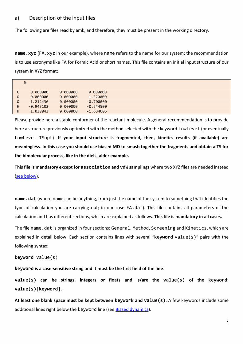
name.xyz (FA.xyz in our example), where name refers to the name for our system; the recommendation

is to use acronyms like FA for Formic Acid or short names. This file contains an initial input structure of our

system in XYZ format:

5 C 0.000000 0.000000 0.000000 O 0.000000 0.000000 1.220000 O 1.212436 0.000000 -0.700000 H -0.943102 0.000000 -0.544500 H 1.038843 0.000000 -1.634005

Please provide here a stable conformer of the reactant molecule. A general recommendation is to provide

here a structure previously optimized with the method selected with the keyword LowLevel (or eventually

LowLevel_TSopt). If your input structure is fragmented, then, kinetics results (if available) are

meaningless. In this case you should use biased MD to smash together the fragments and obtain a TS for

the bimolecular process, like in the diels_alder example.

This file is mandatory except for association and vdW samplings where two XYZ files are needed instead

(see below).

name.dat (where name can be anything, from just the name of the system to something that identifies the

type of calculation you are carrying out; in our case FA.dat). This file contains all parameters of the

calculation and has different sections, which are explained as follows. This file is mandatory in all cases.

The file name.dat is organized in four sections: General, Method, Screening and Kinetics, which are

explained in detail below. Each section contains lines with several “keyword value(s)” pairs with the

following syntax:

keyword value(s)

keyword is a case-sensitive string and it must be the first field of the line.

value(s) can be strings, integers or floats and is/are the value(s) of the keyword:

value(s)[keyword].

At least one blank space must be kept between keywork and value(s). A few keywords include some

additional lines right below the keyword line (see Biased dynamics).

8

Below you will find a detailed explanation of the keywords grouped together in the different sections. For

each section, only the most important keywords are described. Additional keywords can be found in

Advanced options.

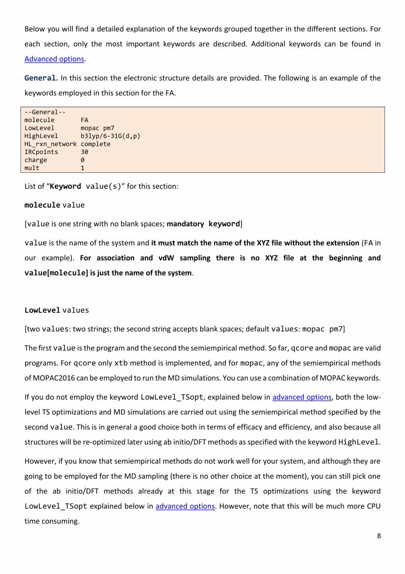
General. In this section the electronic structure details are provided. The following is an example of the

keywords employed in this section for the FA.

--General-- molecule FA LowLevel mopac pm7 HighLevel b3lyp/6-31G(d,p) HL_rxn_network complete IRCpoints 30 charge 0 mult 1

List of “Keyword value(s)” for this section:

molecule value

[value is one string with no blank spaces; mandatory keyword]

value is the name of the system and it must match the name of the XYZ file without the extension (FA in

our example). For association and vdW sampling there is no XYZ file at the beginning and

value[molecule] is just the name of the system.

LowLevel values

[two values: two strings; the second string accepts blank spaces; default values: mopac pm7]

The first value is the program and the second the semiempirical method. So far, qcore and mopac are valid

programs. For qcore only xtb method is implemented, and for mopac, any of the semiempirical methods

of MOPAC2016 can be employed to run the MD simulations. You can use a combination of MOPAC keywords.

If you do not employ the keyword LowLevel_TSopt, explained below in advanced options, both the low-

level TS optimizations and MD simulations are carried out using the semiempirical method specified by the

second value. This is in general a good choice both in terms of efficacy and efficiency, and also because all

structures will be re-optimized later using ab initio/DFT methods as specified with the keyword HighLevel.

However, if you know that semiempirical methods do not work well for your system, and although they are

going to be employed for the MD sampling (there is no other choice at the moment), you can still pick one

of the ab initio/DFT methods already at this stage for the TS optimizations using the keyword

LowLevel_TSopt explained below in advanced options. However, note that this will be much more CPU

time consuming.

9

HighLevel value

[value is one string; no blank spaces; mandatory keyword to run the high-level calculations]

value indicates the level of theory employed in the high-level calculations (using gaussian). You can employ

a dual-level approach, which includes a higher level to refine the energy, as shown in the following example:

HighLevel ccsd(t)/6-311+G(2d,2p)//b3lyp/6-31G(d,p)

Supported methods are HF, MP2 and DFT for geometry optimizations and HF, MP2, DFT and CCSD(T) for

single point energy calculations.

HL_rxn_network value(s)

[one or two values: first is a string, and second (if present) is an integer; default value: reduced]

The first value can be complete or reduced. The value complete indicates that all the TSs will be

reoptimized and in this case no second value is needed.

Alternatively, you may use reduced as the first value (the default), followed by a second value (an

integer) which indicates the maximum energy (in kcal/mol and relative to the reference starting structure)

of a transition state to be calculated at the high level.

IRCpoints value

[value is an integer; default value: 100]

value is the number of IRC points (in each direction) computed at the high-level with gaussian.

charge value

[value is an integer; default value: 0]

value is the charge of the system.

mult value

[value is an integer; default value: 1]

10

value is the multiplicity of the system. Note that this keyword is only employed in the HL calculations. If

you want to run the LL calculations with a specific multiplicity, this should be specified in the LowLevel

keyword using any of the possibilities that MOPAC offers.

Method. Here the user provides details of the method employed for sampling structures. In our FA example,

we have the following:

--Method-- sampling MD ntraj 10

List of “Keyword value(s)” for this section:

sampling value

[value is one string with no blank spaces; default value: MD]

value can be: MD, MD-micro, BXDE, external, ExtForce, association and vdW

MD and MD-micro refer to the type of initial conditions used to run the MD simulations. MD-micro has not

been implemented yet for qcore With BXDE the rare-event acceleration method named BXDE is invoked.3

The BXDE module employs the “Atomistic Simulation Environment” (ASE) library of Python,4 which must be

referenced whenever BXDE is employed.

MD allows the user to include partial constraints in the trajectories, which may be useful for large systems

(see the “advanced users” section for more details).

external allows trajectory data to be read from the results of an external (MD) program. The trajectory

data (in XYZ format) must be stored in a directory named coordir using one file per trajectory which should

be called name_dynX.xyz, where name is value[molecule], and X is the number of each trajectory (X =

1-ntraj). The keyword ntraj must be set accordingly.

ExtForce makes all possible combinations of bond breakages/formations which are consistent with preset

valencies of the atoms and with products lying below the maximum energy of the system. Once the

combinations are known, forces are applied to break/form the selected bonds. This sampling does not need

to include the number of trajectories and has not been implemented yet for qcore.

CAVEAT: To use MD-micro the initial structure needs to be fully optimized and a frequency calculation can

not afford imaginary frequencies. Otherwise choose MD

11

association and vdW are employed to sample van der Waals structures, present some peculiarities and

therefore are explained in detail in van der Waals complexes.

MD, MD-micro, external and BXDE samplings accept the following keywords:

ntraj value

[value is an integer; default value: 1]

value is the number of trajectories. We strongly recommend here to avoid using big numbers of

trajectories. Instead the user should try to run different batches of trajectories as indicated below with a

small number of trajectories each one. One trajectory is recommended for BXDE.

seed value

[value is an integer; only valid for MD and MD-micro; default value: 0]

value is the seed of the random number generator. It can be employed to run a test trajectory. See the

FA_singletraj.dat file in the examples. Only use this keyword for testing.

Screening. Some of the initially located structures might have very low imaginary frequencies, be repeated

or correspond to transition states of van der Waals complexes formed upon fragmentation of the reactant

molecule. To avoid or minimize low-(imaginary)frequency structures, redundancies and van der Waals

complexes, amk includes a screening tool, which is based on the following descriptors: energy, SPRINT

coordinates,5 degrees of each vertex and eigenvalues of the Laplacian matrix.1 While the lowest eigenvalues

of the Laplacian (eigL) are employed to discriminate fragmented structures, comparing the descriptors for

any pair of structures, a mean absolute percentage error (MAPE) and a biggest absolute percentage error

(BAPE) are obtained.

In this section we set a minimum value for the imaginary frequency and maximum values for MAPE, BAPE

and eigL, as explained below:

--Screening -- imagmin 200 MAPEmax 0.008 BAPEmax 2.5 eigLmax 0.1

List of “Keyword value(s)” for this section:

imagmin value

12

[value is an integer; default value: 0]

value is the minimum value for the imaginary frequency (in absolute value and cm−1) of the selected TS

structures.

MAPEmax value

[value is a float; default value: 0]

value is the maximum value for MAPE.

BAPEmax value

[value is a float; default value: 0]

value is the maximum value for BAPE.

If both, the MAPE and BAPE values calculated for two structures are below the values of MAPEmax and

BAPEmax, respectively, the structures are considered equivalent, and therefore only one is kept.

As a general advice, value[MAPEmax] and value[BAPEmax] should be small. A good starting point could

be the values provided in the input files of the examples. Since the HL calculations (performed with G09)

have much more stringent tests for optimization than those of MOPAC, in the screening of the HL structures,

value[MAPEmax] and value[BAPEmax] are set to MIN(MAPEmax, 0.001) and MIN(BAPEmax, 1),

respectively.

eigLmax value

[value is a float; default value: 0]

value is the maximum value for an eigL to be considered 0. In Spectral Graph Theory, the number of zero

eigLs provides the number of fragments in the system. This criterion is used to identify van der Waals

complexes that are formed by unimolecular fragmentation.

Kinetics. This part is employed to provide details for the kinetics calculations at the (experimental)

conditions you want to simulate. This section is compulsory except for association.

An example is given as follows.

--Kinetics-- Energy 150

13

The kinetics simulations will be carried out for a canonical (fixed temperature) or microcanonical (fixed

energy) ensemble, which have their associated keywords:

List of “Keyword value(s)” for this section:

Energy value

[value is an integer; default value: 0]

value is the energy (in kcal/mol) for which microcanonical rate coefficients will be calculated.

Temperature value

[value is an integer; default value: 298]

value is the temperature (in K) for which thermal rate coefficients will be calculated. At present,

temperatures below 100 K are not allowed.

b) Running the dynamics in a single processor

MD and MD-micro methods provide initial coordinates and momenta to run accelerated dynamics

simulations. Select the number of trajectories with ntraj and remember to avoid the seed keyword if the

number of trajectories is greater than 1. In you want to run 10 trajectories, your Method section should look

like (remember that the amk/2020 module must be loaded):

--Method-- sampling MD-micro ntraj 10

The dynamics can be run either in a single processor or in parallel. To run trajectories in a single processor

use the amk.sh script:

amk.sh FA.dat > amk.log &

The ouput file amk.log provides information about the calculations. In addition, a directory called

tsdirLL_FA is created, which contains information that may be useful for checking purposes. We notice

that the program creates a symbolic link to the FA.dat file, named amk.dat, which is used internally by

several amk scripts. At any time, you can check the transition states that have been found using:

tsll_view.sh

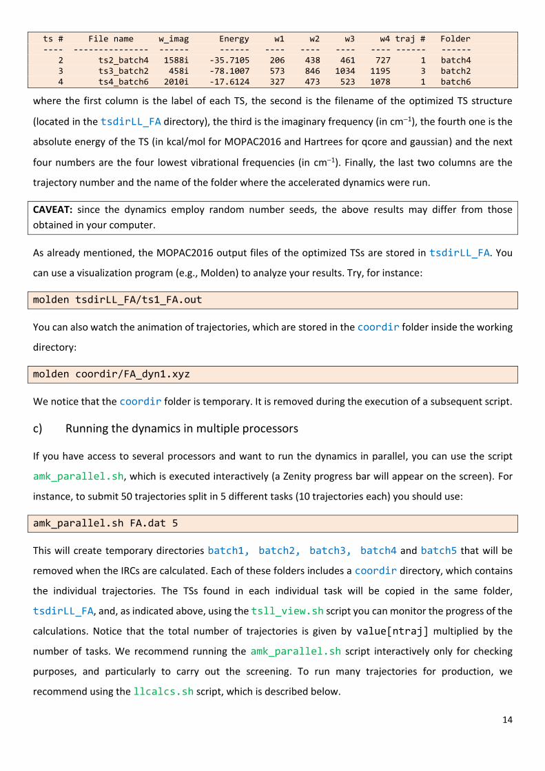
The output of this script will be something like this:

14

ts # File name w_imag Energy w1 w2 w3 w4 traj # Folder ---- --------------- ------ ------ ---- ---- ---- ---- ------ ------ 2 ts2_batch4 1588i -35.7105 206 438 461 727 1 batch4 3 ts3_batch2 458i -78.1007 573 846 1034 1195 3 batch2 4 ts4_batch6 2010i -17.6124 327 473 523 1078 1 batch6

where the first column is the label of each TS, the second is the filename of the optimized TS structure

(located in the tsdirLL_FA directory), the third is the imaginary frequency (in cm−1), the fourth one is the

absolute energy of the TS (in kcal/mol for MOPAC2016 and Hartrees for qcore and gaussian) and the next

four numbers are the four lowest vibrational frequencies (in cm−1). Finally, the last two columns are the

trajectory number and the name of the folder where the accelerated dynamics were run.

CAVEAT: since the dynamics employ random number seeds, the above results may differ from those

obtained in your computer.

As already mentioned, the MOPAC2016 output files of the optimized TSs are stored in tsdirLL_FA. You

can use a visualization program (e.g., Molden) to analyze your results. Try, for instance:

molden tsdirLL_FA/ts1_FA.out

You can also watch the animation of trajectories, which are stored in the coordir folder inside the working

directory:

molden coordir/FA_dyn1.xyz

We notice that the coordir folder is temporary. It is removed during the execution of a subsequent script.

c) Running the dynamics in multiple processors

If you have access to several processors and want to run the dynamics in parallel, you can use the script

amk_parallel.sh, which is executed interactively (a Zenity progress bar will appear on the screen). For

instance, to submit 50 trajectories split in 5 different tasks (10 trajectories each) you should use:

amk_parallel.sh FA.dat 5

This will create temporary directories batch1, batch2, batch3, batch4 and batch5 that will be

removed when the IRCs are calculated. Each of these folders includes a coordir directory, which contains

the individual trajectories. The TSs found in each individual task will be copied in the same folder,

tsdirLL_FA, and, as indicated above, using the tsll_view.sh script you can monitor the progress of the

calculations. Notice that the total number of trajectories is given by value[ntraj] multiplied by the

number of tasks. We recommend running the amk_parallel.sh script interactively only for checking

purposes, and particularly to carry out the screening. To run many trajectories for production, we

recommend using the llcalcs.sh script, which is described below.

15

If the Slurm Workload Manager is installed on your computer, you can submit the jobs to Slurm using:

sbatch [options] amk_parallel.sh FA.dat ntasks

where ntasks is the number of tasks. If no options are specified, sbatch employs the following default

values:

#SBATCH --output=amk_parallel-%j.log

#SBATCH --time=04:00:00

#SBATCH -c 1 --mem-per-cpu=2048

#SBATCH -n 8

These values can be changed when you submit the job with options.

CAVEAT: if you use Slurm Workload Manage for the amk_parallel.sh script, you will have to wait until

all tasks are completed before going on.

d) Analyzing the dynamics results

1) The amk package includes the irc.sh script, which performs intrinsic reaction coordinate

calculations for all the located TSs. This script also allows one to perform an initial screening of the TS

structures before running the IRC calculations:

irc.sh screening

This will do the screening and stop. The process involves the use of tools from Spectral Graph Theory and

utilizes value[MAPEmax], value[BAPEmax] and value[eigLmax]. The redundant and fragmented

structures are printed on screen as well as in the file screening.log which is located in tsdirLL_FA.

MOPAC2016 ouput files are also gathered in tsdirLL_FA, and use filenames initiated by “REPEAT” and

“DISCNT”, which refer to repeated and disconnected (i.e., fragmented) structures, respectively. Please

check these structures and, if needed, change the above parameters. Should you change some of the above

parameters (value[MAPEmax], value[BAPEmax], value[eigLmax]), you need to redo the screening

with the new parameters:

redo_screening.sh

You can repeat the above process until you are happy with the screening.

Once you are confident with the threshold values, you can submit many trajectories to carry out a thorough

exploration of the potential energy surface. Subsequently, you can proceed with the IRC calculations.

2) Obtaining the IRCs:

(sbatch [options]) irc.sh

16

3) Optimizing the minima:

(sbatch [options]) min.sh

4) Creating the reaction network:

rxn_network.sh

Once you have created the reaction network, you can grow your TS list by running more trajectories (with

amk_parallel.sh or amk.sh). Now the trajectories will start from the newly generated minima as well as

from the main structure, specified in the name.xyz file. It is important to notice that, in general, trajectories

run in separate batches (i.e., performed in several tasks) may be initialized from different minima and will

have different energies. In this regard, the efficiency of the code may increase if the calculations are

submitted using a large number for the ntasks parameter.

Convergence in the total number of TSs can be checked doing:

track_view.sh

When you are happy with the obtained TSs or you achieve convergence, you can proceed with the next

steps.

5) Solving the kinetics using KMC with the parameters given in the kinetics section:

kmc.sh

6) Gathering all relevant information in folder FINAL_LL_FA:

final.sh

This folder will gather all the relevant information data, which are described below.

e) Running all low-level calculations using a single script

All the above steps can be done automatically using a single script, called llcalcs.sh. To run this script on

a workstation with the GNU Parallel tool, type

nohup llcalcs.sh name.dat ntasks niter runningtasks >llcalcs.log 2>&1 &

where ntasks is the number of tasks for amk_parallel.sh, niter is the number of amk iterations, and

runningtasks is the number of simultaneous tasks (useful if the workstation is shared by several users).

The script can be run without the arguments (i.e., name.dat, ntasks, niter and runningtasks), and two

pop-up windows will help you enter the arguments.

Finally, if your computer system has the Slurm job scheduler, you can submit the calculations as follows:

17

sbatch llcalcs.sh name.dat ntasks niter

CAVEAT: the use of llcalcs.sh is highly recommended once you have verified that the screening process

works fine for your system.

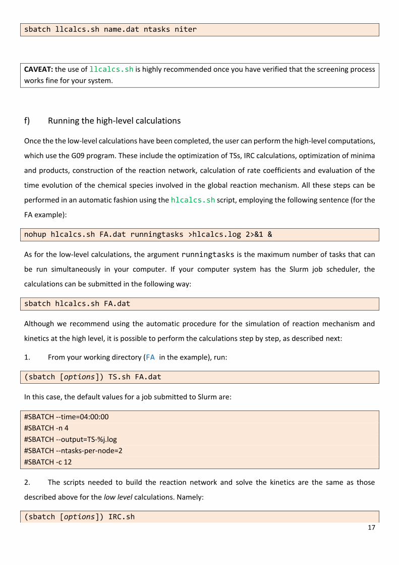
f) Running the high-level calculations

Once the the low-level calculations have been completed, the user can perform the high-level computations,

which use the G09 program. These include the optimization of TSs, IRC calculations, optimization of minima

and products, construction of the reaction network, calculation of rate coefficients and evaluation of the

time evolution of the chemical species involved in the global reaction mechanism. All these steps can be

performed in an automatic fashion using the hlcalcs.sh script, employing the following sentence (for the

FA example):

nohup hlcalcs.sh FA.dat runningtasks >hlcalcs.log 2>&1 &

As for the low-level calculations, the argument runningtasks is the maximum number of tasks that can

be run simultaneously in your computer. If your computer system has the Slurm job scheduler, the

calculations can be submitted in the following way:

sbatch hlcalcs.sh FA.dat

Although we recommend using the automatic procedure for the simulation of reaction mechanism and

kinetics at the high level, it is possible to perform the calculations step by step, as described next:

1. From your working directory (FA in the example), run:

(sbatch [options]) TS.sh FA.dat

In this case, the default values for a job submitted to Slurm are:

#SBATCH --time=04:00:00

#SBATCH -n 4

#SBATCH --output=TS-%j.log

#SBATCH --ntasks-per-node=2

#SBATCH -c 12

2. The scripts needed to build the reaction network and solve the kinetics are the same as those

described above for the low level calculations. Namely:

(sbatch [options]) IRC.sh

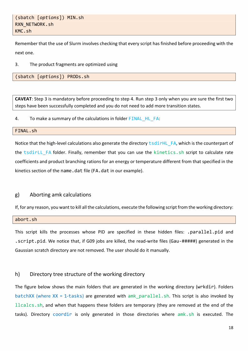
18

(sbatch [options]) MIN.sh

RXN_NETWORK.sh

KMC.sh

Remember that the use of Slurm involves checking that every script has finished before proceeding with the

next one.

3. The product fragments are optimized using

(sbatch [options]) PRODs.sh

CAVEAT: Step 3 is mandatory before proceeding to step 4. Run step 3 only when you are sure the first two

steps have been successfully completed and you do not need to add more transition states.

4. To make a summary of the calculations in folder FINAL_HL_FA:

FINAL.sh

Notice that the high-level calculations also generate the directory tsdirHL_FA, which is the counterpart of

the tsdirLL_FA folder. Finally, remember that you can use the kinetics.sh script to calculate rate

coefficients and product branching rations for an energy or temperature different from that specified in the

kinetics section of the name.dat file (FA.dat in our example).

g) Aborting amk calculations

If, for any reason, you want to kill all the calculations, execute the following script from the working directory:

abort.sh

This script kills the processes whose PID are specified in these hidden files: .parallel.pid and

.script.pid. We notice that, if G09 jobs are killed, the read-write files (Gau-#####) generated in the

Gaussian scratch directory are not removed. The user should do it manually.

h) Directory tree structure of the working directory

The figure below shows the main folders that are generated in the working directory (wrkdir). Folders

batchXX (where XX = 1-tasks) are generated with amk_parallel.sh. This script is also invoked by

llcalcs.sh, and when that happens these folders are temporary (they are removed at the end of the

tasks). Directory coordir is only generated in those directories where amk.sh is executed. The

19

amk_parallel-logs directory contains a series of files that give information on CPU time consumption

for the different calculation steps when they were executed with GNU Parallel. Directories tsdirLL_name

and tsdir_HL_name are generated at runtime and employed to generate the final files and directories. For

that reason, they should not be removed. Finally, the most important files are gathered in directories

FINAL_LL_name and FINAL_HL_name and are described in the next section.

i) Relevant information

As already mentioned, the scripts final.sh and FINAL.sh collect all the relevant information in folders

FINAL_LL_name and FINAL_HL_name, respectively (where name is value[molecule]; in our example

name is FA). These folders contain some files as well as a subdirectory called normal_modes, which includes,

for each structure, a file (in MOLDEN format) with which you can visualize the corresponding normal modes.

The files included in these folders are the following.

convergence.txt lists the number of located transition states as a function of the number of trajectories

and iteration (Only in FINAL_LL_FA).

Energy_profile.pdf is an energy diagram with the relevant paths. If you change the

value[ImpPaths] in the kinetics section of the input data (see below), you will incorporate/remove some

pathways. In our example, the energy diagram is the following:

wrkdir

FINAL_LL_nametsdirHL_name tsdirLL_nameamk_parallel-logsFINAL_HL_name coordir batchXX

normal_modes normal_modes

amk.sh amk_parallel.sh

20

frag_warnings. contains information on failed ab initio calculations of the fragments. If all calculations

are successful, the file is absent. If some of the fragment calculations failed, the file will be located in

FINAL_HL_FA folder.

MINinfo contains information of the minima:

MIN # DE(kcal/mol) 1 -8.341 2 0.000 3 5.288 4 6.732 5 15.441 6 82.122 7 110.400 8 188.254 Conformational isomers are listed in the same line: 1 2 3 4 5

TSinfo contains information of the TSs:

TS # DE(kcal/mol) 1 -1.624 2 1.868 3 9.644 4 25.135 5 32.821 6 37.608 7 40.956 8 44.037 9 53.173 10 58.156 11 60.015 12 85.659 13 142.228 14 188.765 15 191.650 Conformational isomers are listed in the same line:

21

9 11

In the above files, DE is the energy relative to that of the main structure specified in the FA.dat file

(optimized with the semiempirical Hamiltonian). The integers are used to identify, independently, minima

and transition states. Notice that, in this example, MIN 2 corresponds to the structure specified in FA.xyz.

table.db with table being min, prod and ts, which refer to the minima (intermediates), product

fragments and transition states, respectively. These are SQLite3 tables containing the geometries, energies

and frequencies of minima, products and TSs, respectively. The different properties can be obtained using

the select.sh script, which should be run inside the FINAL_LL_FA (or FINAL_HL_FA) folder:

select.sh property table label

where property can be: natom, name, energy, zpe, g, geom, freq, formula (only for prod) or all, and

label is one of the numbers shown in RXNet (see below), which are employed to label each structure. At the

semiempirical level, the energy values correspond to heats of formation. For high-level calculations, the

tables collect the electronic energies. As an example, to obtain the geometry of the first transition state, you

should use:

select.sh geom ts 1

RXNet contains information of the complete reaction network, that is all the elementary reactions found by

the amk program (the file shown below and the following ones were cut and show only up to TS 31).

TS # DE(kcal/mol) Reaction path information ==== ============ ========================= 1 -1.6 PR2: CO + H2O <---> PR2: CO + H2O 2 1.9 MIN 1 <---> MIN 2 3 9.6 MIN 3 <---> MIN 4 4 25.1 MIN 1 <---> MIN 1 5 32.8 PR2: CO + H2O <---> PR1: H2 + CO2 6 37.6 MIN 4 ----> PR2: CO + H2O 7 41.0 MIN 1 ----> PR2: CO + H2O 8 44.0 PR1: H2 + CO2 <---> PR1: H2 + CO2 9 53.2 MIN 1 <---> MIN 4 10 58.2 MIN 2 ----> PR1: H2 + CO2 11 60.0 MIN 2 <---> MIN 5 12 85.7 MIN 2 <---> MIN 6 13 142.2 MIN 3 <---> MIN 6 14 188.8 MIN 2 <---> MIN 8 15 191.7 MIN 7 <---> MIN 8

As can be seen, for each transition state, this file specifies the associated minima and/or product fragments

and their corresponding identification numbers. Notice that TS, MIN and PR have independent identification

numbers. If you use the option complete for the keyword HL_rxn_network (in the General section of

the input data), all the TSs will be reoptimized in the high-level calculations. You may reduce significantly the

number of TSs to be reoptimized in the HL calculations, and therefore the reaction network, if you use the

22

option reduced. If it is employed without an argument, TSs associated to PR <--> PR steps (i.e.,

bimolecular reactions) and to interconversion between optical isomers will not be reoptimized in the HL

calculations. You may include a number as an argument of this option:

HL_rxn_network reduced 55

In this case, besides the above TSs, all TSs having relative energies larger than 55 kcal/mol will not be

considered for HL optimizations, that is, they will not be included in the HL reaction network. We notice that

the last argument must be an integer.

RXNet.cg. By default (see below) the KMC calculations are “coarse-grained”, that is, conformational

isomers form a single state, which is taken as the lowest energy isomer. Such reaction network, which also

removes bimolecular channels, is the following:

TS # DE(kcal/mol) Reaction path information ==== ============ ========================= 6 37.6 MIN 3 ----> PR2: CO + H2O CONN 7 41.0 MIN 1 ----> PR2: CO + H2O CONN 9 53.2 MIN 1 <---> MIN 3 CONN 10 58.2 MIN 1 ----> PR1: H2 + CO2 CONN 11 60.0 MIN 1 <---> MIN 3 CONN 12 85.7 MIN 1 <---> MIN 6 CONN 13 142.2 MIN 3 <---> MIN 6 CONN 14 188.8 MIN 1 <---> MIN 8 DISCONN 15 191.7 MIN 7 <---> MIN 8 DISCONN

The last column with the flag “CONN” or “DISCONN” indicates whether the given process is connected with

the others (CONN) or whether it is isolated (DISCONN). This flag is useful when you choose a starting

intermediate for the KMC simulations, because that intermediate should be connected with the others. If

you want to include all conformational isomers explicitly in the KMC simulations, you need to construct the

reaction network by using the allstates option, as described in the next section.

RXNet.rel is similar to RXNet.cg, but only collects the relevant paths, that is, those included in the

Energy_profile.pdf file.

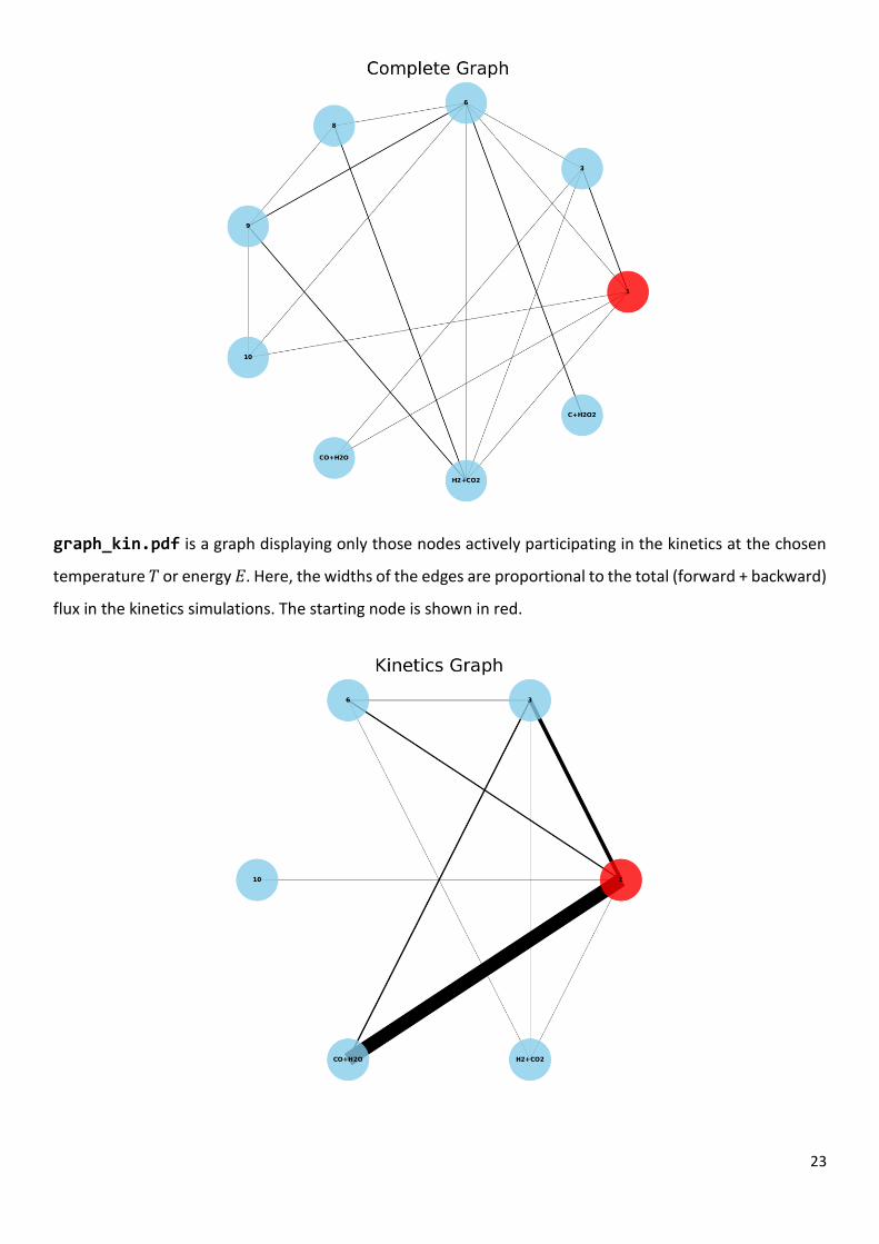
graph_all.pdf is a graph displaying RXNet.cg reaction network. The nodes correspond to reactant,

intermediates and products, and the widths of the edges are proportional to the number of paths connecting

the corresponding nodes. The starting node is shown in red.

23

graph_kin.pdf is a graph displaying only those nodes actively participating in the kinetics at the chosen

temperature 𝑇 or energy 𝐸. Here, the widths of the edges are proportional to the total (forward + backward)

flux in the kinetics simulations. The starting node is shown in red.

24

rxn_x.txt (x = all, kin, stats) are files with information relevant for the reaction network analysis

made with NetworkX python library.6 Each line of rxn_all.txt lists the nodes (first two columns) and the

weight (last column), which is the number of paths connecting the two nodes. For rxn_kin.txt the weight

is the total flux in the kinetics simulations. These two files are employed to construct graph_all.pdf and

graph_kin.pdf, respectively. In rxn_stats.txt, some properties of the reaction network are listed, like

the average shortest path length, the average clustering coefficient, the transitivity, etc. The user is

encouraged to read the NetworkX documentation and ref 7.

kineticsFvalue contains the kinetics results, namely, the final branching ratios and the population of

every species as a function of time. In the name of the file, F is either “T” or “E” for temperature or energy,

and “value” is the corresponding value. For instance, the kinetics results for a canonical calculation at 298

K would be printed in a file called kineticsT298. A file called populationFvalue.pdf is also available.

It is a plot with the population of each species as a function of time. The following figure shows an example

of such a plot obtained for the decomposition of FA using the PM7 stationary points.

j) Details of the kinetics simulations

Except for vdW sampling, for the KMC simulations the different conformational isomers form a single state,

which speeds up the calculations. If you prefer to treat each conformational isomer as a single state, you

should run the rxn_network.sh script again (or RXN_NETWORK.sh for the high level), using the argument

25

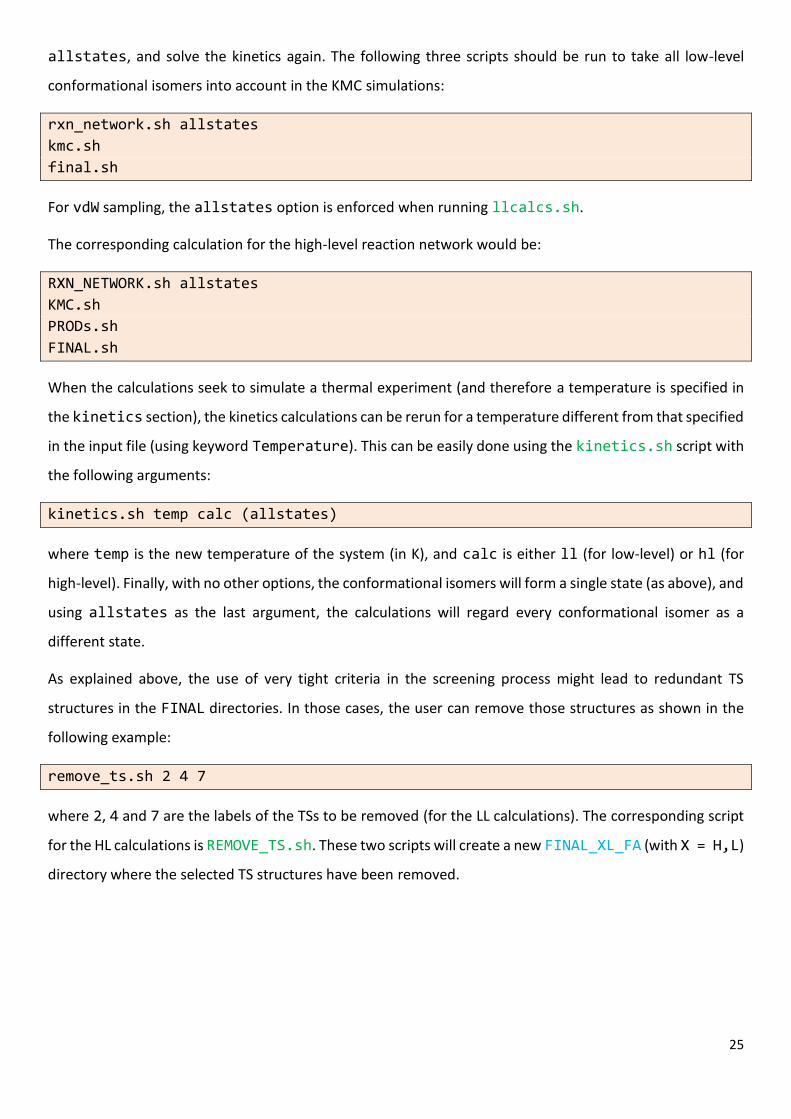
allstates, and solve the kinetics again. The following three scripts should be run to take all low-level

conformational isomers into account in the KMC simulations:

rxn_network.sh allstates

kmc.sh

final.sh

For vdW sampling, the allstates option is enforced when running llcalcs.sh.

The corresponding calculation for the high-level reaction network would be:

RXN_NETWORK.sh allstates

KMC.sh

PRODs.sh

FINAL.sh

When the calculations seek to simulate a thermal experiment (and therefore a temperature is specified in

the kinetics section), the kinetics calculations can be rerun for a temperature different from that specified

in the input file (using keyword Temperature). This can be easily done using the kinetics.sh script with

the following arguments:

kinetics.sh temp calc (allstates)

where temp is the new temperature of the system (in K), and calc is either ll (for low-level) or hl (for

high-level). Finally, with no other options, the conformational isomers will form a single state (as above), and

using allstates as the last argument, the calculations will regard every conformational isomer as a

different state.

As explained above, the use of very tight criteria in the screening process might lead to redundant TS

structures in the FINAL directories. In those cases, the user can remove those structures as shown in the

following example:

remove_ts.sh 2 4 7

where 2, 4 and 7 are the labels of the TSs to be removed (for the LL calculations). The corresponding script

for the HL calculations is REMOVE_TS.sh. These two scripts will create a new FINAL_XL_FA (with X = H,L)

directory where the selected TS structures have been removed.

26

6. Other capabilities

a) van der Waals complexes

AutoMeKin includes an option to predict van der Waals (vdW) complexes. In principle two related sampling

options are available: association and vdW. While association runs a number of structure

optimizations for randomly rotated fragments, vdW is a more powerful option representing a natural

extension of our bbfs method to study vdW complexes.8 The input files for these two options slightly differ

from those explained previously, as detailed below.

association. Here, a number of full optimizations are performed starting from random orientations of A

and B. An example of such input file can be found in path_to_program/examples/assoc.dat. Two

additional input files are also needed for this example, Bz.xyz and N2.xyz, which are also available in the

same folder. The assoc.dat file contains the following data:

--General-- molecule Bz-N2 fragmentA Bz fragmentB N2 --Method-- sampling association rotate com com 4.0 1.5 Nassoc 50 --Screening-- MAPEmax 0.0001 BAPEmax 0.5 eigLmax 0.05

This type of sampling only needs three sections: General, Method and Screening. Some further keyword

value(s) pairs are needed for this sampling:

fragmentA value

[value is one string with no blank spaces; mandatory keyword]

value is the name of fragment A (Bz in our case). A file with the Cartesian coordinates Bz.xyz must be

present in the working directory.

fragmentB value

[value is one string with no blank spaces; mandatory keyword]

27

value is the name of fragment B (N2 in our case). A file with the Cartesian coordinates N2.xyz must be

present as well.

rotate values

[four values: first two can be strings or integers and last two are floats; default values: com com 4.0

1.5]

The first two values are the pivot positions of the random rotations: the center of mass (com) of fragment

A and the center of mass of fragment B in our example (these pivots could be labels of atoms and therefore

integers). The last two values are the distance (in Å) between both pivots and the minimum intermolecular

distance between any two atoms of both fragments, respectively.

Nassoc value

[value is an integer; default value: 100]

value is the total number of intermolecular structures considered in the sampling. With this sampling, you

cannot perform kinetics. However, you still need to provide the parameters for the screening. To run the

calculations, just type:

amk.sh assoc.dat

This job will submit Nassoc independent optimizations to find the structures. After the jobs finished, the

script will automatically remove duplicates and select the best association “complex”.

Note that you cannot use amk_parallel.sh with this option, as this script is only employed to run MD

simulations.

You can check the optimized structures in folder assoc_Bz_N2. The program will also select the “best”

structure according to the minimum number of structural changes between the complex and the individual

fragments and its energy. The structure selected will be called Bz-N2.xyz. For fragments containing metals,

the selection is also based on the valence of the metal center. The file assoclist_sorted (in the

assoc_Bz_N2 folder) collects a summary of the structures and their energies, as well as the MOPAC2016

output files of each of them, which are called assocN.out, where N is a number from 1 to Nassoc.

vdW. For this option, the first part is common to association, and the program runs Nassoc independent

optimizations to get an initial structure of the complex. From that point onwards, the program performs

28

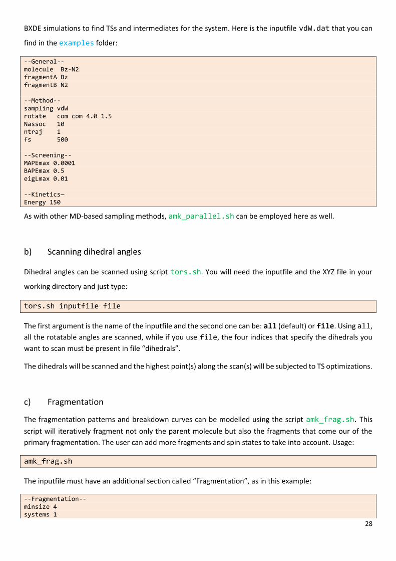
BXDE simulations to find TSs and intermediates for the system. Here is the inputfile vdW.dat that you can

find in the examples folder:

--General-- molecule Bz-N2 fragmentA Bz fragmentB N2 --Method-- sampling vdW rotate com com 4.0 1.5 Nassoc 10 ntraj 1 fs 500 --Screening-- MAPEmax 0.0001 BAPEmax 0.5 eigLmax 0.01

--Kinetics— Energy 150

As with other MD-based sampling methods, amk_parallel.sh can be employed here as well.

b) Scanning dihedral angles

Dihedral angles can be scanned using script tors.sh. You will need the inputfile and the XYZ file in your

working directory and just type:

tors.sh inputfile file

The first argument is the name of the inputfile and the second one can be: all (default) or file. Using all,

all the rotatable angles are scanned, while if you use file, the four indices that specify the dihedrals you

want to scan must be present in file “dihedrals”.

The dihedrals will be scanned and the highest point(s) along the scan(s) will be subjected to TS optimizations.

c) Fragmentation

The fragmentation patterns and breakdown curves can be modelled using the script amk_frag.sh. This

script will iteratively fragment not only the parent molecule but also the fragments that come our of the

primary fragmentation. The user can add more fragments and spin states to take into account. Usage:

amk_frag.sh

The inputfile must have an additional section called “Fragmentation”, as in this example:

--Fragmentation-- minsize 4 systems 1

29

CH3O+ 3

The new keywords are explained below.

minsize value

[value is an integer; default value: 4]

value is the minimum number of atoms for a fragment to be considered in secondary fragmentations.

systems ns

sys(1) mult(1)

sys(2) mult(2)

…

sys(ns) mult(ns)

ns is the number of additional fragments (or systems) to be considered in secondary fragmentations (default

value: 0), besides those obtained in the fragmentation of the parent molecule. These could be fragments

with other spin state, or fragments that are obtained through a barrierless process. This line must be

followed by ns lines with two columns each one: the formula of each system (sys) and its multiplicity

(mult). Note that for the formula the chemical symbols of the atoms must sorted following AutoMeKin’s

convention: alphabetic order.

In the example above, only fragments with number of atoms greater than or equal to 4 are further

fragmented and an additional system has been added: CH3O+ in its triplet state.

This workflow creates a new folder: M3Cinp containing files that can be read by program M3C to simulate

the breakdown curves of the studied molecule.

d) Advanced options

The following are keywords that can be useful for experienced users.

General

iop value

[value is one string with no blank spaces; no default value]

value is a gaussian IOp string. Example:

30

HighLevel mpwb95/6-31+G(d,p)

iop iop(3/76=0560004400)

LowLevel_TSopt values

[two values: two strings; no blank spaces in each string; default values: mopac value[LowLevel]]

First value is the program and second value is the electronic structure level employed to optimize the TSs

at the low-level stage. This keyword is employed if you want to use gaussian (which is the only ab initio

program interfaced with amk) for the low-level TS optimizations, as shown in the example below but take

into account that it is very CPU-time consuming. Besides the TSs, the starting minimum in name.xyz is also

optimized at this level of theory.

LowLevel_TSopt gaussian hf/3-21g

Method

atoms value(s)

[one or two values: first is a string with no blank spaces or an integer and second (if present) is a string

with no blank spaces; only with MD; default value: all]

The first value can be all (in which case no other values are needed) or the number of atoms initially

excited followed by a second value (string), which is the list of atoms separated by commas (without blank

spaces). It is analogous to modes (explained below). This is an example where atoms 1, 2 and 3 are initially

excited.

atoms 3 1,2,3

etraj value

[value is an integer or string with no blank spaces; only with MD-micro; no default]

If an integer, value is the energy (in kcal/mol) of the MD-micro simulations. If value is a range as in the

example below, the energy is randomly selected in the given energy range.

etraj 200-300

If etraj is not specified, the program automatically employs the following range of energies: [16.25 × (𝑠 −

1) − 46.25 × (𝑠 − 1)] kcal/mol, where s is the number of vibrational degrees of freedom of the system. The

31

values 16.25 and 46.25 have been determined from the formic acid results and making use of RRK theory.

The program automatically adjusts the range to obtain at least 60% reactivity at the boundaries.

factorflipv value

[value is a float; only with MD and MD-micro; no default]

Using the default options, trajectories are halted when the simulation time reaches the value[fs] keyword

(see below) or when there an interatomic distance, 𝑟𝑖𝑗, reaches 5 times its initial value 𝑟𝑖𝑗0, which is regarded

as a fragmentation. Using factorflipv fragmentation can be prevented because the atomic velocities

change their sign:

�⃗�𝑘 = {−�⃗�𝑘 if 𝑘 = 𝑖 or 𝑗

−0.9 × �⃗�𝑘 if 𝑘 ≠ 𝑖 or 𝑗

whenever the following relationship is fulfilled:

𝑟𝑖𝑗 ≥ FP × 𝑟𝑖𝑗0

where FP is value[factorflipv]. We recommend this value to be in the range 3.0-5.0.

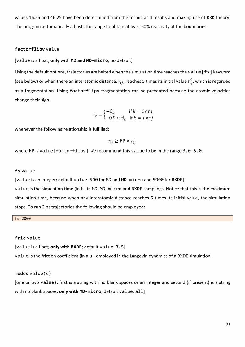
fs value

[value is an integer; default value: 500 for MD and MD-micro and 5000 for BXDE]

value is the simulation time (in fs) in MD, MD-micro and BXDE samplings. Notice that this is the maximum

simulation time, because when any interatomic distance reaches 5 times its initial value, the simulation

stops. To run 2 ps trajectories the following should be employed:

fs 2000

fric value

[value is a float; only with BXDE; default value: 0.5]

value is the friction coefficient (in a.u.) employed in the Langevin dynamics of a BXDE simulation.

modes value(s)

[one or two values: first is a string with no blank spaces or an integer and second (if present) is a string

with no blank spaces; only with MD-micro; default value: all]

32

The first value can be all (in which case no other values are needed) or the number of modes initially

excited followed by a second value (string), which is the list of modes separated by commas (without blank

spaces). It is analogous to atoms (explained above).

multiple_minima value

[value is one string: yes or no; default value: yes]

value can be yes, in which case the exploratory simulations start from multiple minima, or no, where the

all the MD simulations start from the input initial structure.

nforces value

[value is one integer; only with ExtForce; default value: 4]

value is the number of different forces applied to form the bonds in ExtForce sampling. Preliminary tests

show that the results are most sensitive to the value chosen for this force and that is why several forces are

tested.

post_proc value(s)

[from one to three values: first value is a string (bbfs, bots or no), the second and third are integers or

floats; default values: bbfs 20 1 for all samplings except association where the only default value

is no]

The first value is the post-processing algorithm employed to detect reaction events and it can be bbfs (the

default), bots9 or no (if no algorithm is applied; this makes only sense for the purpose of testing the MD

module). For bbfs two more values can follow: the time window (in fs) employed by bbfs and the number

of guess structures selected per candidate. Possible choices for this last number can be 1 or 3. Example:

post_proc bbfs 20 1

If bots (for bond order time series) is employed (only with BXDE, vdW and external), the algorithm

developed by Hutchings et al. is employed,9 which is based on peak finding on the first time derivative of the

bond orders. In this case the two additional values are the cutoff frequency (in cm−1) for the low-pass filter

used to smooth bond order time series, and the number of standard deviations considered to identify peaks

associated with reactive events. The default values for this algorithm are:

post_proc bots 200 2.5

33

temp value

[value is an integer or string with no blank spaces; only with MD and BXDE; no default]

If an integer, value is the temperature (in K) of the MD or BXDE simulations. If a range (only valid for MD),

the temperature is randomly selected in the given range. In the absence of the temp keyword, the program

automatically defines the following range of temperatures: [5452.04 × (𝑠 − 1)/𝑛𝑎𝑡𝑜𝑚 − 15517.34 × (𝑠 −

1)/𝑛𝑎𝑡𝑜𝑚] K, which has been optimized for formic acid. However, as for etraj, the boundaries are adjusted

“on the fly” to obtain a minimum reactivity of 60%. For BXDE, temp has only one value (with 1000 being

the default).

thmass value

[value is an integer; only with MD; default value: 0]

value is the required minimum mass (in a.u.) of an atom to be initially excited.

Kinetics

imin value

[value is an integer or one string: min0; default value: min0]

value is the starting minimum for the KMC simulations. value can be an integer, which identifies the

desired structure or min0, which refers to the input structure. All the minima are listed in MINinfo file and

the user must examine RXNet.cg file to check that the minimum is indeed connected with the other ones

(last column of each pathway indicates this fact).

nmol value

[value is an integer; default value: 1000]

value is the number of molecules for the KMC simulations.

Stepsize value

[value is an integer; default value: 10]

value is the number of reactions that have to take place before printing the population in the KMC runs.

34

MaxEn value

[value is an integer; default value: 100 for thermal kinetics or 3/2 the value of Energy for

microcanonical kinetics]

value is the maximum allowed energy (in kcal/mol and relative to the input structure) for a TS to be included

in the reaction network.

ImpPaths value

[value is a float; default value: 0.1]

value is the minimum percentage of processes occurring through a particular pathway (in the KMC

simulation) that has to be achieved in order to be considered relevant and finally included in the

Energy_profile.pdf file. If value[ImpPaths] is 0.1, it means that pathways contributing less than

0.1% to product formation are not included in this file. If you want to include them all use 0. Notice that

these pathways may refer to the “coarse-grained” mechanism (default option) or to the complete

mechanism that includes conformational isomers (obtained by using the allstates option as described

above).

e) Biased dynamics

AutoMeKin includes several methods to bias the dynamics towards specific reaction pathways. So far, these

are the available options (only for MD and MD-micro):

1) The first option uses the AXD algorithm described in Ref 10, with which selected bond lengths are not

allowed to stretch more than 30% with respect to their initial values. This can be useful to prevent the

breakage of certain bonds. This option can be used invoked using the following keyword nfr pair:

nbondsfrozen nfr

fr_i(1) fr_j(1)

fr_i(2) fr_j(2)

…

fr_i(nfr) fr_j(nfr)

[nfr, fr_i(1,…,nfr) and fr_j(1,…,nfr) are integers; default nfr: 0]

35

where nfr is the number of constrained bonds. The line containing this keyword nfr pair must be followed

by nfr lines, each one with two values (fr_i(1,…,nfr) and fr_j(1,…,nfr), which are integers)

indicating the indexes (labels) of the atoms that form each constrained bond, as in the following example

nbondsfrozen 2 1 13 2 8

This would “freeze” two bond distances connecting atoms 1 and 13 and 2 and 8, respectively.

2) The second algorithm bias the dynamics towards a particular reaction channel. An example of this

option is provided in file path_to_program/examples/FA_biasH2.dat (you also need FA.xyz), which

illustrates a way to search for H2 elimination transition states from formic acid. For this we use two sets of

keywords to apply constant external forces to break or form bonds. For bond breakage we use the following:

nbondsbreak nbr

br_i(1) br_j(1) force(1)

br_i(2) br_j(2) force(2)

…

br_i(nbr) br_j(nbr) force(nbr)

[nbr, br_i(1,…,nbr) and br_j(1,…,nbr) are integers and force(1,…,nbr) are floats; default nbr:

0]

where nbr is the number of bonds we want to break. The line containing this keyword nbr pair must be

followed by nbr lines, each one with three values (br_i(1,…,nbr), br_j(1,…,nbr) and

force(1,…,nbr), of which the first two are integers and the last a float). These three numbers indicate

the indexes (labels) of the atoms that form each bond we want to break, and the magnitude of the applied

external force (in kcal/mol/Å), respectively.

For bond formation we use the analogous keyword nbondsform as in this example (taken from

FA_biasH2.dat):

nbondsform 1 4 5 30 nbondsbreak 2 3 5 80 1 4 80

A similar test can be performed on the same molecule to get the TS for H2O elimination. The corresponding

input file, FA_biasH2O.dat, is also available in directory path_to_program/examples. Additionally, a

36

retro Diels-Alder reaction has also been tested (cyclohexene → ethylene+1,3-butadiene), using the input

files rdiels_bias.dat and rdiels.xyz provided in the amk distribution.

The above examples can be tested using the amk.sh script:

amk.sh inputfile

37

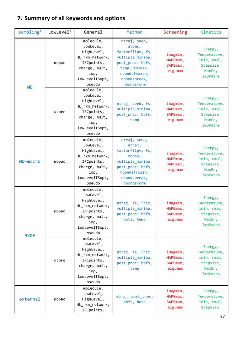
7. Summary of all keywords and options

sampling1 LowLevel2 General Method Screening Kinetics

MD

mopac

molecule,

LowLevel,

HighLevel,

HL_rxn_network,

IRCpoints,

charge, mult,

iop,

LowLevelTSopt,

pseudo

ntraj, seed,

atoms,

factorflipv, fs,

multiple_minima,

post_proc: bbfs,

temp, thmass,

nbondsfrozen,

nbondsbreak,

nbondsform

imagmin,

MAPEmax,

BAPEmax,

eigLmax

Energy,

Temperature,

imin, nmol,

Stepsize,

MaxEn,

ImpPaths

qcore

molecule,

LowLevel,

HighLevel,

HL_rxn_network,

IRCpoints,

charge, mult,

iop,

LowLevelTSopt,

pseudo

ntraj, seed, fs,

multiple_minima,

post_proc: bbfs,

temp

imagmin,

MAPEmax,

BAPEmax,

eigLmax

Energy,

Temperature,

imin, nmol,

Stepsize,

MaxEn,

ImpPaths

MD-micro mopac

molecule,

LowLevel,

HighLevel,

HL_rxn_network,

IRCpoints,

charge, mult,

iop,

LowLevelTSopt,

pseudo

ntraj, seed,

etraj,

factorflipv, fs,

modes,

multiple_minima,

post_proc: bbfs,

nbondsfrozen,

nbondsbreak,

nbondsform

imagmin,

MAPEmax,

BAPEmax,

eigLmax

Energy,

Temperature,

imin, nmol,

Stepsize,

MaxEn,

ImpPaths

BXDE

mopac

molecule,

LowLevel,

HighLevel,

HL_rxn_network,

IRCpoints,

charge, mult,

iop,

LowLevelTSopt,

pseudo

ntraj, fs, fric,

multiple_minima,

post_proc: bbfs,

bots, temp

imagmin,

MAPEmax,

BAPEmax,

eigLmax

Energy,

Temperature,

imin, nmol,

Stepsize,

MaxEn,

ImpPaths

qcore

molecule,

LowLevel,

HighLevel,

HL_rxn_network,

IRCpoints,

charge, mult,

iop,

LowLevelTSopt,

pseudo

ntraj, fs, fric,

multiple_minima,

post_proc: bbfs,

temp

imagmin,

MAPEmax,

BAPEmax,

eigLmax

Energy,

Temperature,

imin, nmol,

Stepsize,

MaxEn,

ImpPaths

external mopac

molecule,

LowLevel,

HighLevel,

HL_rxn_network,

IRCpoints,

ntraj, post_proc:

bbfs, bots

imagmin,

MAPEmax,

BAPEmax,

eigLmax

Energy,

Temperature,

imin, nmol,

Stepsize,

38

charge, mult,

iop,

LowLevelTSopt,

pseudo

MaxEn,

ImpPaths

qcore

molecule,

LowLevel,

HighLevel,

HL_rxn_network,

IRCpoints,

charge, mult,

iop,

LowLevelTSopt,

pseudo

ntraj, post_proc:

bbfs

imagmin,

MAPEmax,

BAPEmax,

eigLmax

Energy,

Temperature,

imin, nmol,

Stepsize,

MaxEn,

ImpPaths

ExtForce mopac

molecule,

LowLevel,

HighLevel,

HL_rxn_network,

IRCpoints,

charge, mult,

iop,

LowLevelTSopt,

pseudo

nforces

imagmin,

MAPEmax,

BAPEmax,

eigLmax

Energy,

Temperature,

imin, nmol,

Stepsize,

MaxEn,

ImpPaths

associati

on

mopac

molecule,

fragmentA,

fragmentB,

LowLevel

rotate, Nassoc

MAPEmax,

BAPEmax,

eigLmax

qcore

molecule,

fragmentA,

fragmentB,

LowLevel

rotate, Nassoc

MAPEmax,

BAPEmax,

eigLmax

vdW

mopac

molecule,

fragmentA,

fragmentB,

LowLevel,

HighLevel,

IRCpoints, iop,

LowLevelTSopt,

pseudo

rotate, Nassoc,

ntraj, fs, fric,

multiple_minima,

post_proc: bbfs

imagmin,

MAPEmax,

BAPEmax,

eigLmax

Energy,

Temperature,

imin, nmol,

Stepsize,

MaxEn,

ImpPaths

qcore

molecule,

fragmentA,

fragmentB,

LowLevel,

HighLevel,

IRCpoint, iop,

LowLevelTSopt,

pseudo

rotate, Nassoc,

ntraj, fs, fric,

multiple_minima,

post_proc: bbfs

imagmin,

MAPEmax,

BAPEmax,

eigLmax

Energy,

Temperature,

imin, nmol,

Stepsize,

MaxEn,

ImpPaths

1Value of sampling keyword (in section: Method). 2First value of LowLevel keyword, i.e., program, (in section

General).

39

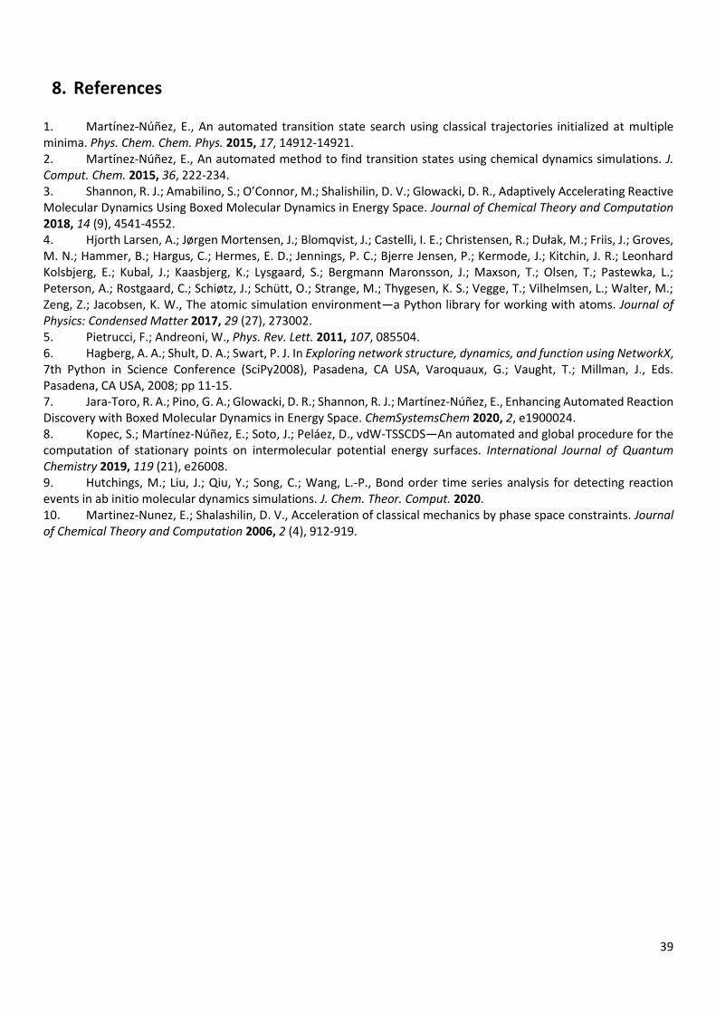
8. References

1. Martínez-Núñez, E., An automated transition state search using classical trajectories initialized at multiple minima. Phys. Chem. Chem. Phys. 2015, 17, 14912-14921. 2. Martínez-Núñez, E., An automated method to find transition states using chemical dynamics simulations. J. Comput. Chem. 2015, 36, 222-234. 3. Shannon, R. J.; Amabilino, S.; O’Connor, M.; Shalishilin, D. V.; Glowacki, D. R., Adaptively Accelerating Reactive Molecular Dynamics Using Boxed Molecular Dynamics in Energy Space. Journal of Chemical Theory and Computation 2018, 14 (9), 4541-4552. 4. Hjorth Larsen, A.; Jørgen Mortensen, J.; Blomqvist, J.; Castelli, I. E.; Christensen, R.; Dułak, M.; Friis, J.; Groves, M. N.; Hammer, B.; Hargus, C.; Hermes, E. D.; Jennings, P. C.; Bjerre Jensen, P.; Kermode, J.; Kitchin, J. R.; Leonhard Kolsbjerg, E.; Kubal, J.; Kaasbjerg, K.; Lysgaard, S.; Bergmann Maronsson, J.; Maxson, T.; Olsen, T.; Pastewka, L.; Peterson, A.; Rostgaard, C.; Schiøtz, J.; Schütt, O.; Strange, M.; Thygesen, K. S.; Vegge, T.; Vilhelmsen, L.; Walter, M.; Zeng, Z.; Jacobsen, K. W., The atomic simulation environment—a Python library for working with atoms. Journal of Physics: Condensed Matter 2017, 29 (27), 273002. 5. Pietrucci, F.; Andreoni, W., Phys. Rev. Lett. 2011, 107, 085504. 6. Hagberg, A. A.; Shult, D. A.; Swart, P. J. In Exploring network structure, dynamics, and function using NetworkX, 7th Python in Science Conference (SciPy2008), Pasadena, CA USA, Varoquaux, G.; Vaught, T.; Millman, J., Eds. Pasadena, CA USA, 2008; pp 11-15. 7. Jara-Toro, R. A.; Pino, G. A.; Glowacki, D. R.; Shannon, R. J.; Martínez-Núñez, E., Enhancing Automated Reaction Discovery with Boxed Molecular Dynamics in Energy Space. ChemSystemsChem 2020, 2, e1900024. 8. Kopec, S.; Martínez-Núñez, E.; Soto, J.; Peláez, D., vdW-TSSCDS—An automated and global procedure for the computation of stationary points on intermolecular potential energy surfaces. International Journal of Quantum Chemistry 2019, 119 (21), e26008. 9. Hutchings, M.; Liu, J.; Qiu, Y.; Song, C.; Wang, L.-P., Bond order time series analysis for detecting reaction events in ab initio molecular dynamics simulations. J. Chem. Theor. Comput. 2020. 10. Martinez-Nunez, E.; Shalashilin, D. V., Acceleration of classical mechanics by phase space constraints. Journal of Chemical Theory and Computation 2006, 2 (4), 912-919.