Autocalls versus underlying assets

BACHELOR THESIS WITHIN: Economics NUMBER OF CREDITS: 15 hp PROGRAMME OF STUDY: International Economics AUTHOR: Elias Wårhag & Ioan Tepes JÖNKÖPINGMay 2020

A study on how changes in the return of the underlying assets affect the autocall’s returns

i

Acknowledgment We would like to take this opportunity and acknowledge the support from our tutor, Michael Ols-

son, who has guided us and offered valuable input throughout the writing of this thesis.

We would also like to thank the members of our seminar group who have read numerous drafts

and given their views on the strength and weaknesses in the thesis.

Finally, a big thanks to our families who have supported and encouraged us during our time at

Jönköping International Business School.

_________________________ _________________________

Elias Wårhag Ioan Tepes

ii

Bachelor Thesis in Economics Title: Autocalls versus underlying assets: A study on how changes in the return of the un-derlying assets affect the autocalls returns Authors: Wårhag, Elias and Tepes, Ioan Tutor: Michael Olsson Date: 2020-05-18 Key terms: Autocallable structued products, Structured notes, Structured products, Express certif-icate Abstract

Autocallable structured products represent an investment opportunity which has been growing in

both the European and American market since they were first launched. The value of these struc-

tured products is dependent on how their underlying assets perform, which can consist of stocks,

indexes or other assets. With a sample size of 30 structured products we provide research on the

relation between the products return and the return of the underlying assets. Specifically, the pur-

pose of the study is to analyse how increases in the returns of the underlying assets affect the

returns in the products. Using an ordinary least squares regression model, we find that the return

in the underlying assets, the issuers credit rating and the interest rate at issuance have a statistically

significant effect on the returns in the products. We conclude that in our sample, an increase in the

underlying assets returns results in a less than equal increase in the returns of the autocalls.

iii

Table of Contents 1. Introduction ......................................................................... 12. Theory .................................................................................. 32.1 Autocallable Structured Products ........................................................... 32.2 Creation Process of Structured Products ............................................... 62.3 Valuation Process of Autocallable Structured Products ......................... 82.4 Risks in an Autocall ................................................................................ 92.5 Valuation of Stocks ............................................................................... 102.6 Hypothesis ............................................................................................ 12

3. Data .................................................................................... 133.1 Dependent variable ............................................................................... 133.2 Independent variables .......................................................................... 14

4. Method ............................................................................... 174.1 Quantitative research ............................................................................ 174.2 Methodology ......................................................................................... 174.3 Descriptive statistics ............................................................................. 184.4 Correlation matrix ................................................................................. 194.5 VIF ........................................................................................................ 19

5. Result ................................................................................. 216. Analysis ............................................................................. 236.1 Limitations ............................................................................................. 25

7. Conclusion ........................................................................ 26Reference list ................................................................................ 27Appendix ........................................................................................ 31

1

1. Introduction

Autocallable structured products, kick-out plans, structured notes and express certificates,

these are all names of the same product that has attracted great interest from investors since

its first issuance in the early 1990s. In Germany alone, the market volume more than tripled

from EUR 5.25 billion in June 2012 to EUR 17.91 billion in June 2019 (Deutscher Derivate

Verband, 2019). In Sweden, the number of exchange listed products nearly doubled from

8,800 in to 2014 to 16,700 in 2019 and a similar trend can be seen across the European

market (EUSIPA, 2019). By 2014, structured products made up around three percent of

Swedish household's assets (Finansinspektionen, 2014).

In 2019, Sweden’s Financial Regulatory Authority conducted a study that showed the median

commission for a structured products broker was 3.5 percent, ranging as high as up to 30

percent. To put it in perspective, the median commission for a broker of a mutual fund was

0.45 percent (Finansinspektionen, 2019). Per H Börjesson, the founder of Spiltan Fonder,

expresses his discontent with structured products and criticizes hard selling brokers who

persuade retail investors to sell conventional funds to invest in these products. He is sup-

ported by Claes Hemberg who questions why the law of financial advisory does not stop

sales of this kind of products (Mellqvist, 2017).

Apart from the fee, these products are not always traded openly in a market which can lead

to low second-hand value for the products if the investor must sell before the expiration

date. Even if most of the products can be traded, the liquidity in the market may not always

allow for a sale. Most actors have chosen to act as market makers for the products they issue

and regularly offer prices on the products (Garantum, n.d.). With the issuer acting as a market

maker, investors may question if the pricing of the structured product is fair and represents

the real value, taking into regard the lack of competition and transparency of the assumptions

behind the pricing. Furthermore, these products hold a credit risk for the investor which is

represented by the issuing institution going insolvent but also a currency risk if the underlying

asset is traded in a foreign market using foreign currency while the product is listed under

domestic currency.

2

An investor should consider the risk before devoting their money in structured products. As

the complexity of the product’s structure increases, so does the complexity of the factors

that need to be considered. As history shows, investing in products or markets without the

proper knowledge and understanding can lead to horrific consequences. A good example

can be seen in the recent financial crisis of 2007-2008 where many investors purchased prod-

ucts known as CDO’s (collateralized debt obligations). Without understanding how the ra-

ther complex products were structured and what was the value of the underlying assets, the

investors ended up losing large sums of money as the CDO-market collapsed. Following the

crisis, the US stock index S&P 500 dropped more than 50 percent and Swedish stock index

OMXS30 lost about 53 percent (Investing, 2020).

However, as complicated as an autocallable structured product might appear, it does not

necessarily mean low or negative returns. In an interview from 2009, the Head of Business

Development at Handelsbanken Capital Markets, Peter Frösell, stated that since 1994 when

the bank started issuing structured products, the average return has been around 7.5 percent

per year in comparison with 4.2 percent per year for the global index (Suneson, 2009). This

leads us to the subject we are to investigate.

We will investigate how the return of the underlying assets effects the return of the autocalla-

ble structured product, in the Swedish market. The objective is to answer the following ques-

tion: How does an increase in the return of the underlying assets affect the autocall’s return?

3

2. Theory

The following section covers models and theories within the field of financial economics,

relevant to the subject. The models and theories presented provide the reader with a back-

ground on topics such as creation, valuation, payoff and risks in a structured product.

2.1 Autocallable Structured Products

The concept of autocallable structured products started to develop during 1990s but took

off in popularity in the beginning/middle of 2000s. A structured product can be defined as

a fixed income instrument together with a derivative (Pruchnicka-Grabias, 2011). Tradition-

ally, the fixed income instrument would be a bond and the derivative a forward or option

written on the underlying asset. Generally speaking, structured products are a broad range of

instruments and their construction depends both on the market situation and on investor’s

aim (Das, 2001). Another explanation of a structured product is highlighted by Deng et al.

(2011) which considers an autocallable structured product like a reverse-convertible. The

coupon which is paid to the investor represents the payoff the investor gets for being ex-

posed to the downside risk of the underlying assets. Nowadays with a relatively volatile world

market, many investors, institutional and private, accept a less significant yield in exchange

for a more predetermined risk (Hansson, 2012).

The first autocallable structured product issued in the U.S. was issued in 2003 by BNP Pari-

bas, one of the largest banks in France and in the Eurozone. The market for structured

products has been one of the fastest growing financial markets in the U.S. These structured

products can include commodities, individual equities, equity indexes and baskets, credit in-

struments and indexes, currencies, sovereign interest rates, and measures of inflation. While

structured notes grew in popularity also in Europe and Asia, they were rapidly penetrating

the U.S. retail market before and during the financial crisis of 2007-2008. Bergstresser (2008)

even estimated that the number of structured notes doubled every 18 months between 2003

and 2008 and its market capitalisation was $3.4 trillion dollars in 2008. The number of issued

products continued to rise even after the financial crises, from around 1,200 in 2008 to over

2,500 in 2010 (Deng et al., 2011). To illustrate difference between structured notes and other

investment funds and mutual funds, Bergstresser (2008) compares the claim that the inves-

tors have in those investments. In a mutual fund the investor has a direct claim on the un-

derlying assets but in a structured note, usually the investor’s claim is directed to the

4

institution that has issued the note. Therefore, the amount of return an investor receives

relies not only on the performance of the underlying assets of the notes, but also on the risk

that the issuer defaults.

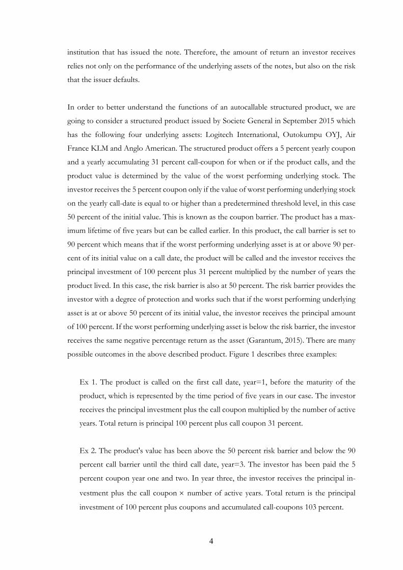
In order to better understand the functions of an autocallable structured product, we are

going to consider a structured product issued by Societe General in September 2015 which

has the following four underlying assets: Logitech International, Outokumpu OYJ, Air

France KLM and Anglo American. The structured product offers a 5 percent yearly coupon

and a yearly accumulating 31 percent call-coupon for when or if the product calls, and the

product value is determined by the value of the worst performing underlying stock. The

investor receives the 5 percent coupon only if the value of worst performing underlying stock

on the yearly call-date is equal to or higher than a predetermined threshold level, in this case

50 percent of the initial value. This is known as the coupon barrier. The product has a max-

imum lifetime of five years but can be called earlier. In this product, the call barrier is set to

90 percent which means that if the worst performing underlying asset is at or above 90 per-

cent of its initial value on a call date, the product will be called and the investor receives the

principal investment of 100 percent plus 31 percent multiplied by the number of years the

product lived. In this case, the risk barrier is also at 50 percent. The risk barrier provides the

investor with a degree of protection and works such that if the worst performing underlying

asset is at or above 50 percent of its initial value, the investor receives the principal amount

of 100 percent. If the worst performing underlying asset is below the risk barrier, the investor

receives the same negative percentage return as the asset (Garantum, 2015). There are many

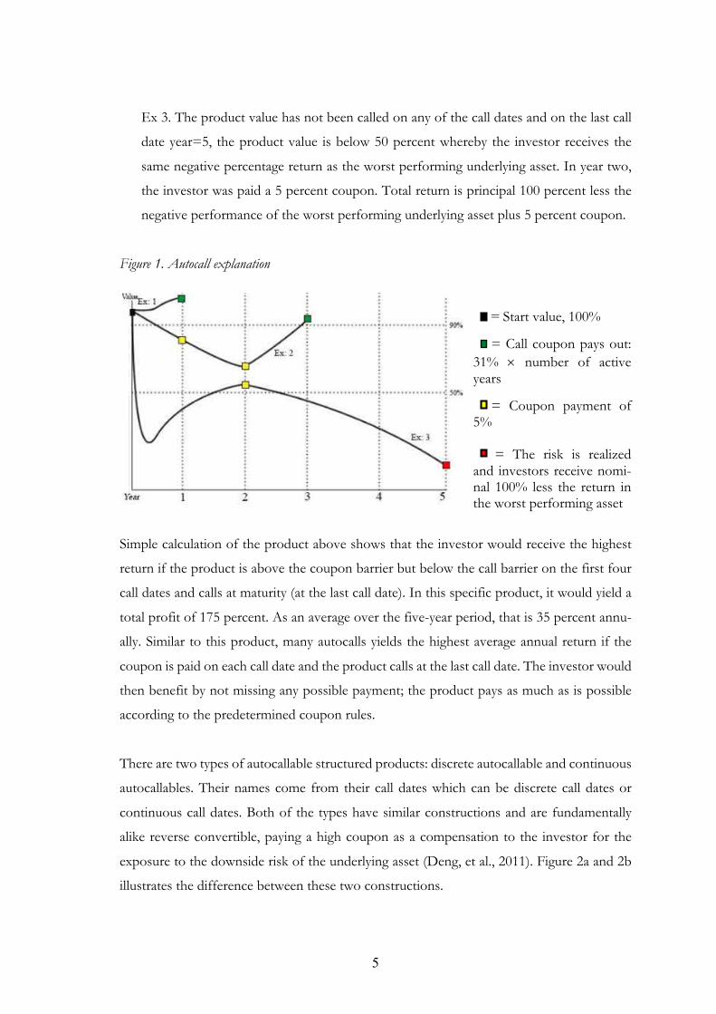
possible outcomes in the above described product. Figure 1 describes three examples:

Ex 1. The product is called on the first call date, year=1, before the maturity of the

product, which is represented by the time period of five years in our case. The investor

receives the principal investment plus the call coupon multiplied by the number of active

years. Total return is principal 100 percent plus call coupon 31 percent.

Ex 2. The product's value has been above the 50 percent risk barrier and below the 90

percent call barrier until the third call date, year=3. The investor has been paid the 5

percent coupon year one and two. In year three, the investor receives the principal in-

vestment plus the call coupon ´ number of active years. Total return is the principal

investment of 100 percent plus coupons and accumulated call-coupons 103 percent.

5

Ex 3. The product value has not been called on any of the call dates and on the last call

date year=5, the product value is below 50 percent whereby the investor receives the

same negative percentage return as the worst performing underlying asset. In year two,

the investor was paid a 5 percent coupon. Total return is principal 100 percent less the

negative performance of the worst performing underlying asset plus 5 percent coupon.

Figure 1. Autocall explanation

= Start value, 100% = Call coupon pays out: 31% ´ number of active years

= Coupon payment of 5% = The risk is realized and investors receive nomi-nal 100% less the return in the worst performing asset

Simple calculation of the product above shows that the investor would receive the highest

return if the product is above the coupon barrier but below the call barrier on the first four

call dates and calls at maturity (at the last call date). In this specific product, it would yield a

total profit of 175 percent. As an average over the five-year period, that is 35 percent annu-

ally. Similar to this product, many autocalls yields the highest average annual return if the

coupon is paid on each call date and the product calls at the last call date. The investor would

then benefit by not missing any possible payment; the product pays as much as is possible

according to the predetermined coupon rules.

There are two types of autocallable structured products: discrete autocallable and continuous

autocallables. Their names come from their call dates which can be discrete call dates or

continuous call dates. Both of the types have similar constructions and are fundamentally

alike reverse convertible, paying a high coupon as a compensation to the investor for the

exposure to the downside risk of the underlying asset (Deng, et al., 2011). Figure 2a and 2b

illustrates the difference between these two constructions.

6

Figure 2a and 2b: Discrete and continuous

Source: Deng, Mallett, McCann, 2011

In both figures we are analysing the same product. As illustrated, a discrete autocall can

only be called on predetermined dates, while a continuous autocall calls as soon as it

reaches the call barrier. In this study, we focus solely on discrete autocalls.

2.2 Creation Process of Structured Products

In order to create a structured product, there are a few key elements to take into considera-

tion. Pruchnicka-Grabias (2011) highlights three key elements: market situation, market fac-

tors and investors goal, which is shown in figure 3. There can be three different market

situations: bull, bear or a horizontal trend. Market factors to consider, amongst other, are

underlying assets volatility, interest rates and its volatility. An investors goal could be portfo-

lio diversification, capital protection or other. All of these elements must be considered to

balance risk and return.

As figure 3 shows, the general structured product has two components that generate the

return/profit of the product. The profit of a product is a combination of the return of the

fixed income instrument, and possible profits in the derivative due to volatility in the under-

lying assets (Braddock, 1997).

7

Figure 3: The process of the structured product creation

Source: Pruchnicka-Grabias (2011)

In selecting the underlying assets, there seems to be some common factors that are consid-

ered. Firstly, the underlying tends to be a well-known security, commonly a stock of a large

corporation. This is partly to increase the marketability of the product but also because stocks

and the options of large corporations tend to be more liquid which makes hedging less costly.

Furthermore, it is common to choose a stock with high dividend yield and to time the ma-

turity date of the product to shortly after a dividend payment. Since most types of structured

product do not take dividend payments in regard when valuing the product, the timing leads

to a price fall in the underlying asset shortly before the maturity date (Hernandez, 2007). This

lowers the products value and decrease the likelihood of the product calling in the call-date.

Recent research shows that at the time of issuance, a majority of the underlying assets have

a higher volatility than historically, adjusted for changes in the market volatility. This implies

that a majority of the underlying assets prices, at the point of issuance, tend to fluctuate more

than historically and it is not solely due to an increase in market volatility. Onwards, the

underwriter tends issue to products where the underlying, at the point of issuance, is close

to its 52-week high (Albuquerque et al. 2015). This is supported by Henderson and Pearson

(2011), who also emphasize that the derivatives value is an increasing function of the under-

lying assets volatility.

Furthermore, a key factor in the creation of structured products is represented by the credit

profile of the issuer. Generally, structured notes have been issued by investment and com-

mercial banks with high credit ratings. High-rated issuers are essential in order to isolate the

risk exposure desired by investors: investors in retail structured notes are generally searching

Market situation

Market factors

Investor´s goal

Creation of structured product

Fixed income instrument

Derivative

8

for an exposure to the underlying asset rather than the issuer’s credit risk. If the issuer be-

comes insolvent, the entire investment may be lost (Bergstresser, 2008).

2.3 Valuation Process of Autocallable Structured Products

How the structured product is constructed influences which method to use for valuation.

Pruchnicka-Grabias (2011) introduce a valuation method for a relatively simple construction:

a zero-coupon bond and an option. By separating the components of the product, it is pos-

sible to calculate a value of each, separately. Whereas the value of a zero-coupon can be

calculated with relative ease, it is more difficult to estimate the true value of the derivative.

The value of the bond can be calculated by the formula below, where 𝑃 represents the Price,

𝑌𝑇𝑀 represents the Yield to Maturity, 𝑡 represents the number of years to maturity and 𝐹𝑉

represents the Face Value.

𝑃 = !"($%&'(!)!

(1)

In order to calculate the value of an option, Pruchnicka-Grabias (2011) divides our option

in two elements: intrinsic value and time value. The intrinsic value is generally a measure of

what an asset is worth. However, here it represents the amount that the seller of the option

will have to pay if the option is exercised. The intrinsic value is affected by the option strike

price and the price of the underlying asset. For a call option, the intrinsic value is the under-

lying stock’s current price (USC) less the call strike price (CS). Reversibly, for a put option,

the intrinsic value is put option is the put strike prices (PS) minus USC. The time value

represents the amount of time left until maturity. A longer period of time until maturity will

result in a higher time value because there is a greater probability that the underlying assets

value changes thus increasing the intrinsic value. The time value is also influenced by the

volatility of the underlying assets price and interest rates, amongst other factors.

𝑂𝑝𝑡𝑖𝑜𝑛𝑣𝑎𝑙𝑢𝑒 = 𝐼𝑛𝑡𝑟𝑖𝑛𝑠𝑖𝑐𝑣𝑎𝑙𝑢𝑒 + 𝑇𝑖𝑚𝑒𝑣𝑎𝑙𝑢𝑒 (2)

Pruchnicka-Grabias (2011) further highlight that it is most common to use stock options,

index options and interest rate options to get exposure to the underlying asset. This is logical

considering that the majority of the underlying assets are equity and rates.

9

Amongst other valuation methods offered by academic literature are the simulation ap-

proach, the numerical integration approach, the decomposition approach and partial differ-

ential equations approach. Not all of the methods are effective in valuing all types of products

and some methods are hard to implement. Though, all four valuation methods take in con-

sideration and tries to price the risk of the underwriter defaulting, which may lead to the

investor losing the entire investment (Deng, et al. 2014).

2.4 Risks in an Autocall

Investing in autocalls presents the investor with a variety of risks. In order to properly un-

derstand the investment, the investor should consider all the risks, which include, but are not

limited to:

- Credit risks

- Construction risks

- Exposure risks

- Liquidity risks

- Market breakdown risks

The credit risk is the risk of the issuer goes insolvent. If the issuer is unable to honour its

obligation, that is to pay the investor the agreed return, the investor risks losing large parts

or all of the invested capital. This implies that the investor is not only exposed to the under-

lying asset that the product targets, but also to the default risk of the issuer. If the credit risk

is not appreciated, the expected value of the note will be overestimated (Henderson and

Pearson, 2011). If the credit rating of the issuing institution falls, the notes value on a sec-

ondary market may fall, as buyers in the secondary market may demand a higher risk pre-

mium due to increased risk of default.

Construction risk refers to the risk of missing out on return due to the construction of the

product. The product has a limited upside potential, the coupons, no matter how much the

underlying asset increase. In a strong bull market, therefore, the investor risks underperform

in relation to the market, due to the capped upside potential. Meanwhile, if the worst per-

forming underlying asset is below the risk barrier at maturity, the investor will be solely ex-

posed to the negative return of that asset and thereby has unlimited downside (Garantum,

2015)

10

The exposure risk is the exposure to the underlying asset(s). Since the development of the

underlying asset is determining the outcome of the product, it is important to understand

what influences the underlying assets value. The value is influenced by a variety of factors,

such as interest rates risks, stock price risks and political risks. An investment in the product

can yield a completely different return than an investment in the underlying asset(s). Partly

due to the construction risk, but also because any dividend paid by the underlying asset is

not accounted for in the return of the product (Garantum, 2015).

Selling the product before maturity may be difficult. It should, under normal market circum-

stances, not be a problem and as stated before, many issuer acts as market makers for their

products. The prices on the secondary market may be below the initial price and below the

products true value, depending on factors such as remaining time of the product, current

interest rates, credit ratings, market volatility. Under unnormal circumstances, it may be hard

or even impossible to sell the product (Garantum, 2015).

If the market “breaks down”, the characteristics of the product may change dramatically. It

could be because the trade in the underlying asset stops, the underlying asset no longer is

listed in a market or other reasons. In such situations, the issuer may change the terms as

they see fit due to the situation. It could be to replace the old underlying asset with a new or

change the way the return should be calculated which in turn changes the fundamentals of

the product (Garantum, 2015).

2.5 Valuation of Stocks

In our study, the entire sample consists of autocalls with equity as the underlying asset. Since

the stocks or index price determine the value of the product, it is important to know how

the return from stocks can be calculated.

When attempting to find the true value of a stock, one must consider a vast number of

different factors that may affect the price. The value of the stock is influenced by all factors

that affect the expectations of the future performance. These include factors that may be

unique to the specific firm but also factors that affect the entire industry or the entire econ-

omy (Reilly, 1973).

11

One academically acknowledged model for estimating the returns of a stock is the Capital

Asset Pricing Model (CAPM) in Equation 3. CAPM is an extension of Markowitz model of

portfolio choice (1959). Markowitz model suggests that the investor should chose a portfolio

of asset that will maximize expected return, given a level a variance or minimize the level of

variance, given a level of expected return. Sharpe (1964) and Lintner (1965) revised it and

added two key assumptions to the model. Firstly, an investor can borrow any amount of

money at a risk-free rate regardless on the amount already borrowed. Secondly, investors

have homogenous expectations on the probability of future returns. The formula is outlined

below, where 𝐸(𝑅!) represents the expected return of security 𝑖, 𝑅" represents the risk-free

rate, 𝛽! represents the Beta of security 𝑖 and 𝐸(𝑅#)represents the expected market return.

𝐸(𝑅!) = 𝑅" +𝛽!(𝐸(𝑅#) −𝑅") (3)

Where 𝛽! is a measure of the sensitivity in security 𝑖’s return to variation in market return. If

𝛽! =1, the security and the market are perfectly correlated (Elbannan, 2015). Despite the

model’s popularity and wide usage, empirical records indicate that the model is not perfect,

which is likely because of the many simplifying assumptions (Fama and French, 2004).

Another method to estimate the return of a security is through fundamental analysis.

Eiamkanitchat et al. (2017) describe the fundamental analysis approach as a three-layer top

down approach. Fundamental analysis firstly investigates the economy both globally and na-

tionally, by analysing financial data such as gross domestic product, interest rates and em-

ployment rates, to get an indication of whether the market is attractive or not. Secondly,

national industry data is analysed, using information such as price levels and different busi-

ness areas revenues, to find the most attractive sector. Once the most promising sector in

the most promising region has been identified, the analysis uses information such as profit

margins, earnings and return on equity, to find the most attractive stock. This approach has

several times been praised and the ratios that it uses are popular for attempting to predict the

future value of stocks. Basu (1983) finds that earnings-to-price (E/P) is positively related to

stock prices. Furthermore, Fama and French (1992) shows that stock prices are positively

related to book-to-market-price (B/P), i.e. the firm's own capital divided by the market value

of the firm. Stattman (1980) found that B/P is not only positively related to returns but also

12

to risk-adjusted returns and concludes that the B/P-ratio is an important ratio in predicting

a stock’s future price.

2.6 Hypothesis

Our hypothesis is that an increase in the return of the underlying assets will result in less than

equal increase in the returns of the autocall. We expect that one additional unit of return in

the variable 𝑠𝑡𝑜𝑐𝑘 will give less than one unit of increase in 𝐴𝐶: 𝛽$ < 1.

13

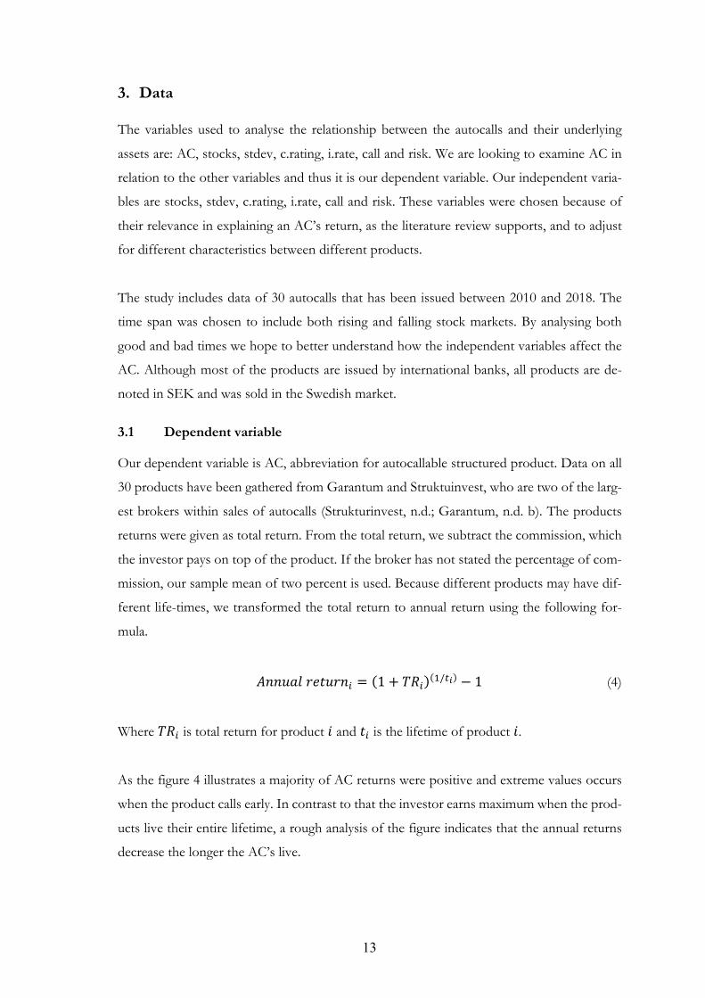
3. Data

The variables used to analyse the relationship between the autocalls and their underlying

assets are: AC, stocks, stdev, c.rating, i.rate, call and risk. We are looking to examine AC in

relation to the other variables and thus it is our dependent variable. Our independent varia-

bles are stocks, stdev, c.rating, i.rate, call and risk. These variables were chosen because of

their relevance in explaining an AC’s return, as the literature review supports, and to adjust

for different characteristics between different products.

The study includes data of 30 autocalls that has been issued between 2010 and 2018. The

time span was chosen to include both rising and falling stock markets. By analysing both

good and bad times we hope to better understand how the independent variables affect the

AC. Although most of the products are issued by international banks, all products are de-

noted in SEK and was sold in the Swedish market.

3.1 Dependent variable

Our dependent variable is AC, abbreviation for autocallable structured product. Data on all

30 products have been gathered from Garantum and Struktuinvest, who are two of the larg-

est brokers within sales of autocalls (Strukturinvest, n.d.; Garantum, n.d. b). The products

returns were given as total return. From the total return, we subtract the commission, which

the investor pays on top of the product. If the broker has not stated the percentage of com-

mission, our sample mean of two percent is used. Because different products may have dif-

ferent life-times, we transformed the total return to annual return using the following for-

mula.

𝐴𝑛𝑛𝑢𝑎𝑙𝑟𝑒𝑡𝑢𝑟𝑛! = (1 + 𝑇𝑅!)($/'!) − 1 (4)

Where 𝑇𝑅! is total return for product 𝑖 and 𝑡! is the lifetime of product 𝑖.

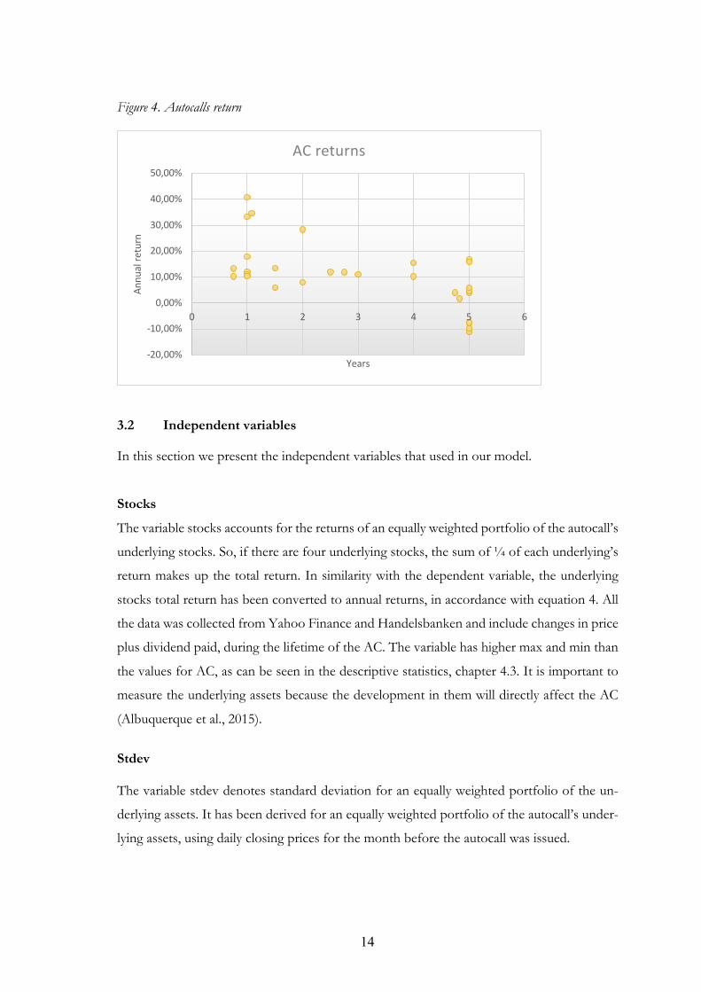
As the figure 4 illustrates a majority of AC returns were positive and extreme values occurs

when the product calls early. In contrast to that the investor earns maximum when the prod-

ucts live their entire lifetime, a rough analysis of the figure indicates that the annual returns

decrease the longer the AC’s live.

14

Figure 4. Autocalls return

3.2 Independent variables

In this section we present the independent variables that used in our model.

Stocks

The variable stocks accounts for the returns of an equally weighted portfolio of the autocall’s

underlying stocks. So, if there are four underlying stocks, the sum of ¼ of each underlying’s

return makes up the total return. In similarity with the dependent variable, the underlying

stocks total return has been converted to annual returns, in accordance with equation 4. All

the data was collected from Yahoo Finance and Handelsbanken and include changes in price

plus dividend paid, during the lifetime of the AC. The variable has higher max and min than

the values for AC, as can be seen in the descriptive statistics, chapter 4.3. It is important to

measure the underlying assets because the development in them will directly affect the AC

(Albuquerque et al., 2015).

Stdev The variable stdev denotes standard deviation for an equally weighted portfolio of the un-

derlying assets. It has been derived for an equally weighted portfolio of the autocall’s under-

lying assets, using daily closing prices for the month before the autocall was issued.

-20,00%

-10,00%

0,00%

10,00%

20,00%

30,00%

40,00%

50,00%

0 1 2 3 4 5 6

Annu

al re

turn

Years

AC returns

15

Portfolio theory suggests that the investor is not compensated for taking diversifiable or

unsystematic risk, such as firm-specific risks (Sharpe, 2000; Roy and Ghosh, 2012). However,

due to the creation of an autocall, the return of an investment in the product is dependent

on the volatility of the underlying assets. As Albuquerque et al (2015) found, a majority of

the underlying assets have higher volatility than historically, at the time of issuance of the

product. As described in the literature review, an investor may suffer a loss from investing

in the product, whilst earning a profit if that same investment would have been in the under-

lying assets.

Credit Rating The credit rating is the issuing institutions credit rating at the time of issuance. It has been

collected from the credit rating agency Moody´s. All products issuers have had a rating of

A1 or A2. Therefore, the variable c.rating is a dummy variable that takes on 0 if the issuer

has the higher grade of A1 and 1 if the issuer has the lower grade of A2.

As Bergstresser (2008) highlights, if the issuing institution goes insolvent, the investor may

lose the entire investment, regardless of the performance of the underlying assets. Therefore,

the credit rating becomes an important piece of information for the potential investor. If it

is not appreciated, the product will be overvalued (Henderson and Pearson, 2011).

Interest rate Data on the interest rate Statslåneräntan has been gathered from the Swedish National Debt

Office (Riksgälden, 2020). We have used the last published interest rate for the month of

issuance for the respective product. During a majority of the examination period, the national

interest rate has been in a falling trend until around 2015, where it starts moving sideways at

around 0 – 0.5 percent.

In the construction of an autocall, the issuer uses bonds, as described in the literature review.

When interest rates fall, the bonds value generally increase (SEC, n.d.). Deng et al (2014)

shows that if the bonds value increase, so does the face value of the product. Further, with

falling interest rates, investors seek returns in riskier assets such as stocks. The inflow of

capital to the stock market can be a contributing factor to rising stock prices (Stoica et al.

16

2014). Since both bonds and derivatives of stocks are in the construction of a structured

products, we have included it to find out how it is related to our sample.

Call barrier and Risk barrier To compensate for differences in the characteristics of different autocalls, we have included

the call and risk barrier for each product. From our sample, both variables only take on two

values and are therefore constructed as dummy variables.

The call barrier is either 90 percent or 100 percent of the start value. If the call barrier is 90

percent, the dummy variable is 1 and if the barrier is 100 percent, the variable is 0. Similarly,

for the risk barrier, it only takes two values. The variable takes on the value 1 if the risk

barrier is 50 percent and 0 if the risk barrier is 60 percent.

Although no identified study has examined how much the difference in call and risk barriers

affect the return of the autocall, several studies highlight the barriers importance in deciding

the return to be paid to the investor (Hansson, 2012; Hunt, 2015; Albuquerque et al., 2015).

17

4. Method

To analyse the relationship between the returns of an AC and its underlying asset and test

the hypothesis, several methods complementing each other was used. Our hypothesis is con-

firmed if the variable 𝛽$ < 1. That is, if stock increase by one unit, AC increases less than

one unit, keeping the other variables fixed. If 𝛽$ < 1 with a p-value below 0.05, we accept

our hypothesis and conclude that an increase in the underlying assets results in a less than

equal increase in the autocall’s returns.

4.1 Quantitative research

The quantitative research was formed to analyse the data of the variables using several econ-

ometrics approaches. Data was collected from two brokers of autocalls, Yahoo Finance and

Handelsbanken, the credit rating agency Moody´s, and the Swedish National Debt Office.

The data is analysed through a cross-section regression analysis. We have chosen Ordinary

Least Squares (OLS) regression to make the analysis. Following the regression, a number of

tests were performed to identify any unwanted symptoms in the data set. This is further

discussed under Methodology 4.2.

The model we have chosen to analyse the issue is the following:

𝐴𝐶! = 𝛼 + 𝛽$𝑠𝑡𝑜𝑐𝑘𝑠! + 𝛽)𝑠𝑡𝑑𝑒𝑣! + 𝐷$𝑐. 𝑟𝑎𝑡𝑖𝑛𝑔! + 𝛽*𝑖. 𝑟𝑎𝑡𝑒! + 𝐷)𝑐𝑎𝑙𝑙! + 𝐷*𝑟𝑖𝑠𝑘! +𝑢! (5)

𝛼 =intercept

𝑢! = error term

𝑖 = cross sectional identifier (AC 1, 2, ..., 30)

The variable 𝐴𝐶! is our dependent variable and variables 𝑠𝑡𝑜𝑐𝑘𝑠! , 𝑠𝑡𝑑𝑒𝑣! , 𝑐. 𝑟𝑎𝑡𝑖𝑛𝑔! ,

𝑖. 𝑟𝑎𝑡𝑒! , 𝑐𝑎𝑙𝑙! and 𝑟𝑖𝑠𝑘! are our explanatory variables. The variables are discussed in Data

3.2.

4.2 Methodology

To ensure that the none of the classical OLS assumptions were violated, a series of diagnos-

tics tests were run.

18

Having run our main OLS regression, we tested it for heteroscedasticity. This was done using

the Breusch-Pagan-Godfrey test. The presence of heteroscedasticity causes a problem be-

cause OLS regression assumes that the residuals comes from a population with constant

variance (homoscedasticity). With heteroscedasticity present, the OLS estimators would be

inefficient but not biased (Gujarati and Porter, 2009). The results are presented in Appendix

A and show that the residuals are homoscedastic and thus there is no presence of heterosce-

dasticity.

Furthermore, the regression was investigated for autocorrelation. Autocorrelation or serial

correlation refers to correlated error terms and if caused by e.g. an omitted variable or model

misspecification, it leads to biased estimators (Gujarati and Porter, 2009). In our case, the

Durbin-Watson d-test would not be accurate in determining if there is a problem of auto-

correlation or not. This is because our d-statistics fall in the “zone of indecision”. Instead,

this was done using the Breusch-Godfrey LM test with the lag-length that minimize Akaike

Info Criterion (AIC), in this case one lag. The results are presented in Appendix B and show

that there is no serial correlation.

Onwards, the data set is examined for high levels of correlation using a correlation matrix.

Considering that the model contains a number of variables, multicollinearity could be a prob-

lem. To avoid multicollinearity, we used the Variance Inflating Factor (VIF) method, further

explained in chapter 4.5.

4.3 Descriptive statistics

Table 1. Descriptive statistics AC % Stocks % Stdev % C.rating I.rate% Risk Call Mean 10.27 16.93 29.40 0.80 1.36 0.70 0.40 Median 10.73 11.63 23.00 1.00 1.51 1.00 0.00 Max 41.00 58.37 60.10 1.00 2.87 1.00 1.00 Min -10.93 -7.17 9.70 0.00 0.00 0.00 0.00 Std.dev. 12.80 18.00 15.20 40.69 0.78 46.61 49.83 Number of ob-servations 30 30 30 30 30 30 30

Table 2 shows the descriptive statistics for all the variables. All variables have the same num-

ber of observations, 30, and thereby the data set is complete. As previously mentioned, the

19

stocks return have a higher max and a higher min than the autocalls. The stocks return also

have notable higher standard deviation than the autocall’s return.

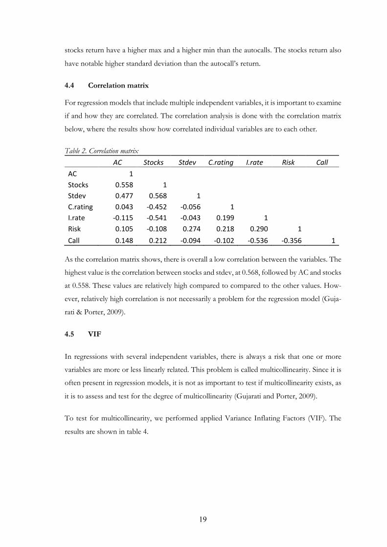
4.4 Correlation matrix

For regression models that include multiple independent variables, it is important to examine

if and how they are correlated. The correlation analysis is done with the correlation matrix

below, where the results show how correlated individual variables are to each other.

Table 2. Correlation matrix

AC Stocks Stdev C.rating I.rate Risk Call AC 1 Stocks 0.558 1 Stdev 0.477 0.568 1 C.rating 0.043 -0.452 -0.056 1 I.rate -0.115 -0.541 -0.043 0.199 1 Risk 0.105 -0.108 0.274 0.218 0.290 1 Call 0.148 0.212 -0.094 -0.102 -0.536 -0.356 1

As the correlation matrix shows, there is overall a low correlation between the variables. The

highest value is the correlation between stocks and stdev, at 0.568, followed by AC and stocks

at 0.558. These values are relatively high compared to compared to the other values. How-

ever, relatively high correlation is not necessarily a problem for the regression model (Guja-

rati & Porter, 2009).

4.5 VIF

In regressions with several independent variables, there is always a risk that one or more

variables are more or less linearly related. This problem is called multicollinearity. Since it is

often present in regression models, it is not as important to test if multicollinearity exists, as

it is to assess and test for the degree of multicollinearity (Gujarati and Porter, 2009).

To test for multicollinearity, we performed applied Variance Inflating Factors (VIF). The

results are shown in table 4.

20

Table 3. Variance Inflating Factors

Variables Coefficients Variance Uncentered VIF Centered VIF

Intercept 0.0082 24.8981 NA STOCKS 0.0352 6.3962 3.3374 STDEV 0.0314 10.3432 2.1178 CRATING 0.0029 7.1281 1.4256 IRATE 12.2662 9.0495 2.1725 CALL 0.0021 2.5181 1.5108 RISK 0.0021 4.4297 1.3289

Interpreting the table above, the centered VIF should be close to 0 for very low multicollin-

earity. To ensure no multicollinearity, the centered VIF should be below 10 (Lin, 2008). As

the table shows, all variables are below 10 and we therefore conclude that there is no multi-

collinearity present.

21

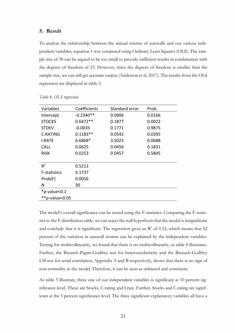
5. Result

To analyse the relationship between the annual returns of autocalls and our various inde-

pendent variables, equation 1 was computed using Ordinary Least Squares (OLS). The sam-

ple size of 30 can be argued to be too small to provide sufficient results in combination with

the degrees of freedom of 23. However, since the degrees of freedom is smaller than the

sample size, we can still get accurate output (Anderson et al, 2017). The results from the OLS

regression are displayed in table 5.

Table 4. OLS regression

Variables Coefficients Standard error Prob. Intercept -0.2340** 0.0906 0.0166 STOCKS 0.6472** 0.1877 0.0022 STDEV -0.0035 0.1771 0.9875 C.RATING 0.1183** 0.0542 0.0395 I.RATE 6.6868* 3.5023 0.0688 CALL 0.0625 0.0456 0.1831 RISK 0.0253 0.0457 0.5845

R2 0.5213 F-statistics 4.1737 Prob(F) 0.0056 N 30 *p-value<0.1 **p-value<0.05

The model’s overall significance can be tested using the F-statistics. Comparing the F-statis-

tics to the F-distribution table, we can reject the null hypothesis that the model is insignificant

and conclude that it is significant. The regression gives an R2 of 0.52, which means that 52

percent of the variation in autocall returns can be explained by the independent variables.

Testing for multicollinearity, we found that there is no multicollinearity, as table 4 illustrates.

Further, the Breusch-Pagan-Godfrey test for heteroscedasticity and the Bresuch-Godfrey

LM test for serial correlation, Appendix A and B respectively, shows that there is no sign of

non-normality in the model. Therefore, it can be seen as unbiased and consistent.

As table 5 illustrate, three one of our independent variables is significant at 10 percent sig-

nificance level. These are Stocks, C.rating and I.rate. Further, Stocks and C.rating are signif-

icant at the 5 percent significance level. The three significant explanatory variables all have a

22

positive coefficient sign, meaning that an increase in any of the variables, holding all the other

explanatory variables constant, would increase the dependent variable. A one unit increase

in the variable Stocks, holding the others constant, would increase autocalls by 0.647 units.

If the dummy variable C.rating is one, that is if the issuer has the lower credit rating of A2,

the dependent variable is positively affected by 0.118 units. A one unit increase in I.rate

would cause an increase in the dependent variable by 6.687 units.

According to the regression output, the variables standard deviation and the dummy varia-

bles call -and risk barrier are insignificant. This means that we cannot conclude that these

three variables have a sustainable effect on the dependent variable.

23

6. Analysis

The results in table 5 show that stocks positively affect the autocall’s return. According to

the model, a one unit increase in the stocks return increases autocall’s return by 0.6472 units

keeping the other variables constant. This confirms our hypothesis that 𝛽$ < 1. The positive

relation between the variables is in line with the products construction and previous research

(Garantum 2015; Albuquerque et al., 2015). An increase in the underlying stocks should lead

to an increase in the autocall’s returns since the value of the underlying stocks are the primary

determinants for the autocall’s value. Therefore, if the value of the underlying stocks rises,

the return of the autocall rise as it is a higher chance that the product is in any payoff zone,

to pay either the regular coupon or the call-coupon. However, our results show that this is

true also in reverse. If the return of the underlying falls by one unit, the return of the autocall

falls with less than one unit, which is likely due to the risk-barrier offering a degree of pro-

tection.

As Pruchnicka-Grabias (2011) describes, most structured products are constructed using a

fixed income instrument, as a bond, and a derivative instrument, such as options. Further,

Hernandez (2007) found that most structured products are constructed so that the call date

is shortly after the dividend payout and Albuquerque et al. (2015) shows that the underlying

assets volatility versus historical volatility is higher at the time of issuance, adjusted for in-

creases in market volatility. Since the autocall does not account for dividend in the underlying

assets, the autocall’s value will fall when the underlying assets pay dividend. This in turn,

when timed so that the call-date is shortly after the dividend payout, decreases the chance of

the product giving a coupon payment since the value of the product drops shortly before the

call date.

With higher volatility, the risk of the AC being under the coupon barrier or over the call

barrier on any of the call dates would be higher than if the underlying asset was less volatile.

Likewise, the risk of the underlying asset being below the risk barrier at maturity, potentially

resulting in a loss for the investor, is higher if the underlying assets have high volatility com-

pared to assets with low volatility. Therefore, higher volatility in the underlying assets can be

harmful for the autocall’s return. Whilst the product may suffer from increased volatility, the

derivative, normally options, used to construct the product tend to increase in price as vola-

tility rises (Braddock, 1997; Henderson and Pearson 2011). The volatility can thereby be an

influencing factor on the issuers profit, which could be why most products underlying have

24

higher volatility at issuance compared to historically and adjusted for changes in market vol-

atility (Albuquerque et al., 2015). Recalling that it is only the worst performing asset that

determines the products value, it does not matter if three of the four underlying assets double

in value, if the fourth asset has lost half of its value. The output in table 5 for the variable

Stdev shows that there is a negative relation between it and the dependent variable. However,

the variable is highly insignificant which is why we cannot draw any conclusions from it.

The results from the regression model shows that credit rating has a significant effect on the

dependent variable. If the credit rating is the lower rating of A2, the return in the autocall

increases. Henderson and Pearson (2011) found that if the credit risk is not appreciated

properly, the value of the product will be overestimated. With an overestimated value, the

return should be lower than with a fairly valued product. Investors in retail structured notes

are generally searching for an exposure to the underlying asset rather than the issuer’s credit

risk. If the issuer defaults, the entire investment may be lost, regardless of the performance

in the underlying assets (Bergstresser, 2008). Therefore, if the issuer has a lower credit rating,

investors may demand an extra compensation for the extra credit risk they take on by invest-

ing in the product. Due to that our data does not cover any major financial crises, the risk of

the issuer going default may not have been realized. Thus, investors investing in products

issued by a lower rated institution may have enjoyed the higher return without experiencing

the risk of default realized. Expanding the data to cover the financial crises of 2008 may give

a different result since it can be harder for lower rated institutions to, in such circumstances,

meet their obligations, compared to higher rated institutions.

From the output in table 5, interest rate is shown to have a strong positive effect of the

autocall’s returns. A one-unit increase would increase the dependent variable by 6.69 units.

With bonds normally representing the fixed income instrument in the product (Pruchnicka-

Grabias, 2011), interest rate ought to affect the products value. With falling interest rates, the

bonds value generally increases (SEC, n.d.). Deng et al (2014) shows that the face value of

the product increase if the bonds value increase. Further, another consequence of falling

interest rate is that the return from investing in safe assets, such as savings accounts or high

rated bonds, falls. In search of returns, investors are forced to find alternative assets, such as

stocks, to invest in. Therefore, with falling interest rates, previous studies have found a large

capital inflow to the stock market which in turn increases stock prices (Stoica et al. 2014).

Our results, that if interest rate rise – so does the return in the autocall, are in contradiction

25

with this. This is likely due to that in the data, the interest rate is observed only at the issuance

of the product. Therefore, our model cannot explain how a specific product’s value change

due to changes in interest rate. Rather it describes the change of the returns between different

products, given the interest rate at issuance.

Analysing the dummy variable call, we find that if the call-barrier is 90 percent, the dependent

variable increases by 0.0625 with all other variable's constant. This follows the rationale that

with a lower call barrier, there is a higher probability of the product calling (Deng et al., 2011).

With a higher probability of calling, the investor may expect a higher payoff. However, the

regression results show that the variable is insignificant and therefore we cannot draw a con-

clusion on how the variable effects the autocall’s return in this sample.

The risk barrier is in similarity with the call barrier a dummy variable, that equals 1 if the risk

barrier is 50 percent and 0 if it is 60 percent. From the table 5, we observe that if the risk

barrier is 50 percent, the dependent variable increases by 0.0253 units, keeping all other var-

iables constant. The risk barrier protects the investor in such way that if the worst performing

underlying asset is above it when the product reaches maturity, the investor is paid back his

principle investment. It therefore follows a similar rationale as described for the call-barrier,

that if the risk-barrier is 50 percent rather than 60 percent, the investor enjoys an extra pro-

tection-area of 10 percentage points. Hansson (2012) argues that there is a low probability

of ending up in the risk barrier zone and because the risk-variable, just as the call variable, is

insignificant, we cannot conclude that it has a positive effect on the dependent variable.

6.1 Limitations

This thesis has been an explorative study, as much of the previous research has not primarily

focused on how the underlying assets returns affect the autocall’s return, but rather different

autocall valuation methods. As with many research papers, there are limitations to the study

and its analysis. One of the limitations is the inaccessibility of data on regular closing prices

of the autocalls to calculate the volatility of its price. We believe that with access to such data,

a more thorough analysis can be made. Another limitation is the lack of data before 2010.

Investigating products issued between 2010 and 2018 does not allow us to draw any conclu-

sion of how a deep financial crisis would affect the variables in the model. Unfortunately,

these are both factors we have been unable to affect during the writing of this thesis. Despite

these limitations, we believe that the overall quality is adequate.

26

7. Conclusion

The purpose of this thesis was to investigate the relationship between an autocall and its

underlying assets. Specifically, we wanted to find if an increase in the return of the stocks

would result in a higher, same or lower return in the autocall. Our results allow us to confirm

our hypothesis: an increase in value the underlying assets is not followed by an equal increase

in the products value. Despite our findings, autocalls can be an interesting alternative invest-

ment that can provide the investor with a safety net as well as diversification.

When deciding whether to invest in an autocallable structured product, the investor must

consider several risks. Even if the returns in the products are ultimately governed by the

development of the underlying assets, the investor must consider other risks such as the

issuers credit status and liquidity risks. Based on the result in our quantitative analysis, we

can conclude that there is a significant link between the performance of an autocall and an

equally weighted portfolio of its underlying assets. An increase in the stocks return, holding

the other independent variables constant, does not result in an equally large increase in the

autocall.

With regards to the other variables in the model, apart from the underlying stocks, the credit

rating of the issuing institution and the interest rate at the time of issuance proved to have a

significant effect on the dependent variable. Whilst some of the variables relation to the

dependent variable follow previous research and theories, others had not been discussed in

the same extent.

For future research within the subject, it would be interesting to expand the timeframe so

that it includes a financial crises or recession, in order to better understand how the variables

relate to each other under extreme market situations. With access to data on the secondary

market-pricing of autocalls, future research could also examine how their prices change over

time to better understand the risk of the products. Examining price change, it would be

interesting to see how the return in the autocall is related to its standard deviation. Further,

it would be of interest to conduct a panel data analysis to examine differences in returns

between countries and across time, preferably including data on one or more crisis. This

would highlight differences within geographical markets as well as explain how the products

return develop throughout both good and bad times.

27

Reference list

Albuquerque, R., Gaspar, R.M. and Michel, A. CFA Institute. (2015). “Investment Analysis

of Autocallable Contingent Income Securities.” Financial Analysts Journal, 71(3), 61-83

Anderson, D., Freeman, J., Shoesmith, E., Sweeney, D. and Williams, T. (2017). Statistics for

business and economics (4th ed.). Boston, MA: South-Western Cengage learning.

Basu, S. (1983). The relationship between earnings' yield, market value and return for NYSE

common stocks: Further evidence. Journal of Financial Economics, 20(1), 129-156.

Braddock, J.C. (1997). Derivatives Demystified – Using Structured Financial Products, John

Wiley & Sons, Chichester

Das, S. (2000). Structured Products and Hybrid Securities, John Wiley & Sons, Singapur

Deng, G., Husson, T. and Mccann, C. (2014). Valuation of Structured Products. Journal of

Alternative Investments. 16.

Deng, G., Mccann, C. and Mallett, J. (2011). Modeling Autocallable Structured Products.

Journal of Derivatives & Hedge Funds. 17. 326-340.

Deutscher Derivate Verband. (2019). The German Derivatives Market, June 2019. Accessed

February 12, 2020, from: https://www.derivateverband.de/ENG/Statistics/MarketVolume

Eiamkanitchat, N., Moontuy, T. and Ramingwong, S. (2017). Fundamental analysis and tech-

nical analysis integrated system for stock filtration. Cluster Computing. 20(1), 883–894.

Elbannan, M. (2015). The Capital Asset Pricing Model: An Overview of the Theory. Interna-

tional Journal of Economics and Finance, 7(1), 216–228.

EUSIPA. (2019). Q2 2019 Market Report Update. Accessed February 12, 2020, from:

https://eusipa.org/eusipa-publishes-q2-2019-market-report-update/

Fama, E.F. and French, K.R. (2004). The Capital Asset Pricing Model: Theory and Evidence.

The Journal of Economic Perspectives, 18(3) 25–46.

28

Fama, E.F. and French, K.R. (1992), The Cross-Section of Expected Stock Returns. The

Journal of Finance, 47: 427-465.

Finansinspektionen. (2019). Accessed February 10, 2020, from

https://www.fi.se/contentassets/1b9c05e28c7b4f19b32b57b4f04b3fec/konsument-

skyddrapport-2019ny.pdf).

Finansinspektionen. (2014). Konsumentskyddsrapport 2019. Accessed February 13, 2020,

from https://www.fi.se/sv/publicerat/fi-forum/2014/strukturerade-produkter-och-kon-

sumentskydd/

Garantum. n.d. Accessed February 16, 2020, from https://www.garantum.se/Produktinfor-

mation/sa-fungerar-det/sa-fungerar-andrahands-brmarknaden/

Garantum. n.d. b. Accessed May 3, 2020, from https://www.garantum.se/Om-

Garantum/om-oss/kort-om-garantum/

Garantum. (2015). SG AC Europeiska bolag Combo 2373. Accessed February 18, 2020,

from https://www.garantum.se/Produktinformation/Aktuell-emission/Products/2015-

September/SG-AC-Europeiska-bolag-Combo-2373/#MarketValues

Gujarati, D. and Porter, C. (2009). Basic Econometrics (5th ed.). New York, NY: McGraw-

Hill Irwin.

Hansson, F. (2012). A pricing and performance study on auto-callable structured products.

KTH Royal Institute of Technology. Accessed March 14, 2020, from:

https://www.math.kth.se/matstat/seminarier/reports/M-exjobb12/120528.pdf

Henderson, B.J. and Pearson, N.D. (2011). “The Dark Side of Financial Innovation: A Case

Study of the Pricing of a Retail Financial Product.” Journal of Financial Economics, vol. 100, no.

2 (May): 227–247.

29

Hernandez, R.J. (2007). An economic analysis of structured products, University of Arkan-

sas. Accessed March 12, 2020, from: https://search-proquest-com.proxy.library.ju.se/cen-

tral/docview/304897561/79B9712B2BA44CE9PQ/1?accountid=11754

Hunt, S., Stewart, N. and Zaliauskas, R. (2015). Two plus two makes five? Survey evidence

that investors overvalue structured deposits. Financial Conduct Authority. Occasional Paper

No.9

Investing. (2020). Accessed February 18, 2020, from: https://se.investing.com/indices/us-

spx-500

Lin, F.J. (2008). Solving multicollinearity in the process of fitting regression model using the

nested estimate procedure. Quality and Quantity, 42(3), 417-426.

Lintner, J. (1965). The Valuation of risk assets and the selection of risky investments in stock

portfolios and capital budgets. The Review of Economics and Statistic, 47(1).

Markowitz, H. (1952). Portfolio selection. Journal of Finance, 7(1), 77–99.

Mellqvist, G. (2017). ‘Flera profiler varnar efter DI:s artiklar om Nordea’. Dagens Industri,

January 5, 2017. Accessed February 10, 2020, from

https://www.di.se/nyheter/flera-profiler-varnar-efter-dis-artiklar-om-nordea/

Pruchnicka-Grabias, I. (2011). Dilemmas of structured products valuation. Contemporary Legal

and Economic Issues, 3, 238–251.

Reilly, F.F. (1973). MISDIRECTED EMPHASIS IN STOCK VALUATION. Financial An-

alysts Journal, 29(1), 54.

Riksgälden. (2020). Accessed March 25, 2020, from https://www.riksgalden.se/sv/var-

verksamhet/statslanerantan/statslanerantan-per-vecka/

Roy, S. and Ghosh, S. K. (2012). Portfolio construction and the reduction of diversifiable

risk. International Journal of Financial Management, 2(4), 60-70.

30

SEC. n.d. Accessed May 1, 2020, from https://www.sec.gov/files/ib_interestraterisk.pdf

Sharpe W. F. (2000). Portfolio Theory and Capital Markets. McGraw-Hill, New York.

Sharpe, W. F. (1964). Capital asset prices: A theory of market equilibrium under conditions

of risk. Journal of Finance, 19(3), 425–442.

Stattman, D. (1980). Book values and stock returns. The Chicago MBA, 4, 25. Accessed April

12, 2020 from: http://proxy.library.ju.se/login?url=https://search-proquest-com.proxy.li-

brary.ju.se/docview/233201765?accountid=11754

Stoica, O., Nucu, A. and Diaconasu, D. (2014). Interest Rates and Stock Prices: Evidence

from Central and Eastern European Markets. Emerging Markets. Finance & Trade, 50.

Strukturinvest. n.d. Accessed May 3, 2020, from https://strukturinvest.se/om-strukturin-

vest/om-strukturinvest.aspx

Suneson. (2009). ‘Hur säkra är dina pengar?’, Svenska Dagbladet, April 14, 2009. Accessed

March 1, 2020, from https://www.svd.se/hur-sakra-ar-dina-penga

31

Appendix

Appendix A. BPG-test Table 5. BPG-test Breusch-Pagan-Godfrey test for heteroscedasticity F-statistic 0.625632 Prob. F(6,23) 0.7081 Obs*R-squared 4.209263 Prob. Chi-squared(6) 0.6484 Scaled explained SS 3.516412 Prob. Chi-squared(6) 0.7418

Appendix B. BG-test Table 6. BG-test Breusch-Godfrey LM test for serial correlation (up to 1 lag) F-statistic 1.869993 Prob. F(1,22) 0.1853 Obs*R-squared 2.350222 Prob. Chi-squared(1) 0.1253