Author's personal copy - ERNETrajibmaity/JH_Streamflow prediction...Author's personal copy Stream ow...

This article appeared in a journal published by Elsevier. The attachedcopy is furnished to the author for internal non-commercial researchand education use, including for instruction at the authors institution

and sharing with colleagues.

Other uses, including reproduction and distribution, or selling orlicensing copies, or posting to personal, institutional or third party

websites are prohibited.

In most cases authors are permitted to post their version of thearticle (e.g. in Word or Tex form) to their personal website orinstitutional repository. Authors requiring further information

regarding Elsevier’s archiving and manuscript policies areencouraged to visit:

http://www.elsevier.com/copyright

http://www.elsevier.com/copyright

Author's personal copy

Streamflow prediction using multi-site rainfall obtained from hydroclimaticteleconnection

S.S. Kashid a, Subimal Ghosh a,⇑, Rajib Maity b

a Department of Civil Engineering, Indian Institute of Technology Bombay, Powai, Mumbai 400 076, Indiab Department of Civil Engineering, Indian Institute of Technology Kharagpur, Kharagpur 721 302, West Bengal, India

a r t i c l e i n f o

Article history:Received 6 February 2010Received in revised form 21 September2010Accepted 4 October 2010

This manuscript was handled byK. Georgakakos, Editor-in-Chief, with theassistance of Ercan Kahya, Associate Editor

Keywords:El Niño Southern Oscillation (ENSO)Equatorial Indian Ocean Oscillation(EQUINOO)Outgoing Longwave Radiation (OLR)Mahanadi RiverGenetic ProgrammingHydroclimatic teleconnection

s u m m a r y

Simultaneous variations in weather and climate over widely separated regions are commonly known as‘‘hydroclimatic teleconnections’’. Rainfall and runoff patterns, over continents, are found to be signifi-cantly teleconnected, with large-scale circulation patterns, through such hydroclimatic teleconnections.Though such teleconnections exist in nature, it is very difficult to model them, due to their inherent com-plexity.

Statistical techniques and Artificial Intelligence (AI) tools gain popularity in modeling hydroclimaticteleconnection, based on their ability, in capturing the complicated relationship between the predictors(e.g. sea surface temperatures) and predictand (e.g., rainfall). Genetic Programming is such an AI tool,which is capable of capturing nonlinear relationship, between predictor and predictand, due to its flexiblefunctional structure. In the present study, gridded multi-site weekly rainfall is predicted from El NiñoSouthern Oscillation (ENSO) indices, Equatorial Indian Ocean Oscillation (EQUINOO) indices, OutgoingLongwave Radiation (OLR) and lag rainfall at grid points, over the catchment, using Genetic Programming.

The predicted rainfall is further used in a Genetic Programming model to predict streamflows. Themodel is applied for weekly forecasting of streamflow in Mahanadi River, India, and satisfactory perfor-mance is observed.

� 2010 Elsevier B.V. All rights reserved.

1. Introduction

Basin-scale streamflow prediction is an important step inwater resources management for sustainable development. Thevariation of basin-scale streamflow is influenced by rainfall depth,its distribution pattern, catchment characteristics and the groundwater contribution to the streamflow. The rainfall distribution,over the catchment, depends on local meteorology, large scaleatmospheric circulation patterns and the geography of the catch-ment. It may be difficult to predict weekly streamflow accurately,by just considering the rainfall of few previous weeks, because therainfall in current week also has substantial contribution tostreamflow. This is especially true for monsoon season, whenthe soil is saturated, leading to insignificant infiltration. In thepresent study, a two-step approach is proposed for weeklystreamflow prediction. In first step, current (weekly) multi-grid-ded rainfall is predicted with Genetic Programming (GP), basedon large scale atmospheric circulation patterns, OLR and lag rain-fall at grid points. Current step weekly streamflow is then pre-dicted, by using observed gridded rainfall, up to previous

weekly time step and GP predicted multi-gridded rainfall, at cur-rent weekly time step.

A single step model, for streamflow forecasting, is also devel-oped, by using same inputs and the results are compared withthe performance of two step model.

The objectives of this study are summarized as following:

(1) To develop GP-based models, for weekly multi-site(multi-gridded) rainfall prediction, based on large scaleatmospheric circulation patterns with hydroclimatic tele-connection, lag multi-gridded rainfall and OLR.

(2) To develop GP-based weekly basin-scale streamflow predic-tion model, based on observed gridded rainfall at few previ-ous weekly time steps, GP predicted gridded rainfall atcurrent time step and lagged streamflow at immediate pre-vious weekly time step.

(3) To assess the improvement in streamflow predictions due toinclusion of current step (week), GP predicted rainfall in theinput set, in addition to the observed gridded rainfall up tothe lag-1 weekly time step.

(4) To compare the results of the aforesaid two-step model witha single-step model, that uses lag streamflow, ENSO indices,EQUINOO indices, OLR anomaly, historical avg. rainfall andrainfall at the all grid points over last six weeks.

0022-1694/$ - see front matter � 2010 Elsevier B.V. All rights reserved.doi:10.1016/j.jhydrol.2010.10.004

⇑ Corresponding author. Tel.: +91 22 2576 7319 (Off.), +91 22 2576 8319 (Res.).E-mail addresses: [email protected], [email protected] (S. Ghosh).

Journal of Hydrology 395 (2010) 23–38

Contents lists available at ScienceDirect

Journal of Hydrology

journal homepage: www.elsevier .com/ locate / jhydrol


The methodology adopted for streamflow prediction in the two-step model can be visualized in flowchart (Fig. 1a). The first stepdeals with the multi-gridded rainfall prediction, and the secondstep deals with the basin-scale streamflow prediction.

Similarly the methodology of a single-step model can be seen inflowchart (Fig. 1b).

The rainfall as well as streamflow-prediction models are devel-oped by using Genetic Programming tool. The methodology is dif-ferent from the methodologies mentioned in the literature (Eltahir,1996; Piechota et al., 1997; Chiew et al., 1998; Chandimala andZubair, 2007).

The novelty of this method lies in the inclusion of predictedcurrent week rainfall in streamflow-prediction model thatcontributes to current-week streamflow, especially in monsoonseason.

2. Influence of large scale atmospheric circulation patterns overspatio-temporal rainfall distribution

Simultaneous variations in weather and climate over widelyseparated regions on earth have long been noted in the meteoro-logical literature. Such recurrent patterns are commonly referredas ‘‘teleconnections’’. Rainfall distribution patterns over the conti-nents are significantly linked with the atmospheric circulationthrough hydroclimatic teleconnection.

It is also established that the natural variation of rainfall islinked with these large scale atmospheric circulation patterns,through hydroclimatic teleconnection (Dracup and Kahya, 1994;Eltahir, 1996; Jain and Lall, 2001; Douglas et al., 2001; Ashoket al., 2004; Marcella and Eltahir, 2008; Maity and Nagesh Kumar,2006, 2008). Hydroclimatic teleconnection between Indian Sum-mer Monsoon Rainfall and large scale atmospheric circulation pat-terns over Pacific Ocean and Indian Ocean was established inliterature (Rasmusson and Carpenter, 1983; Parthasarathy et al.,1988; Krishna Kumar et al., 1999; Ashok et al., 2001; Li et al.,2001; Gadgil et al., 2003, 2004; Maity and Nagesh Kumar, 2006).

El Niño Southern Oscillation (ENSO) is the coupled ocean–atmo-sphere mode of variability in the tropical Pacific Ocean (Cane,1992), whereas Indian Ocean Dipole (IOD) mode is the same overtropical Indian Ocean (Saji et al., 1999). El Niño Southern Oscilla-tion (ENSO) is related to ocean–atmosphere interaction in theequatorial Pacific Ocean. El Niño represents anomalous warmingof tropical Pacific Ocean, while La Niña represents the anomalouscooling of the oceans in the same area. This oscillation observedover the Pacific Ocean gives rise to periodic shifts in interactingwinds and sea-surface exchanges. Both El Niño and La Niña areaccompanied by changes in atmospheric pressures between east-ern and western Pacific Ocean, known collectively as ENSO.

Another phenomenon called as Indian Ocean Dipole mode (IOD)has been observed in Indian Ocean (Saji et al., 1999), which alsoinfluences the Indian Summer Monsoon Rainfall. IOD can be de-scribed as a pattern of internal variability with anomalously lowsea surface temperatures off Sumatra and high sea surface temper-atures in the western Indian Ocean, with accompanying wind andprecipitation anomalies (Saji et al., 1999). IOD mode has importantapplications on climate variability in the regions surrounding theIndian Ocean, like east Africa and Indonesia. Ashok et al. (2001)have shown that the IOD plays an important role as a modulatorof the ENSO–ISMR relationship. Equatorial Indian Ocean Oscillation(EQUINOO) is the atmospheric component of the IOD mode. Equa-torial zonal wind index (EQWIN) is considered as an index of EQUI-NOO, which is defined as negative of the anomaly of the zonalcomponent of surface wind in the equatorial Indian Ocean Region(60�E–90�E, 2.5�S–2.5�N) (Gadgil et al., 2003, 2004). Gadgil et al.(2003, 2004) established that Indian Summer Monsoon Rainfall isnot only associated with ENSO but also associated with EQUINOO.

It is observed that the strength of the hydroclimatic teleconnec-tion decreases for smaller spatio-temporal scale. However, still,significant influence exists for sub-divisional scale for most of thegeographical locations. The nature of the relationship varies acrossdifferent subdivisions and different seasons (Kane, 1998; Maityand Nagesh Kumar, 2007).

Effect of El Niño Southern Oscillation (ENSO) on streamflow hasbeen widely discussed in hydro-climatic literature. Dracup andKahya (1994) developed a relationship between streamflow in Uni-ted States of America and La Niña events. Eltahir (1996) assessedthe impacts of El Niño on the flow of the Nile River in Egypt. Pie-chota et al. (1997) pointed out, that, relationship exists betweenwestern US streamflow and atmospheric circulation patterns, dur-ing ENSO. Chiew et al. (1998) discussed effects of ENSO on Austra-lian rainfall, streamflow and drought. Effects of ENSO and Pacific

Hist. Avg. rain., Lag rainfall (t-1), Lag rain at nearest

Grid Point (t-1)

Large scale indices ENSO (t-10) to (t-1), EQUINOO (t-7) to (t-1),

OLR (t-1), Basin scale OLR

Genetic Programming Tool

Multi-Gridded Rainfall at time

step (t)

Observed Rainfall Data at weekly time

steps (t-6) through (t-1)

Streamflow at lag time step

(t-1)

Genetic Programming Tool

Basin scale streamflow at time

step (t)

Fig. 1a. Flowchart of multi-gridded rainfall prediction followed by basin-scalestreamflow prediction using Genetic Programming.

Weekly historical avg. rainfall of particular week

Lag ENSO indices (t-10) through (t-1)

Genetic Programming

Tool

Lag EQUINOO indices (t-7) through (t-1)

Weekly rainfall (t-6) through (t-1) at all seven grid points. (42 values)

OLR anomaly over river basin at time step (t-1)

Basin Scale

Streamflow at current weekly

time step (t)

Lag streamflow of immediate previous week

Fig. 1b. Flowchart of basin-scale streamflow prediction by single step methodusing Genetic Programming.

24 S.S. Kashid et al. / Journal of Hydrology 395 (2010) 23–38


Inter-decadal Oscillation on water supply in the Columbia Riverbasin have been studied by Barton and Ramirez (2004).Chandimala and Zubair (2007), attempted to predict streamflowand rainfall, based on ENSO, for water resources management, inSri Lanka. Effects of ENSO, on streamflows, have also been studiedfor understanding Indian hydroclimatology (Rasmusson and Car-penter, 1983; Parthasarathy et al., 1988; Krishna Kumar et al.,1999; Ashok et al., 2001; Li et al., 2001; Gadgil et al., 2004; Maityand Nagesh Kumar, 2006). Douglas et al. (2001) attempted long-range forecasting of flows in Ganges based on ENSO information.Chowdhury and Ward (2004) studied effect of ENSO on stream-flows for the Greater Ganges–Brahmaputra–Meghna Basins.Nageswara Rao (1997) studied interannual variation of monsoonrainfall in Godavari river basin, to establish its connection withENSO. Webster and Hoyos (2004) have developed a predictionscheme for monsoon rainfall and river discharge on 15–30 daystimescale in the Brahmaputra and Ganges River basins. Maityand Nagesh Kumar (2008) developed a scheme for basin-scalemonthly streamflow forecasting by using the information of largescale atmospheric circulation phenomena.

When compared with the study by Maity and Nagesh Kumar(2008), which uses ENSO and EQUINOO information for monthlystreamflow prediction, the present study uses OLR and multi-grid-ded rainfall information as an additional input to get betterstreamflow forecasts. The forecasts, in this present study, are alsoat a smaller temporal scale (weekly).

Nearly 80% of ISMR is due to the southwest monsoon in4 months of June through September and is associated with vari-ous large-scale circulations over oceans, which regulates theamount and distribution of the rainfall, over the Indian subconti-nent. However, such association is more prominently observedon large geographical scale (continental and subcontinental) whencompared to small geographical scale like a river basin. Also, suchassociation is more prominently observed for longer temporalscale (i.e. seasonal or monthly), when compared to smaller tempo-ral scale, i.e., weekly or bi-weekly. In other words, the strength ofthe hydroclimatic teleconnection decreases for smaller spatio-tem-poral scale. However, significant influence still exists over large riv-er basins and the nature of the relationship varies for differentsubdivisions and different seasons (Kane, 1998; Maity and NageshKumar, 2006). The reasons behind decreased strength of hydrocli-matic teleconnection for smaller spatio-temporal scale may in-clude the local topography and weather systems. An example ofsuch modifying factors could be the influence of cyclonic events,particularly in the vicinity of coastal areas. Local meteorological

influences are also very important behind the local perturbation.Thus, apart from the large-scale circulation information, the ba-sin-scale hydrologic variables are also supposed to be equally influ-enced by the local meteorological variables.

Outgoing Longwave Radiation is one of the most significant in-puts, from local meteorology, for rainfall prediction. OLR is the en-ergy leaving the earth as infrared radiation, at low energy. OLRmostly measures cloud top temperatures and gives as indicationof lapse rates that prevail at low latitudes and cloud top heights.Deep clouds in these largely cumulus-convection dominated re-gions correspond to more intense precipitation. Thus, OLR is pre-sented as a proxy to cumulus activity and precipitation, in theregion, considered for this study.

The anomaly of OLR exhibits a negative correlation with precip-itation over most of the globe (Xie and Arkin, 1998). Space andtime variability analyses of the Indian Monsoon Rainfall, as in-ferred from satellite-derived OLR data, have been discussed by Ha-que and Lal (1991).

3. Data and case study

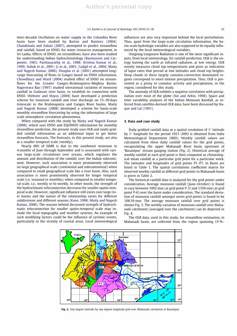
Daily gridded rainfall data at a spatial resolution of 1� latitudeby 1� longitude for the period 1951–2003 is obtained from IndiaMeteorological Department (IMD). Weekly rainfall values arecalculated from these daily rainfall values for the grid points,encapsulating the upper Mahanadi River basin upstream of‘Basantpur’ stream gauging station (Fig. 2). Historical average ofweekly rainfall at each grid point is then computed as climatolog-ical mean rainfall at a particular grid point for a particular week.The latitudes and longitudes of grid points P1–P7, in Basin arelisted in Table 1. The spatial correlations coefficient matrix forobserved weekly rainfall at different grid points in Mahanadi basinis given in Table 2.

The historical rainfall data is analyzed for the grid points underconsideration. Average monsoon rainfall (June–October) is foundto vary between 1092 mm (at grid point P-3) and 1358 mm (at gridpoint P-6) over the basin under consideration. The standard devia-tion of monsoon rainfall amongst seven grid points is found to be108.59 mm. The average monsoon rainfall over grid points isshown Fig. 3. The weekly variation of monsoon rainfall over Maha-nadi catchment (averaged over the catchment) can be depicted inFig. 4.

The OLR data, used in this study, for streamflow estimation, inMahanadi basin, are collected from the region spanning 15�N–

Fig. 2. One degree latitude by one degree longitude grid over Mahanadi catchment at Basantpur.

S.S. Kashid et al. / Journal of Hydrology 395 (2010) 23–38 25


25�N and 75�E–90�E at 2.5� latitude and longitude intervals. Thedaily mean values of OLR over this region, for 15 years, from 1stJanuary 1990 to 31st December 2004, are used in this study. Theextensions, beyond the catchment, are deliberately taken to cap-ture the effect of advancing cloud systems across the basin, overa period of time. The daily mean OLR data are used to deriveweekly means. The weekly mean OLR for specified region is ob-tained by summing the weekly grid values in a region and thendividing the sum by the number of grid points comprising the re-gion. The OLR anomalies for the region under consideration werethen computed by deducting average weekly OLR over the regionfrom observed OLR value for the particular week. InterpolatedOLR data used in this study was obtained from the NOAA web site(http://www.cdc.noaa.gov).

4. Multi-site weekly rainfall prediction methodology

It is mathematically difficult to use climate signals for the pre-diction of basin-scale hydrologic variables due to the inherentcomplexity of the climate systems. But such complex systemscan be modeled by using the modern Artificial Intelligence (AI)tools, like Artificial Neural Networks (ANN), Genetic Algorithm(GA)-based evolutionary optimizer and Genetic Programming

(GP). Applications of ANN may be found in wide range of hydro-logic studies, viz., rainfall–runoff modeling (Hsu et al., 1995; Minnsand Hall, 1996), synthetic inflow generation (Raman and Sunilku-mar, 1995), river flow forecasting (Dawson and Wilby, 1998; Lionget al., 2001), regional annual runoff forecasting using indices oflow-frequency climatic variability (Coulibaly et al., 2000). Ozelkanand Duckstein (2001) used Fuzzy Logic (FL) based method to dealwith parameter-uncertainties related to data and/or model struc-ture. Yu et al. (2000) combined gray and fuzzy methods for rainfallforecasting. Xiong et al. (2001) used Fuzzy Logic in flood forecast-ing, and recommended it, as an efficient system, for flood forecast-ing. GA was also used in different fields of water resourcesengineering, e.g., rainfall–runoff modeling (Wang, 1991; Savicet al., 1999; Cheng et al., 2002), water quality models (Chau,2002), operation of multi-reservoirs systems (Olivera and Loucks,1997), optimal reservoir operation (Wardlaw and Sharif, 1999).

GP is a modified form of GA, applied to population of algebraicfunctions. GA usually operates on (coded) strings of numbers,whereas GP operates on set of algebraic functions. GP results in aregression equation, relating predictors and predictands, consider-ing all possible combinations of algebraic operators. Koza (1992)defines GP as a domain-independent problem-solving approach,in which computer programs are evolved to solve, or approxi-mately solved, based on the Darwinian principles of reproductionand ‘survival of the fittest’.

The search procedure of a model deals with number of permu-tations and combinations of variables and functions in a proposedmodel. Any mathematical model can be represented by a treestructure. There exists a clean hierarchical structure, instead of aflat, one-dimensional string. The structure is made up of severalfunctions that can be easily encoded using a high-level language.Any complex, nonlinear model structure can also be representedin a similar way. The genetic operators (crossover, mutation andreproduction) are performed on these trees.

It might be interesting to compare GP with the traditional ap-proaches, such as, Autoregressive (AR) models and Neural Network(NN) approaches. ANNs do have many attractive features, but theysuffer from some limitations. The difficulty in choosing the optimalnetwork architecture and black-box nature, are the issues of con-cern to many researchers. In autoregressive model, only endoge-nous properties of the time series are used. To incorporate theexternal forcing, option of autoregressive model with exogenousinputs (ARX) may be selected. However, if the exogenous inputsare more, the computational complexity is a vital issue. In addition,it is linear in nature, which may not be suitable for many applica-tions related to hydroclimatological system. On the other hand, GPhas the unique feature, that it does not assume any functional formof the solution. It can optimize both the structure of the model and

Table 1Latitude and longitude grid points and representative geographical areas overMahanadi catchment (refer Fig. 2).

Pt. No. North latitude (degree) East longitude (degree)

P1 20.5 81.5P2 20.5 82.5P3 21.5 81.5P4 21.5 82.5P5 22.5 81.5P6 22.5 82.5P7 23.5 82.5

Table 2Correlations coefficient matrix for observed weekly rainfall at different grid points inMahanadi basin.

Grid point P-1 P-2 P-3 P-4 P-5 P-6 P-7

P-1 1.00 0.83 0.68 0.64 0.55 0.44 0.45P-2 0.83 1.00 0.72 0.73 0.57 0.49 0.49P-3 0.68 0.72 1.00 0.76 0.65 0.56 0.57P-4 0.64 0.73 0.76 1.00 0.71 0.68 0.68P-5 0.55 0.57 0.65 0.71 1.00 0.76 0.84P-6 0.44 0.49 0.56 1.00 0.76 1.00 0.87P-7 0.45 0.49 0.57 0.68 0.84 0.87 1.00

Correlation coefficients for observed weekly rainfall at different grid points.

0200400600800

1000120014001600

P-1 P-2 P-3 P-4 P-5 P-6 P-7

Grid Point

Rai

nfal

l (m

m)

Avg. Monsoon Rainfall

Fig. 3. Averaged monsoon rainfall over grid points (averaged for period 1951–2006).

0102030405060708090

100

1 3 5 7 9 11 13 15 17 19 21

Monsoon Week

Rain

fall

(mm

)

Observed Rainfall

Fig. 4. Weekly monsoon rainfall over catchment (averaged over seven grid pointsfor period 1951–2006 over basin).



its parameters. GP evolves an equation relating the output and in-put variables. Hence, it has the advantage of providing inherentfunctional relationship explicitly over techniques, such as ANN.The specialty of GP approach lies with its automatic ability to se-lect input variables that contribute beneficially to the model andto disregard those that do not (Jayawardena et al., 2005). However,GP also has disadvantages. First, GP is a computer-intensive meth-od and requires extensive computing power. However, owing toadvent of fast computing facilities available in present days, thisdisadvantage can be tackled. In GP, ‘possibly suitable’ programsare many. This may create a dubious attitude, as it seems to be dif-ficult to select the best (single) program. However, if it is agreedthat there could be many possible line of attack to address a prob-lem, having more than one ‘possible program’ would not be a skep-tical issue.

This study attempts to predict weekly rainfall at individual gridpoints based on the lagged weekly ENSO indices, lagged weeklyEQUINOO indices, rainfall at grid point at immediate previous timestep, rainfall at highest correlated grid point at previous time stepand previous time step OLR over the river basin.

4.1. Selection of predictors – details of correlations

It is necessary to decide exact number of weekly lags, for previ-ous step information of ENSO indices, EQUINOO indices and rainfall,to be included in regression. Pearson’s correlation coefficients arecalculated between the ENSO indices and average of gridded rain-fall over the basin as well as EQUINOO indices and average of grid-ded rainfall over the basin. The aforementioned correlations arealso calculated in terms of Kendall’s tau with presumption thatthe predictor–predictand relationship may not be linear.

The significance of these C.C. values was tested by calculating p-values of the correlations. The significance (both one-tailed andtwo-tailed probability values) of a Pearson correlation coefficientr, for given correlation value and the sample size are listed in theTable 3.

Pearson’s correlation coefficients are also computed betweenthe lagged and current weekly EQUINOO indices and rainfall. Thesignificance of these C.C. values was tested by calculating p-valuesof the correlations. The significance (both one-tailed and two-tailed probability values) of a Pearson correlation coefficient r,for given correlation value and the sample size are listed in Table 4.

It is observed that the both one-tailed and two-tailed probabil-ity values for EN (t-10)–EN (t-1) are significant. Also, CC values,corresponding to EN (t-7)–EN (t-1), are also significant. Hence,these inputs are used for rainfall prediction as well as for stream-flow prediction in this study.

It is observed from Figs. 5a and 5b that ENSO indices from (t-10)to (t-1) are significantly correlated with rainfall. Similarly it is

observed from Figs. 5c and 5d that EQUINOO indices from (t-7)to (t-1) are significantly correlated with rainfall. Hence, theselagged indices are used for rainfall prediction. Similarly correla-tions are also computed between present rainfall and lagged rain-fall (at same grid and nearby grid points). The correlations arefound to be significant for lag-1 (Fig. 6). Hence, gridded rainfallat lag-1, for the same grid point and neighboring grid points, areused in rainfall prediction. The correlation values, in Figs. 5a–5d,appear to be small, in general. However, for the most complexhydroclimatic teleconnection studies, these values may be consid-ered as good.

4.2. Regression for weekly gridded rainfall estimation

The weekly rainfall at individual grid point is formulated as afunction of

(i) Weekly historical avg. rainfall for present week (averagedover 1951–2003)

(ii) ENSO indices at weekly time steps: EN (t-10)–EN (t-1), i.e.,10 values

(iii) EQUINOO indices at weekly time steps: EQ (t-7)–EQ (t-1),i.e., 7 values

(iv) OLR anomaly over river basin at time step (t-1)(v) Lag-1 Rainfall at the same grid point

(vi) Lag-1 Rainfall at nearby grid point (having highest correla-tion, among all grid points, with present rainfall, at stationunder consideration)

Thus,

Rt ¼ ffHARt; ðENt�10; ENt�9 . . . ENt�1Þ;ðEQt�7; EQ t�6 . . . EQ t�1Þ;OLRt�1;Rt�1;Rnt�1g ð2Þ

Table 3p-Values indicating the significance of a Pearson correlation coefficient r between ENSO indices and predicted current week rainfall.

No ENSO time step (week) Pearson’s correlation coefficientwith current week rainfall

Probability two tailed Probability one tailed Remark regarding selectionof variable for prediction

1 EN (t-12) -0.0128 0.8370 0.4185 Not selected2 EN (t-11) 0.0042 0.9471 0.4735 Not selected3 EN (t-10) 0.0131 0.8360 0.4180 Selected4 EN (t-9) 0.0407 0.5201 0.2600 Selected5 EN (t-8) 0.0715 0.2580 0.1290 Selected6 EN (t-7) 0.0684 0.2790 0.1395 Selected7 EN (t-6) 0.0726 0.2500 0.1250 Selected8 EN (t-5) 0.0794 0.2090 0.1045 Selected9 EN (t-4) 0.0758 0.2300 0.1150 Selected10 EN (t-3) 0.0814 0.1970 0.0985 Selected11 EN (t-2) 0.0691 0.2740 0.1370 Selected12 EN (t-1) 0.0490 0.4380 0.2190 Selected

Table 4p-Values indicating the significance of a Pearson correlation coefficient r betweenEQUINOO indices and predicted current week rainfall.

No. EQUINOOtime step(week)

Pearson’scorrelationcoefficientwith currentweek rainfall

Probabilitytwo tailed

Probabilityone tailed

Remarkregardingselection ofvariable forprediction

1 EQ (t-8) �0.0269 0.669 0.334 Not selected2 EQ (t-7) 0.0804 0.203 0.102 Selected3 EQ (t-6) 0.1223 0.052 0.026 Selected4 EQ (t-5) 0.1206 0.056 0.028 Selected5 EQ (t-4) 0.1553 0.014 0.007 Selected6 EQ (t-3) 0.1499 0.017 0.009 Selected7 EQ (t-2) 0.1456 0.021 0.010 Selected8 EQ (t-1) 0.1275 0.043 0.022 Selected



where HAR denotes historical weekly average Rainfall, EN stands forENSO index, EQ stands for EQUINOO Index, OLR stands for OutgoingLongwave Radiation anomaly, R stands for weekly rainfall, Rnstands for rainfall at nearby grid point and t, t-1, t-2, etc. stand forweekly time steps.

The difference between the number of lags for ENSO and EQUI-NOO, considered in this formulation, can be justified as following.Earlier studies indicate that the effect of EQUINOO is more imme-diate than the effects of ENSO on Indian hydrologic phenomena(Maity and Nagesh Kumar, 2006). This is also convincing in the

perspective of the geographical locations. As the effect of ENSO isconsidered up to 10 lags (approximately two and half months),the EQUINOO is considered up to lag of 7 weeks.

The data consisting of Historical average weekly rainfall, laggedrainfall, lagged ENSO indices, lagged EQUINOO indices and laggedOLR anomaly of the concerned periods are arranged in the tabularform, suitable for GP tool for the rainfall prediction. The models aretrained for the period 1990–1998 and tested for 1999–2003. Theanalysis is limited to monsoon rainfall and monsoon streamflowonly.

-0.02

0

0.02

0.04

0.06

0.08

0.1

EN (t-12) EN (t-11) EN (t-10) EN (t-9) EN (t-8) EN (t-7) EN (t-6) EN (t-5) EN (t-4) EN (t-3) EN (t-2) EN (t-1)

ENSO Indices

Cor

rela

tion

Coe

ffici

ent

Fig. 5a. Pearson correlation coefficient between rainfall and ENSO indices with different lags.

00.010.020.030.040.050.060.070.080.09

0.1

EN (t-12) EN (t-11) EN (t-10) EN (t-9) EN (t-8) EN (t-7) EN (t-6) EN (t-5) EN (t-4) EN (t-3) EN (t-2) EN (t-1)

ENSO Indices

Ken

dall'

s Ta

u

Fig. 5b. Kendall’s tau between rainfall and ENSO indices with different lags.

-0.04

-0.020

0.02

0.04

0.060.08

0.1

0.12

0.140.16

0.18

EQ (t-8) EQ (t-7) EQ (t-6) EQ (t-5) EQ (t-4) EQ (t-3) EQ (t-2) EQ (t-1)

EQUINOO Indices

Cor

rela

tion

Coe

ffici

ent

Fig. 5c. Pearson’s correlation coefficient between rainfall and EQUINOO indices with different lags.



4.3. Genetic Programming

It is mathematically challenging to use climate signals for theprediction of basin-scale hydrologic variables, due to the inherentcomplexity in the climate systems. The difficulties, in modelingsuch complex systems, can be considerably reduced by using themodern ‘Artificial Intelligence’ (AI) tools. AI tools are tried nowa-days for modeling complex systems. GP is basically a GA-basedmethod, applied to a population of computer programs. While, aGA usually operates on (coded) strings of numbers, a GP operateson computer programs. The GP is similar to genetic algorithm (orrather a part of it) but unlike the later, its solution is a computerprogram or an equation, as against a set of numbers in GA.

GP has a unique feature, that it does not assume any functionalform of the solution. It can optimize both the structure of the mod-el and its parameters. GP evolves a computer program, represent-ing the model, relating the output to the input variables. Hence, ithas the advantage of providing inherent functional relationship,explicitly over other techniques, such as, ANN. The specialty ofGP approach lies with its automatic ability to select input variablesthat contribute beneficially to the model and to disregard thosethat do not. A thorough discussion of all these concepts is coveredin Koza (1992).

Application of GP needs five major preparatory steps (Koza,1992). These five steps are (i) to select the set of terminals, (ii) toselect the set of primitive functions, (iii) to decide the fitness mea-sure, (iv) to decide parameters for controlling the run and (v) to de-fine the method for designating the results and the criterion forterminating a run. These steps are shown in Fig. A1 – AppendixA. The choice of input variables is generally based on a prioriknowledge of causal variables and physical insight into the prob-

lem being studied. If the relationship, to be modeled, is not wellunderstood, then analytical techniques can be used. The aim ofGP is to evolve a function that relates the input information tothe output information, which is of the form:

Y ¼ f ðXnÞ ð3Þ

where Xn is an n-dimensional input vector and Y is an output vector.In all the results reported here, Linear Genetic Programming (LGP)approach is used for formulating rainfall and streamflow-predictionmodels. The GP software ‘Discipulus’, developed by Francone(1998), Machine Learning Technologies Inc., Littleton, CO., USA, isused as a GP tool in this study. This GP tool evolves ‘functions’ incomputer language ‘C’, connecting the inputs to the target output,using data sets of the input variables and output, during the ‘train-ing’ process. The models are then ‘tested’ on the unseen data.

Genetic Programming tool is used for water resources problemsby many researchers. Whigham and Crapper (2001) used GeneticProgramming for rainfall–runoff modeling. Liong et al. (2001) ex-plored GP as a flow forecasting tool. Muttil and Liong (2001) usedGP for improving runoff forecasting by input variable selection.Dorado et al. (2003) used ANN and GP for prediction and modelingof the rainfall–runoff transformation for a typical urban basin.Drunpob et al. (2005) applied Genetic Programming for streamflow rate prediction in a semi-arid coastal watershed. Makkeasornet al. (2008) compared Genetic Programming and neural networkmodels for short-term streamflow forecasting with global climatechange implications. Maity and Kashid (2010) used GP for short-term basin-scale streamflow forecasting using large-scale coupledatmospheric–oceanic circulation and local Outgoing LongwaveRadiation. Details of GP algorithms are presented in Appendix A.

-0.04

-0.02

0

0.02

0.04

0.06

0.08

0.1

0.12

EQ (t-8) EQ (t-7) EQ (t-6) EQ (t-5) EQ (t-4) EQ (t-3) EQ (t-2) EQ (t-1)

EQUINOO indices

Ken

dall'

s Ta

u

Fig. 5d. Kendall’s tau between rainfall and EQUINOO indices with different lags.

Correlations of current week rainfall with Lagged Rainfall - Grid Point 1

-0.05

0

0.05

0.1

0.15

0.2

321

Number of weeks Lag

Cor

rela

tion

Coe

ffici

ent

Fig. 6. Correlations of current time step point rainfall with lagged rainfall.

Fitness Measures

Function Set

Terminal Set

Parameters

Termination Criterion and Result Designation

A Computer Program

GP

Fig. A1. Five major preparatory steps for basic version of Genetic Programming.



4.4. Multi-site rainfall prediction

The flowchart for multi-site rainfall prediction (one grid point ata time) using Genetic Programming is shown in Fig. 7. The devel-

oped models are applied, and the results are discussed asfollowing.

As a representative example, the plots of observed weekly rain-fall and GP predicted weekly rainfall at grid point P1, during train-ing period (1990–1998) and testing period (1999–2003) are shownin the Figs. 8a and 8b respectively. It is observed from Fig. 8a(Training) and Fig. 8b (Testing) that the weekly rainfall can be pre-dicted with reasonable accuracy by using predictors enlisted inSection 4.2. The ENSO and EQUINOO indices, with support of OLRand lag rainfall can predict weekly rainfall with reasonable accu-racy. Correct observed rainfall data at (t-6)–(t-1) are already avail-able for streamflow prediction at the time of prediction. Thisapproach is adopted for arriving at the better streamflow forecaststhat consider the contribution of current week rainfall also (thoughpredicted) in basin-scale streamflow prediction. Thus, the stream-flow forecasts are available with one week lead time, with the pre-diction model, where rainfall (GP predicted) at current time step (t)is used.

The C.C. matrix is computed for grid point wise observed rain-fall and GP predicted rainfall for comparison. The correlation coef-ficients amongst the GP predicted rainfall at different grid pointsare reported in Table 6. Both the C.C. matrices, i.e. for observedrainfall and GP predicted rainfall do not match perfectly. It maybe considered as the limitation of the model. Such limitations formulti-site rainfall prediction are also reported by Toth et al.(2000). The limitation may be due to the fact that hydroclimatic

Lag rainfall (t-1) at highest correlated nearby

Grid Point

Lag ENSO indices (t-10) through (t-1)

Genetic Programming

Tool

Lag EQUINOO indices (t-7) through (t-1)

Lag OLR (t-1) over basin

Lag rainfall (t-1) at particular Grid Point

Multi-gridded

rainfall at current weekly

time step (t)

Historical Weekly Avg. rainfall of current week

Fig. 7. Flowchart of multi-gridded rainfall prediction followed by basin-scalestreamflow prediction using Genetic Programming.

r-square = 0.677

0

50

100

150

200

250

300

350

400

1990 1991 1992 1993 1994 1995 1996 1997 1998

Monsoon Weeks of Year

Rai

nfal

l (m

m)

ObservedPredicted

Fig. 8a. Observed and GP predicted weekly rainfall over Mahanadi basin for grid point P1 (Training).

ObservedPredicted

r-square= 0.363

0

50

100

150

200

250

300

350

400

1999 2000 2001 2002 2003


Rai

nfal

l (m

m)

Fig. 8b. Observed and GP predicted weekly rainfall over Mahanadi basin for grid point P1 (Testing).



teleconnection is prominently experienced over large spatial scale(e.g. continental). Hence, the models are unable to reproduce spa-tial correlation satisfactorily.

Rainfall prediction models are developed for all seven gridpoints in the Mahanadi catchment. The performance of the modelsis assessed by calculating the Pearson’s correlation coefficients be-tween observed and computed rainfall.

The ‘Nash–Sutcliffe model efficiency coefficient’ is also used toassess the predictive power of rainfall prediction. It is defined as:

E ¼ 1�PT

t¼1 Q to � Q t

m

� �2

PTt¼1 Q t

o � Q o

� �2 ð4Þ

where Qo is observed rainfall and Qm is modeled value of rainfall. Qto

is observed value of rainfall at time t and Q is mean rainfall. Nash–Sutcliffe efficiencies can range from �1 to 1. An efficiency of 1(E = 1) corresponds to a perfect match of modeled discharge tothe observed data. An efficiency of 0 (E = 0) indicates that the modelpredictions are as accurate as the mean of the observed data,whereas an efficiency less than zero (E < 0) occurs when the ob-served mean is a better predictor than the model. Essentially, thecloser the model efficiency is to 1, the more accurate the modelis. The performances of the seven rainfall prediction models interms of Pearson’s correlation coefficient and Nash–Sutcliffe coeffi-cient are listed in Table 5.

Simultaneous rainfall prediction at all seven grid points is triedfirstly using Artificial Neural Networks. But the results are not sat-isfactory due to too many complexities in atmospheric systemsand large distances between the grid points. Also, one cannot ex-pect same meteorological conditions over the extensive catchmentarea over 40,000 km2. Hence, weekly rainfall prediction models aredeveloped for every individual grid point separately, as discussedin Section 4.2.

The adopted Genetic Programming approach is compared withArtificial Neural Networks (ANN) and Linear Regression (LR) interms of correlation coefficients between observed and predictedstreamflow. Two layer Artificial Neural Network is chosen with‘Nguyrn-Wirdow’ layer initializations function. The hyperbolic tan-gent sigmoid transfer function is used as the transfer function in

the first layer. Linear transfer function is used in the second layerto calculate a layer’s output from its net input. The network train-ing function updates weights and bias values according to the resil-ient back propagation algorithm. The error performance is assessedwith the Mean Squared Error (MSE) function. Table 7 presentscomparative results amongst these three approaches. It is observedfrom Table 7 that the Genetic Programming approach gives betterresults when compared to Artificial Neural Networks and LinearRegression during testing phase. This underlines the efficacy of Ge-netic Programming in modeling such a complex system.

4.5. Rainfall forecasting by excluding ENSO, EQUINOO and OLRinformation

The novelty of this study lies in the use of large scale atmo-spheric circulation pattern information (ENSO and EQUINOO) aswell as Outgoing Longwave Radiation (OLR) for weekly rainfall pre-diction. The superiority of the model is demonstrated by compar-ing the models which use ENSO, EQUINOO and OLR informationwith those which do not use the ENSO, EQUINOO and OLR informa-tion. Table 8 compares the r2 values during training and testing, for

Table 6Correlations coefficient matrix for GP predicted weekly rainfall at different grid pointsin Mahanadi basin.

Grid point P-1 P-2 P-3 P-4 P-5 P-6 P-7

P-1 1.000 0.803 0.749 0.608 0.643 0.589 0.555P-2 0.803 1.000 0.688 0.568 0.655 0.584 0.556P-3 0.749 0.688 1.000 0.654 0.726 0.694 0.636P-4 0.608 0.568 0.654 1.000 0.579 0.672 0.631P-5 0.643 0.655 0.726 0.579 1.000 0.740 0.682P-6 0.589 0.584 0.694 0.672 0.740 1.000 0.753P-7 0.555 0.556 0.636 0.631 0.682 0.753 1.000

Correlation coefficients for GP predicted weekly rainfall at different stations.

Table 5The Pearson’s correlation coefficients and Nash–Sutcliffe coefficient between observed and predicted rainfall for seven grid points.

Gridpoint

C.C. between observed andpredicted rainfall (Training)

C.C. between observed andpredicted rainfall (Testing)

Nash–Sutcliffe coefficient betweenobserved and predicted rainfall (Training)

Nash–Sutcliffe coefficient betweenobserved and predicted rainfall (Testing)

1 0.823 0.602 0.618 0.3472 0.772 0.694 0.559 0.4433 0.682 0.579 0.450 0.3284 0.888 0.581 0.732 0.3435 0.754 0.614 0.558 0.3756 0.789 0.494 0.596 0.2337 0.822 0.607 0.669 0.366

Note: C.C: Pearson’s correlation coefficient (r).

Table 7Comparison of Pearson’s correlation coefficient values between observed andpredicted rainfall using different tools.

Grid point Pearson’s correlation coefficient

GeneticProgramming

Artificial NeuralNetworks

Linear Regression

Training Testing Training Testing Training Testing

1 0.823 0.602 0.745 0.255 0.537 0.5152 0.855 0.632 0.744 0.294 0.604 0.4883 0.682 0.579 0.743 0.208 0.611 0.5614 0.888 0.581 0.729 0.238 0.689 0.5145 0.754 0.614 0.786 0.304 0.645 0.6116 0.789 0.494 0.719 0.203 0.629 0.4807 0.822 0.607 0.671 0.272 0.607 0.551

Table 8Comparison of GP models which do not use the ENSO, EQUINOO and OLR information(uses average streamflow for present week) with those which use ENSO, EQUINOOand OLR information.

Grid point Analysis without using ENSOEQUINOO and OLR information

Analysis by using ENSO,EQUINOO and OLRinformation

r2 (Training) r2 (Testing) r2 (Training) r2 (Testing)

1 0.522 0.333 0.677 0.3622 0.487 0.348 0.731 0.3993 0.438 0.286 0.465 0.3354 0.653 0.178 0.788 0.3375 0.469 0.322 0.569 0.3776 0.507 0.216 0.623 0.2447 0.62 0.290 0.676 0.369



the GP models, which do not use ENSO and EQUINOO information,with those, using ENSO and EQUINOO information.

It is observed from results (Table 8) that the r-square values be-tween observed and predicted rainfall during training and testingshow improvements, when the ENSO, EQUINOO and OLR informa-tion are used. This indicates the usefulness of global as well as localmeteorological inputs for rainfall prediction.

5. Streamflow prediction by rainfall–runoff modeling approach

Genetic Programming is used to translate the gridded rainfallinformation into streamflow. Auto-correlations are normally foundto be significant in streamflow studies. Hence, streamflow inimmediate previous time step is also considered as input in thepresent study. The basin-scale streamflow prediction is performedusing data from 1990 to 2003, among which, monsoon rainfall dataof years 1990–1998 are used for training purpose. The data from1999 to 2003 are used for testing purpose.

Three different analyses are carried out by using three alterna-tive methodologies which are described as follows.

(i) First, the rainfall–runoff models are developed for weeklystreamflow (SFt) prediction, with rainfall information as, RO

(t-6)–RO (t-1), and streamflow during immediate previousweek.

SFt ¼ ffðSFt�1Þ; ðRO1Þt�6; ðRO2Þt�6; ðRO3Þt�6; . . . ; ðRO7Þt�6Þ;ððRO1Þt�5; ðRO2Þt�5; ðRO3Þt�5; . . . ; ðRO7Þt�5Þ; . . . ððRO1Þt�1;

ðRO2Þt�1; ðRO3Þt�1; . . . ; ðRO7Þt�1Þg; ð5Þ

where SF is streamflow, RO1, RO2, . . . , RO7 are observed rain-fall values at Grid Points P-1, P-2, . . . , P7, t, t-1, t-2 , . . .,t-6are weekly time steps.

(ii) Rainfall–runoff models are developed with weekly areaweighted observed rainfall for (t-6) to (t) time steps, forstreamflow (SFt) prediction.

SFt ¼ ffðSFt�1ÞððRO1Þt�6; ðRO2Þt�6; ðRO3Þt�6; . . . ;RO7Þt�6Þ;ððRO1Þt�5; ðRO2Þt�5; ðRO3Þt�5; . . . ;RO7Þt�5Þ; . . .

ððRO1Þt ; ðRO2Þt ; ðRO3Þt; . . . ;RO7ÞtÞg; ð6Þ

(iii) Rainfall–runoff models with observed rainfall for (t-6)–(t-1)time steps and GP predicted rainfall at time step (t) [Rp(t)] forweekly streamflow prediction. Thus, the equation can bewritten as:

SFt ¼ ffðSFt�1Þ; ðRO1Þt�6; ðRO2Þt�6; ðRO3Þt�6; . . . ;RO7Þt�6Þ;ððRO1Þt�5; ðRO2Þt�5; ðRO3Þt�5; . . . ;RO7Þt�5Þ; . . . ððRP1Þt ;ðRP2Þt; ðRP3Þt; . . . ;RP7ÞtÞg; ð7Þ

The developed models are used for streamflow prediction with ob-served rainfall up to (t-1) time step and GP predicted rainfall at timestep (t). The advantages of this approach are first, it considers cur-rent step rainfall also in streamflow prediction, for better accuracy;second, the forecasts are available in one week lead time.

6. Streamflow prediction by single-step method

The problem of weekly streamflow forecasting is solved withsingle-step method, for comparison, by directly relating large-scalecirculation and local meteorological information with streamflow.

The revised model uses

(i) Lagged streamflow in immediate previous week(ii) ENSO indices at weekly time steps: (t-10)–(t-1), i.e., 10

values

(iii) EQUINOO indices at weekly time steps: (t-7)–(t-1), i.e., 7values

(iv) OLR anomaly over river basin during time step (t-1)(v) Weekly historical avg. rainfall during particular week (aver-

aged over 1951–2003)(vi) Rainfall at the same grid point in over last 6 weeks.

Thus, the weekly rainfall at individual grid point is formulatedas a function of

SFt ¼ fffSFt�1; ðENt�10; ENt�9; . . . ; ENt�1Þ; ðEQ t�7; EQt�6 . . . ; EQt�1Þ;OLRt�1g; ðHARt1;HARt2;HARt3;HARt4;HARt5;HARt6;HARt7Þ;ððRO1Þt�6; ðRO2Þt�6; ðRO3Þt�6; . . . ;RO7Þt�6Þ;ððRO1Þt�5; ðRO2Þt�5; ðRO3Þt�5; . . . ;RO7Þt�5Þ; . . . ððRO1Þt�1;

ðRO2Þt�1; ðRO3Þt�1; . . . ; ðRO7Þt�1Þg ð8Þ

where SF is streamflow, HAR stands for historical weekly averageRainfall at particular grid point (1, 2, 3, etc.), EN stands forENSO index, EQ stands for EQUINOO Index, OLR stands for Out-going Longwave Radiation anomaly, RO stands for weekly observedrainfall, and t, t-1, t-2, etc. stand for weekly time steps.RO1, RO2, . . . , RO7 are observed rainfall values at Grid PointsP1, P2, . . . , P7. t, t-1, t-2, . . . , t-6 are weekly time steps.

7. Results and Discussion

First, the performance of rainfall–runoff models, developed byusing weekly observed rainfall during weeks, (t-6)–(t-1) are evalu-ated in terms of correlation coefficient. The correlation coefficientsbetween observed streamflow and GP-predicted streamflow arecalculated. They are 0.715 during training and 0.741 during testing.(r2 = 0.514 during training and r2 = 0.555 during testing). The plotsof Observed and GP-Predicted Streamflow, using this approach,during training and testing are presented in Figs. 9a and 9brespectively.

The rainfall–runoff models, presented in Eq. (6), are then usedfor prediction of streamflow, with weekly area weighted observedrainfall for time steps (t-6)–(t) as inputs. This combination is ob-served to predict streamflows satisfactorily, which can be depictedfrom correlation coefficient of 0.931 during training and 0.817 dur-ing testing (r2 = 0.867 during training and r2 = 0.669 during test-ing). The improvement in results for approach 2 (Eq. (6)), overapproach 1 (Eq. (6)), is due to the inclusion of observed rainfallat current time step (t) for streamflow prediction. This also under-lines the utility of rainfall value at time step (t) for streamflow pre-diction. The plots of Observed and GP Predicted Streamflow, by thisapproach, during training and testing, are presented in Figs. 10aand 10b, respectively.

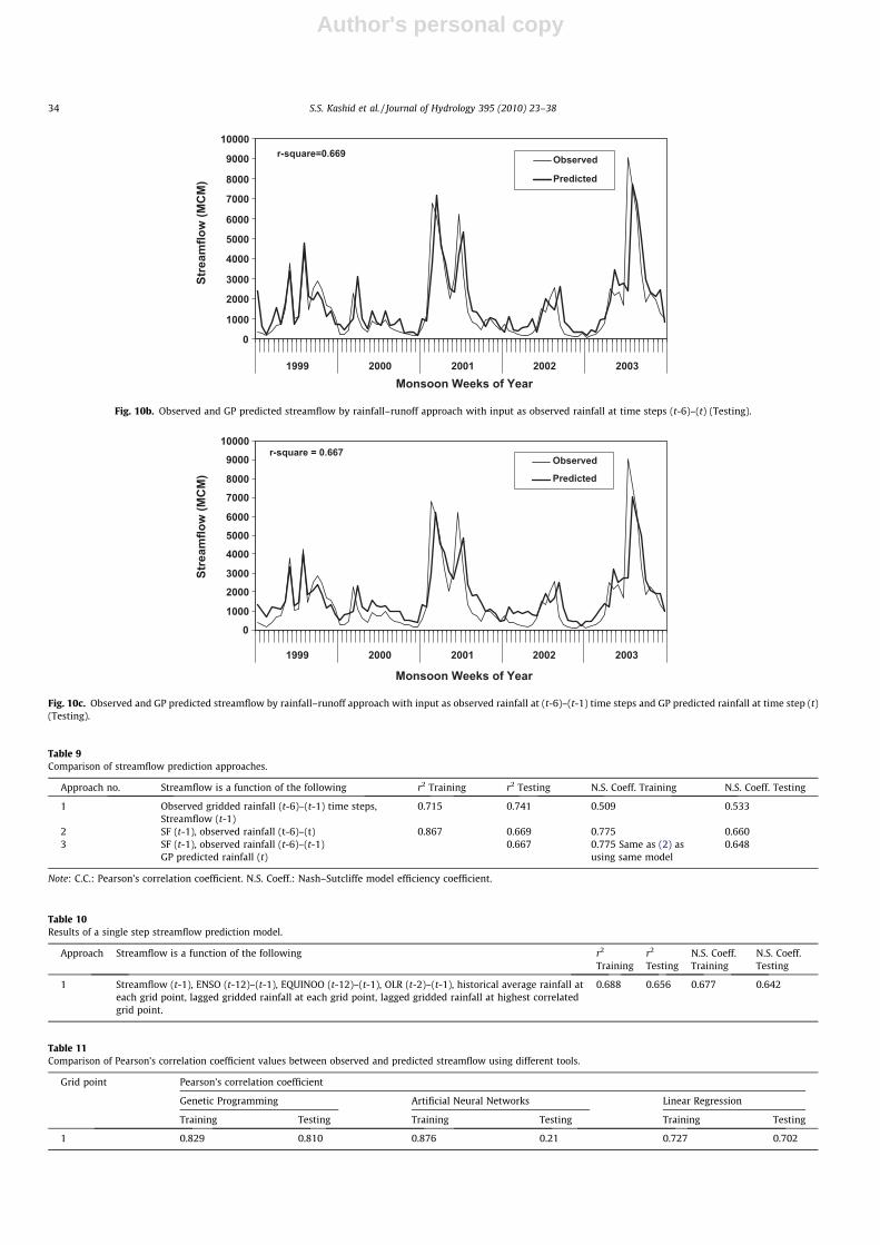
However, rainfall at present time step cannot be used in oneweek lead time. Hence, it is decided to use GP-predicted griddedrainfall values, at time step (t) in place of observed rainfall values,at present time step. In the third model (Eq. (7)), rainfall–runoffrelationship is developed, with observed rainfall from (t-6) to(t-1) and GP predicted rainfall, during time period (t). The correla-tion coefficient between observed and predicted streamflow arefound to be 0.812 (r2 = 0.667). The slight reduction, in this valuewhen compared to approach 2, may be due to the deviations ofGP-predicted rainfall, with respect to observed rainfall, at time step(t). The plots of observed and GP-predicted streamflow by thisthird approach (Eq. (7)) are presented in Fig. 10c. The predictionsare also evaluated based on the Nash–Sutcliffe model efficiencycoefficients. The performances of above three models in terms ofPearson’s correlation coefficients and Nash–Sutcliffe model effi-ciency coefficients are tabulated in Table 9.



Thus, it can be concluded that the two-step methodology ofweekly streamflow prediction, with historical average rainfall ofcurrent time step, observed rainfall up to (t-1) time step and GPpredicted rainfall at current time step (based on ENSO, EQUINOO

and Lag-1 rainfall at grid point and Lag-1 OLR), gives reasonablyaccurate basin-scale streamflow forecasts, with 1 week lead time.The forecasts can be certainly useful for basin-scale real time watermanagement. Similar models can be developed for basin-scale

r-square = 0.511

0

2000

4000

6000

8000

10000

12000

14000

16000

1990 1991 1992 1993 1994 1995 1996 1997 1998


Stre

amflo

w (M

CM

)

ObservedPredicted

Fig. 9a. Observed and GP predicted streamflow by rainfall–runoff approach with input as observed rainfall at (t-6)–(t-1) time steps (Training).

r-square = 0.555

0

1000

2000

3000

4000

5000

6000

7000

8000

9000

10000

1999 2000 2001 2002 2003


Stre

amflo

w (M

CM

)

ObservedPredicted

Fig. 9b. Observed and GP predicted streamflow by rainfall–runoff approach with input as observed rainfall at (t-6)–(t-1) time steps (Testing).

r-square = 0.867

0

2000

4000

6000

8000

10000

12000

14000

16000

1990 1991 1992 1993 1994 1995 1996 1997 1998

Monsoon Weeks

Stre

amflo

w (M

CM

)

ObservedPredicted

Fig. 10a. Observed and GP predicted streamflow by rainfall–runoff approach with input as observed rainfall at time steps (t-6)–(t) (Training).



r-square=0.669

0

1000

2000

3000

4000

5000

6000

7000

8000

9000

10000

1999 2000 2001 2002 2003Monsoon Weeks of Year

Stre

amflo

w (M

CM

)

Observed

Predicted

Fig. 10b. Observed and GP predicted streamflow by rainfall–runoff approach with input as observed rainfall at time steps (t-6)–(t) (Testing).

r-square = 0.667

0

1000

2000

3000

4000

5000

6000

7000

8000

9000

10000

1999 2000 2001 2002 2003


Stre

amflo

w (M

CM

)

Observed

Predicted

Fig. 10c. Observed and GP predicted streamflow by rainfall–runoff approach with input as observed rainfall at (t-6)–(t-1) time steps and GP predicted rainfall at time step (t)(Testing).

Table 9Comparison of streamflow prediction approaches.

Approach no. Streamflow is a function of the following r2 Training r2 Testing N.S. Coeff. Training N.S. Coeff. Testing

1 Observed gridded rainfall (t-6)–(t-1) time steps,Streamflow (t-1)

0.715 0.741 0.509 0.533

2 SF (t-1), observed rainfall (t-6)–(t) 0.867 0.669 0.775 0.6603 SF (t-1), observed rainfall (t-6)–(t-1)

GP predicted rainfall (t)0.667 0.775 Same as (2) as

using same model0.648

Note: C.C.: Pearson’s correlation coefficient. N.S. Coeff.: Nash–Sutcliffe model efficiency coefficient.

Table 10Results of a single step streamflow prediction model.

Approach Streamflow is a function of the following r2

Trainingr2

TestingN.S. Coeff.Training

N.S. Coeff.Testing

1 Streamflow (t-1), ENSO (t-12)–(t-1), EQUINOO (t-12)–(t-1), OLR (t-2)–(t-1), historical average rainfall ateach grid point, lagged gridded rainfall at each grid point, lagged gridded rainfall at highest correlatedgrid point.

0.688 0.656 0.677 0.642

Table 11Comparison of Pearson’s correlation coefficient values between observed and predicted streamflow using different tools.

Grid point Pearson’s correlation coefficient

Genetic Programming Artificial Neural Networks Linear Regression

Training Testing Training Testing Training Testing

1 0.829 0.810 0.876 0.21 0.727 0.702



streamflow prediction for other river basins, where hydroclimaticteleconnection is prominently noticed.

Results of the single-step methodology can be discussed as fol-lowing. The r2 values between observed and predicted streamflowduring training and testing are found to be 0.688 and 0.656, respec-tively, when compared to 0.867 during training and 0.669 duringtesting, for a two-step model (Refer Table 10 for GP results andTable 11 for the comparison).

It is observed that the results of single step model are inferior,for both training and testing. The results can also be compared interms of simulating peak streamflows. (Figs. 10c,11a and 11b).Though the single-step model shows comparable r2 value duringtesting of GP models, the plots of observed and predicted stream-flow for two-step model show that the peak streamflows are bettersimulated by the two-step model. This is due to the most naturalrainfall–runoff approach, adopted for streamflow prediction, inthe two-step methodology.

It is well understood from the analysis that the local meteoro-logical information over the catchment is as important as large-scale circulation pattern information for rainfall prediction. Localmeteorological information, in form of Outgoing Longwave Radia-tion (OLR), is thus, included in rainfall prediction models at all se-ven grid points.

The reasons behind using weekly ENSO index, in rainfall as wellas streamflow forecasting, is discussed here. The strength of east-erly trade winds and the amount of moisture transfer are largelyinfluenced by the sea surface temperature anomalies and associ-

ated pressure anomalies over tropical Pacific Ocean. The El NiñoSouthern Oscillation Index (ENSO index) happens to be the indica-tor of these activities observed over tropical Pacific Ocean. ‘El NiñoSouthern Oscillation’ can show three conditions viz. ‘El Niño’ con-ditions, ‘Normal’ conditions and ‘La Niña’ conditions. The stream-flow forecasting models perform well in all the times, i.e. during‘El Niño’ conditions, ‘Normal’ conditions and ‘La Niña’ conditions.Furthermore, ‘El Niño’ and ‘La Niña’ can also be ‘weak’, ‘moderate’or ‘strong’, depending upon the ‘Oceanic Niño Index’ (ONI) used byNOAA.

El Niño conditions are said to be developed when SST anomalyremains on the negative side of �0.5 over seven consecutivemonths, whereas La Niña conditions are said to be developed whenSST anomaly on positive side of +0.5 over seven consecutivemonths. The conditions in between are called as ‘Normal condi-tions’. For Indian Summer Monsoon, the sea surface temperatureanomalies from March to September are most important, as mon-soon rains extends from June to middle of October in India. It canbe interesting to know the ENSO status over the period of analysis.Accordingly the yearly ENSO conditions are listed as following:1990 – normal conditions, 1991 – strong El Niño, 1992 – normalconditions, 1993 – normal conditions, 1994 – moderate El Niño,1995 – weak La Niña, 1996 – normal conditions, 1997 – strong ElNiño, 1998 – moderate La Niña, 1999 – moderate La Niña, 2000– weak La Niña, 2001 – normal conditions, 2002 – moderate ElNiño, 2003 – normal conditions (Source: http://www.cpc.noaa.-gov/products/analysis_monitoring/ensostuff/ensoyears.shtml).

r-square=0.688

0

2000

4000

6000

8000

10000

12000

14000

16000

1990 1991 1992 1993 1994 1995 1996 1997 1998


Stre

amflo

w (M

CM

)

ObservedPredicted

Fig. 11a. Observed and GP predicted streamflow by single step approach (Training).

r-square=0.669

0100020003000400050006000700080009000

10000

1999 2000 2001 2002 2003


Stre

amflo

w (M

CM

)

ObservedPredicted

Fig. 11b. Observed and GP predicted streamflow by single step approach (Testing).



The models in this study use weekly ENSO indices of 12 imme-diate previous weeks (12 values) and EQUINOO indices of 7 imme-diate previous weeks (7 values) as inputs for weekly streamflowprediction. It should be noted here that several weeks of lags areused to incorporate evolutionary trends in the data of the inputvariables.

It is observed that lagged negative values of ENSO indices leadto below normal rainfall and streamflow. On the other hand, thelagged positive ENSO indices lead to above normal rainfall andstreamflow. The performances of model in monsoon weeks ofyears 1999, 2000, 2001, 2002 and 2003 are observed in this study.Out of 90 weekly streamflow data, in testing, it is observed that 65are correct. This shows the efficacy of ENSO index for rainfall andstreamflow prediction.

The studies by Eltahir (1996), Piechota et al. (1997) and Chiewet al. (1998) use ENSO as the principal indicator of streamflowvariation, whereas the present study includes EQUINOO fromEquatorial Indian Ocean and basin-scale OLR for rainfall andstreamflow prediction. Inclusion of EQUINOO and local meteoro-logical information (OLR) makes this study different from the ear-lier studies.

The rainfall prediction models as well as streamflow-predictionmodels, developed in this study, use large number of predictors.The selection of predictors, as well as the improvement in predic-tive skill, from each variable, in such cases can benefit from the useof nonlinear dependence measures, which are robust to noise andshort length of the data. However, this can be the future scope ofthe present study.

8. Concluding remarks

The information of large scale atmospheric circulation pat-terns viz. El Niño Southern Oscillation (ENSO) and Equatorial In-dian Ocean Oscillation (EQUINOO), with support of laggedrainfall information at every individual grid point and basin-scaleOLR anomaly are successfully used for prediction of weekly grid-ded monsoon rainfall, in Mahanadi catchment with reasonableaccuracy.

Results of this study show that the inclusion of GP-predictedrainfall, at current time step (t), as input, for weekly streamflowprediction model, gives better basin-scale streamflow forecasts,when compared to streamflow prediction based on observed grid-ded rainfall up to the last weekly, i.e. (t-1) time step.

GP-derived rainfall–runoff models that use observed griddedrainfall up to weekly time step (t-1) and GP predicted gridded rain-fall at weekly time step (t) give better streamflow forecasts thanthose models using rainfall up to (t-1) time step.

The blending large-scale circulation information in form ofENSO and EQUINOO indices, local meteorological information inform of OLR and lagged rainfall at grid points can be advantageousfor the basin-scale streamflow forecasting.

The efficacy of Genetic Programming approach can be realizedthrough experience of modeling of the most complex hydrometeo-rological systems analyzed in this study.

Appendix A. Genetic Programming approach

This appendix describes the Genetic Programming (GP) ap-proach, applied in the studies, reported in this paper. GP is basi-cally a genetic algorithm (GA) applied to a population ofcomputer programs. While a GA usually operates on (coded)strings of numbers, a GP operates on computer programs. The GPis similar to genetic algorithm (or rather a part of it) but unlikethe latter, its solution is a computer program or an equation, asagainst a set of numbers in GA. Koza (1992) defines GP as a domain

independent problem-solving approach in which computer pro-grams are evolved to solve, or approximately solve, problemsbased on the Darwinian principles of reproduction and ‘survivalof the fittest’.

Genetic Programming starts with solving a problem, by creatingmassive amount of simple random functions, in a population pool.These simple parent functions mate and reproduce massiveamount of children offspring functions. Each offspring function ismeasured against the training data. Those offspring functions thatclosely match the training data may be kept and be allowed toreproduce, while some of the poor-fitted offspring functions wouldbe terminated. The selected offspring functions, determined bytheir fitness, can reproduce another generation of grandchildrenfunctions. Each grandchildren function may be tested against thetraining input data for its fitness. The good-fitted grandchildrenfunctions may be kept and used to reproduce the next generation.Some low-fitting grandchildren functions may be terminated. Thispopulation of functions is progressively evolved over a series ofgenerations. The search for the best result in the evolutionary pro-cess involves applying the principle of survival of the fittest. The GPcan reproduce and terminate millions of function over thousandsof generations to find the strongest function that fits the traininginput data the most. Regression models generated from the GPare free from any particular model structure (Chang and Chen,2000).

The glass box characteristic of GP reveals structures of theregression models, which is the significant advantage of the GPover black box approaches such as neural networks. The GP modelcould be the best solver for searching highly nonlinear spaces forglobal optima via adaptive strategies.

The three important operators used in GP are crossover, repro-duction, and mutation. These can be described in brief which are asfollows. According to Koza (1992), the operator ‘crossover’ ismainly responsible for the genetic diversity in the population ofprograms. Similar to GA, crossover (a binary operator) operateson two programs in GP and produces two child programs. Thesenew programs become part of the next generation of programsto be evaluated. The operation ‘Reproduction’ is performed by sim-ply copying a selected member from the current generation to thenext generation. Mutation becomes an important operator in ge-netic algorithms, which provides diversity to the population. How-ever, as per Koza (1992), mutation is relatively unimportant in theGenetic Programming, because the dynamic sizes and shapes of theindividuals in the population already provide diversity. Mutationcan be rather considered as a variation on the crossover operationin GP. The flowchart of Genetic Programming methodology isshown in Fig. A2.

Application of GP needs five major preparatory steps (Koza,1992). These five steps are (i) to select the set of terminals, (ii) toselect the set of primitive functions, (iii) to decide the fitness mea-sure, (iv) to decide parameters for controlling the run, and (v) todefine the method for designating the results and the criterionfor terminating a run. A flow chart showing five major preparatorysteps involved in basic version of GP is shown in Fig. A1. The choiceof input variables is generally based on a priori knowledge of ca-sual variables and physical insight into the problem being studied.If the relationship to be modeled is not well understood, then ana-lytical techniques can be used. The aim of GP is to evolve a functionthat relates the input information to the output information, whichis of the form:

Ym ¼ f ðXnÞ ð9Þ

Where Xn, an n-dimensional input, is vector, and Ym is an m-dimen-sional output vector. For example, for the weekly streamflow pre-diction problem, the input vector may consist of lag streamflow



(of previous week), lagged ENSO and EQUINOO indices of certainnumber weeks and OLR anomaly of previous week. The outputcan be of streamflow at current weekly time step.

The implementation of GP in this work is done through soft-ware Discipulus (Francone, 1998) that is based on an extensionof the originally envisaged GP called Linear Genetic Programming

(LGP). It evolves sequences of instructions from an imperative pro-gramming language or machine language. The LGP expressesinstructions in a line-by-line mode. The term ‘‘linear’’ in Linear Ge-netic Programming refers to the structure of the (imperative) pro-gram representation. It does not stand for functional geneticprograms that are restricted to a linear list of nodes only. Genetic

Fig. A2. Flowchart for Genetic Programming (Hong and Bhamidimarri, 2003).



programs normally represent highly nonlinear solutions in thismeaning (Brameier, 2004).

References

Ashok, K., Guan, Z., Yamagata, T., 2001. Impact of Indian Ocean dipole on therelationship between the Indian monsoon rainfall and ENSO. GeophysicsResearch Letters 28, 4499–4502.

Ashok, K., Guan, Z., Saji, N., Yamagata, T., 2004. Individual and combined effect ofENSO and Indian Ocean dipole on the Indian summer monsoon. Journal ofClimate 17 (16), 3141–3155. doi:10.1175/1520-0442(2004)017<3141:IACIOE>2.0.CO;2.

Barton, S.B., Ramirez, J.A., 2004. Effects of El Niño Southern Oscillation and PacificInterdecadal Oscillation on water supply in the Columbia River basin. Journal ofWater Resources Planning and Management 130 (4), 281–289.

Brameier, M., 2004. On Linear Genetic Programming. PhD Thesis, FachbereichInformatik, Universit’’at Dortmund, Germany.

Cane, M.A., 1992. Tropical Pacific ENSO Models: ENSO as a mode of couples system.In: Trenberth, K.E. (Ed.), Climate System Modeling. Cambridge University Press,UK.

Chandimala, J., Zubair, L., 2007. Predictability of stream flow and rainfall based onENSO for water resources management in Sri Lanka. Journal of Hydrology 335,303–312.

Chang, N.B., Chen, W.C., 2000. Prediction of PCDDs/PCDFs emissions from municipalincinerators by genetic programming and neural network modeling. WasteManagement & Research 18, 341–351.

Chau, K.W., 2002. Calibration of flow and water quality modeling using geneticalgorithms. Lecture Notes in Artificial Intelligence 2557, 720.

Cheng, C.T., Ou, C.P., Chau, K.W., 2002. Combining a fuzzy optimal model with agenetic algorithm to solve multi-objective rainfall–runoff model calibration.Journal of Hydrology 268 (3), 72–86.

Chiew, F.H.S., Piechota, T.C., Dracup, J.A., McMahon, T.A., 1998. El Niño/SouthernOscillation and Australian rainfall, streamflow and drought: links and potentialfor forecasting. Journal of Hydrology 204, 138–149.

Chowdhury, M.R., Ward, N., 2004. Hydro-metrological variability in the greaterGanges–Brahmaputra–Meghna basins. International Journal of Climatology 24,1495–1508.

Coulibaly, P., Anctil, F.F., Rasmussen, P., Bobee, B., 2000. A recurrent neural networksapproach using indices of low-frequency climatic variability to forecast regionalannual runoff. Hydrological Processes 14, 2755–2777.

Dawson, C.W., Wilby, R., 1998. An artificial neural network approach to rainfall–runoff modeling. Hydrological Sciences Journal 43 (1), 47–66.

Dorado, J., Rabunal, J.R., Pazos, A., Rivero, D., Santos, A., Puertas, J., 2003. Predictionand modelling of the rainfall–runoff transformation of a typical urban basinusing ANN and GP. Applied Artificial Intelligence 17, 329–343.

Douglas, W.W., Wasimi, S.A., Islam, S., 2001. The El Niño Southern Oscillation andlong-range forecasting of flows in Ganges. International Journal of Climatology21, 77–87.

Dracup, J.A., Kahya, E., 1994. The relat0069onship between US streamflow and LaNiña events. Water Resources Research 30 (7), 2133–2141.

Drunpob, A., Chang, N.B., Beaman M., 2005. Stream flow rate prediction usinggenetic programming model in a semi-arid coastal watershed. In: Proceedingsof EWRI 2005, ASCE.

Eltahir, E.A.B., 1996. El Niño and the natural variability in the flow of the Nile River.Water Resources Research 32 (I), 131–137.

Francone, F.D., 1998. Discipulus Owner’s Manual. Machine Learning Technologies,Inc., Littleton, Colorado.

Gadgil, S., Vinayachandran, P.N., Francis, P.A., 2003. Droughts of the Indian summermonsoon: role of clouds over the Indian Ocean. Current Science 85 (2), 1713–1719.

Gadgil, S., Vinayachandran, P.N., Francis, P.A., Gadgil, S., 2004. Extremes of theIndian summer monsoon rainfall. ENSO and equatorial Indian Ocean Oscillation.Geographical Research Letter 31, L12213. doi:10.1029/2004GLO19733.

Haque, M.A., Lal, M., 1991. Space and time variability analyses of the Indianmonsoon rainfall as inferred from satellite-derived OLR data. Climate Research1, 187–197.

Hong, Y.S., Bhamidimarri, R., 2003. Evolutionary self-organising modelling of amunicipal wastewater treatment plant. Water Research 37, 1199–1212.doi:10.1016/S0043-1354(02)00493-1.

Hsu, K.L., Gupta, H.V., Sorooshian, S., 1995. Artificial neural network modeling of therainfall–runoff process. Water Resources Research 31 (10), 2517–2530.

Jain, S., Lall, U., 2001. Floods in a changing climate: does the past represent thefuture? Water Resources Research 37 (12), 3193–3205.

Jayawardena, A.W., Muttil, N., Fernando, T.M.K.G., 2005. Rainfall–Runoff ModelingUsing Genetic Programming. <http://mssanz.org.au>.

Kane, R.P., 1998. Extremes of the ENSO phenomenon and Indian summer monsoonrainfall. International Journal of Climatology 18, 775–791.

Koza, J.R., 1992. Genetic Programming: On the Programming of Computers byMeans of Natural Selection. MIT Press, Cambridge, MA, USA.

Krishna Kumar, K., Rajagopalan, B., Cane, M.A., 1999. On the weakening relationshipbetween the Indian Monsoon and ENSO. Science 284 (5423), 2156–2159.doi:10.1126/science.284.5423.2156.

Li, T., Zhang, Y.S., Chang, C.P., Wang, B., 2001. On the relationship between IndianOcean sea surface temperature and Asian summer monsoon. GeophysicalResearch Letters 28, 2843–2846.

Liong, S.Y., Nguyen, V.T., Gautam, T.R., Wee, L., 2001. Alternative well calibratedrainfall–runoff model: genetic programming scheme. In: Paper Presented atWorld Water and Environmental Resources Congress 2001, Orlando, Florida,USA, pp. 777–787. doi:10.1061/40583(275)73.

Maity, R., Kashid, S.S., 2010. Short-term basin-scale streamflow forecasting usinglarge-scale coupled atmospheric–oceanic circulation and local outgoinglongwave radiation. Journal of Hydrometeorology 11 (2), 370–387.

Maity, R., Nagesh Kumar, D., 2006. Bayesian dynamic modeling for monthly Indiansummer monsoon rainfall using ENSO and EQUINOO. Journal of GeophysicalResearch III, D07104. doi:10.1029/2005JD006539.

Maity, R., Nagesh Kumar, D., 2007. Hydroclimatic teleconnection between globalsea surface temperature and rainfall over India at subdivisional monthly scale.Hydrological Processes 21, 1802–1813. doi:10.1002/hyp.6300.

Maity, R., Nagesh Kumar, D., 2008. Basin-scale streamflow forecasting using theinformation of large-scale atmospheric circulation phenomena. HydrologicalProcesses 22, 643–650. doi:10.1002/hyp.

Makkeasorn, A., Chang, N.B., Zhou, X., 2008. Short-term streamflow forecasting withglobal climate change implications – a comparative study between geneticprogramming and neural network models. Journal of Hydrology 352, 336–354.

Marcella, M.P., Eltahir, E.A.B., 2008. The hydroclimatology of Kuwait: explaining thevariability of rainfall at seasonal and interannual time scales. Journal ofHydrometeorology 9, 1095–1105.

Minns, A.W., Hall, M.J., 1996. Artificial neural networks as rainfall–runoff models.Hydrological Sciences Journal 41 (3), 399–418.

Muttil, N., Liong, S.Y., 2001. Improving runoff forecasting by input variable selectionin genetic programming. In: ASCE World Water Congress, vol. 111, Orlando,Florida, USA, 20–24 May, pp. 76–76. doi:10.1061/40569(2001)76.

Nageswara Rao, G., 1997. Interannual variation of monsoon rainfall in GodavariRiver basin – connections with the Southern Oscillation. Journal of Climate 11,768–771.

Olivera, R., Loucks, D.P., 1997. Operating rules for multireservoir systems. WaterResources Research 33 (4), 839–852.

Ozelkan, E.C., Duckstein, L., 2001. Fuzzy conceptual rainfall–runoff models. Journalof Hydrology 253 (1–4), 41–68.

Parthasarathy, B., Diaz, H.F., Eischeid, J.K., 1988. Prediction of all India summermonsoon rainfall with regional and large-scale parameters. Journal ofGeophysics Research 93 (5), 5341–5350.

Piechota, T.C., Dracup, J.A., Fovell, R.G., 1997. Western US streamflow andatmospheric circulation patterns during El Niño-Southern Oscillation. Journalof Hydrology 201, 249–271.

Raman, H., Sunilkumar, N., 1995. Multivariate modeling of water resources timeseries using artificial neural networks. Hydrological Sciences Journal 40 (2),145–163.

Rasmusson, E.M., Carpenter, T.H., 1983. The relationship between eastern equatorialPacific sea surface temperature and rainfall over India and Sri Lanka. MonthlyWeather Review 111, 517–528.

Saji, N.H., Goswami, B.N., Vinayachandran, P.N., Yamagata, T., 1999. A dipole modein the tropical Indian Ocean. Nature 401, 360–363.

Savic, D.A., Walters, G.A., Davidson, J.W., 1999. A genetic programming approach torainfall–runoff modeling. Water Resources Management 13, 219–231.

Toth, E., Brath, A., Montanari, A., 2000. Comparison of short term rainfall predictionmodels for real time flood forecasting. Journal of Hydrology 239 (1–4), 132–147.doi:10.1016/s0022-1694(00)00344-9.

Wang, Q.J., 1991. The genetic algorithm and its application to calibrating conceptualrainfall–runoff models. Water Resources Research 27 (9), 2467–2471.

Wardlaw, R., Sharif, M., 1999. Evaluation of genetic algorithms for optimal reservoirsystem operation. Journal of Water Resources Planning and Management, ASCE125 (1), 25–33.

Webster, P., Hoyos, C., 2004. Prediction of monsoon rainfall and river discharge on15–30 day timescale. Bulletin of American Meteorological Society. doi:10.1175/BAMS-85-11-1745.

Whigham, P.A., Crapper, P.F., 2001. Modeling rainfall–runoff using geneticprogramming. Mathematical and Computer Modeling 33, 707–721 (Canberra,Australia).

Xie, P., Arkin, P.A., 1998. Global monthly precipitation estimates from satellite-observed outgoing longwave radiation. Journal of Climate 11, 137–164.

Xiong, L., Asaad, Y., Shamseldin, Y., O’Connor, K.M., 2001. A non-linear combinationof the forecast of rainfall-runoff models by first order Takagi-Sugeno fuzzysystem. Journal of Hydrology 254 (1–4), 196–217.

Yu, P.S., Chen, C.J., Chen, S.J., 2000. Application of gray and fuzzy methods for rainfallforecasting. Journal of Hydrologic Engineering, ASCE 5 (4), 339–345.


Author's personal copy - ERNETrajibmaity/JH_Streamflow prediction...Author's personal copy Stream ow...

Documents

Transcript of Author's personal copy - ERNETrajibmaity/JH_Streamflow prediction...Author's personal copy Stream ow...