Author's personal copy -...

Author's personal copy

Locating near-surface scatterers using non-physical scattered wavesresulting from seismic interferometry

U. Harmankaya a, A. Kaslilar a,⁎, J. Thorbecke b, K. Wapenaar b, D. Draganov b

a Department of Geophysical Engineering, Faculty of Mines, Istanbul Technical University, Istanbul, Turkeyb Sec. Applied Geophysics and Petrophysics, Dept. of Geoscience and Engineering, Delft University of Technology, The Netherlands

a b s t r a c ta r t i c l e i n f o

Article history:Received 26 October 2012Accepted 11 February 2013Available online 18 February 2013

Keywords:Locating scatterers and diffractorsGhost scattered surface and body wavesActive source seismic interferometryInversionNear-surfaceFinite-difference modelling

We use controlled-source seismic interferometry (SI) and inversion in a unique way to estimate the locationof near-surface scatterers and a corner diffractor by using non-physical (ghost) scattered surface and bodywaves. The ghosts are arrivals obtained by SI due to insufficient destructive interference in the summationprocess of correlated responses from a boundary of enclosing sources. Only one source at the surface is suf-ficient to obtain the ghost scattered wavefield. We obtain ghost scattered waves for several virtual-source lo-cations. To determine the location of the scatterer, we invert the obtained ghost traveltimes by solving theinverse problem. We demonstrate the method using scattered surface waves. We perform finite-differencenumerical simulations of a near-surface scatterer starting with a very simple model and increase thecomplexity by including lateral inhomogeneity. Especially for the model with lateral variations, we showthe effectiveness of the method and demonstrate the estimation of the subsurface location of a cornerdiffractor using S-waves. In all models we obtain very good estimations of the location of the scatterer.

© 2013 Elsevier B.V. All rights reserved.

1. Introduction

The investigation and detection of near-surface structures such as cav-ities, caves, sinkholes, tunnels, mineshafts, buried objects, archeologicalruins, water reservoirs and similar is important tomitigate geo- and envi-ronmental hazards (Culshaw and Waltham, 1987). These near-surfacestructures, (henceforth called scatterers) may pose risk during and afterthe construction of buildings, transportation ways (roads, highways, rail-ways) or power plants (wind, solar, etc.), which are spread onwide areas.Furthermore, these scatterers can be affected by the changes in the hy-draulic regime, earthquakes and change of the loading on the soil andthusmay cause risk. Therefore, thedetection,monitoring and stabilizationof this type ofweak zones is important to prevent environmental and geohazards.

Especially, the detection of natural (karstic structures and caves) andman-made (tunnels,mine shafts and galleries) cavities is widely studiedin the literature. Both numerical and/or field experiments are performedfor this purpose. Several geophysical methods are available for investi-gation of the near-surface structures andeach has advantages anddisad-vantages (McCann et al., 1987). The success depends on the resolutionand penetration achieved by each method. Ground penetrating radar(GPR) (Al-fares et al., 2002; Nuzzo et al., 2007), microgravity andmulti-channel analysis of surface waves (Debeglia et al., 2006; Samynet al., 2012; Xu and Butt, 2006), seismic refraction and electric resistivity(Cardarelli et al., 2010; Nuzzo et al., 2007), seismic refraction only

(Engelsfeld et al., 2008, 2011), are some examples for the exploitedmethods that are used for detecting the cavities. Some examples of geo-logical studies on cavities and related geohazards are found in Culshawand Waltham (1987), Woodcock et al. (2006), Edmonds (2008) andKhomenko (2008).

In seismic methods, a high-accuracy subsurface image of the shal-low objects can be obtained using reflected body waves. This, though,requires high-resolution data acquired in a dense spatial array. Theseare not easily available for shallow-seismic applications. Furthermore,it might not always be possible to place active sources above the tar-get scatterer or even close enough to it. In such cases, using sourcesaway and having the generated wavefields propagate through un-known inhomogeneities might distort the results significantly. Sur-face waves are widely used in global, exploration and near-surfacegeophysics. A notable difference in the applications is the frequencycontent and the array aperture of the measurements that affect theinvestigation depth. The dispersive property of surface waves allowsthe estimation of the S-wave velocity structure and attenuation ofshallow layers. In global seismology, surface waves are used to inves-tigate the crust and upper-mantle structure (e.g. Chang and Baag,2005; Cong and Mitchell, 1998; Kovach, 1978) and the source proper-ties of seismic events (e.g. Canıtez and Toksöz, 1971; Ekström, 2006).In geotechnical engineering, S-wave velocity estimation from surfacewaves has become a popular tool and different active and passive-source techniques are applied (Bozdag and Kocaoglu, 2005; Foti,2000; Kocaoglu and Fırtana, 2011; Leparoux et al., 2000; Nazarian etal., 1983; O'Neill, 2003; Park et al., 1999; Rix et al., 1998; Socco andBoiero, 2008; Socco et al., 2009, 2010) to obtain the near-surface

Journal of Applied Geophysics 91 (2013) 66–81

⁎ Corresponding author. Tel.: +90 5334874389; fax: +90 2122856201.E-mail addresses: [email protected], [email protected] (A. Kaslilar).

0926-9851/$ – see front matter © 2013 Elsevier B.V. All rights reserved.http://dx.doi.org/10.1016/j.jappgeo.2013.02.004

Contents lists available at SciVerse ScienceDirect

Journal of Applied Geophysics

j ourna l homepage: www.e lsev ie r .com/ locate / jappgeo


properties of the medium. The surface-wave methods work underthe assumption of laterally homogeneous stratified layers. Thereforelateral inhomogeneities, such as cavities or varying overburden thick-ness and steeply dipping bedrock cause difficulties in the estimationof the velocity structure and in the evaluation of the lateral inhomo-geneities on the dispersion curve. However, Nasseri-Moghaddamet al. (2005), Bodet et al. (2010) and Boiero and Socco (2010) showthe possibility of exploiting surface-wave dispersion curves to inves-tigate voids and lateral variations of the subsurface.

Another methodology that is used for detecting the near-surfacestructures is that with scattered waves. Scattering of P-waves areused by Grandjean and Leparoux (2004), Gelis et al. (2005),Rodríguez-Castellanos et al. (2006), Mohanty (2011); coda wavesare used by Mikesell et al. (2012); and scattered surface waves areused by Snieder (1987), Herman et al. (2000), Leparoux et al.(2000), Campman et al. (2004), Grandjean and Leparoux (2004),Gelis et al. (2005), Campman and Riyanti (2007), Kaslilar (2007),Xia et al. (2007), Chai et al. (2012). Based on seismic interferometrythe scattered surface waves are studied in detail by Halliday andCurtis (2009).

We propose to use non-physical (ghost) scattered body and/or sur-face waves, obtained by seismic interferometry (SI), in an inversionscheme to estimate the location of a scatterer (Harmankaya et al.,2012a,b). The appearance of the ghost scattered waves is explainedlater in this section. SI traditionally refers to the method of retrievingthe interreceiverwavefield by cross-correlating thewavefields recordedat each of the receivers (e.g. Snieder, 2004; van Manen et al., 2006;Wapenaar, 2004; Wapenaar and Fokkema, 2006). SI can be dividedinto controlled-source and passive methods. Controlled-source SI(Schuster et al., 2004) involves cross-correlation followed by sum-mation over different controlled source positions at a boundary,while passive SI is themethodology of turning passive seismicmeasure-ments, like ambient noise and earthquakes, into impulsive seismicresponses (Draganov et al., 2007, 2009; Roux et al., 2005; Ruigroket al., 2010; Shapiro and Campillo, 2004). While SI has proven usefulin retrieving surface-wave waveforms from passive noise sources(e.g. Halliday and Curtis, 2008; Sens-Schönfelder and Wegler, 2006;Snieder andWapenaar, 2010), it is also shown that active-source signalscan be used to synthesize interreceiver surface-wave estimates, whichcan be used, for example, for predictive ground-roll removal (Donget al., 2006; Halliday et al., 2007, 2010).

To obtain the complete Green's function between the receiverswhose recorded responses we cross-correlate, the boundary sources(primary or secondary) effectively need to enclose these receivers(Wapenaar and Fokkema, 2006). When the receivers are not equallyilluminated from all directions by the boundary sources, ghost ar-rivals will appear in the SI result (Snieder et al., 2006). Furthermore,the physical arrivals might not be retrieved correctly. When using ac-tive sources at the surface, as is the standard practice for near-surfaceseismics, reflection ghosts will nearly always be present. The reflec-tion ghosts are arrivals retrieved from the correlation of two reflectedevents in the active data, whose traveltimes correspond to reflectionsas if measured with sources and receivers redatumed in the subsur-face at the levels of reflectors (Draganov et al., 2012; King andCurtis, 2012). This type of ghosts is called spurious reflections bySnieder et al. (2006). The limited number of the used sources mightmake the problem with the retrieved reflection ghosts even worse.

One way of addressing this problem is to try to retrieve only spe-cific parts of the Green's function, for example only surface waves. Forthis, having sufficient boundary sources only in the stationary-phaseregions for the retrieval of these specific parts would be enough(Snieder, 2004). For an inhomogeneous medium, the stationary-phase region for retrieval of direct surface waves between two re-ceivers lies along the ray connecting the receivers and away fromthem. The boundary sources need to be present at the surface, butalso down to a certain depth, depending on the specific medium

characteristics. When only sources at the surface are used, the funda-mental mode of the surface wave will be retrieved correctly, while thehigher modes will be retrieved incorrectly (Kimman and Trampert,2010). For retrieval of body-wave reflections between the two receiversat the surface, the stationary-phase region lies in the subsurface alongthe specular ray for that reflection arrival. The specular ray is the linein the subsurface, along which a wavefield will first be recorded atone of the receivers and after reflecting from the target subsurface re-flector will be recorded at the second receiver. Using stationary-phasearguments, it can be shown that the subsurface boundary-source posi-tions can be projected to surface positions along the specular-raypaths. This process, though, has as a consequence that reflection ghostswill be retrieved (Draganov et al., 2012; King and Curtis, 2012).

Retrieval of scattered surfacewaves follows the same logic as the re-trieval of reflections, but the specular ray is along the surface. Hallidayet al. (2010) show a field application of SI for retrieval of direct andoff-line scattered surface waves by using a densely sampled 2D patchof active sources. Unfortunately, in near-surface seismics such densesource geometries are not common. Most likely, the active sourceswill be along a line or along several lines with a certain distance be-tween them. Thiswouldmean that off-line scatterers wouldmost likelyresult in the retrieval of ghost scattered surface waves. A subsurfacescatterer will nearly always give rise to ghost scattered body waves.

In the following, we show that a limited number of available activesurface sources is sufficient for locating a subsurface scatterer andestimating its location. We use modelled surface and body wavesand show that even one active source is sufficient to obtain ghostscattered waves. In the next section, the calculation of the ghostscattered wavefield and the estimation procedure for the location ofa point scatterer is given in detail using a dataset modelled accordingto an integral representation of the scattered wavefield. For inversionof the obtained ghost field, we use Singular Value Decomposition(SVD) and as a complementary method — the grid search method.The qualities of the estimations are provided by preparing themodel res-olution, data resolution and model covariance matrices. In Section 3, wetest our method using finite-difference modelled data for models withincreasing complexity — scatterer in a halfspace, scatterer and a cornerdiffractor in a medium with lateral velocity variation. As SI effectivelyredatums sources (or receivers) from places away from the scatterersto the target area (the location close to the structure of interest), theunwanted extra effects, due to propagation from sources through the lat-erally changing medium to the receivers close to the target area, areeliminated and the scatterer location can be estimated successfully. Thediscussions and conclusions are given in Sections 4 and 5, respectively.

2. Method

2.1. Ghost scattered waves obtained by SI

SI traditionally refers to the method of retrieving the interreceiverwavefield by cross-correlating the wavefields recorded at each of thereceivers (e.g. Snieder, 2004; van Manen et al., 2006; Wapenaar,2004; Wapenaar and Fokkema, 2006). In non-ideal situations apartfrom the true wavefield non-physical events will also occur. In thisstudy, we use non-physical scattered body and surface waves in inver-sion to estimate the location of a scatterer. SI is applied to the scatteredwavefield obtained from the seismic records of the original geometry byusing only one source and by cross-correlating the reference trace dVS

(the trace at the virtual-source position) with the rest of the traces, di,which are present on the seismic record. This relation is

CdidVS τð Þ ¼ ∑ndi tnð ÞdVS tn þ τð Þ: ð1Þ

Note that the complete SI relation, as derived by Wapenaar andFokkema (2006) requires a second summation over active sources

67U. Harmankaya et al. / Journal of Applied Geophysics 91 (2013) 66–81


along an enclosing boundary. As we have only one source, we omitthe summation over the sources. In Fig. 1a the acquisition geometryand the model parameters are given. Illustrative ray paths from thesource to receivers for surface waves are shown in Fig. 1b. Selectingone of the receivers as the virtual-source location, here receiver 1,

we cross-correlate each trace of the record with the trace at the virtu-al source by using Eq. (1). Physical surface wave are retrieved fromthe correlation of the direct arrival dVS at receiver 1 with scattered ar-rivals di at all receivers (Fig. 1b; see also, e.g., Halliday and Curtis,2009). The correlation process eliminates the traveltime for the

Fig. 1. Schematic view of the model (left): the source (star), receivers (triangles) and scatterer (gray square). The modelling parameters for the background medium and the scat-terer are given in the table (right). (b) Schematic ray paths for the active-source geometry using only scattered arrivals. (c) Schematic illustration of ray paths for obtained ghostscattered waves for virtual-source location at receiver 1 using the arrivals from (b). (d) Schematic ray paths for the active-source geometry using direct and scattered arrivals.(e) Schematic illustration of ray paths for retrieved physical scattered waves for virtual-source location at receiver 1 using the arrivals from (d). (For interpretation of the referencesto color in this figure legend, the reader is referred to the web version of this article.)

Fig. 2. (a) The modelled scattered wavefield: PSC and RSC denote the scattered P- and Rayleigh waves. (b) A closer view at the scattered arrivals at receivers R1–R3 and R14–R16.(c) Cross-correlation results for the traces in (b) for a virtual source at R1. (d) Total ghost scattered surface waves obtained by cross-correlation of the traces in (a) for a virtualsource at R1. (e) Illustration of which receivers will have retrieved physical and non-physical arrivals with respect to the virtual-source position.

68 U. Harmankaya et al. / Journal of Applied Geophysics 91 (2013) 66–81


common travel-path to receiver 1 (highlighted in red in Fig. 1b) andturns receiver 1 into a virtual source. We are left over with thegreen paths in Fig. 1c, which are the same as the paths that wouldbe recorded by the receivers if there were a (virtual) source at the po-sition of receiver 1. The retrieval of physical surface waves for our 2-Dgeometry is possible with Eq. (1) (that is, without the second summa-tion over boundary of sources) because any source to the left of re-ceiver 1 will be lying along the specular ray for scattered waysbetween receiver 1 and the rest of the receivers.

If we use Eq. (1) for the situation illustrated in Fig. 1d, i.e. for corre-lation of the scattered arrival at receiver 1 (highlighted in red) with thescattered arrivals at all receivers (shown in blue), we would retrieveghost scattered surface waves. In this case, the correlation process elim-inates the traveltime not only for the common travel-path from thesource to receiver 1, but also for the path from the scatterer to receiver1. In such a way, we are left over with traveltimes (at positive or

negative times) that do not correspond to physical travel-paths. Suchpaths are illustratively indicated in Fig. 1e with the dashed greenlines. Retrieval of ghost scattered body waves follows the same logic.

The scattered wavefield corresponding to the acquisition geometryof Fig. 1a is calculated for demonstration purposes by the methodgiven in Kaslilar (2007); this method allows direct calculation of thescattered wavefield by considering contrast in density only (Fig. 2a).For the modelling, a cavity is considered and the parameters given inFig. 1a are used. In Fig. 2a the scattered P- andRayleighwaves are clearlyobserved. Using the shot record in Fig. 2a and the virtual-source locationat receiver 1 (5 m), we explicitly show how we calculate the ghostscattered waves. For clarity of explanation, we show in Fig. 2b onlythe first three traces (receivers R1–R3, 5–7 m) and the traces abovethe scatterer (receivers R14–R16, 18–20 m). We cross-correlate eachtrace in the record (R1–R3 and R14–R16) with the trace at the receiverselected for a virtual source, in this example R1, and we obtain the

Fig. 3. (a) The modelled scattered wavefield in Fig. 2a. (b), (c) and (d): Ghost scattered surface waves retrieved by applying seismic interferometry to (a) for virtual source locations1, 15 and 21 (5, 19 and 25 m), respectively.

Fig. 4. (a) Observed (dots) and calculated (solid line) traveltimes; (b) estimated horizontal and vertical locations of the scatterer for the virtual sources 1 (blue, 5 m), 15 (brown,19 m) and 21 (red, 25 m). The values at the zeroth iteration correspond to the initial parameters for the inversion. (c) Estimated model parameters and their 95% confidence limits,blue line shows the actual midpoint of the point scatterer. (For interpretation of the references to color in this figure legend, the reader is referred to the web version of this article.)



interferometric record shown in Fig. 2c. The first obtained trace R11 isthe result of correlating the trace at the first receiver with itself i.e., au-tocorrelation. Therefore the maximum amplitude is obtained at t=0,zero lag time. R12 is the cross-correlation of the traces R1 and R2. Asis seen from the figure, the arrival times of the traces are shifted tothe negative times. Continuing further, the correlation of the traces R1and R14 results in the obtained trace R114, whose scattered arrival isat negative times. Repeating this procedure for each trace in the shot re-cordwe obtain the ghost scattered surfacewaves given in Fig. 2d. In thisexample, the dominant waveform is the surface wave, therefore themaximum correlation is obtained for this phase. If the body wave is ofinterest, first the scattered surface waves have to be removed and SIcan be applied to the remaining body waves. With this application,cross-correlating two scattered wavefields at the receivers, we obtainghost scattered surface or body waves.

To obtain physical scattered surface waves, wewould need to corre-late, as explained above, the direct arrival at dVS with the scattered

arrivals at di. Note that in this example the direct arrival is notmodelledand thus physical scattered surface waves cannot be obtained. In thefield, the direct arrival will, of course, be present. Even in this case, be-cause the source is only to the left of the receivers, we would have aone-sided illumination and a physical scattered surface-wave arrival isobtained only when dVS is to the left of di; for the reversed case the re-sult is again non-physical (Fig. 2e).

Retrieval of physical scattered body waves is impossible for thismodel when the source and the receivers are at the surface. To retrievethe physical scattered body waves, the receivers will need to be placedbetween the source and the scatterer, for example in a borehole, andthere will have to be multiple sources at the surface (see e.g. Schuster,2009). If the modelled buried object is a point scatterer, it scatters theilluminating wavefield in the same way irrespective of the position ofthe surface source and the retrieved ghost scattered waves will be thesame for any position of the surface source, except for the casewhen losses are present in the medium. In the latter case, the only

Table 1The actual location (AL), the initial location (IL) for inversion and the estimated model parameters for different virtual-source (VS) locations for the model given in Fig. 1. Et and Emare the % errors of the traveltimes and model parameters calculated by Eqs. (8) and (9), respectively. σx and σz are standard deviations calculated from the diagonal of the modelcovariance matrix (Eq. (6)) and used in calculation of the 95% confidence levels (1.96σ).

AL (m) IL (m) VS 1 (m) Em (%) VS 15 (m) Em (%) VS 21 (m) Em (%) Averaged (m) Em (%)

x 19.00 10.00 19.022 0.11 18.985 0.08 18.997 0.01 18.996 0.02z 1.00 5.00 1.035 3.50 0.880 12.00 1.003 0.30 0.972 2.80∓σX 0.0195 0.0185 0.0070 0.0162∓σZ 0.0687 0.0219 0.0379 0.0468Et (%) 0.053 0.058 0.072

Fig. 5. The model resolution (R), data resolution (N) and model covariance (cov[m]) matrices for the virtual sources 1, 15 and 21. The model and data resolution matrices aredimensionless while the first and the second values on the diagonal of cov[m] corresponds to variances of the model parameters x[m2] and z[m2], respectively.



change in the retrieved ghost will be in its dominant frequency. Forthese reasons, when very few active sources are available, and inour extreme example— only one, it is more practical to use retrievedghost scattered waves.

2.2. Estimating the location of the scatterer using inversion

To estimate the location of the scatterer, the following theoreticalghost traveltime relation is used:

ti ¼1V

xri−x� �2 þ zri−z

� �2h i 1=2− xvs−xð Þ2 þ zvs−zð Þ2h i 1=2

� �: ð2Þ

The relation gives the retrieved ghost traveltimes between the virtualsource, the scatterer and the receivers (Fig. 1c). In the equation, V is thewave velocity, i is the index for the receiver numbers, r and vs denotethe receiver and the virtual source, while x and z are the location of thescatterer in the horizontal and vertical direction, respectively.

In all examples of this paper, thewave velocity is considered as knownand it is estimated from the direct arrivals of the shot record, and the or-igin of the coordinate system is chosen at the active-source position. Tofind the location of the scatterer, the traveltime relation (Eq. (2)) and

the traveltimes obtained for each virtual-source location are used in theinversion. The nonlinear problem is solved iteratively. The system ofequations for the forward problem is denoted as Δd=GΔm. In this rela-tion, the difference between the observed tobs (retrieved), and the calcu-lated tcalc (Eq. (2)) ghost scattered data is denoted by Δd=tobs−tcalc,the unknown model parameters — the horizontal x and vertical z loca-tions of the scatterer— are denoted by the vector Δm, while the Jacobianmatrix is represented by G. The damped least-squares solution of the in-verse problem is given in terms of Singular ValueDecomposition (SVD) as

Δm ¼ VΛ Λ2 þ β2I� �−1

UTΔd; ð3Þ

Fig. 6. Results of the grid search method for the model given in Fig. 1a and for virtual sources 1, 15 and 21 respectively. (a) 2D and (b) 3D illustration of the results. The white lines in(a) show estimated locations x and z corresponding to the minimum error, and the white boxes represent the location of the scatterer.

Table 2Comparison of the results of the inversion (SVD) and grid search (GS) method. The lastrow shows the errors in traveltime calculated by Eq. (8).

ActualLocation

VS 1(SVD)

VS 1(GS)

VS 15(SVD)

VS 15(GS)

VS 21(SVD)

VS 21(GS)

x [m] 19.00 19.022 19.02 18.985 18.98 18.997 19.00z [m] 1.00 1.035 1.035 0.880 0.880 1.003 1.005Et (%) 0.053 0.053 0.058 0.059 0.072 0.073



whereV,Λ,U,I and β are themodel-space eigenvectors, the diagonalma-trix containing the eigenvalues, the data-space eigenvectors, the identitymatrix and the damping parameter, respectively. The damping parameteris chosen as the lowest non-zero singular value (Xia et al., 2010). Consid-ering Eq. (3), the inverse problem is solved to find the location of thescatterer.

To assess the quality of the inversion results, the data resolution(N), the model resolution (R) and the model covariance (cov[m]) ma-trices including the damping parameter are calculated by using thefollowing relations (Randall and Zandt, 2007):

N ¼ UΛ2 Λ2 þ β2I� �−1

UT; ð4Þ

R ¼ VΛ2 Λ2 þ β2I� �−1

VT; ð5Þ

cov m½ � ¼ σ2VΛ2 Λ2 þ β2I� �−1

VT; ð6Þ

where

σ2 ¼ 1n−nm

Xni¼1

tobs−tcalcð Þ2: ð7Þ

In Eq. (7), n is the number of observed data and nm is the numberof model parameters (here nm=2). In our examples, the uncer-tainties of the estimated parameters are calculated with a coveragefactor 2, providing a level of 95% confidence (1.96σ), and plottedwith the estimated model parameters for each selected virtualsource.

To show the estimation procedure, we use the scattered wavefieldgiven in Section 2, Fig. 2a. The direct Rayleigh waves, which dominatethe interferometric image, are not present in the wavefield and thetraveltimes of the interferometric estimate corresponding to ghostscattered surface waves are easily selected.

Fig. 3a–d shows the shot record given in Fig. 2a and the obtainedinterferometric scattered waves for the virtual-source locations 1,15 and 21 (5, 19, 25 m), respectively. As the virtual source at receiver1 is to the left of the receivers 2–24, the obtained wavefield after SI isat negative times (Fig. 3b). When the virtual source position is at thetop of the scatterer, receiver 15, the obtained scattered arrival at thevirtual source are at t=0 s and the rest of the arrivals at positivetimes, (Fig. 3c). When the virtual source is at receiver 21, again thescattered wavefield at the virtual source is at t=0 s, some of thearrivals are at negative times and most arrivals at positive times. Itcan be seen from Fig. 3b–d that the scattered fields are the same,except for a shift along the time axis. This time shift depends on thedistance from the virtual source to the scatterer only. Change in

Fig. 7. Schematic view of the model (left): The sources (stars), receivers (triangles) and scatterer (gray square). The modelling parameters are given in the table (right).

Fig. 8. (a) Shot gather which is designated for removal of the direct surface wave. PD, RD and RSC denote the direct P, direct Rayleigh and scattered Rayleigh waves. (b) Interfero-metric result for virtual-source location at receiver 1 without removal of the direct surface waves, (c) interferometric result with predictive filtering. (d) Shot gather withsuppressed direct surface waves.



the lateral direction of the medium parameters to the left and tothe right of the receiver array will not affect the retrieved ghosttraveltimes.

To find the location of the scatterer, the ghost traveltimes are pickedfrom the maximum amplitude of the retrieved ghost scattered surfacewaves. The picked traveltimes are shown by the red lines on Fig. 3b–d.The traveltime relation (Eq. (2)) and the traveltimes obtained for eachvirtual-source location are used in the inversion. Considering Eq. (3),the inverse problem is solved to find the location of the scatterer. Thebest fit between the observed and calculated traveltimes of the ghostscattered surface waves for virtual sources 1, 15 and 21 (5 m, 19 mand 25 m) are given in Fig. 4a.

It can be seen that there is a good agreement between the ob-served and the calculated traveltimes of the ghost scattered surfacewaves. The agreement can be quantified by the following relation:

Et ¼

XNi¼1

tobs−tcalcð Þ2

XNi¼1

t2calc

x100 : ð8Þ

The calculated error Et for the virtual-source locations are given inTable 1, and they are less than 1%. The initial (also given in Table 1)

Fig. 9. (a) Estimated scattered wavefield. (b), (c) and (d): Ghost scattered surface waves retrieved by applying seismic interferometry to (a) for virtual source locations at receivers1, 21 and 30 (21, 41 and 50 m), respectively.

Fig. 10. (a) Observed (dots) and calculated (solid line) traveltimes; (b) estimated horizontal and vertical location of the scatterer for virtual sources 1 (blue, 21 m), 21 (brown,41 m) and 30 (red, 50 m). The values at the zeroth iteration correspond to the initial parameters for the inversion. (c) Estimated model parameters and their 95% confidence limits,blue lines show the actual midpoint and the left/right (x) and upper/lower (z) bounds of the scatterer. (For interpretation of the references to color in this figure legend, the readeris referred to the web version of this article.)



and the updated model parameters after each iteration are given inFig. 4b. As stopping criteria for the iterations, we use a fixed iterationnumber for each model. This number is fixed when the changes in themodel parameters become less than 0.1%. In this example, after six it-erations, the model parameters, the horizontal and vertical location ofthe scatterer, get close to the actual values. In Fig. 4c the estimatedparameters and their 95% confidence intervals, obtained by Eq. (6)are shown, for each of the used virtual-source location. The lastvalue in Fig. 4c is the average over the results for the different virtualsources. The blue line in Fig. 4c represents the actual midpoint of thepoint scatterer. In this example, both the horizontal and vertical loca-tion of the scatterer are well estimated.

The errors in the estimated model parameters are calculated by

Em ¼ mact−mest

mact

�� x 100 ; ð9Þ

where mact and mest are the actual and estimated model parameters(x or z), respectively. For all virtual source positions, it is observedthat the errors of the estimated model parameters (x and z) are less

than 12%. The average of the estimated values are calculated to bex=19.99 and z=0.97, meaning errors 0.02% and 2.80% respectively,which are obtained by considering error propagation rules.

The images of the resolution and covariance matrices are given inFig. 5. It should be emphasized that the images of these matrices areonly illustrated for this modelling example. For the other models con-sidered in the following sections, similar results are obtained. It canbe seen in Fig. 5 that for the three virtual-source locations, the diago-nal of the model resolution matrix (R) is close to identity matrix(mact=R mest), which indicates very good resolution or estimationof the actual model parameters (x and z). The best data resolutioncan be achieved if the data resolution matrix is unity. Here, the valuesof the data resolution matrix (N) are around the diagonal; however, itis not the identity matrix. That means the predicted data, dpre, areweighted averages of the observed data dobs, (dpre=N dobs). For ex-ample, the rows of the data resolution matrix N for VS1 (Fig. 5)weigh the observed data d1−6

obs with weights close to zero. The ob-served data at receivers 1–6 correspond to the shortest interferomet-ric traveltimes. The predicted data d8

pre is weighted with the highestweight of N(8,8) in the middle and has the largest effect on the

Table 3The actual location (AL), the initial location (IL) for inversion and the estimated model parameters for different virtual source (VS) locations for the model given in Fig. 7. Et and Emare the % errors of the traveltimes and model parameters calculated by Eqs. (8) and (9), respectively. σx and σz are standard deviations calculated from the diagonal of the modelcovariance matrix (Eq. (6)) and used in calculation of the 95% confidence levels (1.96σ).


x 41.00 25.00 41.65 1.6 41.00 0.0 41.28 0.68 41.31 0.76z 3.20 1.00 2.89 9.7 3.28 2.5 3.47 8.4 3.21 0.4∓σX 0.3300 0.0780 0.0690 0.2024∓σZ 1.1600 0.1030 0.2820 0.6919Et (%) 0.9449 0.0319 0.1374

Fig. 11. Retrieved ghost scattered surface waves from (a) a single shot and (b) after summation of correlation results from five shots. Comparison of the retrieved traces for (c)receiver location at 21 m and for (d) receiver location 40 m, from the panel in (a) (blue color) and the panel in (b) (red color). (e) Estimated location of the scatterer for thesingle-shot and five-shots results. (For interpretation of the references to color in this figure legend, the reader is referred to the web version of this article.)



data solution. This point is above the scatterer. Data between re-ceivers 9 and 12, d9−12

obs, are weighted with the rows 9–12 of thedata resolution matrix. The data resolution matrix correspondingto VS15 has nearly zero values at the location of the scatterer. Thispoint also corresponds to the shortest interferometric traveltime.Similar results are also obtained for the VS21.

2.3. Estimation of the location of the scatterer by the grid search method

The grid search method is used as a complementary method to esti-mate the horizontal and vertical location parameters. Here, Eq. (2) is cal-culated for a range of values for both x and z. Error function (differencebetween observed and calculated traveltimes) is calculated using

E ¼

ffiffiffiffiffiffiffiffiffiffiffiffiffiffiffiffiffiffiffiffiffiffiffiffiffiffiffiffiffiffiffiffiffiXNi¼1

tobs−tcalcð Þ2

N

vuuuut; ð10Þ

whereN is the number of observation points. Theminimumof the errorsgive the best fit for x and z parameters. In Fig. 6, the log errors are plottedas 10-base logarithm. The location of the scatterer is represented by thewhite square and the white lines to the axes x and z represent the esti-mated values corresponding to the minimum errors.

The estimated results for the inversion and grid search methodsare given in Table 2. The model parameters estimated with gridsearch method are very close to the ones estimated with the inver-sion. In the last row of Table 2 are given the errors in the model pa-rameters calculated by Eq. (8) for both methods.

3. Data from finite-difference modelling of the wavefield

To test the proposed method with realistic subsurface models, re-cordings are produced by the elastic 2D finite-differencemodelling pro-gram from Thorbecke and Draganov (2011). The generated data arevertical-component velocity recordings. Here, two different modelsare considered. In the first one, a scatterer is located in a half space. Inthis model, we generate many inline shot gathers and compare theestimations of the location of the scatterer in case only one active-shot position is used and in case the retrieval is performed by summingthe cross-correlation results from several active shots. Furthermore, thesurface waves dominate the recordings and elimination of these wavesbecomes necessary before the application of the method. When manyshot gathers are available, interferometric prediction and subtractionof surface waves can be used as an alternative to f–k (frequency–wavenumber) filtering for the elimination of the surface waves fromthe modelled data. In the second model, we include lateral inhomoge-neity and estimate the location of a corner diffractor and a scatterer

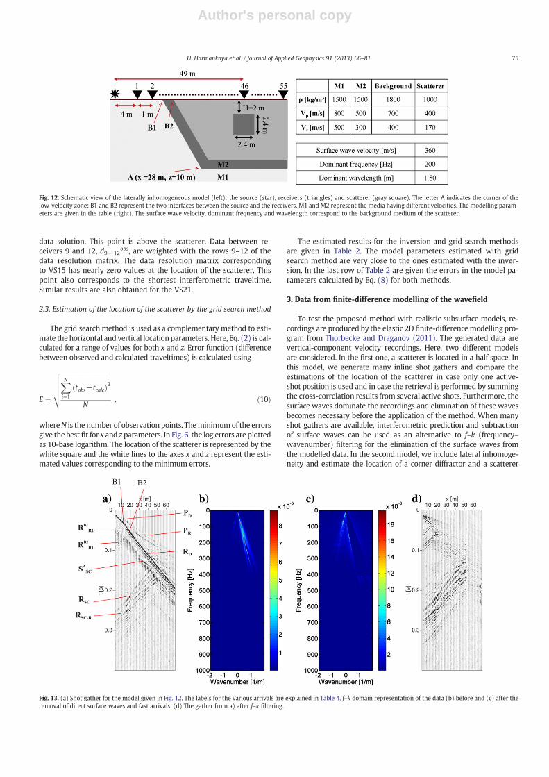
Fig. 12. Schematic view of the laterally inhomogeneous model (left): the source (star), receivers (triangles) and scatterer (gray square). The letter A indicates the corner of thelow-velocity zone; B1 and B2 represent the two interfaces between the source and the receivers. M1 and M2 represent the media having different velocities. The modelling param-eters are given in the table (right). The surface wave velocity, dominant frequency and wavelength correspond to the background medium of the scatterer.

Fig. 13. (a) Shot gather for the model given in Fig. 12. The labels for the various arrivals are explained in Table 4. f–k domain representation of the data (b) before and (c) after theremoval of direct surface waves and fast arrivals. (d) The gather from a) after f–k filtering.



by using scattered body and surface waves, respectively. We show theeffectiveness of the method in the case of lateral variations in themedium.

3.1. Scatterer in a half space

The model consists of a scatterer placed below the surface in a halfspace. The geometry and the medium parameters of the model, whichrepresent a realistic near-surface structure, are given in Fig. 7. A totalof 41 shot gathers are obtained by shifting the source location closerto the scatterer by 0.5 m while keeping the receivers fixed. Fig. 8ashows the shot gather for a shot placed at 1 m from receiver 1. The di-rect P (PD) and Rayleigh (RD) waves, and the scattered Rayleigh (RSC)waves are clearly observed in the figure.

To compare the estimation of the location of the scatterer we usethe result from a single shot with results for summed five shots. Sincethe direct surface waves in these recordings tend to mask the ghostscattered waves in the SI result (Fig. 8b), the estimation of thescattered wavefield is necessary. In the following subsection, thescattered wavefield is obtained by using interferometric predictionand subtraction of surface waves as proposed by Dong et al. (2006).In the rest of the models, we use f–k filtering for the suppression ofthe direct surface wave.

3.1.1. Estimating the location of the scatterer using a single active sourceAdapting the code given in Schuster (2009) for our purpose, the

direct Rayleigh waves from a selected shot gather are eliminated byinterferometric prediction and subtraction (Dong et al., 2006). Thefirst 20 shots are used since the best estimation is obtained by theseshot gathers. Using predictive filtering, the direct surface waves inthe SI result is matched with the direct surface waves in a selected

shot gather. Since the direct surface waves are the dominant compo-nents in either images, the predictive filtering matches the amplitudeand phase of the direct surface waves. Finally, the matched interfero-metric image (Fig. 8c) is subtracted from the selected shot gather(Fig. 8a), leaving a shot gather dominated by the scattered surfacewaves (Fig. 8d).

SI is then applied to the estimated scattered waves (Fig. 8d) usingthe procedure described in Section 2.2. In Fig. 9awe show the estimatedscattered wavefield, while in Fig. 9b–d the retrieved ghost scatteredsurface waves for virtual sources at receivers 1, 21 and 30, respectively(21, 41 and 50 m) are shownwithin the intervals−0.1 and 0.1 s. Com-pared with the SI results of the undisturbed scattered wavefields fromthe previous section (Fig. 3), these ones are somewhat more complexdue the presence of direct surface-wave remnants and other artefacts.

In this model, there are two points that have to be considered:i) the elimination of direct surface waves also eliminates the rightbranch of the scattered field, which has nearly the same slope and fre-quency content as the direct surface wave. Therefore picking thetraveltimes on the right branch is mostly not possible or confident(A in Fig. 9a). ii) When the scatterer is not close to a point scatterer,besides scattering, the wavefield at the scatterer will also undergo re-flection and refraction and will exhibit directionality. Therefore, theright-hand side of the scattered branch will have different slopes. Inthis case, Eq. (2) will not be a good model, since it is valid for apoint scatterer. However, the corner of the scatterer will still generatescattered wavefields and these can be used for location purposes. Inboth cases i and ii, knowing the apex of the scattered wavefield,which can also be approximately determined from a clear shot gather,and the traveltimes at one side of the scattering hyperbola (here,left-side branch, since the source is at the left), we can extrapolatefor the opposite branch by taking the symmetry of the scatteringhyperbola and use it for the estimations of the locations.

Using the ghost-traveltime relation from Eq. (2) and SVD for in-version by Eq. (3), location of the scatterer is estimated using thesame method as described in Section 2.2. The best fit between theobserved and calculated traveltimes of the ghost scattered surfacewaves for virtual sources 1, 21 and 30 (21, 41 and 50 m) are givenin Fig. 10a. The initial (also given in Table 3) and the updated modelparameters after each iteration are given in Fig. 10b. In Fig. 10care shown the estimated model parameters together with their 95%confidence intervals, calculated by Eq. (6), for each of the usedvirtual-source locations. The last value in Fig. 10c is the average

Table 4List of the labelled arrivals in the modelled shot gather given in Fig. 13a.

PD Direct PPR Refracted PRD Direct RayleighRSC Scattered RayleighRSC−R Scattered and Refracted RayleighSSCA Scattered S wave from ARRLB1 Reflected Rayleigh from B1

RRLB2 Reflected Rayleigh from B2

Fig. 14. (a) Extracted scattered surface waves from the panel in Fig. 13d for traveltimes between 0.1 and 0.3 s. Ghost scattered surface waves retrieved by applying seismic inter-ferometry to (a) for virtual-source locations at receivers (b) 26 (29 m), (c) 46 (49 m) and (d) 55 (58 m).



over the results for the different virtual sources; the blue lines repre-sent the actual midpoint, the actual left/right (x) and upper/lower (z)bounds of the scatterer.

For all virtual source positions, it is observed that the errors(Eq. (9)) of the estimated model parameters (x and z) are less than10%, which is similar to the previous example (Table 3). The averageof estimated values are calculated as x=41.31 and z=3.21 meaningerrors 0.76%, 0.4% respectively.

3.1.2. Estimating the location of the scatterer using summation over sev-eral active source

In Fig. 11a we repeat the retrieved ghost scattered surface wavesfrom Fig. 9b for a virtual source at receiver 1. Fig. 11b shows the resultafter summing the retrieved scattered surface waves obtained fromshot gathers from active sources at locations 1 m, 11 m, 21 m, 31 mand 41 m. The direct P- and Rayleighwaves are removed by f–k filteringbefore cross-correlation. The retrieved results in Fig. 11a and b aresimilar, except for some high-frequency oscillations present in thesingle-shot result. These oscillations are especially notable around thetime interval−0.10 s to−0.05 s,when compared to the summed SI re-sult in Fig. 11b. For comparison, the traces of the single-shot (Fig. 11a)and the summed-shot results (Fig. 11b) for receivers 1 (21 m) and 20(40 m) are given in Fig. 11c and d, respectively. We see that the differ-ence between the summed (red line) and single-shot (blue-line) tracesis the elimination of the high-frequency oscillations at the sides ofthe main signal. In the table given in Fig. 11e it can be seen that theestimated results are very close for both cases, since the summationdoes not affect significantly the traveltimes of retrieved ghost scattered

wavefield. In this sense, the method we propose is efficient, since a sin-gle shot is sufficient for estimating the location of the scatterer.

3.2. Laterally inhomogeneous model

To test the proposed method on a more complex model, we runthe finite-difference modelling code for the geometry and mediumparameters as given in Fig. 12. Fig. 13a shows the obtained shot gath-er and the abbreviations used in the figure are given in Table 4. In thismodel, we try to estimate the location of the scatterer from scatteredsurface waves and the location of the corner diffractor (indicated by Ain Fig. 12) from body waves, namely diffracted S-wave, which is indi-cated by Ssc

A in Fig. 13a.Similar to the previous section, removal of the direct Rayleigh

waves is necessary before starting the retrieval of the ghost waves.However, since there is only one shot gather available, the interfero-metric prediction of surface waves is not possible. Instead, an f–k filteris used to remove most of the direct Rayleigh waves and fastest ar-rivals (direct and refracted P-waves). Fig. 13b shows the f–k domainrepresentation of the shot gather in Fig. 13a. After filtering the directsurface waves and the fastest arrivals (Fig. 13c) and transformingback to the t–x (time–distance) domain (Fig. 13d), the scatteredwave field is obtained. To be able to follow the arrival times clearly,a zoomed view of the scattered wavefield is shown in Fig. 14a.

In Fig. 14b–d the retrieved ghost scattered surface waves forvirtual-source locations at receivers 26, (left of the scatterer, 29 m),46 (at the top of the scatterer, 49 m) and 55 (to the right of the scat-terer, 58 m) are given, respectively. To have a closer look at theobtained ghost scattered surface waves, the correlation results are

Fig. 15. (a) Observed (dots) and calculated (solid line) traveltimes; (b) estimated horizontal and vertical locations of the scatterer for the virtual sources 26 (blue, 29 m), 46 (brown,49 m) and 55 (red, 58 m). The values at the zeroth iteration correspond to the initial parameters for the inversion. (c) Estimated model parameters and their 95% confidence limits,blue lines show the actual midpoint and the left/right (x) and upper/lower (z) bounds of the scatterer. (For interpretation of the references to color in this figure legend, the readeris referred to the web version of this article.)

Table 5The actual location (AL), the initial location (IL) for inversion and the estimated model parameters for different virtual source (VS) locations for the scatter given in Fig. 12. Et and Emare the % errors of the traveltimes and model parameters calculated by Eqs. (8) and (9), respectively. σx and σz are standard deviations calculated from the diagonal of the modelcovariance matrix (Eq. (6)) and used in calculation of the 95% confidence levels (1.96 σ).


x 49.00 30.00 48.99 0.02 49.00 0.0 49.54 1.10 49.17 0.35z 3.20 1.00 2.67 16.5 3.35 4.68 3.22 0.62 3.08 3.75∓σX 0.054 0.099 0.210 0.1381∓σZ 0.193 0.130 0.886 0.5294Et (%) 0.0293 0.0512 1.2428



plotted between −0.2 and 0.2 s. Due to the f–k filtering, the rightbranch of the scatterer is filtered-out. We pick the traveltimes fromthe left branch of the scattered wavefield until the apex of the scatter-ing hyperbola. For the right-hand side, we consider the scatterer as apoint scatterer and use the traveltimes of the left part. The obtainedtraveltimes are used in the inversion for the location of the scatterer.The selected ghost traveltime curves are shown in red in Fig. 14b–d.

The location of the scatterer is estimated again by the methodfrom Section 2.2, using the ghost traveltime relation Eq. (2) andSVD for inversion by Eq. (3). The best fit between the observed andcalculated traveltimes of the ghost scattered surface waves for virtualsources 26, 46 and 55 (29, 49 and 58 m) are given in Fig. 15a and theinitial (also given in Table 5) and the updated model parameters foreach iteration are given in Fig. 15b. In Fig. 15c the estimated modelparameters and their 95% confidence limits, obtained by Eq. (6) areshown, for each of the used virtual-source location. The last value is

the average of the individual results. The blue lines in Fig. 15c repre-sent the actual midpoint, the actual left/right (x) and upper/lower (z)bounds of the scatterer. In this example, both the horizontal and ver-tical locations of the scatter are well estimated and they are inside theboundaries of the scatterer. The estimated model parameters, togeth-er with their standard deviation, calculated by Eq. (6), and % error(Eq. (9)), are given in Table 5. Taking the average from the estimatedvalues, we obtain x=49.17 m and z=3.08 m, whose errors are 0.35%and 3.75%, respectively.

To find the location of the corner diffractor, the scattered S-wave isused (Fig. 16a red box). The arrivals other than the scattered S wavesare filtered and muted out. Fig. 16b shows the f–k filtered and mutedshot gather obtained from the shot gather given in Fig. 16a. Theremaining scattered S-wavefield (Fig. 16b) is used in the SI proceduredescribed in Section 2.2. In Fig. 16c–e the retrieved ghost scatteredS-waves for virtual-source locations at receivers 26, (29 m), 30

Fig. 16. (a) Shot gather for the model given in Fig. 12. (b) Extracted scattered S-wave from the shot gather in (a) (red box). Ghost scattered S-wave retrieved by applying seismicinterferometry to (b) for virtual-source locations at receivers (c) 26 (29 m), (d) 30 (33 m) and (e) 34 (37 m). (For interpretation of the references to color in this figure legend, thereader is referred to the web version of this article.)

Fig. 17. (a) Observed (dots) and calculated (solid line) traveltimes; (b) estimated horizontal and vertical location of the corner diffractor for virtual sources 26 (blue, 29 m), 30(brown, 33 m) and 34 (red, 37 m). The values at the zeroth iteration correspond to the initial parameters of the inversion. (c) Estimated model parameters and their 95% confidencelimits, the blue line shows the location of the diffractor labeled A in Fig. 12. (For interpretation of the references to color in this figure legend, the reader is referred to the web ver-sion of this article.)



(33 m) and 34 (37 m) are given, respectively. To have a closer look atthe retrieved scattered S-waves, the correlation results are plottedbetween −0.05 and 0.05 s. The selected ghost traveltime curves areshown in red in Fig. 16c–e.

The location of the corner diffractor is estimated again using theghost traveltime relation Eq. (2) and SVD for inversion by Eq. (3). Thebest fit between the observed and calculated traveltimes of the ghostscattered S-waves for virtual sources 26, 30 and 34 (29, 33 and 37 m)are given in Fig. 17a and the initial (also given in Table 6) and theupdated model parameters for each iteration are given in Fig. 17b.Fig. 17c shows the estimated model parameters and their 95% confi-dence intervals for each of the virtual-source location, while the lastvalue is the average for the different virtual sources. The blue lines inFig. 17c represent the location of the corner diffractor. It can be seenthat the horizontal location is very well estimated. The 95% confidenceinterval includes the actual location of the scatterer. The average fromthe estimated values is x=28.03 m whose error is 0.10%. The estima-tion of the depth for virtual-source location 26 is less accurate whencompared to the virtual-source locations 30 and 34. Note that at the po-sition of this virtual source the recorded scattered S-wave is muchweaker compared to the arrivals at the other traces, which would leadto a relatively poorer correlation result. If we consider the estimationof the depth for virtual-source location 26 as an outlier, than the errorin the estimated averaged depth will be about 0.4% instead of 10%.

4. Discussions

The results from the numerical models show the accuracies we canobtain in practice. The accuracies depend on how well we can isolatethe scattered waves that we want to use for ghost retrieval. In thecase of surface waves, if the direct waves can be adaptively subtracted,we obtain better estimation. But the interferometric adaptive surface-wave subtraction is an expensive operation. The cheaper f–k filteringis a less accurate operation and the result is larger individual errors inthe estimated scatterer location.

In the numerical examples, the velocity is assumed to be a knownparameter and we invert for the location of the scatterer and the cornerdiffractor. On the other hand, the body- and surface-wave velocities canalso be considered as unknown and included in the inversion process;the initial velocities for the inversion can be estimated from the directarrivals of the surface and bodywaves. Since the inverse problem is sen-sitive to the initial parameters, an additional unknown parameter mayaffect the stability of the inversion. Including the velocity as unknownparameter is planned for a future study.

In subsection 3.1.1, we suppressed the direct surface waves by in-terferometric prediction and subtraction. Note that the predictionprocess resulted not only in direct waves, but also in weak scatteredsurface waves (Fig. 8c). If a virtual source is created at a trace wherethe scattered surface-wave arrival has been strongly suppressed, theretrieved ghost scattered surface waves in this virtual-source gatherwould be of a poor quality. As a consequence, application of the inver-sion step to this gather might result in a poor estimation of the scat-terer parameters. Such results should be treated as outliers.

In this study, we considered 2D models. For these situations, onecould attempt estimating location of the scatterers using retrieved

physical surface waves. For the 2D examples, retrieving physicalscattered surface waves is possible as the active sources are alongthe stationary-phase line that connects the receivers and the scat-terers. Note that for 3D problems, locating an offline scatterer maybecome quite difficult when attempting to use retrieved physical ar-rivals from it. To retrieve physical scattered waves in 3D, multiplesources would be required at least in a patch (e.g. Halliday et al.,2010), but in the general case a closed boundary of active sourceswould be required. To understand the effects of a 3D medium in esti-mating the location of the scatterer using our method, both 3Dnumerical modelling and an ultrasonic laboratory experiment areplanned. We expect that, using our method as few as three activesources perpendicular to the line of the receivers would suffice.

In the examples in the previous section, we estimated approxi-mately the midpoint of the scatterer, for which we observed thehighest amplitude of the correlated traces. If the size of the scattereris sufficiently large to allow observation of the scattering from its cor-ner, then the estimation of the size of the scatterer would be possible.Otherwise, the estimations will be within the uncertainty limits.

In themodels in this paper, we considered single isolated scatterers.In case of multiple scatterers, the estimation of the locations could bepossible, if the scattered wavefields of each scatterer can be observedseparately or separated from each other (for example using muting).This can be related to the physical properties, sizes and the distancesbetween the scatterers. If the scatterers are close to one another in awavelength sense, their scattered wavefields will constructively or de-structively interfere and the recorded resulting scattered wavefieldwill be a combination of the two. In such cases, wewould be able to es-timate the parameters of the “combined” scatterer.

Although the examples were for the geotechnical scale, the pro-posed method is not restricted to geotechnical studies only. It canalso be used in exploration and global seismology for detecting andcharacterizing scatterers. For example for the larger scale, locating aburied fault could be possible with our technique.

5. Conclusions

We proposed a method for estimating the location of a near-surfacescatterer or diffractor by using traveltimes of non-physical (ghost)scattered surface and bodywaves obtained by from seismic interferom-etry. The ghost scattered waves are obtained by cross-correlating therecorded scattered waves originating from only one source at the sur-face. The traveltimes of the ghost scattered waves are used in an inver-sion to find the location of the scatterer and a corner diffractor. Thedepth and the horizontal position of the objects are obtained for differ-ent virtual-source locations.

An advantage of our proposed method is that the unwanted travelpaths between the source and the receiver array are eliminated.These travel paths can traverse a complicated medium. Due to theelimination of these paths, the calculation times for waveform inver-sion can be reasonably reduced. Also when lateral changes of the me-dium properties are present, these path effects are eliminated byinterferometry and locations closer to the target are considered forestimation of the location of the scatterer.

Table 6The actual location (AL), the initial location (IL) for inversion and the estimated model parameters for different virtual source (VS) locations for the corner diffractor given in Fig. 12.Et and Em are the % errors of the traveltimes and model parameters calculated by Eqs. (8) and (9), respectively. σx and σz are standard deviations calculated from the diagonal of themodel covariance matrix (Eq. (6)) and used in calculation of the 95% confidence levels (1.96 σ).


x 28.00 35.00 28.13 0.46 28.06 0.21 27.91 0.32 28.03 0.10z 10.00 1.00 6.86 31.4 10.44 4.40 9.63 3.70 8.97 10.23∓σX 0.1680 0.0680 0.0964 0.1185∓σZ 0.2760 0.1030 0.1617 0.1944Et (%) 0.4404 0.1754 0.2830



We tested our method on four numerically modelled datasetswith increasing complexity. We demonstrated that the location ofthe scatterer can be estimated from ghost scattered waves with agood accuracy. We also showed that the quality of the estimated loca-tions of the objects depend on the quality of the estimated scatteredwavefields.

Acknowledgments

This work is supported by TUBITAK (The Scientific and Technologi-cal Research Council of Turkey) with the project 110Y250 titled“DetectingNear-surface Scatterers by Inverse Scattering and Seismic In-terferometry of Scattered Surface Waves” and by Istanbul TechnicalUniversity Research Fund with the project “Estimating the Location ofthe Scatterers by Seismic Interferometry”. We gratefully acknowledgethese financial supports. The investigations of D.D. were supported bythe Division for Earth and Life Sciences (ALW) with financial aid fromthe Netherlands Organization for Scientific Research (NWO). We alsothank the Colorado School of Mines for providing the Seismic Un*x(Cohen and Stockwell, 2012) package as open source software.

References

Al-fares, W., Bakalowicz, M., Guérin, R., Dukhan, M., 2002. Analysis of the karst aquiferstructure of the Lamalou area (Hérault, France) with ground penetrating radar.Journal of Applied Geophysics 51, 97–106.

Bodet, L., Galibert, P.Y., Dhemaied, A., Camerlynck, C., Al-Zoubi, A., 2010. Surface-waveProfiling for Sinkhole Hazard Assessment Along the Eastern Dead Sea Shoreline,Ghor Al-Haditha, Jordan. Extended Abstracts of the 72st EAGE Meeting, Barcelona,p. M027.

Boiero, B., Socco, L.V., 2010. Retrieving lateral variations from surface wave dispersioncurves. Geophysical Prospecting 1–20.

Bozdag, E., Kocaoglu, A.H., 2005. Estimation of site amplifications from shear-wavevelocity profiles in Yesilyurt and Avcilar, Istanbul, by frequency-wavenumber anal-ysis of microtremors. Journal of Seismology 9 (1), 87–98.

Campman, X., Riyanti, C.D., 2007. Non-linear inversion of scattered seismic surfacewaves. Geophysical Journal International 171, 1118–1125.

Campman, X., van Wijk, K., Riyanti, C.D., Scales, J., Herman, G., 2004. Imaging scatteredseismic surface waves. Near Surface Geophysics 2 (4), 223–230.

Canıtez, N., Toksöz, M.N., 1971. Focal mechanism and source depth of earthquakesfrom body- and surface-wave data. Bulletin of the Seismological Society of America61, 1369–1379.

Cardarelli, E., Cercato, M., Cerreto, A., Di Filippo, G., 2010. Electrical resistivity and seis-mic refraction tomography to detect buried cavities. Geophysical Prospecting 58(4), 685–695.

Chai, H.Y., Phoon, K.K., Goh, S.H., Wei, C.F., 2012. Some theoretical and numerical obser-vations on scattering of Rayleigh waves in media containing shallow rectangularcavities. Journal of Applied Geophysics 83, 107–119.

Chang, S., Baag, C., 2005. Crustal structure in Southern Korea from joint analysis ofteleseismic receiver functions and surface-wave dispersion. Bulletin of the Seismo-logical Society of America 95, 1516-1234.

Cohen, J.K., Stockwell Jr., J.W., 2012. CWP/SU: Seismic Un*x Release No. 43: An OpenSource Software Package for Seismic Research and Processing. Center for WavePhenomena, Colorado School of Mines.

Cong, L., Mitchell, B.J., 1998. Seismic velocity and Q structure of the Middle Easterncrust and upper mantle from surface-wave dispersion and attenuation. Pure andApplied Geophysics 153, 503–538.

Culshaw, M.G., Waltham, A.C., 1987. Natural and artificial cavities as ground engineeringhazards. The Quarterly Journal of Engineering Geology 20, 139–150.

Debeglia, N., Bitri, A., Thierry, P., 2006. Karst investigations using microgravity andMASW: application to Orleans, France. Near Surface Geophysics 4, 215–225.

Dong, S., He, R., Schuster, G.T., 2006. Interferometric Prediction and Least-squaresSubtraction of Surface Waves. 76th Annual International Meeting, SEG, ExpandedAbstracts, pp. 2783–2786.

Draganov, D., Wapenaar, K., Mulder, W., Singer, J., Verdel, A., 2007. Retrieval of reflec-tions from seismic background-noise measurements. Geophysical Research Letters34, L04305.

Draganov, D., Campman, X., Thorbecke, J., Verdel, A., Wapenaar, K., 2009. Reflectionimages from ambient seismic noise. Geophysics 74 (5), A63–A67.

Draganov, D., Heller, K., Ghose, R., 2012. Monitoring CO2 storage using ghost reflectionsretrieved from seismic interferometry. International Journal of Greenhouse GasControl 11S, S35–S46.

Edmonds, C.N., 2008. Karst and mining geohazards with particular reference to theChalk outcrop, England. Quarterly Journal of Engineering Geology & Hydrogeology41, 261–278.

Ekström, G., 2006. Global detection and location of seismic sources by using surfacewaves. Bulletin of the Seismological Society of America 96 (4A), 1201–1212.

Engelsfeld, T., Šumanovac, F., Pavin, N., 2008. Investigation of underground cavities in atwo-layer model using the refraction seismic method. Near Surface Geophysics 6(4), 221–231.

Engelsfeld, T., Šumanovac, F., Krstić, V., 2011. Classification of near-surface anomaliesin the seismic refraction method according to the shape of the time–distancegraph: a theoretical approach. Journal of Applied Geophysics 74 (1), 59–68.

Foti, S., 2000. Multistation Methods for Geotechnical Characterization using RayleighWaves. Ph.D. dissertation, Ingegneria Geotecnica, Universuty deli Studi.

Gelis, C., Leparoux, D., Virieux, J., Bitri, A., Operto, S., Grandjean, G., 2005. Numericalmodeling of surface waves over shallow cavities. Journal of Environmental andEngineering Geophysics 10 (2), 111–121.

Grandjean, G., Leparoux, D., 2004. The potential of seismic methods for detecting cavitiesand buried objects: experimentation at a test site. Journal of Applied Geophysics 56(2), 93–106.

Halliday, D.F., Curtis, A., 2008. Seismic surface waves in a suburban environment: activeand passive interferometric methods. The Leading Edge 27 (2), 210–218.

Halliday, D.F., Curtis, A., 2009. Seismic interferometry of scattered surface waves inattenuative media. Geophysical Journal International 185, 419–446.

Halliday, D.F., Curtis, A., Robertsson, J.O.A., van Manen, D.J., 2007. Interferometricsurface-wave isolation and removal. Geophysics 72 (5), A69–A73.

Halliday, D.F., Curtis, A., Vermeer, P., Strobbia, C., Glushchenko, A., van Manen, D.J.,Robertsson, J.O.A., 2010. Interferometric ground-roll removal: attenuation ofscattered surface waves in single-sensor data. Geophysics 75 (2), A15–A25.

Harmankaya, U., Kaslilar, A., Thorbecke, J., Wapenaar, K., Draganov, D., 2012a. Estimat-ing the Location of Scatterers by Seismic Interferometry of Scattered SurfaceWaves. Extended Abstracts of the 74st EAGE Meeting, Copenhagen, p. X008.

Harmankaya, U., Kaslilar, A., Thorbecke, J., Wapenaar, K., Draganov, D., 2012b. Estimationof the Location of a Scatterer from Interferometric Ghosts of the Scattered SurfaceWaves. Extended Abstracts of the Istanbul International Geophysical Conferenceand Oil & Gas Exhibition, Istanbul, p. 173.

Herman, G.C., Milligan, P.A., Huggins, R.J., Rector, J.W., 2000. Imaging shallow objectsand heterogeneities with scattered guided waves. Geophysics 65 (1), 247–252.

Kaslilar, A., 2007. Inverse scattering of surface waves: imaging of near-surface hetero-geneities. Geophysical Journal International 171, 352–367.

Khomenko, V.P., 2008. Forecast of a collapse location: new approach. Quarterly Journalof Engineering Geology & Hydrogeology 41, 393–401.

Kimman, W.P., Trampert, J., 2010. Approximations in seismic interferometry and theireffects on surface waves. Geophysical Journal International 182, 461–476.

King, S., Curtis, A., 2012. Suppressing nonphysical reflections in Green's function esti-mates using source-receiver interferometry. Geophysics 77, Q15–Q25.

Kocaoglu, A.H., Fırtana, K., 2011. Estimation of shear wave velocity profiles by the in-version of spatial autocorrelation coefficients. Journal of Seismology 15 (4),613–624.

Kovach, R.L., 1978. Seismic surface waves and crustal and upper mantle structure.Review of Geophysics and Space Physics 16, 1–13.

Leparoux, D., Bitri, A., Grandjean, G., 2000. Underground cavity detection: a new methodbased on seismic Rayleigh waves. EJEEG 5, 33–53.

McCann, D.M., Jackson, P.D., Culshaw, M.G., 1987. The use of geophysical surveyingmethods in the detection of natural cavities and mineshafts. The Quarterly Journalof Engineering Geology 20, 59–73.

Mikesell, T.D., vanWijk, K., Blum, T.E., 2012. Analyzing the coda from correlating scatteredsurface waves. Journal of the Acoustic Society of America 131 (3), EL275–EL281.

Mohanty, P.R., 2011. Numerical modeling of P-waves for shallow subsurface cavitiesassociated with old abandoned coal workings. Journal of Environmental and Engi-neering Geophysics 16 (4), 165–175.

Nasseri-Moghaddam, A., Cascante, G., Jean Hutchinson, J., 2005. A new quantitativeprocedure to determine the location and embedment depth of a void using surfacewaves. Journal of Environmental and Engineering Geophysics 10 (1), 51–64.

Nazarian, S., Stokoe, K.H., Hudson, W.R., 1983. Use of spectral analysis of surface wavesmethod for determination of moduli and thicknesses of pavement systems. Trans-portation Research Record 930, 38–45.

Nuzzo, L., Leucci, G., Negri, S., 2007. GPR, VES and refraction seismic surveys in thekarstic area “Spedicaturo” near Nociglia (Lecce, Italy). Near Surface Geophysics 5(1), 67–76.

O'Neill, A., 2003. Full waveform reflectivity for modeling, inversion and appraisal ofseismic surface wave dispersion in shallow site investigations. Ph.D. dissertation,University of Western Australia, Perth.

Park, C.B., Miller, R.D., Xia, J., 1999. Multichannel analysis of surface waves. Geophysics64 (3), 800–808.

Randall, M.R., Zandt, G., 2007. Inverse Problems in Geophysics, Lecture Notes, Dept. ofGeosciences, University of Arizona, Tucson, Arizona 8521.

Rix, G.J., Hebeler, G.L., Orozco, M.C., 1998. Near-surface Vs profiling in the New Madridseismic zone using surface wave methods. Seismological Research Letters 73 (3),380–392.

Rodríguez-Castellanos, A., Sánchez-Sesma, F.J., Luzón, F., Martin, R., 2006. Multiplescattering of elastic waves by subsurface fractures and cavities. Bulletin of the Seis-mological Society of America 96 (4A), 1359–1374.

Roux, P., Sabra, K.G., Gerstoft, P., Kuperman, W.A., Fehler, M.C., 2005. P-waves from cross-correlation of seismic noise. Geophysical Research Letters 32, L193031–L193034.

Ruigrok, E., Campman, X., Draganov, D., Wapenaar, K., 2010. High-resolution litho-spheric imaging with seismic interferometry. Geophysical Journal International183, 339–357.

Samyn, K., Bitri, A., Grandjean, G., 2012. Imaging a near-surface feature using cross-correlation analysis of multi-channel surface wave data. Near Surface Geophysics10. http://dx.doi.org/10.3997/1873-0604.2012007.

Schuster, G.T., 2009. Seismic Interferometry. Cambridge University Press, Cambridge.



Schuster, G.T., Yu, J., Sheng, J., Rickett, J., 2004. Interferometric/daylight seismic imaging.Geophysical Journal Internatinal 157, 838–852.

Sens-Schönfelder, C., Wegler, U., 2006. Passive image interferometry and seasonal var-iations of seismic velocities at Merapi volcano, Indonesia. Geophysical ResearchLetters 33, L21302.

Shapiro, N.M., Campillo, M., 2004. Emergence of broadband Rayleigh waves from cor-relations of the ambient seismic noise. Geophysical Research Letters 31, L07614.

Snieder, R., 1987. Surface wave holography. In: Nolet, G. (Ed.), Seismic tomography. D.Reidel Publishing, Dordrecht, pp. 323–337.

Snieder, R., 2004. Extracting the Green's function from the correlation of coda waves: aderivation based on stationary phase. Physical Review E 69, 046610.

Snieder, R., Wapenaar, K., 2010. Imaging with ambient noise. Physics Today 63 (9),44–49.

Snieder, R., Wapenaar, K., Larner, K., 2006. Spurious multiples in seismic interferometryof primaries. Geophysics 71, SI111–SI124.

Socco, L.V., Boiero, D., 2008. Improved Monte Carlo inversion of surface wave data.Geophysical Prospecting 56, 357–371.

Socco, L.V., Boiero, D., Wisén, R., Foti, S., 2009. Laterally constrained inversion of groundroll of seismic reflection records. Geophysics 74 (6), G35–G45.

Socco, L.V., Jongmans, D., Boiero, D., Stocco, S., Tokeshi, K., Maraschini, M., Hantz, D.,2010. Geophysical investigation of the Sandalp rock avalanche deposits. Journalof Applied Geophysics 70 (4), 277–291.

Thorbecke, J., Draganov, D., 2011. Finite-difference modeling experiments for seismic in-terferometry. Geophysics 75, H1–H18. http://dx.doi.org/10.1190/GEO2010-0039.1.

van Manen, D., Curtis, A., Robertsson, J.O.A., 2006. Interferometric modeling of wavepropagation in inhomogeneous elastic media using time reversal and reciprocity.Geophysics 71 (4), SI47–SI60.

Wapenaar, K., 2004. Retrieving the elastodynamic Green's function of an arbitrary in-homogeneous medium by cross correlation. Physical Review Letters 93 (25),254301.

Wapenaar, K., Fokkema, J., 2006. Green's function representations for seismic interfer-ometry. Geophysics 71 (4), SI33–SI46.

Woodcock, N.H., Omma, J.E., Dickson, J.A.D., 2006. Chaotic breccia along the Dent Fault,NW England: implosion or collapse of a fault void? Journal of the Geological Soci-ety 163, 431–446.

Xia, J., Nyquist, J.E., Xu, Y.X., Roth, M.J.S., Miller, R.D., 2007. Feasibility of detecting near-surface feature with Rayleigh-wave diffraction. Journal of Applied Geophysics 62(3), 244–253.

Xia, J., Xu, Y., Miller, R.D., Zeng, C., 2010. A trade-off solution between model resolutionand covariance in surface-wave inversion. Pure and Applied Geophysics 167 (12),1537–1547.

Xu, C., Butt, S.D., 2006. Evaluation of MASW techniques to image steeply dipping cavi-ties in laterally inhomogeneous terrain. Journal of Applied Geophysics 59 (2),106–116.


Author's personal copy -...

Documents

Transcript of Author's personal copy -...