National River Health Program healthy rivers living rivers

rivers for life MONITORING RIVER HEALTH INITIATIVE TECHNICAL REPORT REPORT NUMBER 21

Australian River Assessment System: Review of Physical River Assessment Methods — A Biological Perspective Authors: Melissa Parsons Martin Thoms Richard Norris

Published By: Environment Australia GPO Box 787 CANBERRA ACT 2601

Authors: Melissa Parsons, Martin Thoms and Richard Norris

Cooperative Research Centre for Freshwater Ecology University of Canberra ACT 2601 Telephone: 02 6201 5408 Fax: 02 6201 5038

Copyright: University of Canberra and Commonwealth of Australia This work is copyright. Information contained in this publication may be copied or

reproduced for study, research, information, or educational purposes, subject to inclusion of an acknowledgment of the source. Requests and inquiries concerning reproduction and rights should be addressed to the above authors and:

Assistant Secretary

Water Branch Environment Australia GPO Box 787 Canberra ACT 2601

Disclaimer: The views and opinions expressed in this publication are those of the authors and do

not necessarily reflect those of the Commonwealth Government or the Minister for the Environment and Heritage.

While reasonable efforts have been made to ensure that the contents of this

publication are factually correct, the Commonwealth does not accept responsibility for the accuracy or completeness of the contents, and shall not be liable for any loss or damage that may be occasioned directly or indirectly through the use of, or reliance on, the contents of this publication.

The information contained in this work has been published by Environment Australia

to help develop community, industry and management expertise in sustainable water resources management and raise awareness of river health issues and the needs of our rivers. The Commonwealth recommends that readers exercise their own skill and care with respect to their use of the material published in this report and that users carefully evaluate the accuracy, currency, completeness and relevance of the material for their purposes.

Citation: For bibliographic purposes this report may be cited as:

Parsons, M., Thoms, M. and Norris, R., 2002, Australian River Assessment System: Review of Physical River Assessment Methods — A Biological Perspective, Monitoring River Heath Initiative Technical Report no 21, Commonwealth of Australia and University of Canberra, Canberra.

ISBN: 0 642 54887 0 ISSN: 1447-1280 Information: For additional information about this publication, please contact the author(s).

Alternatively, you can contact the Community Information Unit of Environment Australia on toll free 1800 803 772.

REVIEW OF PHYSICAL RIVER ASSESSMENT

METHODS: A BIOLOGICAL PERSPECTIVE

Melissa Parsons

Martin Thoms

Richard Norris

Cooperative Research Centre for Freshwater Ecology

April 2000

A report to Environment Australia for the AUSRIVAS Physical and

Chemical Assessment Module

i

ACKNOWLEDGMENTS

The aim of this document is to review existing stream assessment methods and as such,

it draws heavily on published material. In describing the details of each method, it was

sometimes difficult to diverge greatly from the existing text. Thus, we would like to

acknowledge the creators of each stream assessment method, because this review is

merely a summary of their expertise. These authors are:

State of the Rivers Survey John Anderson

Index of Stream Condition Lindsay White, Tony Ladson

Habitat Predictive Modelling Nerida Davies, Richard Norris, Martin

Thoms

Geomorphic River Styles Gary Brierley, Kirstie Fryirs, Tim Cohen

HABSCORE James Plafkin, Michael Barbour,

Kimberley Porter, Sharon Gross, Robert

Hughes, Jeroen Gerritson, Blaine Snyder,

James Stribling

River Habitat Survey P. Raven, N. Holmes, F. Dawson, P. Fox,

M. Everard, I. Fozzard, K. Rouen, among

others

AUSRIVAS All people involved with the National

River Health Program

However, it should be noted that the information supplied in this report is a synthesis

and interpretation of published material and any misinterpretations, although

unintentional, are the sole responsibility of the authors.

ii

TABLE OF CONTENTS

1 Introduction............................................................................................................. 2

1.1 The physical and chemical assessment module..........................................................................2

1.2 Review of stream assessment methods........................................................................................2

2 Review of river assessment methods ..................................................................... 2

2.1 Scope and rationale ......................................................................................................................2

2.2 AUSRIVAS....................................................................................................................................22.2.1 How did AUSRIVAS come about? ......................................................................................22.2.2 How does AUSRIVAS work?...............................................................................................22.2.3 How does AUSRIVAS assess stream condition? .................................................................22.2.4 How does AUSRIVAS link physical and chemical features with the biota?........................2

2.3 HABSCORE (USEPA Rapid Bioassessment Protocols) ...........................................................22.3.1 How did HABSCORE come about? .....................................................................................22.3.2 How does HABSCORE work? .............................................................................................22.3.3 How does HABSCORE assess stream condition? ................................................................22.3.4 How does HABSCORE link physical and chemical features with the biota?.......................2

2.4 Index of Stream Condition ..........................................................................................................22.4.1 How did the Index of Stream Condition come about? ..........................................................22.4.2 How does the Index of Stream Condition work? ..................................................................22.4.3 How does the Index of Stream Condition assess stream condition? .....................................22.4.4 How does the Index of Stream Condition link physical and chemical features with

the biota?...............................................................................................................................2

2.5 Geomorphic River Styles .............................................................................................................22.5.1 How did Geomorphic River Styles come about? ..................................................................22.5.2 How does Geomorphic River Styles work? ..........................................................................22.5.3 How does Geomorphic River Styles assess stream condition? .............................................22.5.4 How does Geomorphic River Styles link physical and chemical features with

the biota?...............................................................................................................................2

2.6 State of the Rivers Survey............................................................................................................22.6.1 How did the State of the Rivers Survey come about?...........................................................22.6.2 How does the State of the Rivers Survey work?...................................................................22.6.3 How does the State of the Rivers Survey assess stream condition?......................................22.6.4 How does the State of the Rivers Survey link physical and chemical features with

the biota?...............................................................................................................................2

2.7 Habitat Predictive Modelling ......................................................................................................22.7.1 How did Habitat Predictive Modelling come about? ............................................................22.7.2 How does Habitat Predictive Modelling work? ....................................................................22.7.3 How does Habitat Predictive Modelling assess stream condition? .......................................22.7.4 How does Habitat Predictive Modelling link physical and chemical features with the biota?

2

2.8 River Habitat Survey ...................................................................................................................22.8.1 How did the River Habitat Survey come about?...................................................................22.8.2 How does the River Habitat Survey work?...........................................................................22.8.3 How does the River Habitat Survey assess stream condition?..............................................22.8.4 How does the River Habitat Survey link physical and chemical features with

the biota?...............................................................................................................................2

iii

3 Summary and evaluation of river assessment methods ...................................... 2

3.1 Summary of river assessment methods.......................................................................................23.1.1 AUSRIVAS ..........................................................................................................................23.1.2 HABSCORE .........................................................................................................................23.1.3 Index of Stream Condition....................................................................................................23.1.4 Geomorphic River Styles ......................................................................................................23.1.5 State of the Rivers Survey.....................................................................................................23.1.6 Habitat Predictive Modelling ................................................................................................23.1.7 River Habitat Survey.............................................................................................................2

3.2 Evaluation of river assessment methods.....................................................................................2

3.3 Future directions - habitat assessment workshop......................................................................2

4 References................................................................................................................ 2

1

1 INTRODUCTION

1.1 The physical and chemical assessment module

The Australian River Assessment System (AUSRIVAS) is a nationally standardised

approach to biological assessment of stream condition using macroinvertebrates (Coysh

et al., 2000). It was developed under the auspices of the National River Health Program

(NRHP). Within the AUSRIVAS component of the NRHP, a suite of 'toolbox' projects

have been commissioned with the aim of either refining the existing assessment

techniques, or developing additional aspects of river health assessment that are

complementary to those made by the AUSRIVAS macroinvertebrate predictive models

(O'Connor, 1999). One of these projects is the development of a physical and chemical

assessment module.

One of the main aims of the physical and chemical assessment module is to develop a

standardised protocol for the physical and chemical assessment of stream condition, that

will complement the biological assessments of stream condition made using

AUSRIVAS. Disregarding the chemical component for now, development of such a

protocol requires simultaneous consideration of stream condition from a biological and

a physical perspective. While there would seem to be obvious interdependencies

between the physical and biological components of streams, merging the two

components is, in reality, a complex task because of the different paradigms that exist

within the disciplines of stream ecology and fluvial geomorphology. The physical and

chemical assessment module represents a first step in bringing together biological and

physical or geomorphological approaches to the assessment of stream condition.

However, in developing a standardised protocol for physical assessment of stream

condition, that is directly relevant to biological assessment of stream condition, several

questions become apparent:

• which physical variables are related to the distribution and abundance of biota?;

• how might geomorphological process variables, that describe the formation of

habitats, be related to biota?;

• are there any geomorphological process variables that are unrelated to biota but

which are useful for describing the condition of a stream from a physical

perspective?;

2

• at which scales are biota related to different habitat components?; and,

• can geomorphological process variables be measured within the 'rapid'

biomonitoring philosophy, while still retaining the necessary levels of precision

and accuracy?

1.2 Review of stream assessment methods

The common link between assessment of stream condition from a biological and a

geomorphological perspective is the expression of stream habitat, or physical structure,

as a templet for biological communities. From a biological perspective, the physical

habitat is considered as a templet upon which the ecological organisation and dynamics

of ecosystems are observed (Townsend and Hildrew, 1994; Montgomery, 1999; Norris

and Thoms, 1999). Thus, measurement of biological habitat tends to include the factors

that directly influence biotic communities, at scales relevant to the organism of interest

(Weins, 1989; Cooper et al., 1998; Sale, 1998) or the disturbance of interest (Rankin,

1995). From a geomorphological perspective, the expression of physical habitat is

related to a set of predictable geomorphic processes (Harper and Everard, 1998; Muhar

and Jungwirth, 1998; Brierley et al., 1999; Montgomery, 1999). The pattern of stream

habitat that forms as a result of these processes provides the templet for biotic

communities. Thus, measurement of geomorphological habitat tends to consider fluvial

processes as they relate to channel structure, at scales that reflect the hierarchical

organisation of stream systems (Schumm; 1977; Frissell et al., 1986; Maddock, 1999).

Regardless of how each perspective views habitat, the common ground between

geomorphology and biology is that both disciplines consider that a 'healthy' habitat is

vital for a 'healthy' biotic community and indeed, for a 'healthy' stream ecosystem

(Maddock, 1999; Norris and Thoms, 1999).

Biological monitoring programs are used worldwide to assess stream condition. The

use of biota to assess stream condition has numerous advantages, the most prominent

being that biotic communities are affected by a multitude of chemical and physical

influences (Rosenberg and Resh, 1993). Thus, condition of the biota is a reflection of

the overall condition of the stream ecosystem (Reice and Wohlenberg, 1993). However,

there are numerous methods that have been developed to assess the physical or

geomorphological condition of streams and which have the potential to enhance the

interpretation of biological assessments of stream condition, or to provide information

3

on stream condition that is not directly apparent within biological assessment. Any

attempt to merge aspects of biological assessment with aspects of physical condition

must identify the physical features that are of importance to the biota (Harper et al.,

1995; Maddock, 1999), while retaining aspects that may be important to the physical

formation of stream habitat.

The aim of this document is to review methods for the assessment of stream condition

that are potential candidates for inclusion in a nationally standardised physical and

chemical assessment protocol. It is not the aim of this document to make final

recommendations for the format of the protocol. Rather, this review forms an initial

information base and will be used in conjunction with a habitat assessment workshop to

make final recommendations for a physical (and chemical) stream assessment protocol.

The focus of this review is on assessment of the physical and geomorphological aspects

of stream condition, with consideration of the potential for each method to link physical

condition with ecological condition. It will answer four questions about each method:

1. How did the method come about?

Describes the scientific context and river management background of the

method.

2. How does the method work?

Provides an overview of the mechanics of the method including the variables

collected in the field or laboratory, the methods used to collect the data, and the

data analysis.

3. How does the method assess stream condition?

Explains the approach of the method to the assessment of stream condition and

considers factors such as predictive ability, definition and use of a reference

condition and the philosophies used to determine deviation from this unimpaired

reference condition.

4. How does the method link physical and chemical features with the biota?

Examines how the method implicitly or explicitly links the physical assessment

of stream condition with biota, or in some cases, biotic condition.

The final section of the review will summarise the advantages and disadvantages of

each physical assessment method and evaluate the potential for each method to

encompass the physical aspects of river condition that are relevant to stream biota.

4

2 REVIEW OF RIVER ASSESSMENT METHODS

2.1 Scope and rationale

There are many stream assessment methods that have been developed worldwide. The

methods chosen for inclusion in this review represent the suite of approaches currently

in use in Australia. The State of the Rivers Survey, Index of Stream Condition and

Geomorphic River Styles methods were developed for, and tested in, Australian rivers

and streams. Thus, they tend to have an ability to incorporate stream features inherent

to Australian conditions such as high flow variability, high turbidity and complex

channel morphology. Although based on a method developed in the United Kingdom,

the AUSRIVAS and Habitat Predictive Modelling methods have been successfully

adapted to Australian conditions. In particular, AUSRIVAS is a nationally standardised

and predictive approach to biological assessment that has recently been used to

determine the condition of around 6000 river sites across Australia. The United States

Environmental Protection Agency's HABSCORE method of stream assessment was

used within the AUSRIVAS predictive model and thus, is included in this review. The

River Habitat Survey is not currently being applied in Australia. However, it is

included in this review because it represents an approach that was applied on a national

scale in the United Kingdom, to assess the physical condition of streams and rivers.

There are some additional methods of stream assessment that were not included in the

review. The Integrated Habitat Assessment System (IHAS) has been developed in

South Africa and is used in conjunction with the country's rapid biological assessment

program (McMillan, 1998). The IHAS measures components of the stream habitat

relevant to macroinvertebrates, such as substratum, vegetation and physical stream

condition. These components are rated and a score representing a continuum of habitat

quality is derived. Another method, Pressure-Habitat-Biota (PBH), has been developed

for use in small to medium sized rivers and streams in New South Wales (Chessman

and Nancarrow, 1999). PBH measures variables representing the pressures on streams

(e.g. physical restructuring, water pollution and introduced species), the habitat of

streams (e.g. habitat area, habitat diversity and habitat stability) and the biota within

streams (e.g. diatoms, riparian vegetation, water plants, macroinvertebrates and fish).

These variables are then compared with each other to:

• determine current stream condition;

5

• identify ecological assets;

• identify ecological problems;

• improve understanding of cause and effect relationships between biota and

habitat or pressures; and,

• provide an ecosystem stress classification of stream sub-catchments (Chessman

and Nancarrow, 1999).

In addition to the IHAS and PBH methods, the United Kingdom's System for

Evaluating Rivers for Conservation (SERCON) was also omitted from this review.

SERCON is designed to assess the conservation value of rivers according to criteria of

physical diversity, naturalness, representativeness, rarity, species richness and special

features (Boon et al., 1998). Field data are collected using an extended version of the

River Habitat Survey, and other data are gathered from a range of sources. Rating

scores are derived for each variable and these scores are subsequently combined to

produce indices for each of the conservation criteria described above (Boon et al.,

1998).

Overall, the rationale for omission of IHAS, PBH and SERCON from this review is

somewhat subjective and has no relationship to the mechanisms that each method uses

to assess stream condition. Rather, the IHAS and PBH methods were omitted because

they are still in the development stage and thus, there was a limited amount of literature

available. SERCON is a complex system for evaluating conservation potential and

thus, it was decided that the inclusion of SERCON's smaller sibling, the River Habitat

Survey, would provide an adequate description of the potential for this method to assess

physical stream condition.

6

2.2 AUSRIVAS

2.2.1 How did AUSRIVAS come about?

The Australian River Assessment System (AUSRIVAS) was developed in response to

the need for a nationally standardised method to assess the ecological condition of

Australia's river systems (Simpson and Norris, 2000). The AUSRIVAS approach is

based on the British River InVertebrate Predication and Classification System

(RIVPACS, Wright et al., 1984; Moss et al., 1987), which has been successfully used to

assess the quality of rivers in the U.K. (Wright et al., 1998). Initially, the adoption of

RIVPACS to Australian conditions required modifications to the sampling design and

statistical analysis components (Simpson and Norris, 2000). The major advantage of

the AUSRIVAS and RIVPACS approaches to river assessment is that the fauna

expected to occur at a site can be predicted, forming a 'target' community against which

to measure potential ecological impairment.

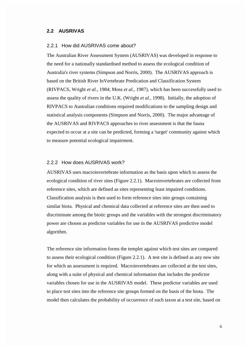
2.2.2 How does AUSRIVAS work?

AUSRIVAS uses macroinvertebrate information as the basis upon which to assess the

ecological condition of river sites (Figure 2.2.1). Macroinvertebrates are collected from

reference sites, which are defined as sites representing least impaired conditions.

Classification analysis is then used to form reference sites into groups containing

similar biota. Physical and chemical data collected at reference sites are then used to

discriminate among the biotic groups and the variables with the strongest discriminatory

power are chosen as predictor variables for use in the AUSRIVAS predictive model

algorithm.

The reference site information forms the templet against which test sites are compared

to assess their ecological condition (Figure 2.2.1). A test site is defined as any new site

for which an assessment is required. Macroinvertebrates are collected at the test sites,

along with a suite of physical and chemical information that includes the predictor

variables chosen for use in the AUSRIVAS model. These predictor variables are used

to place test sites into the reference site groups formed on the basis of the biota. The

model then calculates the probability of occurrence of each taxon at a test site, based on

7

Figure 2.2.1 Schematic representation of AUSRIVAS assessment of site condition.

Macroinvertebrate and phys/cheminformation collected

Groups formed on the basis ofmacroinvertebrates

Phys/chem variables used todiscriminate between

macroinvertebrate groups

Variables with the strongestdiscriminatory power chosen

as predictor variables

Macroinvertebrate and phys/cheminformation collected

Test site information enteredinto AUSRIVAS predictivemodel. Test sites matchedwith reference site groupsusing predictor variables

AUSRIVAS predictive modelalgorithms developed using

predictor variables andmacroinvertebrate information

Probability of taxonoccurrence at a test site is

calculated on the basis of theoccurrence of taxa within

reference site groups

The number of taxa expectedto occur is compared againstthe number of taxa that werecollected at the test site. Thedifference between the two(observed:expected ratio) is

an indicator of biologicalcondition at a test site

TEST SITESREFERENCE SITES

8

the occurrence of each taxon within the corresponding reference site groups. The

number of taxa predicted to occur at a test site is compared against the number of taxa

that were actually collected at the test site, with the difference between the two being an

indication of the ecological condition of the site.

2.2.3 How does AUSRIVAS assess stream condition?

Macroinvertebrates are a commonly used group of organisms in the biological

monitoring of water quality (Rosenberg and Resh, 1993). From an ecological

perspective, the advantages of using macroinvertebrates to assess river condition are

that they are common in many different river habitats, they show responses to a wide

range of environmental stresses and they act as continuous monitors of the water that

they inhabit (Rosenberg and Resh, 1993). Thus, the ecological foundation upon which

biological monitoring is based is that the structure of the benthic macroinvertebrate

community indicates the state of the entire ecosystem (Reice and Wohlenberg, 1993).

AUSRIVAS assesses site condition by comparing the macroinvertebrates that are

predicted to occur at a test site, with the macroinvertebrates that were collected at a test

site. The deviation between the number of taxa expected to occur and the number of

taxa that were actually observed (observed:expected ratio) is a measure of the ecological

condition of a site. If the number, or type, of taxa collected at a test site does not fulfil

expectations, then it is likely that water quality or habitat conditions are limiting the

biological potential of the site. The observed:expected ratio ranges from 0 to > 1 and

represents a continuum of ecological condition. For ease of interpretation, the

continuum can be broken into bands that delineate an ecological condition that is

impoverished, well below reference, below reference, reference, and richer than

reference (Simpson and Norris, 2000).

The robustness of AUSRIVAS assessments of site condition are enhanced through the

use of a regional reference condition approach (Reynoldson et al., 1997). Comparison

of test sites to groups of reference sites that represent an array of potential regional

conditions enables prediction of the taxa likely to occur at sites with given

environmental characteristics (Moss et al., 1987; Reynoldson et al., 1997). In

predicting the taxa that should occur at a test site, the AUSRIVAS model calculates the

weighted probabilities of a test site belonging to each of the reference site groups, which

9

in turn enables natural variation in macroinvertebrate habitat associations to be

accounted for before determining site condition. However, there are several limitations

of the AUSRIVAS predictive models that currently have the potential to affect

assessments of site condition. First, to allow accurate matching of test sites with

reference site groups, reference sites must cover a wide range of river types. Secondly,

evaluation of whether macroinvertebrate community impairment detected by

AUSRIVAS is likely to be caused by water quality degradation, habitat degradation, or

a combination of both is highly dependent upon the collection of the appropriate

supporting data from each test site.

2.2.4 How does AUSRIVAS link physical and chemical features with the biota?

The fundamental assumption behind AUSRIVAS is that the physical and chemical

factors measured at any site are directly related to the macroinvertebrates. This

assumption is derived from a multitude of studies that have demonstrated specific

physical and chemical influences on macroinvertebrate community structure in streams

(Resh and Rosenberg, 1984; Vinson and Hawkins, 1998; Ward, 1992). The empirical

evidence linking macroinvertebrates with their environmental requirements provides a

strong foundation for the process that AUSRIVAS uses to link physical and chemical

variables to taxon occurrence, and the subsequent assessments of ecological condition

that are derived from this information.

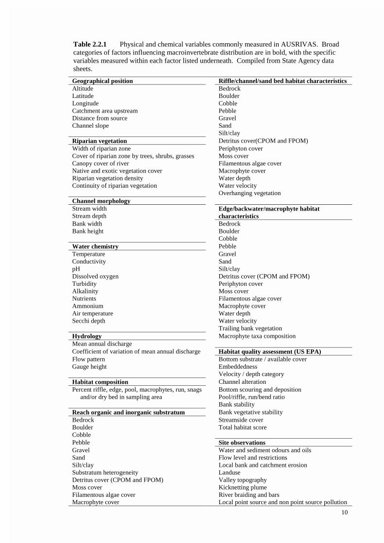
The physical and chemical variables collected in AUSRIVAS broadly encompass the

factors that influence the distribution of macroinvertebrates on a catchment, reach and

individual habitat scale. These factors are geographical position, riparian vegetation,

channel morphology, water chemistry, habitat composition, habitat characteristics,

organic substratum, inorganic substratum and hydrology (Table 2.2.1). Within each

factor, a number of different variables are measured to represent specific influences on

macroinvertebrate communities (Table 2.2.1). In addition, the US EPA habitat

assessment (see Section 2.3) is also performed at each site and a suite of observations

that indicate potential human influences are recorded and used to aid interpretation of

AUSRIVAS biological outputs (Table 2.2.1). However, there are several shortcomings

of the physical and chemical data that may affect the AUSRIVAS assessments of

ecological condition. Firstly, AUSRIVAS sampling is conducted by State agencies. As

10

Table 2.2.1 Physical and chemical variables commonly measured in AUSRIVAS. Broadcategories of factors influencing macroinvertebrate distribution are in bold, with the specificvariables measured within each factor listed underneath. Compiled from State Agency datasheets.

Geographical position Riffle/channel/sand bed habitat characteristicsAltitude BedrockLatitude BoulderLongitude CobbleCatchment area upstream PebbleDistance from source GravelChannel slope Sand

Silt/clayRiparian vegetation Detritus cover(CPOM and FPOM)Width of riparian zone Periphyton coverCover of riparian zone by trees, shrubs, grasses Moss coverCanopy cover of river Filamentous algae coverNative and exotic vegetation cover Macrophyte coverRiparian vegetation density Water depthContinuity of riparian vegetation Water velocity

Overhanging vegetationChannel morphologyStream widthStream depth

Edge/backwater/macrophyte habitatcharacteristics

Bank width BedrockBank height Boulder

CobbleWater chemistry PebbleTemperature GravelConductivity SandpH Silt/clayDissolved oxygen Detritus cover (CPOM and FPOM)Turbidity Periphyton coverAlkalinity Moss coverNutrients Filamentous algae coverAmmonium Macrophyte coverAir temperature Water depthSecchi depth Water velocity

Trailing bank vegetationHydrology Macrophyte taxa compositionMean annual dischargeCoefficient of variation of mean annual discharge Habitat quality assessment (US EPA)Flow pattern Bottom substrate / available coverGauge height Embeddedness

Velocity / depth categoryHabitat composition Channel alterationPercent riffle, edge, pool, macrophytes, run, snags and/or dry bed in sampling area

Bottom scouring and depositionPool/riffle, run/bend ratioBank stability

Reach organic and inorganic substratum Bank vegetative stabilityBedrock Streamside coverBoulder Total habitat scoreCobblePebble Site observationsGravel Water and sediment odours and oilsSand Flow level and restrictionsSilt/clay Local bank and catchment erosionSubstratum heterogeneity LanduseDetritus cover (CPOM and FPOM) Valley topographyMoss cover Kicknetting plumeFilamentous algae cover River braiding and barsMacrophyte cover Local point source and non point source pollution

11

such, the specific variables measured in each State vary slightly according to both

geographical and administrative need, although the major factors influencing

macroinvertebrate distribution are generally encompassed by each State. Secondly,

AUSRIVAS assumes a deterministic link between physical and chemical factors and

macroinvertebrates, and thus, the predictive capability of the model depends on the

ability to capture the variables that most strongly influence macroinvertebrate

distribution. While the choice of variables included in the models has a strong

empirical basis, it is not clear whether these variables encompass all the potential

influences on macroinvertebrate communities. In particular, variables that represent

habitat forming geomorphological processes, such as stream power and channel

dimension, are omitted from AUSRIVAS. However, the relationship between the

habitats that these geomorphological processes form, and the habitat requirements of

macroinvertebrates is a contentious issue that has only recently come to the fore of

research agendas.

2.3 HABSCORE (USEPA Rapid Bioassessment Protocols)

The United States Environmental Protection Agency (USEPA) has developed Rapid

Bioassessment Protocols (RBP) that use fish, macroinvertebrates or periphyton to assess

stream condition. Metrics representing structural, functional and process elements of

the biotic community are calculated for each site, and aggregated into an index. This

multimetric index represents the biological condition of a site (Barbour et al., 1999).

Physical and chemical data are also measured at each site, and are used to aid the

interpretation and calibration of the index, and also to define the reference condition. It

is beyond the scope of this document to consider the process of biological metric

calculation and calibration. Rather, the focus will be on the suite of physical and

chemical measurements that are collected alongside the biota. In particular, the RBP

includes a rapid habitat assessment method that uses a scoring system to rate habitat

condition, and which will henceforth be referred to as HABSCORE. HABSCORE has

utility outside the Rapid Bioassessment Protocols and has been used as a measure of

habitat condition in the AUSRIVAS predictive models (see Section 2.2) and in the

Habitat Predictive Modelling approach (see Section 2.7). HABSCORE was originally

adopted by Plafkin et al. (1989) from work conducted on fish habitat, but has

12

subsequently been updated and modified slightly by Barbour et al. (1999). The

following discussion refers to the updated version of HABSCORE.

2.3.1 How did HABSCORE come about?

The USEPA Rapid Bioassessment Protocols were developed in response to a need for

cost effective survey techniques to assess stream condition (Barbour et al., 1999). The

principal requirements underpinning the protocols were:

• cost effective, yet scientifically valid, procedures for biological surveys;

• provisions for multiple site investigations in a field season;

• quick turn around of results for management decisions;

• scientific reports easily translated to management and the public; and,

• environmentally benign procedures (Barbour et al., 1999).

The HABSCORE component of the Rapid Bioassessment Protocols is commensurate

with these requirements.

2.3.2 How does HABSCORE work?

HABSCORE is a visually based habitat assessment that evaluates 'the structure of the

surrounding physical habitat that influences the quality of the water resource and the

condition of the resident aquatic community' (Barbour et al., 1999, p5-5). It includes

factors that characterise stream habitat on a micro-scale (e.g. embeddedness) and a

macro-scale (e.g. channel morphology), as well as factors such as riparian and bank

structure which influence the micro and macro-scale features (Barbour, 1991; Barbour

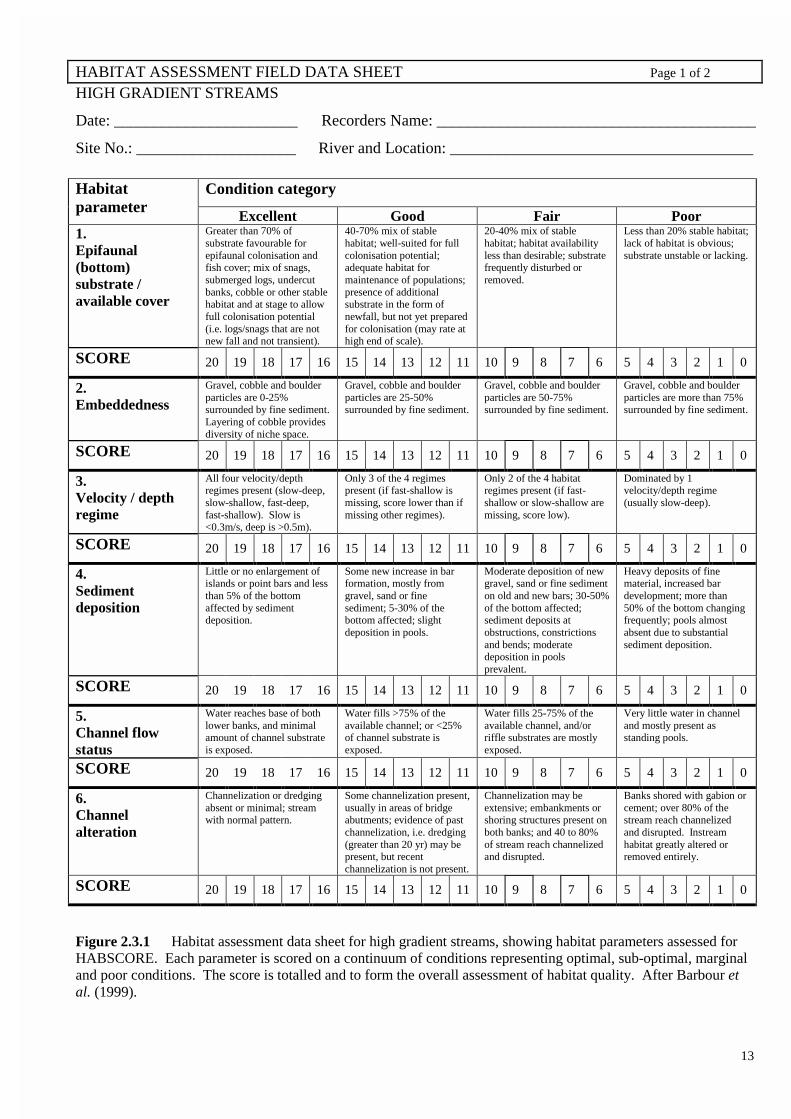
et al., 1999). HABSCORE is composed of ten habitat parameters (Figure 2.3.1). To

reflect the difference in habitat types between upland and lowland streams, separate

assessments have been developed for high and low gradient conditions (Barbour et al.,

1999). At each site, individual parameters are assessed and rated according to a

continuum of scores that represent optimal, sub-optimal, marginal or poor condition

(Figure 2.3.1). A total score is obtained for each site, and is subsequently used to

determine the percent comparability to reference conditions (Plafkin et al., 1989).

However, the individual parameter scores and the total assessment score also provide an

overall assessment of habitat condition at the sampling site.

13

HABITAT ASSESSMENT FIELD DATA SHEET Page 1 of 2

HIGH GRADIENT STREAMS

Date: _______________________ Recorders Name: ________________________________________

Site No.: ____________________ River and Location: ______________________________________

Condition categoryHabitatparameter

Excellent Good Fair Poor1.Epifaunal(bottom)substrate /available cover

Greater than 70% ofsubstrate favourable forepifaunal colonisation andfish cover; mix of snags,submerged logs, undercutbanks, cobble or other stablehabitat and at stage to allowfull colonisation potential(i.e. logs/snags that are notnew fall and not transient).

40-70% mix of stablehabitat; well-suited for fullcolonisation potential;adequate habitat formaintenance of populations;presence of additionalsubstrate in the form ofnewfall, but not yet preparedfor colonisation (may rate athigh end of scale).

20-40% mix of stablehabitat; habitat availabilityless than desirable; substratefrequently disturbed orremoved.

Less than 20% stable habitat;lack of habitat is obvious;substrate unstable or lacking.

SCORE 20 19 18 17 16 15 14 13 12 11 10 9 8 7 6 5 4 3 2 1 0

2.Embeddedness

Gravel, cobble and boulderparticles are 0-25%surrounded by fine sediment.Layering of cobble providesdiversity of niche space.

Gravel, cobble and boulderparticles are 25-50%surrounded by fine sediment.

Gravel, cobble and boulderparticles are 50-75%surrounded by fine sediment.

Gravel, cobble and boulderparticles are more than 75%surrounded by fine sediment.

SCORE 20 19 18 17 16 15 14 13 12 11 10 9 8 7 6 5 4 3 2 1 0

3.Velocity / depthregime

All four velocity/depthregimes present (slow-deep,slow-shallow, fast-deep,fast-shallow). Slow is<0.3m/s, deep is >0.5m).

Only 3 of the 4 regimespresent (if fast-shallow ismissing, score lower than ifmissing other regimes).

Only 2 of the 4 habitatregimes present (if fast-shallow or slow-shallow aremissing, score low).

Dominated by 1velocity/depth regime(usually slow-deep).

SCORE 20 19 18 17 16 15 14 13 12 11 10 9 8 7 6 5 4 3 2 1 0

4.Sedimentdeposition

Little or no enlargement ofislands or point bars and lessthan 5% of the bottomaffected by sedimentdeposition.

Some new increase in barformation, mostly fromgravel, sand or finesediment; 5-30% of thebottom affected; slightdeposition in pools.

Moderate deposition of newgravel, sand or fine sedimenton old and new bars; 30-50%of the bottom affected;sediment deposits atobstructions, constrictionsand bends; moderatedeposition in poolsprevalent.

Heavy deposits of finematerial, increased bardevelopment; more than50% of the bottom changingfrequently; pools almostabsent due to substantialsediment deposition.

SCORE 20 19 18 17 16 15 14 13 12 11 10 9 8 7 6 5 4 3 2 1 0

5.Channel flowstatus

Water reaches base of bothlower banks, and minimalamount of channel substrateis exposed.

Water fills >75% of theavailable channel; or <25%of channel substrate isexposed.

Water fills 25-75% of theavailable channel, and/orriffle substrates are mostlyexposed.

Very little water in channeland mostly present asstanding pools.

SCORE 20 19 18 17 16 15 14 13 12 11 10 9 8 7 6 5 4 3 2 1 0

6.Channelalteration

Channelization or dredgingabsent or minimal; streamwith normal pattern.

Some channelization present,usually in areas of bridgeabutments; evidence of pastchannelization, i.e. dredging(greater than 20 yr) may bepresent, but recentchannelization is not present.

Channelization may beextensive; embankments orshoring structures present onboth banks; and 40 to 80%of stream reach channelizedand disrupted.

Banks shored with gabion orcement; over 80% of thestream reach channelizedand disrupted. Instreamhabitat greatly altered orremoved entirely.

SCORE 20 19 18 17 16 15 14 13 12 11 10 9 8 7 6 5 4 3 2 1 0

Figure 2.3.1 Habitat assessment data sheet for high gradient streams, showing habitat parameters assessed forHABSCORE. Each parameter is scored on a continuum of conditions representing optimal, sub-optimal, marginaland poor conditions. The score is totalled and to form the overall assessment of habitat quality. After Barbour etal. (1999).

14

HABITAT ASSESSMENT FIELD DATA SHEET Page 2 of 2

HIGH GRADIENT STREAMS

Date: _______________________ Recorders Name: ________________________________________

Site No.: ____________________ River and Location: ______________________________________

Condition categoryHabitatparameter

Excellent Good Fair Poor7.Frequency ofriffles (or bends)

Occurrence of rifflesrelatively frequent; ratio ofdistance between rifflesdivided by width of thestream <7:1 (generally 5 to7); variety of habitat is key.In streams where riffles arecontinuous, placement ofboulders or other large,natural obstruction isimportant.

Occurrence of rifflesinfrequent; distance betweenriffles divided by the widthof the stream is between 7 to15.

Occasional riffle or bend;bottom contours providesome habitat; distancebetween riffles divided bythe width of the stream isbetween 15 to 25.

Generally all flat water orshallow riffles; poor habitat;distance between rifflesdivided by the width of thestream is a ratio of >25.

SCORE 20 19 18 17 16 15 14 13 12 11 10 9 8 7 6 5 4 3 2 1 0

8.Bank stability(score each bank)

Banks stable; evidence oferosion or bank failureabsent or minimal; littlepotential for futureproblems. <5% of bankaffected.

Moderately stable;infrequent, small areas oferosion mostly healed over.5-30% of bank in reach hasareas of erosion.

Moderately unstable; 30-60% of bank in reach hasareas of erosion; higherosion potential duringfloods.

Unstable; many erodedareas; 'raw' areas frequentalong straight sections andbends; obvious banksloughing; 60-100% of bankhas erosional scars.

SCORE Left bank 10 9 8 7 6 5 4 3 2 1 0

SCORE Right bank 10 9 8 7 6 5 4 3 2 1 0

9.Vegetativeprotection(score each bank)

More than 90% of thestreambank surfaces andimmediate riparian zonecovered by nativevegetation, including trees,understorey shrubs, or nonwoody macrophytes;vegetative disruptionthrough grazing or mowingminimal or not evident;almost all plants allowed togrow naturally.

70-90% of the streambanksurfaces covered by nativevegetation, but one class ofplants is not well-represented; disruptionevident but not affecting fullplant growth potential to anygreat extent; more than onehalf of the potential plantstubble height remaining.

50-70% of the streambanksurfaces covered byvegetation; disruptionobvious; patches of bare soilor closely croppedvegetation common; lessthan one-half of the potentialplant stubble heightremaining.

Less than 50% of thestreambank surfaces coveredby vegetation; disruption ofstreambank vegetation isvery high; vegetation hasbeen removed to 5centimetres or less inaverage stubble height.

SCORE Left bank 10 9 8 7 6 5 4 3 2 1 0

SCORE Right bank 10 9 8 7 6 5 4 3 2 1 0

10.Riparian zonescore(score each bank)

Width of riparian zone >18metres; human activities (i.e.roads, lawns, crops etc.)have not impacted theriparian zone.

Width of riparian zone 12-18metres; human activitieshave impacted riparian zoneonly minimally.

Width of riparian zone 6-12metres; human activitieshave impacted zone a greatdeal.

Width of riparian zone <6metres; little or no riparianvegetation is present becauseof human activities.

SCORE Left bank 10 9 8 7 6 5 4 3 2 1 0

SCORE Right bank 10 9 8 7 6 5 4 3 2 1 0

TOTAL HABITAT SCORE _________________

Figure 2.3.1 (cont.)

15

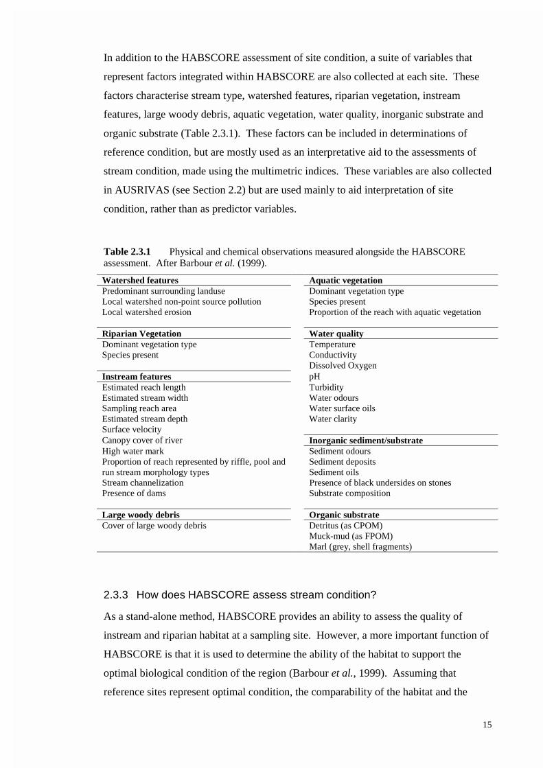
In addition to the HABSCORE assessment of site condition, a suite of variables that

represent factors integrated within HABSCORE are also collected at each site. These

factors characterise stream type, watershed features, riparian vegetation, instream

features, large woody debris, aquatic vegetation, water quality, inorganic substrate and

organic substrate (Table 2.3.1). These factors can be included in determinations of

reference condition, but are mostly used as an interpretative aid to the assessments of

stream condition, made using the multimetric indices. These variables are also collected

in AUSRIVAS (see Section 2.2) but are used mainly to aid interpretation of site

condition, rather than as predictor variables.

Table 2.3.1 Physical and chemical observations measured alongside the HABSCOREassessment. After Barbour et al. (1999).

Watershed features Aquatic vegetationPredominant surrounding landuse Dominant vegetation typeLocal watershed non-point source pollution Species presentLocal watershed erosion Proportion of the reach with aquatic vegetation

Riparian Vegetation Water qualityDominant vegetation type TemperatureSpecies present Conductivity

Dissolved OxygenInstream features pHEstimated reach length TurbidityEstimated stream width Water odoursSampling reach area Water surface oilsEstimated stream depth Water claritySurface velocityCanopy cover of river Inorganic sediment/substrateHigh water mark Sediment odoursProportion of reach represented by riffle, pool andrun stream morphology types

Sediment depositsSediment oils

Stream channelization Presence of black undersides on stonesPresence of dams Substrate composition

Large woody debris Organic substrateCover of large woody debris Detritus (as CPOM)

Muck-mud (as FPOM)Marl (grey, shell fragments)

2.3.3 How does HABSCORE assess stream condition?

As a stand-alone method, HABSCORE provides an ability to assess the quality of

instream and riparian habitat at a sampling site. However, a more important function of

HABSCORE is that it is used to determine the ability of the habitat to support the

optimal biological condition of the region (Barbour et al., 1999). Assuming that

reference sites represent optimal condition, the comparability of the habitat and the

16

biota to this reference state can be plotted to determine the ability of the habitat to

support the biological community (Figure 2.3.2). There are three important aspects of

Figure 2.3.2:

• the upper right hand corner represents a situation with good habitat quality and

good biological condition;

• the mid-section of the curve represents a situation where habitat quality

decreases and the biological community responds with a concomitant decrease;

and,

• the lower left hand corner represents a situation where habitat quality is poor and

unable to support the biological community (Barbour, 1991).

Apart from the three situations outlined above, comparison of the condition of the biota

with the condition of the habitat can also highlight situations of potential water quality

degradation, where habitat quality is high but biological condition is poor (Barbour et

al., 1999).

Habitat quality is the initial focus of the Rapid Bioassessment Protocols. Habitat

quality at the reference sites is compared against habitat quality at the test site and if

equivalent, then a direct comparison of the biological condition can be made using the

biological metrics (Plafkin et al., 1989). This ensures that assessments of biological

condition indicate impairment, rather than inherent natural differences in stream habitat.

If habitat quality is lower at a test site than at the reference sites, then the ability of the

habitat to support biota is investigated as a first step, before a determination of

biological condition is made (Plafkin et al., 1989).

2.3.4 How does HABSCORE link physical and chemical features with the

biota?

HABSCORE was designed to complement assessments of biological condition made

using the rapid biological assessment protocols. This compatibility is based on the

assumption that the quality and quantity of available physical habitat has a direct

influence on biotic communities (Maddock 1999; Rankin, 1995). The parameters

measured in HABSCORE (Figure 2.3.1) represent aspects of the habitat that are related

to aquatic life use and which are a potential source of limitation to the aquatic biota

(Barbour, 1991; Barbour et al., 1999). Thus, the empirical links between habitat and the

biota are reflected in this relationship. The process used to determine the ability of the

17

habitat to support an optimal biological community (see Section 2.3.3) also captures

these empirical links by considering habitat quality to be a templet that influences the

types of biotic communities that can potentially be attained under certain conditions.

Figure 2.3.2 The relationship between habitat and biological condition. Re-drawn fromBarbour (1991).

2.4 Index of Stream Condition

2.4.1 How did the Index of Stream Condition come about?

Australian Governments are increasing their focus on rivers via legislative, research and

rehabilitation actions (Ladson et al., 1999). Within this environment, the Victorian

Index of Stream Condition (ISC) was developed in response to a managerial need to

'use indicators to track aspects of environmental condition and provide managerially or

scientifically useful information' (Ladson et al., 1999, p454).

The ISC evolved in four stages. Stage 1 involved the development of the concept and

included a review of stream assessment methods, input from stream scientists and

managers, and development of an ISC prototype (Ladson and White, 1999). The

desired attributes considered in development of the ISC concept were:

Comparable

0

10SupportingPartially

Supporting

Moderately impaired

Slightly impaired

Nonimpaired

10090807060504030200 10Habitat Quality (% of Reference)

Severely impairedNonsupporting

Bio

logi

cal C

ondi

tion

(% o

f re

fere

nce)

20

40

30

50

60

70

80

100

90

18

• the indicators are key components of stream condition;

• the methodology is founded in science;

• the results are accessible to managers;

• data collection methods are objective and repeatable;

• natural variability is considered;

• application is cost effective; and,

• indicators are sensitive to management intervention (Ladson and White, 1999).

Stage 1 is analogous to the aims of the current Physical and Chemical Assessment

Module. Stages 2 and 3 of the ISC involved trialing and refining the concept and Stage

4 involved application of the ISC across Victoria (Ladson and White, 1999). Future

stages will involve assessment and further refinement of the method (Ladson and White,

1999).

2.4.2 How does the Index of Stream Condition work?

The ISC measures stream condition within reaches that are between 10 and 30km in

length (Ladson and White, 1999). Reaches are defined as 'contiguous sections of stream

chosen so that they are approximately homogeneous in terms of the five components of

stream condition' (Ladson et al., 1999 p456). Reaches are delineated mainly from

1:250 000 topographic maps or aerial photographs. Within each reach, measurement

sites are selected on the basis of:

• the representativeness of each site to reach characteristics;

• proximity to existing biological, physical and water quality monitoring sites;

and,

• accessibility for sampling purposes (DNRE, 1997).

The ISC consists of five sub-indices, which represent key components of stream

condition (Table 2.4.1). Each sub-index consists of indicators, which are calculated

using data collected in the field or by desk based methods. Each indicator is then

assigned a rating score (see Section 2.4.3). Sub-index scores are calculated by summing

the component indicator scores, and the overall ISC score is calculated by summing the

sub-index scores (Ladson et al., 1999).

19

Table 2.4.1 List of indicators used in the Index of Stream Condition. After Ladson andWhite (1999) and Ladson et al. (1999).

Sub-index Basis for sub-index value Indicators within sub-index

Hydrology Comparison of the current flowregime with the flow

Amended annual proportionalflow deviation

regime existing under naturalconditions

Daily flow variation due tochange of catchment permeabilityDaily flow variation due topeaking hydroelectricity stations

Physical Form Assessment of channel Bank stabilitystability and amount of Bed stabilityphysical habitat Impact of artificial barriers on fish

migrationInstream physical habitat

Streamside Zone Assessment of quality and Width of streamside zonequantity of streamside Longitudinal continuityvegetation Structural intactness

Cover of exotic vegetationRegeneration of indigenouswoody vegetationBillabong condition

Water Quality Assessment of key water Total phosphorusquality parameters Turbidity

Electrical conductivityAlkalinity / acidity

Aquatic Life Presence of SIGNALmacroinvertebrate families AUSRIVAS

2.4.3 How does the Index of Stream Condition assess stream condition?

The ISC uses a rating system to assess stream condition. The use of a rating system is

designed to provide as much resolution as possible, within the constraint that there is

'limited knowledge of the relationship between a change in the indicator and

environmental effects' (Ladson and White, 1999, p10). Values for each indicator are

assigned a rating on the basis of comparison with a reference state (Figure 2.4.1). These

ratings are summed to produce an overall score that reflects a continuum of stream

conditions from excellent to very poor (Figure 2.4.1). In calculating the overall ISC

scores, the scores for each sub-index and for each indicator can be weighted, depending

on the perceived importance of each, or the availability of data (Ladson and White,

1999).

The ISC is based on the premise that the hydrology, physical form, streamside zone,

water quality and aquatic life components indicate the processes and functions that act

to influence stream condition. For example, the hydrology sub-index reflects deviation

20

of the current flow regime from natural conditions, the physical form sub-index reflects

channel morphology and the provision of biotic habitat, and the streamside zone sub-

index reflects the importance of riparian zone and floodplain processes (Ladson and

White, 1999; Ladson et al., 1999). A holistic assessment of stream condition is

achieved by integrating these components into a single ISC score. However, it is

IndicatorRating

Corresponding reference category Example values:pH range

4 Very close to reference state 6.5 - 7.5

3 Minor modification from reference state 6.0 - < 6.5 or 7.5 – 8.0

2 Moderate modification from reference state 5.5 - < 6.0 or 8.0 – 8.5

1 Major modification from reference state 4.5 - < 5.5 or 8.5 – 9.5

0 Extreme modification from reference state <4.5 or > 9.5

Overall ISC score Stream condition

45 - 50 Excellent

35 - 44 Good

25 - 34 Marginal

15 - 24 Poor

< 14 Very poor

Figure 2.4.1 Assessment of stream condition using the Index of Stream Condition. Derivedfrom Ladson and White (1999).

Ratings are summed withineach sub-index, then sub-indexscores are summed to produce

an overall ISC score.

Repeated for eachindicator. Reference

ranges are derived fromexisting literature.

1. Calculate ratings for indicators

2. Calculate ISC score

21

recommended that the scores for the component sub-indices are reported alongside the

overall ISC score, because the overall score may be composed of sub-indices that vary

in condition (Ladson and White, 1999).

The ISC was designed to provide an assessment of long term changes in the

environmental condition of rural stream reaches 10-30km in length, with surveys

conducted at five year intervals (Ladson and White, 1999). As such, the 'level of detail

is only sufficient to signal potential problems, suggest their cause and highlight aspects

that may need specific investigations' (Ladson et al., 1999, p455). However, the ISC is

a tool for determining the success of environmental intervention policies (Ladson and

White, 2000) and can be used in a management context to:

• benchmark stream condition, and for reporting to local, regional, state or

Commonwealth agencies;

• aid objective setting by, and provide feedback to, natural resource managers

(particularly Catchment Management Authorities) and in particular, to assess

trade-offs between utilitarian demands on streams and environmental condition;

• judge the effectiveness of intervention, in the long-term, in managing and

rehabilitating stream condition; and,

• review performance against expected outcomes (Ladson and White, 1999).

2.4.4 How does the Index of Stream Condition link physical and chemical

features with the biota?

The ISC is designed to be a broad scale and long term assessment. As such, the ISC

consists of five sub-indices that reflect different components of stream condition. The

aquatic life sub-index is the component that reflects overall biotic condition within the

sampling reach (Ladson and White, 1999). Macroinvertebrate indicators are used in the

ISC, because this group of organisms provides a continuous assessment of the

environment which they inhabit (Rosenberg and Resh, 1993; Ladson and White, 1999).

As such, the aquatic life sub-index is inherently related to the hydrology, physical form,

streamside zone and water quality sub-indices (Ladson and White, 1999). Inclusion of

the aquatic life sub-index provides a somewhat independent measure of stream

condition, and can be particularly useful in situations where the biota are degraded but

the physical, chemical and hydrological indices are not (Ladson and White, 1999).

While there is empirical evidence that broadly links degradation in physical, chemical

22

and hydrological factors with degradation in macroinvertebrate communities, care must

be taken when comparing scores for the aquatic life sub-index with scores for the other

sub-indices. This is because a scoring system may not be a sensitive reflection of

mechanistic relationships between environmental factors and macroinvertebrate

community composition.

2.5 Geomorphic River Styles

2.5.1 How did Geomorphic River Styles come about?

River health has traditionally been viewed from a biological perspective, because

'effects on biota are usually the final point of environmental degradation and pollution

of rivers' (Norris and Thoms, 1999, p197). However, there is an inherent link between

the potential health of biota, and the availability of physical habitat (Brierley et al.,

1999). As such, assessment of river health from a biological perspective cannot proceed

effectively when analysed in isolation from the factors that determine river structure and

function. Geomorphic River Styles aims to address the physical structure and function

components of river health. It is framed around 'direct linkage of vegetative and

geomorphic process, providing an assessment of habitat availability along river courses,

and hence indirect linkage to river ecology' (Brierley et al., 1996, p2).

Assessment of stream condition from a distinctly geomorphological perspective has

many benefits to river managers, including:

• an ability to characterise and explain river behaviour at different positions within

catchments;

• provision of a predictive basis to assess future river character and responses to

disturbance;

• provision of a basis to determine suitable river structures to support viable

habitats along river courses;

• help to develop pro-active, rather than reactive, management strategies, setting

realistic target goals in development of River/Catchment Management Plans and

more effectively prioritorising allocation to management issues; and,

• an ability to be used in programs to assess and monitor river condition (Brierley

et al., 1996).

23

2.5.2 How does Geomorphic River Styles work?

Geomorphic River Styles is a procedure that provides 'a baseline survey of river

character and behaviour, evaluating the physical controls on river structure at differing

positions in catchments' (Brierley et al., 1996, p2). The procedure is set within a nested

hierarchical framework (Frissell et al., 1986) and as such, it incorporates assessment of

river structure at the catchment, reach and geomorphic unit scales (Brierley et al.,

1996).

There are five stages in the assessment of river character and behaviour:

1. Data compilation (description and mapping)

2. Data analysis (explanation of river character and behaviour)

3. Prediction of future likely river structure

4. Prioritorisation of catchment management issues

5. Identification of suitable river structures for Rivercare planning (Brierley et al.,

1996).

Stage one comprises both pre-field data collection and field data collection (Brierley et

al., 1996). During the pre-field data collection component, catchment scale

characteristics are measured off maps, or by using GIS capabilities (Table 2.5.1).

Consideration is also given to historical and archival information about the catchment.

In addition, the pre-field component involves identification of reach boundaries off

1:12000 air photographs and a range of reach scale characteristics is subsequently

measured at each reach (Table 2.5.1). The reaches delineated off maps are used as

sampling units in the field data collection component (Brierley et al., 1996), although

the reaches are ratified in the field prior to data collection. Geomorphic units are

identified within each reach and at representative locations, the characteristics of each

geomorphic unit are recorded (Table 2.5.1). A detailed sediment analysis is also

conducted in each geomorphic unit (Table 2.5.1).

In Stage two, data collected in the pre-field and field components are used to interpret

river behaviour. This process involves several steps and follows the hierarchical

framework. Firstly, the assemblage of geomorphic units is assessed, to

24

Table 2.5.1 Catchment, reach and geomorphic unit characteristics measured in theGeomorphic River Styles method. After Brierley et al. (1996).

CATCHMENT CHARACTERISTICS GEOMORPHIC UNIT CHARACTERISTICSRelief measures IdentificationCatchment relief Within channel unitsCatchment relief ratio Channel marginal units and bank characterLongitudinal profile Floodplain unitsValley side slope length and angle Morphology and dimensions of geomorphic unitsAreal properties Shape and sizeCatchment area Channel geometryDrainage pattern Channel bed elevationElongation ratio Width to depth ratioDrainage density Hydraulic parametersLinear measurements Flow characterStream order Mannings roughness coefficient (n)Stream length Froude numberOther measures Vegetation characterGeology Vegetation cover dimensionsAverage annual rainfall and monthly averages Vegetation compositionLanduseVegetation distribution and type

Assemblage and connectivity of geomorphic units throughout the reach

Discharge Spatial character of geomorphic unitsChannel – floodplain relationship

REACH CHARACTERISTICS Lateral stability of the channelChannel planform Degree and character of channel obstructionPlanform geometry Stream powerRadius of channel curvature to mean channelwidth ratio (rc/w)

Bankfull dischargeSediment attributes

Meander wavelength Grain size and distributionType of geomorphic units present SortingConfinement RoundingValley width Facies / sedimentary structuresDegree and character of channel constriction Sediment mix and degree of packingTerrace character Type of gradingVegetation character Sediment relationsPercent coverage Degree of sediment storage

Sediment yield or sediment delivery ratio (SDR)

provide insight into the formative processes within a reach (Brierley et al., 1996).

Examples of some of the links between geomorphic units and formative processes that

can be deduced from this stage are:

• lateral and/or downstream migration of a channel is reflected by point bar

sedimentation, channel asymmetry, eroding concave banks, ridge and swale

floodplain topography, meander cutoffs etc.;

• channel contraction is reflected by bench formation and in-channel

sedimentation;

• bedrock confinement is reflected by differing assemblages of geomorphic units,

dependent on valley alignment, such as concave bank benches, channel scour or

steep levee-flood channel assemblages;

• channel avulsion is recorded by abandoned channels on the floodplain;

25

• sand sheet deposition on floodplains may record changes in the pattern of

sedimentation; and,

• a sediment-choked channel, with dissected bars, may reflect bed aggradation

(Brierley et al., 1996).

In the second interpretation step, reaches are amalgamated to form source, transfer,

throughput and accumulation zones, based on the assemblage of geomorphic units and

associated sediment relations along reaches. These 'process zones' represent the

capacity of the stream to temporarily store and accumulate materials (Brierley et al.,

1996). Thirdly, the catchment characteristics are used to determine the nature of the

controls on river character and behaviour in each process zone (Brierley et al., 1996).

The evolution of the river is then assessed in a historical context, and provides an

indication of pre-disturbance stream characteristics. Lastly, the 'direct controls on

habitat availability are assessed by analysis of changes to channel geometry and

planform, the assemblage of geomorphic units within each process zone and the nature

of altered associations that each of these geomorphic features have with riparian

vegetation' (Brierley et al., 1996, p26).

2.5.3 How does Geomorphic River Styles assess stream condition?

The assessment of stream condition using Geomorphic River Styles is achieved using

two approaches: comparison of contemporary stream character and behaviour with the

conditions expected in undisturbed conditions; and prediction of future river character

and behaviour based on extrapolation from contemporary behaviour, sediment storage,

and/or theoretical notions of river behaviour (Brierley et al., 1996; Fryirs et al., 1996).

The focus of both approaches is the behaviour of process zones, because each zone type

may respond differently to disturbance and result in a particular assemblage of

geomorphic units.

In the first approach, comparison of contemporary stream conditions with undisturbed

conditions allows analysis of changes in both planform (Figure 2.5.1) and cross

sectional (Figure 2.5.2) channel structure within different process zones. For example,

in the Wolumla Creek Catchment on the South Coast of New South Wales (figure 2.5.1

and fiure 2.5.2), river channel changes since human settlement of the area can be

summarised as follows:

26

• channel planform and geometry have become better defined;

• the association of geomorphic units is more homogeneous despite a larger range

of geomorphic units being present;

• variability in the sedimentary character of geomorphic units has been reduced;

• vegetation associations have decreased in variability and are now more

homogeneous;

• longitudinal connectivity has increased throughout the catchment. Lateral

channel floodplain connectivity has decreased;

• organic matter and nutrient retention within-catchment has greatly decreased;

and,

• hydrological implications have been transformed largely as a result of the calibre

and volume of materials stored within the channel (Fryirs et al., 1996).

In the second approach to assessment of stream condition, prediction of likely future

behaviour is made by extrapolation from contemporary behaviour, sediment storage

(Figure 2.5.3) and relationships with theoretical notions of river behaviour (Figure

2.5.4) (Fryirs et al., 1996). For example, in the Wolumla Catchment, analysis based on

sediment storage identified sites which were most sensitive to future sediment release

(Figure 2.5.3) (Fryirs et al., 1996). Analysis based on theoretical river behaviour can

identify the predictive relationships between variables related to river behaviour and

channel geometry (Figure 2.5.4), which in turn, can be used to assist in setting targets

for stream restoration or Rivercare programs. However, in the Wolumla Catchment, the

classical notions of river behaviour do not apply (Fryirs et al., 1996). In addition, the

ability of variables to predict channel geometry was highly variable among sub-

catchments, highlighting the need for analysis of predictive relationships at the scale of

sub-catchments (Fryirs et al., 1996).

2.5.4 How does Geomorphic River Styles link physical and chemical features

with the biota?

Geomorphic River Styles is a geomorphological stream assessment method that relies

heavily on sedimentary characteristics. As such, it does not directly measure the biota.

27

Figure 2.5.1 Planform view of pre-disturbance (left) and post-disturbance (right) channelcharacter within upland, mid-catchment and lowland zones of the Wolumla Creek catchment.After Fryirs et al. (1996).

28

Figure 2.5.2 Cross-sectional view of pre-disturbance (left) and post-disturbance (right)channel character within upland, mid-catchment and lowland zones of the Wolumla Creekcatchment. After Fryirs et al. (1996).

29

Figure 2.5.3 Identification of sensitive sites in the Wolumla Catchment, based on sedimentstorage. Frogs Hollow Swamp and Frogs Hollow floodout are intact features which if incisedcould supply significant volumes of material. Wolumla and South Wolumla valley fill sourcezones have had the majority of their fills removed, but a significant volume of material stillremains stored within these zones. Greendale channel expansion site is an actively erodingtransfer zone which is still supplying significant volumes of sediment to Frogs Hollow Creekand is the most sensitive site in the catchment. After Fryirs et al. (1996).

30 Figure 2.5.4 Predictive relationships between stream characteristics in sub-catchments of the Wolumla Catchment. After Fryirs et al. (1996).

31

However, the process of deducing and predicting geomorphic stream characteristics and

behaviour is essentially equivalent to deducing and predicting habitat availability

because 'geomorphic processes determine the structure, or physical template, of a river

system' (Brierley et al., 1999, p840; see also Cohen et al., 1996). In turn, this template

provides the 'framework upon which a wide range of biophysical processes interact'

(Brierley et al., 1999, p840; see also Resh et al., 1994; Townsend and Hildrew, 1994).

Thus, Geomorphic River Styles may have the potential to merge geomorphology and

ecology together under the common banner of a physical habitat template.

The implications of geomorphic channel changes for riverine ecology are evaluated by

considering lateral and longitudinal connectivity of the river system, the hydrological

regime, and the processing and storage of nutrients and organic matter (Brierley et al.,

1996). In the Wolumla Catchment, some of the effects of channel behaviour on riverine

ecology are reported as:

• changes in sediment character in the lowland and mid-catchment reaches has

resulted in a reduction in the variability of substrate distribution throughout the

reaches;

• there has been alteration to the longitudinal connectivity through a significant

reduction in riparian vegetation. This has important implications for detritus

inputs to stream ecosystems, nutrient retention and the micro-climate of streams,

as well as having a possible impact on detritivores;

• reduction in riparian vegetation has resulted in the dominance of exotic species;

• the change in geomorphic character of process zones have altered the

relationship between sources of organic matter, retention and redistribution of

this material;

• the changes in channel form of process zones associated with large scale bed

aggradation could also have significant impacts on the hyporheic zone; and,

• changes to longitudinal relationships of stream ecosystems may result in

disjointed migration pathways and reduced habitats for certain fish species

(Cohen et al., 1996).

Despite the potential for Geomorphic River Styles to assess biotic habitat, there has

been no direct testing of the relationships between different types of biota and different

geomorphic units, or process zones. The view of what constitutes a functional habitat

may differ significantly between the geomorphological and the biological perspective.

32

For instance, is the distribution of macroinvertebrate communities within a catchment

related to the distribution of source, input, throughput and accumulation zones within a

catchment? If certain assemblages of geomorphic units are characteristic of process

zones, do macroinvertebrate communities recognise and differentiate between these

geomorphic units? Determination of these relationships through future research would

provide a strong foundation for linking biotic condition with habitat condition, within a

geomorphic process framework.

2.6 State of the Rivers Survey

2.6.1 How did the State of the Rivers Survey come about?

The State of the Rivers Survey was developed in Queensland, in response to a need for

detailed information on the physical and environmental condition of streams and rivers

(Anderson, 1993a). This information would then be available to the Queensland

Department of Primary Industries (DPI) for use in the Integrated Catchment

Management process (Anderson, 1993a). The State of the Rivers Survey is not

designed to establish the trend or rate of change of stream condition, but rather, it

provides a 'snapshot' of the physical and environmental condition of streams. These

data can then be used to:

• provide an objective and comprehensive benchmark against which future trends

and rates of change of conditions can be assessed by conducting follow-up

surveys;

• provide the fundamental information required to classify rivers and streams; and,

• provides an overview to help identify resource management and utilisation

practices contributing to the deterioration in physical and ecological condition of

rivers (Anderson, 1993a).

The State of the Rivers Survey was developed in two stages. The first stage involved

development (Anderson, 1993a; Anderson, 1993b) and testing (Anderson, 1993c) of the

method. The State of the Rivers Survey has subsequently been applied to assess stream

condition in 26 catchments in New South Wales and Queensland (Anderson, 1999).

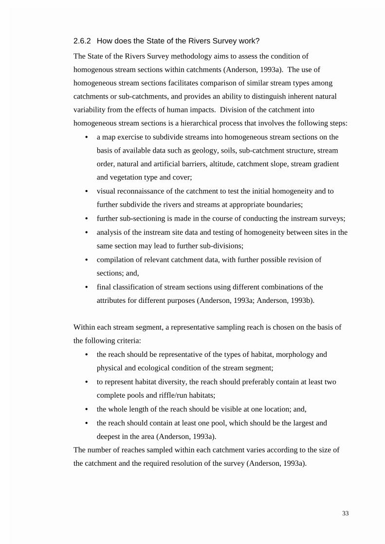
33

2.6.2 How does the State of the Rivers Survey work?

The State of the Rivers Survey methodology aims to assess the condition of

homogenous stream sections within catchments (Anderson, 1993a). The use of

homogeneous stream sections facilitates comparison of similar stream types among

catchments or sub-catchments, and provides an ability to distinguish inherent natural

variability from the effects of human impacts. Division of the catchment into

homogeneous stream sections is a hierarchical process that involves the following steps:

• a map exercise to subdivide streams into homogeneous stream sections on the

basis of available data such as geology, soils, sub-catchment structure, stream

order, natural and artificial barriers, altitude, catchment slope, stream gradient

and vegetation type and cover;

• visual reconnaissance of the catchment to test the initial homogeneity and to

further subdivide the rivers and streams at appropriate boundaries;

• further sub-sectioning is made in the course of conducting the instream surveys;

• analysis of the instream site data and testing of homogeneity between sites in the

same section may lead to further sub-divisions;

• compilation of relevant catchment data, with further possible revision of

sections; and,

• final classification of stream sections using different combinations of the

attributes for different purposes (Anderson, 1993a; Anderson, 1993b).

Within each stream segment, a representative sampling reach is chosen on the basis of

the following criteria:

• the reach should be representative of the types of habitat, morphology and

physical and ecological condition of the stream segment;

• to represent habitat diversity, the reach should preferably contain at least two

complete pools and riffle/run habitats;

• the whole length of the reach should be visible at one location; and,

• the reach should contain at least one pool, which should be the largest and

deepest in the area (Anderson, 1993a).

The number of reaches sampled within each catchment varies according to the size of

the catchment and the required resolution of the survey (Anderson, 1993a).

34

Table 2.6.1 Data components and types of variables measured in the State of the RiversSurvey. Compiled from the detailed survey data sheets provided in Anderson (1993b).

Sub-section elements1 Bank conditionSection boundaries Bank stability6

Sub-catchment centroid Bank slope6

Elevation information Bank shape6

Overall bank condition6

Hydrology2 Factors affecting stabilityWater flow Artificial bank protection measuresTime since last runoff Levee banksGeneral local conditionsInstream water quality measurements3 Bed and bar condition

Bar type and distributionSite description Bar sizeGrid reference Gravel angularity and shapeLatitude Gravel surface characteristicsLongitude Bed compactionCatchment area Factors affecting stabilityAltitude Controls stabilising the bedMap details Passage for fish and other organismsSite access details Overall bed stability ratingPhotograph details

VegetationReach environs – temporal and spatial Width of riparian zone6

Water level at sampling time Vegetation cover of plant types6

Channel pattern Percent exotic species in riparian zone6

Local land use Local species checklist6

Local disturbance Aquatic vegetation – submerged and floatingLocal vegetation types Emergent aquatic vegetationFloodplain featuresLocal land tenure Aquatic habitatOverall disturbance rating Instream debris cover

Canopy cover6

Channel habitat Vegetation overhang6

Channel habitat types Root overhang6

Reach length Bank overhang6

Sketch of reach Man-made overhang6

Overall site rating for all aquatic lifeCross-sections4

Depth5 Scenic, recreational and conservation valuesWater velocity5 Recreational opportunity typeBed sediments5 Recreation types suitable for the areaBank dimensions Scenic value assessmentBank sediments Initial conservation value assessment

1. This component is usually completed post-survey, to characterise the final homogeneous stream sections2. This component is desk based and is designed to establish an interface with hydrological and water quality

data through HYDSYS3. Measurement of depth, water temperature, dissolved oxygen, pH, conductivity, salinity, turbidity, secchi

depth and water velocity is optional4. One cross section is measured in each habitat type present within a reach5. Measured at up to 15 locations within the cross sectional transect6. Measured for left and right banks

In addition to the map-based data that are used to delineate the initial stream sections,

the State of the Rivers Survey consists of 11 data components (Table 2.6.1) that are

collected at each representative sampling reach. Each data component is composed of

different types of variables that represent the physical and environmental aspects of the

35

stream channel (Table 2.6.1). Variables are generally measured using visual estimation,

but some variables require physical measurement or an interpretive rating of condition.

2.6.3 How does the State of the Rivers Survey assess stream condition?

The basis for assessment of stream condition in the State of the Rivers Survey is 'the

extent to which the values or perceived function of an attribute has declined from a

pristine or undisturbed condition' (Anderson, 1999). A series of condition ratings are

produced for each data component. Formulas are used to derive condition ratings, using

subsets of variables collected within each component (Anderson 1993b). These

condition ratings are based on the extent of degradation from a theoretical maximum of

100%, where 100% percent represents the full value, pristine condition or complete

function for the component and 0% represents a complete loss of these (Anderson,

1999). Comparisons with representative sites in good condition are also used to scale

the ratings (Anderson, 1999).

Using the condition ratings for each data component, an assessment of condition is

derived for each homogeneous stream section (Figure 2.6.1). A final assessment of

stream condition within a catchment is achieved by calculating the number of

homogeneous stream sections that correspond to each condition rating, for each data

component (Figure 2.6.1). The length of stream within each catchment that corresponds

to a certain condition can also be calculated (Figure 2.6.1). In addition, an overall

condition rating can also be calculated for the whole catchment by resetting the

condition ratings for all the data components combined (Anderson, 1993c). Thus,

stream condition can be reported on several levels of resolution that can encompass

combinations of individual data components or all data components together, as well as

individual stream sections or the entire catchment.

2.6.4 How does the State of the Rivers Survey link physical and chemical

features with the biota?

The State of the Rivers Survey was designed to 'estimate the ecological condition [of

rivers] in terms of the condition of the instream habitat, rather than by conducting flora

or faunal surveys' (Anderson, 1993a, p6). As such, the State of the Rivers Survey

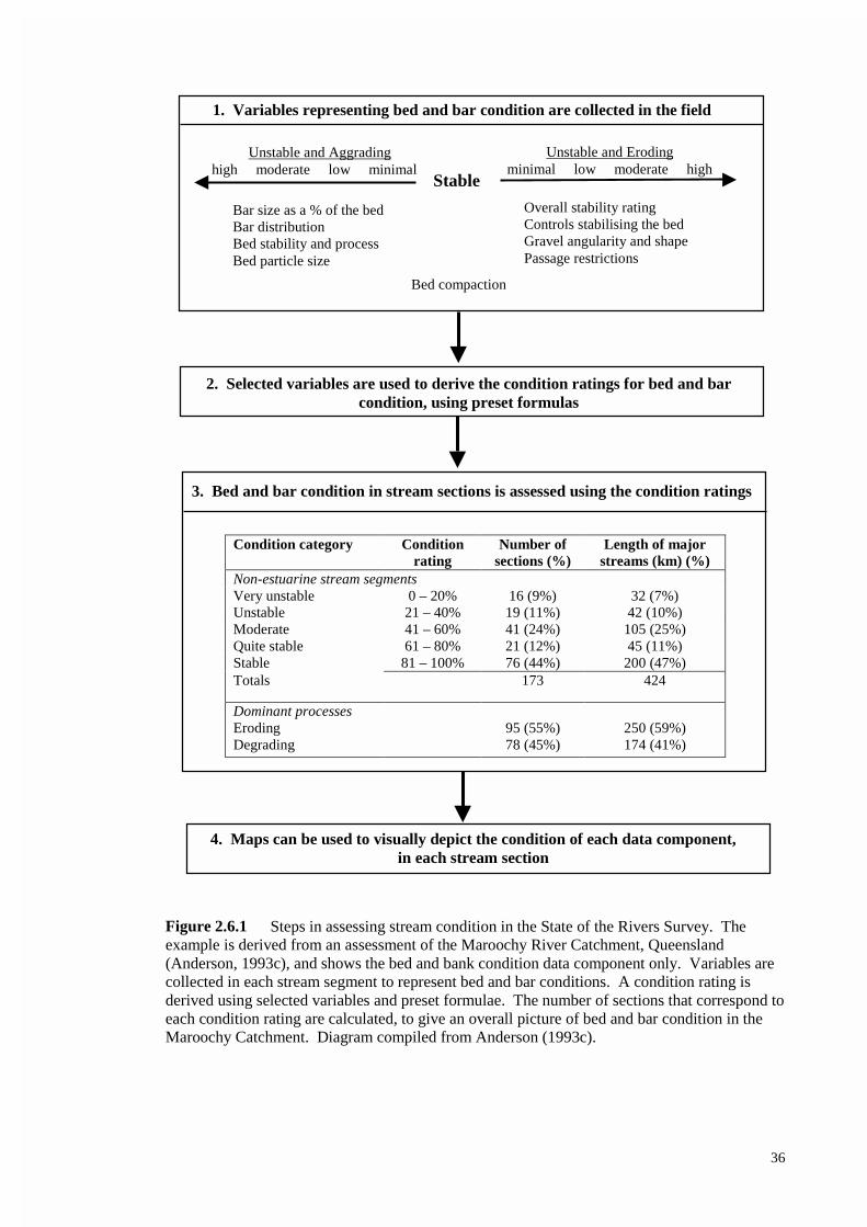
36

Condition category Conditionrating

Number ofsections (%)

Length of majorstreams (km) (%)

Non-estuarine stream segmentsVery unstable 0 – 20% 16 (9%) 32 (7%)Unstable 21 – 40% 19 (11%) 42 (10%)Moderate 41 – 60% 41 (24%) 105 (25%)Quite stable 61 – 80% 21 (12%) 45 (11%)Stable 81 – 100% 76 (44%) 200 (47%)Totals 173 424

Dominant processesEroding 95 (55%) 250 (59%)Degrading 78 (45%) 174 (41%)

Figure 2.6.1 Steps in assessing stream condition in the State of the Rivers Survey. Theexample is derived from an assessment of the Maroochy River Catchment, Queensland(Anderson, 1993c), and shows the bed and bank condition data component only. Variables arecollected in each stream segment to represent bed and bar conditions. A condition rating isderived using selected variables and preset formulae. The number of sections that correspond toeach condition rating are calculated, to give an overall picture of bed and bar condition in theMaroochy Catchment. Diagram compiled from Anderson (1993c).

2. Selected variables are used to derive the condition ratings for bed and barcondition, using preset formulas

Stable

Unstable and Aggradinghigh moderate low minimal

Unstable and Erodingminimal low moderate high

Bar size as a % of the bedBar distributionBed stability and processBed particle size

Overall stability ratingControls stabilising the bedGravel angularity and shapePassage restrictions

Bed compaction

1. Variables representing bed and bar condition are collected in the field

3. Bed and bar condition in stream sections is assessed using the condition ratings

4. Maps can be used to visually depict the condition of each data component,in each stream section

37

primarily makes a detailed assessment of components that describe the physical

condition of streams, such as channel habitat, bed condition, bank condition, cross-

sectional dimension and riparian vegetation (Table 2.6.1). Anderson (1993a)

recognised that habitat attributes of general importance to the biota were encompassed

by these components. Many of the variables measured in the State of the Rivers Survey

correspond with those measured in AUSRIVAS (see Section 2.2), RHS (see Section

2.8) and Habitat Predictive Modelling (see Section 2.7). Therefore, many of the

empirical links between biota and habitat that are encompassed within other methods,

are potentially represented by the variables collected in the State of the Rivers Survey.

2.7 Habitat Predictive Modelling

2.7.1 How did Habitat Predictive Modelling come about?

Habitat Predictive Modelling is a new, novel method that adds a predictive capacity to

assessment of the physical condition of rivers (Davies et al., 2000). As with

AUSRIVAS (see Section 2.2), the major advantage of Habitat Predictive Modelling is

that the features expected to occur at a site can be predicted, thus forming a target

condition against which to measure habitat impairment. This target condition also has

the potential to form the desired state for stream rehabilitation efforts (Davies, 1999).

Additionally, in the absence of water quality degradation, physical habitat will have a

major influence over biotic assemblages (Davies et al., 2000). As such, Habitat

Predictive Modelling complements the AUSRIVAS biological assessments of stream

condition by providing information on whether biotic impairment at a site is related to

poor habitat quality, or to water quality degradation (Davies et al., 2000).

2.7.2 How does Habitat Predictive Modelling work?

Habitat Predictive Modelling uses a similar approach to AUSRIVAS (see Section 2.2),

but uses large-scale catchment features to predict local-scale stream physical habitat

features (Davies et al., 2000). Local-scale habitat features are measured at reference

sites, which are again defined as sites representing least impaired condition (Figure

2.7.1). Classification analysis is then used to form reference sites into groups

containing similar habitat features. Large-scale catchment characteristics, usually

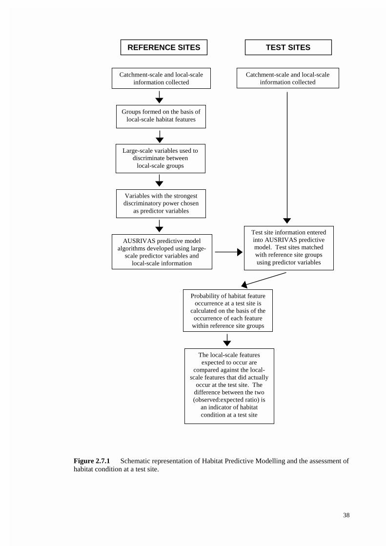
38

Figure 2.7.1 Schematic representation of Habitat Predictive Modelling and the assessment ofhabitat condition at a test site.

Catchment-scale and local-scaleinformation collected

Groups formed on the basis oflocal-scale habitat features

Large-scale variables used todiscriminate between

local-scale groups

Variables with the strongestdiscriminatory power chosen

as predictor variables

Catchment-scale and local-scaleinformation collected

Test site information enteredinto AUSRIVAS predictivemodel. Test sites matchedwith reference site groupsusing predictor variables

AUSRIVAS predictive modelalgorithms developed using large-

scale predictor variables andlocal-scale information

Probability of habitat featureoccurrence at a test site is

calculated on the basis of theoccurrence of each feature

within reference site groups

The local-scale featuresexpected to occur are

compared against the local-scale features that did actually

occur at the test site. Thedifference between the two(observed:expected ratio) is

an indicator of habitatcondition at a test site

REFERENCE SITES TEST SITES

39

measured off maps, are then used to discriminate among the local-scale groups and the

variables with the strongest discriminatory power are chosen as predictor variables for

use in the predictive model algorithm (Figure 2.7.1).

As with AUSRIVAS, the reference site information forms the templet against which test

sites are compared to assess habitat condition (Figure 2.7.1). Local-scale habitat

features are measured at the test sites, along with a suite of larger scale catchment

characteristics that includes the predictor variables. These predictor variables are used

to place test sites into the reference site groups that were formed on the basis of local-

scale habitat features. The model then calculates the probability of occurrence of each

habitat feature at a test site, based on the occurrence of that feature within the

corresponding reference site groups. The habitat features predicted to occur at a test site

are compared against the habitat features that were actually observed at the test site,

with the difference between the two being an indication of habitat condition.

2.7.3 How does Habitat Predictive Modelling assess stream condition?

Habitat Predictive Modelling is based on the observation that stream systems are

organised hierarchically (de Boer, 1992) and that there is a top down control on the

expression of habitat features. For example, Frissell et al. (1986) identified five levels

of hierarchical organisation: stream systems, segment systems, reach systems,

pool/riffle systems and microhabitat subsystems. The characteristics of each level are

constrained by physical processes operating at the next highest level. For example,

climate and geology act at the larger stream system scale to constrain the expression of

bedrock type, longitudinal profile and slope, which are characteristic of the segment

scale. In turn, bedrock, longitudinal profile and slope constrain the development of

reach systems (Frissell et al., 1986). Although Habitat Predictive Modelling does not

aim to capture the same hierarchical levels as Frissell et al. (1986), the prediction of

local-scale habitat features from catchment characteristics reflects the constraining

relationships between physical processes operating at the large and small levels of the

hierarchy. The catchment scale and local-scale variables used in the Habitat Predictive

Modelling approach are listed in Table 2.7.1.

Habitat Predictive Modelling assesses stream condition by comparing the local-scale

habitat features predicted to occur at a site in the absence of degradation, against the

40

Table 2.7.1 List of catchment scale and local scale variables used in Habitat PredictiveModelling. Large-scale variables are the predictor variables and local-scale variables are thehabitat features predicted. After Davies (1999).

Large scale habitat variables Local scale habitat variablesDominant geology in catchment Riparian widthPercent alluvium in catchment Percent trees greater than 10m in heightPercent volcanics in catchment Percent trees less than 10m in heightPercent metasediments in catchment Percent shrubs and vinesPercent limestone in catchment Percent grasses, ferns and sedgesDominant soil type in catchment Shading of reachAnnual mean rainfall Stream widthAnnual median rainfall Bank widthCatchment area Bank heightMaximum catchment length Percent riffle habitatMean catchment slope Riffle depthDifference in elevation between source and mouth Riffle velocityRelief ratio Percent edge habitatDrainage density Edge depthForm ratio Percent boulder in the reachElongation ratio Percent cobble in the reachTotal stream length Percent pebble in the reachValley floor width Percent gravel in the reachValley slope Percent sand in the reachStream order Percent silt in the reachAltitude Percent clay in the reachDistance from source Percent bedrock in the riffleLatitude Percent boulder in the riffleLongitude Percent cobble in the riffleAlkalinity Percent pebble in the riffleConductivity Percent gravel in the rifflepH Percent sand in the riffle

Edge bank vegetationPercent bedrock in the edgePercent boulder in the edgePercent cobble in the edgePercent pebble in the edgePercent gravel in the edgePercent sand in the edgePercent silt in the edgeBottom substrate availability habitatassessment scoreVelocity / depth category habitat assessment scoreChannel alteration habitat assessment scoreScouring habitat assessment scorePool / riffle / run / bend habitat assessment scoreBank stability habitat assessment scoreVegetative stability habitat assessment scoreVegetation cover habitat assessment scoreTotal habitat assessment score

features that were actually observed at a site. The deviation between the two measures

(observed:expected ratio) is an indication of habitat quality. This is the same process

that is used in AUSRIVAS to detect biological impairment (see Section 2.2). However,

in adapting a technique designed to detect biological impairment into a method for

assessing habitat condition, several limitations have become apparent. Firstly,

41

AUSRIVAS predicts the occurrence of macroinvertebrate taxon at a site, whereas, there

is a need with habitat assessment to predict a more continuous type of data. Currently,

the habitat predictive model addresses this by converting each local-scale habitat

variable into categories, prior to classification. However, the use of categorical data can

result in more than one category being predicted to occur at a site, which may result in a

distorted observed:expected ratio (Davies et al., 2000). Secondly, the

observed:expected ratio may provide a resolution that is too coarse to accurately reflect

habitat condition. For example, one site assessed by Davies et al. (2000) demonstrated

an observed:expected ratio of 0.57, which is indicative of impairment. However,

examination of the raw data showed that the site actually contained more trees and

shrubs than predicted, which indicates that riparian vegetation is not a contributing

factor in the habitat impairment observed at this site. Thus, it is suggested that the

habitat features predicted to occur should be checked against the observed habitat

features to determine if the deviation between them actually represents damage to the

stream habitat (Davies et al., 2000). Despite some analytical limitations of Habitat

Predictive Modelling, the technique was successful in predicting small-scale habitat

features, and represents a promising step forward for habitat assessment.

2.7.4 How does Habitat Predictive Modelling link physical and chemical

features with the biota?

Habitat Predictive Modelling is a habitat based approach and thus, it does not attempt to

integrate biological aspects. However, the method has the potential to link physical

features with biota, particularly macroinvertebrates, in two ways:

• Habitat Predictive Modelling can predict the occurrence of local-scale habitat

features that are important to biota, such as riparian vegetation and substratum.

Where specific macroinvertebrate-habitat relationships are known, the absence

of habitat features from a site provides information about the ability of the

habitat to support biota; and,

• the use of similar methods in AUSRIVAS and Habitat Predictive Modelling

provides potential for establishment of empirical relationships between the

observed:expected ratios of the habitat and the biota. This is particularly

relevant if the same reference sites are used to construct the two different

models.

42

2.8 River Habitat Survey

2.8.1 How did the River Habitat Survey come about?

The River Habitat Survey (RHS) is a river assessment method used in the United

Kingdom. The RHS arose from a need to develop a nationally standardised system to

measure, classify and report on the physical structure of rivers (Raven et al., 1997). In

designing the RHS, consideration was given to seven basic requirements. Thus, the

RHS should:

• produce outputs easily understood and used by river and floodplain managers;

• be a tried-and-tested field method, compatible with existing methods such as

river corridor surveys, for use in environmental and post-project appraisal;

• be based on a representative sample of river habitat features;

• have a computer database capable of deriving statistically valid systems for

classification;

• facilitate the description and comparison of physical structure and habitat quality

at catchment, regional and national scales;

• be accepted by external organisations, notably the conservation agencies; and,

• with European Directives in mind, have applicability throughout the UK and

beyond (Raven et al., 1998b).

Information derived from the RHS is designed to assist river management decisions and

provide an ability to predict the physical features of a stream that would occur under

unmodified conditions (Raven et al., 1997). The RHS was conducted in two phases.

The first phase involved the design and testing of survey methods as well as sampling of

a reference site data base of more than 3000 stream sites across the U.K. (Fox et al.,

1998). The second phase is currently under-way and aims to use the RHS in

management applications such as catchment management plans, environmental impact

assessments, stream rehabilitation plans and wildlife conservation (Raven et al., 1998b).

2.8.2 How does the River Habitat Survey work?

The RHS uses the physical structure of streams to assess the character and quality of

rivers (Table 2.8.1). Statistical theory was used to aid the survey design and the

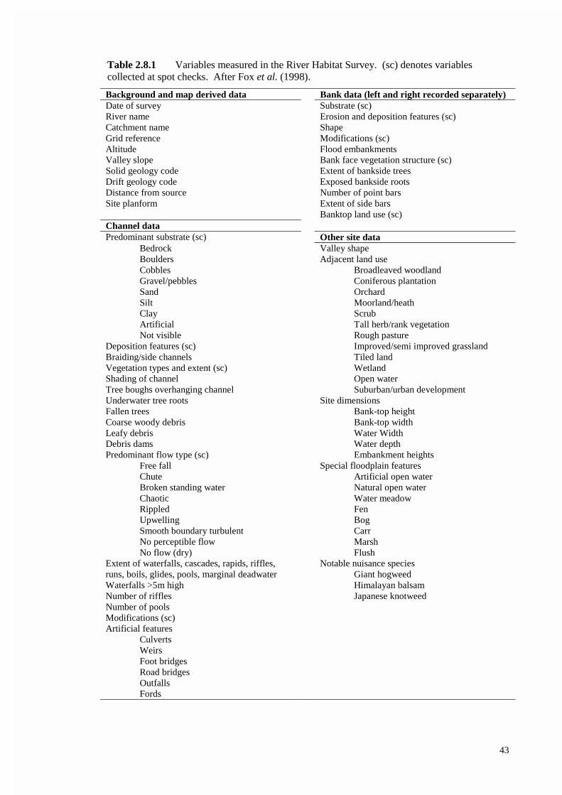
43

Table 2.8.1 Variables measured in the River Habitat Survey. (sc) denotes variablescollected at spot checks. After Fox et al. (1998).

Background and map derived data Bank data (left and right recorded separately)Date of survey Substrate (sc)River name Erosion and deposition features (sc)Catchment name ShapeGrid reference Modifications (sc)Altitude Flood embankmentsValley slope Bank face vegetation structure (sc)Solid geology code Extent of bankside treesDrift geology code Exposed bankside rootsDistance from source Number of point barsSite planform Extent of side bars

Banktop land use (sc)Channel dataPredominant substrate (sc) Other site data

Bedrock Valley shapeBoulders Adjacent land useCobbles Broadleaved woodlandGravel/pebbles Coniferous plantationSand OrchardSilt Moorland/heathClay ScrubArtificial Tall herb/rank vegetationNot visible Rough pasture

Deposition features (sc) Improved/semi improved grasslandBraiding/side channels Tiled landVegetation types and extent (sc) WetlandShading of channel Open waterTree boughs overhanging channel Suburban/urban developmentUnderwater tree roots Site dimensionsFallen trees Bank-top heightCoarse woody debris Bank-top widthLeafy debris Water WidthDebris dams Water depthPredominant flow type (sc) Embankment heights

Free fall Special floodplain featuresChute Artificial open waterBroken standing water Natural open waterChaotic Water meadowRippled FenUpwelling BogSmooth boundary turbulent CarrNo perceptible flow MarshNo flow (dry) Flush

Extent of waterfalls, cascades, rapids, riffles,runs, boils, glides, pools, marginal deadwater

Notable nuisance speciesGiant hogweed

Waterfalls >5m high Himalayan balsamNumber of riffles Japanese knotweedNumber of poolsModifications (sc)Artificial features

CulvertsWeirsFoot bridgesRoad bridgesOutfallsFords

44

selection of sampling sites throughout the U.K. (Jeffers, 1998b, Fox et al., 1998). At

each randomly selected site, a 500m length of river is surveyed. At 50m intervals along

this length of river, 10 spot checks are performed. A range of features is recorded at

each spot check (Table 2.8.1). To ensure that features and modifications not occurring

at the spot checks are included, a sweep up checklist is also completed (Raven et al.,

1998b). In addition, cross sectional measurements of water and bankfull width, bank

height and water depth (Table 2.8.1) are made at one representative location within the

500m sampling site (Raven et al., 1998b). When used in conjunction with the survey

data, these measurements provide information about the geomorphological processes

acting on the site (Raven et al., 1997). Map variables such as altitude, slope, planform

and geology (Table 2.8.1) are measured in the laboratory. Data are entered onto an

electronic database and photos of each sampling site are also stored electronically

(Raven et al., 1998b).

2.8.3 How does the River Habitat Survey assess stream condition?

The RHS takes the view that 'in rivers, habitat is the result of predictable physical

processes and so conveniently sits between the forces which structure rivers and the

biota which inhabit them' (Harper and Everard, 1998 p395). Thus, the RHS measures

variables that represent the character of stream habitats, with the assumption that these

variables reflect the geomorphological processes that are acting to form those habitats

(Newson et al., 1998b). While geomorphological theory underlies many of the

variables collected, the RHS is not strictly a geomorphological survey and specific

measurements of geomorphic processes rates are not considered (Newson et al., 1998b).

In RHS, the basis for assessing habitat quality, using the information collected at

individual 500m sampling sites is:

• quality is based on the presence of channel and river corridor features which are

known to be of value to wildlife;

• the two main factors which determine habitat quality are the diversity and

'naturalness' of physical structure; and,

• the system is calibrated, wherever possible, using known top quality sites

surveyed specifically for this purpose (Raven et al., 1998b).

Habitat quality assessment can be achieved using four main approaches (Figure 2.8.1).

In the first approach, habitat quality is assessed by identifying sites that have pristine

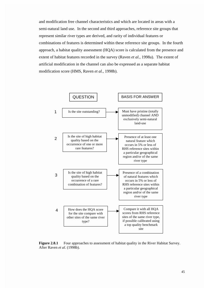
45

and modification free channel characteristics and which are located in areas with a

semi-natural land use. In the second and third approaches, reference site groups that

represent similar river types are derived, and rarity of individual features or

combinations of features is determined within these reference site groups. In the fourth

approach, a habitat quality assessment (HQA) score is calculated from the presence and

extent of habitat features recorded in the survey (Raven et al., 1998a). The extent of

artificial modification in the channel can also be expressed as a separate habitat

modification score (HMS, Raven et al., 1998b).

Figure 2.8.1 Four approaches to assessment of habitat quality in the River Habitat Survey.After Raven et al. (1998b).

Is the site outstanding?

Is the site of high habitatquality based on the

occurrence of one or morerare features?

Is the site of high habitatquality based on theoccurrence of a rare

combination of features?

How does the HQA scorefor the site compare with

other sites of the same rivertype?

QUESTION BASIS FOR ANSWER

Must have pristine (totallyunmodified) channel ANDexclusively semi-natural

land-use

Presence of at least onenatural feature which

occurs in 5% or less ofRHS reference sites withina particular geographicalregion and/or of the same

river type

Presence of a combinationof natural features whichoccurs in 5% or less of

RHS reference sites withina particular geographicalregion and/or of the same

river type

Compare it with all HQAscores from RHS referencesites of the same river type,if possible calibrated using

a top quality benchmarksite

1

2

3

4

46

Although still under investigation, one promising outcome of the RHS is an ability to

predict the features that are likely to occur in a stretch of river, from map based

variables (Jeffers, 1998a). This predictive ability will potentially assist in identifying

the effects of channel modification, as well as enabling targets against which

rehabilitation efforts can be measured.

2.8.4 How does the River Habitat Survey link physical and chemical features

with the biota?

The focus of the RHS on the measurement of habitat quality reflects the underlying

assumption that biotic diversity is directly related to habitat diversity (Harper and

Everard, 1998). To bridge these two concepts, the RHS uses both a biotope and a

functional habitat approach (Newson et al., 1998a). The biotope approach is top down

in that the use of habitat units by biota is inferred from a knowledge physical conditions

(Newson et al., 1998a). The functional habitat approach is bottom up, in that each

habitat is defined from knowledge of the biota that are found in each habitat (Newson et

al., 1998a). Thus, it is assumed that by assessing habitat features within this framework

the physical influences on biotic composition and the physical influences on habitat

formation will both be included.

As mentioned in the previous section, assessment of habitat quality considers the

occurrence of habitat features that are of known value to wildlife. The link between

these features and wildlife is treated slightly differently in each of the four main

approaches. In the first approach, the focus on naturalness reflects the value of this state

to wildlife conservation (Raven et al., 1998a). In the second and third approaches,

rarity can include features that are of known value to wildlife (Raven et al., 1998a). In

the fourth approach, the HQA score considers the presence or absence of features that

are of known wildlife interest (Raven et al., 1998a). While there is an empirical basis

for the relationships between physical features and biotic structure and process (Resh

and Rosenberg, 1984; Harper and Everard, 1998), there is an implicit assumption that

the features included in assessments of habitat quality, and in the RHS in general,

reflect those relationships. This has not been specifically tested, however, one

promising development that may strengthen knowledge in this area is the proposal to

link the RHS with the biological assessment program RIVPACS (Wright et al., 1998).

47

3 SUMMARY AND EVALUATION OF RIVER ASSESSMENT METHODS

3.1 Summary of river assessment methods

The following provides a summary of the advantages and disadvantages of each of the

seven river assessment methods examined in detail in the previous section. Each

method was developed for a different purpose and thus, the use of the term ‘advantages’

and ‘disadvantages’ are not judgements about the relative value of each method as an

individual tool for river assessment. Rather, examination of advantages and

disadvantages is framed in light of the potential for each method, or components of each

method, to fit the requirements of a standardised physical and chemical assessment

protocol, within an AUSRIVAS style framework.

3.1.1 AUSRIVAS

Advantages

• Nationally standardised biomonitoring approach

• Uses biota as the endpoint to represent environmental condition

• Comparisons to reference condition establish level of biological impairment

• Capability to predict taxon occurrence at sites

• Incorporates established empirical links between the biota and some of the

physical and chemical variables used as predictor variables (e.g. substratum,

riparian vegetation, altitude)

• Outputs easily understood by managers, scientists and community groups

Potential disadvantages

• Limited ability to link causal factors (water quality degradation, habitat

quality degradation or both) to biological condition

• Assumes that all the major physical, chemical and habitat factors with an

empirical link to macroinvertebrate community structure and which can

provide an independent way of matching test sites with reference site groups,

were included in constructing the predictive models

• Limited ability to predict macroinvertebrate community structure in large

river systems

Sampling and data collection issues

• Requires collection of an extensive reference site database to develop models

48

• Rapid sampling philosophy - approximately 1 hour field work and 1-3 hours

laboratory work per site

• Small deviations in methods can limit model capabilities (e.g. live pick and

laboratory sort data are not interchangeable)

3.1.2 HABSCORE

Advantages

• Integrates habitat parameters into a score that represents a continuum of

conditions for biota. Reference conditions are considered optimal.

• Can be used without modification in other monitoring programs (e.g.

AUSRIVAS)

• Habitat parameters are used to determine the ability of the habitat to support

biota

• Habitat parameters represent aspects of the habitat that are related to aquatic

life use

• Additional site observations aid interpretation of biological condition at a

site

Potential disadvantages

• Most criticism is of the multimetric approach to biomonitoring, rather than

of the HABSCORE method

• Subject to operator differences in interpretation and scoring of the habitat

parameters (Hannaford and Resh, 1995)

Sampling and data collection issues

• Rapid sampling philosophy – approximately 15min per site to assess habitat

parameters

3.1.3 Index of Stream Condition

Advantages

• Used for long term assessments of whole stream reaches

• Integrates several key components of stream condition (hydrology, physical

form, streamside zone, water quality and aquatic life)

• Management orientated, with a scientific basis. Also useful as a tool for

monitoring management interventions

49

• Indices can be weighted according to their perceived importance, or

according to data availability

• The reference state ratings are based on knowledge of levels of stress that

cause biological community degradation (e.g. pH, riparian vegetation cover)

Potential disadvantages

• Designed to be repeated every five years, so it has limited suitability for

routine monitoring programs

• Reach scale and long term assessment focus means that it may not be

detailed or sensitive enough to pick up all perturbations

• Information on the link between a change in index value and a

corresponding change in environmental condition is limited

• Determination of reference condition is subjective

Sampling and data collection issues

• Field assessment takes approximately 2 hours at a site. Desk based data

collection is also required

3.1.4 Geomorphic River Styles

Advantages

• Foundation in geomorphological theory

• Measures habitats, or physical structure at different scales

• Ability to predict future river character and responses to disturbance, based

on geomorphological process theory

• Habitat based links between geomorphology and biota

• Set within a hierarchical framework

Potential disadvantages

• Assumes that the habitat units considered are relevant to biota

• Requires a high level of geomorphological expertise, particularly for

interpretation and prediction

• Establishment of the benchmark reference condition is subjective and

requires a high level of geomorphological expertise to determine

• Indirect, rather than direct links to river ecology

• Limited testing of the links between geomorphological parameters and biota.

For example, is the distribution of geomorphological process zones related to

the distribution of the biota?

50

Sampling and data collection issues

• Air-photos may not be available for some areas, to delineate stream reaches

• Specialised equipment may be required for surveying

3.1.5 State of the Rivers Survey

Advantages

• Comprehensive coverage of stream sections within a catchment

• Assessment of at many levels - whole catchment, individual sections or

individual tributaries, using data components individually or together

• Use of homogeneous stream sections allows extrapolation from the sampling

scale to larger areas

• Physical measurements indirectly represent geomorphological processes

• Some empirical links between the parameters measured and stream biota

(e.g. substratum, riparian vegetation)

Potential disadvantages

• Comparisons to reference condition are subjective

• Links between some measured parameters (e.g. bank condition, bar shape)

and biota are not well established

• Links between structure and process are weak

Sampling and data collection issues

• Rapid sampling philosophy - 3/4 to 1 hour per site in the field

• Some desk based data collection also required

3.1.6 Habitat Predictive Modelling

Advantages

• Ability to predict the occurrence of stream habitat features

• Ability to incorporate variables that are directly relevant to biota, as well as

variables that are based on geomorphological processes

• Comparisons to reference condition establish habitat impairment

• Use of a method identical to AUSRIVAS may facilitate direct comparison of

macroinvertebrate and habitat observed:expected scores

• Set within a hierarchical framework

51

Potential disadvantages

• Choice of variables may affect predictive ability. Emphasis on biological

variables may facilitate links to AUSRIVAS outputs, however,

geomorphological process variables may also be important for predicting

habitat features

• Currently subject to some analytical limitations (e.g. prediction of categories

rather than continuous data)

Sampling and data collection issues

• Can make use of data collected for the existing AUSRIVAS program

• Depending on the choice of variables, rapid sampling philosophies can

potentially be applied to data collection

3.1.7 River Habitat Survey

Advantages

• Geomorphological theory underlies many of the variables collected

• Uses the functional habitat and biotope philosophies to link physical habitat

with the biota

• Several mechanisms available to determine habitat quality and identify

benchmark sites

• Nationally standardised approach

• Potential for linkage with the RIVPACS biological assessment program

Disadvantages

• Links between biota some of the habitat components measured are not well

established

• Counts of classes the only feasible data form for most measurements. Thus,

the mixture of qualitative and quantitative data, with nominal, ordinal and

interval types makes statistical tests difficult

Sampling and data collection issues

• Requires collection of an extensive database to determine initial stream types

• Problems were identified with operator differences - this necessitated the use

of occurrence rather than quantitative data, which subsequently reduced the

ability for statistical analysis

• Rapid sampling philosophy - approximately 1 hour per site in the field

52

3.2 Evaluation of river assessment methods

Each of the river assessment methods considered in this review was developed for a

specific purpose and thus, the methods reflect a range of management goals and

scientific approaches. However, development of a standardised protocol for the

physical and chemical assessment of river condition requires consideration of the

following specific qualities:

• scale of focus that is commensurate with the AUSRIVAS biological

monitoring protocol;

• capacity to measure stream condition against a desirable reference state;

• incorporation of parameters that are relevant to the biota, especially

macroinvertebrates;

• representation of important geomorphological processes that influence the

formation of stream habitat;

• conformity with a rapid philosophy of data collection and analysis;

• potential for use by non-experts;

• scientific outputs presented in a form that is easily interpreted by managers;

• adaptability and applicability to a wide range of river types across Australia;

and,

• ability to predict physical stream characteristics.

The representation of each of these qualities within the seven river assessment methods

examined in this review is summarised in Table 3.2.1. Overall, the methods generally

use rapid data collection and analysis methods, they have the potential for use by non-

experts and their scientific outputs are presented in a form that is easily interpreted by

managers (Table 3.2.1). Each of the methods also has some capacity to assess stream

condition against a reference state, however, the degree to which this function is utilised

in determining site condition varies among the methods. Similarly, the methods vary

widely in predictive ability, applicability to a wide range of river types across Australia

and scale of focus (Table 3.2.1). Differences between the dominant paradigms of

stream ecology and geomorphology are reflected by two criteria: the incorporation of

parameters relevant to biota and the representation of important geomorphological

processes (Table 3.2.1). Geomorphic River Styles, State of the Rivers Survey and River

Habitat Survey were each designed to assess physical or geomorphological aspects of

streams and thus, they attempt to incorporate empirical relationships between physical

parameters and biota indirectly. Conversely, AUSRIVAS, HABSCORE and Index of

Stream Condition have a strong biological component and thus, they fail to fully

53

Table 3.2.1 Evaluation of seven river assessment methods against the desired qualities of a standardised physical and chemical assessment protocol. Therepresentation of each of the qualities by the methods is designated as yes (Y), no (N), potentially (P) or indirectly (I).

Desired qualities of the physical and chemical Potential methods for inclusion in the physical and chemical assessment protocolassessment protocol

AUSRIVAS HABSCOREIndex ofStream

Condition

GeomorphicRiver Styles

State of theRiversSurvey

HabitatPredictiveModelling

River HabitatSurvey

Scale of focus commensurate with the AUSRIVASbiological monitoring protocol Y Y N P P Y PCapacity to measure stream condition against adesirable reference state Y Y Y I Y Y IIncorporation of parameters that are relevant to thebiota, particularly macroinvertebrates Y Y Y P P Y PRepresentation of important geomorphologicalprocesses that influence the formation of stream habitat N N N Y I P YConformity with a rapid philosophy of data collectionand analysis Y Y N N Y Y YPotential for use by non-experts

Y Y Y N Y Y YScientific outputs presented in a form that is easilyinterpreted by managers Y Y Y P Y Y YAdaptability and applicability to a wide range of rivertypes across Australia Y P P P P Y PAbility to predict physical stream characteristics

Y N N Y N Y P

54

consider geomorphological processes. Finding common ground between biologically

and geomorphologically relevant parameters would provide a more holistic perspective

on the assessment of stream condition.

3.3 Future directions - habitat assessment workshop

As discussed in Section 1.1, development of a protocol for the physical assessment of

stream condition that is complementary to AUSRIVAS requires simultaneous

consideration of biological and geomorphological methods and approaches. This

review is a first step towards merging the two approaches to stream assessment, and

provides an information base that that will be built upon at the habitat assessment

workshop, scheduled for 2-3 May, 2000. The habitat assessment workshop will bring

together geomorphologists, hydrologists and ecologists and will involve the authors of

several of the methods covered in this review. The aim of the workshop is to develop a

framework for a standardised physical and chemical assessment protocol. One of the

main challenges of the workshop will be to determine the physical variables that are

relevant to biota, and to determine the most suitable methods for measuring these

variables in a cost effective manner, and within a rapid sampling philosophy.

Specifically, it is hoped that the questions posed in Section 1.1 will be answered in

detail during the course of the workshop to form the basis for a standardised physical

and chemical assessment protocol. The outcomes and recommendations from the

habitat assessment workshop will be reported in a future document.

55

4 REFERENCES

Anderson, J.R. (1993a) State of the Rivers Project. Report 1. Development andValidation of the Methodology. Department of Primary Industries, Queensland.

Anderson, J.R. (1993b) State of the Rivers Project. Report 2. ImplementationManual. Department of Primary Industries, Queensland.

Anderson, J.R. (1993c) State of the Rivers: Maroochy River and Tributary Streams.Report to Maroochy Shire Council and Queensland Department of PrimaryIndustries.

Anderson, J.R. (1999) Basic Decision Support System for Management of UrbanStreams. Report A: Development of the Classification System for UrbanStreams. National River Health Program, Urban Sub Program. LWRRDCOccasional Paper 8/99.

Barbour, M.T. (1991) Stream surveys - the importance of the relation between habitatquality and biological condition. Sediment and Stream Water Quality in aChanging Environment: Trends and Explanation. Proceedings of the ViennaSymposium, August 1991. IAIIS Publication No. 203.

Barbour, M.T., Gerritsen, J., Snyder, B.D. and Stribling, J.B. (1999) Rapidbioassessment protocols for use in streams and wadeable rivers: periphyton,benthic macroinvertebrates and fish. Second edition. EPA 841-B-99-002. U.S.Environmental Protection Agency, Office of Water, Washington.

Boon, P.J., Wilkinson, J. and Martin, J. (1998) The application of SERCON (Systemfor Evaluating Rivers for Conservation) to a selection of rivers in Britain.Aquatic Conservation: Marine and Freshwater Ecosystems, 8: 597-616.

Brierley, G., Fryirs, K. and Cohen, T. (1996) Development of a generic geomorphicframework to assess catchment character. Part 1. A geomorphic approach tocatchment characterisation. Working Paper 9603, Macquarie University,Graduate School of the Environment.

Brierley, G.J., Cohen, T., Fryirs, K. and Brooks, A. (1999) Post-European changes tothe fluvial geomorphology of Bega catchment, Australia: implications for riverecology. Freshwater Biology, 41: 839-848.

Chessman, B. and Nancarrow, J. (1999) Draft pressure-biota-habitat streamassessment. Report on Adelong Creek field trial. New South Wales Departmentof Land and Water Conservation, Sydney.

Cohen, T., Brierley, G. and Fryirs, K. (1996) Development of a generic geomorphicframework to assess catchment character. Part 2. Fluvial geomorphology andriver ecology of coastal rivers in southeastern Australia. Working Paper 9603,Macquarie University, Graduate School of the Environment.

Cooper, S.D., Diehl, S., Kratz, K. and Sarnelle, O. (1998) Implications of scale forpatterns and processes in stream ecology. Australian Journal of Ecology, 23:27-40.

56

Coysh, J., Nichols, S., Simpson, J., Norris, R., Barmuta, L., Chessman, B. andBlackman, P. (2000) AUSRIVAS predictive model manual. CooperativeResearch Centre for Freshwater Ecology, Canberra.http://enterprise.canberra.edu.au/Databases/AusRivAS.nsf/

Davies, N.M. (1999) Prediction and assessment of local stream habitat features usinglarge-scale catchment characteristics. Unpublished Honours Thesis, Universityof Canberra. 96pp.

Davies, N.M., Norris, R.H. and Thoms, M.C. (2000) Prediction and assessment oflocal stream habitat features using large-scale catchment characteristics.Freshwater Biology, 45: 343-369.

de Boer, D.H. (1992) Hierarchies and spatial scale in process geomorphology: areview. Geomorphology, 4: 303-318.

DNRE (1997) An Index of Stream Condition: Users Manual. Department of NaturalResources and Environment, Government of Victoria, Melbourne.

Fox, P.J.A., Naura, M. and Scarlett, P. (1998) An account of the derivation and testingof a standard field method, River Habitat Survey. Aquatic Conservation:Marine and Freshwater Ecosystems, 8: 455-475.

Frissell, C.A., Liss, W.J., Warren, C.E. and Hurley, M.D. (1986) A hierarchicalframework for stream habitat classification: viewing streams in a watershedcontext. Environmental Management, 10: 199-214.

Fryirs, K., Brierley, G. and Cohen, T. (1996) Development of a generic geomorphicframework to assess catchment character. Part 3. Application of the catchmentcharacterisation procedure to Wolumla Creek Catchment, South Coast, NewSouth Wales. Working Paper 9603, Macquarie University, Graduate School ofthe Environment.

Hannaford, M.J. and Resh, V.H. (1995) Variability in macroinvertebrate rapid-bioassessment surveys and habitat assessment in a northern California stream.Journal of the North American Benthological Society, 14: 430-439.

Harper, D., Smith, C., Barham, P. and Howell, R. (1995) The ecological basis of themanagement of the natural river environment. In: Harper, D.M. and Ferguson,A.J.D. (eds.) The Ecological Basis for River Management. John Wiley andSons, Chichester. pp. 219-238.

Harper, D. and Everard, M. (1998) Why should the habitat-level approach underpinholistic river survey management? Aquatic Conservation: Marine andFreshwater Ecosystems, 8: 395-413.

Jeffers, J.N.R. (1998a) Characterization of river habitats and prediction of habitatfeatures using ordination techniques. Aquatic Conservation: Marine andFreshwater Ecosystems, 8: 529-540.

57

Jeffers, J.N.R. (1998b) The statistical basis of sampling strategies for rivers: anexample using River Habitat Survey. Aquatic Conservation: Marine andFreshwater Ecosystems, 8: 447-454.

Ladson, A.R. and White, L.J. (1999) An Index of Stream Condition: ReferenceManual. Department of Natural Resources and Environment, Melbourne, April1999.

Ladson, A.R., White, L.J., Doolan, J.A., Finlayson, B.L., Hart, B.T., Lake, P.S. andTilleard, J.W. (1999) Development and testing of an Index of Stream Conditionfor waterway management in Australia. Freshwater Biology, 41: 453-468.

Ladson, A.R. and White, L.J. (2000) Measuring stream condition. In: Brizga, S. andFinlayson, B. (eds.) River Management, The Australasian Experience. JohnWiley and Sons, Chichester. pp. 265-285.

Maddock, I. (1999) The importance of physical habitat assessment for evaluating riverhealth. Freshwater Biology, 41: 373-391.

McMillan, P.H. (1998) An integrated habitat assessment system (IHAS v2) for therapid biological assessment of rivers and streams. Research Project numberENV-P-I-98132. Council for Scientific and Industrial Research (CSIR), WaterResources Management Programme, South Africa.

Montgomery, D.R. (1999) Process domains and the river continuum. Journal of theAmerican Water Resources Association, 35: 397-410.

Moss, D., Furse, M.T., Wright, J.F. and Armitage, P.D. (1987) The prediction of themacro-invertebrate fauna of unpolluted running-water sites in Great Britainusing environmental data. Freshwater Biology, 17: 41-52.

Muhar, S. and Jungwirth, M. (1998) Habitat integrity of running waters – assessmentcriteria and their biological relevance. Hydrobiologia, 386: 195-202.

Newson, M.D., Clark, M.J., Sear, D.A. and Brookes, A. (1998b) Thegeomorphological basis for classifying rivers. Aquatic Conservation: Marineand Freshwater Ecosystems, 8: 415-430.

Newson, M.D., Harper, D.M., Padmore, C.L., Kemp, J.L. and Vogel, B. (1998a) Acost-effective approach for linking habitats, flow types and speciesrequirements. Aquatic Conservation: Marine and Freshwater Ecosystems, 8:431-446.

Norris, R.H. and Thoms, M.C. (1999) What is river health? Freshwater Biology, 41:197-209.

O'Connor, N. (1999) Mid-term Review of The Natural Heritage Trust. A review of theNational River Health Program. Environment Australia, Canberra.http://www.nht.gov.au/review/mtrfinrpt/natrivhealth.pdf

58

Plafkin, J.L., Barbour, M.T., Porter, K.D., Gross, S.K. and Hughes, R.M. (1989) Rapidbioassessment protocols for use in streams and rivers: benthicmacroinvertebrates and fish. EPA/444/4-89-001. U.S. EnvironmentalProtection Agency, Office of Water, Washington.

Rankin, E.T. (1995) Habitat indices in water resource quality assessments. In: Davis,W.S. and Simon, T.P. (eds.) Biological Assessment and Criteria: Tools forWater Resource Planning and Decision Making. CRC Press, Boca Raton. pp.181-208.

Raven, P.J., Fox, P., Everard, M., Holmes, N.T.H. and Dawson, F.H. (1997) Riverhabitat survey: a new system for classifying rivers according to their habitatquality. In: Boon, P.J. and Howell, D.L. (eds.) Freshwater Quality: Definingthe Indefinable? The Stationery Office, Edinburgh. pp. 215-234.

Raven, P.J., Holmes, N.T.H., Dawson, F.H. and Everard, M. (1998a) Qualityassessment using River Habitat Survey data. Aquatic Conservation: Marine andFreshwater Ecosystems, 8: 477-499.

Raven, P.J., Holmes, N.T.H., Dawson, F.H., Fox, P.J.A., Everard, M., Fozzard, I.R. andRouen, K.J. (1998b) River Habitat Quality: The Physical Character of Riversand Streams in the UK and Isle of Man. River Habitat Survey, Report No. 2.Environment Agency, Bristol, U.K.

Reice, S.R. and Wohlenberg, M. (1993) Monitoring freshwater benthicmacroinvertebrates and benthic processes: measures for assessment ofecosystem health. In: Rosenberg, D.M. and Resh, V.H. (eds.) FreshwaterBiomonitoring and Benthic Macroinvertebrates. Chapman and Hall, New York.pp. 287-305.

Resh, V.H. and Rosenberg, D.M. (1984) The Ecology of Aquatic Insects. Praeger,New York.

Resh, V.H., Hildrew, A.G., Statzner, B. and Townsend, C.R. (1994) Theoreticalhabitat templets, species traits, and species richness: a synthesis of long-termecological research on the Upper Rhone River in the context of concurrentlydeveloped ecological theory. Freshwater Biology, 31: 539-554.

Reynoldson, T.B., Norris, R.H., Resh, V.H., Day, K.E. and Rosenberg, D.M. (1997)The reference condition: a comparison of multimetric and multivariateapproaches to assess water-quality impairment using benthicmacroinvertebrates. Journal of the North American Benthological Society, 16:833-852.

Rosenberg, D.M. and Resh, V.H. (1993) Introduction to freshwater biomonitoring andbenthic macroinvertebrates. In: Rosenberg, D.M. and Resh, V.H. (eds.)Freshwater Biomonitoring and Benthic Macroinvertebrates. Chapman andHall, New York. pp. 1-9.

Sale, P.F. (1998) Appropriate spatial scales for studies of reef-fish ecology. AustralianJournal of Ecology, 23: 202-208.

59

Schumm, S.A. (1977) The Fluvial System. John Wiley and Sons, New York.

Simpson, J.C. and Norris, R.H. (2000) Biological assessment of river quality:development of AUSRIVAS models and outputs. In: Wright, J.F., Sutcliffe,D.W. and Furse, M.T. (eds.) Assessing the biological quality of freshwaters.RIVPACS and other techniques. Freshwater Biological Association, Ambelside.pp. 125-142.

Townsend, C.R. and Hildrew, A.G. (1994) Species traits in relation to a habitat templetfor river systems. Freshwater Biology, 31: 265-275.

Vinson, M.R. and Hawkins, C.P. (1998) Biodiversity of stream insects: variation atlocal, basin and regional scales. Annual Review of Entomology, 43: 271-293.

Ward, J.V. (1992) Aquatic Insect Ecology: Biology and Habitat. John Wiley andSons, New York.

Weins, J.A. (1989) Spatial scaling in ecology. Functional Ecology, 3: 385-397.

Wright, J.F., Moss, D., Armitage, P.D. and Furse, M.T. (1984) A preliminaryclassification of running-water sites in Great Britain based on macro-invertebrate species and the prediction of community type using environmentaldata. Freshwater Biology, 14: 221-256.

Wright, J.F., Furse, M.T. and Moss, D. (1998) River classification using invertebrates:RIVPACS applications. Aquatic Conservation: Marine and FreshwaterEcosystems, 8: 617-631.