
Australia and the global financial crisis · Australia and the global financial crisis Grete...
96
1 Australia and the global financial crisis Grete Refsahl Advisor: Jan Tore Klovland Master thesis – Department of Finance and Management Science NORGES HANDELSHØYSKOLE This thesis was written as a part of the Master of Science in Economics and Business Administration program - Major in Financial Economics. Neither the institution, nor the advisor is responsible for the theories and methods used, or the results and conclusions drawn, through the approval of this thesis. NORGES HANDELSHØYSKOLE Bergen, 18.06.2010
Transcript of Australia and the global financial crisis · Australia and the global financial crisis Grete...
1
Australia and the global financial crisis
Grete Refsahl
Advisor: Jan Tore Klovland
Master thesis – Department of Finance and Management Science
NORGES HANDELSHØYSKOLE
This thesis was written as a part of the Master of Science in Economics and Business Administration program - Major in Financial Economics. Neither the institution, nor the advisor is responsible for the theories and methods used, or the results and conclusions drawn, through the approval of this thesis.
NORGES HANDELSHØYSKOLEBergen, 18.06.2010

2
3
ABSTRACT
This paper targets the question of why the Australian economy dealt so well with the global financial
crisis in the period July 2007 – February 2010. Part One investigates the question from a descriptive
angle, providing a brief outline of the conditions in various domestic markets. In Part Two,
econometric tools are employed to construct a model of the Australian dollar. The short‐run
dynamics are addressed and the results indicate that while some influential factors have changed the
direction of their impact on the floating Australian dollar, other relationships have remained intact or
even strengthened during the financial crisis. The empirical results imply that part of the explanation
can be ascribed to the exchange rate and how it acts as a shock absorber for the domestic economy.
4
Table of Contents
ABSTRACT ........................................................................................................................................................... 3
PREFACE .............................................................................................................................................................. 7
OUTLINE OF STRUCTURE AND PROBLEM FORMULATION ................................................................. 8
PART ONE ........................................................................................................................................................... 9
CHAPTER 1. INTRODUCTION, PART ONE ............................................................................................... 10
CHAPTER 2. THE RESERVE BANK OF AUSTRALIA ............................................................................... 12
2.1 Monetary policy and the conduction thereof ............................................................................. 12
2.2 Market intervention and other policy measures in recent time ................................................. 13
2.3 Intervention in the foreign exchange market ............................................................................. 15
CHAPTER 3. THE CREDIT MARKET .......................................................................................................... 17
3.1 Banking sector ............................................................................................................................. 17
3.2 Household borrowing .................................................................................................................. 18
3.3 Corporate borrowing ................................................................................................................... 19
3.4 The Bond market ......................................................................................................................... 20
3.5 Residential Mortgage‐Backed Securities (RMBS) ........................................................................ 21
CHAPTER 4. THE EQUITY MARKET .......................................................................................................... 22
CHAPTER 5. DOMESTIC DEMAND ............................................................................................................. 25
5.1 Fiscal policy and stimulus packages ............................................................................................ 26
5.2 Other factors of relevance........................................................................................................... 28
CHAPTER 6. INTERNATIONAL CONDITIONS AND DOMESTIC PRODUCTION ............................. 31
6.1 The global environment .............................................................................................................. 31
6.2 The situation for domestic production during the crisis ............................................................. 32
6.3 The export sector ........................................................................................................................ 33
6.4 Australia’s trading partners ......................................................................................................... 35
6.5 The relationship between Terms of Trade and the exchange rate ............................................. 36
5
6.6 Current climate for domestic production .................................................................................... 37
CHAPTER 7. EXCHANGE RATE DEVELOPMENTS ................................................................................. 38
7.1 The Australian dollar – relative to what? .................................................................................... 38
7.2 Development of the Australian dollar‐ July 2007 to February 2010 ........................................... 39
CHAPTER 8. SUMMARY, PART ONE .......................................................................................................... 42
PART TWO ....................................................................................................................................................... 43
CHAPTER 9. INTRODUCTION, PART TWO .............................................................................................. 44
CHAPTER 10. THE FOREIGN EXCHANGE MARKET .............................................................................. 46
10.1 Some general facts about the foreign exchange market .......................................................... 46
10.2 The Purchasing Power Parity (PPP) hypothesis ......................................................................... 48
10.3 The Uncovered Interest Parity (UIP) relationship ..................................................................... 49
10.4 The Real Interest Parity (RIP) relationship – The Fisher Equation ............................................ 50
10.5 The relationship between the Australian dollar and Terms of Trade. An overview of previous analyses. ............................................................................................................................................ 52
CHAPTER 11. THE MODEL VARIABLES ................................................................................................... 55
11.1 The dependent variable: Nominal exchange rate, “TWI/AUD” ................................................ 55
11.2 The independent variables ........................................................................................................ 56
11.3 Final remarks ............................................................................................................................. 60
CHAPTER 12. TIME SERIES AND THEIR SUITABILITY FOR REGRESSION ANALYSIS ............... 61
12.1 Necessary characteristics .......................................................................................................... 61
12.2 Dickey Fuller test for stationarity .............................................................................................. 61
12.3 Augmented Dickey Fuller test ................................................................................................... 62
12.4 Cointegration ............................................................................................................................. 63
12.5 The spurious regression problem .............................................................................................. 64
12.6 Interpretation of a regression estimate .................................................................................... 65
CHAPTER 13. EMPIRICAL RESULTS ......................................................................................................... 67
13.1 Results from the Augmented Dickey Fuller‐test ....................................................................... 67
6
13.2 Dickey Fuller test for cointegration ........................................................................................... 68
13.3 Implications of the tests ............................................................................................................ 69
13.4 The OLS regression model ......................................................................................................... 71
13.5 Interpretation of the results ...................................................................................................... 74
13.6 Limitations of the model ........................................................................................................... 79
CHAPTER 14. SUMMARY, PART TWO ...................................................................................................... 82
CHAPTER 15. CONCLUSION ........................................................................................................................ 84
REFERENCES ................................................................................................................................................... 85
APPENDIX A. THE VARIANCE INFLATION FACTOR (VIF) ................................................................. 92
APPENDIX B. MINITAB BEST SUBSET PROCEDURE ............................................................................ 93
7
PREFACE
The purpose of this thesis is to investigate how the Australian economy was affected by the global
financial crisis emerging in 2007. For many nations, this transformed into a real economic recession,
creating a heavy burden for their governments and citizens. The author of this thesis lived in Sydney
the first half of 2009, and the general impression was that there didn’t seem to be a recession in the
economy at all. This spurred an interest in how such an outcome is possible for a relatively young
nation (the Commonwealth of Australia was established in 1901). In May 1986, the Australian
Government Treasurer Paul Keating compared the nation’s economic development to a “banana
republic” due to its large Current Account deficit. In the following weeks, the Australian dollar
depreciated by more than 10 per cent. 24 years ago, those two words pushed the Australian financial
markets out of balance. How the same nation today can battle a global financial crisis and avoid
recession altogether is therefore a very relevant question.
Before embarking on the task of describing and analyzing the development with a framework of
economic theory, some first‐hand observations might be of interest. My impression is that the
Australian public seemed quite relaxed about the global financial situation. Newspapers and
television programmes did not have an excessive focus on disasters in financial markets or gloomy
economic outlook, the way media in other developed countries have had. No doubt was this partly
because it was not necessary, the Australian economy held up well. But it also demonstrates how the
creation of irrational fear in the public does not benefit the economy as a whole. Consumer
confidence and domestic demand is very influential forces when it comes to dealing with a recession.
Therefore, the rational attitude of the Australian media might have played a part in getting the
nation back on its feet so early. This however, is a theory impossible to prove. Therefore, my focus
will be on which factors contributed to absorbing or counteracting the external shock the Australian
economy was exposed to.
I’d like to thank my thesis advisor, Professor Jan Tore Klovland. Without his pragmatic approach to
my questions and concerns, I would surely never have completed this task. A thank you is also due to
fellow students, who have helped me navigate through the jungle of databases available. Finally, my
gratitude towards friends and family must be expressed. Without them, this thesis would have
merely been a fleeting idea.
8
OUTLINE OF STRUCTURE AND PROBLEM FORMULATION
Due to practical considerations, this thesis is structured as comprising of two parts: The first part will
provide an overview of the Australian economy and its development during the period July 2007 –
February 2010. This part will be of a descriptive nature, aimed to give a brief outline of the
macroeconomic situation in Australia and prepare the reader for Part Two. Part Two will examine the
question of how and why the Australian exchange rate has behaved as witnessed during this
financially turbulent period of time. Here, an empirical model of the Australian dollar will be
presented and analyzed. Although the independent findings of this thesis are located in Part Two, it is
strongly recommended to read Part One first, as this is important and necessary background
information in order for the reader to fully understand the results of the empirical analysis.
The two parts of this thesis differ with respect to the set of tools employed. However, they are
strongly linked by a common underlying purpose. They both intend to answer the following problem
formulation:
Why did the Australian economy cope so well with the 2007/2008 global financial crisis?
The problem formulation is far‐reaching, and a bit vague. That is intentional. Too many specifications
may cause important information to be excluded before the overall picture is well‐understood. In
order for other countries to learn from the Australian experience, one must consider the question
from several different angles – the descriptive, the empirical and the intuitive.

9
PART ONE
THE DESCRIPTIVE APPROACH
10
CHAPTER 1. INTRODUCTION, PART ONE
Part One of the thesis is the result of a literary study. It provides a descriptive overview of the
Australian economy in the period July 2007 to February 2010. The aim is to identify and describe
characteristics of the Australian economy which have contributed to the resilience and recovery of
the nation’s economic health.
Part One is structured as follows: Starting by describing the central bank, its role, and instruments of
monetary policy, I then move on to the domestic financial markets and explain how they have been
affected by the crisis. Next, development in domestic demand and production will be treated and
Government fiscal policy measures are discussed. By treating each market in isolation, moving from
one to the next I finally arrive at the one channel linking all the prior sections of the economy: The
exchange rate.
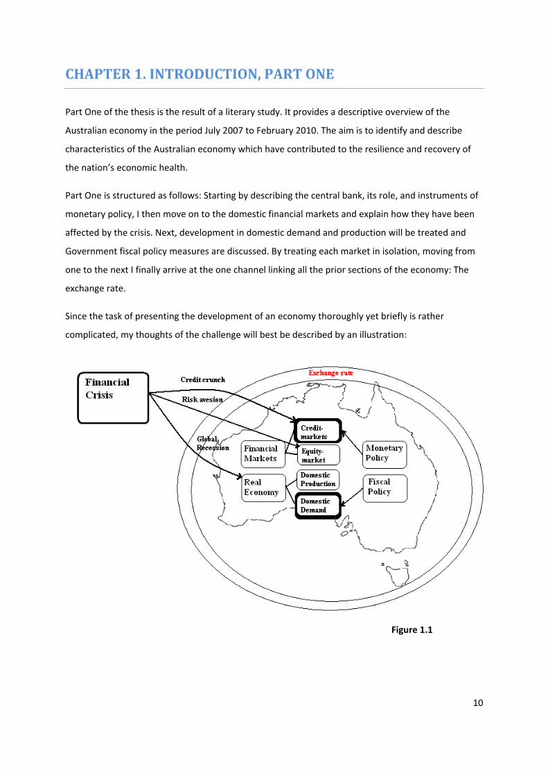
Since the task of presenting the development of an economy thoroughly yet briefly is rather
complicated, my thoughts of the challenge will best be described by an illustration:
Figure 1.1
11
The arrows from the box “Financial crisis” represent the external shock to the Australian economy
and which channels it feeds through to different sections of the economy. The thick outlines are the
“shields”, provided by the Government and the Central Bank. The double line around the country
represents how the floating exchange rate acts as a natural absorber to external shocks. The
illustration is not extensive with respect to the dynamics of the relationships, or how Government
policies have counteracted the crisis. However, it does provide an adequate presentation of how Part
One is structured.
The dominant source of information for Part One is the webpage of the Australian Central Bank1.
Here, the abundance of statements, reports and forecasts available provides detailed treatment of
the markets addressed. However, referring to each publication in the text separately would severely
compromise its presentational quality with respect to the reader. Therefore, unless otherwise stated,
the Reserve Bank of Australia is the source of facts presented in Part One.
1 www.rba.gov.au
12
CHAPTER 2. THE RESERVE BANK OF AUSTRALIA
2.1 Monetary policy and the conduction thereof
The Reserve Bank of Australia (RBA) is the nation’s central bank. RBA’s prime objective for its
monetary policy is to provide economic stability, and since 1993 this objective has been specified as
an inflation target of 2‐3% Consumer Price Index (CPI) inflation on average over the course of a
business cycle. Expressing the inflation target as an average over the medium term provides
flexibility for the monetary policy of RBA. This arrangement has been valuable in the recent time of
financial distress.
The Board of RBA has monthly meetings, where target cash rate is decided and then published. The
aim is then for the market cash rate (the interest rate on unsecured overnight loans between banks)
to converge to the target cash rate. RBA ensures this by providing adequate liquidity to the inter‐
bank market, through open market operations, where they buy and sell Commonwealth Government
Securities and other highly rated securities. When RBA acquires securities in the market (either as an
outright purchase or through a repurchase agreement) and holds it as an asset in its portfolio, the
supply of liquidity increases. By the same analogy, when RBA sells securities from its portfolio in the
open market, the supply of funds in the market contracts.
Since the market cash rate is the result of supply and demand for funds in the money market, the
RBA pays great attention to market conditions, in order to match the supply to demand. Demand
stems from the fact that banks and other financial intermediaries need to settle transactions among
themselves, often called exchange settlement funds. These funds are held in exchange settlement
accounts in the central bank. By keeping the supplied funds close to demanded funds, the interest
rate prevailing in the market will be close to target cash rate.
2.2 Ma
Tension
for a num
was an e
however
medium
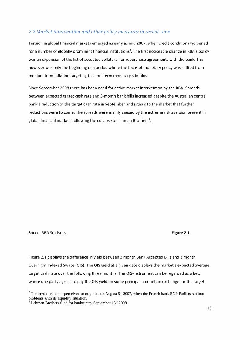
Since Se
between
bank’s re
reductio
global fin
Souce: R
Figure 2
Overnigh
target ca
where o
2 The credproblems3 Lehman
rket interv
in global fina
mber of glob
expansion of
r was only th
term inflatio
ptember 200
n expected ta
eduction of t
ons were to c
nancial mark
RBA Statistics
.1 displays th
ht Indexed S
ash rate over
ne party agr
dit crunch is p
s with its liquin Brothers file
vention an
ancial marke
bally promine
f the list of ac
he beginning
on targeting
08 there has
arget cash ra
the target ca
come. The sp
kets followin
s.
he difference
waps (OIS). T
r the followin
rees to pay th
perceived to odity situation.
ed for bankrup
d other po
ets emerged
ent financial
ccepted colla
g of a period
to short‐ter
s been need f
ate and 3‐mo
ash rate in Se
preads were
g the collaps
e in yield bet
The OIS yield
ng three mo
he OIS yield
originate on Au. ptcy Septembe
olicy measu
as early as m
institutions2
ateral for rep
where the fo
rm monetary
for active ma
onth bank bi
eptember an
mainly cause
se of Lehman
tween 3 mon
d at a given d
nths. The OI
on some prin
ugust 9th 2007
er 15th 2008.
ures in rec
mid 2007, wh2. The first no
purchase agr
ocus of mone
y stimulus.
arket interve
lls increased
nd signals to t
ed by the ex
n Brothers3.
nth Bank Acc
date displays
S‐instrumen
ncipal amou
7, when the Fr
cent time
hen credit co
oticeable cha
reements wi
etary policy
ention by the
d despite the
the market t
treme risk av
F
cepted Bills a
s the market
t can be reg
nt, in exchan
rench bank BN
onditions wo
ange in RBA’
th the bank.
was shifted f
e RBA. Sprea
Australian c
that further
version pres
igure 2.1
and 3 month
’s expected a
arded as a b
nge for the ta
NP Paribas ran
13
orsened
’s policy
This
from
ds
central
ent in
average
et,
arget
n into
14
cash rate prevailing over the following three months. Only the interest rate differential on the
principal amount is exchanged, and thus an OIS agreement has little credit risk and no liquidity
premium. 3 month Bank Accepted Bills are money market instruments issued by large banks, and the
yield comprises of both credit‐ and liquidity premium. It is evident from the development in the
graph that money market premiums first started increasing in September 2008 and continued to be
elevated until May 2009.
In comparison to other markets, the 3‐month spreads in the Australian money market have been
quite insignificant. In October 2008, when the spread reached its highest level, money market spread
was almost 400 basis points the United States. In UK, it was close to 300 basis points, and in the Euro
Area the spread was approximately 175 bps. The Australian 3‐month spread of a mere 76 basis
points is an indicator of how the Australian money market suffered less dislocation than many
others.
To calm the situation, RBA responded by intervening actively in the Australian money market. The
target cash rate was reduced every subsequent month after the initial September reduction until
money market spreads narrowed. In April 2009, the target cash rate hit a 50‐year record low of
3.00% (Business Monitor International 2010). An expected slow‐down of economic growth in
Australia justified these cuts in the target interest rate, as slack in the economy often results in low or
negative inflation rate. Cutting the interest rate is therefore a rational response, to grease the wheels
of the economy in a situation of moderation in inflationary pressure.
RBA supported the declining target cash rate by supplying more funds to the market. The list of
accepted collateral for repurchase agreements was further generously expanded in November 2008,
and the central bank also offered loans with longer maturities (6 and 12 months) to financial
intermediaries. Since the collateral pledged was required to have a maturity at least as long as the
agreement, the extended market operations had the fortunate side‐effect of improving liquidity in
the underlying market for these securities.
Another element of concern for Australian market participants was the extremely high US dollar
swap spread around the time Lehman Brothers collapsed. The RBA therefore established a USD 30
billion swap facility with the Federal Reserve in September 2008 to provide access to US dollars.
Banks and other market participants could pledge Australian dollar‐denominated securities as
collateral and get access to US dollars in return. This measure by the RBA was not undertaken
entirely to support the domestic banking sector, but also to improve the global distribution of US
dollar liq
exchang
The bett
made it
2009, an
RBA has
impleme
Figure 2
Source:
The cash
crisis. Th
2.3 Inte
Since the
should n
nation’s
policy, e
quidity. Henc
e swap line.
ter‐than‐exp
necessary fo
nd it has bee
also normal
ented to ease
.2 illustrates
RBA Statistic
h rate in the
his is a strong
ervention i
e Australian
not actively in
currency. He
ven though
ce, it was in b
ected econo
or the centra
n further rai
ised its open
e the stress i
the develop
cs
market has b
g indicator o
in the fore
dollar (AUD)
ntervene in t
ence, the ex
it has a stron
both the RBA
omic develop
l bank to rai
sed in the fo
n market ope
in domestic
pment of the
been equal t
f the success
eign exchan
) was floated
the foreign e
change rate
ng impact on
A and the Fe
pment in Aus
se target cas
ollowing mon
erations and
capital mark
e target cash
to the target
s of the Rese
nge marke
d in 1983, the
exchange ma
is neither a t
n the econom
deral Reserv
stralia and in
sh rate by 25
nths to a leve
withdrawn
kets.
rate over th
cash rate ev
erve Bank’s m
et
e consensus
arket to stee
target nor an
my. However
ve’s interest
creasing infl
5 basis points
el of 3.75% in
many of the
he past 26 mo
F
very day dur
monetary po
has been th
r the develo
n instrument
r, one situati
to establish
ationary pre
s as early as
n February 2
special facil
onths:
igure 2.2
ing the finan
licy in the pe
at the centra
pment of the
t for moneta
on where su
15
this
essure
October
2010.
ities
ncial
eriod.
al bank
e
ary
uch a
16
measure is justified is when the development of the Australian dollar diverges significantly from what
is supported by economic fundamentals and outlook (a phenomenon known as overshooting). This
was the case in the period following the Lehman Brothers bankruptcy. RBA entered the foreign
exchange market and purchased Australian dollars against US dollars. The Australian dollar was
depreciating consistently and if RBA hadn’t intervened, it would have sent signals to the Australian
real economy inconsistent with fundamentals, a trend that would be costly to reverse if market
forces alone were to be relied upon. This intervention reduced the supply of Australian dollars
available to banks, a measure that put upward pressure on market cash rate at a time when the
central bank cut the target cash rate. To counter this effect, RBA purchased securities in the open
market to increase the domestic supply of liquidity. This is called sterilized intervention.
17
CHAPTER 3. THE CREDIT MARKET
Financial intermediaries facilitate the effective distribution of financial resources in an economy. Any
dislocation in the financial system will have repercussions for the rest of the economy. Therefore, a
brief overview of how Australian banks, businesses and households experienced the global financial
crisis will be relevant to the discussion.
3.1 Banking sector
The second half of 2007 and the first three quarters of 2008 was characterised by a contraction in
Australian credit markets. Both more stringent lending standards and high interest rates made debt
conditions more problematic in the market. Short‐term funding in the Australian money market
became an issue after a series of bankruptcies or near‐bankruptcies in the worldwide banking sector.
Even with RBA’s efforts, banks as well as corporations and households were affected by this
phenomenon popularly called the credit crunch. But since the high risk aversion among investors
induced a flight from the equity market and into more safe investments, the volume of deposits in
banks increased.
In October 2008, the Australian Government introduced a range of policy measures aimed to
stabilize the credit market. One such measure was Government‐guaranteed wholesale funding (for
an additional fee). The Government also guaranteed deposits up to 1 million Australian dollars for a
period of three years.
Takàts and Tumbarello (2009) have analyzed the overall health of the Australian banking system
during the financial crisis. They find that Australian banks have been very resilient to the crisis and
their capital ratios have stayed above the Basel II regulatory requirements throughout the period. In
an international comparison, Australian banks are above average in terms of equity ratio, and around
the median with respect to deposit‐ and liquidity‐ratios4. The analysis concludes that Australian
banks are among the stronger ones in a global perspective.
Part of the fortunate outcome is due to the banks’ limited exposure to severely distressed markets,
like the American credit market. In Australian owned banks’ aggregate foreign claims, exposure to
the United States accounts for less than 10%. Furthermore, these claims are not from lending to the
4 Equity ratio = (Equity/Total assets), Deposit ratio = (Deposits/Total assets), Liquidity ratio = (Liquid assets/Total assets).
18
US household sector. The business model of Australian banks is primarily focused on domestic
lending, and the large domestic banks have not followed the international trend of expanding into
new geographical or product markets. By focusing on a more traditional banking model, Australian
banks have avoided the pitfalls of the more risky banking activities their foreign peers have recently
suffered from.
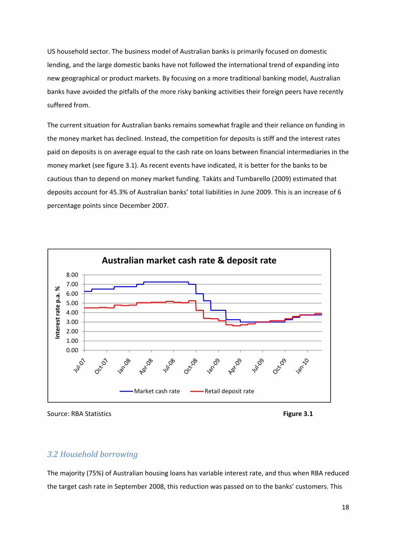
The current situation for Australian banks remains somewhat fragile and their reliance on funding in
the money market has declined. Instead, the competition for deposits is stiff and the interest rates
paid on deposits is on average equal to the cash rate on loans between financial intermediaries in the
money market (see figure 3.1). As recent events have indicated, it is better for the banks to be
cautious than to depend on money market funding. Takàts and Tumbarello (2009) estimated that
deposits account for 45.3% of Australian banks’ total liabilities in June 2009. This is an increase of 6
percentage points since December 2007.
Source: RBA Statistics Figure 3.1
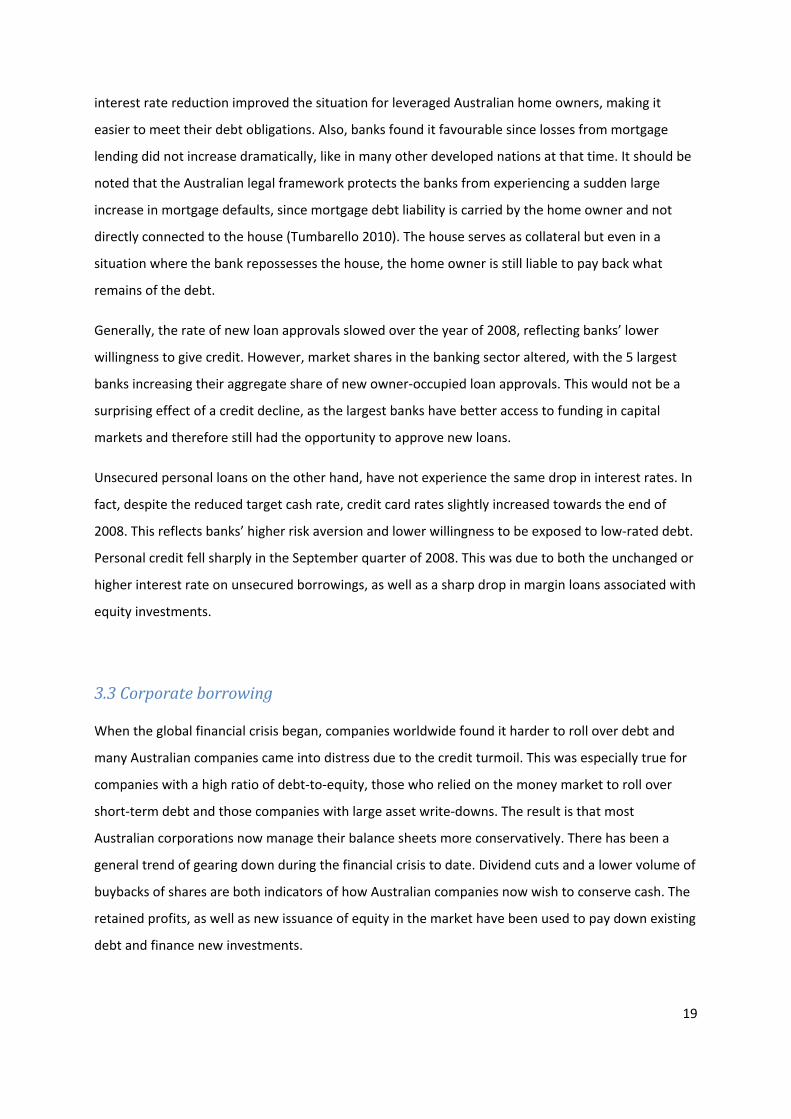
3.2 Household borrowing
The majority (75%) of Australian housing loans has variable interest rate, and thus when RBA reduced
the target cash rate in September 2008, this reduction was passed on to the banks’ customers. This
0.001.002.003.004.005.006.007.008.00
Interest ra
te p.a. %
Australian market cash rate & deposit rate
Market cash rate Retail deposit rate
19
interest rate reduction improved the situation for leveraged Australian home owners, making it
easier to meet their debt obligations. Also, banks found it favourable since losses from mortgage
lending did not increase dramatically, like in many other developed nations at that time. It should be
noted that the Australian legal framework protects the banks from experiencing a sudden large
increase in mortgage defaults, since mortgage debt liability is carried by the home owner and not
directly connected to the house (Tumbarello 2010). The house serves as collateral but even in a
situation where the bank repossesses the house, the home owner is still liable to pay back what
remains of the debt.
Generally, the rate of new loan approvals slowed over the year of 2008, reflecting banks’ lower
willingness to give credit. However, market shares in the banking sector altered, with the 5 largest
banks increasing their aggregate share of new owner‐occupied loan approvals. This would not be a
surprising effect of a credit decline, as the largest banks have better access to funding in capital
markets and therefore still had the opportunity to approve new loans.
Unsecured personal loans on the other hand, have not experience the same drop in interest rates. In
fact, despite the reduced target cash rate, credit card rates slightly increased towards the end of
2008. This reflects banks’ higher risk aversion and lower willingness to be exposed to low‐rated debt.
Personal credit fell sharply in the September quarter of 2008. This was due to both the unchanged or
higher interest rate on unsecured borrowings, as well as a sharp drop in margin loans associated with
equity investments.
3.3 Corporate borrowing
When the global financial crisis began, companies worldwide found it harder to roll over debt and
many Australian companies came into distress due to the credit turmoil. This was especially true for
companies with a high ratio of debt‐to‐equity, those who relied on the money market to roll over
short‐term debt and those companies with large asset write‐downs. The result is that most
Australian corporations now manage their balance sheets more conservatively. There has been a
general trend of gearing down during the financial crisis to date. Dividend cuts and a lower volume of
buybacks of shares are both indicators of how Australian companies now wish to conserve cash. The
retained profits, as well as new issuance of equity in the market have been used to pay down existing
debt and finance new investments.
20
The motivation behind gearing down seems to be twofold: First of all, banks have tightened their
lending standards and the bond market has been in distress, so raising new capital in the credit
market has been both difficult and costly. Secondly, due to high investor risk aversion in the market
towards the end of 2008, companies with a high gearing ratio experienced a sharper drop in their
share prices than companies with more solid balance sheets.
The net result of this balance sheet restructuring has been very clear. The aggregate gearing ratio
(book debt‐to‐equity ratio) on the Australian Stock Exchange dropped by a full 20 percentage points
to a level of 65 % in the period December 2008 – December 2009. This reduction reflects both new
issuances in the equity market, as well as repayment of loans. For some companies, the gearing ratio
has remained unchanged despite debt reductions. This is mainly due to large write‐downs in asset
value.
3.4 The Bond market
Starting in September 2008, the issuance of bonds by Australian banks slowed down and the volume
of outstanding bonds dropped. Only the highest‐rated banks found it achievable to issue new bonds
in the market, most of which were issued offshore (that is, in foreign markets). The same trend was
evident in corporate bond issuance, where large market spreads made funding in the bond market
unattractive.
A very influential series of incidents that affected the Australian bond market negatively was the
default of a number of Kangaroo bonds (bonds issued in the Australian market by foreign entities),
most notably those issued by Lehman Brothers and two Icelandic banks. Although the defaulting
bonds made up an insignificant portion of the bond market, this was the first time in history
Kangaroo bonds defaulted. It has had a powerful negative influence on Australian investors’ appetite
for bonds issued by foreigners.
Towards the end of 2009, banks’ issuance of bonds picked up, although a majority was issued
offshore. Another trait signalling a better outlook for Australian banks is the fact that a majority of
the bonds issued was not guaranteed, since this was a more affordable source of funding than the
Government guaranteed funding scheme. This would not be the case if the extreme risk aversion
seen towards the end of 2008 was still affecting market participants. Reduced risk aversion has also
enabled non‐financial firms to issue bonds in the market in this period.
21
3.5 Residential MortgageBacked Securities (RMBS)
The American Sub‐Prime product has become the scapegoat of the financial crisis. All over the world,
similar products have come into severe distress simply due to their resemblance to the American
version. Residential Mortgage‐Backed Securities (RMBS) is a good example of this effect. These are
sold to the market by Australian banks, but unlike the Sub‐Prime products, they are made from
highly rated residential mortgages. Before September 2008, offshore demand for this product was
high, reflecting the relatively high quality of Australian mortgages.
Tension in the market for these products intensified towards the end of 2008. The Australian central
bank resolved domestic tension by including these and other securities in distressed markets on the
list of accepted collateral for repurchase agreements. After September 2008, there was a large drop
in issuance of this type of security. However, conditions improved in 2009, and towards the end of
the year there was a new issue of RMBS in the Australian market. The Australian Office of Financial
Management (AOFM) was the biggest purchaser of this product. AOFM, a specialist Government
agency, invests in these products to “maintain competition in lending for housing in Australia”.
In total, the Australian credit market has remained more stable than in many other countries.
CHAP
Some tu
experien
of solid e
markets
volatility
factor of
Source:
Figure 4
Exchang
Septemb
econom
index fo
on world
2009, an
sector.
PTER 4.
rbulence in t
nced a sharp
earnings and
at the time.
y in the Austr
f scaring inve
RBA Statistic
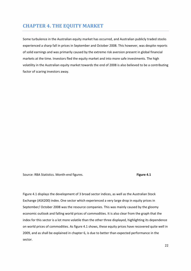
.1 displays th
e (ASX200) i
ber/ October
ic outlook an
r this sector
d prices of co
nd as shall be
THE EQ
the Australia
fall in prices
d was primar
Investors fle
ralian equity
estors away.
cs. Month‐en
he developm
ndex. One se
r 2008 was t
nd falling wo
is a lot more
ommodities.
e explained i
QUITY M
an equity ma
s in Septemb
rily caused by
ed the equity
y market tow
nd figures.
ment of 3 bro
ector which
he resource
orld prices of
e volatile tha
As figure 4.1
n chapter 6,
MARKET
arket has occ
ber and Octo
y the extrem
y market and
wards the end
oad sector in
experienced
companies.
f commoditie
an the other
1 shows, the
is due to be
curred, and A
ber 2008. Th
me risk aversi
d into more
d of 2008 is a
dices, as wel
d a very large
This was ma
es. It is also c
three display
ese equity pr
tter than exp
Australian pu
his however,
ion present i
safe investm
also believed
F
ll as the Aust
e drop in equ
ainly caused
clear from th
yed, highligh
ices have rec
pected perfo
ublicly traded
was despite
n global fina
ments. The hi
d to be a con
igure 4.1
tralian Stock
uity prices in
by the gloom
he graph that
hting its depe
covered quit
ormance in t
22
d stocks
e reports
ancial
gh
ntributing
k
my
t the
endence
te well in
he
23
As illustrated in figure 4.1, Australian banks and other financial intermediaries did not experience the
same extreme equity price drop as the resource sector. As discussed in the previous chapter,
Australian banks have proven to be robust. Asset write‐downs have been limited, and Australian
banks have generally had very insignificant exposure to the U.S Sub‐Prime market (Tumbarello 2010).
A large part of their balance sheet assets can be classified as low‐risk domestic loans, and the five
largest Australian banks have maintained their S&P credit rating of AA throughout the financial crisis.
However, Australian banks’ foreign operations have shown low profitability also throughout 2009.
The majority of the foreign operations are located in Great Britain and New Zealand, two countries
which have experienced more economic difficulties than Australia.
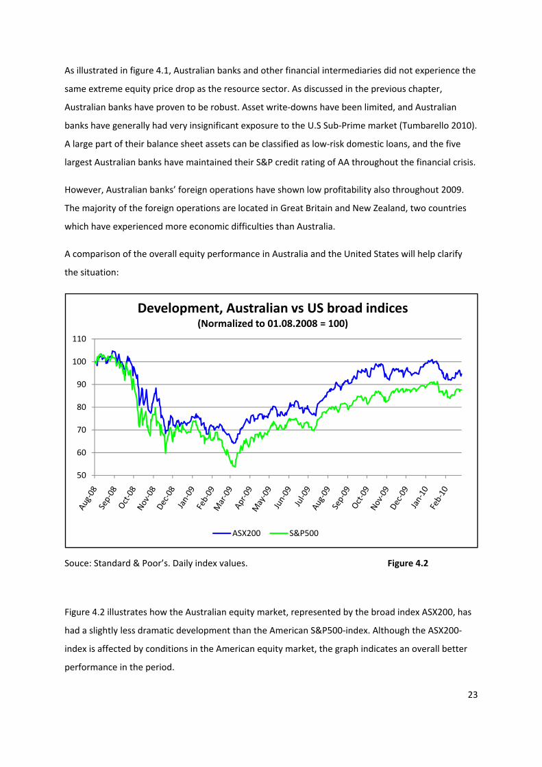
A comparison of the overall equity performance in Australia and the United States will help clarify
the situation:
Souce: Standard & Poor’s. Daily index values. Figure 4.2
Figure 4.2 illustrates how the Australian equity market, represented by the broad index ASX200, has
had a slightly less dramatic development than the American S&P500‐index. Although the ASX200‐
index is affected by conditions in the American equity market, the graph indicates an overall better
performance in the period.
50
60
70
80
90
100
110
Development, Australian vs US broad indices(Normalized to 01.08.2008 = 100)
ASX200 S&P500
24
In the September‐quarter 2009, Australian banks raised 7,5 billion Australian dollars in the equity
market. This comes to show that investors’ demand for bank equity securities is returning. Other
large, listed corporations have also been able to issue new equity in the Australian market during the
crisis. In the first quarter of 2009, private non‐financial companies raised over 18 billion Australian
dollars in the equity market. This is nearly twice as much as the amount of equity raised the first
quarter of 2008 (Takàts and Tumbarello 2009). The purpose of the newly raised equity has mainly
been debt repayment and new investments.
Towards the end of 2009, there was an increase in Initial Public Offerings (IPOs) in the Australian
market. IPOs have been subdued since July 2008 and the recent increase signals improvement in the
Australian equity market.
25
CHAPTER 5. DOMESTIC DEMAND
Domestic consumption fell during the first half of 2008, as the economic outlook deteriorated and a
contraction in credit markets resulted in high interest rates on consumer credit.
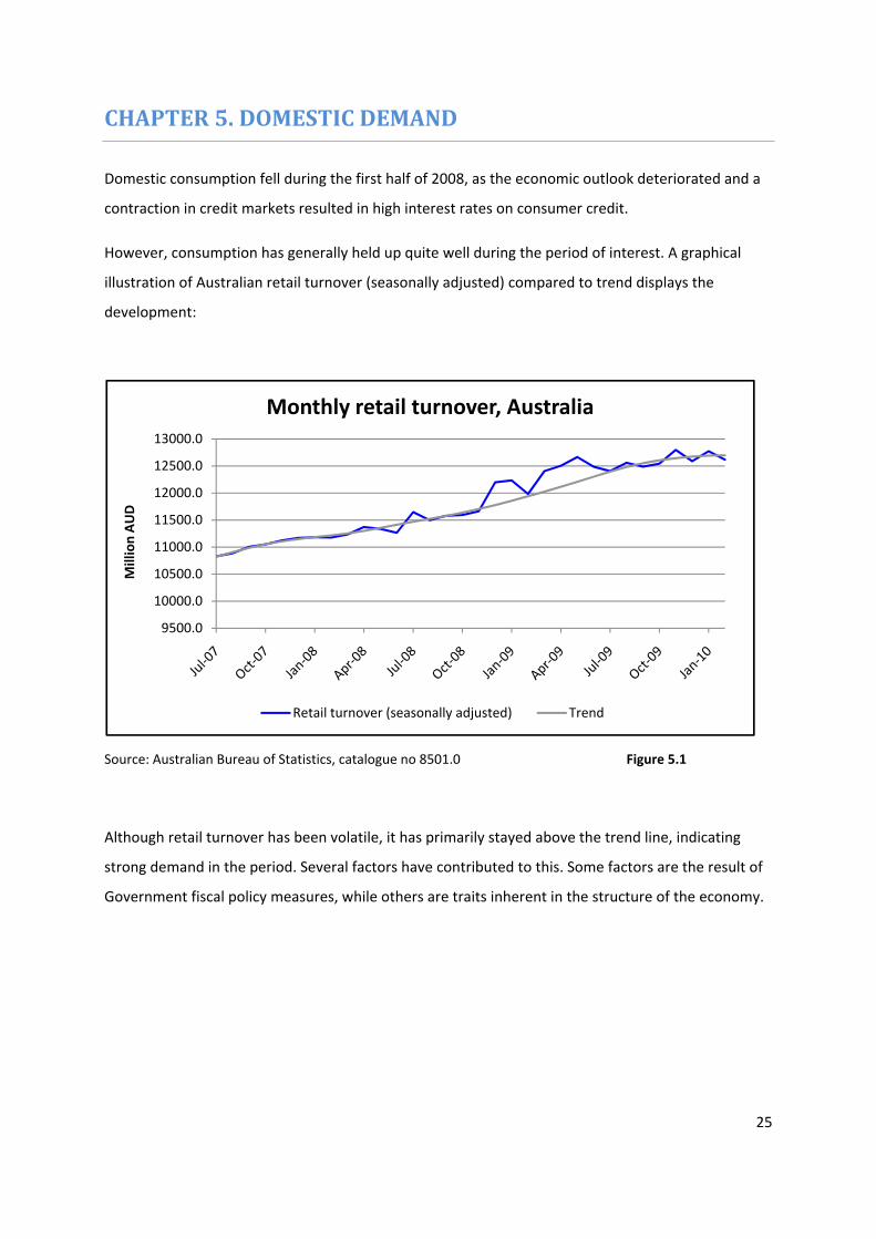
However, consumption has generally held up quite well during the period of interest. A graphical
illustration of Australian retail turnover (seasonally adjusted) compared to trend displays the
development:
Source: Australian Bureau of Statistics, catalogue no 8501.0 Figure 5.1
Although retail turnover has been volatile, it has primarily stayed above the trend line, indicating
strong demand in the period. Several factors have contributed to this. Some factors are the result of
Government fiscal policy measures, while others are traits inherent in the structure of the economy.
9500.0
10000.0
10500.0
11000.0
11500.0
12000.0
12500.0
13000.0
Million AUD
Monthly retail turnover, Australia
Retail turnover (seasonally adjusted) Trend
26
5.1 Fiscal policy and stimulus packages
The Australian Government has undertaken several fiscal policy measures since the onset of the
crisis. These measures intend to create jobs and stimulate domestic demand. A number of
construction projects funded by the Government have recently been undertaken. The majority of
these projects focus on upgrading school buildings, public housing, and more recently also
infrastructure.
Another example of a fiscal policy measure aimed to stimulate domestic consumption is a program
called Household Stimulus Package. This program was announced by the Australian Government on
February 3rd 2009, and was aimed to assist low‐ to middle income families during the economic
downturn. The financial aid comprised of a one‐time payment of approximately 1000 Australian
dollars per household, as well as additional funds for families with young children or other financial
strains (Australian Government Centrelink 2009). In aggregate, the Household Stimulus Package has
cost the Government 21 billion Australian dollars.
Professor Andrew Leigh (2009) has estimated the effect of the Australian Household Stimulus
Package. He found that approximately 40% of the Australian stimulus package recipients reported to
have spent it. This is twice as much as for the American 2008 tax rebate programme. Leigh points at
one possible explanation for this; recipients are more likely to spend when the stimulus package is
presented as a bonus rather than a reduction in tax payment. Leigh’s survey indicates that how a
stimulus measure is presented will dictate its effectiveness.
The Australian Government’s fiscal policy measures have been criticized for their large costs relative
to the expected benefits. American economist Russel Roberts (2008) refers to consumer stimulus
packages it the following statement: “It’s like taking a bucket of water from the deep end of a pool
and dump it into the shallow end”. In classical economic theory, the Mundell‐Fleming model predicts
fiscal policy to be completely ineffective when the nation operates with a flexible exchange rate
(Gärtner 2006). In the model, Government spending increases demand for domestic currency,
effectively causing the exchange rate to appreciate. In this scenario, a crowding out effect occurs,
where increased public spending pushes down private spending (most notably exports). However,
the model describes the ceteris paribus effect of fiscal policy in an open economy with floating
exchange rate. The situation in Australia was that monetary policy was simultaneously eased to
counteract the effects of the crisis.
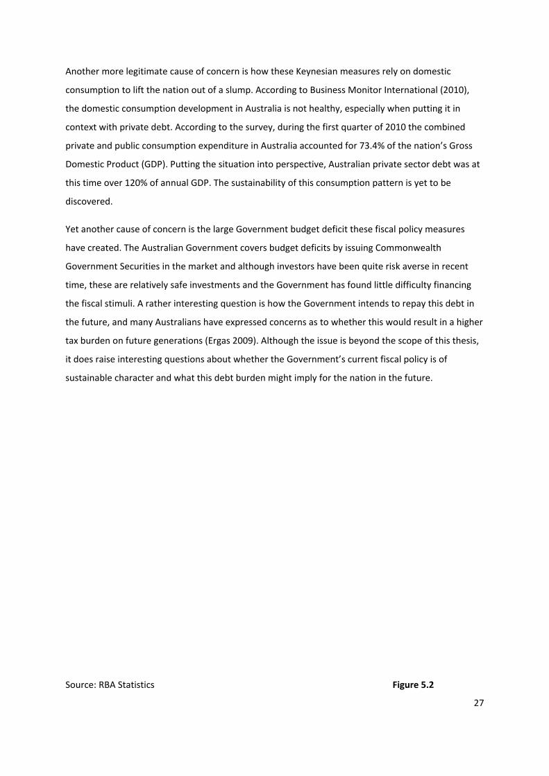
Another
consump
the dom
context w
private a
Domesti
this time
discover
Yet anot
have cre
Governm
time, the
the fisca
the futu
tax burd
it does r
sustaina
Source:
more legitim
ption to lift t
mestic consum
with private
and public co
ic Product (G
e over 120%
red.
ther cause of
eated. The Au
ment Securit
ese are relat
al stimuli. A r
re, and many
en on future
aise interest
ble characte
RBA Statistic
mate cause o
the nation ou
mption deve
debt. Accor
onsumption
GDP). Putting
of annual GD
f concern is t
ustralian Gov
ies in the ma
ively safe inv
ather intere
y Australians
e generation
ting question
er and what t
cs
of concern is
ut of a slump
lopment in A
ding to the s
expenditure
g the situatio
DP. The sust
the large Gov
vernment co
arket and alt
vestments an
sting questio
s have expre
s (Ergas 200
ns about whe
this debt bur
how these K
p. According
Australia is n
survey, durin
in Australia
on into persp
ainability of
vernment bu
overs budget
though inves
nd the Gove
on is how the
essed concer
9). Although
ether the Go
rden might im
Keynesian m
to Business
ot healthy, e
ng the first qu
accounted f
pective, Aust
this consum
udget deficit
t deficits by i
stors have be
rnment has
e Governme
ns as to whe
h the issue is
overnment’s
mply for the
easures rely
Monitor Inte
especially wh
uarter of 201
for 73.4% of
ralian privat
mption patter
t these fiscal
ssuing Comm
een quite risk
found little d
nt intends to
ether this wo
beyond the
current fisca
nation in th
F
y on domesti
ernational (2
hen putting i
10 the comb
the nation’s
e sector deb
rn is yet to be
policy meas
monwealth
k averse in re
difficulty fina
o repay this d
ould result in
scope of this
al policy is of
e future.
igure 5.2
27
c
2010),
t in
bined
Gross
bt was at
e
ures
ecent
ancing
debt in
a higher
s thesis,
f
28
Dungey (2001) has analyzed international shocks and the role of domestic policy in Australia. He
found that Australia has dealt well with previous global disturbances such as the Asian crisis in 1997
primarily due to sound domestic policy responses. The analysis also highlights the importance of
allowing the nation’s floating currency to act as a shock absorber. Conclusively, Dungey holds the
perception that the worst policy response would be to remain passive. Even though a small, open
economy like Australia is widely influenced by external forces, domestic monetary and fiscal policy
has an impact on the outcome when an external shock hits the economy.
5.2 Other factors of relevance
5.2.1 Asset prices recovered
One of the most influential events leading to the financial crisis was the implosion of the house price
bubble in USA. Combined with the stock market crash, many Americans saw their household wealth
diminish in a short period of time. The situation in Australia however, has been very different. House
prices dropped in 2008, but they quickly recovered. Australia is a country with remarkably high
population growth, with 1.53% annual growth in 2007 – compared to 0.96% in the United States
(OECD Factbook 2009). This magnitude of growth is primarily caused by a high level of immigration.
The population growth creates pressure in the housing market, making speculative bubbles a
phenomenon less prone to occur. House prices started rising again in 2009 and is currently at a
higher level than the previous peak. The Australian equity market has also recovered from 2008’s
sharp price drop. Rising house‐ and equity prices add to household wealth, and this has supported
consumer confidence and helped stabilize consumption.
The net effect of fiscal and monetary policy measures (stimulus packages and lower interest rates) is
that Australians have enjoyed a higher real disposable income than prior to the financial crisis. This
has supported consumer confidence and helped domestic demand stay elevated throughout the
period.
5.2.2 Unemployment rate stable
The financial crisis has had a mild negative effect on domestic production (which will be discussed in
next chapter). A somewhat lower domestic production would normally result in layoffs and a higher
29
unemployment rate. But the Australian labour market is of a unique character, something quite
different from labour markets in many other developed countries.
The fact is that the unemployment rate in Australia has been flat and steady at 5.75 % since June
2009. From mid 2007 to end 2008, the unemployment rate fluctuated around a level of 4.25 %. Most
layoffs have occurred in the financial sector (Business Monitor International 2010). With a high level
of immigration, this might seem counterintuitive. However, it does have a simple explanation. Firstly,
the participation rate has fallen moderately. And secondly, the Australian labour market is
abnormally flexible in the sense that when demand for labour dropped, employees agreed to work
fewer hours per week and in return keep their job. Although this has a negative effect on domestic
disposable income, it does not seem to have affected consumer confidence in the same scale as in
comparable countries with a high or rising unemployment rate. The high level of flexibility stems
from a comprehensive deregulation regime initiated by the Liberal‐National Coalition Government
(1996‐2007), which restricted union involvement in the workplace and liberalized constraints on
hiring and firing employees (Business Monitor International 2010). The current Government has
suggested a reintroduction of collective bargaining, only to be met by a heated debate about how
this will increase the unemployment rate and make Australia less competitive internationally. A
flexible labour market is yet another trait that makes the Australian economy very robust and
capable of handling global economic disturbances.
5.2.3 Financial markets calmed
As previously covered, Australian financial markets calmed down in mid 2009. Spreads in credit
markets narrowed, Australian firms increased their balance sheets’ robustness and the extreme risk
aversion evaporated. The effect on domestic demand is difficult to infer precisely. However,
according to the Australian Financial Markets Association (2010), “a competitive, resilient and
efficient financial system is central to a successful economy”. With financial markets moving back
towards equilibrium, it is believed that this development has had a positive psychological effect on
consumer confidence.
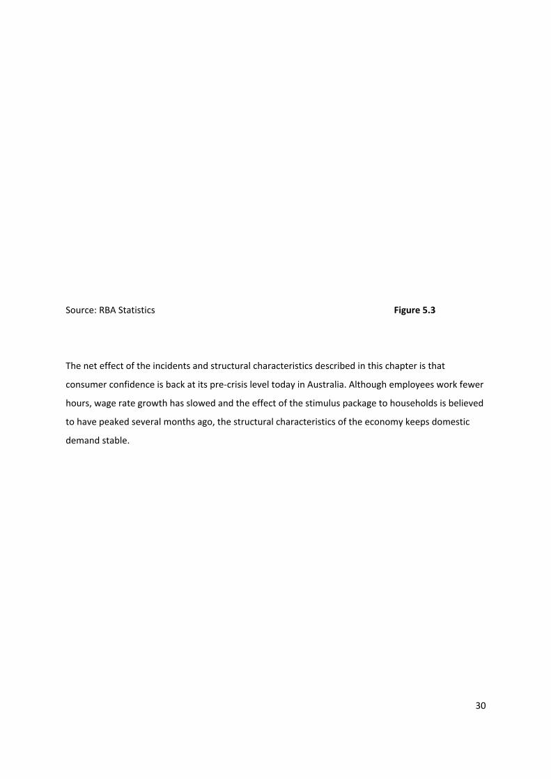
Source:
The net
consume
hours, w
to have
demand
RBA Statistic
effect of the
er confidenc
wage rate gro
peaked seve
stable.
cs
e incidents an
e is back at i
owth has slow
eral months a
nd structura
its pre‐crisis
wed and the
ago, the stru
l characteris
level today i
e effect of the
ctural chara
tics describe
in Australia.
e stimulus pa
cteristics of
F
ed in this cha
Although em
ackage to ho
the econom
igure 5.3
apter is that
mployees wo
ouseholds is
y keeps dom
30
ork fewer
believed
mestic
31
CHAPTER 6. INTERNATIONAL CONDITIONS AND DOMESTIC PRODUCTION
6.1 The global environment
Around the turn of the year 2008/2009 most advanced and many developing economies were
struggling with the effects of the financial crisis. As a consequence, international trade plummeted.
According to WTO’s International Trade Statistics (2009), total world merchandise exports fell by
over 30% the first quarter of 2009, compared to the first quarter of 2008.
Part of the slowdown can also be attributed to the inventory cycle, a phenomenon where companies
keep a large volume of inventory during good times, while scaling down their stock of inventory in
economic downturns. The rationale behind this behaviour is to avoid write‐downs on goods they are
not able to sell, as demand and often also prices fall. However, the recent global recession has had a
second attribute which makes it rational to believe that the inventory cycle has been a driving force
for falling trade: The credit crunch. The difficulties many companies have experienced with their
access to lending has forced many to reduce their level of tied‐up capital in order to meet financial
demands.
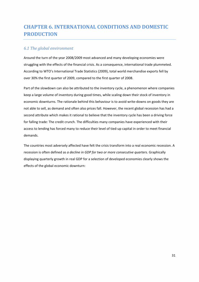
The countries most adversely affected have felt the crisis transform into a real economic recession. A
recession is often defined as a decline in GDP for two or more consecutive quarters. Graphically
displaying quarterly growth in real GDP for a selection of developed economies clearly shows the
effects of the global economic downturn:
32
Source: RBA Statistics Figure 6.1
Domestic activity in these countries has slowed and domestic demand contracted. The Australian
economy has done quite well despite the unfavourable situation of an outside world in recession.
When looking at the development in quarterly GDP for Australia, only the December 2008‐ quarter
exhibits negative growth. Hence, according to the definition, Australia has been able to avoid a
recession in the domestic economy altogether.
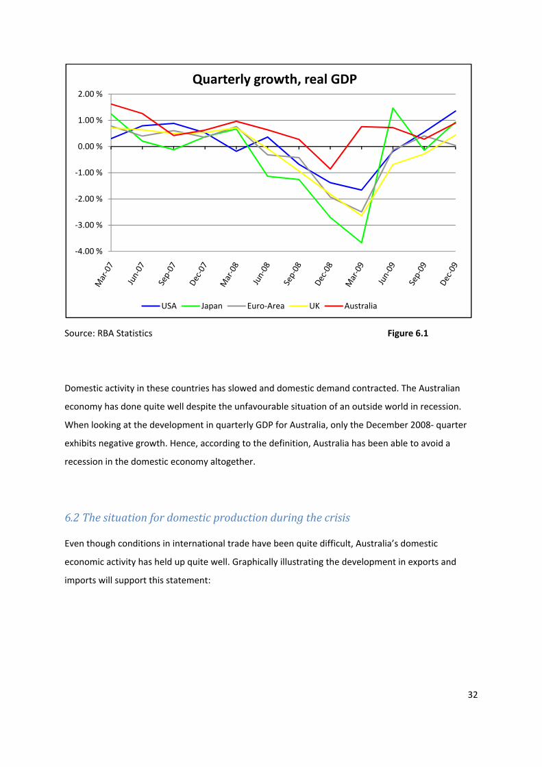
6.2 The situation for domestic production during the crisis
Even though conditions in international trade have been quite difficult, Australia’s domestic
economic activity has held up quite well. Graphically illustrating the development in exports and
imports will support this statement:
‐4.00 %
‐3.00 %
‐2.00 %
‐1.00 %
0.00 %
1.00 %
2.00 %Quarterly growth, real GDP
USA Japan Euro‐Area UK Australia
Source:
Figures o
measure
As figure
througho
due to d
can be a
products
pattern w
6.3 The
Even tho
than oth
times, so
income e
5 Merchan
RBA Statistic
originally sta
ed in current
e 6.2 displays
out the perio
omestic dem
ttributed to
s and major t
will be highli
e export se
ough the glob
hers. One rea
ome goods e
elasticity of m
ndise is a term
cs.
ated in millio
t prices.
s, Australian
od, without a
mand being r
the compos
trading partn
ighted.
ector
bal economi
ason is that e
enjoy a relati
manufacture
m employed in
n AUD (seas
merchandis
any dramatic
resilient to th
ition of Aust
ners. In the f
c contractio
even though
vely stable d
ed exports is
n international
onally adjust
se5 exports a
c decline. On
he external s
tralia’s intern
following, so
n has affecte
aggregated
demand. Res
higher than
l trade, referri
ted),
nd imports h
ne reason for
shock. Other
national trad
ome characte
ed most nati
world trade
search on wo
the income
ing to trade in
F
have develop
r this is as pr
explanation
de, both in re
eristics of Au
ons, some h
has fallen d
orld trade ind
elasticity of
(tangible) go
igure 6.2
ped rather sm
reviously disc
ns for this ou
egard to expo
ustralia’s trad
ave suffered
ramatically i
dicates that t
total merch
ods (IMF 20033
moothly
cussed
tcome
ort
de
d less
n recent
the
andise
09).
34
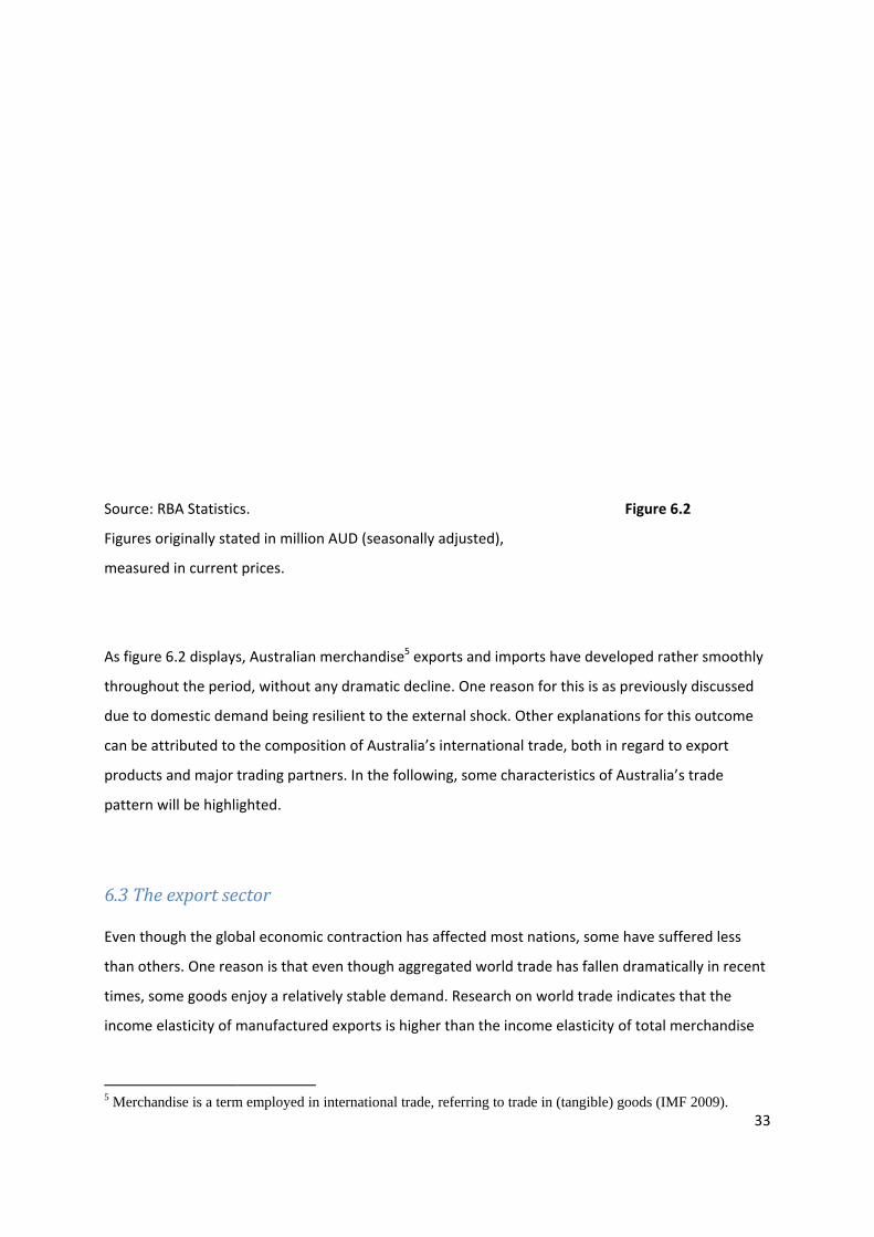
exports6 (WTO International Trade Statistics 2009). It naturally follows that economies primarily
exporting commodities generally fare better than those exporting manufactured goods in a global
contraction of trade. The composition of Australia’s exports is displayed in figure 6.3:
Source: Australian Bureau of Statistics, catalogue no. 5368.0 Figure 6.3
Resources, defined as minerals and fuels7, make up almost half of the nation’s exports. Figure 6.3
illustrates how commodities in total make up almost two thirds of Australian exports.
Due to the composition of export products, Australia has not experienced the dramatic decline in
export volumes the way many other developed economies have. Commodity prices began falling in
the second half of 2008 due to expectations of slower global growth in 2009. But in May 2009, the
downward trend reversed and prices began slowly increasing again. This is a sign of global recovery,
and for Australia the effect can be seen in increased equity prices for commodity producers, as well
as increased investment in the sector.
6 1960-2008 average income elasticity for manufactures = 2.1, income elasticity of total merchandise =1.7 7 This is the definition employed by the Australian Government Department of Foreign Affairs and Trade (2009).
Rural. 10.3 %
Resources. 44.8 %
Manufactures. 15.4 %
Gold. 6.1 %
Other Goods. 4.6 %
Services. 18,7 %
Australia's composition of exports 2008-09
Source:
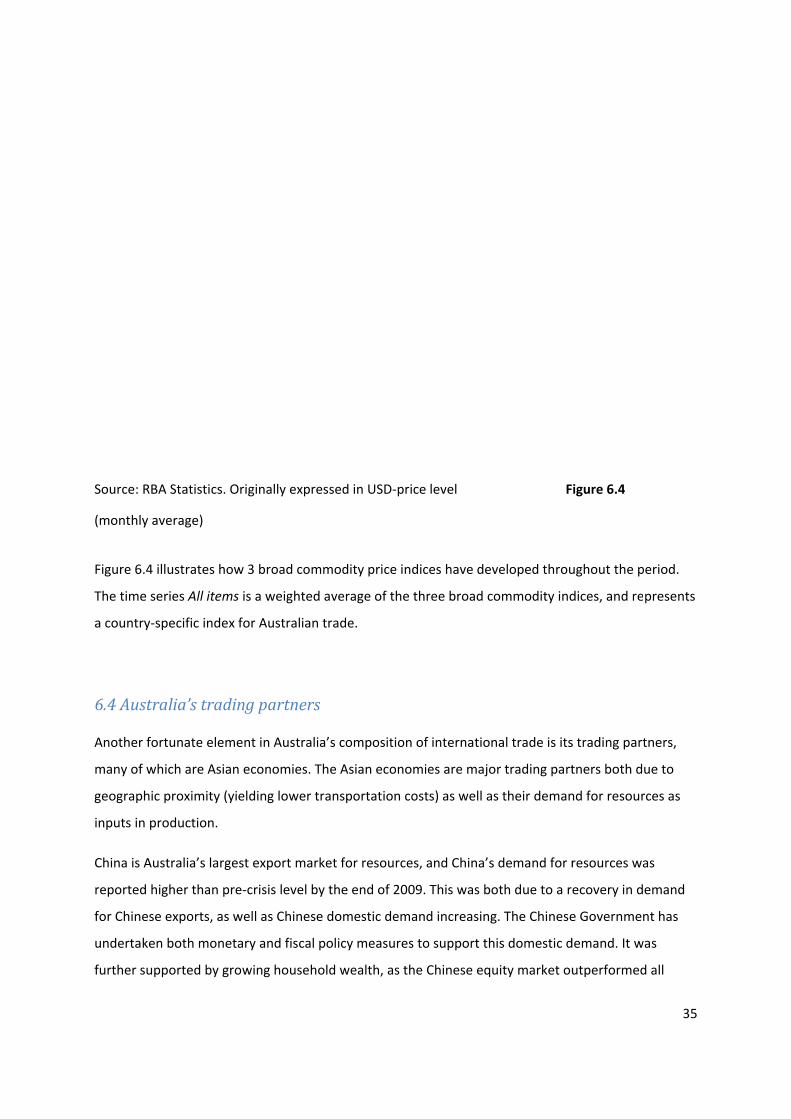
(monthly
Figure 6
The time
a countr
6.4 Aus
Another
many of
geograp
inputs in
China is
reported
for Chine
undertak
further s
RBA Statistic
y average)
.4 illustrates
e series All it
ry‐specific ind
stralia’s tra
fortunate e
which are A
hic proximity
n production
Australia’s la
d higher than
ese exports,
ken both mo
supported by
cs. Originally
how 3 broa
tems is a wei
dex for Aust
ading part
lement in Au
Asian econom
y (yielding lo
.
argest expor
n pre‐crisis le
as well as Ch
onetary and f
y growing ho
expressed in
d commodit
ghted averag
ralian trade.
tners
ustralia’s com
mies. The Asi
ower transpo
rt market for
evel by the e
hinese dome
fiscal policy
ousehold we
n USD‐price
y price indic
ge of the thr
mposition of
an economie
ortation cost
r resources, a
end of 2009.
estic demand
measures to
alth, as the C
level
es have deve
ree broad co
internationa
es are major
s) as well as
and China’s d
This was bot
d increasing.
o support this
Chinese equi
F
eloped throu
mmodity ind
al trade is its
r trading part
their deman
demand for r
th due to a r
The Chinese
s domestic d
ity market ou
igure 6.4
ughout the p
dices, and re
s trading part
tners both d
nd for resour
resources wa
ecovery in d
e Governmen
demand. It w
utperformed
35
period.
presents
tners,
ue to
rces as
as
emand
nt has
was
d all
others, r
export se
Other ec
similar to
dislocati
system h
general s
Source:
6.5 The
The third
relations
ratio bet
Septemb
the majo
8 The Hanby 74% in
rising by ove
ector immen
conomies in
o before the
on in their fi
has been an
stability of th
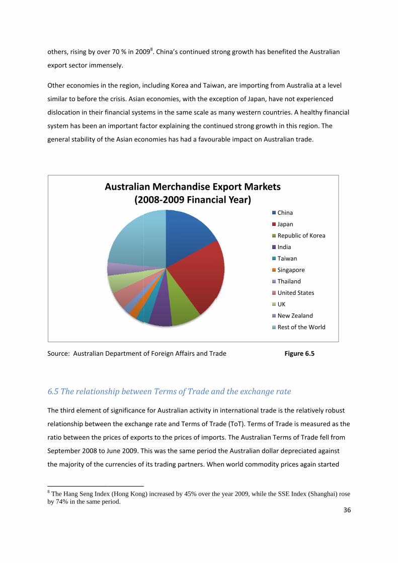
Australian D
e relations
d element of
ship between
tween the pr
ber 2008 to J
ority of the c
ng Seng Indexn the same pe
A
r 70 % in 200
nsely.
the region, i
e crisis. Asian
inancial syste
important fa
he Asian eco
Department o
ship betwee
f significance
n the exchan
rices of expo
June 2009. T
currencies of
x (Hong Kongeriod.
Australia(20
098. China’s c
ncluding Kor
n economies,
ems in the sa
actor explain
onomies has
of Foreign Af
en Terms o
e for Australi
nge rate and
orts to the pr
This was the s
f its trading p
g) increased by
n Merch008‐2009
continued st
rea and Taiw
, with the ex
ame scale as
ning the cont
had a favour
ffairs and Tra
of Trade a
ian activity in
Terms of Tr
rices of impo
same period
partners. Wh
y 45% over th
handise E9 Financ
trong growth
wan, are impo
ception of Ja
s many weste
tinued strong
rable impact
ade
nd the exc
n internation
ade (ToT). Te
orts. The Aus
the Australi
hen world co
he year 2009, w
Export Mial Year)
h has benefit
orting from A
apan, have n
ern countrie
g growth in t
t on Australia
F
hange rate
nal trade is th
erms of Trad
tralian Term
ian dollar de
mmodity pri
while the SSE
Markets
Chin
Japa
Rep
Indi
Taiw
Sing
Tha
Unit
UK
New
Rest
ted the Austr
Australia at a
not experienc
s. A healthy
this region. T
an trade.
igure 6.5
e
he relatively
de is measure
ms of Trade fe
preciated ag
ices again sta
E Index (Shan
na
an
ublic of Korea
a
wan
gapore
iland
ted States
w Zealand
t of the World
36
ralian
a level
ced
financial
The
robust
ed as the
ell from
gainst
arted
ghai) rose
a
d
37
rising in mid 2009 (causing the Australian ToT to rise), the Australian dollar began appreciating. This
yields a very fortunate effect on Australian real economy. Australian resource exporters benefit from
the co‐movement in the two economic indicators. They report profits in Australian dollars, and these
profits have remained relatively stable despite high volatility in international markets. The net effect
of the relationship between the exchange rate and ToT is that Australian domestic production has
been more stable than in many other countries.
6.6 Current climate for domestic production
The favourable situation for Australian companies in international trade has helped production stay
above previously expected levels. Furthermore, there has been a restructuring in the economy
towards the commodity sector. This has been evident in the level of investment in the sector.
Generally, 2009 investment has been high relative to GDP in Australia. And the resource sector is the
one investing the most, partially due to the pick‐up in demand in Asia. Restructuring in the economy
may impose challenges for the nation, as capital and labour must shift from other sectors. However,
the Australian labour market has proven to be very flexible, and the high rate of immigration will
help ease the pressure created in the economy from this restructuring.
In a small, open economy like Australia, international trade has a strong impact on its economic
performance. In this chapter, factors affecting domestic production have been addressed, primarily
in the context of international trade. The net effect of these factors has been less slack in the
economy than previously expected. This has added to inflationary pressure and is reported as one of
the reasons the central bank increased the target cash rate as early as October 2009.
38
CHAPTER 7. EXCHANGE RATE DEVELOPMENTS
The exchange rate is the one factor linking all the previously described markets together. It is also a
very strong link relating the nation to the outside world. Therefore, the behaviour of the Australian
dollar during the period in question will be addressed in this chapter.
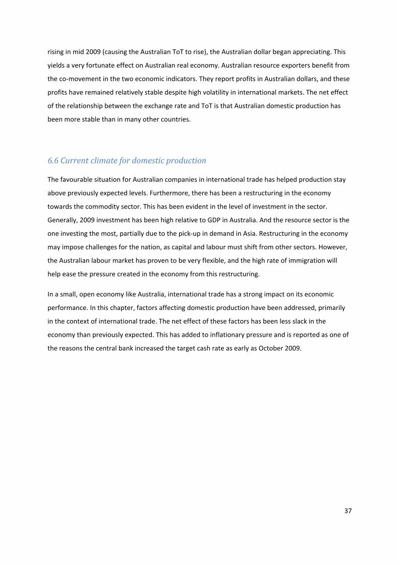
7.1 The Australian dollar – relative to what?
The Australian dollar was floated in 1983.There are two measures of the Australian dollar commonly
used: The Australian dollar against the US dollar, and the Australian dollar against the Trade
Weighted Index (TWI). The latter is not a currency, but rather an index based on the conversion value
of Australian dollars relative to the currencies of Australia’s most important trading partners. Each
bilateral exchange rate included in the index is assigned a weight reflecting its relative importance to
Australian international trade. Australian dollar against the Trade Weighted Index is thus the
multilateral or effective exchange rate (Moosa 2006). It captures the strength of the Australian dollar
on a broader basis than the bilateral exchange rate USD/AUD does. As of October 2009, the
composition of the index is as shown in table 7.1:
Table 7.1: TWI WEIGHTS (October 2009) Currency Weight (%) Chinese renminbi 18.56Japanese yen 17.12European euro 10.44United States dollar 8.98South Korean won 6.26United Kingdom pound sterling 4.99Singapore dollar 4.61Indian rupee 4.26Thai baht 3.82New Zealand dollar 3.79New Taiwan dollar 2.97Malaysian ringgit 2.93Indonesian rupiah 2.27Vietnamese dong 1.37United Arab Emirates dirham 1.34Papua New Guinea kina 1.12Hong Kong dollar 1.12Canadian dollar 0.96South African rand 0.81Saudi Arabian riyal 0.77Swiss franc 0.76Swedish krona 0.73
39
Table 7.1 confirms that several of Australia’s most important trading partners are located in the
Asian‐Pacific region. Furthermore, the table indicates which other economies (and their respective
conditions during the financial crisis) might have been the most influential to the Australian dollar in
the period of distress.
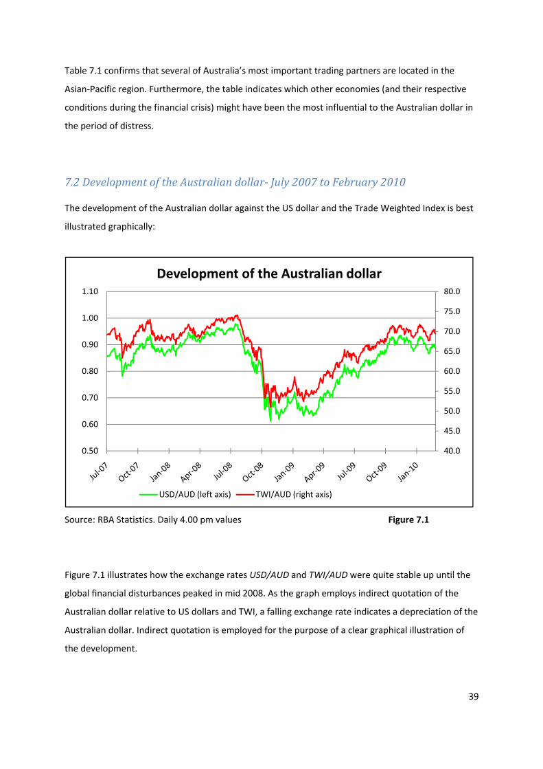
7.2 Development of the Australian dollar July 2007 to February 2010
The development of the Australian dollar against the US dollar and the Trade Weighted Index is best
illustrated graphically:
Source: RBA Statistics. Daily 4.00 pm values Figure 7.1
Figure 7.1 illustrates how the exchange rates USD/AUD and TWI/AUD were quite stable up until the
global financial disturbances peaked in mid 2008. As the graph employs indirect quotation of the
Australian dollar relative to US dollars and TWI, a falling exchange rate indicates a depreciation of the
Australian dollar. Indirect quotation is employed for the purpose of a clear graphical illustration of
the development.
40.0
45.0
50.0
55.0
60.0
65.0
70.0
75.0
80.0
0.50
0.60
0.70
0.80
0.90
1.00
1.10
Development of the Australian dollar
USD/AUD (left axis) TWI/AUD (right axis)
40
Furthermore, figure 7.1 illustrates how the development of the Australian dollar against each of the
reciprocating currencies is similar in direction and magnitude. This is not entirely coincidental, as the
US dollar is part of the Trade Weighted Index with a weight of approximately 9%. Furthermore, the
Chinese renminbi is pegged to USD (Twome 2009), and thus the American currency has a strong
influence on the Australian Trade Weighted Index.
In figure 7.1, it is evident how the Australian dollar depreciated consistently against the currencies of
its trading partners from July 2008 to May 2009. From this point up until year end 2009, the
Australian dollar again appreciated. This was the same period of time where world commodity prices
fell, and then recovered.
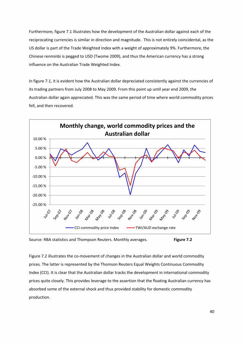
Source: RBA statistics and Thompson Reuters. Monthly averages. Figure 7.2
Figure 7.2 illustrates the co‐movement of changes in the Australian dollar and world commodity
prices. The latter is represented by the Thomson Reuters Equal Weights Continuous Commodity
Index (CCI). It is clear that the Australian dollar tracks the development in international commodity
prices quite closely. This provides leverage to the assertion that the floating Australian currency has
absorbed some of the external shock and thus provided stability for domestic commodity
production.
‐25.00 %
‐20.00 %
‐15.00 %
‐10.00 %
‐5.00 %
0.00 %
5.00 %
10.00 %
Monthly change, world commodity prices and the Australian dollar
CCI commodity price index TWI/AUD exchange rate
41
This stabilizing effect also applies to inflation. Since a large part of Australian business activity is
related to commodity production in some way, rising world commodity prices will result in increased
business activity, and thus inflationary pressure in Australia. An exchange rate that simultaneously
appreciates will help modify this inflationary pressure, since the domestic prices of imported goods
fall. By the same analogy, falling world commodity prices will ease inflationary pressure from
Australian production. If this development is accompanied by a depreciating Australian dollar, the
price of imports rise and inflation in the sector of tradable goods increase. Therefore, the
relationship helps stabilize both production and inflation in the Australian economy.
The relationship between the Australian dollar and commodity prices has been analyzed extensively,
and will be further discussed in Part Two, where an exchange rate model will be presented.
42
CHAPTER 8. SUMMARY, PART ONE
Part One has focused on conditions in Australian markets during the period of financial distress; July
2007 – February 2010. The aim of Part One is to provide an overview of the macroeconomic situation
for the nation. This overview yields the impression of a nation both prepared for and well fit to battle
the effects of a global recession.
There are several reasons why Australia dealt so well with the crisis. Both Government policy
measures and the inherent flexibility in the labour market have contributed to keeping domestic
supply and demand stable, presumably by affecting the overall psychological comprehension of the
situation. The monetary authorities and the Government have signalled their dedication and strength
to keeping the economy afloat. If these signals had not been regarded as credible, the effectiveness
of the measures is questionable. However, the Australian population has displayed faith in the
authorities and a positive outlook on the situation.
Another element of significance is Australia’s position in international trade. Both trading partners
and composition of exports have affected the economy in a positive manner. Perhaps the most
striking and unique characteristic of Australia’s international trade is the perceived strong
relationship between the Australian dollar and Terms of Trade. This relationship has provided
stability for domestic production, predominantly in the commodity sector. Although the relationship
does not benefit domestic non‐commodity related production, flexibility in the labour market (well
supported by high immigration) makes restructuring smoother and with less friction than for many
other nations.
The literary study leading up to this presentation has had the added benefit of highlighting which
economic indicators one should pay close attention to in an empirical analysis. Constructing a
descriptive presentation provides insight and clues to underlying structural relationships in the
economy, which are valuable tools when an empirical model is to be formulated. In Part Two,
knowledge acquired in Part One of the thesis will be utilized.

43
PART TWO
THE EMPIRICAL APPROACH
44
CHAPTER 9. INTRODUCTION, PART TWO
Part One of the thesis concluded that the exchange rate has played an important role for Australia
during the financial crisis. The exchange rate has counteracted part of the external shock, thereby
softening the impact on the domestic economy. Why this has occurred, though is not immediately
evident. It might be due to several or a combination of the factors described in Part One, or it might
be caused by factors entirely outside Australia altogether.
The purpose of Part Two is to identify, isolate and measure the factors affecting the floating
Australian dollar during the financial crisis. By doing this, the aim is to be able to classify the
dominant forces affecting the exchange rate as one of the following three;
1. Government‐controlled
2. Structural
3. Coincidental
In the first case, Government‐controlled fundamental factors have had the biggest impact on the
exchange rate during the financial crisis. Intuitively, this is very unlikely. However, if this is the case it
would imply that the Australian Government can significantly impact and steer the Australian dollar
in the desired direction when needed.
The second case refers to factors outside the Australian Government’s control, which forms a
permanent relationship with the Australian exchange rate and therefore ensures that it partially
absorbs external shocks. One such factor would be the price of commodities. In a global recession,
the price of commodities drops as demand falls back. If the exchange rate is highly sensitive to
commodity prices, this structural relationship will provide a natural shield for the country in
question. No country wants a high or appreciating national currency in a recession, as that would
further deteriorate its international competitiveness. Having an external factor acting as a catalyst
for the exchange rate is immensely valuable, making the national economy robust to external shocks.
The third case is if neither of the first two is true. It would imply that development in the Australian
dollar has been caused by varying factors to varying degrees over the period. The fortunate outcome
can only be ascribed to luck. If this is the case, there is nothing special about the Australian dollar
that makes the economy abnormally resilient to external shocks.
In order to ascribe one of the three aforementioned causes as explanatory to the behaviour of the
Australian dollar, an empirical analysis must be executed. The practice of testing economic theory by
45
employing statistical techniques is often referred to as econometrics. The results provide legitimacy
to conclusions drawn. Part Two is therefore focused around obtaining, testing and interpreting
available data related to the thesis. The exchange rate model is estimated by an Ordinary Least
Squares (OLS) regression, because it is a simple, yet unbiased estimate of the relationship between
the variables analyzed (Wooldridge 2006). The software program Minitab 14 has been employed for
the statistical procedures described.
It should be noted that the model constructed in this part of the thesis by no means is a full‐scale
exchange rate model. Only the short‐run dynamics are addressed, and the long‐term equilibrium
value is of less relevance since the period of interest has been characterized by turbulence, and
therefore most likely deviations from the theoretical equilibrium. Furthermore, the relatively short
sample period chosen9 makes it difficult to identify any long‐run relationships between the variables.
It naturally follows that this purpose dictates how the data is treated. Since the aim is to model de
facto changes in the exchange rate, the data will not be seasonally adjusted or stripped of unusual
observations. This is necessary in order to fully understand the dynamics, and such treatment would
deprive the model of important information.
Part Two has the following structure: First, some characteristics of the foreign exchange market are
described and international parity theories presented. Next, an overview of the variables included in
the model is given. Thereafter, the statistical properties of time series are discussed, and methods of
testing the data described. The results are then disclosed and the model presented. Finally, the most
important results are summarized.
9 The sample consists of 5 years of monthly observations (January 2005 – December 2009) and will be discussed in chapter 11.
46
CHAPTER 10. THE FOREIGN EXCHANGE MARKET10
10.1 Some general facts about the foreign exchange market
The foreign exchange market is the largest of all financial markets in trading volume. According to
the Bank of International Settlements (2007), global daily turnover in the spot foreign exchange
market is estimated to be 3.2 trillion US dollars11.As it is an over‐the‐counter market, national
boundaries do not limit the trading, and anyone can participate in it, anywhere in the world at any
time of the day. It is also regarded as the most perfect of all markets, where a large number of buyers
and sellers trade homogeneous assets (currencies). Due to these characteristics, the foreign
exchange market is perceived to have a semi‐strong level of informational efficiency. The implication
of semi‐strong efficiency in this market is that the prices (currency values) at all times reflect all
historical and publicly available information. The relative ease of trading in the market ensures that
price discrepancies are quickly eliminated by arbitrage activities. On the other hand, because the
market is so big it is believed that private or “insider” information does not contribute to price
movements.
The exchange rate, or price of a given currency, stems from supply and demand in the market. It is
often referred to as ‘derived demand’, as foreign exchange is employed as a tool to settle
international transactions involving goods, services and assets. Although traditional trade in goods
and services account for a negligible part of foreign exchange transactions, it does have an impact on
the prevailing exchange rate. Traders and analysts observe economic fundamentals when forming
expectations about development in the value of a given currency. Although there exists a range of
relevant fundamental variables such as interest and inflation rate, and development in the nation’s
Balance of Payments and GDP growth, exchange rates are notoriously difficult to forecast. Meese
and Rogoff (1983) tested a number of economic models and found that although they performed
well within the sample, none of them outperformed the Random Walk Model out‐of‐sample. The
Random Walk Model, as the name indicates, states that the best prediction of the next period’s
exchange rate is the current exchange rate. This is in line with the concept of semi‐strong efficiency
in the market, as only unpredicted news will affect the quoted exchange rates.
There is no consensus view on the factors affecting exchange rates or the direction of the effects. A
widely accepted notion is that it’s not the value of economic indicators per se, but rather the
10 Unless otherwise stated, this chapter is based on Moosa (2006). 11 The Triennial Central Bank Survey is conducted every third year, and the 2010 results are not yet published.
47
market’s interpretation of them that ultimately will steer the development of exchange rates. Market
participants form expectations based on this interpretation. These expectations are difficult to
measure. Furthermore, it has been suggested that market participants have heterogeneous
expectations (Ito 1990). Therefore, the notion of rational market participants has been called into
question, and might explain why exchange rates tend to behave differently from forecasts. Exchange
rate models are often based on the very assumption that market participants are rational (and
homogeneous) when forming expectation.
Three classical economic theories about international parity conditions are worth mentioning. These
will be presented in the following sections. I will also briefly outline one exchange rate relationship
specific to the Australian dollar; its correlation with the Australian Terms of Trade.
This chapter has the purpose of preparing the reader for the empirical model, and only variables of
relevance to the model are discussed. For instance, the Monetary Model of Exchange Rates is
excluded, as it relates the exchange rate to the Quantity Theory of Money. It is a well‐known fact
that the central bank in a country can control the supply of money or the interest rate, but not both
(King 2002). Most developed countries employ the interest rate as the instrument of monetary
policy. Furthermore, the empirical validity of the model is ambiguous. Frenkel (1976) argues that the
model works well in a situation of hyperinflation. MacDonald and Taylor (1991) found that although
it is relatively useless in the short run, the model gives an adequate representation of exchange rates
in the long run.
For the presentation of the parity conditions, I will use Australia as the domestic country described,
and USA as the foreign country12. The conditions can be generalized to any two countries, given the
assumption of free movement of capital, no transaction costs and market‐determined (floating)
exchange rates.
12 When presenting the theoretical parity conditions, the Australian dollar is expressed in direct quotation form; AUD/USD, where a higher exchange rate indicates a depreciation of the Australian dollar.
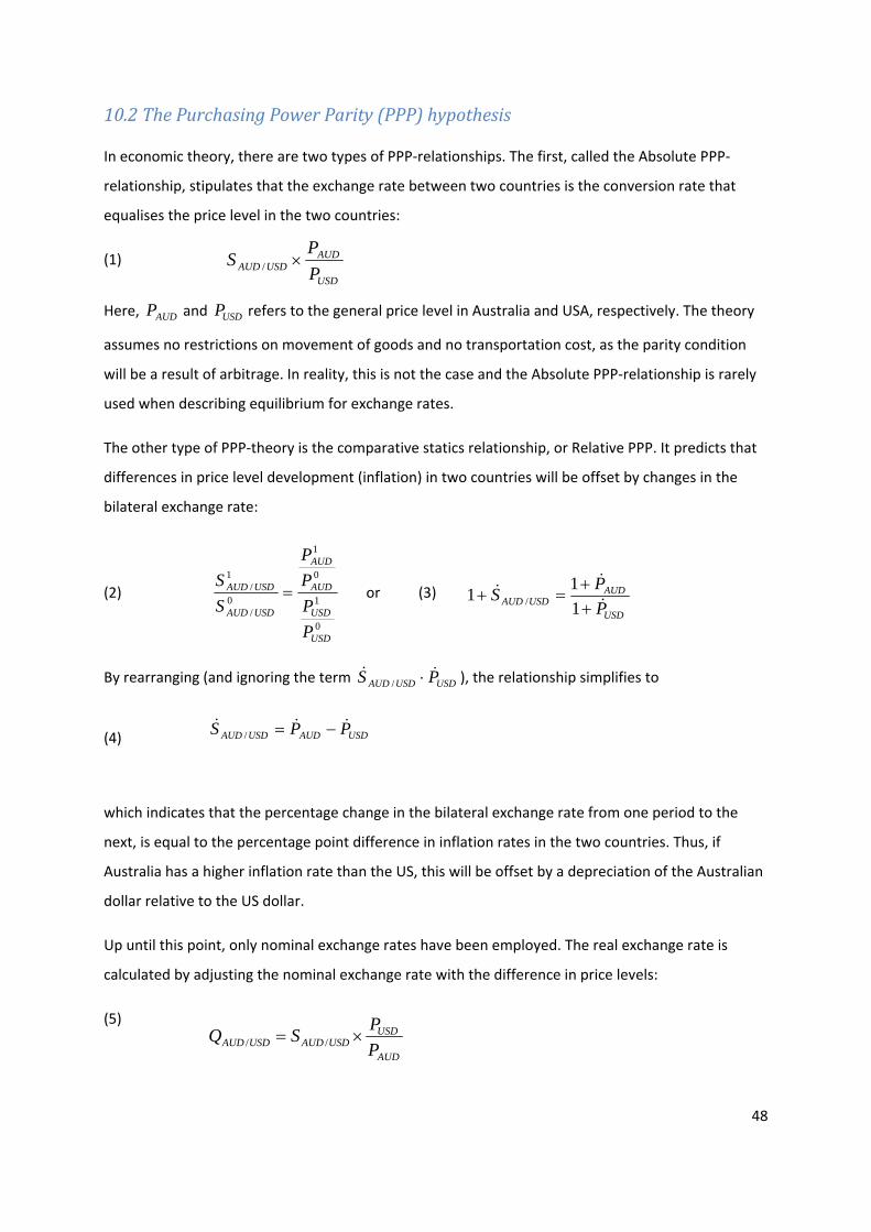
48
10.2 The Purchasing Power Parity (PPP) hypothesis
In economic theory, there are two types of PPP‐relationships. The first, called the Absolute PPP‐
relationship, stipulates that the exchange rate between two countries is the conversion rate that
equalises the price level in the two countries:
(1)
Here, AUDP and USDP refers to the general price level in Australia and USA, respectively. The theory
assumes no restrictions on movement of goods and no transportation cost, as the parity condition
will be a result of arbitrage. In reality, this is not the case and the Absolute PPP‐relationship is rarely
used when describing equilibrium for exchange rates.
The other type of PPP‐theory is the comparative statics relationship, or Relative PPP. It predicts that
differences in price level development (inflation) in two countries will be offset by changes in the
bilateral exchange rate:
(2)
0
1
0
1
0/
1/
USD
USD
AUD
AUD
USDAUD
USDAUD
PPPP
SS
= or (3)
By rearranging (and ignoring the term USDUSDAUD PS ⋅/ ), the relationship simplifies to
(4) USDAUDUSDAUD PPS −=/
which indicates that the percentage change in the bilateral exchange rate from one period to the
next, is equal to the percentage point difference in inflation rates in the two countries. Thus, if
Australia has a higher inflation rate than the US, this will be offset by a depreciation of the Australian
dollar relative to the US dollar.
Up until this point, only nominal exchange rates have been employed. The real exchange rate is
calculated by adjusting the nominal exchange rate with the difference in price levels:
(5)
USD
AUDUSDAUD P
PS++
=+111 /
AUD
USDUSDAUDUSDAUD P
PSQ ×= //
USD
AUDUSDAUD P
PS ×/
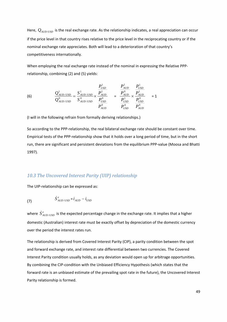
49
Here, USDAUDQ / is the real exchange rate. As the relationship indicates, a real appreciation can occur
if the price level in that country rises relative to the price level in the reciprocating country or if the
nominal exchange rate appreciates. Both will lead to a deterioration of that country’s
competitiveness internationally.
When employing the real exchange rate instead of the nominal in expressing the Relative PPP‐
relationship, combining (2) and (5) yields:
(6)
0
0
1
1
0/
1/
0/
1/
AUD
USD
AUD
USD
USDAUD
USDAUD
USDAUD
USDAUD
PPPP
SS
×= =
0
1
0
1
USD
USD
AUD
AUD
PPPP
0
0
1
1
AUD
USD
AUD
USD
PPPP
× = 1
(I will in the following refrain from formally deriving relationships.)
So according to the PPP‐relationship, the real bilateral exchange rate should be constant over time.
Empirical tests of the PPP‐relationship show that it holds over a long period of time, but in the short
run, there are significant and persistent deviations from the equilibrium PPP‐value (Moosa and Bhatti
1997).
10.3 The Uncovered Interest Parity (UIP) relationship
The UIP‐relationship can be expressed as:
(7) e
USDAUDS / = USDAUD ii −
where eUSDAUDS / is the expected percentage change in the exchange rate. It implies that a higher
domestic (Australian) interest rate must be exactly offset by depreciation of the domestic currency
over the period the interest rates run.
The relationship is derived from Covered Interest Parity (CIP), a parity condition between the spot
and forward exchange rate, and interest rate differential between two currencies. The Covered
Interest Parity condition usually holds, as any deviation would open up for arbitrage opportunities.
By combining the CIP‐condition with the Unbiased Efficiency Hypothesis (which states that the
forward rate is an unbiased estimate of the prevailing spot rate in the future), the Uncovered Interest
Parity relationship is formed.
50
Any deviations from the CIP‐condition will open for arbitrage opportunities, where market
participants profit from price discrepancies with no risk. Violation of the UIP‐condition on the other
hand, is based on investors’ belief that the forward rate is a biased estimate of the future spot rate.
Since trying to profit from such a violation requires transactions (long and short) separate in time,
there is exchange rate risk and a UIP‐position is classified as speculation.
A popular term for UIP‐speculation is carry trade. Carry traders believe that the UIP‐condition will not
hold and take a short position in one currency and a long position in another. Historically, carry trade
positions with funding in Japanese yen and investment in Australian or New Zealand dollars have
been profitable for carry traders. King (1998) found that the UIP‐condition held between Australia
and New Zealand after the removal of capital controls in the 1980s. This indicates that the two
markets became highly integrated following the deregulation.
The validity of the UIP‐condition has been analyzed extensively. Isard (1995) argues that it cannot be
tested in isolation since expectations about future exchange rates are unobservable and estimates of
such are of questionable quality. But under the assumption, the interest rate differential will be an
unbiased predictor of future exchange rate changes. Meese (1986) and Hodrick (1987) both found
strong evidence against the hypothesis of unbiasedness. Further analyses, such as Frenkel (1981) and
Mussa (1979) have concluded that the interest rate differential may affect the exchange rate, but its
effect is small.
10.4 The Real Interest Parity (RIP) relationship – The Fisher Equation
The final piece of theoretical foundation worth mentioning is linked to the other relationships.
Already mapped out is how a higher inflation rate erodes a nation’s competitiveness and thus leads
to nominal exchange rate depreciation (PPP), and how a higher interest rate must be offset by
expected depreciation of the nation’s currency (UIP). Why the higher interest rate yields this
outcome, will now be specified.
The Real Interest Parity (RIP) hypothesis is based on the assumption of highly integrated financial
markets. Thus, real interest rates on perfect substitutes of financial assets must be equal regardless
of the currency denomination.
The real interest rate is given by the equation:
51
(8) Pir
++
=+111
where r is the real interest rate, i is the nominal interest rate and P is the inflation rate. Since the
inflation rate is not known in advance, the expected inflation rate must be employed when
calculating the ex ante real interest rate. The Fisher equation is derived by substituting P with the
expected inflation rate eP and simplifying the equation above ( ePr ⋅ is very small):
(9) Fisher Equation: ee Pir −=
The relationship works perfectly if the nominal interest rate changes in proportion to the inflation
rate. The equation also explains why the Uncovered Interest Parity will hold in theory: Changes in a
nation’s nominal interest rate signals a change in expected inflation rate. By itself, the RIP condition
does little to discourage foreign investors from investing in high‐yielding, high‐inflationary markets. If
it did not affect the foreign exchange rate, the investors would merely convert the proceeds and not
be affected by the high inflation rate.
By combining the UIP and PPP relationship, the generalisation of the RIP‐condition is obtained:
(10) UIP: e
USDAUDS / = USDAUD ii −
(11) PPP: USDe
AUDe
USDAUDe PPS −=/
By rearranging them, this relationship follows:
(12) RIP: e
USDUSDe
AUDAUD PiPi −=−
Hence, if the two other parity conditions hold, it naturally follows that real interest rates must be
equal across currencies.
52
10.5 The relationship between the Australian dollar and Terms of Trade. An overview of previous analyses.
The Australian dollar has been labelled a “commodity currency”, primarily due to the country’s
reliance on commodity exports. This has some implications for the behaviour of the exchange rate,
most notably the variables of influence.
The rationale behind calling the Australian dollar a “commodity currency” is straightforward: As the
country’s exports consist of over 60 % commodities, the world price of commodities affects the
economy in a number of ways. The way commodity prices theoretically feed through to the exchange
rate can briefly be explained as follows:
In a situation where commodity prices increase, the Australian Terms of Trade will improve as prices
of exports increase while import prices remain unchanged. This will boost the nation’s income from
exports, improving its Balance of Payments (the Current Account surplus increase). The trade surplus,
reflecting foreigners’ demand for Australian goods, must be paid and therefore the trade
transactions increase the demand for Australian dollars. An increased demand for Australian dollars
yields the same result as for any other asset: The price goes up; the Australian dollar appreciates.
If reality replicated this theory, any change in commodity prices would take months before affecting
the value of the Australian dollar. In reality, participants in financial markets (those with investments
or debt expressed in Australian dollars) will find it beneficial to keep track of conditions in the foreign
exchange market. A number of financial indicators will give signals regarding potential direction of
the Australian dollar. Those participants, being rational and knowing that the Australian dollar is a
commodity currency, will therefore respond quickly to any unforeseen news about commodity price
developments.
10.5.1 Results of previous studies
There exists a rich selection of empirical studies examining the relationship between the Australian
dollar and Terms of Trade. The majority of these papers identify a robust long run‐relationship
between the two variables. Gruen and Wilkinson (1994) find only weak evidence of a stable, long‐
long run relationship, although their conclusion highlights the possibility of unidentified variables
obscuring the result of the analysis. Another possible explanation is the choice of data series;
53
quarterly data from 1969 to 1990. The Australian dollar was not floated until 1983, and hence a
robust relationship up until this point is less likely.
Karfakis and Phipps (1999) address the latter problem by employing a data series of monthly
observations from January 1984 to December 1995. By analyzing the nominal USD/AUD exchange
rate and the Australian Terms of Trade over the period, they find the long‐run relationship
ln(USD/AUD) = ‐4.50 + 0.93 ln(Terms of Trade)
Hence, their result suggests a relationship close to unity between the two variables.
The implication of these results is that the real Australian dollar may not have a long‐run equilibrium
value as suggested by the Purchasing Power Parity theory. The currency’s reliance on world
commodity prices is indicated to be strong, and commodity prices are themselves the result of global
supply and demand rather than an equilibrium value dictated by fundamentals. For many other
currencies, the Purchasing Power Parity theory holds over the long term, where fluctuations around
the parity‐value are temporary. It is more unclear whether this long‐run equilibrium exists for the
real Australian dollar.
10.5.2 The limitations of Terms of Trade as an explanatory variable to exchange rate movements
Several studies have highlighted problems concerning the Terms of Trade as an explanatory variable
with respect to the exchange rate. In their analysis, Chen and Rogoff (2003) discuss the limitations of
employing this measure as an independent variable. When modelling the exchange rate, the
independent variables are assumed exogenously determined. In reality, there might be a two‐way
causality between the exchange rate and the Terms of Trade, resulting in biased estimates.
There are two main reasons why Terms of Trade might be affected by the exchange rate. Terms of
Trade is the ratio of export prices to import prices. Under the assumption of Terms of Trade being
exogenously determined, any change in the exchange rate will alter the domestic prices of exports
and imports by the same ratio, leaving the Terms of Trade unchanged. But if exchange rate pass‐
through to the domestic market is incomplete, in the sense that pricing to market does not fully
reflect changes in the exchange rate, the ratio of export prices‐to‐import prices will be altered. In this
case, there will be a feedback effect from the exchange rate to the Terms of Trade.
54
Another reason why Terms of Trade might not satisfy the assumption of strict exogenity, is if the
country in question is a dominant supplier in the export market. If the country is not a price taker in
the market, changes in the exchange rate will lead to changes in export prices but not import prices.
This will also yield a feedback effect from the value of the domestic currency to Terms of Trade.
Karfakis and Phipps (1999) found little evidence of causality running from the Australian exchange
rate to the Terms of Trade. In other words, Australia appears to be a price taker in the export market.
Even though Australia is a leading world exporter of commodities such as wool and coal, the
presence of substitute commodities is likely to weaken its power in these markets. Chen and Rogoff
(2003) omitted the problems associated with Terms of Trade as an independent variable by
employing a country‐specific index of world commodity prices. Acknowledging that the variable
might still be affected by a country’s pricing power in export markets, they also analyzed the
relationship between the exchange rate and a broader world commodity price index. For both types
of commodity price indices, a robust relationship with the Australian dollar was found.
Besides from the endogeniety problem, there exists another compelling reason to substitute Terms
of Trade with a commodity price index when modelling the Australian exchange rate. Terms of Trade
is reported quarterly by the Australian Bureau of Statistics. Given that the exchange rate responds
quickly to commodity price changes, it cannot be caused by Terms of Trade. Therefore, it is rational
to assume that this ex‐post figure has little practical relevance for participants in financial markets.
Although it is highly correlated with commodity prices, the infrequent and lagged publication makes
it unlikely to be the cause of financial transactions involving the Australian dollar. Commodity prices
are quoted every day and this measure is more likely to affect the behaviour of international traders.
Due to this, Hatzinikolaou and Polasek (2005) use commodity price level as an explanatory variable in
their model of the Australian dollar.
In the next chapter, the model variables will be presented. The choice of variables is based on the
parity relationships and empirical evidence addressed in this chapter.
55
CHAPTER 11. THE MODEL VARIABLES
The thesis explicitly states that the period of interest is the recent financial crisis spanning from mid
2007 to end 2009. Analyzing its effect on the Australian currency requires the model to be tailored to
this specification. To best capture the dynamics of the foreign exchange market, monthly
observations is a rational choice of data frequency. Daily observations would provide a larger sample,
but day‐to‐day fluctuations are difficult to explain by economic fundamentals reported less
frequently. Monthly figures provide a smoother set of observations. In order for the sample size to
be sufficiently large, the period January 2005 to December 2009 is analyzed.
11.1 The dependent variable: Nominal exchange rate, “TWI/AUD”
The nominal exchange rate between the Australian dollar and the Trade Weighted Index will be the
dependent variable in the model. The monthly average has been calculated from daily values13
retrieved from the Reserve Bank of Australia’s webpage. The exchange rate is expressed in indirect
form, as the TWI‐value of one Australian dollar. This is for pedagogical purposes – a lower exchange
rate signals depreciation, and vice versa.
When deciding upon an appropriate dependent variable, there are several factors to take into
account. Based on the aim of this thesis, the development of the Australian dollar should be
expressed relative to a broad currency index like TWI. Considering how the United States is not an
appropriate economy to represent the general global trend during the last 5 years, the Trade
Weighted Index yields more insight regarding the general condition of the Australian dollar.
The effective exchange rate TWI/AUD has some limitations. The Index is based on the nominal
bilateral exchange rates of the Australian dollar against 22 other currencies. Finding consumer price
indices for all these countries is a near impossible task, both regarding access and quality of data.
Therefore, the exchange rate must be expressed in nominal terms. Due to this, the independent
variables in the model are also expressed in nominal figures.
In the following, the model’s independent variables are presented. Whenever a variable is the
differential between the Australian and foreign value of a financial indicator, the proxy for the
outside world is the average of domestic figures for USA, UK, Germany and Japan. The development
13 The daily value is the exchange rate measured at 4.00 pm (Australian time).
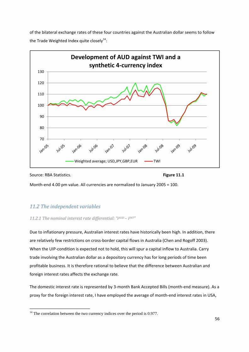
56
of the bilateral exchange rates of these four countries against the Australian dollar seems to follow
the Trade Weighted Index quite closely14:
Source: RBA Statistics. Figure 11.1
Month‐end 4.00 pm value. All currencies are normalized to January 2005 = 100.
11.2 The independent variables
11.2.1 The nominal interest rate differential: “iAUD – iINT”
Due to inflationary pressure, Australian interest rates have historically been high. In addition, there
are relatively few restrictions on cross‐border capital flows in Australia (Chen and Rogoff 2003).
When the UIP‐condition is expected not to hold, this will spur a capital inflow to Australia. Carry
trade involving the Australian dollar as a depository currency has for long periods of time been
profitable business. It is therefore rational to believe that the difference between Australian and
foreign interest rates affects the exchange rate.
The domestic interest rate is represented by 3‐month Bank Accepted Bills (month‐end measure). As a
proxy for the foreign interest rate, I have employed the average of month‐end interest rates in USA,
14 The correlation between the two currency indices over the period is 0.977.
70
80
90
100
110
120
130
Development of AUD against TWI and a synthetic 4‐currency index
Weighted average; USD,JPY,GBP,EUR TWI
57
UK, Germany and Japan. For USA, the interest rate employed is the secondary market yield of 3‐
month Treasury bills. For UK, 3‐month Treasury bills (middle rate, tender) are used. For Japan and
Germany, I have employed the 3‐month Interbank offer rates due to the unavailability of 3‐month
Government bill yields. Ideally, all interest rates would be of comparable money market instruments,
reflecting the relatively risk‐free rate on deposits. Nevertheless, money market spreads in USA and
UK have been significantly higher than in the other three countries15. Therefore, I have deemed the
interest rates employed as the most comparable set. All the interest rates have been retrieved from
Thomson Reuters Datastream.
The nominal interest rate differential is expressed in per cent as
Since the interest rates are measured at month‐end, and represent money market yields over the 3
months following, it would not be meaningful to estimate the impact on the exchange rate in the
prevailing month. Therefore, the variable is included in the model with a one, two and three month
lag.
11.2.2 The inflation differential: “pAUD – pINT”
In line with the PPP condition, a proxy for inflation differential between Australia and foreign
economies is included as an independent variable in the model. For Australia, only quarterly figures
are available (and retrieved from RBA’s home page). This poses a problem, since all other variables in
the model are stated in monthly terms. One solution would be to set the price level equal for the
three months in each quarter. However, the issue has been resolved by using linear interpolation on
the missing observations.
As a representation of development in the foreign price level, Consumer Price indices for USA, UK,
Germany and Japan were retrieved from Thomson Reuters Datastream. These indices are all
reported in monthly terms. By normalising the indices to November 2004 = 100 and calculating the
simple average, an index representing price development outside Australia is constructed.
15 For details, please see section 2.2.
58
The difference between Australian and foreign inflation is then expressed as
where small letters represent the value in logarithmic form.
November 2004 as the base period is not a random choice. Firstly, since the Australian CPI index is
stated quarterly, the base period must be a month where CPI is reported in order for the linear
interpolation approximation to be consistent with the quarterly reported figures. Secondly, since
both the Australian and the foreign CPI indices are normalised to 100 the same month (for
consistency) inflation differential in the base month will be zero. Third of all, it is not clear prior to
the empirical analysis whether inflation will affect the exchange rate immediately. In which case, it
would imply that market participants expect the prevailing inflation rate that is reported ex‐post.
This might be an unreasonable assumption, and a solution would be to assume that inflation
expectations are adaptive. Blinder (1988) and Ball (1991) both regard this to be the most reasonable
assumption. In this case, the inflation rate differential variable should be employed with a one month
lag.
11.2.3 Commodity Price index: “CCI”
The commodity price index of choice is the Thomson Reuters Equal Weight Continuous Commodity
Index. It is a broad commodity index, comprising of 17 continuously rebalanced commodity futures.
CCI is calculated from the USD‐price of futures contracts on these commodities, and therefore
captures the broad movements in world commodity prices. The CCI‐index was retrieved from
Thomson Reuters Datastream. Daily observations are employed to calculate the monthly average.
When including the CCI‐index as an independent variable in the model, it is assumed that the US
dollar exchange rate does not affect the quoted prices. Assuming that the index value is strictly
exogenously determined by global supply and demand is a simplification, but the assumption is
common to make in econometric analyses.
11.2.4 Volatility in the Australian dollar: “Vol”
This percentage point measure is derived from prices of three‐month options on Australian dollars,
and the volatility time series was retrieved from Thomson Reuters Datastream. This variable
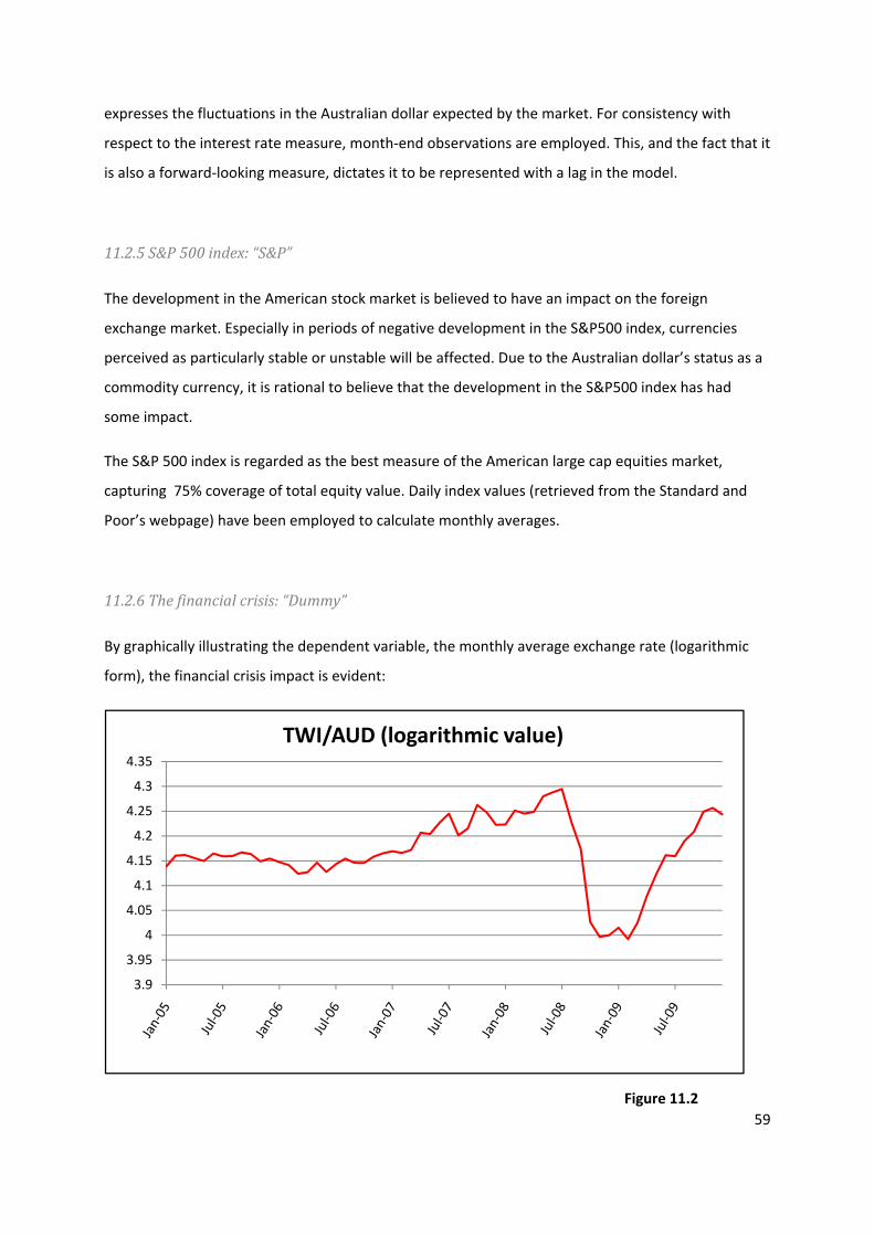
59
expresses the fluctuations in the Australian dollar expected by the market. For consistency with
respect to the interest rate measure, month‐end observations are employed. This, and the fact that it
is also a forward‐looking measure, dictates it to be represented with a lag in the model.
11.2.5 S&P 500 index: “S&P”
The development in the American stock market is believed to have an impact on the foreign
exchange market. Especially in periods of negative development in the S&P500 index, currencies
perceived as particularly stable or unstable will be affected. Due to the Australian dollar’s status as a
commodity currency, it is rational to believe that the development in the S&P500 index has had
some impact.
The S&P 500 index is regarded as the best measure of the American large cap equities market,
capturing 75% coverage of total equity value. Daily index values (retrieved from the Standard and
Poor’s webpage) have been employed to calculate monthly averages.
11.2.6 The financial crisis: “Dummy”
By graphically illustrating the dependent variable, the monthly average exchange rate (logarithmic
form), the financial crisis impact is evident:
Figure 11.2
3.9
3.95
4
4.05
4.1
4.15
4.2
4.25
4.3
4.35
TWI/AUD (logarithmic value)
60
The last observation before the large drop (depreciation) is June 2008. This indicates that a dummy
variable representing the financial crisis should be included, with a value of 0 up until June 2008 and
the value 1 for the remaining observations in the sample. The dummy is then multiplied with the
other independent variables to see where the financial crisis alters the effect the independent
variables have on the exchange rate.
When discussing the model, the period where the dummy variable is assigned a value of 1 (July 2008
– December 2009) is referred to as the financial crisis.
11.3 Final remarks
All variables except the interest rate and volatility (which are expressed in percent) are expressed in
logarithmic form. The rationale behind using logarithms instead of the variable’s original form is that
the OLS‐regression estimates a linear relationship between the variables. For many economic time
series, the trend is not linear but exponential (Wooldridge 2006). By converting the variables to
natural logarithms the trend becomes linear, expressing the growth rate.
I have deliberately omitted variables linking the exchange rate to indicators of real economic
development such as GDP growth and the Balance of Payments. The reason for this is twofold.
Firstly, real economic figures are primarily reported on a quarterly basis and would therefore have to
be lagged several months if included in the model. This would undermine the purpose of the model;
to identify which short‐term dynamic effects that have steered the development of the Australian
dollar. And secondly, there is no consensus on which real economic variables to include in an
exchange rate model. Economic variables react with different pace to external shocks. Mapping out
these variables is therefore beyond the scope of the thesis.
61
CHAPTER 12. TIME SERIES AND THEIR SUITABILITY FOR REGRESSION ANALYSIS16
12.1 Necessary characteristics
Time series data differ from data obtained by random sampling. Therefore, certain characteristics
should be present in the time series in order for it to be employed in a regression model.
One of these characteristics is stationarity. A strictly stationary time series is one where the
observations have a constant mean and variance across time, and the covariance between any two
observations is only dependent of their distance apart in time. Strict stationarity is a strong
assumption and puts restraints on the joint distribution of a time series across time. Furthermore,
the strict stationarity assumption is not required to hold in order for the time series to be employed
in a regression.
A weaker form of stationarity, where the variance is not necessarily constant but finite is on the
other hand a condition of requirement. This concept is formally referred to as covariance‐stationarity
(Sarno and Taylor 2006), and will in the following be called stationarity. If the time series is not
stationary, it will not yield meaningful information when included in a regression. The time series’
statistical characteristics must be stable across time to compensate for the fact that the observations
are not obtained by random sampling.
12.2 Dickey Fuller test for stationarity
One way of testing if a time series is stationary is with the Dickey Fuller test. By expressing the time
series as an autoregressive process of order one, AR(1):
(13) , 1,2, …
It can be shown that if | |< 1, the time series is stationary and is called an I(0)‐process. In the other
case, where = 1, it has a unit root, and is called an I(1)‐process.
Modifying the expression above will make it suitable for testing whether the process has a unit root.
Some variables are trend‐stationary, where the mean is linearly dependent on time, but the process
16 Unless otherwise stated, this chapter is based on Wooldridge (2006).
62
is stationary about its trend. This is an I(0)‐process but can be mistaken for an I(1)‐process if a trend
variable is not included. By subtracting from both sides of equation (13) and including a trend
component, the regression equation is now
(14) ∆ 1
The null hypothesis is : 1 0
Against : 1 0
Under , has a unit root which implies that the asymptotic standard normal distribution for
the t‐statistic is invalid. This is due to the theoretically infinite variance (Sarno and Taylor 2006). The
name of the test stems from the Dickey Fuller distribution tabulating the critical rejection values of
the t‐statistic for the test. There are different critical rejection values for a test with and without a
trend component.
If the null hypothesis is rejected, the time series is regarded as stationary, hence an I(0)‐process. If it
cannot be rejected, we do not state that the time series positively have a unit root. We simply
conclude that there is not enough statistical evidence to reject the unit root hypothesis, and must
therefore be careful to use the time series in its original form in a regression model.
If the null hypothesis is not rejected, it can be proven that the first difference of a unit root‐process is
stationary. Therefore, time series with an I(1)‐process must be differentiated before employed in a
regression analysis.
12.3 Augmented Dickey Fuller test
Since the Dickey Fuller Test in its original form (14) does not account for serial correlation in ∆ , an
Augmented Dickey Fuller test including lags is more appropriate. The modification of the original test
can be algebraically stated as
(15) ∆ 1 ∑ ∆
63
Where n represents number of lags included. By including lags, the power of the test is reduced since
observations are lost. But not including lags will yield an incorrect size of the test, since the validity of
the critical t‐values is dependent on the dynamics being completely modelled. The t‐statistics for the
lagged changes have approximately t‐distributions. This will be indicative of whether enough lags
have been included in the Augmented Dickey Fuller test.
12.4 Cointegration
Even if variables follow an I(1)‐process, they can be included in a regression model in their original
form if they are cointegrated with other variables in the model. The intuition follows from the fact
that two independent I(1)‐processes (x and y) combined also will be an I(1)‐process:
(16)
This linear combination will yield error terms, which also have a unit root. But if the two variables
are cointegrated, their non‐stationary characteristics will cancel each other out and the error term
will be stationary. Therefore, testing for cointegration is conducted by testing if a linear combination
of two variables is stationary, as will be revealed by the error terms of the relationship.
Testing for cointegration is conducted in a similar manner as with the stationarity test. First,
regressing two unit root variables against each other yields the residuals:
(17) ̂
These residuals can be tested with the Augmented Dickey Fuller method previously explained
(equation (15), without trend component). Since the Ordinary Least Squares regression technique
minimizes the sum of squared residuals, they might appear to be an I(0) process even if x and y are
not cointegrated. Therefore, the critical value for the t‐ statistic is of an even larger magnitude than
for the regular Dickey Fuller test.
The identification of cointegration between variables is central in econometrics, as it reveals a stable
long‐run relationship. The linear combination of the cointegrating variables is stationary – which
implies that they fluctuate around an equilibrium value. Cointegrating relationships convey
important information about how economic variables relate to one another. However, the focus of
this thesis is on revealing short‐run dynamics in the Australian exchange rate. Any long‐run
relationships are unlikely to dictate the exchange rate in the rather turbulent period of interest.
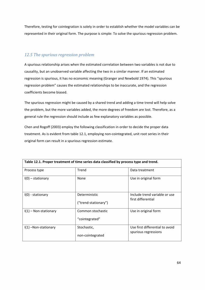
64
Therefore, testing for cointegration is solely in order to establish whether the model variables can be
represented in their original form. The purpose is simple: To solve the spurious regression problem.
12.5 The spurious regression problem
A spurious relationship arises when the estimated correlation between two variables is not due to
causality, but an unobserved variable affecting the two in a similar manner. If an estimated
regression is spurious, it has no economic meaning (Granger and Newbold 1974). This “spurious
regression problem” causes the estimated relationships to be inaccurate, and the regression
coefficients become biased.
The spurious regression might be caused by a shared trend and adding a time trend will help solve
the problem, but the more variables added, the more degrees of freedom are lost. Therefore, as a
general rule the regression should include as few explanatory variables as possible.
Chen and Rogoff (2003) employ the following classification in order to decide the proper data
treatment. As is evident from table 12.1, employing non‐cointegrated, unit root series in their
original form can result in a spurious regression estimate.
Table 12.1. Proper treatment of time series data classified by process type and trend.
Process type Trend Data treatment
I(0) – stationary
None Use in original form
I(0) ‐ stationary Deterministic
(“trend‐stationary”)
Include trend variable or use first differential
I(1) – Non‐stationary Common stochastic
“cointegrated”
Use in original form
I(1) –Non‐stationary Stochastic,
non‐cointegrated
Use first differential to avoid spurious regressions
65
12.6 Interpretation of a regression estimate
12.6.1 The R2 and R2adjusted estimate
The R2‐estimate expresses how much of the total variance in the dependent variable is captured by
the regression model. It is the model’s explanatory power, or the fraction of the sample variation in
the dependent variable that is explained by the independent variables. The value is calculated by
dividing the Explained Sum of Squares (SSE) by the Total Sum of Squares (SST). The remaining
(unexplained) portion of total variance is the Sum of Squared Residuals (SSR) – which is the measure
the OLS‐regression estimate minimizes – divided by SST. Squaring the residuals is done in order for
positive and negative residuals not to cancel each other out, and to penalize large deviations more
severely than small ones.
The R2‐adjusted prevails when adjusting the R2 by the number of independent variables in the
regression estimate. It is a better measure of the explanatory power of a model, since adding
another independent variable will not cause the R2 to decrease, but it will cost one degree of
freedom.
12.6.2 The Root Mean Square Error (RMSE) estimate
This measure is another output of a regression analysis, and indicates the standard deviation in the
residuals. Small variance (standard deviation) in the residuals is desirable.
12.6.3 The DurbinWatson Statistic
The Durbin‐Watson statistic is also based on the OLS‐residuals. It indicates if there is a problem with
serial correlation in the residuals, which would imply that a variable has been omitted in the
regression. The Durbin‐Watson statistic is close to 2 when no serial correlation is present. Savin and
White (1977) has created a table for upper‐ and lower bound critical values. Depending on number
of observations and independent variables, one can test for serial correlation in the residuals. If the
reported Durbin Watson‐statistic falls below the lower bound, serial correlation is present. If the DW‐
statistic is above the upper bound, the null hypothesis of no serial correlation cannot be rejected. If
the DW‐statistic falls between the lower and upper bound, the test is inconclusive.
66
12.6.4 Coefficient pvalues
For each independent variable, a p‐value is reported. It indicates at which level the hypothesis of the
coefficient being significantly different from zero can be rejected. Generally, one wishes to reject this
hypothesis at a 5 % level of significance. Therefore, variables where the p‐value of the coefficient is
larger than 0.05 should be removed from the regression estimate, as it indicates that the estimated
coefficient might be 0 – hence, the variable is not explanatory with respect to the dependent
variable.
12.6.5 The Standard Error (SE) of the Coefficients
For each independent variable, Minitab reports the respective standard error of the estimated
coefficient. This is an indication of how precise the estimated coefficient is. It is desirable to have
small Standard Errors of the coefficients. If one wishes to construct a 95 % confidence interval for the
value of a coefficient, a large estimated Standard Error will cause the interval to be very wide. Even
though the coefficient value is an unbiased estimate, it contains a level of uncertainty that reduces
the informational value of the model.
12.6.6 The Variance Inflation Factor
One problem that can arise in regression analysis is multicollinearity. This occurs if some of the
independent variables included are highly correlated. Multicollinearity is a problem because it
creates very high variance in the least squares estimates and makes the regressed coefficients of the
independent variables very imprecise. Also, the Standard Error (SE) of the coefficients will be very
high, or ‘inflated’ (Mendenhall and Sincich 2003).
For each independent variable, Minitab reports a Variance Inflation Factor (VIF)17. As a rule of
thumb, the Variance Inflation Factor should be less than 10. If the VIF‐value is higher than 10, it
indicates multicollinearity. There exist several statistical techniques to deal with multicollinearity.
Nevertheless, the easiest way is to remove the variable(s) displaying high degree of correlation to
others, as they do not contain much additional information.
17 Please see Appendix A for an explanation of the Variance Inflation Factor
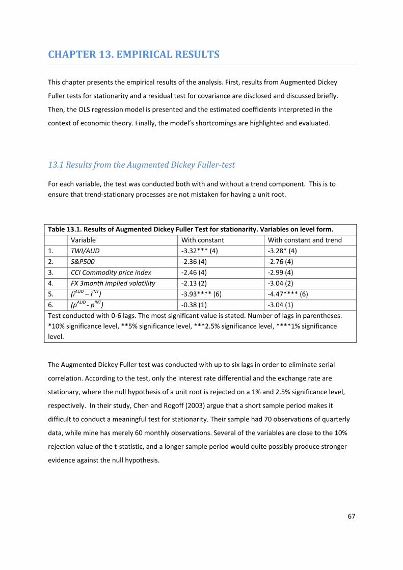
67
CHAPTER 13. EMPIRICAL RESULTS
This chapter presents the empirical results of the analysis. First, results from Augmented Dickey
Fuller tests for stationarity and a residual test for covariance are disclosed and discussed briefly.
Then, the OLS regression model is presented and the estimated coefficients interpreted in the
context of economic theory. Finally, the model’s shortcomings are highlighted and evaluated.
13.1 Results from the Augmented Dickey Fullertest
For each variable, the test was conducted both with and without a trend component. This is to ensure that trend‐stationary processes are not mistaken for having a unit root.
Table 13.1. Results of Augmented Dickey Fuller Test for stationarity. Variables on level form.
Variable With constant With constant and trend
1. TWI/AUD ‐3.32*** (4) ‐3.28* (4)
2. S&P500 ‐2.36 (4) ‐2.76 (4)
3. CCI Commodity price index ‐2.46 (4) ‐2.99 (4)
4. FX 3month implied volatility ‐2.13 (2) ‐3.04 (2)
5. (iAUD – iINT) ‐3.93**** (6) ‐4.47**** (6)
6. (pAUD ‐ pINT) ‐0.38 (1) ‐3.04 (1)
Test conducted with 0‐6 lags. The most significant value is stated. Number of lags in parentheses. *10% significance level, **5% significance level, ***2.5% significance level, ****1% significance level.
The Augmented Dickey Fuller test was conducted with up to six lags in order to eliminate serial
correlation. According to the test, only the interest rate differential and the exchange rate are
stationary, where the null hypothesis of a unit root is rejected on a 1% and 2.5% significance level,
respectively. In their study, Chen and Rogoff (2003) argue that a short sample period makes it
difficult to conduct a meaningful test for stationarity. Their sample had 70 observations of quarterly
data, while mine has merely 60 monthly observations. Several of the variables are close to the 10%
rejection value of the t‐statistic, and a longer sample period would quite possibly produce stronger
evidence against the null hypothesis.
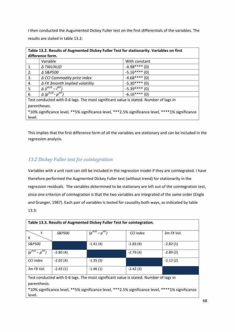
68
I then conducted the Augumented Dickey Fuller test on the first differentials of the variables. The
results are stated in table 13.2:
Table 13.2. Results of Augmented Dickey Fuller Test for stationarity. Variables on first difference form. Variable With constant 1. ∆ TWI/AUD ‐4.98**** (0) 2. ∆ S&P500 ‐5.16**** (0) 3. ∆ CCI Commodity price index ‐4.68**** (0) 4. ∆ FX 3month implied volatility ‐5.30**** (0) 5. ∆ (iAUD – iINT) ‐5.39**** (0) 6. ∆ (pAUD ‐ pINT) ‐6.16**** (0) Test conducted with 0‐6 lags. The most significant value is stated. Number of lags in parentheses. *10% significance level, **5% significance level, ***2.5% significance level, ****1% significance level.
This implies that the first difference form of all the variables are stationary and can be included in the regression analysis.
13.2 Dickey Fuller test for cointegration
Variables with a unit root can still be included in the regression model if they are cointegrated. I have
therefore performed the Augmented Dickey Fuller test (without trend) for stationarity in the
regression residuals. The variables determined to be stationary are left out of the cointegration test,
since one criterion of cointegration is that the two variables are integrated of the same order (Engle
and Granger, 1987). Each pair of variables is tested for causality both ways, as indicated by table
13.3:
Table 13.3. Results of Augmented Dickey Fuller Test for cointegration.
Y X
S&P500 (pAUD – pINT) CCI index 3m FX Vol.
S&P500 ‐1.41 (4) ‐1.83 (4) ‐2.82 (1)
(pAUD – pINT) ‐2.80 (4) ‐2.79 (4) ‐2.89 (2)
CCI index ‐2.02 (4) ‐1.35 (3) ‐2.12 (2)
3m FX Vol. ‐2.43 (1) ‐1.46 (1) ‐2.42 (3)
Test conducted with 0‐6 lags. The most significant value is stated. Number of lags in parenthesis. *10% significance level, **5% significance level, ***2.5% significance level, ****1% significance level.
69
As stated in the previous chapter, the residuals of an OLS‐ regression tend to replicate an I(0)‐
process. Therefore, the critical values for the t‐statistic are high and none of the t‐values in the table
are even close to the critical values. Therefore, no cointegrating relationships have been identified.
Chen and Rogoff (2003) had 70 observations of quarterly data in their sample, and their opinion was
that cointegration tests have little statistical power in such short time series. I therefore have to
conclude that there might be cointegrating relationships between the variables of interest, but my
number of observations and sample period precludes informative test results.
The Dickey Fuller cointegration test on residuals has been criticized for rejecting the null hypothesis
of no cointegration too often (Kremers et al. 1992). This problem is linked to the residuals imitating
an I(0)‐process even when x and y are not cointegrated. However, this critique is irrelevant to the
test results, since the null hypothesis was not rejected for any of the variable pairs. Employing a more
stringent technique of testing is unlikely to shed more light on my lack of affirmative results.
13.3 Implications of the tests
The t‐statistic for the inflation differential is very close to the 10% critical rejection value for the
Augmented Dickey Fuller test with trend. Conducting an OLS‐regression on the variable (pAUD – pINT)
provided some insight. The regression line is estimated to be:
(18) (pAUD – pINT) = 0.000535 + 0.000994*trend
The R2‐adjusted for this fitted line is 96.5%, describing how much of the total variance in the time
series is explained by the regression estimate. It seems like there is a very prominent trend in the
inflation differential data:
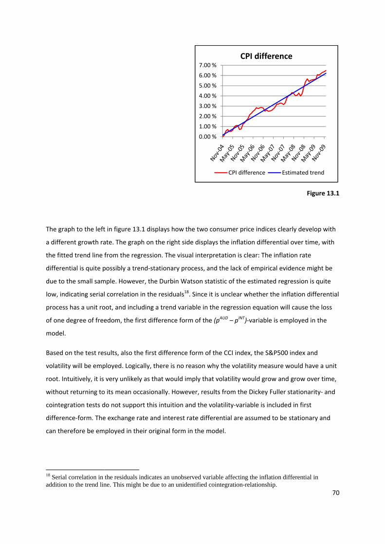
The grap
a differe
the fitte
different
due to th
low, indi
process
of one d
model.
Based on
volatility
root. Int
without
cointegr
differenc
can ther
18 Serial caddition t
ph to the left
ent growth ra
d trend line
tial is quite p
he small sam
icating serial
has a unit ro
egree of free
n the test res
y will be emp
uitively, it is
returning to
ration tests d
ce‐form. The
refore be em
correlation in to the trend lin
t in figure 13
ate. The grap
from the reg
possibly a tre
mple. Howeve
l correlation
oot, and inclu
edom, the fi
sults, also th
ployed. Logic
very unlikely
o its mean oc
do not suppo
e exchange r
mployed in th
the residuals ine. This migh
3.1 displays h
ph on the rig
gression. The
end‐stationa
er, the Durb
in the residu
uding a trend
rst differenc
he first differ
cally, there is
y as that wo
ccasionally. H
ort this intuit
ate and inte
eir original f
indicates an ut be due to an
how the two
ht side displ
e visual inter
ry process, a
in Watson st
uals18. Since
d variable in
e form of th
ence form o
s no reason w
uld imply tha
However, res
tion and the
rest rate diff
form in the m
unobserved van unidentified
0.00
1.00
2.00
3.00
4.00
5.00
6.00
7.00
consumer p
ays the infla
rpretation is
and the lack o
tatistic of the
it is unclear
the regressi
e (pAUD – pINT
f the CCI ind
why the vola
at volatility w
sults from th
volatility‐var
ferential are
model.
riable affectincointegration-
0 %
0 %
0 %
0 %
0 %
0 %
0 %
0 %C
CPI dif
rice indices c
tion differen
clear: The in
of empirical
e estimated
whether the
on equationT)‐variable is
ex, the S&P5
tility measur
would grow a
e Dickey Ful
riable is inclu
assumed to
ng the inflation-relationship.
CPI differe
fference
Fig
clearly devel
ntial over tim
nflation rate
evidence mi
regression is
e inflation dif
will cause th
employed in
500 index an
re would hav
and grow ov
ler stationar
uded in first
be stationar
n differential
ence
Estimated tr
70
gure 13.1
lop with
me, with
ight be
s quite
fferential
he loss
n the
nd
ve a unit
ver time,
rity‐ and
ry and
in
rend
71
13.4 The OLS regression model
13.4.1 Introductory remarks
The process of constructing an OLS‐regression model began by including all the variables in the
regression equation. Also lagged versions of the variables were included. The exchange rate with a
one period lag was also included as an independent variable in order to remove serial correlation in
the residuals. By a stepwise reduction of variables included based on their respective p‐values, a first
draft of the model emerged.
The majority of independent variables were stated in first difference form. It quickly became
apparent that this “hybrid model” comprising of both original‐ and first difference‐form variables
suffered from several shortcomings. Firstly, the lagged exchange rate variable’s coefficient was
estimated to be 1.05, which is not significantly different from 1. Therefore, the dependent variable
(the exchange rate) can be expressed in first difference form. And secondly, the interest rate
differentials with a one‐ and three‐month lag were significant at a 5% level but suffered from high
degree of multicollinearity (which was evident from their VIF‐estimates). The mix of first difference
and original variables proved to be difficult to work with. Therefore, even though the interest rate
differential and the exchange rate were found to be stationary in section 13.1, the first difference
form of these is better to work with.
Engel (2000) argues that a stationary process can always be arbitrarily well approximated by a non‐
stationary process in finite samples (and vice versa). Therefore, the results from the stationarity test
in table 13.1 might be misleading and cause the regression estimate to be spurious. A pure
differential form model solves the aforementioned problems with the original form variables, as well
as ensuring that the estimates are not spurious.
13.4.2 The pure differential model
The function Best Subset in Minitab suggests different combinations of the independent variables
which yields a good fit for the regression model. For each combination‐set, the corresponding R2, R2‐
adjusted and RMSE‐value are also stated. The methodical process of obtaining the best fit for the
data is explained in Appendix B.
72
The following fitted model explained the data best (standard errors in parentheses):
(19) 3)(66.1271.0&168.000218.0/ −−Δ+Δ+Δ+−=Δ tINTAUD
ttt iiCCIPSAUDTWI
(0.001952) (0.04974) (0.0708) (0.8133)
21 )(84.4273.0275.0 −− −Δ∗−Δ∗+Δ− tINTAUD
tt iiDummyCCIDummyVol
(0.1332) (0.1016) (1.251)
112 )(0.149374.0 −−− −Δ∗Δ∗−Δ∗− tINTAUD
tt iiVolDummyVolDummy
(0.1536) (32.07)
R2 =84,5% R2‐adjusted = 82.1% RMSE = 0,0128294 DW = 2.03697
All the explanatory variables are significant at a 5% level. Both the R2‐adjusted and the RMSE‐value
indicate a good fit. Furthermore, the Durbin Watson statistic is above the critical upper‐bound value
for a sample with 59 observations and 9 independent variables (including the intercept)19, and the
null hypothesis of no serial correlation cannot be rejected at a 5 % level. Therefore, it is assumed to
be no serial correlation in the residuals.
The intercept has a p‐value of 0.27, which implies that the hypothesis of this value being significantly
different from 0 cannot be rejected at a 5% level. But even if the intercept is not statistically
significant at a 5% level, it is common in statistics to include it (Mendenhall and Sincich 2003).
Therefore, the intercept is kept.
19 The critical upper-bound value is 1.89665 (Savin and White 1977).
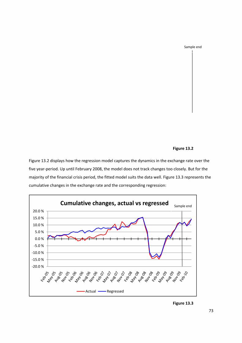
Figure 13
five year
majority
cumulat
‐20.0 %
‐15.0 %
‐10.0 %
‐5.0 %
0.0 %
5.0 %
10.0 %
15.0 %
20.0 %
3.2 displays
r‐period. Up
y of the finan
ive changes
%
%
%
%
%
%
%
%
%
Cu
how the reg
until Februa
ncial crisis pe
in the excha
umulativ
A
ression mod
ary 2008, the
eriod, the fitt
ange rate and
ve change
Actual Re
del captures t
e model does
ted model su
d the corresp
es, actua
egressed
the dynamic
s not track ch
uits the data
ponding regr
al vs regr
F
cs in the exch
hanges too c
well. Figure
ression:
F
ressed S
igure 13.2
hange rate ov
closely. But f
13.3 represe
igure 13.3
Sample e
Sample end
73
ver the
or the
ents the
end
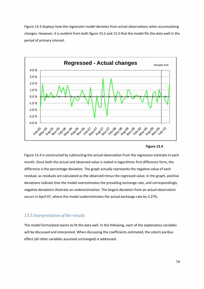
74
Figure 13.3 displays how the regression model deviates from actual observations when accumulating
changes. However, it is evident from both figure 13.2 and 13.3 that the model fits the data well in the
period of primary interest.
Figure 13.4
Figure 13.4 is constructed by subtracting the actual observation from the regression estimate in each
month. Since both the actual and observed value is stated in logarithmic first difference form, the
difference is the percentage deviation. The graph actually represents the negative value of each
residual, as residuals are calculated as the observed minus the regressed value. In the graph, positive
deviations indicate that the model overestimates the prevailing exchange rate, and correspondingly
negative deviations illustrate an underestimation. The largest deviation from an actual observation
occurs in April 07, where the model underestimates the actual exchange rate by 3.27%.
13.5 Interpretation of the results
The model formulated seems to fit the data well. In the following, each of the explanatory variables
will be discussed and interpreted. When discussing the coefficients estimated, the ceteris paribus
effect (all other variables assumed unchanged) is addressed.
‐4.0 %
‐3.0 %
‐2.0 %
‐1.0 %
0.0 %
1.0 %
2.0 %
3.0 %
4.0 %
Regressed - Actual changes Sample end
75
13.5.1 ∆S&Pt
The coefficient’s estimated value is 0.168, which implies that a 1% increase in the monthly average of
the S&P500‐idex will induce an appreciation of the Australian dollar of 0.168% (average exchange
rate over the same month). This effect refers to the TWI‐value of the Australian dollar, and the effect
is quite possibly much larger for the bilateral exchange rate USD/AUD, which is assigned a weight of
approximately 9% in the Trade Weighted Index. The ceteris paribus effect can be related to the
general development in international financial markets during the crisis. It implies that market
participants move out of the Australian dollar when American equity performance is poor. The
Australian dollar is therefore not a currency of preference when investors move to more safe
investments. Following this intuition, the Australian dollar is perceived as “risky” and that it will be
affected by global financial disturbances. The flip side of this notion is that the Australian dollar
responds rapidly to external shocks. A stable, or “safe haven” currency is preferred by international
investors in a global financial crisis, but it does not work well as a shock absorber for the domestic
economy in question.
One interesting observation from the process of constructing the model is that the S&P‐variable
multiplied by the dummy variable was not significant at a 5% level when included in the model. This
indicates that the variable has little explanatory impact on the exchange rate. In other words, the
degree of impact the S&P‐index has on the Australian dollar has not changed during the financial
crisis. The relationship is the same both before and after turbulence in the market emerged. This is in
direct contradiction to an assertion made in RBA’s February 2010 Statement on Monetary Policy,
where a higher correlation between the S&P 500‐index and the Australian dollar was claimed to be
the case during 2009. The discrepancy between this statement and the exchange rate model is
puzzling. One explanation might be that the correlation coefficient between the Australian dollar and
the S&P500‐index has moved within the range of (approximately) ‐0.3 and 0.8 in the period where
the financial crisis‐dummy was included in the model. In other words, the correlation between the
Australian dollar and S&P500 has varied a lot in the period. It is not clear from the February 2010
Statement which currency the Australian dollar is measured against. If it is the US dollar, then the
results of the model and the claim of higher correlation do not necessarily contradict each other.
76
13.5.2 ∆CCIt and Dummy*∆CCIt
A very important implication of the model concerns the commodity index variable. Before the
financial crisis, a 1% increase in the monthly average of the CCI commodity index caused the
Australian dollar to appreciate by 0.271% the same month. This implies that the effect feeds through
to the exchange rate quite rapidly. After the financial crisis intensified in July 2008, the impact of
world commodity prices on the Australian dollar doubled. An increase of 1% in the monthly average
CCI‐index during the financial crisis is estimated to make the Australian dollar appreciate by 0.544%.
Considering how commodity prices at times fell quite dramatically, the rollercoaster the Australian
dollar went through in the financial crisis is not surprising. However, it does indicate that the
connection the Australian dollar has to commodity prices strengthened during the period of financial
turbulence. As covered in Part One of the thesis, this relationship is beneficial to domestic
commodity production as the co‐movements cancel each other out with respect to the Australian
dollar value of the commodities. The model implicates that the financial turbulence did not weaken
this link, rather the contrary. The result is very central to the problem formulation of my thesis, as it
confirms that there exists a permanent relationship between the Australian dollar and an externally
determined factor. The relationship benefits domestic economic activity and acts as a buffer when an
external shock occurs.
The fact that the relationship has strengthened during the financial crisis may have a rational
explanation. Considering how global risk aversion was elevated from September 2008 to mid 2009,
and market participants know that the Australian dollar is a commodity currency, it is reasonable to
assume that investors increased their focus on commodity prices when forming expectations about
Australian dollar development.
13.5.3 ∆(iAUD – iINT)t3
The variable measures percentage point change in the interest rate differential from one month to
the next. When interpreting this variable, it is practical to assume that a 1 percentage point increase
is caused by a raised Australian interest rate.
77
Dealing with the period prior to the financial crisis (January 2005 – June 2008), the model predicts an
appreciation of the Australian dollar of 1.66% three months after the increased Australian interest
rate.
The UIP‐condition represented by equation (7) in section 10.3 predicts that an increase in interest
rate differential will be offset by a depreciation of the Australian dollar. The model’s results are not
necessarily contradictory to the hypothesis; if the spot exchange rate immediately depreciates when
news about a higher interest rate prevails (and expected future spot rate is unchanged). However,
assuming that the changed interest rate differential alters exchange rate expectations (leaving the
spot rate unchanged), it implies a violation of the UIP‐condition, and that a higher interest rate is
associated with an expected appreciation of the Australian dollar.
13.5.4 Dummy*∆ (iAUD – iINT)t2
Since July 2008, the effect of a change in the interest rate differential has been quite different. A one
percentage point increase in the interest rate differential will cause the Australian dollar to
depreciate by 4.84% two months after, then appreciate by 1.66% the third month.
Again, assume that an increase in interest rate differential is caused by a higher Australian interest
rate. With this, a higher interest rate is associated with a depreciation of the Australian dollar, an
effect that is more consistent with the UIP‐condition. The model estimates also signal a second trait
present during the financial crisis: An initial overreaction by the market. The fact that the change has
an initial strong impact on the exchange rate and then slightly reverses implies that market
participants are more sensitive to news about the interest rate differential during the financial crisis
than otherwise.
Other reasons why the interest rate differential has a negative impact on the exchange rate might be
that market participants perceive a high Australian interest rate as a signal of unsound monetary
policy. Another potential reason is that a larger differential is interpreted as expected higher CPI
inflation in Australia. This would not be an unsurprising cause. Referring to section 2.2, the Reserve
Bank of Australia shifted the focus of its monetary policy when the financial crisis intensified in
September 2008. The medium‐term inflation target was a secondary concern, while monetary
stimulus was the prime objective. Given that market participants were aware of this shift, the 2‐3%
annual CPI inflation target no longer served as an anchor for inflation expectations. In said situation,
78
market participants are more likely to look at measures such as interest rate differentials as a basis of
inflation expectations.
13.5.5 ∆Volt1
There seems to be a negative relationship between the volatility in, and value of the Australian
dollar. Both before and during the financial crisis, this negative relationship was present. Before the
crisis, the partial effect of a 1 percentage point increase in volatility from one month to the next was
a 0.275% AUD depreciation over the month following. It should be remembered that the volatility is
measured at the end of each month, while the exchange rate is measured as a monthly average. So
even though the volatility is represented with a one month lag, the effect is relatively immediate.
13.5.6 Dummy*∆Volt2
Since the onset of the financial crisis (July 2008), the Australian dollar value has become more
sensitive to volatility in the foreign exchange market. The ceteris paribus effect of a 1 percentage
point increase in volatility is a depreciation of the Australian dollar of 0.275% the month following,
then a depreciation of 0.374% the month after that.
The effect from increases in volatility might be linked to carry trade, where currency speculators get
anxious when the Australian dollar displays larger fluctuations in value. Carry traders are likely to be
more sensitive to exchange rate fluctuations during the financial crisis than otherwise, especially due
to the high risk aversion in financial markets at that time. The fact that volatility‐changes with a two
month lag play a part during this period indicates that carry traders do not immediately unwind
positions when fluctuations increase. If volatility increases one month and falls by the same
magnitude the next, the net effect to the exchange rate in the month following is negligible.
However, it is when changes in volatility are of the same direction for two consecutive months that
this will have a strong effect on the exchange rate.
One very important aspect to remember is that all the model’s independent variables are assumed to
be exogenously determined. Hence, none of the variables are affected by the value of the exchange
rate. But the other variables affecting the exchange rate have displayed increased fluctuations during
the financial crisis, and therefore caused a large part of the volatility in the Australian dollar. The
volatility variable represents how fluctuations in the other independent variables have a magnifying
79
effect on the exchange rate. This magnifying, negative impact may explain why the Reserve Bank of
Australia intervened in the foreign exchange market towards the end of 2008 to support the
currency.
13.5.6 Dummy*∆Volt1*∆(iAUD – iINT)t-1
This multiplication variable was originally included in order to increase the model’s explanatory
power20, but it might have an interpretation relevant to the thesis. First, note that this multiplication
variable is only included in the model when the dummy‐value is 1, that is from July 2008 to
December 2009. The effect of a 1 percentage point increase in interest rate differential or volatility
will in isolation leave this multiplication variable with a value of 0. However, a simultaneous increase
of 1% in interest rate differential and volatility will cause 1.49% depreciation in the Australian dollar
the following month21 in addition to the aforementioned isolated effects.
Seeing the volatility measure and the interest rate differential as related variables might explain how
the latter has had the opposite effect on the exchange rate during the financial crisis relative to
before. It might imply that when market participants evaluate the attractiveness of investments in
the Australian dollar, both variables are taken into account. Mendenhall and Sincich (2003)
discourage interpretation of multiplication variables, as the dynamics are complicated. Therefore,
this variable will not be commented on further.
13.6 Limitations of the model
The model constructed has revealed some surprising results, and it will not be ruled out that this
might be due to misspecification of variables. It has already been established that the model is not a
full‐scale exchange rate model, as it does not address the long‐run equilibrium state of the Australian
dollar. Some constraints with respect to the scope of the analysis are necessary to establish, and only
the short‐run dynamics in the exchange rate is relevant to this thesis.
In the following, some of the model’s limitations are discussed.
20 For details about how the variable was constructed, please see Appendix B. 21 An increase of 1% in both the interest rate differential and volatility will yield a 1% x 1% = 0,01% increase in the multiplication variable. This implies a -149 x 0,01% = -1.49% effect on the exchange rate.
80
13.6.1 The absence of the CPI inflation differential variable
The fact that the CPI inflation differential is not included is a bit puzzling. However, the regression
estimate did not provide satisfactory results when including the variable with a one‐ and/or two
month lag. One reason for conducting an econometric analysis is to let the data speak for itself and
refrain from forcing theoretical or previously estimated relationships upon the results. Therefore,
insisting on including a variable that the estimate itself rejects would completely undermine the
purpose of the analysis.
Referring to the treatment of the PPP‐relationship in section 10.2, it is clear from previous empirical
analyses that this parity condition does not hold in the short run. Therefore, the results are in line
with existing perceptions. Furthermore, the inflation differential has indirectly been accounted for in
the nominal interest rate differential.
13.6.2 Serial correlation in the residuals from October 2005 to May 2006
Another limitation of the model can easily be spotted in figure 13.4. Here, the (negative value of) the
residuals are graphically displayed and clearly shows deviant behaviour from October 2005 to May
2006, as indicated by all these residuals staying on one side of the zero‐line. The residuals for these 8
observations do not behave like white noise as they should. It is very likely that this is caused by an
unobserved variable of significance to the exchange rate in the period. However, this is in a period of
relatively little interest to the thesis, as it is a long time before the financial crisis erupted. As
explained, the sample covers 5 years in order to have a sufficient amount of observations. The first
30 months are not themselves very relevant to the thesis. Therefore, this is not regarded as a serious
limitation to the model.
13.6.3 The model’s lack of forecasting ability
The third weakness of the model is caused by the fact that it is not suitable for forecasting. The
variables commodity index and the S&P500‐index are constructed by the average value of the same
month as the exchange rate they explain. This captures the dynamics in the foreign exchange market,
as the response speed of the exchange rate with respect to these variables is believed to be quite
rapid. On the other hand, employing the model for the purpose of prognosis would require the
81
month‐average of these variables to be forecasted, which would introduce more uncertainty to the
model. The fact that the model cannot be employed for forecasting is irrelevant to the thesis, as the
problem formulation is of a retrospective approach: Why did the Australian economy cope so well
with the 2007/2008 global financial crisis? Building a forecasting model would therefore move the
discussion far away from the core problem formulation. For this very same reason, an out‐of‐sample
analysis of the model has not been conducted.
13.6.4 Data frequency
The fourth limitation relates to the choice of monthly observations to explain the development in the
Australian dollar. During the financial crisis, changes in financial markets happened with rapid speed
and over a relatively short time period. Estimating a model based on weekly rather than monthly
observations might therefore have provided deeper insight with respect to the dynamics of the
Australian dollar. By averaging the monthly exchange rate, intra‐month fluctuations are smoothed
out and with this, information is lost. It is therefore possible that the dynamics could be modelled
with higher precision if weekly or fortnightly observations formed the basis of the analysis.
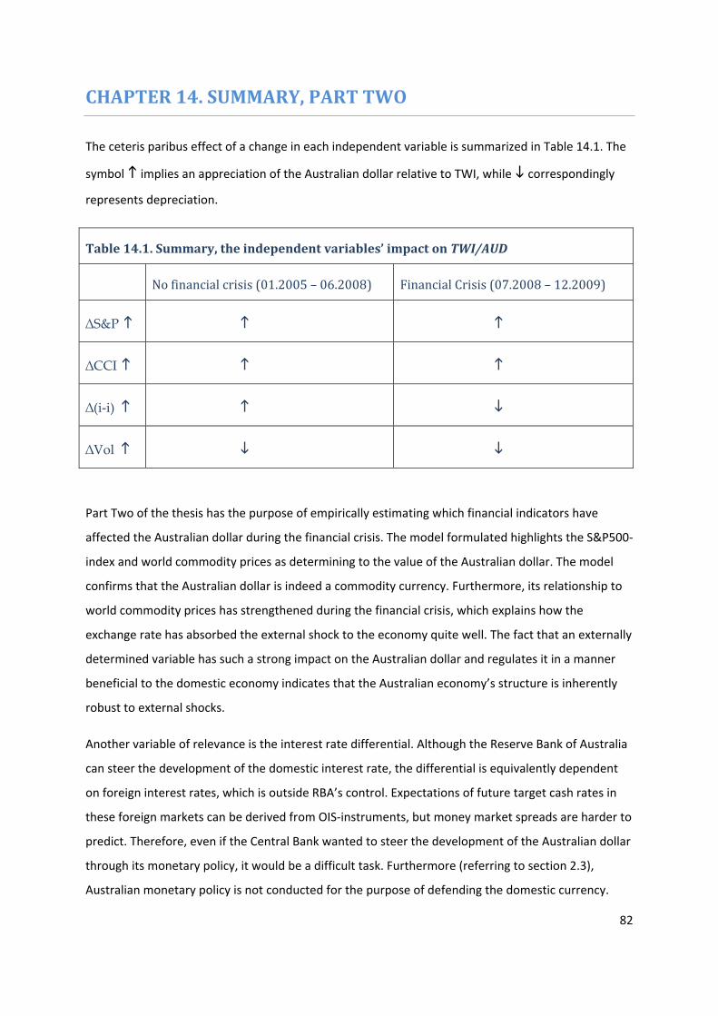
82
CHAPTER 14. SUMMARY, PART TWO
The ceteris paribus effect of a change in each independent variable is summarized in Table 14.1. The
symbol implies an appreciation of the Australian dollar relative to TWI, while correspondingly
represents depreciation.
Table 14.1. Summary, the independent variables’ impact on TWI/AUD
No financial crisis (01.2005 – 06.2008) Financial Crisis (07.2008 – 12.2009)
∆S&P
∆CCI
∆(i‐i)
∆Vol
Part Two of the thesis has the purpose of empirically estimating which financial indicators have
affected the Australian dollar during the financial crisis. The model formulated highlights the S&P500‐
index and world commodity prices as determining to the value of the Australian dollar. The model
confirms that the Australian dollar is indeed a commodity currency. Furthermore, its relationship to
world commodity prices has strengthened during the financial crisis, which explains how the
exchange rate has absorbed the external shock to the economy quite well. The fact that an externally
determined variable has such a strong impact on the Australian dollar and regulates it in a manner
beneficial to the domestic economy indicates that the Australian economy’s structure is inherently
robust to external shocks.
Another variable of relevance is the interest rate differential. Although the Reserve Bank of Australia
can steer the development of the domestic interest rate, the differential is equivalently dependent
on foreign interest rates, which is outside RBA’s control. Expectations of future target cash rates in
these foreign markets can be derived from OIS‐instruments, but money market spreads are harder to
predict. Therefore, even if the Central Bank wanted to steer the development of the Australian dollar
through its monetary policy, it would be a difficult task. Furthermore (referring to section 2.3),
Australian monetary policy is not conducted for the purpose of defending the domestic currency.
83
Conclusively, the interest rate differential is outside the nation’s control. However, its impact on the
Australian dollar has changed during the financial crisis, and it is therefore not structurally robust in
the same sense as the with the S&P 500‐index and world commodity prices.
The final variable affecting the exchange rate is the implied (expected) volatility in the Australian
dollar. The effect of this variable has increased during the financial crisis. The volatility measure is not
a fundamental factor with respect to the development of the Australian dollar, and the relationship is
therefore not beneficial to the domestic real economy. The other three independent variables have
displayed large fluctuations during the financial crisis, and this has caused the Australian dollar
volatility to increase. Combined with the larger impact of volatility during the crisis, this has created a
negative spiral for the value of the Australian dollar. This justifies the sterilized intervention the
Reserve Bank of Australia conducted towards the end of 2008. It also implies that the Australian
dollar, left to its own devices, might not completely absorb shocks to the economy. One situation
where this is the case is when a global economic recession is accompanied by high volatility in
financial markets.
84
CHAPTER 15. CONCLUSION
This thesis was written with the objective of revealing why Australia has handled the most recent
financial crisis so much better than most other developed nations. The two parts constituting the
thesis have differed in approach, but share this objective. Before the final conclusion is reached, a
repetition of the problem formulation is appropriate:
Why did the Australian economy cope so well with the 2007/2008 global financial crisis?
First and foremost, the Australian financial system has not experienced any severe dislocation, unlike
many other nations. This is both due to the Australian business model of conservative balance sheet
management, as well as the effective monetary policy conducted by the Reserve Bank of Australia.
In the context of the real domestic economy, flexibility is the word best explaining the favourable
outcome. Without this trait, the adjustments made necessary by the financial crisis would not have
been viable. The Australian Government has supported the domestic economy through fiscal policy
measures, and although it is disputable how effective these measures have been, it has certainly
helped ease stress in the economy caused by the uncertain economic outlook.
In addition to an inherently flexible and resilient domestic economy, Australia’s composition and role
in international trade has been an important factor explaining the fortunate outcome. The role as a
small, commodity‐exporting country and the strong trade relations to Asia has underpinned the
economic survival of Australia throughout the crisis.
Even with all the above traits present, the situation would have been much more severe if the
exchange rate had not absorbed part of the external shock. In Part Two, a strong relationship
between the Australian dollar and world commodity prices was confirmed empirically. This
relationship further helps stabilize domestic economic activity.
The favourable outcome can not be entirely ascribed to the domestic policy response, nor was it
caused by sheer luck. A combination of the characteristics mentioned above has been the ultimate
reason why Australia survived the financial crisis without any major problems.
85
REFERENCES
Books, articles and webpages
Australian Financial Markets Association. Media Release. Published 15.01.2010.
http://www.afma.com.au/ (12.05.2010)
Australian Government Centrelink (2009): Household Stimulus Package.
http://www.centrelink.gov.au/internet/internet.nsf/individuals/bonus_payments_feb2009.htm
(28.04.2010)
Australian Government Department of Foreign Affairs and Trade (2009): Composition of Trade
Australia 2008‐09. Commonwealth of Australia Publications.
Australian Office of Financial Management. Role and Function.
http://www.aofm.gov.au/content/role.asp (12.05.2010)
Ball, Laurence (1991): The Genesis of Inflation and the Costs of Disinflation. NBER Working Paper. No.
3621.
Bank of International Settlements (2007): Triennial Central Bank Survey of Foreign Exchange and
Derivatives Market Activity in April 2007 – Preliminary Global Results – Turnover. Published
25.09.2007.
http://www.bis.org/press/p070925.htm (15.04.2010)
BBC News (2009): Timeline: Credit Crunch to Downturn. Last updated 07.08.2009.
http://news.bbc.co.uk/2/hi/7521250.stm (28.04.2010)
Blinder, Alan S. (1988): The Fall and Rise of Keynesian Economics. Economic Record. December 1988.
Vol 64, pp. 278‐294.
Business Monitor International (2010): Australia Business Forecast Report. Q2 2010. Don’t Count on
The Recovery. Business Monitor International Ltd, UK.
86
Chen, Yu‐chin and Kenneth Rogoff (2003): Commodity Currencies. Journal of International Economics.
May 2003. Vol. 60, pp. 133‐160.
Dungey, Mardi (2001): International Shocks and the Role of Domestic Policy in Australia. Centre for
Economic Reseach Discussion Paper. No. 443.
Engel, Charles (2000): Long‐Run PPP May Not Hold After All. Journal of International Economics. August 2000. Vol. 51, pp. 243‐273.
Engle, Robert F. and Clive W.J. Granger (1987): Co‐integration and Error Correction: Representation,
Estimation and Testing. Econometrica. March 1987. Vol. 55, pp. 251‐276.
Ergas, Henry (2009): Five reasons why a Rudd fiscal stimulus may not work. Published by The
Australian 09.02.2009.
http://www.theaustralian.com.au/news/stimulus‐may‐not‐work/story‐e6frg7b6‐1111118793315
(08.06.2010)
Frenkel, Jacob A. (1976): A Monetary Approach to the Exchange Rate: Doctrinal Aspects and Empirical
Evidence. Scandinavian Journal of Economics. Vol. 78 pp. 200‐224.
Frenkel, Jacob A. (1981): Flexible Exchange Rates, Prices, and the Role of ‘News’. Lessons from the
1970s. Journal of Political Economy. August 1981. Vol. 89, pp. 665‐705.
Gärtner, Manfred (2006): Macroeconomics. 2nd Ed. Prentice Hall, USA.
Granger, Clive W.J. and Paul Newbold (1974). Spurious Regressions in Econometrics. Journal of
Econometrics. July 1974. Vol. 2, pp. 111‐120.
Gruen, David W.R. and Jenny Wilkinson (1994): Australia’s Real Exchange Rate: Is It Explained by the
Terms of Trade or by Real Interest Rate Differentials? The Economic Record. June 1994. Vol. 70, pp.
204‐219.
Hatzinikolaou, Dimitris and Metodey Ploasek (2005): The Commodity Currency View of the Australian
Dollar: A Multivariate Cointegration Approach. Journal of Applied Economics. May 2005. Vol. 8, pp.
81‐99.
87
Hodrick, Robert J. (1987): The Empirical Evidence on the Efficiency of Forward and Futures Foreign
Exchange Markets. Harwood Academic Publishers, Switzerland.
International Monetary Fund (2009): Balance of Payments and International Investment Position
Manual. 6th ed. IMF Publication Services, USA.
Isard, Peter (1995): Exchange Rate Economics. Cambridge University Press, UK.
Ito, Takatoshi (1990): Foreign Exchange Rate Expectations: Micro Survey Data. American Economic
Review. June 1990. Vol. 80, pp. 434‐449.
Karfakis, Costas and Anthony Phipps (1999): Modeling the Australian Dollar – US Dollar Exchange
Rate Using Cointegration Techniques. Review of International Economics. May 1999. Vol. 7, pp. 265‐
279.
King, Alan (1998): Uncovered Interest Parity: New Zealand’s Post‐Deregulation Experience. Applied
Financial Economics. October 1998. Vol. 8, pp. 495‐503.
King, Mervyn (2002): No Money, No Inflation – The Role of Money in the Economy. Bank of England
Quarterly Bulletin. Summer 2002. pp. 162‐177.
Kremers, Jeroen J.M, Neil R. Ericsson and Juan J. Dolado (1992): The Power of Cointegration Tests.
Board of Governors of the Federal Reserve System. International Finance Discussion Papers. June
1992. No. 431.
Leigh, Andrew K. (2009): How Much Did the 2009 Fiscal Stimulus Boost Spending? Evidence From a
Household Survey. Published by Australian National University, CAMA Working Papers. No. 2009‐22.
MacDonald, Ronald and Mark P. Taylor (1991): The Monetary Approach to the Exchange Rate: Long‐
Run Relationships and Coefficient Restrictions. Economics Letters. October 1991. Vol. 37, pp. 179‐
185.
Meese, Richard A. (1986): Empirical Assessment of Foreign Currency Risk Premiums. Published by the
Federal Reserve Bank of St.Louis, Proceedings. pp. 157‐180.
88
Meese, Richard A. and Kevin Rogoff (1983): Empirical Exchange Rate Models of the Seventies: Do
They Fit Out of Sample? Journal of International Economics. February 1983. Vol. 14, pp. 3‐24.
Mendenhall, William and Terry Sincich (2003): A Second Course in Statistics. Regression Analysis. 6th
ed. Prentice Hall, USA.
Moosa, Imad and Razzaque H. Bhatti (1997): International Parity Conditions: Theory, Econometric
Testing and Empirical Evidence. Palgrave Macmillan, UK.
Moosa, Imad (2006): International Finance. An Analytical Approach. 2nd ed. McGraw Hill, Australia.
Mussa, Michael (1979): Empirical Regularities in the Behaviour of Exchange Rates and Theories of the
Foreign Exchange Market. Carnegie‐Rochester Conference Series on Public Policy. January 1979. Vol.
11, pp. 9‐57.
OECD Factbook (2009): Population and Migration.
http://puck.sourceoecd.org/pdf/factbook2009/302009011e‐01‐01‐01.pdf (17.03.2010)
The Reserve Bank of Australia. Financial Stability.
http://www.rba.gov.au/fin‐stability/index.html
The Reserve Bank of Australia.Market Operations.
http://www.rba.gov.au/mkt‐operations/index.html
The Reserve Bank of Australia. Monetary Policy.
http://www.rba.gov.au/monetary‐policy/index.html
The Reserve Bank of Australia Publications:
Financial Stability Review. September 2008.
Financial Stability Review. September 2009.
Financial Stability Review. March 2010.
Statement on Monetary Policy. 11 February 2008.
Statement on Monetary Policy. 10 November 2008.
Statement on Monetary Policy. 6 November 2009.
89
Statement on Monetary Policy. February 2010.
http://www.rba.gov.au/publications/
Roberts, Russel (2008): Economist: Don’t Jump the Gun on Stimulus Plan. Published by NPR
16.01.2008
http://www.npr.org/templates/story/story.php?storyId=18159629 (22.04.2010)
Sarno, Lucio and Mark P. Taylor (2006): The economics of exchange rates. Cambridge University
Press, UK.
Savin, N.Eugene and Kenneth J. White (1977): The Durbin‐Watson Test for Serial Correlation with
Extreme Sample Sizes or Many Regressors. Econometrica. November 1977. Vol. 45, pp. 1989‐1996.
Standard & Poors. Indices – S&P500.
http://www.standardandpoors.com/indices/sp‐500/en/us/?indexId=spusa‐500‐usduf‐‐p‐us‐l‐‐
(03.05.2010)
Takàts, Elöd and Patrizia Tumbarello (2009): Australian Bank and Corporate Sector Vulnerabilities –
An International Perspective. IMF Working Paper. No. 09/223.
Thomson Reuters. Equal Weight Continuous Commodity Index (CCI) Factsheet. February 2010.
http://thomsonreuters.com/content/financial/pdf/i_and_a/indices/cci_factsheet.pdf (25.03.2010)
Tumbarello, Patrizia (2010): Australian, New Zealand Banks Remain Sound During Global Crisis.
Published by IMF Survey Magazine 22.02.2010.
http://www.imf.org/external/pubs/ft/survey/so/2010/car012210a.htm (17.04.2010)
Twome, Brian (2009): Why China’s Currency Tangos With The USD. Published by Investopedia
http://www.investopedia.com/articles/forex/09/chinas‐peg‐to‐the‐dollar.asp (12.05.2010)
Wooldridge, Jeffrey (2006): Introductory Econometrics. A modern Approach. 3rd ed. Thomson South‐
Western, USA.
World Trade Organization (2009): International Trade Statistics 2009.
WTO Publications, Geneva.
90
Data
Australian Bureau of Statistics. Composition of Australian exports.
www.abs.gov.au. Catalogue number 5368.0
Australian Bureau of Statistics. Retail trade, Australia.
www.abs.gov.au Catalogue number 8501.0
Reserve Bank of Australia. Daily and monthly exchange rates.
http://www.rba.gov.au/statistics/tables/index.html#exchange_rates (10.02.2010)
Reserve Bank of Australia.
Consumer Price Index.
RBA Index of Commodity Prices.
http://www.rba.gov.au/statistics/tables/index.html#prices_inflation (10.02.2010)
Reserve Bank of Australia. Interest rates.
http://www.rba.gov.au/statistics/tables/index.html#interest_rates (10.02.2010)
Reserve Bank of Australia. Equity prices.
http://www.rba.gov.au/statistics/tables/index.html#share_mkts (10.02.2010)
Reserve Bank of Australia. Australian Government budget.
http://www.rba.gov.au/statistics/tables/index.html#govt_finance (10.02.2010)
Reserve Bank of Australia.
Indicators of spending and confidence.
Gross Domestic Product.
http://www.rba.gov.au/statistics/tables/index.html#output_labour (10.02.2010)
Reserve Bank of Australia. International real GDP.
http://www.rba.gov.au/statistics/tables/index.html#overseas (10.02.2010)
Reserve Bank of Australia. Monthly exports and imports.
http://www.rba.gov.au/statistics/tables/index.html#balance_payments (10.02.2010)
91
Standard & Poor’s. ASX200 daily index values.
http://www.standardandpoors.com/indices/sp‐asx‐200/en/us/?indexId=spausta200audff‐‐p‐au‐‐‐‐
(10.02.2010)
Standard & Poor’s. S&P500 daily index values.
http://www.standardandpoors.com/indices/sp‐500/en/us/?indexId=spusa‐500‐usduf‐‐p‐us‐l‐‐
(10.02.2010)
Thomson Reuters Datastream (accessed from the NHH Library).
Daily CCI‐index values.
3 month implied volatility, Australian dollar.
Consumer Price Indices; Japan, UK, USA and Germany.
Interest rates; Australia, Japan, UK, USA and Germany.
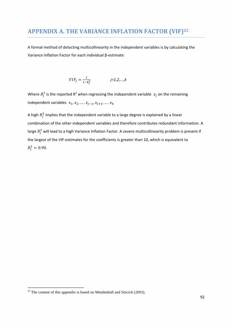
92
APPENDIX A. THE VARIANCE INFLATION FACTOR (VIF)22
A formal method of detecting multicollinearity in the independent variables is by calculating the
Variance Inflation Factor for each individual β‐estimate:
j=1,2,...,k
Where is the reported R2 when regressing the independent variable on the remaining
independent variables , , … . , , … .
A high implies that the independent variable to a large degree is explained by a linear
combination of the other independent variables and therefore contributes redundant information. A
large will lead to a high Variance Inflation Factor. A severe multicollinearity problem is present if
the largest of the VIF‐estimates for the coefficients is greater than 10, which is equivalent to
0.90.
22 The content of this appendix is based on Mendenhall and Sincich (2003).
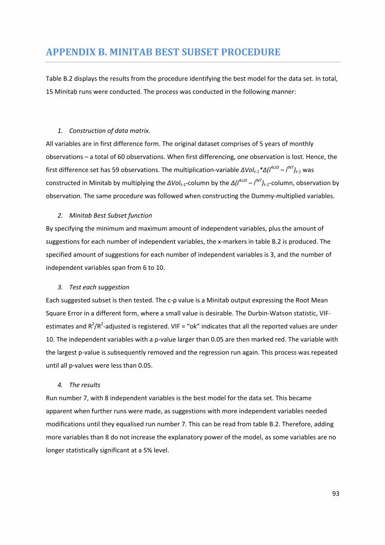
93
APPENDIX B. MINITAB BEST SUBSET PROCEDURE
Table B.2 displays the results from the procedure identifying the best model for the data set. In total,
15 Minitab runs were conducted. The process was conducted in the following manner:
1. Construction of data matrix.
All variables are in first difference form. The original dataset comprises of 5 years of monthly
observations – a total of 60 observations. When first differencing, one observation is lost. Hence, the
first difference set has 59 observations. The multiplication‐variable ∆Volt‐1*∆(iAUD – iINT)t‐1 was
constructed in Minitab by multiplying the ∆Volt‐1‐column by the ∆(iAUD – iINT)t‐1‐column, observation by
observation. The same procedure was followed when constructing the Dummy‐multiplied variables.
2. Minitab Best Subset function
By specifying the minimum and maximum amount of independent variables, plus the amount of
suggestions for each number of independent variables, the x‐markers in table B.2 is produced. The
specified amount of suggestions for each number of independent variables is 3, and the number of
independent variables span from 6 to 10.
3. Test each suggestion
Each suggested subset is then tested. The c‐p value is a Minitab output expressing the Root Mean
Square Error in a different form, where a small value is desirable. The Durbin‐Watson statistic, VIF‐
estimates and R2/R2‐adjusted is registered. VIF = “ok” indicates that all the reported values are under
10. The independent variables with a p‐value larger than 0.05 are then marked red. The variable with
the largest p‐value is subsequently removed and the regression run again. This process was repeated
until all p‐values were less than 0.05.
4. The results
Run number 7, with 8 independent variables is the best model for the data set. This became
apparent when further runs were made, as suggestions with more independent variables needed
modifications until they equalised run number 7. This can be read from table B.2. Therefore, adding
more variables than 8 do not increase the explanatory power of the model, as some variables are no
longer statistically significant at a 5% level.
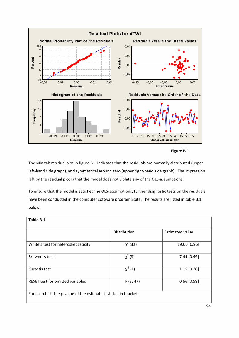
94
Residual
Per
cent
0,040,020,00-0,02-0,04
99,9
99
90
50
10
1
0,1
Fitted Value
Res
idua
l
0,050,00-0,05-0,10-0,15
0,04
0,02
0,00
-0,02
Residual
Freq
uenc
y
0,0240,0120,000-0,012-0,024
16
12
8
4
0
Observation Order
Res
idua
l
5550454035302520151051
0,04
0,02
0,00
-0,02
Normal Probability Plot of the Residuals Residuals Versus the Fitted Values
Histogram of the Residuals Residuals Versus the Order of the Data
Residual Plots for dTWI
Figure B.1
The Minitab residual plot in figure B.1 indicates that the residuals are normally distributed (upper
left‐hand side graph), and symmetrical around zero (upper right‐hand side graph). The impression
left by the residual plot is that the model does not violate any of the OLS‐assumptions.
To ensure that the model is satisfies the OLS‐assumptions, further diagnostic tests on the residuals
have been conducted in the computer software program Stata. The results are listed in table B.1
below.
Table B.1
Distribution Estimated value
White’s test for heteroskedasticity χ2 (32) 19.60 [0.96]
Skewness test χ2 (8) 7.44 [0.49]
Kurtosis test χ 2 (1) 1.15 [0.28]
RESET test for omitted variables F (3, 47) 0.66 [0.58]
For each test, the p‐value of the estimate is stated in brackets.

95
For each test, the null hypothesis is that there is no presence of the OLS‐violation it tests for, and the
estimated p‐values indicate that the null hypothesis cannot be rejected at a 5% significance level for
any of the tests. Therefore, it is presumed that the model is well‐specified and the estimated
coefficients unbiased.
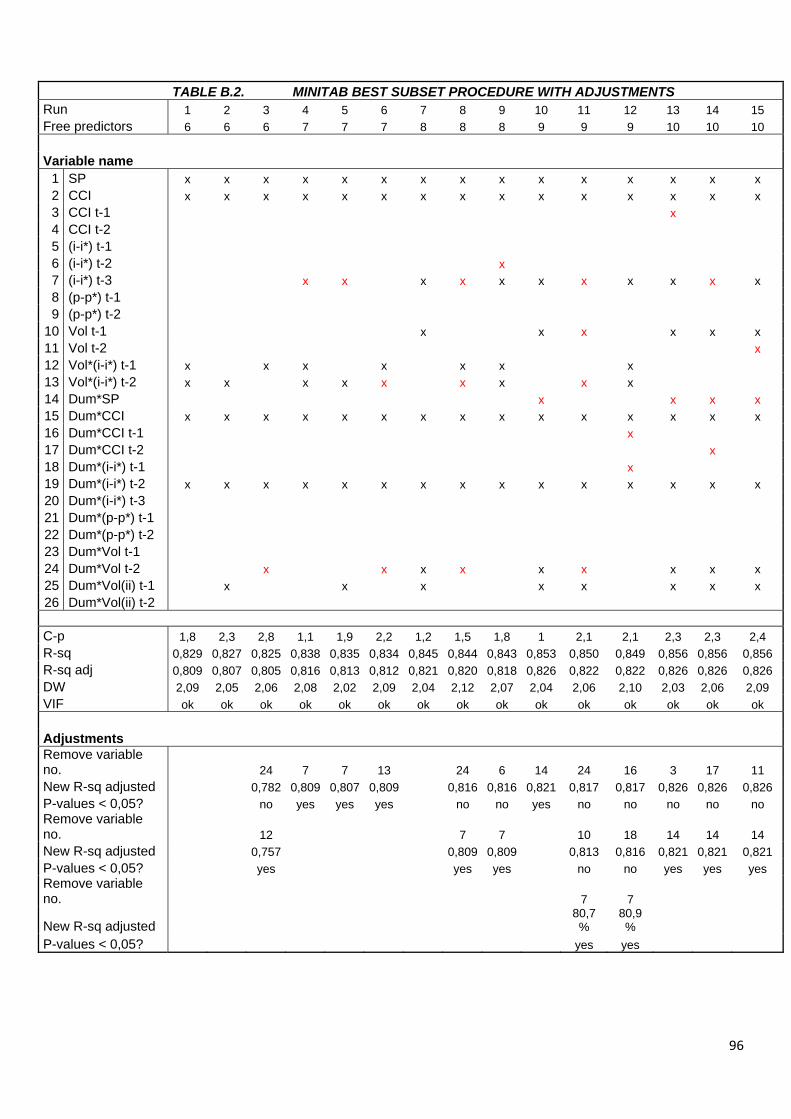
96
TABLE B.2. MINITAB BEST SUBSET PROCEDURE WITH ADJUSTMENTS Run 1 2 3 4 5 6 7 8 9 10 11 12 13 14 15 Free predictors 6 6 6 7 7 7 8 8 8 9 9 9 10 10 10 Variable name
1 SP x x x x x x x x x x x x x x x 2 CCI x x x x x x x x x x x x x x x 3 CCI t-1 x 4 CCI t-2 5 (i-i*) t-1 6 (i-i*) t-2 x 7 (i-i*) t-3 x x x x x x x x x x x 8 (p-p*) t-1 9 (p-p*) t-2
10 Vol t-1 x x x x x x 11 Vol t-2 x 12 Vol*(i-i*) t-1 x x x x x x x 13 Vol*(i-i*) t-2 x x x x x x x x x 14 Dum*SP x x x x 15 Dum*CCI x x x x x x x x x x x x x x x 16 Dum*CCI t-1 x 17 Dum*CCI t-2 x 18 Dum*(i-i*) t-1 x 19 Dum*(i-i*) t-2 x x x x x x x x x x x x x x x 20 Dum*(i-i*) t-3 21 Dum*(p-p*) t-1 22 Dum*(p-p*) t-2 23 Dum*Vol t-1 24 Dum*Vol t-2 x x x x x x x x x 25 Dum*Vol(ii) t-1 x x x x x x x x 26 Dum*Vol(ii) t-2 C-p 1,8 2,3 2,8 1,1 1,9 2,2 1,2 1,5 1,8 1 2,1 2,1 2,3 2,3 2,4 R-sq 0,829 0,827 0,825 0,838 0,835 0,834 0,845 0,844 0,843 0,853 0,850 0,849 0,856 0,856 0,856 R-sq adj 0,809 0,807 0,805 0,816 0,813 0,812 0,821 0,820 0,818 0,826 0,822 0,822 0,826 0,826 0,826 DW 2,09 2,05 2,06 2,08 2,02 2,09 2,04 2,12 2,07 2,04 2,06 2,10 2,03 2,06 2,09 VIF ok ok ok ok ok ok ok ok ok ok ok ok ok ok ok Adjustments Remove variable no. 24 7 7 13 24 6 14 24 16 3 17 11 New R-sq adjusted 0,782 0,809 0,807 0,809 0,816 0,816 0,821 0,817 0,817 0,826 0,826 0,826 P-values < 0,05? no yes yes yes no no yes no no no no no Remove variable no. 12 7 7 10 18 14 14 14 New R-sq adjusted 0,757 0,809 0,809 0,813 0,816 0,821 0,821 0,821 P-values < 0,05? yes yes yes no no yes yes yes Remove variable no. 7 7
New R-sq adjusted 80,7 %
80,9 %
P-values < 0,05? yes yes