Ausplots Training - Session 3
69
-
Upload
bensparrowau -
Category
Environment
-
view
63 -
download
6
Transcript of Ausplots Training - Session 3


The “After Lunch” Session 3
( we’ll be watching for anyone nodding off!)
Topics to cover:
Locating the plot/ plot layout/PositioningPoint InterceptBasal wedgeVegetation Structural SummaryGeneral Site info

MethodLocating the PlotPlot LayoutPositioning

Locating the Site
12
3
4 & 56
7

Locating the Site – Community 1
12
3
4 & 56
7

Heterogeneous
Not Community 1Heterogeneous
Locating Plots – Community 1

Locating the Site – Community 2
12
3
4 & 56
7

Locating Plots – Community 2
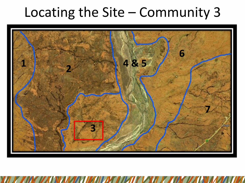
Locating the Site – Community 3
12
3
4 & 56
7

Locating Plots - Community 3
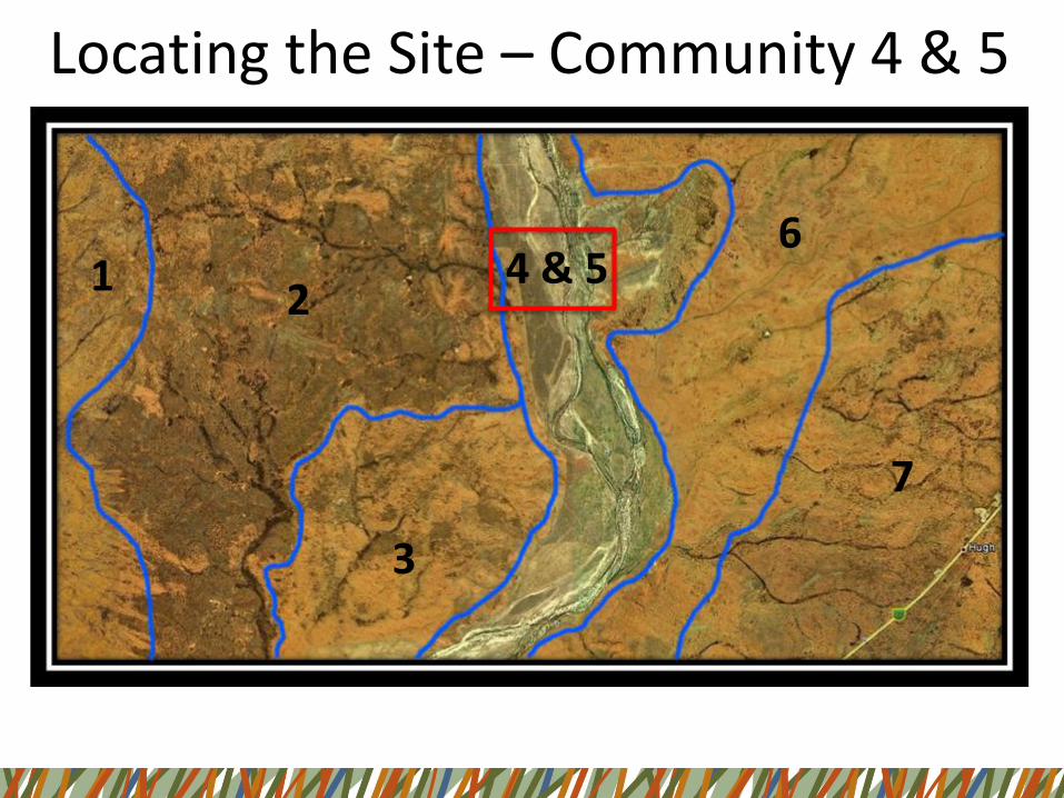
Locating the Site – Community 4 & 5
12
3
4 & 56
7

Locating Plots - Community 4 & 5

Locating the Site – Community 6
12
3
4 & 56
7

Locating Plots – Community 6

Locating the Site – Community 7
12
3
4 & 56
7

Locating Plots – Community 7

Exceptions

Where to put sites
• Homogeneous or constantly mixed (Veg, Slope, relief, soil)
• Aligned to grid
• 100x100 (1ha)
• Avoid roads, cattleyards, fences, bores etc.
• Consider access nowand in the future

Plot Layout

Naming Conventions
A AusPlots T Transects L LTERN
S Supersites G General use TRA Training
Australian Capital Territory CT New South Wales NS
Northern Territory NT Queensland QD
South Australia SA Tasmania TC
Victoria VC Western Australia WA
Arnhem Coast ARC Arnhem Plateau ARP Broken Hill Complex BHC
Burt Plain BRT Cape York Peninsula CYP Carnarvon CAR
Central Arnhem CA Central Kimberley CK Central Ranges CR
Two Letters for State, One letter for Type – Three letters for Bioregion – Four numbers to identify the plot number.
Here would be:
SAS-MDD-0001 (South Australia Supersites – Murray Darling Depression – plot #1)
State Code:
Plot Type:
Bioregion code:

Using the DGPS: an Overview
• Turn on and connect both units
• Well before you intend to use
•Remember to charge batteries

Actual process will be run through in the field.
Process involves
– Ensuring set up is correct
– Taking a reference point
– Placing a pre-determined grid over the reference point
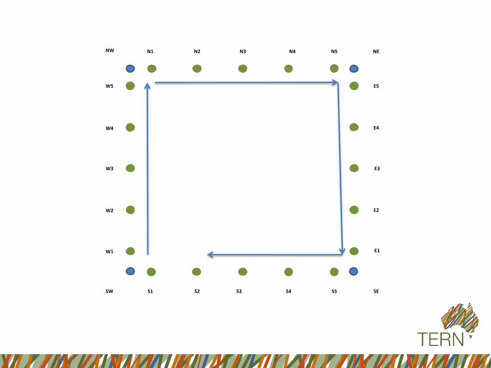
– Using the grid to peg out the plot corners, transect ends and the centre point.
– Recording all of these points
– Downloading them in the office
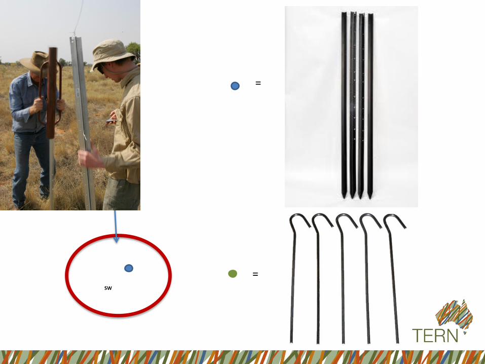
SW
=
=
Start

W3
W2
W1
SW
S1
NEN5N4N3N2N1NW
W5
W4
W3
W2
W1
SW S2 S3 S4 S5 SE
E1
E2
E3
E4
E5

S1
NEN5N4N3N2N1NW
W5
W4
W3
W2
W1
SW S2 S3 S4 S5 SE
E1
E2
E3
E4
E5
C

S1
NEN5N4N3N2N1NW
W5
W4
W3
W2
W1
SW S2 S3 S4 S5 SE
E1
E2
E3
E4
E5

MethodPoint Intercept

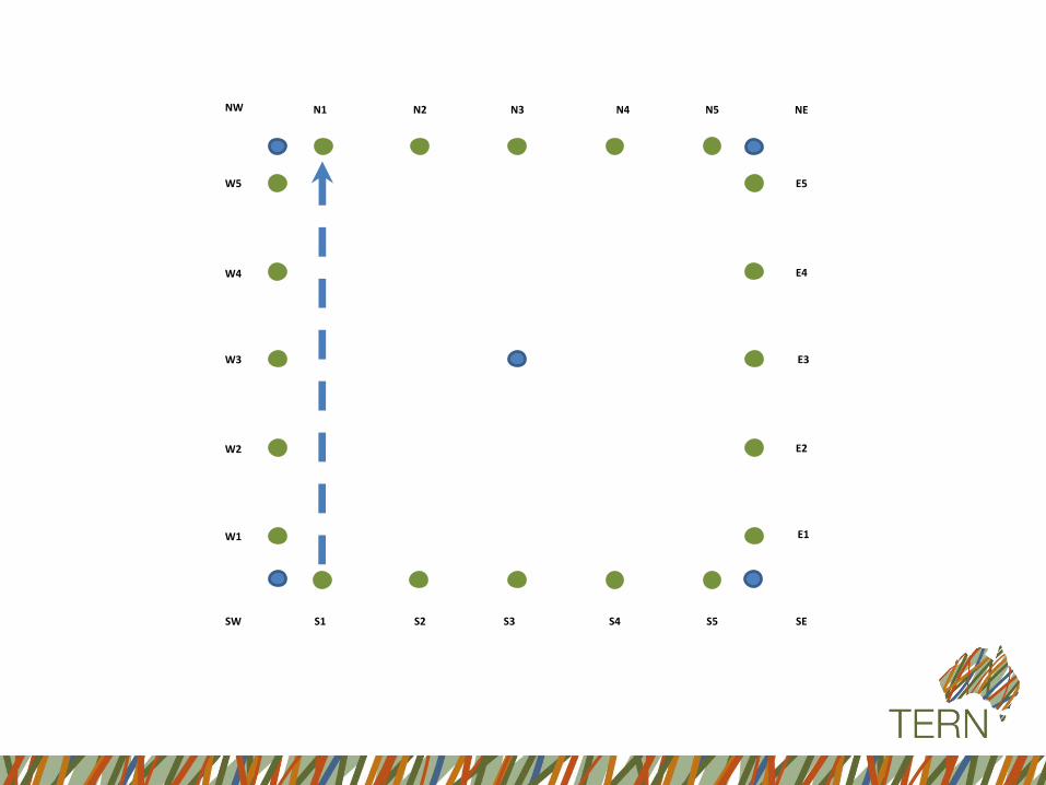
Point intercept
• An repeatable objective quantitative measure of both vegetation presence, and percentage cover within the quadrat
• Essential to determine change
• Based on a huge number of references
– All agree 1000pts minimum
• 10 x 100m transects with a sample every 1 m
– 5 transects N-S, 5 transects E-W
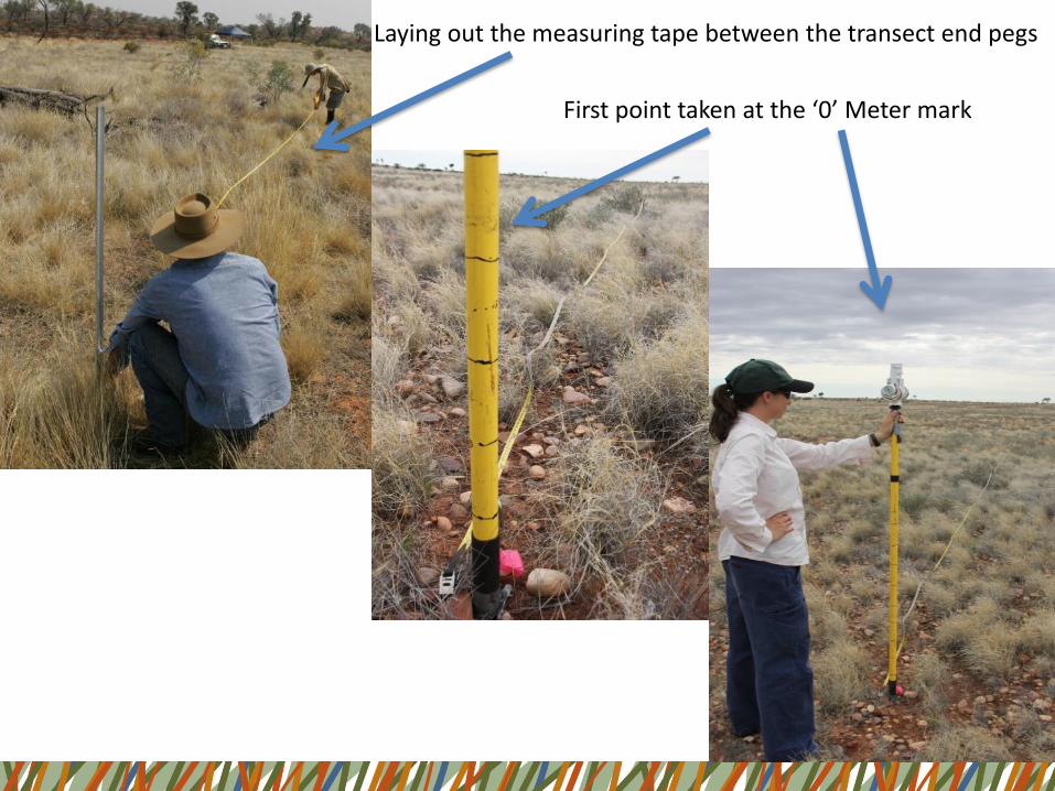
Laying out the measuring tape between the transect end pegs
First point taken at the ‘0’ Meter mark

Densiometer
Graduated Staff
Laser Pointer
Field Cover Assessment Device (Gandalf’s Staff)
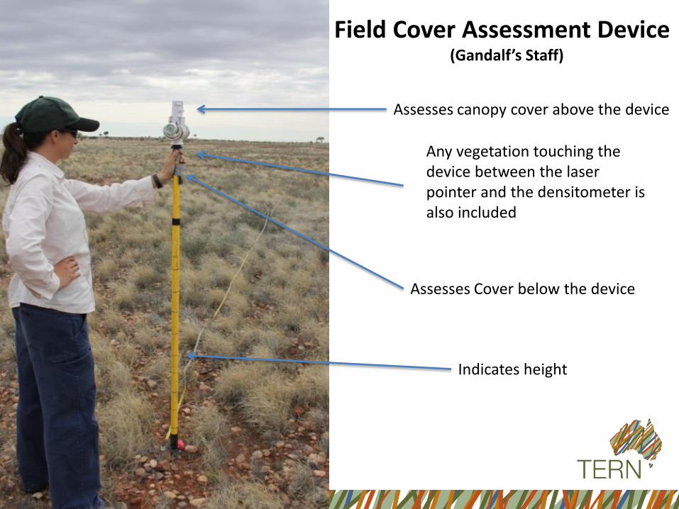
Assesses canopy cover above the device
Indicates height
Assesses Cover below the device
Field Cover Assessment Device (Gandalf’s Staff)
Any vegetation touching the device between the laser pointer and the densitometer is also included

In this example the substrate is litter as that is what the laser is intersecting
Height is read from the staff

Assessing Cover above the device
• Uses a densitometer
• Ensure the device is level using the bubble level
• Use the cross hairs and small circle to identify what is
intersected.

The Concept of “In Canopy – Sky”
• Needed so that the data is readily convertible between ‘Opaque Canopy Cover’ And ‘Foliage Projective Cover’(FPC)
• Makes the same data useful for more applications
• Opaque canopy cover assumes that the canopy is solid
• FPC only counts cover where the vertical projection of foliage obscures the ground.
• Uses the densitometer

In Canopy Sky
A Vegetation Intersectfor Eucalyptus Sp.
“In Canopy- Sky” for Eucalyptus Sp.

No Intersect
In Canopy - Sky
Eucalyptus sp.

No Intersects in this area

The “Laser”

A Laser Intersect with Substrate - Litter

A Laser intersect with Bare Ground

S1
NEN5N4N3N2N1NW
W5
W4
W3
W2
W1
SW S2 S3 S4 S5 SE
E1
E2
E3
E4
E5

S1
NEN5N4N3N2N1NW
W5
W4
W3
W2
W1
SW S2 S3 S4 S5 SE
E1
E2
E3
E4
E5

S1
NEN5N4N3N2N1NW
W5
W4
W3
W2
W1
SW S2 S3 S4 S5 SE
E1
E2
E3
E4
E5

S1
NEN5N4N3N2N1NW
W5
W4
W3
W2
W1
SW S2 S3 S4 S5 SE
E1
E2
E3
E4
E5

S1
NEN5N4N3N2N1NW
W5
W4
W3
W2
W1
SW S2 S3 S4 S5 SE
E1
E2
E3
E4
E5


MethodUsing the Basal Wedge

Basal area
• A plotless measure
• Works on a Circular Plot assessing circular trunks
• Works plotlessly because the area of the plot varies at the same RATE as the increase in basal area needed to get a hit with increasing distance. (Area of plot V’s area of Basal area)
• Calculations a little complex
• Well accepted and rapid method.

• For a given basal area factor.
• Take the number of “hits”
• Multiply by the basal area factor
• Answer in M2/ha
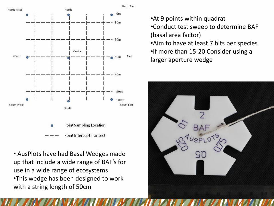
•At 9 points within quadrat•Conduct test sweep to determine BAF (basal area factor)•Aim to have at least 7 hits per species•If more than 15-20 Consider using a larger aperture wedge
• AusPlots have had Basal Wedges made up that include a wide range of BAF’s for use in a wide range of ecosystems•This wedge has been designed to work with a string length of 50cm

•Place the String Knot (indicates 50cm) directly underneath you preferred eye.•Sight through a wedge gap •Spin on the spot through 360 degrees ensuring you are aware of your start point.•Possible (but unlikely) to have different BAF for different species at the one sweep point.•Rotate the wedge to determine the appropriate BAF for your environment.
Squinting definitely helps you to look this silly!

The tree is clearly wider than the wedge aperture – This is counted as a hit of 1
The tree is exactly the same width as the wedge aperture – This is counted as a hit of 0.5
The tree here is clearly narrower than the wedge aperture – this is not counted as a hit at all.


MethodStructural Summary
• Aim to be able to create level 5 NVIS –Association Level
– Requires Dominant Growth Form, height, Cover and species (3) for the three traditional strata (Upper, Mid and Ground)
– Much of this information is already collected within the method/on the app
– Only need to collect the interpretive information that not collected elsewhere.

• Collect – Dominant 3 species in each strata in the app in decreasing order of cover.
• This info then used to query other components of the data
– Calculate Cover for each of the species
– Calculate average height for that species in the strata.
– Determine dominant growth form for that species at that site.
– Use height profiles to confirm strata.


Ground Layer
Cenchrus cilliaris - 1

Mid Layer
Senna artemisioides ssp. Filifolia - 1

Upper LayerAcacia aneura – 1Acacia estrophiolata – 2Hakea divaricata - 3

Emergent Layer
Acacia estrophiolata - 1

Three most dominant species nominated in each
strata, in decreasing order of cover

MethodGeneral Site Info

The bare basics!
• To provide data context
• Observers
• Plot ID e.g. SAA-STP-00001
• IBRA Bioregion
• Date
• MGA & datum
• Grid layout/alignment
• Mud map

The bare basics!
• Landform pattern
• Landform element
• Site slope (degrees from horizontal)
• Site Aspect (degrees from north)
• Outcrop lithology e.g. Quartzite
• Surface strew size
• Location comments and general comments .e.g. recent rain