Audio Engineering Society Convention Paper - XLR Techs (2005-10 AES... · Audio Engineering Society...
47
Audio Engineering Society Convention Paper Presented at the 119th Convention 2005 October 7–10 New York, New York USA This convention paper has been reproduced from the author's advance manuscript, without editing, corrections, or consideration by the Review Board. The AES takes no responsibility for the contents. Additional papers may be obtained by sending request and remittance to Audio Engineering Society, 60 East 42P nd P Street, New York, New York 10165-2520, USA; also see www.aes.org. All rights reserved. Reproduction of this paper, or any portion thereof, is not permitted without direct permission from the Journal of the Audio Engineering Society. Ground-Plane Constant Beamwidth Transducer (CBT) Loudspeaker Circular-Arc Line Arrays D. B. (Don) Keele, Jr.P 1 P, Douglas J. Button P 2 P P 1 P Harman International Industries, Northridge, California, 91329, USA [email protected] P 2 PJBL Professional, Northridge, California, 91329, USA [email protected] ABSTRACT This paper describes a design variation of the CBT loudspeaker line array that is intended to operate very close to a planar reflecting surface. The original free-standing CBT array is halved lengthwise and then positioned close to a flat surface so that acoustic reflections essentially recreate the missing half of the array. This halved array can then be doubled in size which forms an array which is double the height of the original array. When compared to the original free-standing array, the ground-plane CBT array provides several advantages including: 1. elimination of detrimental floor reflections, 2. doubles array height, 3. doubles array sensitivity, 4. doubles array maximum SPL capability, 5. extends vertical beamwidth control down an octave, and 6. minimizes near-far variation of SPL. This paper explores these characteristics through sound-field simulations and over-the-ground-plane measurements of three systems: 1. a conventional two-way compact monitor, 2. an experimental un-shaded straight-line array, and 3. an experimental CBT Legendre-shaded circular-arc curved-line array. 1. INTRODUCTION Ground-plane radio-frequency antennas have been around for many decades. The common whip antenna is nothing more than one half of a dipole mounted against a flat electro-magnetic reflecting surface. This “ground- plane” provides a reflective image that effectively creates the missing half of the dipole. For antennas, a ground plane may consist of a natural (e.g., Earth or sea) surface, an artificial surface such as the roof of a motor vehicle, or a specially designed artificial surface. Loudspeakers are commonly designed to operate best in free-space without the aid of reflective surfaces but are often located near large planar surfaces. These surfaces generate reflections that can detrimentally modify the speaker’s frequency response and radiation pattern. With few exceptions, most speakers are not designed to operate next to a ground plane.
Transcript of Audio Engineering Society Convention Paper - XLR Techs (2005-10 AES... · Audio Engineering Society...
Audio Engineering Society
Convention Paper Presented at the 119th Convention
2005 October 7–10 New York, New York USA
This convention paper has been reproduced from the author's advance manuscript, without editing, corrections, or consideration by the Review Board. The AES takes no responsibility for the contents. Additional papers may be obtained by sending request and remittance to Audio Engineering Society, 60 East 42P
ndP Street, New York, New York 10165-2520, USA; also see www.aes.org.
All rights reserved. Reproduction of this paper, or any portion thereof, is not permitted without direct permission from the Journal of the Audio Engineering Society.
Ground-Plane Constant Beamwidth Transducer (CBT) Loudspeaker Circular-Arc Line Arrays
D. B. (Don) Keele, Jr.P
1P, Douglas J. Button P
2P
P
1P Harman International Industries, Northridge, California, 91329, USA
P
2 PJBL Professional, Northridge, California, 91329, USA
ABSTRACT
This paper describes a design variation of the CBT loudspeaker line array that is intended to operate very close to a planar reflecting surface. The original free-standing CBT array is halved lengthwise and then positioned close to a flat surface so that acoustic reflections essentially recreate the missing half of the array. This halved array can then be doubled in size which forms an array which is double the height of the original array. When compared to the original free-standing array, the ground-plane CBT array provides several advantages including: 1. elimination of detrimental floor reflections, 2. doubles array height, 3. doubles array sensitivity, 4. doubles array maximum SPL capability, 5. extends vertical beamwidth control down an octave, and 6. minimizes near-far variation of SPL. This paper explores these characteristics through sound-field simulations and over-the-ground-plane measurements of three systems: 1. a conventional two-way compact monitor, 2. an experimental un-shaded straight-line array, and 3. an experimental CBT Legendre-shaded circular-arc curved-line array.
1. INTRODUCTION Ground-plane radio-frequency antennas have been around for many decades. The common whip antenna is nothing more than one half of a dipole mounted against a flat electro-magnetic reflecting surface. This “ground-plane” provides a reflective image that effectively creates the missing half of the dipole. For antennas, a ground plane may consist of a natural (e.g., Earth or sea) surface, an artificial surface such as the roof of a motor vehicle, or a specially designed artificial surface.
Loudspeakers are commonly designed to operate best in free-space without the aid of reflective surfaces but are often located near large planar surfaces. These surfaces generate reflections that can detrimentally modify the speaker’s frequency response and radiation pattern. With few exceptions, most speakers are not designed to operate next to a ground plane.
Keele and Button Ground-Plane CBT Loudspeaker Line Arrays
AES 119th Convention, New York, New York, 2005 October 7–10 Page 2 of 47
Conventional CBT circular-arc line arrays are designed to be used free standing and operate best when not near any large reflecting surfaces. This paper describes a design variation of the CBT loudspeaker line array called a ground-plane CBT array that is specifically designed to operate when placed against a planar reflective boundary. The variation consists of a modified array that is intended to operate near or very close to a single acoustic reflecting surface, such as a floor, wall, or ceiling.
The modification consists of splitting the original free-standing CBT array in half lengthwise, and then positioning the “halved” array close to the reflecting surface so that the acoustic reflections essentially recreate the missing half of the array. The “halved” array can then be doubled in size making its height equal to the original free-standing array. This double-size half array and its acoustic reflection in the ground plane effectively forms an array double the height of the original free-standing array.
This effective doubling of size positively impacts several performance characteristics of the ground-plane CBT array which are outlined in the following list and described in more detail in a later section (Sec. 5).
1. Eliminates detrimental floor reflections. 2. Doubles array height. 3. Doubles array sensitivity (+6 dB). 4. Doubles array maximum sound pressure level
(SPL) capability (+6 dB). 5. Extends operating bandwidth down by an
octave (or two depending on how the beamwidth is defined).
6. Minimizes near-far variation of SPL.
Of course, these performance advantages can be applied to create a ground-plane array that is one-half the size of a free-standing array that provides the same performance as the full-size free-standing array when a ground plane is available.
1.1. A Brief CBT History CBT or constant beamwidth transducer theory is based on un-classified military under-water transducer research done in the late 1970s and early 80s [1 - 3]. This research describes a curved-surface transducer in the form of a spherical cap with frequency-independent Legendre shading that provides wide-band extremely-constant beamwidth and directivity behavior with virtually no side lobes.
The theory was applied to loudspeaker arrays by Keele in 2000 [4] where he extended the concept to arrays based on circular-arc line arrays and toroidal-shaped curved surface arrays. Keele also extended the concept to straight-line and flat-panel CBT arrays with the use of signal delays [5]. The 3D sound-field of CBT circular-arc line arrays was analyzed by Keele in 2003 [6]. In 2003 Keele also described the practical implementation of CBT circular-arc line arrays [7].
1.2. Paper Organization
This paper is organized as follows: Section 1 (this one) briefly reviews CBT arrays and introduces the concept of the ground-plane array and describes a number of its advantages. Section 2 outlines the steps to create a ground-plane array from a free-standing array. Section 3 describes simulations of a number of different types of arrays primarily through the display of vertical-plane sound-fields.
Measurements are described in section 4 by showing the results of a series of ground-plane frequency responses taken as a function of height, distance, and angle. These measurements were done on a conventional two-way compact-monitor system, and on two experimental arrays: an un-shaded straight-line array and a CBT Legendre-shaded circular-arc curved-line array. Section 5 goes into more detail about the advantages of the ground-plane CBT array and section 6 concludes.
2. STEPS TO CREATE A GROUND-PLANE ARRAY FROM A FREE-STANDING ARRAY
This section outlines the steps to create a ground-plane array from a free-standing array.
A free-standing vertically-oriented CBT line-array is shown in Fig. 1.

Keele and Button Ground-Plane CBT Loudspeaker Line Arrays
AES 119th Convention, New York, New York, 2005 October 7–10 Page 3 of 47
Fig. 1. Free-standing circular-arc CBT line-array design. The example array is drawn assuming a 90º arc with 40 loudspeakers.
Figure 2 shows the array of Fig. 1 located with its bottom against a planar sound-reflecting ground-plane surface.
Fig. 2. Free-standing CBT array located over ground plane.
Figure 3 shows the same array along with its acoustic reflection image in the ground plane. Effectively, a vertical stack of two arrays has been created. The acoustic output of the two arrays will interfere with each other and significantly change the vertical radiation pattern of the original free-standing array.
Fig. 3. Free-standing CBT array located over ground plane with acoustic reflection.
Figure 4 shows the array of Fig. 2 with its bottom half removed.
Fig. 4. Free-standing CBT array with bottom half of array removed.
Keele and Button Ground-Plane CBT Loudspeaker Line Arrays
AES 119th Convention, New York, New York, 2005 October 7–10 Page 4 of 47
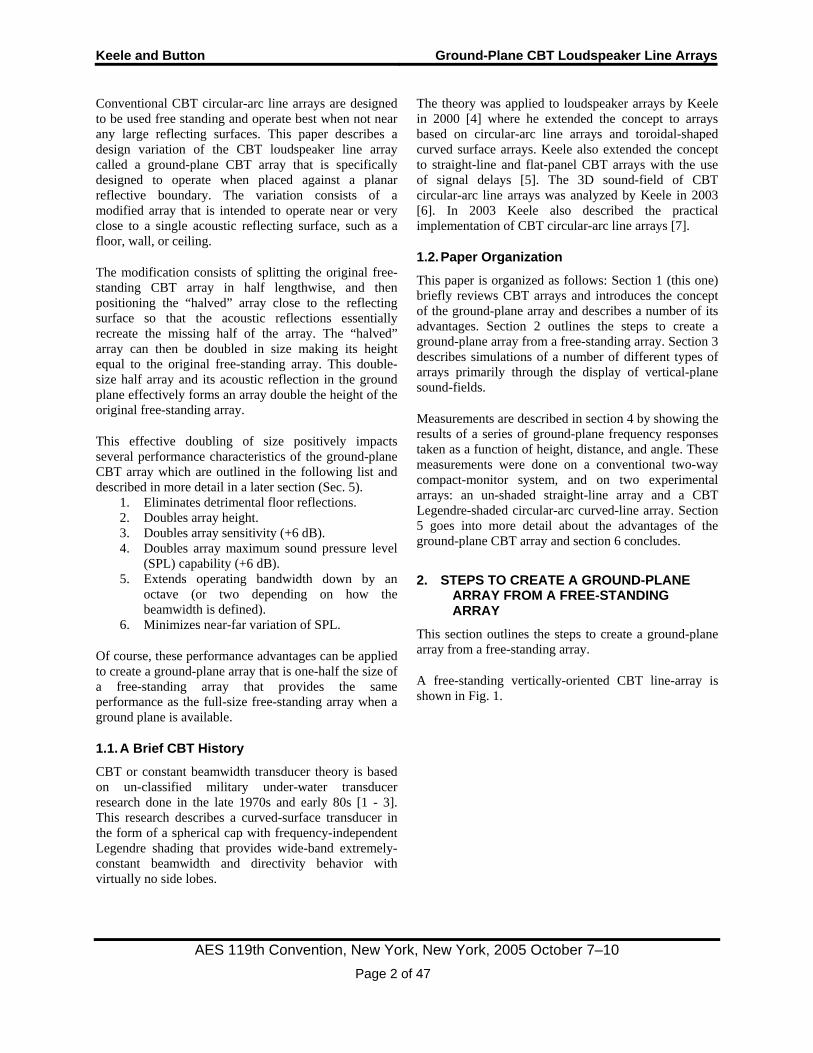
Figure 5 shows the upper half of the array lowered so that its bottom lies on the ground plane.
Fig. 5. The CBT array of Fig. 4 lowered so that bottom surface is resting on the ground plane. The example array is now a 45º arc and contains 20 drivers.
This half-size array can then be doubled in height to equal the size of the original free-standing array and is shown in Fig. 6.
Fig. 6. The CBT array of Fig. 5 doubled in height with the same number of drivers but half the angle as the free-standing array of Fig. 1. The array now is 45º and has 40 drivers.
The example array now is a 45º arc and contains 40 drivers. When this array’s acoustic reflection in the ground-plane is considered (Fig. 7), a double-height array is formed as compared to the original free-standing array of Fig. 1. This double-size array effectively controls vertical coverage down an octave lower than the original array and also effectively eliminates detrimental reflections from the ground plane.
Side note: if the angular coverage of the array is defined as its coverage angle above the ground plane only, the operating frequency of the ground-plane CBT array effectively drops by two octaves rather than one, as compared to the free-standing array. This is because the ground-plane CBT array height has doubled and its coverage angle has halved (by definition), as compared to the free-standing array.
Fig. 7. The CBT array of Fig, 6 with ground-plane reflection. Note that the array with its reflection now effectively forms a single array that is double the height of the free-standing array of Fig. 1 and contains double the number of drivers (80 each). This array with ground-plane reflection now operates an octave lower than the free-standing CBT array of Fig. 1 (or two octaves depending on how beamwidth is defined).
Keele and Button Ground-Plane CBT Loudspeaker Line Arrays
AES 119th Convention, New York, New York, 2005 October 7–10 Page 5 of 47
3. SOUND-FIELD SIMULATIONS
3.1. Description Contrary to the three previous CBT papers [4 – 6] which primarily calculated and displayed far-field parameters such as beamwidth, directivity, polar response, and polar balloons; this paper instead investigates the near-field pressure distribution of the arrays via simulated vertical-plane sound fields..
The point-source array simulator program used in [4 - 6] was used to predict the 2D vertical sound-field pressure magnitude distribution of the various arrays described in this paper. This program calculates the complex pressure at a particular distance and location for a 3-D array of point sources of arbitrary magnitude and phase.
The pressure distribution was calculated in the plane of the array in a 3 m (height) by 4 m (length) region with the source located in the lower left corner of the region. The perfectly-reflective ground plane extends horizontally across the bottom of the region at zero height. Pressure magnitudes were calculated at octave intervals from 32 Hz (or 125 Hz) to 16 kHz over a region of 161 points horizontal and 121 points vertical, making a total of 19,481 points. The points were evenly-spaced at about 25 mm (1”).
The above-ground-plane pressure distribution was calculated by using the image source method [8] assuming only a single perfectly-reflective rigid planar surface. Effectively this creates a single composite array composed of both the above-ground actual array and the below-ground mirror image of the array.
3.1.1. Color Coding of dB Pressure Level
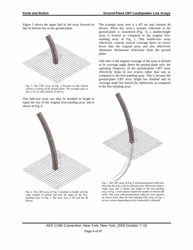
All the 2D simulated sound-fields in this paper are color coded in a yellow-hot scheme in dB sound pressure level according to the scale shown in Fig.8. Levels are normalized to the sound pressure that the array generates at one meter on axis if all the sources are on and in phase (0 dB). Levels higher than +10 dB are coded in full yellow while levels less than -40 dB are full black.
Fig. 8. Color scale used for the simulated sound-field plots. The scale covers a 50 dB range. The scale varies smoothly from high-level yellow at +10 dB (right), through mid-level red at –15 dB (middle), to low-level black at -40 dB (left).
3.1.2. Isobar Contour Lines
Constant-pressure 3dB-increment contour lines were added to all the sound-field plots. The first contour starts at +9 dB and the last contour stops at -39 dB.
3.2. Arrays Simulated The vertical sound fields of the following point-source configurations were simulated:
1. A single point source located above a non-reflective ground plane (free space).
2. A single point source located above a perfectly-reflective ground plane.
3. A vertically-oriented straight-line source with and without Hann shading located resting on a perfectly-reflective ground plane.
4. A circular-arc curved-line source with and without Legendre shading located with its bottom resting on a perfectly-reflective ground plane. The former is a physically-curved CBT array [4].
5. A delay-curved straight-line source with and without Legendre shading located resting on perfectly-reflective ground plane. The former is a delay-curved CBT array [5].
The straight- and curved-line sources were 1.25 m (50 inches) high and contained 50 point sources spaced about 25.4 mm (1”) apart.. The curved arrays were either physically- or delay-curved to form an arc of 45º.
3.3. Shading Shading refers to frequency-independent magnitude-only changes in level (attenuation) that are applied to each of the drivers of the array. Shading dramatically reduces the array’s side lobes and improves off-axis frequency responses. Typically, the center sources of an array are driven at full level and then each source’s level is smoothly reduced the farther it is from the center of the array. The sources at the ends of the array have highest attenuation.
Keele and Button Ground-Plane CBT Loudspeaker Line Arrays
AES 119th Convention, New York, New York, 2005 October 7–10 Page 6 of 47
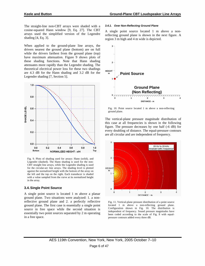
The straight-line non-CBT arrays were shaded with a cosine-squared Hann window [9, Eq. 27]. The CBT arrays used the simplified version of the Legendre shading [4, Eq. 3].
When applied to the ground-plane line arrays, the drivers nearest the ground plane (bottom) are on full while the drivers farthest from the ground plane (top) have maximum attenuation. Figure 9 shows plots of these shading functions. Note that Hann shading attenuates more rapidly than the Legendre shading. The theoretical electrical power loss for these two shadings are 4.3 dB for the Hann shading and 3.2 dB for the Legendre shading [7, Section 5].
Fig. 9. Plots of shading used for arrays: Hann (solid), and Legendre (dashed). The Hann shading is used for the non-CBT straight line arrays, while the Legendre shading is used for the circular-arc line arrays. The shading level is plotted against the normalized height with the bottom of the array on the left and the top on the right. Each transducer is shaded with a value sampled from the curve at its normalized height in the array.
3.4. Single Point Source
A single point source is located 1 m above a planar ground plane. Two situations were analyzed: 1. a non-reflective ground plane and 2. a perfectly reflective ground plane. The first case is essentially a single point source in free space while the second situation is essentially two point sources separated by 2 m operating in a free space.
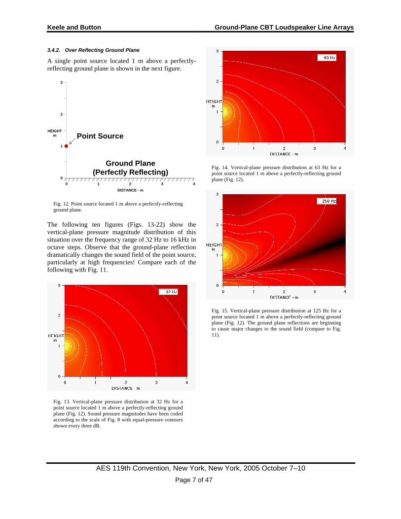
3.4.1. Over Non-Reflecting Ground Plane
A single point source located 1 m above a non-reflecting ground plane is shown in the next figure. A region 3 m high and 4 m wide is depicted.
0 1 2 3 4DISTANCE - m
HEIGHTm
0
1
2
3
Ground Plane(Non Reflecting)
Point Source
Fig. 10. Point source located 1 m above a non-reflecting ground plane.
The vertical-plane pressure magnitude distribution of this case at all frequencies is shown in the following figure. The pressure decreases by one half (-6 dB) for every doubling of distance. The equal-pressure contours are all circular and are independent of frequency.
Fig. 11. Vertical-plane pressure distribution of a point source located 1 m above a non-reflecting ground plane. Configuration shown in Fig. 10. The distribution is independent of frequency. Sound pressure magnitudes have been coded according to the scale of Fig. 8 with equal-pressure contours added every three dB.
Keele and Button Ground-Plane CBT Loudspeaker Line Arrays
AES 119th Convention, New York, New York, 2005 October 7–10 Page 7 of 47
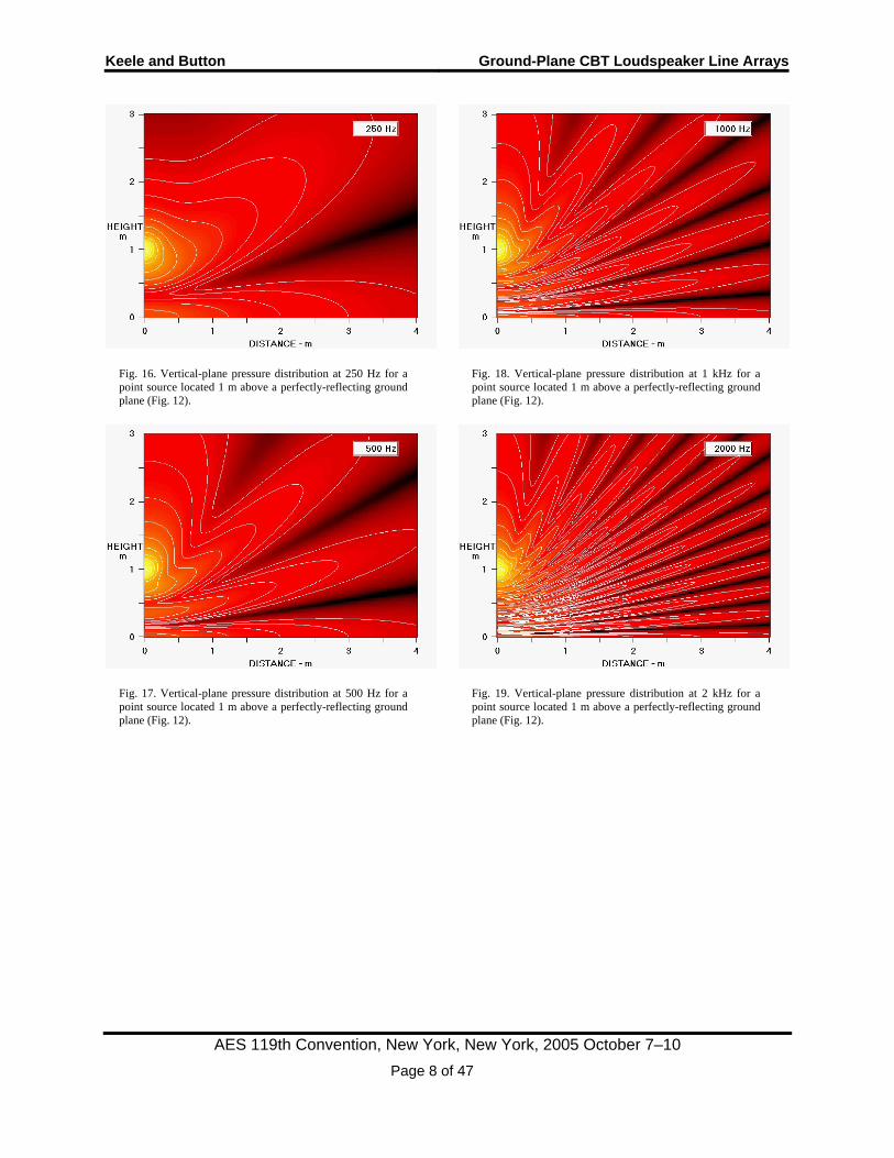
3.4.2. Over Reflecting Ground Plane
A single point source located 1 m above a perfectly-reflecting ground plane is shown in the next figure.
0 1 2 3 4DISTANCE - m
HEIGHTm
0
1
2
3
Ground Plane(Perfectly Reflecting)
Point Source
Fig. 12. Point source located 1 m above a perfectly-reflecting ground plane.
The following ten figures (Figs. 13-22) show the vertical-plane pressure magnitude distribution of this situation over the frequency range of 32 Hz to 16 kHz in octave steps. Observe that the ground-plane reflection dramatically changes the sound field of the point source, particularly at high frequencies! Compare each of the following with Fig. 11.
Fig. 13. Vertical-plane pressure distribution at 32 Hz for a point source located 1 m above a perfectly-reflecting ground plane (Fig. 12). Sound pressure magnitudes have been coded according to the scale of Fig. 8 with equal-pressure contours shown every three dB.
Fig. 14. Vertical-plane pressure distribution at 63 Hz for a point source located 1 m above a perfectly-reflecting ground plane (Fig. 12).
Fig. 15. Vertical-plane pressure distribution at 125 Hz for a point source located 1 m above a perfectly-reflecting ground plane (Fig. 12). The ground plane reflections are beginning to cause major changes to the sound field (compare to Fig. 11).
Keele and Button Ground-Plane CBT Loudspeaker Line Arrays
AES 119th Convention, New York, New York, 2005 October 7–10 Page 8 of 47
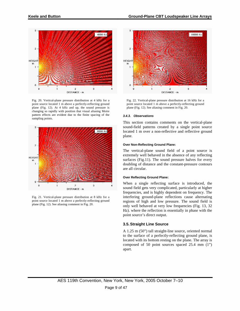
Fig. 16. Vertical-plane pressure distribution at 250 Hz for a point source located 1 m above a perfectly-reflecting ground plane (Fig. 12).
Fig. 17. Vertical-plane pressure distribution at 500 Hz for a point source located 1 m above a perfectly-reflecting ground plane (Fig. 12).
Fig. 18. Vertical-plane pressure distribution at 1 kHz for a point source located 1 m above a perfectly-reflecting ground plane (Fig. 12).
Fig. 19. Vertical-plane pressure distribution at 2 kHz for a point source located 1 m above a perfectly-reflecting ground plane (Fig. 12).
Keele and Button Ground-Plane CBT Loudspeaker Line Arrays
AES 119th Convention, New York, New York, 2005 October 7–10 Page 9 of 47
Fig. 20. Vertical-plane pressure distribution at 4 kHz for a point source located 1 m above a perfectly-reflecting ground plane (Fig. 12). At 4 kHz and up, the sound pressure is changing so rapidly with position that visual aliasing Moire pattern effects are evident due to the finite spacing of the sampling points.
Fig. 21. Vertical-plane pressure distribution at 8 kHz for a point source located 1 m above a perfectly-reflecting ground plane (Fig. 12). See aliasing comment in Fig. 20.
Fig. 22. Vertical-plane pressure distribution at 16 kHz for a point source located 1 m above a perfectly-reflecting ground plane (Fig. 12). See aliasing comment in Fig. 20.
3.4.3. Observations
This section contains comments on the vertical-plane sound-field patterns created by a single point source located 1 m over a non-reflective and reflective ground plane.
Over Non-Reflecting Ground Plane:
The vertical-plane sound field of a point source is extremely well behaved in the absence of any reflecting surfaces (Fig.11). The sound pressure halves for every doubling of distance and the constant-pressure contours are all circular.
Over Reflecting Ground Plane:
When a single reflecting surface is introduced, the sound field gets very complicated, particularly at higher frequencies, and is highly dependent on frequency. The interfering ground-plane reflections cause alternating regions of high and low pressure. The sound field is only well behaved at very low frequencies (Fig. 13, 32 Hz). where the reflection is essentially in phase with the point source’s direct output.
3.5. Straight Line Source
A 1.25 m (50”) tall straight-line source, oriented normal to the surface of a perfectly-reflecting ground plane, is located with its bottom resting on the plane. The array is composed of 50 point sources spaced 25.4 mm (1”) apart.
Keele and Button Ground-Plane CBT Loudspeaker Line Arrays
AES 119th Convention, New York, New York, 2005 October 7–10 Page 10 of 47
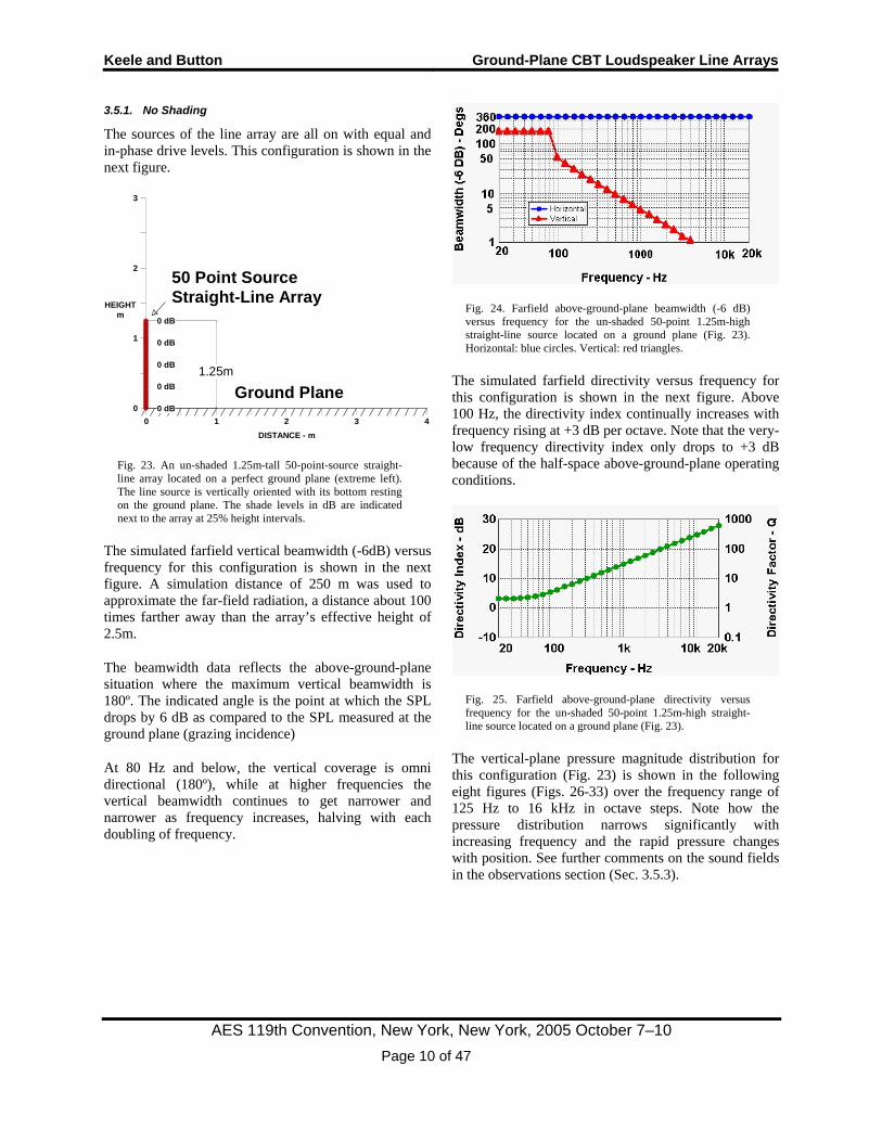
3.5.1. No Shading
The sources of the line array are all on with equal and in-phase drive levels. This configuration is shown in the next figure.
0 1 2 3 4DISTANCE - m
HEIGHTm
0
1
2
3
Ground Plane
50 Point SourceStraight-Line Array
1.25m
0 dB
0 dB
0 dB
0 dB
0 dB
Fig. 23. An un-shaded 1.25m-tall 50-point-source straight-line array located on a perfect ground plane (extreme left). The line source is vertically oriented with its bottom resting on the ground plane. The shade levels in dB are indicated next to the array at 25% height intervals.
The simulated farfield vertical beamwidth (-6dB) versus frequency for this configuration is shown in the next figure. A simulation distance of 250 m was used to approximate the far-field radiation, a distance about 100 times farther away than the array’s effective height of 2.5m.
The beamwidth data reflects the above-ground-plane situation where the maximum vertical beamwidth is 180º. The indicated angle is the point at which the SPL drops by 6 dB as compared to the SPL measured at the ground plane (grazing incidence)
At 80 Hz and below, the vertical coverage is omni directional (180º), while at higher frequencies the vertical beamwidth continues to get narrower and narrower as frequency increases, halving with each doubling of frequency.
Fig. 24. Farfield above-ground-plane beamwidth (-6 dB) versus frequency for the un-shaded 50-point 1.25m-high straight-line source located on a ground plane (Fig. 23). Horizontal: blue circles. Vertical: red triangles.
The simulated farfield directivity versus frequency for this configuration is shown in the next figure. Above 100 Hz, the directivity index continually increases with frequency rising at +3 dB per octave. Note that the very-low frequency directivity index only drops to +3 dB because of the half-space above-ground-plane operating conditions.
Fig. 25. Farfield above-ground-plane directivity versus frequency for the un-shaded 50-point 1.25m-high straight-line source located on a ground plane (Fig. 23).
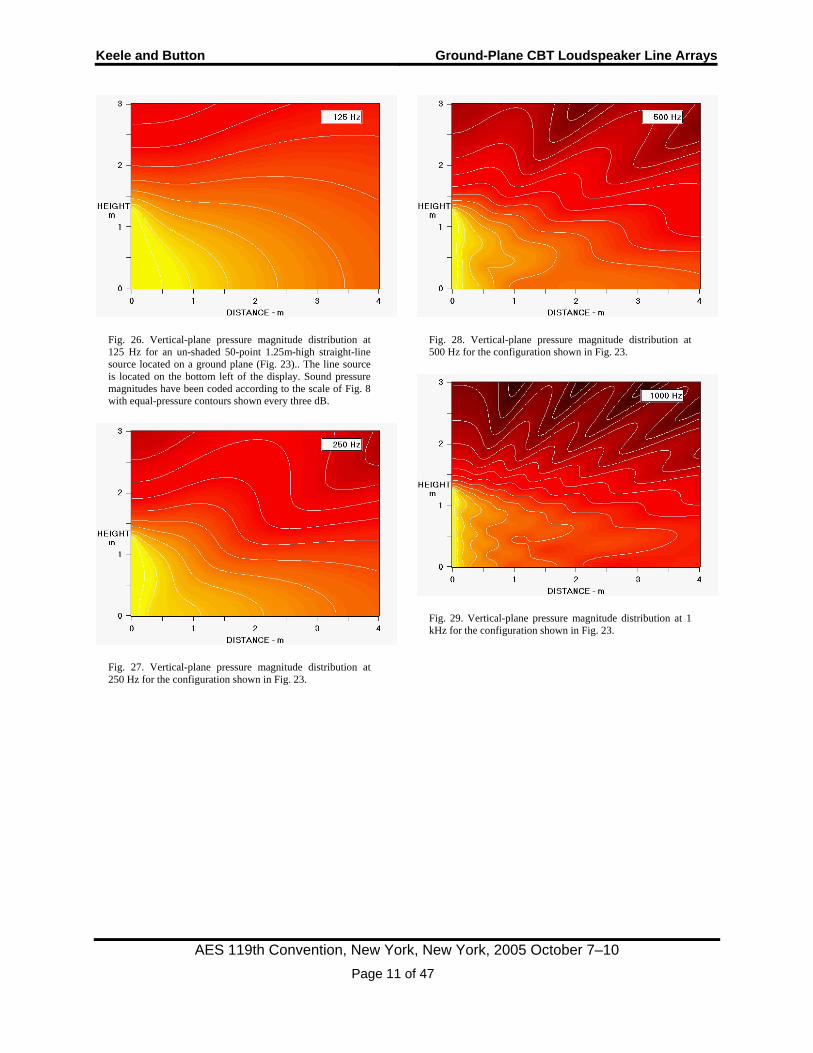
The vertical-plane pressure magnitude distribution for this configuration (Fig. 23) is shown in the following eight figures (Figs. 26-33) over the frequency range of 125 Hz to 16 kHz in octave steps. Note how the pressure distribution narrows significantly with increasing frequency and the rapid pressure changes with position. See further comments on the sound fields in the observations section (Sec. 3.5.3).
Keele and Button Ground-Plane CBT Loudspeaker Line Arrays
AES 119th Convention, New York, New York, 2005 October 7–10 Page 11 of 47
Fig. 26. Vertical-plane pressure magnitude distribution at 125 Hz for an un-shaded 50-point 1.25m-high straight-line source located on a ground plane (Fig. 23).. The line source is located on the bottom left of the display. Sound pressure magnitudes have been coded according to the scale of Fig. 8 with equal-pressure contours shown every three dB.
Fig. 27. Vertical-plane pressure magnitude distribution at 250 Hz for the configuration shown in Fig. 23.
Fig. 28. Vertical-plane pressure magnitude distribution at 500 Hz for the configuration shown in Fig. 23.
Fig. 29. Vertical-plane pressure magnitude distribution at 1 kHz for the configuration shown in Fig. 23.
Keele and Button Ground-Plane CBT Loudspeaker Line Arrays
AES 119th Convention, New York, New York, 2005 October 7–10 Page 12 of 47
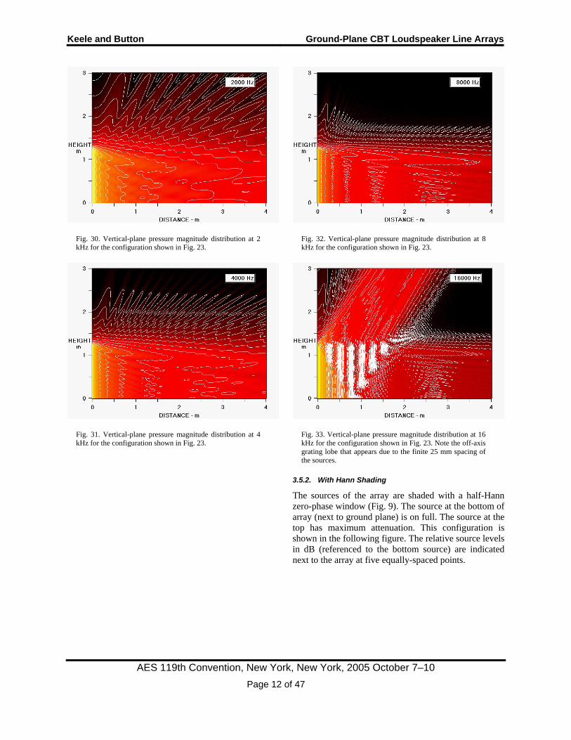
Fig. 30. Vertical-plane pressure magnitude distribution at 2 kHz for the configuration shown in Fig. 23.
Fig. 31. Vertical-plane pressure magnitude distribution at 4 kHz for the configuration shown in Fig. 23.
Fig. 32. Vertical-plane pressure magnitude distribution at 8 kHz for the configuration shown in Fig. 23.
Fig. 33. Vertical-plane pressure magnitude distribution at 16 kHz for the configuration shown in Fig. 23. Note the off-axis grating lobe that appears due to the finite 25 mm spacing of the sources.
3.5.2. With Hann Shading
The sources of the array are shaded with a half-Hann zero-phase window (Fig. 9). The source at the bottom of array (next to ground plane) is on full. The source at the top has maximum attenuation. This configuration is shown in the following figure. The relative source levels in dB (referenced to the bottom source) are indicated next to the array at five equally-spaced points.
Keele and Button Ground-Plane CBT Loudspeaker Line Arrays
AES 119th Convention, New York, New York, 2005 October 7–10 Page 13 of 47
0 1 2 3 4DISTANCE - m
HEIGHTm
0
1
2
3
Ground Plane
50 Point SourceStraight-Line Array
1.25m
0 dB
-6.0 dB
-1.4 dB
-16.8 dB
-INF dB
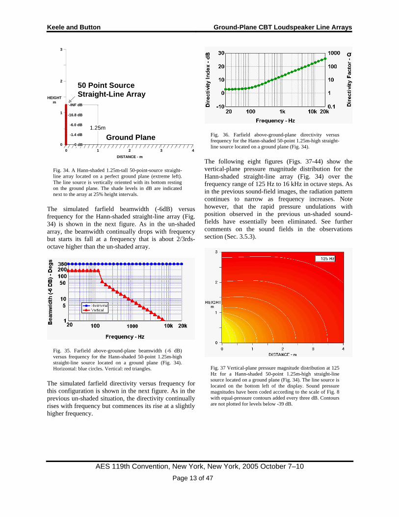
Fig. 34. A Hann-shaded 1.25m-tall 50-point-source straight-line array located on a perfect ground plane (extreme left). The line source is vertically oriented with its bottom resting on the ground plane. The shade levels in dB are indicated next to the array at 25% height intervals.
The simulated farfield beamwidth (-6dB) versus frequency for the Hann-shaded straight-line array (Fig. 34) is shown in the next figure. As in the un-shaded array, the beamwidth continually drops with frequency but starts its fall at a frequency that is about 2/3rds-octave higher than the un-shaded array.
Fig. 35. Farfield above-ground-plane beamwidth (-6 dB) versus frequency for the Hann-shaded 50-point 1.25m-high straight-line source located on a ground plane (Fig. 34). Horizontal: blue circles. Vertical: red triangles.
The simulated farfield directivity versus frequency for this configuration is shown in the next figure. As in the previous un-shaded situation, the directivity continually rises with frequency but commences its rise at a slightly higher frequency.
Fig. 36. Farfield above-ground-plane directivity versus frequency for the Hann-shaded 50-point 1.25m-high straight-line source located on a ground plane (Fig. 34).
The following eight figures (Figs. 37-44) show the vertical-plane pressure magnitude distribution for the Hann-shaded straight-line array (Fig. 34) over the frequency range of 125 Hz to 16 kHz in octave steps. As in the previous sound-field images, the radiation pattern continues to narrow as frequency increases. Note however, that the rapid pressure undulations with position observed in the previous un-shaded sound-fields have essentially been eliminated. See further comments on the sound fields in the observations section (Sec. 3.5.3).
Fig. 37 Vertical-plane pressure magnitude distribution at 125 Hz for a Hann-shaded 50-point 1.25m-high straight-line source located on a ground plane (Fig. 34). The line source is located on the bottom left of the display. Sound pressure magnitudes have been coded according to the scale of Fig. 8 with equal-pressure contours added every three dB. Contours are not plotted for levels below -39 dB.
Keele and Button Ground-Plane CBT Loudspeaker Line Arrays
AES 119th Convention, New York, New York, 2005 October 7–10 Page 14 of 47
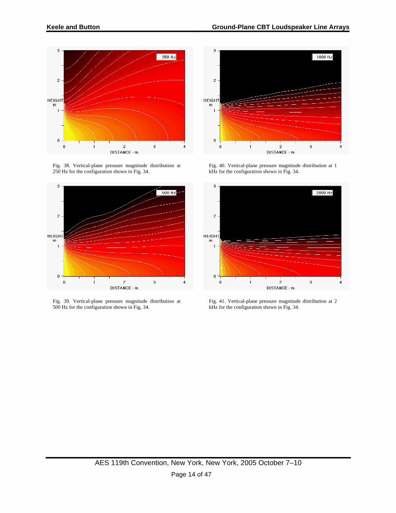
Fig. 38. Vertical-plane pressure magnitude distribution at 250 Hz for the configuration shown in Fig. 34.
Fig. 39. Vertical-plane pressure magnitude distribution at 500 Hz for the configuration shown in Fig. 34.
Fig. 40. Vertical-plane pressure magnitude distribution at 1 kHz for the configuration shown in Fig. 34.
Fig. 41. Vertical-plane pressure magnitude distribution at 2 kHz for the configuration shown in Fig. 34.
Keele and Button Ground-Plane CBT Loudspeaker Line Arrays
AES 119th Convention, New York, New York, 2005 October 7–10 Page 15 of 47
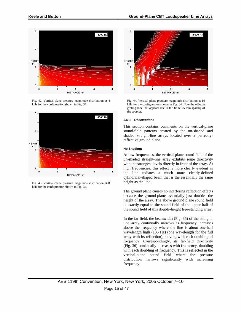
Fig. 42. Vertical-plane pressure magnitude distribution at 4 kHz for the configuration shown in Fig. 34.
Fig. 43. Vertical-plane pressure magnitude distribution at 8 kHz for the configuration shown in Fig. 34.
Fig. 44. Vertical-plane pressure magnitude distribution at 16 kHz for the configuration shown in Fig. 34. Note the off-axis grating lobe that appears due to the finite 25 mm spacing of the sources.
3.5.3. Observations
This section contains comments on the vertical-plane sound-field patterns created by the un-shaded and shaded straight-line arrays located over a perfectly-reflective ground plane.
No Shading:
At low frequencies, the vertical-plane sound field of the un-shaded straight-line array exhibits some directivity with the strongest levels directly in front of the array. At high frequencies, this effect is more clearly evident as the line radiates a much more clearly-defined cylindrical-shaped beam that is the essentially the same height as the line.
The ground plane causes no interfering reflection effects because the ground-plane essentially just doubles the height of the array. The above ground plane sound field is exactly equal to the sound field of the upper half of the sound field of this double-height free-standing array.
In the far field, the beamwidth (Fig. 35) of the straight-line array continually narrows as frequency increases above the frequency where the line is about one-half wavelength high (135 Hz) (one wavelength for the full array with its reflection), halving with each doubling of frequency. Correspondingly, its far-field directivity (Fig. 36) continually increases with frequency, doubling with each doubling of frequency. This is reflected in the vertical-plane sound field where the pressure distribution narrows significantly with increasing frequency.
Keele and Button Ground-Plane CBT Loudspeaker Line Arrays
AES 119th Convention, New York, New York, 2005 October 7–10 Page 16 of 47
What is quite significant in most of the figures is the rapid variation and undulation of sound pressure with position both in front of and above the array, and the out-of-beam lobing and fingering. The fine detail of these effects changes dramatically with frequency. Note that even close to the array, the sound field changes quite significantly with frequency. Note also that the lobing and rapid pressure undulations with position are not due to the ground-plane reflection but are inherent in the radiation pattern of any un-shaded straight-line array.
At 16 kHz (Fig.33), an off-axis grating lobe appears due to the finite 25 mm spacing of the sources.
With Hann Shading:
With Hann shading of the array’s sources (Figs. 9 and 34), the vertical-plane radiation of the array is considerably more well behaved. Completely missing is the rapid variation and undulation of sound pressure and the out-of-beam lobing and fingering noted in the sound-field of the un-shaded array. Even with shading however, the vertical sound-field still changes significantly with frequency and narrows as frequency increases.
Note that the shading has essentially no effect on the grating lobe seen in the 16 kHz distributions (Figs. 33 and 44).
3.6. Circular-Arc Line Source
In this section, the straight-line array of the previous section is physically curved into a circular arc and then re-analyzed with and without shading. Rather than using Hann shading that operates best for the straight-line arrays, a Legendre shading is used which works best for circular-arc arrays (Fig.9).
A 45º circular-arc curved-line array of height 1.25 m (50”) is located with its bottom resting on a perfectly-reflective ground plane. The array is composed of 50 point sources spaced approximately 27.9 mm (1.1”) apart..
3.6.1. No Shading
All the array’s sources are on with equal and in-phase levels. This situation is illustrated in the next figure.
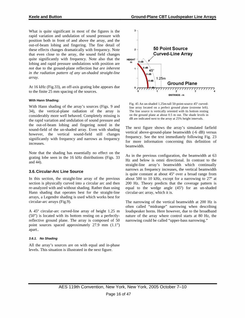
Fig. 45 An un-shaded 1.25m-tall 50-point-source 45º curved-line array located on a perfect ground plane (extreme left). The line source is vertically oriented with its bottom resting on the ground plane at about 0.5 m out. The shade levels in dB are indicated next to the array at 25% height intervals.
The next figure shows the array’s simulated farfield vertical above-ground-plane beamwidth (-6 dB) versus frequency. See the text immediately following Fig. 23 for more information concerning this definition of beamwidth.
As in the previous configuration, the beamwidth at 63 Hz and below is omni directional. In contrast to the straight-line array’s beamwidth which continually narrows as frequency increases, the vertical beamwidth is quite constant at about 45º over a broad range from about 500 to 10 kHz, except for a narrowing to 27º at 200 Hz. Theory predicts that the coverage pattern is equal to the wedge angle (45º) for an un-shaded circular-arc array, which it is.
The narrowing of the vertical beamwidth at 200 Hz is often called “midrange” narrowing when describing loudspeaker horns. Here however, due to the broadband nature of the array where control starts at 80 Hz, the narrowing could be called “upper-bass narrowing.”
Keele and Button Ground-Plane CBT Loudspeaker Line Arrays
AES 119th Convention, New York, New York, 2005 October 7–10 Page 17 of 47
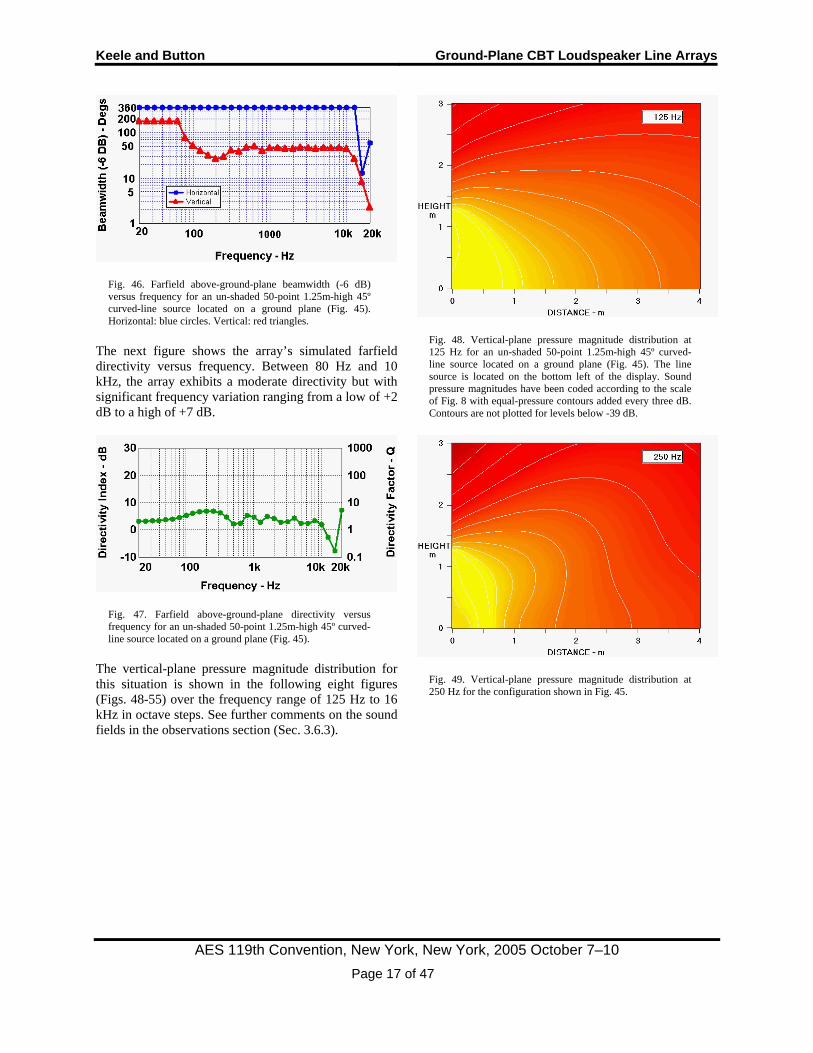
Fig. 46. Farfield above-ground-plane beamwidth (-6 dB) versus frequency for an un-shaded 50-point 1.25m-high 45º curved-line source located on a ground plane (Fig. 45). Horizontal: blue circles. Vertical: red triangles.
The next figure shows the array’s simulated farfield directivity versus frequency. Between 80 Hz and 10 kHz, the array exhibits a moderate directivity but with significant frequency variation ranging from a low of +2 dB to a high of +7 dB.
Fig. 47. Farfield above-ground-plane directivity versus frequency for an un-shaded 50-point 1.25m-high 45º curved-line source located on a ground plane (Fig. 45).
The vertical-plane pressure magnitude distribution for this situation is shown in the following eight figures (Figs. 48-55) over the frequency range of 125 Hz to 16 kHz in octave steps. See further comments on the sound fields in the observations section (Sec. 3.6.3).
Fig. 48. Vertical-plane pressure magnitude distribution at 125 Hz for an un-shaded 50-point 1.25m-high 45º curved-line source located on a ground plane (Fig. 45). The line source is located on the bottom left of the display. Sound pressure magnitudes have been coded according to the scale of Fig. 8 with equal-pressure contours added every three dB. Contours are not plotted for levels below -39 dB.
Fig. 49. Vertical-plane pressure magnitude distribution at 250 Hz for the configuration shown in Fig. 45.
Keele and Button Ground-Plane CBT Loudspeaker Line Arrays
AES 119th Convention, New York, New York, 2005 October 7–10 Page 18 of 47
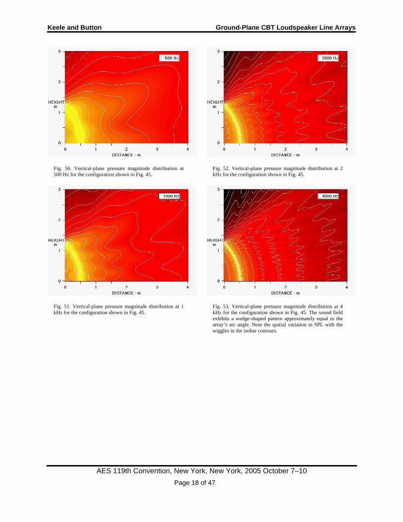
Fig. 50. Vertical-plane pressure magnitude distribution at 500 Hz for the configuration shown in Fig. 45.
Fig. 51. Vertical-plane pressure magnitude distribution at 1 kHz for the configuration shown in Fig. 45.
Fig. 52. Vertical-plane pressure magnitude distribution at 2 kHz for the configuration shown in Fig. 45.
Fig. 53. Vertical-plane pressure magnitude distribution at 4 kHz for the configuration shown in Fig. 45. The sound field exhibits a wedge-shaped pattern approximately equal to the array’s arc angle. Note the spatial variation in SPL with the wiggles in the isobar contours.
Keele and Button Ground-Plane CBT Loudspeaker Line Arrays
AES 119th Convention, New York, New York, 2005 October 7–10 Page 19 of 47
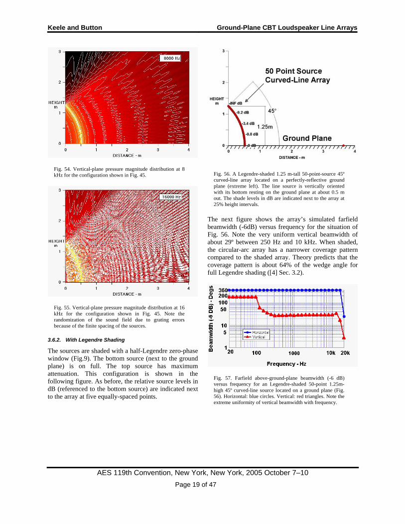
Fig. 54. Vertical-plane pressure magnitude distribution at 8 kHz for the configuration shown in Fig. 45.
Fig. 55. Vertical-plane pressure magnitude distribution at 16 kHz for the configuration shown in Fig. 45. Note the randomization of the sound field due to grating errors because of the finite spacing of the sources.
3.6.2. With Legendre Shading
The sources are shaded with a half-Legendre zero-phase window (Fig.9). The bottom source (next to the ground plane) is on full. The top source has maximum attenuation. This configuration is shown in the following figure. As before, the relative source levels in dB (referenced to the bottom source) are indicated next to the array at five equally-spaced points.
Fig. 56. A Legendre-shaded 1.25 m-tall 50-point-source 45º curved-line array located on a perfectly-reflective ground plane (extreme left). The line source is vertically oriented with its bottom resting on the ground plane at about 0.5 m out. The shade levels in dB are indicated next to the array at 25% height intervals.
The next figure shows the array’s simulated farfield beamwidth (-6dB) versus frequency for the situation of Fig. 56. Note the very uniform vertical beamwidth of about 29º between 250 Hz and 10 kHz. When shaded, the circular-arc array has a narrower coverage pattern compared to the shaded array. Theory predicts that the coverage pattern is about 64% of the wedge angle for full Legendre shading ([4] Sec. 3.2).
Fig. 57. Farfield above-ground-plane beamwidth (-6 dB) versus frequency for an Legendre-shaded 50-point 1.25m-high 45º curved-line source located on a ground plane (Fig. 56). Horizontal: blue circles. Vertical: red triangles. Note the extreme uniformity of vertical beamwidth with frequency.
Keele and Button Ground-Plane CBT Loudspeaker Line Arrays
AES 119th Convention, New York, New York, 2005 October 7–10 Page 20 of 47
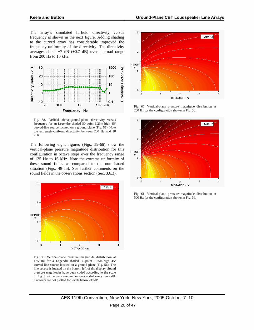
The array’s simulated farfield directivity versus frequency is shown in the next figure. Adding shading to the curved array has considerable improved the frequency uniformity of the directivity. The directivity averages about +7 dB (±0.7 dB) over a broad range from 200 Hz to 10 kHz.
Fig. 58. Farfield above-ground-plane directivity versus frequency for an Legendre-shaded 50-point 1.25m-high 45º curved-line source located on a ground plane (Fig. 56). Note the extremely-uniform directivity between 200 Hz and 10 kHz.
The following eight figures (Figs. 59-66) show the vertical-plane pressure magnitude distribution for this configuration in octave steps over the frequency range of 125 Hz to 16 kHz. Note the extreme uniformity of these sound fields as compared to the non-shaded situation (Figs. 48-55). See further comments on the sound fields in the observations section (Sec. 3.6.3).
Fig. 59. Vertical-plane pressure magnitude distribution at 125 Hz for a Legendre-shaded 50-point 1.25m-high 45º curved-line source located on a ground plane (Fig. 56). The line source is located on the bottom left of the display. Sound pressure magnitudes have been coded according to the scale of Fig. 8 with equal-pressure contours added every three dB. Contours are not plotted for levels below -39 dB.
Fig. 60. Vertical-plane pressure magnitude distribution at 250 Hz for the configuration shown in Fig. 56.
Fig. 61. Vertical-plane pressure magnitude distribution at 500 Hz for the configuration shown in Fig. 56.
Keele and Button Ground-Plane CBT Loudspeaker Line Arrays
AES 119th Convention, New York, New York, 2005 October 7–10 Page 21 of 47
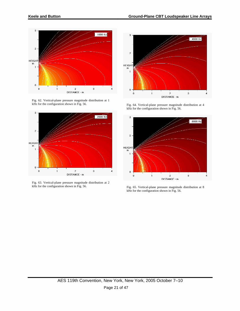
Fig. 62. Vertical-plane pressure magnitude distribution at 1 kHz for the configuration shown in Fig. 56.
Fig. 63. Vertical-plane pressure magnitude distribution at 2 kHz for the configuration shown in Fig. 56.
Fig. 64. Vertical-plane pressure magnitude distribution at 4 kHz for the configuration shown in Fig. 56.
Fig. 65. Vertical-plane pressure magnitude distribution at 8 kHz for the configuration shown in Fig. 56.
Keele and Button Ground-Plane CBT Loudspeaker Line Arrays
AES 119th Convention, New York, New York, 2005 October 7–10 Page 22 of 47
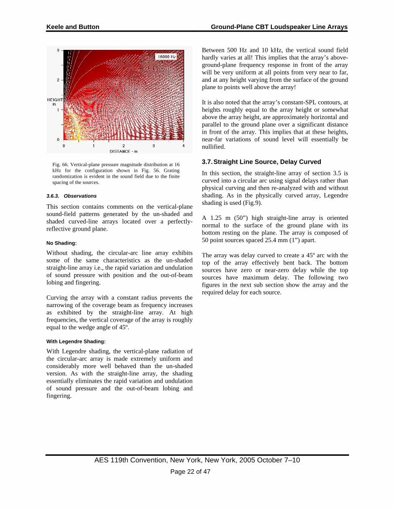
Fig. 66. Vertical-plane pressure magnitude distribution at 16 kHz for the configuration shown in Fig. 56. Grating randomization is evident in the sound field due to the finite spacing of the sources.
3.6.3. Observations
This section contains comments on the vertical-plane sound-field patterns generated by the un-shaded and shaded curved-line arrays located over a perfectly-reflective ground plane.
No Shading:
Without shading, the circular-arc line array exhibits some of the same characteristics as the un-shaded straight-line array i.e., the rapid variation and undulation of sound pressure with position and the out-of-beam lobing and fingering.
Curving the array with a constant radius prevents the narrowing of the coverage beam as frequency increases as exhibited by the straight-line array. At high frequencies, the vertical coverage of the array is roughly equal to the wedge angle of 45º.
With Legendre Shading:
With Legendre shading, the vertical-plane radiation of the circular-arc array is made extremely uniform and considerably more well behaved than the un-shaded version. As with the straight-line array, the shading essentially eliminates the rapid variation and undulation of sound pressure and the out-of-beam lobing and fingering.
Between 500 Hz and 10 kHz, the vertical sound field hardly varies at all! This implies that the array’s above-ground-plane frequency response in front of the array will be very uniform at all points from very near to far, and at any height varying from the surface of the ground plane to points well above the array!
It is also noted that the array’s constant-SPL contours, at heights roughly equal to the array height or somewhat above the array height, are approximately horizontal and parallel to the ground plane over a significant distance in front of the array. This implies that at these heights, near-far variations of sound level will essentially be nullified.
3.7. Straight Line Source, Delay Curved
In this section, the straight-line array of section 3.5 is curved into a circular arc using signal delays rather than physical curving and then re-analyzed with and without shading. As in the physically curved array, Legendre shading is used (Fig.9).
A 1.25 m (50”) high straight-line array is oriented normal to the surface of the ground plane with its bottom resting on the plane. The array is composed of 50 point sources spaced 25.4 mm (1”) apart.
The array was delay curved to create a 45º arc with the top of the array effectively bent back. The bottom sources have zero or near-zero delay while the top sources have maximum delay. The following two figures in the next sub section show the array and the required delay for each source.
Keele and Button Ground-Plane CBT Loudspeaker Line Arrays
AES 119th Convention, New York, New York, 2005 October 7–10 Page 23 of 47
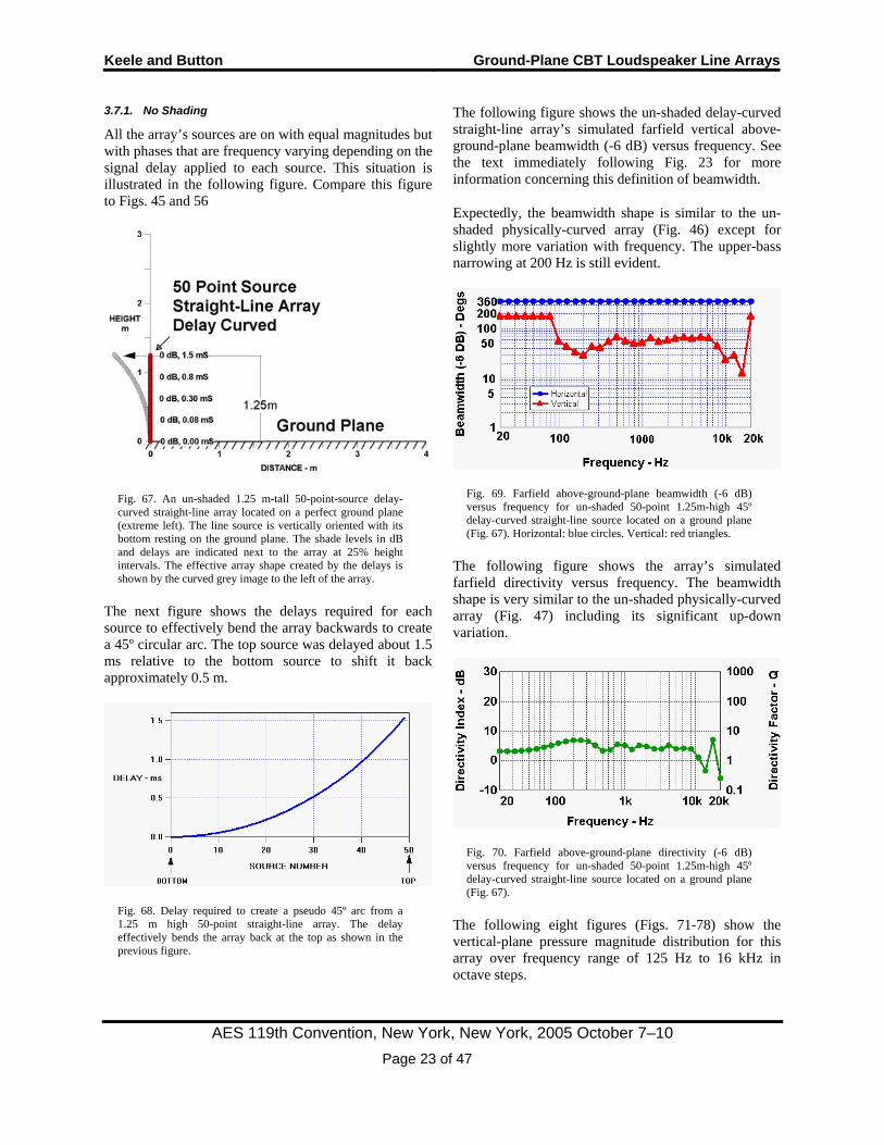
3.7.1. No Shading
All the array’s sources are on with equal magnitudes but with phases that are frequency varying depending on the signal delay applied to each source. This situation is illustrated in the following figure. Compare this figure to Figs. 45 and 56
Fig. 67. An un-shaded 1.25 m-tall 50-point-source delay-curved straight-line array located on a perfect ground plane (extreme left). The line source is vertically oriented with its bottom resting on the ground plane. The shade levels in dB and delays are indicated next to the array at 25% height intervals. The effective array shape created by the delays is shown by the curved grey image to the left of the array.
The next figure shows the delays required for each source to effectively bend the array backwards to create a 45º circular arc. The top source was delayed about 1.5 ms relative to the bottom source to shift it back approximately 0.5 m.
Fig. 68. Delay required to create a pseudo 45º arc from a 1.25 m high 50-point straight-line array. The delay effectively bends the array back at the top as shown in the previous figure.
The following figure shows the un-shaded delay-curved straight-line array’s simulated farfield vertical above-ground-plane beamwidth (-6 dB) versus frequency. See the text immediately following Fig. 23 for more information concerning this definition of beamwidth.
Expectedly, the beamwidth shape is similar to the un-shaded physically-curved array (Fig. 46) except for slightly more variation with frequency. The upper-bass narrowing at 200 Hz is still evident.
Fig. 69. Farfield above-ground-plane beamwidth (-6 dB) versus frequency for un-shaded 50-point 1.25m-high 45º delay-curved straight-line source located on a ground plane (Fig. 67). Horizontal: blue circles. Vertical: red triangles.
The following figure shows the array’s simulated farfield directivity versus frequency. The beamwidth shape is very similar to the un-shaded physically-curved array (Fig. 47) including its significant up-down variation.
Fig. 70. Farfield above-ground-plane directivity (-6 dB) versus frequency for un-shaded 50-point 1.25m-high 45º delay-curved straight-line source located on a ground plane (Fig. 67).
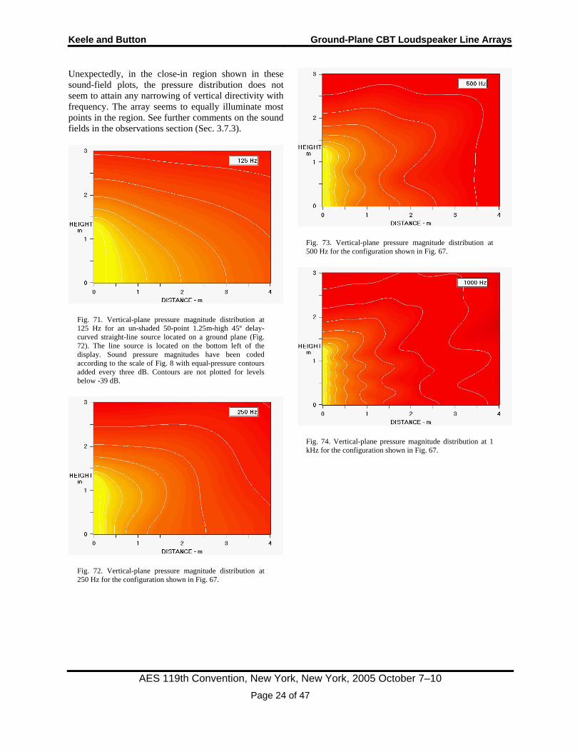
The following eight figures (Figs. 71-78) show the vertical-plane pressure magnitude distribution for this array over frequency range of 125 Hz to 16 kHz in octave steps.
Keele and Button Ground-Plane CBT Loudspeaker Line Arrays
AES 119th Convention, New York, New York, 2005 October 7–10 Page 24 of 47
Unexpectedly, in the close-in region shown in these sound-field plots, the pressure distribution does not seem to attain any narrowing of vertical directivity with frequency. The array seems to equally illuminate most points in the region. See further comments on the sound fields in the observations section (Sec. 3.7.3).
Fig. 71. Vertical-plane pressure magnitude distribution at 125 Hz for an un-shaded 50-point 1.25m-high 45º delay-curved straight-line source located on a ground plane (Fig. 72). The line source is located on the bottom left of the display. Sound pressure magnitudes have been coded according to the scale of Fig. 8 with equal-pressure contours added every three dB. Contours are not plotted for levels below -39 dB.
Fig. 72. Vertical-plane pressure magnitude distribution at 250 Hz for the configuration shown in Fig. 67.
Fig. 73. Vertical-plane pressure magnitude distribution at 500 Hz for the configuration shown in Fig. 67.
Fig. 74. Vertical-plane pressure magnitude distribution at 1 kHz for the configuration shown in Fig. 67.
Keele and Button Ground-Plane CBT Loudspeaker Line Arrays
AES 119th Convention, New York, New York, 2005 October 7–10 Page 25 of 47
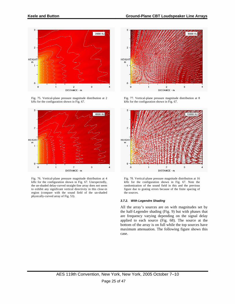
Fig. 75. Vertical-plane pressure magnitude distribution at 2 kHz for the configuration shown in Fig. 67.
Fig. 76. Vertical-plane pressure magnitude distribution at 4 kHz for the configuration shown in Fig. 67. Unexpectedly, the un-shaded delay-curved straight-line array does not seem to exhibit any significant vertical directivity in this close-in region (compare with the sound field of the un-shaded physically-curved array of Fig. 53).
Fig. 77. Vertical-plane pressure magnitude distribution at 8 kHz for the configuration shown in Fig. 67.
Fig. 78. Vertical-plane pressure magnitude distribution at 16 kHz for the configuration shown in Fig. 67. Note the randomization of the sound field in this and the previous figure due to grating errors because of the finite spacing of the sources.
3.7.2. With Legendre Shading
All the array’s sources are on with magnitudes set by the half-Legendre shading (Fig. 9) but with phases that are frequency varying depending on the signal delay applied to each source (Fig. 68). The source at the bottom of the array is on full while the top sources have maximum attenuation. The following figure shows this case.
Keele and Button Ground-Plane CBT Loudspeaker Line Arrays
AES 119th Convention, New York, New York, 2005 October 7–10 Page 26 of 47
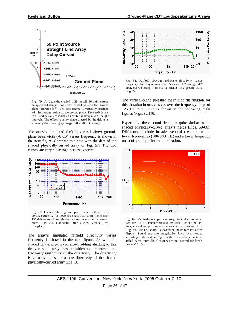
Fig. 79. A Legendre-shaded 1.25 m-tall 50-point-source delay-curved straight-line array located on a perfect ground plane (extreme left). The line source is vertically oriented with its bottom resting on the ground plane. The shade levels in dB and delays are indicated next to the array at 25% height intervals. The effective array shape created by the delays is shown by the curved grey image to the left of the array.
The array’s simulated farfield vertical above-ground-plane beamwidth (-6 dB) versus frequency is shown in the next figure. Compare this data with the data of the shaded physically-curved array of Fig. 57. The two curves are very close together, as expected.
Fig. 80. Farfield above-ground-plane beamwidth (-6 dB) versus frequency for Legendre-shaded 50-point 1.25m-high 45º delay-curved straight-line source located on a ground plane (Fig. 79). Horizontal: blue circles. Vertical: red triangles.
The array’s simulated farfield directivity versus frequency is shown in the next figure. As with the shaded physically-curved array, adding shading to this delay-curved array has considerable improved the frequency uniformity of the directivity. The directivity is virtually the same as the directivity of the shaded physically-curved array (Fig. 58).
Fig. 81. Farfield above-ground-plane directivity versus frequency for Legendre-shaded 50-point 1.25m-high 45º delay-curved straight-line source located on a ground plane (Fig. 79).
The vertical-plane pressure magnitude distribution for this situation in octave steps over the frequency range of 125 Hz to 16 kHz is shown in the following eight figures (Figs. 82-89).
Expectedly, these sound fields are quite similar to the shaded physically-curved array’s fields (Figs. 59-66). Differences include broader vertical coverage at the lower frequencies (500-2000 Hz) and a lower frequency onset of grating-effect randomization.
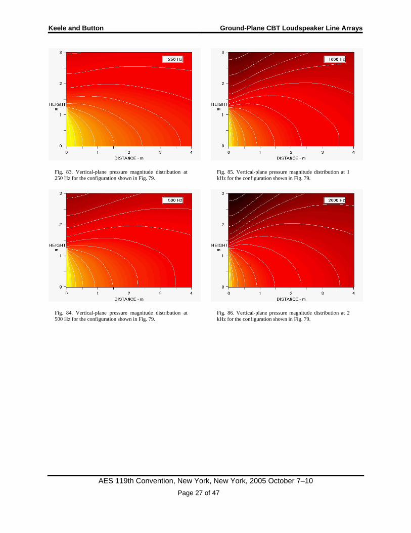
Fig. 82. Vertical-plane pressure magnitude distribution at 125 Hz for a Legendre-shaded 50-point 1.25m-high 45º delay-curved straight-line source located on a ground plane (Fig. 79). The line source is located on the bottom left of the display. Sound pressure magnitudes have been coded according to the scale of Fig. 8 with equal-pressure contours added every three dB. Contours are not plotted for levels below -39 dB.
Keele and Button Ground-Plane CBT Loudspeaker Line Arrays
AES 119th Convention, New York, New York, 2005 October 7–10 Page 27 of 47
Fig. 83. Vertical-plane pressure magnitude distribution at 250 Hz for the configuration shown in Fig. 79.
Fig. 84. Vertical-plane pressure magnitude distribution at 500 Hz for the configuration shown in Fig. 79.
Fig. 85. Vertical-plane pressure magnitude distribution at 1 kHz for the configuration shown in Fig. 79.
Fig. 86. Vertical-plane pressure magnitude distribution at 2 kHz for the configuration shown in Fig. 79.
Keele and Button Ground-Plane CBT Loudspeaker Line Arrays
AES 119th Convention, New York, New York, 2005 October 7–10 Page 28 of 47
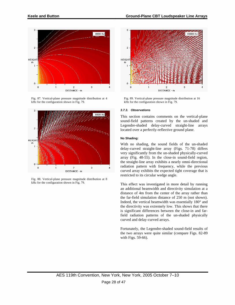
Fig. 87. Vertical-plane pressure magnitude distribution at 4 kHz for the configuration shown in Fig. 79.
Fig. 88. Vertical-plane pressure magnitude distribution at 8 kHz for the configuration shown in Fig. 79.
Fig. 89. Vertical-plane pressure magnitude distribution at 16 kHz for the configuration shown in Fig. 79.
3.7.3. Observations
This section contains comments on the vertical-plane sound-field patterns created by the un-shaded and Legendre-shaded delay-curved straight-line arrays located over a perfectly-reflective ground plane.
No Shading:
With no shading, the sound fields of the un-shaded delay-curved straight-line array (Figs. 71-78) differs very significantly from the un-shaded physically-curved array (Fig. 48-55). In the close-in sound-field region, the straight-line array exhibits a nearly omni-directional radiation pattern with frequency, while the previous curved array exhibits the expected tight coverage that is restricted to its circular wedge angle.
This effect was investigated in more detail by running an additional beamwidth and directivity simulation at a distance of 4m from the center of the array rather than the far-field simulation distance of 250 m (not shown). Indeed, the vertical beamwidth was essentially 180° and the directivity was extremely low. This shows that there is significant differences between the close-in and far-field radiation patterns of the un-shaded physically curved and delay-curved arrays.
Fortunately, the Legendre-shaded sound-field results of the two arrays were quite similar (compare Figs. 82-89 with Figs. 59-66).
Keele and Button Ground-Plane CBT Loudspeaker Line Arrays
AES 119th Convention, New York, New York, 2005 October 7–10 Page 29 of 47
With Legendre Shading:
Expectedly (and fortunately), the sound fields of the shaded delay-curved straight-line array and the shaded physically-curved circular-arc array were quite similar.
Differences included a somewhat broader vertical coverage at lower frequencies (500 Hz to 2 kHz), and a grating-effect randomization that occurred about an octave lower for the straight-line array. The former difference is due to the extreme off-axis differences between the delays due to the physical curving and delay curving. At extreme off-axis observation points, the delay curving significantly distorts the circular shape of the array.
4. FREQUENCY-RESPONSE MEASUREMENTS
4.1. Description
Measurements were made of a conventional powered two-way compact monitor and two experimental line arrays. All systems were measured over a perfectly reflective ground plane (a tile floor located in a large warehouse space). The center fronts of all three systems were located at the origin of the measurement region at a distance of 0.0 m. Note that this is in contrast with the simulated sound fields of the previous section which had the curved array shifted out so that its front was at 0.5 m.
The above-ground-plane sound field of each of these systems was investigated by measuring a number of frequency responses in-front-of and to-the-side of the speakers.
4.1.1. Vertical-Plane Sound Field Samples
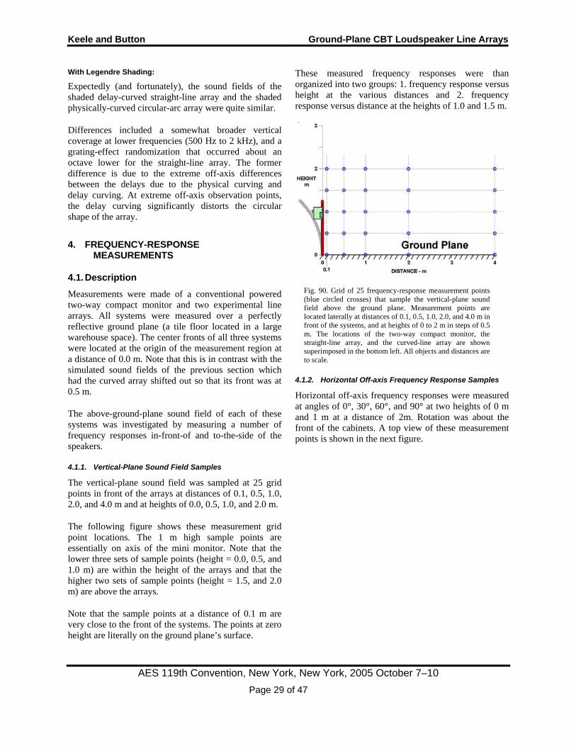
The vertical-plane sound field was sampled at 25 grid points in front of the arrays at distances of 0.1, 0.5, 1.0, 2.0, and 4.0 m and at heights of 0.0, 0.5, 1.0, and 2.0 m.
The following figure shows these measurement grid point locations. The 1 m high sample points are essentially on axis of the mini monitor. Note that the lower three sets of sample points (height = 0.0, 0.5, and 1.0 m) are within the height of the arrays and that the higher two sets of sample points (height = 1.5, and 2.0 m) are above the arrays.
Note that the sample points at a distance of 0.1 m are very close to the front of the systems. The points at zero height are literally on the ground plane’s surface.
These measured frequency responses were than organized into two groups: 1. frequency response versus height at the various distances and 2. frequency response versus distance at the heights of 1.0 and 1.5 m.
Fig. 90. Grid of 25 frequency-response measurement points (blue circled crosses) that sample the vertical-plane sound field above the ground plane. Measurement points are located laterally at distances of 0.1, 0.5, 1.0, 2.0, and 4.0 m in front of the systems, and at heights of 0 to 2 m in steps of 0.5 m. The locations of the two-way compact monitor, the straight-line array, and the curved-line array are shown superimposed in the bottom left. All objects and distances are to scale.
4.1.2. Horizontal Off-axis Frequency Response SamplesT
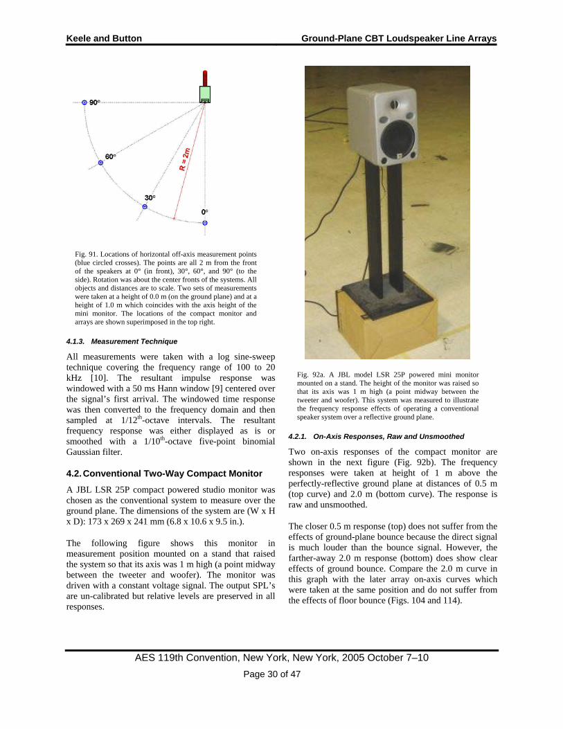
Horizontal off-axis frequency responses were measured at angles of 0°, 30°, 60°, and 90° at two heights of 0 m and 1 m at a distance of 2m. Rotation was about the front of the cabinets. A top view of these measurement points is shown in the next figure.
Keele and Button Ground-Plane CBT Loudspeaker Line Arrays
AES 119th Convention, New York, New York, 2005 October 7–10 Page 30 of 47
Fig. 91. Locations of horizontal off-axis measurement points (blue circled crosses). The points are all 2 m from the front of the speakers at 0° (in front), 30°, 60°, and 90° (to the side). Rotation was about the center fronts of the systems. All objects and distances are to scale. Two sets of measurements were taken at a height of 0.0 m (on the ground plane) and at a height of 1.0 m which coincides with the axis height of the mini monitor. The locations of the compact monitor and arrays are shown superimposed in the top right.
4.1.3. Measurement Technique
All measurements were taken with a log sine-sweep technique covering the frequency range of 100 to 20 kHz [10]. The resultant impulse response was windowed with a 50 ms Hann window [9] centered over the signal’s first arrival. The windowed time response was then converted to the frequency domain and then sampled at 1/12P
thP-octave intervals. The resultant
frequency response was either displayed as is or smoothed with a 1/10P
thP-octave five-point binomial
Gaussian filter.
4.2. Conventional Two-Way Compact Monitor
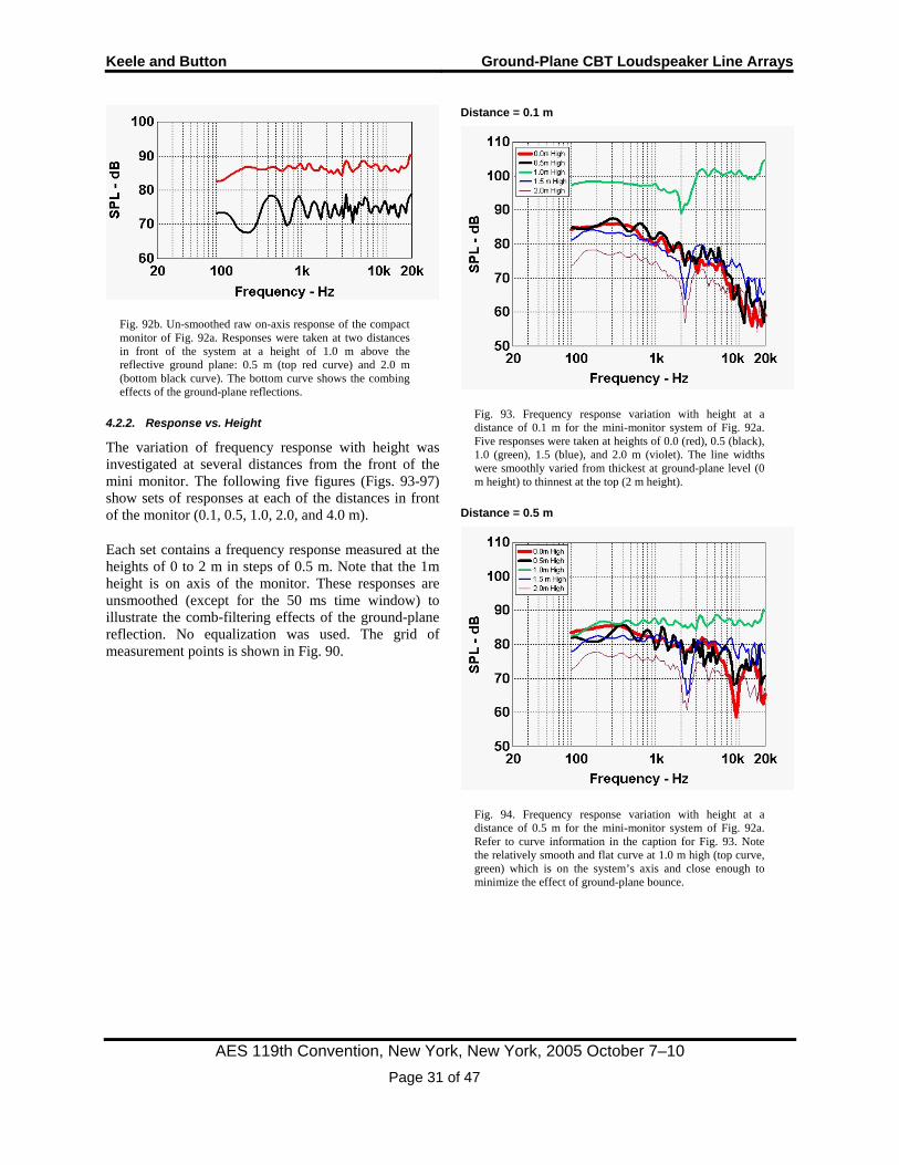
A JBL LSR 25P compact powered studio monitor was chosen as the conventional system to measure over the ground plane. The dimensions of the system are (W x H x D): 173 x 269 x 241 mm (6.8 x 10.6 x 9.5 in.).
The following figure shows this monitor in measurement position mounted on a stand that raised the system so that its axis was 1 m high (a point midway between the tweeter and woofer). The monitor was driven with a constant voltage signal. The output SPL’s are un-calibrated but relative levels are preserved in all responses.
Fig. 92a. A JBL model LSR 25P powered mini monitor mounted on a stand. The height of the monitor was raised so that its axis was 1 m high (a point midway between the tweeter and woofer). This system was measured to illustrate the frequency response effects of operating a conventional speaker system over a reflective ground plane.
4.2.1. On-Axis Responses, Raw and Unsmoothed
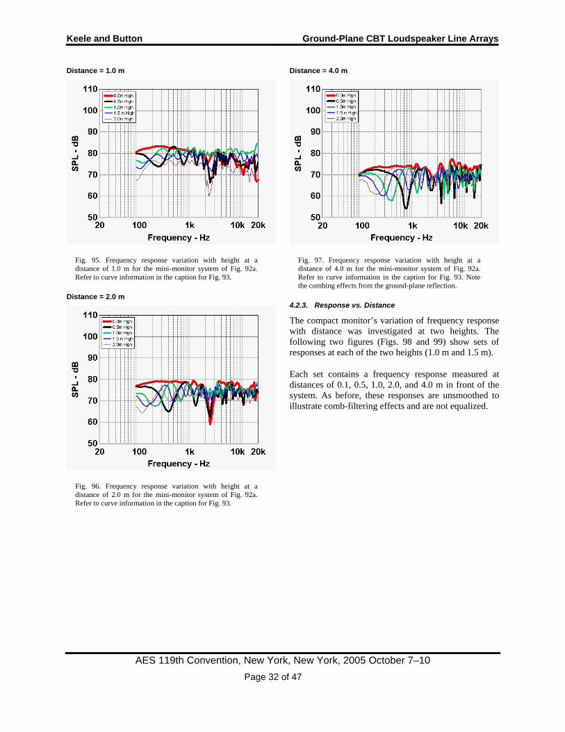
Two on-axis responses of the compact monitor are shown in the next figure (Fig. 92b). The frequency responses were taken at height of 1 m above the perfectly-reflective ground plane at distances of 0.5 m (top curve) and 2.0 m (bottom curve). The response is raw and unsmoothed.
The closer 0.5 m response (top) does not suffer from the effects of ground-plane bounce because the direct signal is much louder than the bounce signal. However, the farther-away 2.0 m response (bottom) does show clear effects of ground bounce. Compare the 2.0 m curve in this graph with the later array on-axis curves which were taken at the same position and do not suffer from the effects of floor bounce (Figs. 104 and 114).
Keele and Button Ground-Plane CBT Loudspeaker Line Arrays
AES 119th Convention, New York, New York, 2005 October 7–10 Page 31 of 47
Fig. 92b. Un-smoothed raw on-axis response of the compact monitor of Fig. 92a. Responses were taken at two distances in front of the system at a height of 1.0 m above the reflective ground plane: 0.5 m (top red curve) and 2.0 m (bottom black curve). The bottom curve shows the combing effects of the ground-plane reflections.
4.2.2. Response vs. Height
The variation of frequency response with height was investigated at several distances from the front of the mini monitor. The following five figures (Figs. 93-97) show sets of responses at each of the distances in front of the monitor (0.1, 0.5, 1.0, 2.0, and 4.0 m).
Each set contains a frequency response measured at the heights of 0 to 2 m in steps of 0.5 m. Note that the 1m height is on axis of the monitor. These responses are unsmoothed (except for the 50 ms time window) to illustrate the comb-filtering effects of the ground-plane reflection. No equalization was used. The grid of measurement points is shown in Fig. 90.
Distance = 0.1 m
Fig. 93. Frequency response variation with height at a distance of 0.1 m for the mini-monitor system of Fig. 92a. Five responses were taken at heights of 0.0 (red), 0.5 (black), 1.0 (green), 1.5 (blue), and 2.0 m (violet). The line widths were smoothly varied from thickest at ground-plane level (0 m height) to thinnest at the top (2 m height).
Distance = 0.5 m
Fig. 94. Frequency response variation with height at a distance of 0.5 m for the mini-monitor system of Fig. 92a. Refer to curve information in the caption for Fig. 93. Note the relatively smooth and flat curve at 1.0 m high (top curve, green) which is on the system’s axis and close enough to minimize the effect of ground-plane bounce.
Keele and Button Ground-Plane CBT Loudspeaker Line Arrays
AES 119th Convention, New York, New York, 2005 October 7–10 Page 32 of 47
Distance = 1.0 m
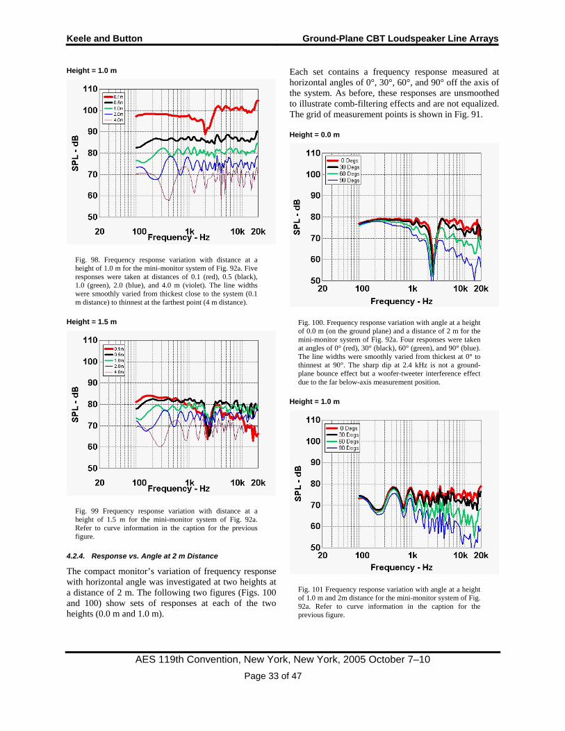
Fig. 95. Frequency response variation with height at a distance of 1.0 m for the mini-monitor system of Fig. 92a. Refer to curve information in the caption for Fig. 93.
Distance = 2.0 m
Fig. 96. Frequency response variation with height at a distance of 2.0 m for the mini-monitor system of Fig. 92a. Refer to curve information in the caption for Fig. 93.
Distance = 4.0 m
Fig. 97. Frequency response variation with height at a distance of 4.0 m for the mini-monitor system of Fig. 92a. Refer to curve information in the caption for Fig. 93. Note the combing effects from the ground-plane reflection.
4.2.3. Response vs. Distance
The compact monitor’s variation of frequency response with distance was investigated at two heights. The following two figures (Figs. 98 and 99) show sets of responses at each of the two heights (1.0 m and 1.5 m).
Each set contains a frequency response measured at distances of 0.1, 0.5, 1.0, 2.0, and 4.0 m in front of the system. As before, these responses are unsmoothed to illustrate comb-filtering effects and are not equalized.
Keele and Button Ground-Plane CBT Loudspeaker Line Arrays
AES 119th Convention, New York, New York, 2005 October 7–10 Page 33 of 47
Height = 1.0 m
Fig. 98. Frequency response variation with distance at a height of 1.0 m for the mini-monitor system of Fig. 92a. Five responses were taken at distances of 0.1 (red), 0.5 (black), 1.0 (green), 2.0 (blue), and 4.0 m (violet). The line widths were smoothly varied from thickest close to the system (0.1 m distance) to thinnest at the farthest point (4 m distance).
Height = 1.5 m
Fig. 99 Frequency response variation with distance at a height of 1.5 m for the mini-monitor system of Fig. 92a. Refer to curve information in the caption for the previous figure.
4.2.4. Response vs. Angle at 2 m Distance
The compact monitor’s variation of frequency response with horizontal angle was investigated at two heights at a distance of 2 m. The following two figures (Figs. 100 and 100) show sets of responses at each of the two heights (0.0 m and 1.0 m).
Each set contains a frequency response measured at horizontal angles of 0°, 30°, 60°, and 90° off the axis of the system. As before, these responses are unsmoothed to illustrate comb-filtering effects and are not equalized. The grid of measurement points is shown in Fig. 91.
Height = 0.0 m
Fig. 100. Frequency response variation with angle at a height of 0.0 m (on the ground plane) and a distance of 2 m for the mini-monitor system of Fig. 92a. Four responses were taken at angles of 0° (red), 30° (black), 60° (green), and 90° (blue). The line widths were smoothly varied from thickest at 0° to thinnest at 90°. The sharp dip at 2.4 kHz is not a ground-plane bounce effect but a woofer-tweeter interference effect due to the far below-axis measurement position.
Height = 1.0 m
Fig. 101 Frequency response variation with angle at a height of 1.0 m and 2m distance for the mini-monitor system of Fig. 92a. Refer to curve information in the caption for the previous figure.
Keele and Button Ground-Plane CBT Loudspeaker Line Arrays
AES 119th Convention, New York, New York, 2005 October 7–10 Page 34 of 47
4.2.5. Observations
This section contains comments on the compact monitor’s measured frequency responses when located over a perfectly-reflective ground plane.
The compact monitor was included in the measurements to show the effect of listening to or measuring a conventional free-standing system when used over a reflective ground plane. The ground plane generates acoustic reflections that interfere with the monitor’s direct sound and are commonly called floor bounce reflections.
Response vs. Height
The frequencies responses taken at various heights at different distances illustrate how the conventional speaker system fares when operated over a reflective ground plane (Figs. 93-97). Note that dramatic change in frequency response with position exhibited by this system, both in smoothness and consistency of response shape. The flattest and smoothest response is only exhibited at a distance of 0.5 m on the system’s axis. The response only gets worse at points closer or farther away or points higher or lower!
Up close (Fig. 93), dramatic changes are evident in both level, smoothness, and response shape. At one meter high, the response is smoothest and flattest but exhibits level changes in the woofer’s and tweeter’s pass-bands. The mic is obviously somewhat closer acoustically to the tweeter than woofer. At points above or below the axis, the test mic is too far off the system’s axis for good response.
At farther distances, the responses are much closer in overall response shape, but suffer from dramatic response undulations due to the ground bounce reflections. At 4 m away (Fig. 97), the composite responses exhibit a response envelope that fits a rather gross 20 dB window. This is in spite of the fact that these locations vertically are within roughly ±15° of the system’s axis.
Response vs. Distance
These curves illustrate how the conventional system’s frequency response changes as a function of distance at a specific height.
At 1 m height (Fig. 98), which is on the system’s axis, the overall curve shape is roughly flat but exhibits dramatic changes in response detail, roughness, and level with increasing distance. The farthest distance (4 m) exhibits the greatest undulations due to ground bounce.
At 1.5 m height (Fig. 99), the response also changes dramatically with distance. This is not altogether surprising, because the vertical off-axis angle varies from nearly 90° up to only 7° above the system’s axis. These angular changes are mixed up with the ground-plane bounce effects. The sharp dips at about 2.4 kHz are not a ground-plane bounce effect but a woofer-tweeter interference effect due to the far above-axis measurement position at close distances.
Response vs. Angle
These curves show how the conventional system’s off axis behavior is effected by the ground plane.
At the height of 0.0 m (which is on the surface of the ground plane) at 2 m distant (Fig. 100), the curves are relatively smooth except for a sharp dip at 2.4 kHz and a high-frequency rolloff as angles increase. As described in the previous sub section, this is not a ground-plane bounce effect but a woofer-tweeter interference effect due to the below-axis measurement position (about 27° below axis).
At the 1 m height (Fig. 101), which is level with the system’s axis, the 2.4 kHz dip is gone, but the curves exhibit upper-mid and high-frequency rolloff coupled with up-down undulations due to reflections from the ground plane.
4.3. Experimental Arrays
Two experimental line arrays were measured: a straight-line array with no shading (equal levels to each driver) and no delays, and a circular-arc 45º curved-line array with Legendre shading and no delays.
Both arrays contained 36 full-range 30 mm (1.181 inch) diameter miniature drivers. The drivers were mounted at a center-to-center spacing of 34.6 mm (1.36 inches). The straight-line array was 1.25 m (49.2 inches) high and the curved-line array was 1.1 m (43.3 inches) high. The drivers were operated in a closed-box enclosure and provided a usable response from 100 Hz to 15 kHz.
Keele and Button Ground-Plane CBT Loudspeaker Line Arrays
AES 119th Convention, New York, New York, 2005 October 7–10 Page 35 of 47
All the drivers were driven individually using three DSP-programmable twelve-channel automotive amplifiers. Individual amplifier drives to each speaker allowed each to be driven with different gains if required. No equalization was used other than the required differences in gain.
An on-axis frequency response point was defined as the response taken at 2 m in front of the system and 1 m high over the reflective ground plane. This on-axis response was used to normalize all the displayed curves. This effectively equalizes the array flat at this location. All curves were smoothed using the technique described in Sec. 4.1.3. Before each set of measurements, the raw un-smoothed on-axis curve is displayed.
4.3.1. Straight-Line Array
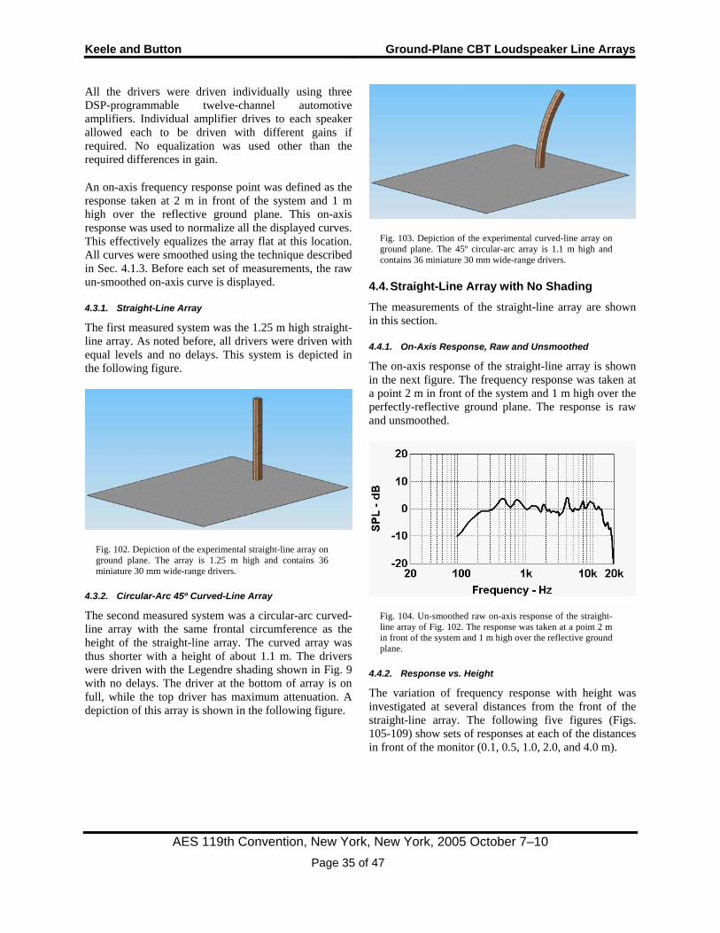
The first measured system was the 1.25 m high straight-line array. As noted before, all drivers were driven with equal levels and no delays. This system is depicted in the following figure.
Fig. 102. Depiction of the experimental straight-line array on ground plane. The array is 1.25 m high and contains 36 miniature 30 mm wide-range drivers.
4.3.2. Circular-Arc 45º Curved-Line Array
The second measured system was a circular-arc curved-line array with the same frontal circumference as the height of the straight-line array. The curved array was thus shorter with a height of about 1.1 m. The drivers were driven with the Legendre shading shown in Fig. 9 with no delays. The driver at the bottom of array is on full, while the top driver has maximum attenuation. A depiction of this array is shown in the following figure.
Fig. 103. Depiction of the experimental curved-line array on ground plane. The 45º circular-arc array is 1.1 m high and contains 36 miniature 30 mm wide-range drivers.
4.4. Straight-Line Array with No Shading
The measurements of the straight-line array are shown in this section.
4.4.1. On-Axis Response, Raw and Unsmoothed
The on-axis response of the straight-line array is shown in the next figure. The frequency response was taken at a point 2 m in front of the system and 1 m high over the perfectly-reflective ground plane. The response is raw and unsmoothed.
Fig. 104. Un-smoothed raw on-axis response of the straight-line array of Fig. 102. The response was taken at a point 2 m in front of the system and 1 m high over the reflective ground plane.
4.4.2. Response vs. Height
The variation of frequency response with height was investigated at several distances from the front of the straight-line array. The following five figures (Figs. 105-109) show sets of responses at each of the distances in front of the monitor (0.1, 0.5, 1.0, 2.0, and 4.0 m).
Keele and Button Ground-Plane CBT Loudspeaker Line Arrays
AES 119th Convention, New York, New York, 2005 October 7–10 Page 36 of 47
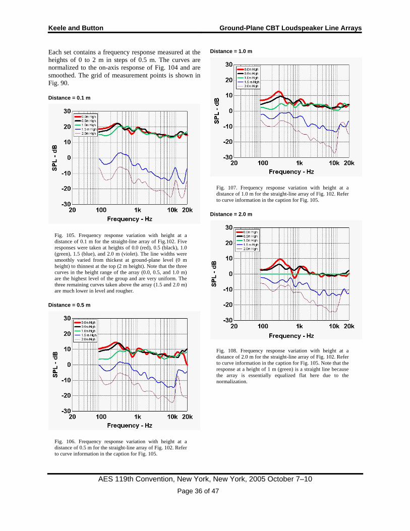
Each set contains a frequency response measured at the heights of 0 to 2 m in steps of 0.5 m. The curves are normalized to the on-axis response of Fig. 104 and are smoothed. The grid of measurement points is shown in Fig. 90.
Distance = 0.1 m
Fig. 105. Frequency response variation with height at a distance of 0.1 m for the straight-line array of Fig.102. Five responses were taken at heights of 0.0 (red), 0.5 (black), 1.0 (green), 1.5 (blue), and 2.0 m (violet). The line widths were smoothly varied from thickest at ground-plane level (0 m height) to thinnest at the top (2 m height). Note that the three curves in the height range of the array (0.0, 0.5, and 1.0 m) are the highest level of the group and are very uniform. The three remaining curves taken above the array (1.5 and 2.0 m) are much lower in level and rougher.
Distance = 0.5 m
Fig. 106. Frequency response variation with height at a distance of 0.5 m for the straight-line array of Fig. 102. Refer to curve information in the caption for Fig. 105.
Distance = 1.0 m
Fig. 107. Frequency response variation with height at a distance of 1.0 m for the straight-line array of Fig. 102. Refer to curve information in the caption for Fig. 105.
Distance = 2.0 m
Fig. 108. Frequency response variation with height at a distance of 2.0 m for the straight-line array of Fig. 102. Refer to curve information in the caption for Fig. 105. Note that the response at a height of 1 m (green) is a straight line because the array is essentially equalized flat here due to the normalization.
Keele and Button Ground-Plane CBT Loudspeaker Line Arrays
AES 119th Convention, New York, New York, 2005 October 7–10 Page 37 of 47
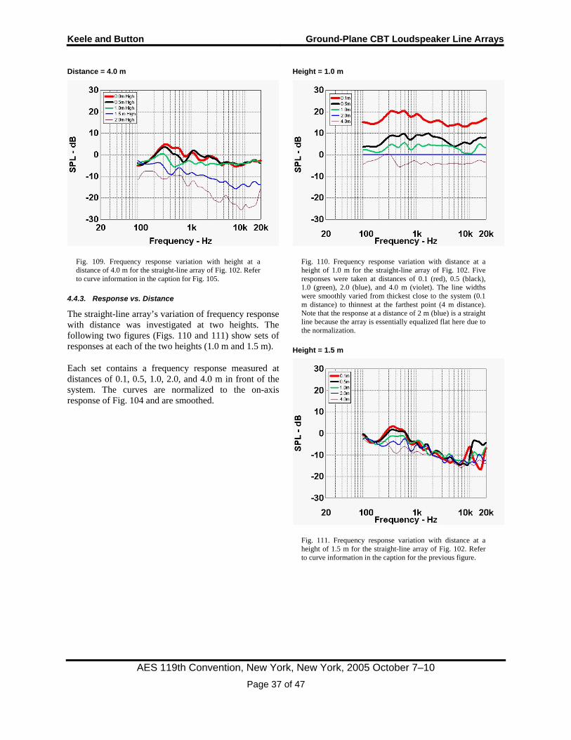
Distance = 4.0 m
Fig. 109. Frequency response variation with height at a distance of 4.0 m for the straight-line array of Fig. 102. Refer to curve information in the caption for Fig. 105.
4.4.3. Response vs. Distance
The straight-line array’s variation of frequency response with distance was investigated at two heights. The following two figures (Figs. 110 and 111) show sets of responses at each of the two heights (1.0 m and 1.5 m).
Each set contains a frequency response measured at distances of 0.1, 0.5, 1.0, 2.0, and 4.0 m in front of the system. The curves are normalized to the on-axis response of Fig. 104 and are smoothed.
Height = 1.0 m
Fig. 110. Frequency response variation with distance at a height of 1.0 m for the straight-line array of Fig. 102. Five responses were taken at distances of 0.1 (red), 0.5 (black), 1.0 (green), 2.0 (blue), and 4.0 m (violet). The line widths were smoothly varied from thickest close to the system (0.1 m distance) to thinnest at the farthest point (4 m distance). Note that the response at a distance of 2 m (blue) is a straight line because the array is essentially equalized flat here due to the normalization.
Height = 1.5 m
Fig. 111. Frequency response variation with distance at a height of 1.5 m for the straight-line array of Fig. 102. Refer to curve information in the caption for the previous figure.
Keele and Button Ground-Plane CBT Loudspeaker Line Arrays
AES 119th Convention, New York, New York, 2005 October 7–10 Page 38 of 47
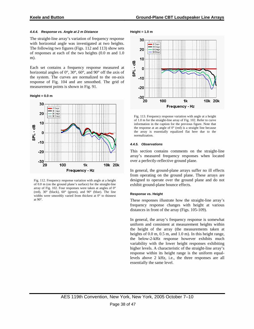
4.4.4. Response vs. Angle at 2 m Distance
The straight-line array’s variation of frequency response with horizontal angle was investigated at two heights. The following two figures (Figs. 112 and 113) show sets of responses at each of the two heights (0.0 m and 1.0 m).
Each set contains a frequency response measured at horizontal angles of 0°, 30°, 60°, and 90° off the axis of the system. The curves are normalized to the on-axis response of Fig. 104 and are smoothed. The grid of measurement points is shown in Fig. 91.
Height = 0.0 m
Fig. 112. Frequency response variation with angle at a height of 0.0 m (on the ground plane’s surface) for the straight-line array of Fig. 102. Four responses were taken at angles of 0° (red), 30° (black), 60° (green), and 90° (blue). The line widths were smoothly varied from thickest at 0° to thinnest at 90°.
Height = 1.0 m
Fig. 113. Frequency response variation with angle at a height of 1.0 m for the straight-line array of Fig. 102. Refer to curve information in the caption for the previous figure. Note that the response at an angle of 0° (red) is a straight line because the array is essentially equalized flat here due to the normalization.
4.4.5. Observations
This section contains comments on the straight-line array’s measured frequency responses when located over a perfectly-reflective ground plane.
In general, the ground-plane arrays suffer no ill effects from operating on the ground plane. These arrays are designed to operate over the ground plane and do not exhibit ground-plane bounce effects.
Response vs. Height
These responses illustrate how the straight-line array’s frequency response changes with height at various distances in front of the array (Figs. 105-109).
In general, the array’s frequency response is somewhat uniform and consistent at measurement heights within the height of the array (the measurements taken at heights of 0.0 m, 0.5 m, and 1.0 m). In this height range, the below-2-kHz response however exhibits much variability with the lower height responses exhibiting higher levels. A characteristic of the straight-line array’s response within its height range is the uniform equal-levels above 2 kHz, i.e., the three responses are all essentially the same level.
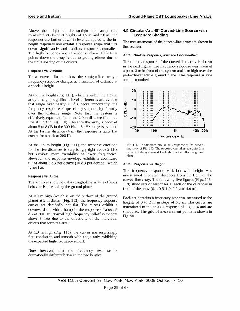
Keele and Button Ground-Plane CBT Loudspeaker Line Arrays
AES 119th Convention, New York, New York, 2005 October 7–10 Page 39 of 47
Above the height of the straight line array (the measurements taken at heights of 1.5 m, and 2.0 m), the responses are farther down in level compared to the in-height responses and exhibit a response shape that tilts down significantly and exhibits response anomalies. The high-frequency rise in response above 10 kHz at points above the array is due to grating effects due to the finite spacing of the drivers.
Response vs. Distance
These curves illustrate how the straight-line array’s frequency response changes as a function of distance at a specific height
At the 1 m height (Fig. 110), which is within the 1.25 m array’s height, significant level differences are evident that range over nearly 25 dB. More importantly, the frequency response shape changes quite significantly over this distance range. Note that the system is effectively equalized flat at the 2.0 m distance (flat blue line at 0 dB in Fig. 110). Closer to the array, a boost of about 5 to 8 dB in the 300 Hz to 3 kHz range is evident. At the farther distance (4 m) the response is quite flat except for a peak at 200 Hz.
At the 1.5 m height (Fig. 111), the response envelope for the five distances is surprisingly tight above 2 kHz but exhibits more variability at lower frequencies. However, the response envelope exhibits a downward tilt of about 3 dB per octave (10 dB per decade), which is not flat.
Response vs. Angle
These curves show how the straight-line array’s off-axis behavior is effected by the ground plane.
At 0.0 m high (which is on the surface of the ground plane) at 2 m distant (Fig. 112), the frequency response curves are decidedly not flat. The curves exhibit a downward tilt with a hump in the response of about 8 dB at 200 Hz. Normal high-frequency rolloff is evident above 5 kHz due to the directivity of the individual drivers that form the array.
At 1.0 m high (Fig. 113), the curves are surprisingly flat, consistent, and smooth with angle only exhibiting the expected high-frequency rolloff.
Note however, that the frequency response is dramatically different between the two heights.
4.5. Circular-Arc 45º Curved-Line Source with Legendre Shading
The measurements of the curved-line array are shown in this section.
4.5.1. On-Axis Response, Raw and Un-Smoothed
The on-axis response of the curved-line array is shown in the next figure. The frequency response was taken at a point 2 m in front of the system and 1 m high over the perfectly-reflective ground plane. The response is raw and unsmoothed.
Fig. 114. Un-smoothed raw on-axis response of the curved-line array of Fig. 103. The response was taken at a point 2 m in front of the system and 1 m high over the reflective ground plane.
4.5.2. Response vs. Height
The frequency response variation with height was investigated at several distances from the front of the curved-line array. The following five figures (Figs. 115-119) show sets of responses at each of the distances in front of the array (0.1, 0.5, 1.0, 2.0, and 4.0 m).
Each set contains a frequency response measured at the heights of 0 to 2 m in steps of 0.5 m. The curves are normalized to the on-axis response of Fig. 114 and are smoothed. The grid of measurement points is shown in Fig. 90.
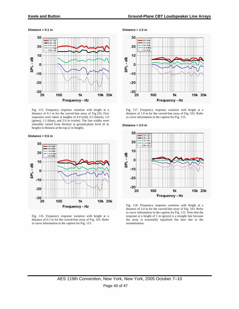
Keele and Button Ground-Plane CBT Loudspeaker Line Arrays
AES 119th Convention, New York, New York, 2005 October 7–10 Page 40 of 47
Distance = 0.1 m
Fig. 115. Frequency response variation with height at a distance of 0.1 m for the curved-line array of Fig.103. Five responses were taken at heights of 0.0 (red), 0.5 (black), 1.0 (green), 1.5 (blue), and 2.0 m (violet). The line widths were smoothly varied from thickest at ground-plane level (0 m height) to thinnest at the top (2 m height).
Distance = 0.5 m
Fig. 116. Frequency response variation with height at a distance of 0.5 m for the curved-line array of Fig. 103. Refer to curve information in the caption for Fig. 115.
Distance = 1.0 m
Fig. 117. Frequency response variation with height at a distance of 1.0 m for the curved-line array of Fig. 103. Refer to curve information in the caption for Fig. 115.
Distance = 2.0 m
Fig. 118. Frequency response variation with height at a distance of 2.0 m for the curved-line array of Fig. 103. Refer to curve information in the caption for Fig. 115. Note that the response at a height of 1 m (green) is a straight line because the array is essentially equalized flat here due to the normalization.
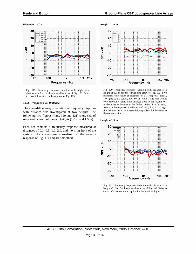
Keele and Button Ground-Plane CBT Loudspeaker Line Arrays
AES 119th Convention, New York, New York, 2005 October 7–10 Page 41 of 47
Distance = 4.0 m
Fig. 119. Frequency response variation with height at a distance of 4.0 m for the curved-line array of Fig. 103. Refer to curve information in the caption for Fig. 115.
4.5.3. Response vs. Distance
The curved-line array’s variation of frequency response with distance was investigated at two heights. The following two figures (Figs. 120 and 121) show sets of responses at each of the two heights (1.0 m and 1.5 m).
Each set contains a frequency response measured at distances of 0.1, 0.5, 1.0, 2.0, and 4.0 m in front of the system. The curves are normalized to the on-axis response of Fig. 114 and are smoothed
Height = 1.0 m
Fig. 120. Frequency response variation with distance at a height of 1.0 m for the curved-line array of Fig. 103. Five responses were taken at distances of 0.1 (red), 0.5 (black), 1.0 (green), 2.0 (blue), and 4.0 m (violet). The line widths were smoothly varied from thickest close to the system (0.1 m distance) to thinnest at the farthest point (4 m distance). Note that the response at a distance of 2 m (blue) is a straight line because the array is essentially equalized flat here due to the normalization.
Height = 1.5 m
Fig. 121. Frequency response variation with distance at a height of 1.5 m for the curved-line array of Fig. 103. Refer to curve information in the caption for the previous figure.
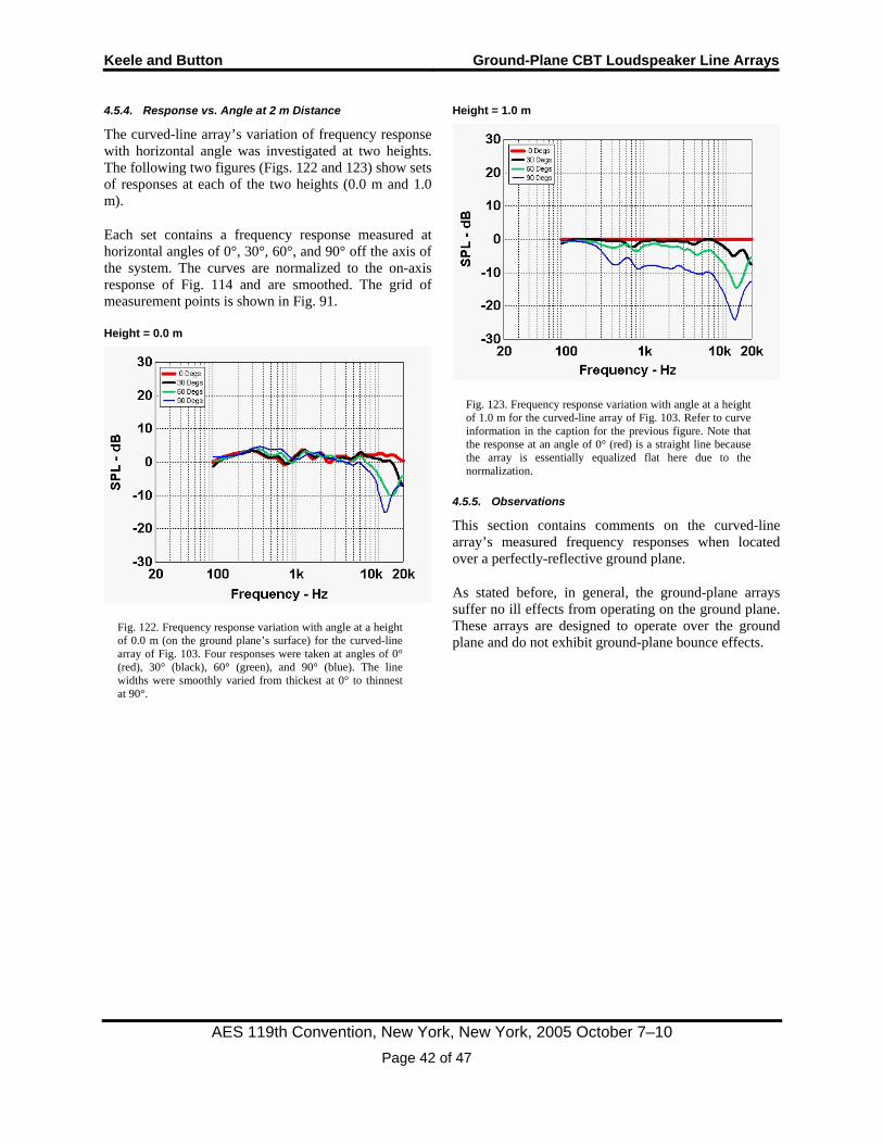
Keele and Button Ground-Plane CBT Loudspeaker Line Arrays
AES 119th Convention, New York, New York, 2005 October 7–10 Page 42 of 47
4.5.4. Response vs. Angle at 2 m Distance
The curved-line array’s variation of frequency response with horizontal angle was investigated at two heights. The following two figures (Figs. 122 and 123) show sets of responses at each of the two heights (0.0 m and 1.0 m).
Each set contains a frequency response measured at horizontal angles of 0°, 30°, 60°, and 90° off the axis of the system. The curves are normalized to the on-axis response of Fig. 114 and are smoothed. The grid of measurement points is shown in Fig. 91.
Height = 0.0 m
Fig. 122. Frequency response variation with angle at a height of 0.0 m (on the ground plane’s surface) for the curved-line array of Fig. 103. Four responses were taken at angles of 0° (red), 30° (black), 60° (green), and 90° (blue). The line widths were smoothly varied from thickest at 0° to thinnest at 90°.
Height = 1.0 m
Fig. 123. Frequency response variation with angle at a height of 1.0 m for the curved-line array of Fig. 103. Refer to curve information in the caption for the previous figure. Note that the response at an angle of 0° (red) is a straight line because the array is essentially equalized flat here due to the normalization.
4.5.5. Observations
This section contains comments on the curved-line array’s measured frequency responses when located over a perfectly-reflective ground plane.
As stated before, in general, the ground-plane arrays suffer no ill effects from operating on the ground plane. These arrays are designed to operate over the ground plane and do not exhibit ground-plane bounce effects.
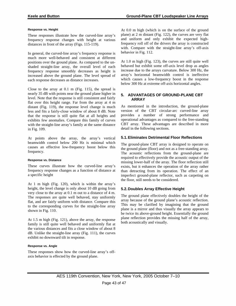
Keele and Button Ground-Plane CBT Loudspeaker Line Arrays
AES 119th Convention, New York, New York, 2005 October 7–10 Page 43 of 47
Response vs. Height
These responses illustrate how the curved-line array’s frequency response changes with height at various distances in front of the array (Figs. 115-119).
In general, the curved-line array’s frequency response is much more well-behaved and consistent at different positions over the ground plane. As compared to the un-shaded straight-line array, the overall level of each frequency response smoothly decreases as height is increased above the ground plane. The level spread of each response decreases as distance increases.
Close to the array at 0.1 m (Fig. 115), the spread is nearly 35 dB with points near the ground plane higher in level. Note that the response is still consistent and fairly flat over this height range. Far from the array at 4 m distant (Fig. 119), the response level change is much less and fits a fairly-close window of about 8 dB. Note that the response is still quite flat at all heights and exhibits few anomalies. Compare this family of curves with the straight-line array’s family at the same distance in Fig. 109.
At points above the array, the array’s vertical beamwidth control below 200 Hz is minimal which causes an effective low-frequency boost below this frequency.
Response vs. Distance
These curves illustrate how the curved-line array’s frequency response changes as a function of distance at a specific height
At 1 m high (Fig. 120), which is within the array’s height, the level change is only about 10 dB going from very close to the array at 0.1 m out to a distance of 4 m. The responses are quite well behaved, stay uniformly flat, and are fairly uniform with distance. Compare this to the corresponding curves for the straight-line array shown in Fig. 110.
At 1.5 m high (Fig. 121), above the array, the response family is still quite well behaved and uniformly flat at the various distances and fits a close window of about 8 dB. Unlike the straight-line array (Fig. 111), the curves exhibit no downward tilt in response.
Response vs. Angle
These responses show how the curved-line array’s off-axis behavior is effected by the ground plane.
At 0.0 m high (which is on the surface of the ground plane) at 2 m distant (Fig. 122), the curves are very flat and uniform and only exhibit the expected high-frequency roll off of the drivers the array is constructed with. Compare with the straight-line array’s off-axis behavior in Fig. 112.
At 1.0 m high (Fig. 123), the curves are still quite well behaved but exhibit some off-axis level drop as angles increase due to the arrays curvature. Below 300 Hz, the array’s horizontal beamwidth control is ineffective which causes a low-frequency boost in the response below 300 Hz at extreme off-axis horizontal angles.
5. ADVANTAGES OF GROUND-PLANE CBT ARRAY
As mentioned in the introduction, the ground-plane version of the CBT circular-arc curved-line array provides a number of strong performance and operational advantages as compared to the free-standing CBT array. These advantages are described in more detail in the following sections.
5.1. Eliminates Detrimental Floor Reflections
The ground-plane CBT array is designed to operate on the ground plane (floor) and not as a free-standing array. The acoustic reflections from the ground-plane are required to effectively provide the acoustic output of the missing lower-half of the array. The floor reflection still exists, but it enhances the operation of the array rather than detracting from its operation. The effect of an imperfect ground-plane reflector, such as carpeting on the floor, still needs to be considered.
5.2. Doubles Array Effective Height The ground plane effectively doubles the height of the array because of the ground plane’s acoustic reflection. This may be clarified by imagining that the ground plane is a mirror and thus visually the array appears to be twice its above-ground height. Essentially the ground plane reflection provides the missing half of the array, both acoustically and visually.
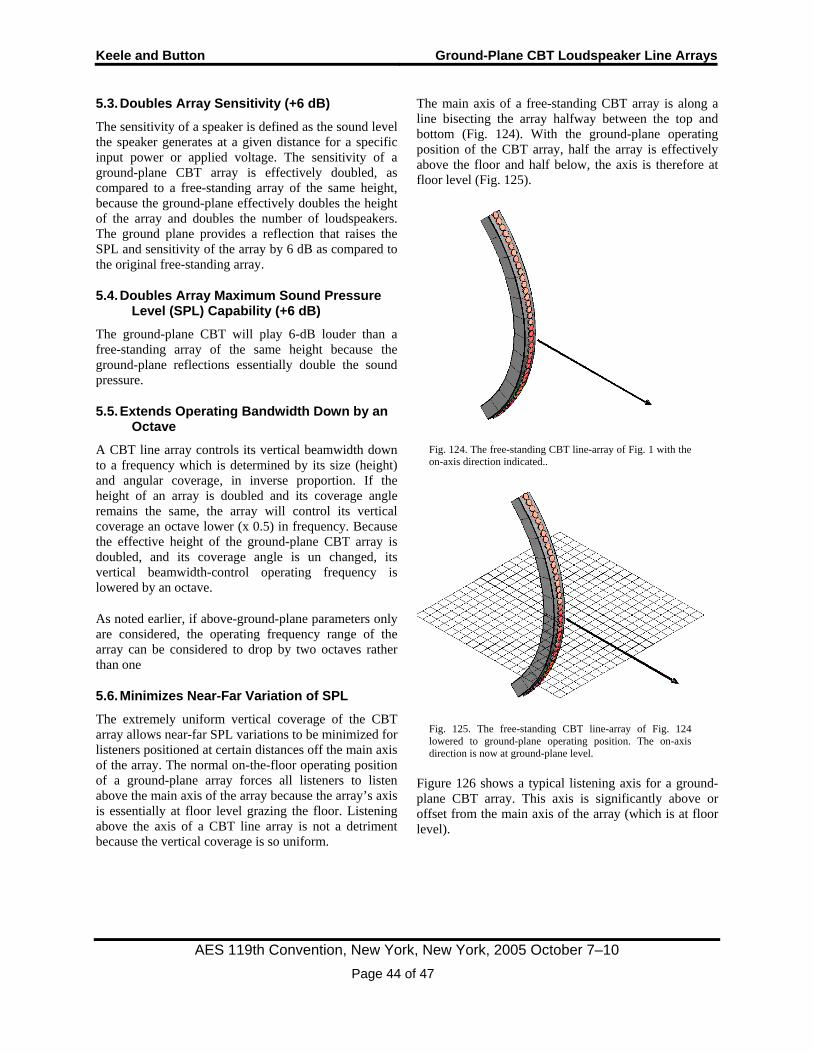
Keele and Button Ground-Plane CBT Loudspeaker Line Arrays
AES 119th Convention, New York, New York, 2005 October 7–10 Page 44 of 47
5.3. Doubles Array Sensitivity (+6 dB)
The sensitivity of a speaker is defined as the sound level the speaker generates at a given distance for a specific input power or applied voltage. The sensitivity of a ground-plane CBT array is effectively doubled, as compared to a free-standing array of the same height, because the ground-plane effectively doubles the height of the array and doubles the number of loudspeakers. The ground plane provides a reflection that raises the SPL and sensitivity of the array by 6 dB as compared to the original free-standing array.
5.4. Doubles Array Maximum Sound Pressure Level (SPL) Capability (+6 dB)
The ground-plane CBT will play 6-dB louder than a free-standing array of the same height because the ground-plane reflections essentially double the sound pressure.
5.5. Extends Operating Bandwidth Down by an Octave
A CBT line array controls its vertical beamwidth down to a frequency which is determined by its size (height) and angular coverage, in inverse proportion. If the height of an array is doubled and its coverage angle remains the same, the array will control its vertical coverage an octave lower (x 0.5) in frequency. Because the effective height of the ground-plane CBT array is doubled, and its coverage angle is un changed, its vertical beamwidth-control operating frequency is lowered by an octave.
As noted earlier, if above-ground-plane parameters only are considered, the operating frequency range of the array can be considered to drop by two octaves rather than one
5.6. Minimizes Near-Far Variation of SPL
The extremely uniform vertical coverage of the CBT array allows near-far SPL variations to be minimized for listeners positioned at certain distances off the main axis of the array. The normal on-the-floor operating position of a ground-plane array forces all listeners to listen above the main axis of the array because the array’s axis is essentially at floor level grazing the floor. Listening above the axis of a CBT line array is not a detriment because the vertical coverage is so uniform.
The main axis of a free-standing CBT array is along a line bisecting the array halfway between the top and bottom (Fig. 124). With the ground-plane operating position of the CBT array, half the array is effectively above the floor and half below, the axis is therefore at floor level (Fig. 125).
Fig. 124. The free-standing CBT line-array of Fig. 1 with the on-axis direction indicated..
Fig. 125. The free-standing CBT line-array of Fig. 124 lowered to ground-plane operating position. The on-axis direction is now at ground-plane level.
Figure 126 shows a typical listening axis for a ground-plane CBT array. This axis is significantly above or offset from the main axis of the array (which is at floor level).
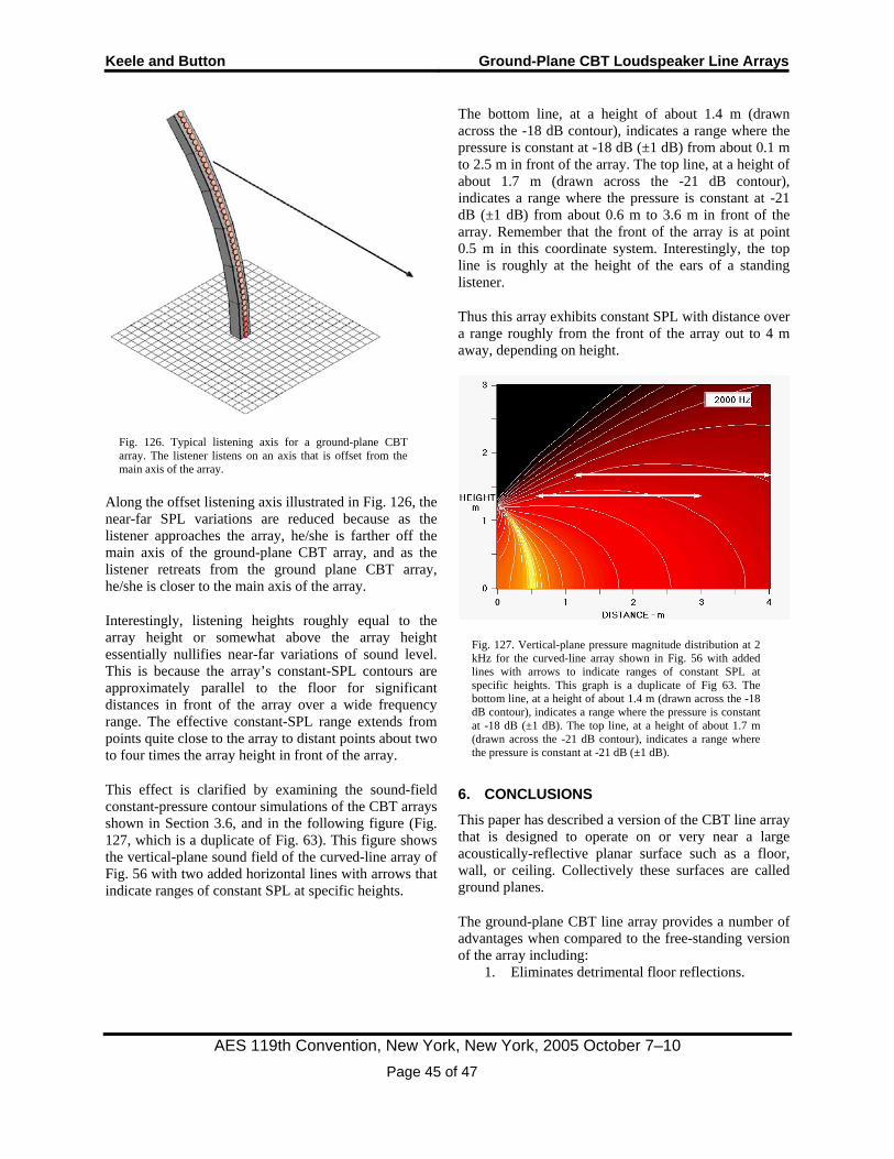
Keele and Button Ground-Plane CBT Loudspeaker Line Arrays
AES 119th Convention, New York, New York, 2005 October 7–10 Page 45 of 47
Fig. 126. Typical listening axis for a ground-plane CBT array. The listener listens on an axis that is offset from the main axis of the array.
Along the offset listening axis illustrated in Fig. 126, the near-far SPL variations are reduced because as the listener approaches the array, he/she is farther off the main axis of the ground-plane CBT array, and as the listener retreats from the ground plane CBT array, he/she is closer to the main axis of the array.
Interestingly, listening heights roughly equal to the array height or somewhat above the array height essentially nullifies near-far variations of sound level. This is because the array’s constant-SPL contours are approximately parallel to the floor for significant distances in front of the array over a wide frequency range. The effective constant-SPL range extends from points quite close to the array to distant points about two to four times the array height in front of the array.
This effect is clarified by examining the sound-field constant-pressure contour simulations of the CBT arrays shown in Section 3.6, and in the following figure (Fig. 127, which is a duplicate of Fig. 63). This figure shows the vertical-plane sound field of the curved-line array of Fig. 56 with two added horizontal lines with arrows that indicate ranges of constant SPL at specific heights.
The bottom line, at a height of about 1.4 m (drawn across the -18 dB contour), indicates a range where the pressure is constant at -18 dB (±1 dB) from about 0.1 m to 2.5 m in front of the array. The top line, at a height of about 1.7 m (drawn across the -21 dB contour), indicates a range where the pressure is constant at -21 dB (±1 dB) from about 0.6 m to 3.6 m in front of the array. Remember that the front of the array is at point 0.5 m in this coordinate system. Interestingly, the top line is roughly at the height of the ears of a standing listener.
Thus this array exhibits constant SPL with distance over a range roughly from the front of the array out to 4 m away, depending on height.
Fig. 127. Vertical-plane pressure magnitude distribution at 2 kHz for the curved-line array shown in Fig. 56 with added lines with arrows to indicate ranges of constant SPL at specific heights. This graph is a duplicate of Fig 63. The bottom line, at a height of about 1.4 m (drawn across the -18 dB contour), indicates a range where the pressure is constant at -18 dB (±1 dB). The top line, at a height of about 1.7 m (drawn across the -21 dB contour), indicates a range where the pressure is constant at -21 dB (±1 dB).
6. CONCLUSIONS This paper has described a version of the CBT line array that is designed to operate on or very near a large acoustically-reflective planar surface such as a floor, wall, or ceiling. Collectively these surfaces are called ground planes.
The ground-plane CBT line array provides a number of advantages when compared to the free-standing version of the array including:
1. Eliminates detrimental floor reflections.
Keele and Button Ground-Plane CBT Loudspeaker Line Arrays
AES 119th Convention, New York, New York, 2005 October 7–10 Page 46 of 47
2. Effectively doubles array height without increasing physical height.
3. Doubles array sensitivity (+6 dB). 4. Doubles array maximum sound pressure level
(SPL) capability (+6 dB). 5. Extends operating bandwidth down by an
octave (or two octaves depending on how the beamwidth is defined).
6. Minimizes near-far variation of SPL.
Conversely, these advantages can be applied in reverse to create an array one-half the size with the same performance as the full-size free-standing array, when a ground plane is available for use.
This paper has reinforced these claims via simulation and measurements.
Vertical-plane sound-field simulations were accomplished on several different types of point-source configurations including:
1. A single point source located above a non-reflective ground plane (free space).
2. A single point source located above a perfectly-reflective ground plane.
3. A vertically-oriented straight-line source with and without Hann shading located resting on a perfectly-reflective ground plane.
4. A circular-arc curved-line source with and without Legendre shading located with its bottom resting on a perfectly-reflective ground plane. The former is a physically-curved CBT array.
5. A delay-curved straight-line source with and without Legendre shading located resting on perfectly-reflective ground plane. The former is a delay-curved CBT array.
These simulations show the excellence of the ground-plane CBT array in creating extremely-uniform frequency-invariant sound fields when operated above a ground plane.
Detailed over-the-ground-plane frequency-response measurements were made of three systems that included:
1. A conventional two-way compact monitor, 2. An experimental 1.25 m tall ground-plane
straight-line array containing 36 full-range miniature drivers with no shading (all drivers operating with equal input levels), and
3. An experimental 1.1 m tall ground-plane circular-arc curved-line CBT array containing 36 full-range miniature drivers with Legendre shading (bottom driver on full with level decreasing with height).
These measurements illustrated the clear superiority of the ground-plane CBT array to provide frequency responses that change very little with height, distance, and lateral off-axis angle.
What this paper did not address was the effect of the complex acoustic impedance of the ground plane and its effect on the sound radiation of the ground-plane arrays. The simulations were done assuming a perfectly-reflective ground plane. Likewise, the measurements were accomplished over an extremely-rigid highly-reflective tiled surface.
Questions such as: What happens when the array is operated over a real floor with added carpet the provides high-frequency absorption?, or What effect has a non-rigid ground-plane surface have on the low-frequency efficiency and pattern control of the array?, have not been answered. These are topics for later research.
[Note: one author (Keele) does have some limited experience with measuring the frequency response of a CBT array over a carpeted surface (with a real-time third-octave spectrum analyzer). The main effect was a rolloff of higher frequencies at points close to the floor and particularly for grazing-incidence sound waves. The frequency response at points about 0.1m or higher above the floor did not seem to be affected at all as compared to a non-carpeted surface.]
7. ACKNOWLEDGEMENTS
This work was supported by Harman/Becker Automotive Systems and JBL Professional (both divisions of Harman International Industries) and is the subject of several pending patents.
8. REFERENCES
[1] P. H. Rogers, and A. L. Van Buren, "New Approach to a Constant Beamwidth Transducer," J. Acous. Soc. Am., vol. 64, no. 1, pp. 38-43 (1978 July).
Keele and Button Ground-Plane CBT Loudspeaker Line Arrays
AES 119th Convention, New York, New York, 2005 October 7–10 Page 47 of 47
[2] J. Jarzynski and W. J. Trott, “Array Shading for Broadband Constant Directivity Transducer,” J. Acous. Soc. Am., vol. 64, no. 5, pp. 1266-1269 (1978 November).
[3] A. L. Van Buren, L. D. Luker, M. D. Jevnager, and A. C. Tims, "Experimental Constant Beamwidth Transducer," J. Acous. Soc. Am., vol. 73, no. 6, pp. 2200-2209 (1983 June).
[4] D. B. Keele, Jr., “The Application of Broadband Constant Beamwidth Transducer (CBT) Theory to Loudspeaker Arrays,” 109th Convention of the Audio Engineering Society, Preprint 5216 (Sept. 2000).
[5] D. B. Keele, Jr., “Implementation of Straight-Line and Flat-Panel Constant Beamwidth Transducer (CBT) Loudspeaker Arrays Using Signal Delays,” 113th Convention of the Audio Engineering Society, Preprint 5653 (Oct. 2002).
[6] D. B. Keele, Jr., “The Full-Sphere Sound Field of Constant Beamwidth Transducer (CBT) Loudspeaker Line Arrays,” J. Aud. Eng. Soc., vol. 51, no. 7/8., pp. 611-624 (2003 July/August).
[7] D. B. Keele, Jr., “Practical Implementation of Constant Beamwidth Transducer (CBT) Loudspeaker Circular-Arc Line Arrays,” presented at the 115th Convention of the Audio Engineering Society, New York, Preprint ???? (Oct. 2003).
[8] J. B. Allen and D. A. Berkley, "Image Method for Efficiently Simulating Small-Room Acoustics." J. Acoust. Soc. of Am., vol. 65, pp. 943-950 (Apr. 1979).
[9] F. J. Harris, "On the Use of Windows for Harmonic Analysis with the Discrete Fourier Transform," Proceedings of the IEEE, Vol. 66, No.1, pp. 51-83, (Jan. 1978).
[10] A. Farina, “Simultaneous Measurement of Impulse Response and Distortion with a Swept-Sine Technique,” presented at the 108P
thP Convention of
the Audio Engineering Society, New York, Preprint 5093 (Apr. 2000).