A Two Step Model for Linear Prediction,

with Connections to PLS

Ying Li

Faculty of Natural Resources and Agricultural Sciences,Department of Energy and Technology,

Uppsala

Licentiate Thesis

Swedish University of Agricultural Sciences

Uppsala 2011

SUAS, Swedish University of Agricultural SciencesDepartment of Energy and Technology

Report (Department of Energy and Technology)

Licentiate thesis/Report 036

ISSN, 1654-9406

ISBN, 978-91-576-9055-5

c© 2011 Ying Li, Uppsala

Print: SLU Service/Repro, Uppsala 2011

2

Till baba, mama.

3

4

A Two Step Model for Linear Prediction,with Connections to PLS

Abstract

In the thesis, we consider prediction of a univariate response variable,especially when the explanatory variables are almost collinear. A twostep approach has been proposed. The first step is to summarize theinformation in the explanatory variables via a bilinear model with aKrylov structured design matrix. The second step is the predictionstep where a conditional predictor is applied. The two step approachgives us a new insight in partial least squares regression (PLS). Explicitmaximum likelihood estimators of the variances and mean for the ex-planatory variables are derived. It is shown that the mean square errorof the predictor in the two step model is always smaller than the onein PLS. Moreover, the two step model has been extended to handlegrouped data. A real data set is analyzed to illustrate the performanceof the two step approach and to compare it with other regularized meth-ods.

Keywords: A Two Step Model, Krylov Space, MLE, PLS.

Author’s address:Ying LiSLU, Department of Energy and Technology,Box 7032, 75007 Uppsala Sweden.E-mail : Ying.li@slu.se

5

6

Sammanfattning

Prediktion ar temat for avhandlingen. Givet att man har observerat bak-grundsvariabler sa vill man med hjalp av dessa forutsaga en respons variabel.Problemet ar att ofta har man ett stort antal variabler som aven samvarierarvilket gor det svart att utnyttja informationen i dessa. Detta ar ett valkantproblem och under ca 50 ar har man forsokt att forbattra prediktionsme-toderna.

I denna avhandling har jag delat in prediktionsproblemet i tva steg. Detforsta steget sammanfattas informationen i bakgrundsvariablerna via en mul-tivariat bilinjar modell. Detta sker genom att ett fatal nya variabler skapaseller att nagra fa vasentliga bakgrundsvariabler selekteras. Pa sa satt reduc-eras den ursprungliga datamangden som kan besta av hundratals variabler tillen mangd bestaende av hogst ett tiotal variabler. I det andra steget, predik-tionssteget, sker prediktionen genom klassisk betingning med avseende pa denreducerade datamangden for att pa sa vis erhalla en predicerad respons.

Avhandlingen baseras pa tre uppsatser. Tva av dem innehaller teoretiskaresultat och i den tredje gjordes en jamforelse mellan att antal prediktions-metoder, inklusive en ny tvastegs-ansats, dar relationen mellan responsvari-ablerna laktat, etanol och 2,3-butandiol och bagrundvariablerna i form avabsorptionsband fran FTIR-analys (FTIR-Fourier transform infrarod spek-troskopi) studerades.

Avhandlingen har inspirerats av PLS (partial least squares) ansatsen. Ettnytt argument har upptackts som motiverar anvandandet av PLS genom attutnyttja Caley-Hamiltons sats som sager att varje kvadratisk matris “upp-fyller sin egen karakteristiska ekvation”. PLS ar egentligen en algoritmiskansats och det ar valkant att PLS genererar en bas i ett Krylov rum. Viden sammanfattning av informationen i bakgrundsvariablerna anvander utnyt-tjas Krylovrummet. Avhandlingen utnyttjar darefter teori fran multivariata(bi)linjara modeller och ett av huvudresultaten ar att maximum likelihood–skattningar kan erhallas vilket ar langt ifran sjalvklart. Prediktionen baseraspa dessa skattningar. Vidare kan de bilinjara modellerna inkludera faktorersom motsvarar faktorer i klassisk variansanalys sasom blockningsfaktorer foratt tex kunna studera gruppeffekter.

I den tillampade delen av arbetet har tvastegs-ansatsen studerats i forhal-lande till variabelselektionsmetoder, lasso-och ridge-regression, PLS och vanliglinjar prediktion. For FTIR-data hade ridge-regressionen den basta predik-tionsformagan medan tvastegs-metoden var bast nar det gallde att samman-fatta informationen i bakgrundsvariablerna.

7

8

Contents

List of papers in the thesis 11

1 Introduction 13

2 The linear model 14

3 The PLS algorithm 14

4 Brief overview of regularization methods 16

4.1 Numerical approaches . . . . . . . . . . . . . . . . . . . . . . . 164.2 Shrinkage property . . . . . . . . . . . . . . . . . . . . . . . . . 18

5 Summary of papers 19

5.1 Paper I . . . . . . . . . . . . . . . . . . . . . . . . . . . . . . . 195.2 Paper II . . . . . . . . . . . . . . . . . . . . . . . . . . . . . . . 205.3 Paper III . . . . . . . . . . . . . . . . . . . . . . . . . . . . . . 22

6 Discussion 22

6.1 Contributions . . . . . . . . . . . . . . . . . . . . . . . . . . . . 226.2 Future work . . . . . . . . . . . . . . . . . . . . . . . . . . . . . 23

Acknowledgement 24

References 25

9

10

List of papers

This thesis is based on the work contained in the following papers, referredto by Roman numerals in the text:

I Ying Li and Dietrich von Rosen (2011), Maximum likelihood estimatorsin a two step model for PLS. Communications in Statistics - Theory andMethods, accepted

II Ying Li and Dietrich von Rosen (2011), A two step model for linear pre-diction with group effect. Report LiTH-MAT-R-2011/16-SE, LinkopingUniversity

III Ying Li, Dietrich von Rosen and Peter Uden (2011), A comparison of pre-diction methods for silage composition from spectral data. Manuscript

11

12

1 INTRODUCTION

1 Introduction

Linear regression is the core statistical method used in a variety of scientificapplications. It concentrates on building relations between a set of explana-tory variables and a response variable. It is used to predict a future responseobservation from a given observation of explanatory variables. In this thesis,we mainly focus on the prediction aspect.

One common choice in prediction is to use the ordinary least squares (OLS)estimator. The Gauss-Markov theory asserts that the least squares estimatoris BLUE (Best Linear Unbiased Estimator). However, unbiasedness is notnecessarily a wise criterion for estimators, especially when it concerns predic-tion. The prediction accuracy is related to the mean square error (MSE) ofthe estimators. The mean square error is the sum of the variance and thesquared bias. The MSE of OLS estimator is the smallest among all linear un-biased estimators. However when the variables are collinear or near-collinear,there exist estimators with small bias but large variance reduction. The over-all prediction accuracy is then better than that of an OLS estimator. Suchestimators usually are referred to as shrinkage estimators or regularized esti-mators.

Many real-life application produce collinear data. For example, in chemo-metrics, the aim is usually to build a predictive relation between the concen-tration of one compound and a set of absorbance values of wavelengths of aspectra. The number of wavelengths is large and the absorbance values arecorrelated. In this case, the classical OLS often needs to be modified to fulfillpractical requirements.

Several regularization methods have been proposed, such as ridge regres-sion (RR), lasso regression (Lasso), principal component regression (PCR)and partial least squares regression (PLS); for a review see Brown (1993) andSundberg (1999). Among others, PLS is considered in some detail in thethesis. Originally the idea of PLS was intuitively introduced by Wold (Wold,1966) as an algorithm. Nowadays, it plays a dominating role in chemometrics.With the contributions of several mathematicians and statisticians (Helland,1988,1990; Stone and Brooks, 1990; Frank and Friedman, 1993; Butler andDenham, 2000), many pros and cons of PLS can be listed. In particular,Butler and Denham (2000) have shown that PLS can not be an optimal re-gression model in any reasonable way. Helland (2001) stated, the only possiblepath left towards some kind of optimality, it seems, is by first trying to find agood motivation for the population model and the possibly finding an optimalestimator under this model, which coincides with the aim of the present thesis.

In the thesis, we have developed a two step model. In the first step, infor-mation in the explanatory variable is extracted with the help of a multivariatelinear model where a Krylov design matrix is used, which is inspired by PLS.In the second step, the prediction step, a conditional approach is applied. Thetwo step model is closely connected to the PLS population approach.

The linear model is set up in Section 2, and in Section 3, the PLS algorithmis introduced. In Section 4, a brief review of regularizationmethods is given, in

13

3 THE PLS ALGORITHM

particular a numerical approach is considered. The papers, which this thesisis based on, are summarized in Section 5. Contributions and future works arediscussed at the end.

2 The linear model

Let (x′, y)′ be a (p+1)−dimensional random vector. It follows a multivariatedistribution with E[x] = µx and E[y] = µy where E[·] denotes the mean,D[x] = Σ, supposed to be positive definite, where D[·] denotes the disper-sion (variance) and C[x, y] = ω, where C[·] denotes the covariance. Undernormality, (

x

y

)∼ N(p+1)

((µx

µy

),

(Σ ω

ω′

σ2y

)). (2.1)

When all the parameters are known, the best linear predictor is conditionalexpectation of y given x, i.e.

y = E(y|x) = ω′Σ−1(x− µx) + µy. (2.2)

Let β′ = ω′Σ−1. Typically a sample (x′, y)′i, i = 1, · · · , n, is used to fit themodel. Thus with the n observations yield a data matrix X: p × n and anobservation vector y: n× 1. Then it is natural to replace the predictor (2.2)by its empirical version

y′

L = s′xyS−1xx (X− X) + y′, (2.3)

where β′

= s′xySxx, and

X = XP1′ , y′ = y′P1′ , P1′ = 1′1/n

sxy = X(I−P1′)y/n, Sxx = X(I−P1′)X′/n.

3 The PLS algorithm

The partial least squares algorithm originated from a system analysis approach(Wold & Joreskog, 1982). As a calibration method in chemometrics , it wasdeveloped by Svante Wold and Harald Martens (Wold et al., 1983). The PLSalgorithm was first presented as a modified NIPALS (Wold, 1966). Since itsimportant role in chemometrics, many approaches have been suggested tomodify the algorithm, in particular from a numerical point of view. Thereare several different versions of the PLS algorithm available: the algorithm byMartens (Næs and Martens, 1985), SIMPLS by de Jong (1993), Kernel PLSby Rannar et al. (1994) and PLSF by Wu & Manne (2000). From a theoreticalpoint of view, these algorithms should lead to the same results. In this thesis,we use the PLS version which was formulated by Helland (1988). This is apopulation version where parameters are known. Then it goes as follows:

14

3 THE PLS ALGORITHM

1. Define starting values for the x residuals ei,

e0 = x− µx.

Do the following steps for i = 1, 2, . . . :

2. Introduce scores ti and weights ωi

ti = e′i−1ωi,

ωi = C[ei−1,y],

3. Determine x loadings pi by least squares

pi =C[ei−1, ti]

D[ti],

4. Find new residualsei = ei−1 − pit

′

i.

At each step a, a linear representation

x = µx + p1t′

1 + p2t′

2 + · · ·+ pat′

a + ea

is obtained. The algorithm implies that

ωa+1 = (I−D[ea−1]ωa(ω′

aD[ea−1]ωa)−ω′

a)ωa, (3.1)

D[ea] = D[ea−1]−D[ea−1]ωa(ω′

aD[ea−1]ωa)−ω′

aD[ea−1]. (3.2)

If Ga is any matrix spanning the column space ζ(ω1 : ω2 : · · · : ωa), we findthe recurrence relations

D[ea] = Σ−ΣGa(G′

aΣGa)−G′

aΣ, (3.3)

ωa+1 = (I−ΣGa(G′

aΣGa)−G′

a)ω1.

Note that ω1 = ω is the covariance between y and x. It is easy to show thatGa defines an orthogonal basis by using (3.1), (3.2) and results for projectionoperators. Alternative proofs of this fact are given in Helland (1988) andHoskuldsson (1988).

Furthermore, by induction we have the identity

ζ(Ga) = ζ(ω1 : ω2 : · · · : ωa) = ζ(ω : Σω : · · · : Σa−1ω).

The space ζ(ω : Σω : · · · : Σa−1ω) is called Krylov space. The PLS predictorat step a equals

ya,PLS = ω′Ga(G′

aΣGa)−G′

a(x− µx) + µy. (3.4)

It is worth noting that when the algorithm stops the Krylov space is Σ-invariant since ωa+1 = 0 or D[ea]ωa = 0 (Kollo & von Rosen, 2005, p.61).

15

4 BRIEF OVERVIEW OF REGULARIZATION METHODS

There are some nice properties of invariant subspace which are helpful forunderstanding PLS and linear models; see, for example, a discussion by vonRosen (1994). As observed by Manne (1987), if the Gram-Schmidt orthogo-nalization algorithm is working on the Krylov space, it will produce the sameorthogonal basis as given by the PLS algorithm.

The sample PLS predictor equals

y′

a,PLS = s′xyGa(Ga

′

SxxGa)−Ga

′

(X− X) + y′, (3.5)

with

Ga = (sxy,Sxxsxy,S2xxsxy, · · · ,Sa−1

xx sxy).

Several available results as the properties of PLS are based on the sampleversion of the PLS predictor.

4 Brief overview of regularization methods

The discussions of regularization methods are mainly going on in two direc-tions. One side is the comparison, in what situation, which method is ex-pected to work better than others. A Monto Carlo study given by Frank andFriedman (1993) compared RR, PCR, PLS with the classical statistical meth-ods OLS and variable subsect selection (VSS). It was concluded that in highcollinearity situations, the performances of RR, PCR and PLS tend to be fairlysimilar and are considerably better than OLS and VSS. The other side is thelinkage among the regularized estimators. Among others, Stone and Brooks(1990) introduced continuum regression, where OLS, PCR and PLS all nat-urally appear as special cases, corresponding to different maximum criteria:correlation, variance, covariance (Sundberg, 1999). Furthermore, the linkagebetween continuum regression and ridge regression was shown by Sundberg(1993). In this section, we will summarize some regularization methods basedon numerical approaches. The aim is to expose a parallel system in order tounderstand the regularization methods from a different angle.

4.1 Numerical approaches

The term regularized emanates form the method of regularization in approxi-mation theory literature (Brown, 1993). Therefore it is worth looking upon allthe methods from using numerical approaches. In my opinion, the motivationsof the methods are quite clear if the aim is to solve a linear system.

The basic solution for a linear system is found by minimizing

‖y −X′β‖22, (4.1)

over a proper subset Rp. If X is collinear and ill-conditioned, the straightfor-ward solution for (4.1) becomes very sensitive. Then one may put constraints

16

4 BRIEF OVERVIEW OF REGULARIZATION METHODS

on the solution, which is a type of regularization. Roughly speaking, regular-ization is a technique for transforming a poorly conditioned problem into astable one (Golub and Van Loan, 1996).

Ridge regression is the solution obtained by minimizing

‖y−X′β‖22 + λ‖β‖22.

Since X is ill-conditioned, the solution ‖β‖22 becomes quite large, which canbe considered as a reason of bad performance. Therefore, ridge regressionincludes λ‖β‖22 as a penalty term, which restricts the scale of the solution.

Another possible way to constrain the parameters is to solve

minV′β=γ

‖y −X′β‖22 ≈ minγ

‖y−X′Vγ‖, (4.2)

where V is a matrix with orthogonal columns. V′β can be considered astransforming the solution β onto a lower dimensional space.

PCA can be obtained by (4.2) using truncated singular value decomposi-tion (truncated SVD). SVD states that any matrix Ap×q can be factorizedas

A = UDV′,

where D = (Dr,0)′, Dr = diag(

√λ1,

√λ2, ...,

√λr),

√λi are the singular

values, r = rank(A), U and V are orthogonal. Truncated SVD use thelargest k singular values in Dk to approximate A as

A ≈ UkDkV′

k,

withU = (Uk,U⊥), whereU⊥ is a p×(p−k) matrix such thatU is orthogonaland similarly V = (Vk,V⊥). So to solve a linear system

minβ

‖Xy −XX′β‖22

needs to be solved, we begin with use truncated SVD so thatXX′ = UkDkU′

k.The Uk is used as a transformation matrix such as U′

kβ = γ. Therefore, thelinear system can be reformulated as

minγ

‖Xy −UkDkU′

kUkγ‖22

= minγ

‖U′Xy −DkIkγ‖22 +r∑

i=k+1

(u′

iXy),

with the solution

γ =

u′1Xy/λ1

u′2Xy/λ2

...u′

kXy/λk

β = Uγ =

k∑

i=1

u′

iXy

λk

ui,

17

4 BRIEF OVERVIEW OF REGULARIZATION METHODS

where β mathematically equals the PCR solution.PLS and Lanczos bidiagonalization (LBD) are mathematically equivalent

(Elden, 2003). The LBD procedure generates a series of matrices Rk =(r1, · · · rk), Qk = (q1, · · · ,qk) and

Zk =

α1 γ1α2 γ2

. . .. . .

αk−1 γk−1

γk

,

which satisfy X′Rk = QkZk. Further, Qk and Rk have orthogonal columnswhich span Krylov structured spaces.

ζ(Qk) = ζ(XX′, (XX′)(Xy), · · · , (XX′)k−1(Xy)),

ζ(Rk) = ζ(X′X, (X′X)(X′Xy), · · · , (X′X)k−1(X′Xy)).

So, if we want to compute the solution for (4.1), LBD provides a naturaltransformation matrix Rk such that R′

kβ = γ. Then the solution γ can beobtained by solving

minγ

‖y −X′Rkγ‖22 = minγ

‖y−QkZkγ‖22 (4.3)

= minγ

‖Q′

ky − Zkγ‖22 + ‖Q′

⊥y‖22, (4.4)

So thatγ = Z−1

k Qky, β = RkZ−1k Qky. (4.5)

It can be shown that above β is mathematically equivalent to the sampleversion PLS predictor.

4.2 Shrinkage property

Based on the estimators derived from numerical approaches, it is convenientto explore the shrinkage property of the regularized estimators. Frank andFriedman (1993) defined the“shrinkage factor”concept to compare the shrink-age behavior of different methods. The general proposed form of estimatorsis

β =

r∑

j=1

f(λj)αjuj ,

where αj = 1λi

u′

jXy,∑r

j=1(1λi

uju′

j) = XX′, r is the rank of X and f(λj)are called shrinkage factors. For MLE, f(λj) = 1. If f(λj) < 1, it will lead to

a reduction on the variance of β, although it may introduce bias as well. It ishoped that an increase in bias is small compared to the decrease in variance,so that the shrinkage is beneficial. Under ridge regression, the shrinkage factor

18

5 SUMMARY OF PAPERS

f(λj) = λj/(λj + λ) is always smaller than 1. For the principal componentregression, f(λj) = 1 if the jth components is included. Otherwise, f(λj) = 0.

The shrinkage property for PLS is peculiar (Butler & Denham, 2000).f(λj) is not always smaller than 1. The smallest eigencomponent can alwaysbe shrunk. f(λ1) > 1, if the number of components in PLS is odd, andf(λj) < 1, if the number of components is even. Bjorkstrom (2010) showedthat the peculiar pattern of alternating shrinkage and inflation is not uniquefor PLS. For a review of shrinkage property of PLS, we refer to Kramer (2007).

5 Summary of papers

5.1 Paper I

In the article, the population PLS predictor is linked to a linear model includ-ing a Krylov design matrix and a two step estimation procedure. The modelin Paper I is

(x

y

)∼ N(p+1)

((µx

µy

),

(Σ ω

ω′

σ2y

)), (5.1)

where the parameters are defined in the same way as in model (2.1).A two step procedure is proposed to predict y from x, especially when

the columns of x are collinear. The motivation of the two step approach isexplained below. The problem of collinearity usually occurs when there is alarge number of explanatory variables. Some of them jointly mirror the samelatent effect and then also influence the response variable, i.e. the explanatoryvariables x are governed by a latent effect and some random effect. So in thefirst step, the information of the x variable is summarized by a linear modelsuch as

x = Aβ + ε, (5.2)

where A is the design matrix, β is the unknown vector and ε ∼ Np(0,Σ).The second step is the prediction step, where y is determined by a conditional

estimator y = ωΣ−1

(x− µx) + µy.If we use A = ΣGa, where Ga is as defined in Section 3, as the design

matrix and use x−µx instead of x in (5.2), then the two step model gives anidentical predictor as the population PLS in (3.4). This observation providesus a natural choice of design matrix for x.

Under a semi-population version of the PLS algorithm, it is assumed thatω and µy are known but Σ and µx are unknown. Moreover, suppose that wehave n pairs (yi,xi) of independent observations. As before we are interestedin the prediction of y given data x0 and this is carried out as

y = ω′Σ−1

(x0 − µx0) + µy, µx0

= Aβ,

where the estimators are obtained from the model

X = Aβ1′

n +E, (5.3)

19

5 SUMMARY OF PAPERS

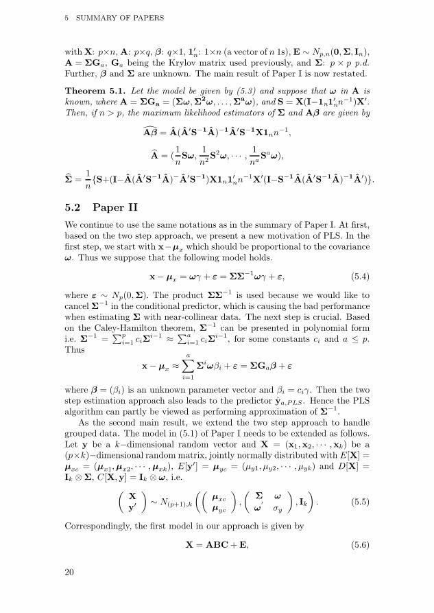
withX: p×n,A: p×q, β: q×1, 1′n: 1×n (a vector of n 1s), E ∼ Np,n(0,Σ, In),

A = ΣGa, Ga being the Krylov matrix used previously, and Σ: p × p p.d.Further, β and Σ are unknown. The main result of Paper I is now restated.

Theorem 5.1. Let the model be given by (5.3) and suppose that ω in A isknown, where A = ΣGa = (Σω,Σ2ω, . . . ,Σaω), and S = X(I−1n1

′nn−1)X′.

Then, if n > p, the maximum likelihood estimators of Σ and Aβ are given by

Aβ = A(A′S−1A)−1A′S−1X1nn−1,

A = (1

nSω,

1

n2S2ω, · · · , 1

naSaω),

Σ =1

n{S+(I−A(A′S−1A)−A′S−1)X1n1

′

nn−1X′(I−S−1A(A′S−1A)−1A′)}.

5.2 Paper II

We continue to use the same notations as in the summary of Paper I. At first,based on the two step approach, we present a new motivation of PLS. In thefirst step, we start with x−µx which should be proportional to the covarianceω. Thus we suppose that the following model holds.

x− µx = ωγ + ε = ΣΣ−1ωγ + ε, (5.4)

where ε ∼ Np(0,Σ). The product ΣΣ−1 is used because we would like tocancel Σ−1 in the conditional predictor, which is causing the bad performancewhen estimating Σ with near-collinear data. The next step is crucial. Basedon the Caley-Hamilton theorem, Σ−1 can be presented in polynomial formi.e. Σ−1 =

∑p

i=1 ciΣi−1 ≈

∑a

i=1 ciΣi−1, for some constants ci and a ≤ p.

Thus

x− µx ≈a∑

i=1

Σiωβi + ε = ΣGaβ + ε

where β = (βi) is an unknown parameter vector and βi = ciγ. Then the twostep estimation approach also leads to the predictor ya,PLS . Hence the PLSalgorithm can partly be viewed as performing approximation of Σ−1.

As the second main result, we extend the two step approach to handlegrouped data. The model in (5.1) of Paper I needs to be extended as follows.Let y be a k−dimensional random vector and X = (x1,x2, · · · ,xk) be a(p×k)−dimensional random matrix, jointly normally distributed with E[X] =µxc = (µx1,µx2, · · · ,µxk), E[y′] = µyc = (µy1, µy2, · · · , µyk) and D[X] =Ik ⊗Σ, C[X,y] = Ik ⊗ ω, i.e.

(X

y′

)∼ N(p+1),k

((µxc

µyc

),

(Σ ω

ω′

σy

), Ik

). (5.5)

Correspondingly, the first model in our approach is given by

X = ABC+E, (5.6)

20

5 SUMMARY OF PAPERS

where X: p × n, A = ΣGa: p × q, B: q × k, C: k × n, k is the number ofgroups, E ∼ Np,n(0,Σ, In), and Σ: p× p is p.d.. The matrices B and Σ areunknown and should be estimated. Then our key result is formulated in thenext theorem.

Theorem 5.2. Let the model be given by (5.6) and suppose that ω in A isknown, where A = ΣGa = (Σω,Σ2ω, . . . ,Σaω) and S = X(I − Pc′)X

′,where Pc′ = C′(CC′)−C. Then, if n > p, the maximum likelihood estimatorsof Σ and AB are given by

AB = A(A′S−1A)−A′S−1XC′(CC′)−,

A = (1

nSω,

1

n2S2ω, · · · , 1

naSaω),

Σ =1

n{S+ (I− A(A′S−1A)−A′S−1)XPc′X

′

×(I− S−1A(A′S−1A)−A′)}.

Proposition 5.1. Assume ω and µy to be known and the given observationsX follow the model in (5.6). The prediction of y is

y′ = ω′Σ−1

(X− µxC) + µ′

y, µx = AB. (5.7)

The third main content in Paper II is the comparison among several meth-ods including our two step approach. We suppose to have n observations froma single group all following the same distribution. The sample version of theleast squares predictor yL, the PLS predictor ya,PLS and the two step pre-dictor ya,TS are

y′

L = s′xyS−1xx (X− X) + y′, (5.8)

y′

a,PLS = s′xyGa(Ga

′

SxxGa)−Ga

′

(X− X) + y′, (5.9)

y′

a,TS = s′xyΣ−1

(X− ABC) + y′. (5.10)

One relation among the predictors for least squares, the PLS algorithm pre-sented in Section 3 and the two step approach is formulated in next theorem.

Theorem 5.3. Let yL, ya,PLS and ya,TS be given by (5.8), (5.9) and (5.10),respectively, and the mean square error (MSE) of any predictor in a calibrationset is defined as E(y − y)′(). Then,

E(y − ya,PLS)′() ≥ E(y − ya,TS)

′() ≥ E(y − yL)′(). (5.11)

The MSE of the two step approach is always smaller than that of PLS.For the comparison of the new observation prediction, a simulation study isincluded. The simulation results indicate that the two step model is better,due to its smaller prediction error and the performance of PLS and TS is notinfluenced much if we have a collinear structure in X.

21

6 DISCUSSION

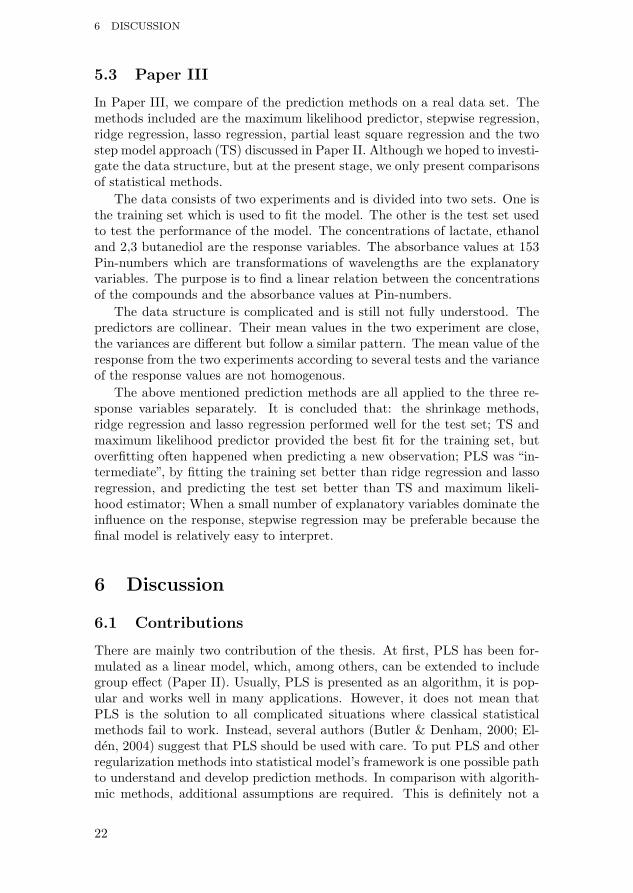
5.3 Paper III

In Paper III, we compare of the prediction methods on a real data set. Themethods included are the maximum likelihood predictor, stepwise regression,ridge regression, lasso regression, partial least square regression and the twostep model approach (TS) discussed in Paper II. Although we hoped to investi-gate the data structure, but at the present stage, we only present comparisonsof statistical methods.

The data consists of two experiments and is divided into two sets. One isthe training set which is used to fit the model. The other is the test set usedto test the performance of the model. The concentrations of lactate, ethanoland 2,3 butanediol are the response variables. The absorbance values at 153Pin-numbers which are transformations of wavelengths are the explanatoryvariables. The purpose is to find a linear relation between the concentrationsof the compounds and the absorbance values at Pin-numbers.

The data structure is complicated and is still not fully understood. Thepredictors are collinear. Their mean values in the two experiment are close,the variances are different but follow a similar pattern. The mean value of theresponse from the two experiments according to several tests and the varianceof the response values are not homogenous.

The above mentioned prediction methods are all applied to the three re-sponse variables separately. It is concluded that: the shrinkage methods,ridge regression and lasso regression performed well for the test set; TS andmaximum likelihood predictor provided the best fit for the training set, butoverfitting often happened when predicting a new observation; PLS was “in-termediate”, by fitting the training set better than ridge regression and lassoregression, and predicting the test set better than TS and maximum likeli-hood estimator; When a small number of explanatory variables dominate theinfluence on the response, stepwise regression may be preferable because thefinal model is relatively easy to interpret.

6 Discussion

6.1 Contributions

There are mainly two contribution of the thesis. At first, PLS has been for-mulated as a linear model, which, among others, can be extended to includegroup effect (Paper II). Usually, PLS is presented as an algorithm, it is pop-ular and works well in many applications. However, it does not mean thatPLS is the solution to all complicated situations where classical statisticalmethods fail to work. Instead, several authors (Butler & Denham, 2000; El-den, 2004) suggest that PLS should be used with care. To put PLS and otherregularization methods into statistical model’s framework is one possible pathto understand and develop prediction methods. In comparison with algorith-mic methods, additional assumptions are required. This is definitely not a

22

6 DISCUSSION

drawback for the approach for applying classical statistical models. Insteadit gives a possibility to perform classical model validation.

The other main contribution is the derivation of explicit maximum likeli-hood estimators. It is a nice mathematical result. In our first step, a Krylovstructured matrix is used as the design matrix, which itself is a function ofthe unknown variance parameter Σ. It is not obvious that there is an explicitsolution. Two important inequalities are used to find an upper bound of thelikelihood function which then also yield the estimators.

6.2 Future work

As mentioned earlier, after putting PLS into the field of linear models, thereare many things to explore. An important one is to define new stoppingrules. Nowadays cross-validation is a common way to decide how many fac-tors should be included. However, it is difficult to study the properties ofparameters selected by cross-validation. In our two step model approach,a Krylov structured matrix is used as the design matrix in the model forexplanatory variables. If PLS stops, the Krylov space turns out to be aninvariant space, with the dimension less than or equal to the original space.Can we define a condition for having an appropriate model which is based onthe Krylov space? Can we use some test, for example, a likelihood ratio test,to compare models with different dimensions? These questions are interestingboth from academic and practical point of view.

The two step model approach is not yet been fully complete. One crucialassumption in the estimation procedure finding MLE is that the covariancebetween x and y is known. Although, using moment estimators one canalways make the method applicable, it is of interest to find a likelihood basedestimator.

In the analysis of spectral data, an interesting phenomenon was noticed.The concentrations of the compound, the response, in the two experimentswere different in their mean and variance. When comparing the absorbancevalues of the Pin-numbers, the explanatory variables, the means of the val-ues at Pin-numbers of the two experiments, were almost the same in severalregions. In the same regions, the variances between the experiments differedbut they followed the same pattern. So it is natural to ask which of the meansor the variances of the predictors play the most essential role in predictingthe response.

23

Acknowledgement

I am heartily thankful to my supervisor Dietrich von Rosen, whose encour-agement, guidance and support from the initial to the final level enabled meto develop an understanding of the subject. Thank you for teaching me nevergive up thinking, which I am still trying. To my second supervisor PeterUden, I appreciate your consistent encourage in my study and your patiencefor the slow process of the data analysis. I can always feel your passion inStatistics.

I want to thank all my colleagues at Department of Energy and Technol-ogy and Department of Animal nutrition and Management. Especially ourbiometry group, Tomas, Idah, Sofia, Fargam, it is always a happy time at thelunch breaks. And to Sofia, I am very happy to work in a room with you andthank you for your help and caring all the time. And Sahar, I enjoy all theconversations with you. To Martin, I appreciate your encouragement when Iwas upset.

I am also grateful to Rauf for answering all my questions, helping me checkEnglish and improving the language in the thesis.

Thank all my Chinese friends studying in Sweden, especially Xia Shen forall the valuable discussion, and Chengcheng, Yuli, it is nice to have companiesin the PhD journey.

The study has been supported by a SLU travel grant.Last but not least to my honey, xiaoxin, I always feel in happiness since

you are here.

24

References

[1] A. Bjorkstrom. Krylov sequences as a tool for analysing iterated regres-sion algorithms. Scand. J. Statist., 37(1):166–175, 2010.

[2] P. J. Brown. Measurement, regression, and calibration. The ClarendonPress Oxford University Press, New York, 1993.

[3] N. A. Butler and M. C. Denham. The peculiar shrinkage properties ofpartial least squares regression. J. Roy. Statist. Soc. Ser. B, 62(3):585–593, 2000.

[4] S. de Jong. Simpls: An alternative approach to partial least squaresregression. Chemometr. Intell. Lab., 18(3):251 – 263, 1993.

[5] L. Elden. Partial least-squares vs. lanczos bidiagonalization-1: analysisof a projection method for multiple regression. Comm. Statist. DataAnalys., 46(1):11 – 31, 2004.

[6] I. E. Frank and J. H. Friedman. A statistical view of some chemometricsregression tools. Technometrics, 35(2):109–135, 1993.

[7] G. H. Golub and C. F. Van Loan. Matrix computations (3rd ed.). JohnsHopkins University Press, Baltimore, MD, USA, 1996.

[8] I. S. Helland. On the structure of partial least squares regression. Comm.Statist. Simulation Comput., 17(2):581–607, 1988.

[9] I. S. Helland. Partial least squares regression and statistical models.Scand. J. Statist., 17(2):97–114, 1990.

[10] I. S. Helland. Some theoretical aspects of partial least squares regression.Chemometr. Intell. Lab., 58(2):97 – 107, 2001.

[11] A. Hoskuldsson. PLS regression methods. J. Chemometr., 2(3):211–228,1988.

[12] T. Kollo and D. von Rosen. Advanced multivariate statistics with matri-ces. Springer, Dordrecht, 2005.

[13] N. Kramer. An overview on the shrinkage properties of partial leastsquares regression. Computational Statistics, 22(2):249–273, 2007.

[14] Y. Li and D. von Rosen. Maximum likelihood estimators in a two stepmodel for PLS. Comm. Statist. A—Theory Methods, Accepted.

[15] R. Manne. Analysis of two partial-least-squares algorithms for multivari-ate calibration. Chemometr. Intell. Lab., 2(1-3):187 – 197, 1987.

[16] T. Naes and H. Martens. Comparison of prediction methods for multi-collinear data. Comm. Statist. Simulation Comput., 14(3):545–576, 1985.

25

[17] S. Rannar, F. Lindgren, P. Geladi, and S. Wold. A PLS kernel algorithmfor data sets with many variables and fewer objects. part 1: Theory andalgorithm. J. Chemometri., 8(2):111–125, 1994.

[18] M. Stone and R. J. Brooks. Continuum regression: cross-validated se-quentially constructed prediction embracing ordinary least squares, par-tial least squares and principal components regression. J. Roy. Statist.Soc. Ser. B, 52(2):237–269, 1990. With discussion and a reply by theauthors.

[19] R. Sundberg. Continuum regression and ridge regression. J. Roy. Statist.Soc. Ser. B, 55(3):653–659, 1993.

[20] R. Sundberg. Multivariate calibration—direct and indirect regressionmethodology. Scand. J. Statist., 26(2):161–207, 1999.

[21] D. von Rosen. PLS, linear models and invariant spaces. Scand. J. Statist.,21(2):179–186, 1994.

[22] H. Wold. Nonlinear estimation by iterative least square procedures. In InResearch Papers Z. in Statistics. Festschrift for J. Ney man F. N. David,ed. Wiley, New York, 1966.

[23] H. Wold and K. G. Joreskog. Systems under indirect observation : causal-ity, structure, prediction. In K.G. Joreskog and H. Wold, editors. North-Holland ; Sole distributors for the U.S.A. and Canada, Elsevier SciencePublishers, Amsterdam; New York, 1982.

[24] S. Wold, H. Martens, and H. Wold. The multivariate calibration problemin chemistry solved by the PLS method. In B. Kagstrom and A. Ruhe,editors, Matrix Pencils, volume 973 of Lecture Notes in Mathematics.Springer Berlin, 1983.

[25] W. Wu and R. Manne. Fast regression methods in a lanczos (or PLS-1)basis. Theory and applications. Chemometr. Intell. Lab., 51(2):145–161,2000.

26