Attachment 1

Great Lakes Coastal Monitoring Project

Draft Standard Operating Procedures and

Field Data Forms

Methods based on

Great Lakes Coastal Wetlands Consortium

Version 5

February, 2016    

Table of Contents: Water Quality SOP 1 Water Quality Field “Cheatsheets” 34 Fish SOP 44 Fish and Macroinvertebrate Field Data Sheets 61 Macroinvertebrate SOP 70 Macroinvertebrate Identification Notes 88 Wetland Vegetation SOP 97 Wetland Vegetation Field Data Sheets 124 Bird SOP and Field Data Sheet 132 Amphibian SOP and Field Data Sheet 137

i  

GLIC: Coastal Monitoring Water Quality SOPs

The following sections describe protocols to be used for field water quality measurements, water sampling, and water sample processing. Standard Operating Procedures (SOPs) will follow the Protocols developed by NRRI-UMD for the National Park Service’s Great Lakes Network (Elias et al. 2008; see below). Relevant sections applicable to shallow water systems were extracted from this document and are reproduced below. Sample collection locations: Chemical/physical measurements will be made in each vegetation type where fish and macroinvertebrate data are collected. Fish and macroinvertebrates are collected by vegetation zone; water quality should be collected in association with fyke nets, one water quality sample per vegetation zone. In the event that fyke nets are not set due to very shallow depth, but invertebrates are collected, then a water quality sample should also be collected from that zone. These samples are required. Crews have the option of taking water quality meter samples at each individual fyke net location (or invertebrate dip net replicate point if fyke nets are not set in that zone). This additional sampling effort is recommended if vegetation patches forming the zone are separated rather than contiguous. Water quality data collection is critical at each wetland, but parameters will be classified as critical, recommended, or supplementary on an individual parameter-by-parameter basis in this section. Defining parameters as "critical" does not mean that biological samples should not be taken at a site if water quality parameters cannot be taken because, for example, the DO sensor on the meter is malfunctioning. Every attempt should be made to get critical measurements, including borrowing equipment from a nearby field crew and obtaining a replacement meter as soon as possible. We also define water quality parameters in terms of 1) field measurements using instruments with sensors used at the site, 2) parameters requiring analysis of a water sample either the evening or the day after the sample was collected, or 3) parameters measured at one of our project water quality laboratories. Critical:

Field: temperature, dissolved oxygen, pH, specific conductivity Lab: alkalinity, turbidity, soluble reactive phosphorus (SRP), [nitrate+nitrite]-nitrogen,

ammonium-nitrogen, chlorophyll-a Recommended:

Field: transparency tube clarity Lab: total nitrogen (TN), total phosphorus (TP), chloride, color

Supplementary:

Field: oxidation-reduction potential (redox), in situ chlorophyll fluorescence Lab: Sediment percent organic matter

In general, two or three vegetation zones will be sampled by fish and macroinvertebrate crews in each wetland, although four zones are possible. The basic water quality sampling design is based primarily on the placement of three fyke nets within each vegetation zone at a site. If fyke nets

1

ii  

cannot be set in a zone, then macroinvertebrate sampling points will be used instead as water quality sampling locations. Water quality data will be collected from fyke net or macroinvertebrate locations as follows:

Field: critical, recommended, and supplementary measurements will be made at the first net set location within each vegetation zone. It is recommended that water quality measurements be made at each net set within the zone, but only one location is required.

Lab: water will be collected from each of the fyke net locations within a vegetation zone

and combined to form a single composite sample, which will be analyzed for critical and recommended water quality parameters.

2

iii  

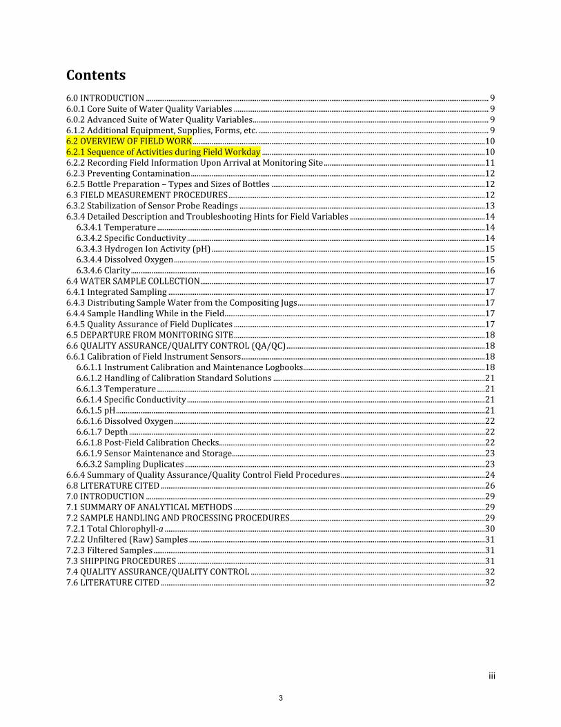
Contents6.0INTRODUCTION.......................................................................................................................................................................................96.0.1CoreSuiteofWaterQualityVariables........................................................................................................................................96.0.2AdvancedSuiteofWaterQualityVariables..............................................................................................................................96.1.2AdditionalEquipment,Supplies,Forms,etc............................................................................................................................96.2OVERVIEWOFFIELDWORK............................................................................................................................................................106.2.1SequenceofActivitiesduringFieldWorkday.......................................................................................................................106.2.2RecordingFieldInformationUponArrivalatMonitoringSite......................................................................................116.2.3PreventingContamination.............................................................................................................................................................126.2.5BottlePreparation–TypesandSizesofBottles..................................................................................................................126.3FIELDMEASUREMENTPROCEDURES.........................................................................................................................................126.3.2StabilizationofSensorProbeReadings...................................................................................................................................136.3.4DetailedDescriptionandTroubleshootingHintsforFieldVariables........................................................................146.3.4.1Temperature...............................................................................................................................................................................146.3.4.2SpecificConductivity...............................................................................................................................................................146.3.4.3HydrogenIonActivity(pH)..................................................................................................................................................156.3.4.4DissolvedOxygen......................................................................................................................................................................156.3.4.6Clarity.............................................................................................................................................................................................16

6.4WATERSAMPLECOLLECTION........................................................................................................................................................176.4.1IntegratedSampling.........................................................................................................................................................................176.4.3DistributingSampleWaterfromtheCompositingJugs....................................................................................................176.4.4SampleHandlingWhileintheField...........................................................................................................................................176.4.5QualityAssuranceofFieldDuplicates......................................................................................................................................176.5DEPARTUREFROMMONITORINGSITE......................................................................................................................................186.6QUALITYASSURANCE/QUALITYCONTROL(QA/QC)..........................................................................................................186.6.1CalibrationofFieldInstrumentSensors..................................................................................................................................186.6.1.1InstrumentCalibrationandMaintenanceLogbooks.................................................................................................186.6.1.2HandlingofCalibrationStandardSolutions.................................................................................................................216.6.1.3Temperature...............................................................................................................................................................................216.6.1.4SpecificConductivity...............................................................................................................................................................216.6.1.5pH.....................................................................................................................................................................................................216.6.1.6DissolvedOxygen......................................................................................................................................................................226.6.1.7Depth..............................................................................................................................................................................................226.6.1.8Post‐FieldCalibrationChecks..............................................................................................................................................226.6.1.9SensorMaintenanceandStorage.......................................................................................................................................236.6.3.2SamplingDuplicates................................................................................................................................................................23

6.6.4SummaryofQualityAssurance/QualityControlFieldProcedures.............................................................................246.8LITERATURECITED.............................................................................................................................................................................267.0INTRODUCTION.....................................................................................................................................................................................297.1SUMMARYOFANALYTICALMETHODS......................................................................................................................................297.2SAMPLEHANDLINGANDPROCESSINGPROCEDURES........................................................................................................297.2.1TotalChlorophyll‐a...........................................................................................................................................................................307.2.2Unfiltered(Raw)Samples..............................................................................................................................................................317.2.3FilteredSamples.................................................................................................................................................................................317.3SHIPPINGPROCEDURES....................................................................................................................................................................317.4QUALITYASSURANCE/QUALITYCONTROL.............................................................................................................................327.6LITERATURECITED.............................................................................................................................................................................32

3

iv  

National Park Service U.S. Department of the Interior Natural Resource Program Center

Water Quality Monitoring Protocol for Inland Lakes

Great Lakes Inventory and Monitoring Network

Version 1.0

Natural Resource Technical Report NPS/GLKN/NRTR-2008/109 Joan Elias National Park Service Great Lakes Inventory and Monitoring Network 2800 Lake Shore Drive East Ashland, Wisconsin 54806 joan_elias@nps.gov

and

Richard Axler and Elaine Ruzycki Center for Water and the Environment Natural Resources Research Institute University of Minnesota Duluth 5013 Miller Trunk Highway Duluth, Minnesota 55811-1442 June 2008 U.S. Department of the Interior

4

v  

National Park Service Natural Resource Program Center Fort Collins, Colorado

The Natural Resource Publication series addresses natural resource topics that are of interest and applicability to a broad readership in the National Park Service and to others in the management of natural resources, including the scientific community, the public, and the NPS conservation and environmental constituencies. Manuscripts are peer-reviewed to ensure that the information is scientifically credible, technically accurate, appropriately written for the intended audience, and is designed and published in a professional manner.

The Natural Resources Technical Reports series is used to disseminate the peer-reviewed results of scientific studies in the physical, biological, and social sciences for both the advancement of science and the achievement of the National Park Service’s mission. The reports provide contributors with a forum for displaying comprehensive data that are often deleted from journals because of page limitations. Current examples of such reports include the results of research that addresses natural resource management issues; natural resource inventory and monitoring activities; resource assessment reports; scientific literature reviews; and peer reviewed proceedings of technical workshops, conferences, or symposia.

Views, statements, findings, conclusions, recommendations and data in this report are solely those of the author(s) and do not necessarily reflect views and policies of the U.S. Department of the Interior, NPS. Mention of trade names or commercial products does not constitute endorsement or recommendation for use by the National Park Service.

Printed copies of reports in these series may be produced in a limited quantity and they are only available as long as the supply lasts. This report is also available from the Natural Resource Publications Management website (http://www.nature.nps.gov/publications/NRPM) on the Internet or by sending a request to the address on the back cover.

Please cite this publication as: Elias, J. E, R. Axler, and E. Ruzycki. 2008. Water quality monitoring protocol for inland lakes. Version 1.0. National Park Service, Great Lakes Inventory and Monitoring Network. Natural Resources Technical Report NPS/GLKN/NRTR—2008/109. National Park Service, Fort Collins, Colorado. NPS D-77, June 2008

5

vi  

Note: The Inland Lakes Water Quality Monitoring Protocol consists of the following: 1. Protocol Narrative 2. Standard Operating Procedures SOP #1: Pre-season Preparation SOP #2: Training and Safety SOP #3: Using the GPS SOP #4: Measuring Water Level SOP #5: Decontamination of Equipment to Remove Exotic Species SOP #6: Field Measurements and Water Sample Collection SOP #7: Processing Water Samples and Analytical Laboratory Requirements SOP #8: Data Entry and Management SOP #9: Data Analysis SOP #10: Reporting SOP #11: Post- Season Procedures SOP #12: Quality Assurance/Quality Control SOP #13: Procedure for Revising the Protocol

6

vii  

Standard Operating Procedure #6: Field Measurements and Water Sample Collection Version 1.1 In Water Quality Monitoring Protocol for Inland Lakes Prepared by Richard Axler and Elaine Ruzycki Center for Water and the Environment Natural Resources Research Institute University of Minnesota-Duluth 5013 Miller Trunk Highway Duluth, Minnesota 55811 and Joan Elias (contact author) National Park Service Great Lakes Inventory and Monitoring Network 2800 Lake Shore Drive East Ashland, Wisconsin 54559 joan_elias@nps.gov March 2010 Suggested citation: Axler, R., E. Ruzycki, and J.E. Elias. 2010. Standard operating procedure #6, Field measurements and water sample collection, Version 1.1. in Elias, J.E., R. Axler, and E. Ruzycki. 2008. Water quality monitoring protocol for inland lakes, Version 1.0. National Park Service, Great Lakes Network, Ashland, Wisconsin. NPS/MWR/GLKN/NRTR—2008/109. National Park Service, Fort Collins, Colorado.

7

viii  

Acknowledgements

Combinations of existing protocols were used to develop this standard operating procedure for measuring the required water quality field parameters for the Great Lakes Network (GLKN). We consulted protocols written for the EPA (Baker et al. 1997), USGS (Hoffman et al. 2005, USGS 2005), and this and other NPS networks (Magdalene et al. 2007; O’Ney 2005); an on-line curriculum for monitoring water quality (WOW 2004); and NPS internal documents (Irwin 2006, 2004; Penoyer 2003; and the WRD website [http://www.nature.nps.gov/water/VitalSignsGuidance.cfm]). We wish to acknowledge these sources and thank them for the valuable contribution that they have made to this document.

8

9  

6.0 Introduction

Field measurements should represent, as closely as possible, the natural condition of the surface water at the time of sampling. Experience with and knowledge of the sampling equipment and the collection, storage, and processing of water samples for subsequent laboratory analyses are critical for collecting data of high quality. To ensure consistent, high-quality data, always:

・Make field measurements only with calibrated instruments that have been error-checked.

・Maintain a permanent log book for each field instrument for recording calibrations and repairs.

Review the log book before leaving for the field. This book should also be used for recording results of pre-and post-calibration checks as well as housing copies of results from alternate measurement sensitivity (AMS) checks, if applicable.

・Test each instrument (meters and sensors) before leaving for the field. Become familiar with

new instruments and new measurement techniques before collecting data.

・Have backup instruments readily available and in good working condition, whenever possible.

・Follow quality assurance/quality control procedures. Such protocols are mandatory for every

data collection effort, and include practicing good field procedures and implementing quality-control checks. Make field measurements in a manner to minimize artifacts that can bias the result.

6.0.1 Core Suite of Water Quality Variables The core field variables are temperature, specific conductance, pH, water level, and dissolved oxygen. To this mandated suite, add a measure of water clarity. Water clarity will be measured with a transparency tube.

6.0.2 Advanced Suite of Water Quality Variables The advanced suite variables consist of total phosphorus, total nitrogen, nitrate+nitrite-nitrogen, ammonia-nitrogen, chloride, alkalinity, and total chlorophyll-a. The methods for collecting water samples for these variables are described in Section 6.5.

6.1.2 Additional Equipment, Supplies, Forms, etc. Refer to the checklist of supplies and equipment needed for field sampling (Table 2) prior to each sampling trip. Keep on hand all necessary forms, calibration logbooks, field logbooks, field data sheets, procedural manuals, and equipment instructional manuals.

9

10  

Table 2. Field supplies and equipment checklist  

  Equipment and Supplies 

  Field notebook, pencils and pen (waterproof ink)  

  New field forms on waterproof paper  

 Up‐to‐date field folders containing recent data sheets for field comparison (copies only; never take originals in the field) 

  Multiparameter instrument (calibrated), calibration standards, data logger  

  Calibration logbook for each instrument  

  All maintenance parts and calibration standards for field instruments  

 Backup instruments in case of electronic failure of multiprobe (for example: YSI 85 [T‐DOSC25] or equivalent, YSI 200 [T‐DO], Hannah Dist3 [SC25], armored NIST certified thermometer [°C], portable pH meter) 

  Transparency tube 

  Secchi disk and metered line (marked at 0.5 m intervals) 

  Composting jug and other bottles 

 Sonde with barometric pressure sensor, weather radio barometer, or other way to obtain barometric pressure 

  Pocket calculator  

  Extra batteries for all field equipment (multiparameter probe, calculator, GPS, etc.)  

  Rain gear  

  First aid kit 

  Personal flotation device(s) 

  Field trip itinerary  

  Cellular phone 

  Digital camera with extra flash cards and battery  

  Map(s) of station location, preferably at different scales  

  Global positioning system (GPS) with extra batteries 

  Deionized or distilled water or field rinsing  

Copy field data sheets on waterproof paper. The instruction manuals for each instrument should be copied and the originals placed in a secure file and kept in the office. Specific sections of the manual that might be important to have in the field should be copied onto waterproof paper and remain in the field kit. Include copies of a datalogger software manual.

6.2 Overview of Field Work

6.2.1 Sequence of Activities during Field Workday 1. Review field gear checklist. 2. Create a new field form for each monitoring station, printed on waterproof paper. 3. Prepare sample bottles and labels in advance and place in a cooler. 4. Conduct daily calibration of appropriate meters and probes. 5. Inspect vehicles at the beginning of every field day, including all safety and directional lights,

oil, gasoline, tire air pressure levels. 6. Inspect boat; ensure all safety gear is on board.

10

11  

7. Drive to boat landing or portage boat into lake to be sampled. Load boat with sampling gear, launch boat, and navigate to monitoring site. Set up a clean work space on the boat for sampling.

8. Refer to description of monitoring station location, directions, maps, and photo to verify correct location. Verify coordinates on GPS unit.

9. Measure field water quality variables per Section 6.4 and collect samples per Section 6.5. 10. Be sure that all samples are correctly labeled and preserved on ice. 11. Locate benchmark and record measurements of water level as detailed in SOP #4. 12. Verify that field form is completely filled out, and initial the form. 13. If sampling from more than one monitoring station in a day, follow procedures for

decontamination of equipment per SOP #5, and go back to step 6, above. 14. Upon return to shore, inspect boat, trailer, and all equipment that has come into contact with

the water for invasive species. 15. Return to office or field station. 16. Process samples according to SOP #7. Refrigerate or freeze samples, as required and package

samples for sending to analytical laboratory. 17. Clean sampling equipment per SOP #7. Rinse sensors with deionized water and perform

calibration re-checks. 18. As soon as possible after returning from the field, review both hardcopy and multiprobe data;

offload multiprobe data onto computer; review laboratory data as it is received.

6.2.2 Recording Field Information Upon Arrival at Monitoring Site Consistent methods are important to long-term data quality. In actuality, the ideal conditions are not always met in the field or in the lab and changes in staff occur. Therefore, documentation of procedures, site conditions, laboratory analysis, and reasons for deviations of any kind is important. Personnel are encouraged to write down more than they feel may be necessary in the moment, as the future interpretation of their data will depend on the written record and not the memory of an individual. Waterproof field forms (copy available in the attachments) should be prepared ahead of time labeled with the project and station IDs. Field sampling forms are used to record the physical and chemical water quality variables measured at the time of sample collection. In addition to recording the field variables, any samples collected for laboratory analyses must be so indicated. Documentation should include calibration data for each instrument, field conditions at the time of sample collection, visual observations, and other information that might prove useful in interpreting these data in the future. While at each monitoring site, the information recorded on field sampling forms should include:

・ Date

・ Time of arrival

・ Names of field team members

・ GPS coordinates, to verify location

・ Current weather (air temperature and wind speed) and relevant notes about recent weather

(storms or drought), including days since last significant precipitation

・ Observations of water quality conditions (see below)

11

12  

・ Multiparameter meter (model), calibration date, and field measurements of core suite

variables

・ List of sample IDs and collection times for advanced suite variables or quality assurance

samples

・ Whether any samples were not collected, and reason

・ Quality assurance/quality control procedures followed

・ Time of departure

Upon arrival at the monitoring station, record visual observations of water quality conditions that will be useful in interpreting water quality data.

・ Water appearance — General observations on water may include color, unusual amount of

suspended matter, debris, or foam.

・ Biological activity — Excessive macrophyte, phytoplankton, or periphyton growth. The

observation of water color and excessive algal growth is important in explaining high chlorophyll-a values. Other observations to note include types of fish, birds, or spawning fish.

・ Unusual odors — Examples include hydrogen sulfide, mustiness, sewage, petroleum,

chemicals, or chlorine.

・ Watershed activities — Activities or events that are impacting water quality; for example,

road construction, timber harvest, shoreline mowing, or livestock watering.

6.2.3 Preventing Contamination Field technicians should be aware of and record potential sources of contamination at each field site. Decontaminate field sampling equipment for minimizing the risk of spreading invasive species. Clean field and laboratory equipment to avoid contamination of analytes to be measured. Do not allow sample water to touch hands; do not touch insides of sampling equipment, containers, or laboratory bottles.

6.2.5 Bottle Preparation – Types and Sizes of Bottles For each monitoring station, select the bottles appropriate for each analyte and label them with Station ID, sample date, and analyte code according to the requirements of the contact analytical laboratory. Store pre-labeled bottles in a dry box or in separate bags for each station.

6.3 Field Measurement Procedures

For all sampling, it is critical to avoid sampling water showing evidence of oil, gasoline or anything else from the boat motor. It is best to turn off the engine and set the anchor, although this may not be possible or advisable in bad weather or with a balky engine. After setting anchor, allow surface water to clear of disturbances. Collect samples on the upwind side of the boat, to minimize contamination and disturbance. Avoid surfactants, floating debris, and turbid aeration during sample collection. Discard rinse water or excess sampling water on the downwind side of the boat.

12

13  

6.3.2 Stabilization of Sensor Probe Readings Before making field measurements, properly-calibrated sensors must be allowed to equilibrate to the condition of the water being monitored. Sensors have equilibrated adequately when instrument readings have stabilized, that is, when the variability among measurements does not exceed an established criterion.

Table3.Recommendedinstrumentstabilizationcriteriaforrecordingfieldmeasurements.

StandardDirectFieldMeasurement

StabilizationCriteria(O’Ney2005)

StabilizationCriteriaInsituMultisensors

(WOW2005)Temperature:ThermistorthermometerLiquid‐in‐glassthermometer

±0.2°C±0.5°C

±0.2°C(5%)

Specificconductivity(SC25)When≤100μS/cmWhen>100μS/cm

±5%±3%

<5uS/cm(10%)

pH:Meterdisplaysto0.01 ±0.1unit ±0.2uni(10%)

Dissolvedoxygen:Amperometric(sameaspolarigraphic)method

±0.3mg/L±2%

±0.5mg/L(10%)

6.3.3 Outline of Water Profile Measurements

Acquiring high quality results requires the use of consistent measurement methods. Adhere to the following guidelines: 1. Wait for the DO value to stabilize first, record the value, then read the other

parameters.Because DO takes the longest to stabilize this assures all parameters have equilibrated. Stabilization of the DO value will typically take anywhere from 30 seconds to several minutes, depending on the gradient from the previous depth and the age and type of oxygen membrane or probe. Extra time should be allowed for equilibration when values are below approximately 3 mg/L. If the sonde does not have a stirring mechanism, jiggle the cable gently approximately once per second.

2. Enter all data on field forms. 3. Quality assurance (QA): At a minimum, replicate one of every 10 sets of measurements. The

replicate should be taken immediately following the original reading. Values should agree within + 10% or the detection limits listed in Table 3, whichever is larger.

Instrument problems or failure

・ If water quality sensor measurements are not representative of field conditions based on

previous data or limnological knowledge, re-calibrate and try again.

・ If readings seem reasonable, proceed. If not, first check the troubleshooting guide in the

instrument manual. If problem persists, collect as much data as possible using back-up hand

13

14  

held instruments, if available. In the case of measuring DO, jiggle the probe without causing bubbles to form in low DO 2 min, the value continues to decrease, increase the rate of swirling or jiggling to see if it will stabilize; if it is increasing after 2 minutes, you may be agitating the water enough to be causing an aeration artifact near the surface.

6.3.4 Detailed Description and Troubleshooting Hints for Field Variables Because temperature, DO, and other water quality variables are important determinants of biotic habitats, it is important that observers write down values on field forms and think about their ecological meaning, even if a data logger is recording the measurements. The hard copy also serves as backup in case there is an electronic failure.

6.3.4.1 Temperature Temperature (T) is measured in units of degrees Celsius (°C) and recorded to the nearest degree or tenth of a degree as warranted by instrument. The upper few centimeters of soft sediments are often several tenths of a degree warmer than the overlying water. The rise in temperature can be an indication that the probe is submersed into the sediments. If this happens, be sure to vigorously shake the instrument in shallow water with high DO to clean it before re-taking measurements. Check intermediate depth values, and if these values do not meet QA criteria, pull the instrument to the surface and clean it.

6.3.4.2 Specific Conductivity Specific conductivity (SC) is the ability of water to conduct an electrical current for a unit length and unit cross-section at a certain temperature, measured in units of microsiemens per centimeter (μS/cm), and recorded to the nearest μS/cm. Commonly used in water quality monitoring, SC is a general measure of the number of ions dissolved in the water. It is important to be aware of the difference between SC (specific conductivity at the ambient temperature of the sensor) and SC25 (an abbreviation for specific conductivity temperature compensated to 25°C). The difference between SC and SC25 can confound analyses of seasonal patterns of dissolved ions since water temperatures vary throughout the year. The SC25 can be used to monitor seasonal changes in total dissolved salts (TDS) such as a spring flush of road salt, which is why the temperature compensation is so important. Many instruments will display SC in addition to SC25. In the event that an uncompensated sensor must be used, the value of SC25 can be calculated from SC and temperature values. 1. A common physical problem in using a specific conductance probe (or meter) is entrapment

of air in the conductivity probe chambers. Its presence is indicated by unstable specific conductance values fluctuating up to + 100 uS/cm. This problem is much more prevalent in turbulent stream waters and can be minimized by slowly and carefully placing the probe vertically into the water and when completely submerged, quickly moving it back and forth through the water to release any air bubbles. An SC probe with an open flow design does not trap air.

2. Is the value real or is the instrument out of calibration? Having specific conductance standards in the field can help verify values that fall outside the expected range. For example, the expected specific conductivity is around 200 and the reading is 1500. A known standard can be put in the instrument storage cup to determine if the instrument is reading correctly or is out of calibration.

3. SC25 values can be calculated from uncompensated SC values via a temperature compensation formula. For example, for YSI probes, use:

14

15  

Where, SC25 = corrected conductivity value adjusted to 25°C, SCm = measured conductivity before correction; and, tm = water temperature at time of SCm measurement.

Contact the instrument vendor for the appropriate formula.

6.3.4.3 Hydrogen Ion Activity (pH) Commonly used in water quality monitoring, pH is a measure of the acidity of water, measured in standard pH units (SU), and recorded to the nearest 0.1 pH unit. The pH scale is from 1 to 14: neutral water is pH 7, acidic waters have pH <7, and alkaline waters have pH >7.

・ Is the value real or is the instrument out of calibration? Having pH standards in the field can

help verify values that fall outside the expected range. For example, the expected pH is around 7.0 and the reading is 9.5. A known standard can be put in the instrument storage cup to determine if the instrument is reading correctly or out of calibration.

・ As with dissolved oxygen, a pH probe can take longer to equilibrate when the gradient from

the previous measurement is large (>1.0 pH SU).

・ Low ionic strength waters with SC25 < 50 μS/cm can cause pH measurement stability

problems with some probes, necessitating use of low ionic strength probes. Probes will often calibrate fine in strong ionic strength buffers but will not read accurately in lower ionic strength surface waters. If you suspect this is the case, use a sensor that is designed for low ionic strength waters.

6.3.4.4 Dissolved Oxygen Dissolved oxygen (DO): units of mg/L record value to nearest 0.1 mg/L unless otherwise justified; percent saturation (% DO) record value to nearest %; also temperature compensated to 25°C.

・ Be aware that if a water sample has a strong rotten egg smell (H2S gas) it must have a DO of

zero. This is one way to check your meter. You can use the measured offset value to correct your higher DO values. Do not report negative DO values in the final database although it is important to report them on the field data sheet. Do the correction afterwards but note on the field sheet the depth at which you could smell sulfide gas. Avoid touching the bottom, if possible, as the membrane may become fouled.

・ Equilibration time is critical; the steeper the DO gradient, the longer the equilibration time. It

may take >5 minutes when DO drops abruptly to near zero.

・ The DO probes with membranes (Clark cell) actually consume oxygen in the immediate

vicinity around the membrane as they work; measurements therefore require moving water using either a built-in stirrer (typical in multiparameter sondes and BOD probes) or moving the cable up and down (e.g., 6” each side of the desired depth) during the measurement. Optical sensors do not consume oxygen and hence do not require moving water.

)25(0191.0125

m

m

t

CC

15

16  

・ Accuracy of an optical DO probe can be compromised if it is covered with a residue that

inhibits or increases oxygen reaching the sensor surface. Algae on the sensor surface may increase DO measurements, while oils or sediments may lower them. If measurements seem suspect, or if the instrument was used in contaminated water, the sensing surface should be cleaned with a soft brush and a mild detergent.

6.3.4.6 Clarity 6.3.4.6.2 Transparency Tube: 1. Measure transparency tube clarity using a 120 cm tube2. 2. The tube should be set on a white towel background, shaded by your body, and read without

sunglasses. 3. Water should be dispensed from a carboy that was used for integrating water samples (see

below) rather than dipped from the water body. The carboy must be well shaken prior to filling the tube to minimize artifacts due to settling of sand and larger silt particles. Allow air bubbles to disappear before making the final measurement.

4. While slowly releasing water from the bottom of the tube via its valve, note and record the depth at which the mini-Secchi first becomes visible. Discard the remaining water and repeat the measurement with a second subsample from the carboy.

5. Several attempts to read the clarity may be necessary because of overshooting the endpoint, so collect plenty of water for this analysis. A standard 120 cm x 4.5cm outside diameter tube requires approximately1.5 L to fill it, so dedicate at least 4 L of water for this measurement..

6. During clear water periods, the tube may not be long enough for a measurement. In such cases, the value should be recorded as >120 cm. If it appears to be barely visible, this fact should be recorded to distinguish it from a measurement where it is clearly visible.

7. Quality Assurance (QA): At a minimum, replicate transparency tube readings at every tenth site. Because of the apparent ease of this measurement yet its potential difficulty in less than ideal conditions, all field crew members should take this measurement at each site for at least the first round of sampling. Crew members should not reveal their values until all are finished and then all values should be recorded and compared. Values should agree within 10%.

Maintenance notes and other precautions: 1. The rubber stopper (with attached Secchi) can be dislodged easily. Tape the stopper with

black vinyl electricians tape and carry an extra stopper-Secchi. 2. Clean the transparency tube periodically with mild dish soap and a soft cloth. 3. Although water from the tube may be saved for turbidity and TSS measurements, do not save

it for nutrient or other pollutant analyses because the tubes are not cleaned according to certified protocols.

4. Subsampling and settling issues are important, as particles settle quickly. A stopper for the top of the tube is useful to allow for resuspension during the measurement if rapid settling occurs.\

5. Dissolved color due to organic matter (humic and fulvic acids, usually from bogs and conifer needles) can confound comparisons of transparency tube data between lakes. Also, lakes with similar concentrations of suspended sediments can have different transparency because smaller particles scatter more light.

16

17  

6.4 Water Sample Collection

Before its first use, the sampler will be cleaned thoroughly by rinsing three times with hot tap water, rinsing three times with 0.1 N HCl, and finally, rinsing three times with deionized water.

6.4.1 Integrated Sampling 1. Rinse compositing jug 3 times before sampling. Increase surface water flushing to 6 rinses if

the compositing jug previously contained water that was contaminated with sediment or water deemed to have much higher nutrient levels.

2. Fill the jug at least 75% full to ensure adequate water for all analyses; if a transparency tube measurement will be done, an entire jug is needed. Extra water simply reduces variance associated with the site.

3. Once water is collected, immediately begin dispensing it into appropriate analyte bottles or keep jug cold and dark until processing in the park lab or home base at the end of the day (details below).

6.4.3 Distributing Sample Water from the Compositing Jugs

・ Always ensure composite water is well mixed prior to dispensing it to any other containers.

・ Rinse bottles and caps for chlorophyll-a with lake water 3 times, prior to filling. Uncap and

re-cap bottles below water surface to avoid surface scum or debris.

・ Fill plastic bottle for chlorophyll-a (at least 1 L); keep cold and dark until filtering at the end

of the day. If the water sample is processed on-site, follow the instructions below, in addition to those in SOP #7. 1. Rinse caps and bottles with composit water 3 times, using approximately 50 mL for each

rinse, prior to filling. Shake out excess water. 2. Cap and re-agitate composite jug and then dispense water into previously labeled

appropriate. Fill nutrient bottle to the bottom of the neck of the bottle – this will prevent the bottle from breaking when the water expands as it freezes.

3. Use remaining water for transparency tube measurement if specified. If insufficient water is left, collect additional water until there is enough for replicate measurements.

Pay special attention to the appearance (visual color and turbidity) and smell (rotten egg gas, H2S) of the water. If there is any evidence suggesting that bottom sediments were stirred up and captured by the sampler, re-do the collection taking care to vigorously clean the sampler and compositing carboy with surface water.

6.4.4 Sample Handling While in the Field Store water samples in cooler with ice until return to home base for further processing.

6.4.5 Quality Assurance of Field Duplicates Collect a field duplicate every 10 samples. Label the duplicate analysis bottles with the code appropriate for the duplicate, and fabricate a date and time of sampling. Indicate on the data field

17

18  

form which site or lake is the duplicate, the true sampling time and date, and the fabricated time and date. Treat the duplicate as a regular sample for all phases of collection, processing, and analysis. The duplicate should be a split sample, taken from the same composite jug. See section 6.6.3.2, below, for more details.

6.5 Departure from Monitoring Site

Before leaving the monitoring site, all field forms and sample labels must be reviewed for legibility, accuracy, and completeness. Any changes in procedure due to field condition must be explained in the comments section. Make sure the information is complete on all forms. Record the departure time on the field form. After reviewing each form, initial the upper right corner of each page of the form. Document any photos taken by including the photo number and roll number or digital camera photo number on the field form.

6.6 Quality Assurance/Quality Control (QA/QC)

QA/QC basically refers to all those things good investigators do to make sure their measurements are right-on (accurate; the absolute true value), reproducible (precise; consistent), and include good estimates of uncertainty. It specifically involves following established rules in the field and lab to assure everyone that the sample is representative of the site, free from outside contamination by the sample collector, and that it has been analyzed following standard QA/QC methods.

6.6.1 Calibration of Field Instrument Sensors Calibration schedules overlap but differ from sampling schedules, so calibration methods are listed here as a separate procedural step. Instrument calibration is an essential part of quality assurance. Table 4 summarizes the ideal calibration frequency and minimum acceptance criteria for these sensor probes. The reality of logistical constraints at back country sites may preclude calibration and checks of calibration at the ideal frequency. This SOP provides only generic guidelines for equipment use and maintenance. A wide variety of field instruments is available; such instruments are continuously being updated or replaced using newer technology. Keep equipment manufacturers' maintenance and calibration instructions for all instruments for reference purposes. Field personnel must be familiar with the instructions provided by manufacturers. Contact manufacturers for answers to technical questions.

6.6.1.1 Instrument Calibration and Maintenance Logbooks Calibration and maintenance logs for multi-parameter sondes and all back-up sensor probes will be maintained and will document the frequency of calibration, maintenance, and calibration checks. See the attachments for a blank calibration log form. Keep calibration logs with each instrument during the sampling season. Logs will later be archived at the Network office in Ashland, Wisconsin. A new log will be started for each field season. Each instrument will have a logbook for recording all maintenance and calibration information, including:

・ serial number, date received, manufacturer’s contact information, especially technical service

representatives

・ service records, dates of probe replacements

18

19  

・ maintenance records, for example, whenever the following general maintenance occurs: DO

membrane replacement, pH reference probe junction and filling solution, probe cleanings, sonde (the sensor housing) replacement, impellor replacement or cleaning, etc.

・ calibration dates and calibration data

・ any problems with sensors

・ pre-mobilization, post-calibration checks performed on individual sensor probes

19

20  

Table4.Idealcalibrationfrequencyandacceptancecriteria.

Parameter USEPAMethod

MinimumCalibrationFrequencyandQCchecks

AcceptanceCriteria CorrectiveActions

Temperature 170.1 Annually,2‐pointcalibrationwithNISTthermometer

±1.0ºC Re‐testwithadifferentthermometer;repeatmeasurement

SpecificConductance(EC25)

120.1 Daily,priortofieldmobilization;calibrationcheckpriortoeachroundofsampling;10%ofthereadingstakeneachdaymustbeduplicatedoraminimumof1readingiffewerthan10samplesareread.Daily,priortofieldmobilization(2buffersshouldbeselectedthatbrackettheanticipatedpHofthewaterbodytobesampled:

±5%RPD10%±0.05pHunit;

Re‐test;checklowbatteryindicator;useadifferentmeter;usedifferentstandards;repeatmeasurement

pH 150.1 Calibrationcheckw/thirdbufferpriortoeachroundofsampling;checkwithlowionicstrengthbufferinaddition,ifconductivityis<50μS/cm10%ofthereadingstakeneachdaymustbeduplicatedoraminimumof1readingiffewerthan10samplesareread.

±0.1pHunitRPD10%

Re‐test;checklowbatteryindicator;usedifferentstandards;repeatmeasurement;don'tmovecordsorcausefriction/static

DissolvedOxygen

360.1 Daily,priortofieldmobilization;checkatthefieldsiteifelevationorbarometricpressurechangedsincecalibration

0.2mg/Lconcentrationor±10%saturation

Re‐enteraltitude;re‐test;checklowbatteryindicator;checkmembraneforwrinkles,tearsorairbubbles;replacemembrane;useadifferentmeter;repeatmeasurement

Depth ‐‐ Daily,priortofieldmobilization,checkatthefieldsite.Checkannuallyagainstcommerciallypurchasedbrasssashchainlabeledevery0.5mtoensurethatitreadszeroatthesurfaceandvaries<0.3mfordepths<10mandnomorethan2%forgreaterdepths.

±0.1m Retest,checklowbatteryindicator;repeatmeasurement;usewithaccuratelycalibratedline

Transparencytube

‐‐ Transparencytubeshavea100‐120cmscale;ensuretubeisclean

±0.±1.0cmfortransparencytube

Markedlines(e.g.,Secchi,VanDorn)

‐‐ Checkmarkingsannuallyagainstbrasssashchain.Iflinesareheated(fordecontamination)checkpriortoeachroundofsampling.

±1%,0–10m±2%,>10m

Re‐markline.

20

21  

6.6.1.2 Handling of Calibration Standard Solutions Store all calibration standards in a temperature-controlled environment. Standards should be dated upon receipt and upon opening. Commercially-purchased calibration standards come with an expiration date that must be observed. Ensure that calibration standards are not used beyond expiration dates. Properly dispose of all waste materials. Used calibration solutions, in general, may be rinsed down a sink with water after consideration of the wastewater treatment system available to that sink. Material safety data sheets (MSDS) that are sent with manufacturer purchased calibration solutions should be kept on file. These documents describe the flammability, toxicity, and other safety hazards of reagents. Some reagents may include constituents toxic to aquatic life. These should not be rinsed down a sink in any large quantities in primitive areas where the ultimate destination of wastewater is the aquatic environment. Instead, these reagents should be collected in a properly-marked leak-proof container for disposal in an adequate treatment system.

6.6.1.3 Temperature Temperature is typically not adjustable on an electronic sensor but should be cross-compared to a National Institute of Standards and Technology (NIST) traceable thermometer at the beginning of each field season, as follows:

・ Compare against a NIST-certified or NIST-traceable thermometer at a broad range of

temperatures, for example 0 to 40 oC;

・ The sensor should read within ± 1.0 oC of the NIST thermometer;

・ Typically you cannot adjust the instrument to calibrate it but check the manual. It is a good

idea to check the instrument at 0 oC in slurry of ice-water if a calibrated (NIST) thermometer is not available since electronic and non-electronic temperature sensors are typically linear over the likely range of field temperatures. An armored glass thermometer that has been referenced to the NIST standard should be taken into the field for air temperature and surface water temperature measurements and for checks of the electronic sensor.

6.6.1.4 Specific Conductivity Specific conductivity (SC25) will be calibrated using a KCl solution as specified by the instrument manual. Stock calibration solutions can be purchased commercially, prepared by a water quality contract lab, or made in an academic or agency lab. Set the instrument to record temperature-compensated SC (SC25) rather than SC. Because the typical modern SC25 sensor is linear to <3% over the range from approximately 20 to 10,000 μS/cm, a single point calibration is typically sufficient. A typical standard is 1000 or 1413 μS/cm. Pre-mobilization error checks of this sensor using 10, 100, 1413, and 10,000 uS/cm standards may be used to establish sensor error over the range of most interest in freshwater work

6.6.1.5 pH The pH is calibrated using the standard two buffer technique, using either pH 4 and pH 7, or pH 7 and pH 10, depending on the expected field values. Calibrate the probe according to the manufacturer’s recommendations, usually starting with pH 7 buffer followed by the second buffer. If a water body is classified as low acid neutralizing capacity (ANC) acid-sensitive (i.e.,

21

22  

ANC approximately 100 ueq/L or lower), it should also be checked against a low ionic strength buffer (LISB) with pH approximately 4, as per protocols from the National Acid Precipitation Assessment Program (NAPAP 1990). A low ionic strength pH combination electrode may be necessary to acquire this extra level of sensitivity if stabilized pH measurements are not achieved with standard pH sensors. Prior to each round of sampling, check the calibration with a third standard with a pH value between those used for calibration.

6.6.1.6 Dissolved Oxygen Two types of dissolved oxygen (DO) sensors are typically utilized: Clark cell and optical. A Clark cell (membrane) sensor is air-calibrated, while an optical DO sensor is calibrated in 100% saturated tap water. For a Clark cell, it is assumed that the dry sensor will read 100% saturation in an enclosed airspace with enough water in the bottom of the container to saturate the air with water vapor. For optical DO sensors, the sensor window must be submerged in 100% DO saturated water, which is obtained by agitating tap water in a container for one minute and then decanting it into the calibration chamber until the DO sensor is completely covered with water. A Clark cell should be checked for bubbles under the surface of the membrane. If bubbles are observed, change the electrolyte solution and replace the membrane. An optical DO sensor’s surface should be observed to make certain that no air bubbles are clinging to it. The calibration chamber can be tapped gently to dislodge any bubbles. Temperature affects DO saturation, as does the air pressure, which varies with elevation and ambient weather. Both sensors require a known barometric pressure (BP), obtained by the multiprobe itself (if equipped with a BP sensor) or from another source. Acceptable sources for BP are from another instrument, such as a calibrated barometer, or a third-party source, such as the local weather bureau or airport. Typically, one can assume the barometric pressure to vary with elevation. As a result, the instrument should be re-calibrated at each site if the elevation has changed more than 50 feet.

6.6.1.7 Depth Use a second color to make wraps at 1

6.6.1.8 Post-Field Calibration Checks Post-field calibration checks must be performed after each use of the instrument and before any instrument maintenance. The sooner this procedure is performed, the more representative the results will be for assessing performance during the preceding field measurements. Calibration and post-calibration should be no more than 24 hours apart. When sampling daily, the second day’s calibration can serve as the first day’s post-field calibration check. Take the same care used in performing the initial calibration by rinsing the sensors and waiting for sensors to stabilize. After making measurements at the last station, fill the sampling cup with ambient water (not deionized or tap water). Repeat the initial calibration procedures performed before the sampling trip. Record post-field calibration values in the calibration logbook (generally on the same page with the initial calibration for that sampling trip). Deviation beyond the manufacturer’s specifications is cause for concern and should be addressed before the next sampling date.

Do not adjust the instrument (using calibration controls) during the post-calibration check.

The purpose of the post-calibration is to determine if the instrument has held calibration during the day of sampling. Compare the post-calibration values to the expected values for the

22

23  

standards. This will ensure that the field measurements for the day can be reported with confidence. The difference between the post-calibration value and expected standard value can be used to indicate both calibration precision and instrument performance. If post-calibration values (Table 5) fall outside the error limits for DO, pH, and specific conductance, data collected do not meet quality assurance (QA) standards and should be flagged appropriately. Measurements may be repeated with a different or back-up instrument. If post-calibration measurements do not consistently fall within the error limits after in-house trouble shooting, the instrument should be returned to the manufacturer for maintenance Table5.Post‐calibrationcheckerrorlimits.Parameter ValueTemperature ±1°C,annualcalibrationcheckSpecificConductance ±5%pH ±0.1standardunitsDissolvedOxygen ±0.2mg/L,±10%saturation

6.6.1.9 Sensor Maintenance and Storage Most multiparameter sondes should be stored with a small amount of water in the storage cup. Refer to the manufacturer’s manual for tips on cleaning the probes and housing, routine maintenance procedures, and proper storage procedures. Another source of systematic error is sample cross contamination from field sampling equipment.

6.6.3.2 Sampling Duplicates The purpose of a duplicate sample is to estimate the inherent variability of a procedure, technique, characteristic or contaminant. Duplicate samples are collected and duplicate analyses may be made in the field: 1) as a form of field quality control; 2) to measure or quantify the homogeneity of the sample, the stability and representativeness of a sample site, the sample collection method(s) and/or the technician’s technique. Duplicates are analyzed in the laboratory for the same parameters as the monitoring sample to which they apply. Laboratory duplicates which exceed QA/QC standards for the parameter are retested. Analytical results of duplicate samples will, theoretically, be the same. Realistically, results may differ due to the non-homogeneity of the sample source, and sampling and analytical errors. Duplicate samples also document the technique and ability of the technician and analyst to produce representative water quality data. The laboratory analytical report must show test results for the duplicates, blanks and spikes, the method and the results for summary quality control statistics calculations. Copies of these reports are a permanent part of the site file. Duplicates will ideally be splits of homogeneous samples to estimate measurement precision in the context of repeatability unless otherwise documented and justified. If enough sample water cannot be collected in the compositing container to facilitate a split sample, then duplicate samples will be co-located. Duplicate field samples must be collected every sampling trip for each type of sample collected and the results must have a Relative Percent Difference (RPD) less

23

24  

than or equal to the guidelines in Table 6. Required field parameter measurements can be duplicated to estimate the precision of the equipment. Every tenth measurement may be duplicated, and the results of both measurements recorded and evaluated as RPD. The result can be compared with the stated precision of the instrument. Table6.Frequency,acceptablerange,andcorrectiveactionsforduplicatesamples.TypeofDuplicate

Frequency AcceptableRangeforPrecision

CorrectiveAction

Fieldduplicates(samples)

Minimumof1per tripperparameteror10%ofallsamplesperparameterperday

Chlorophyll‐a,TSSandnutrients±30%RPD;allotherparameters±15%RPD

Auditfieldpersonnelandverifysamplecollectionprocedure;resample;reanalyze;reviseSOP;auditandtrainfieldpersonnel;projectmanagerdetermineswhetherassociateddataisusable

Fieldduplicates(multiprobes)

Minimumof1pertripperparameteror10%ofallsamplesperparameterperday

Allparameters±10%RPD

Re‐calibrateinstrument;replacebatteries;performinstrumentfieldcheckwithdifferentstandards;repairorreplaceinstrument;notifymanagement;auditandtrainfieldpersonnel;projectmanagerdetermineswhether

6.6.4 Summary of Quality Assurance/Quality Control Field Procedures Quality assurance protocols are means to ensure data collected are as representative of the natural environment as possible. Quality assurance procedures are required in all data collection efforts as part of this monitoring protocol

・ Field staff must be trained by personnel experienced in the protocol.

・ Use calibrated instruments for all field measurements. Test and/or calibrate the instruments

before leaving for the field. Each field instrument must have a permanent log book for recording calibrations and repairs. Review the log book before leaving for the field.

Table7.SummaryofQA/QCdocumentationandsamplingmethods.Procedure Description/Reason

Instrumentcalibrationlogs

Eachinstrumentmusthavealogintheformofapermanentlyboundlogbook.Calibrationschedulemustbeobserved,usingfreshcalibration

24

25  

standards.

Projectbinder Containing:checklistofQA/QCreminders,copiesofdecontamination,samplecollectionandprocessingSOPs,copiesofequipmentcalibrationandtroubleshootinginstructions,ASRandCOCforms,blankfieldforms.

Sitebinders Containing:GPScoordinatesforverificationofcorrectsamplinglocation,tableofpreviousfieldmeasurementstocomparewithnewmeasurements

Fieldforms Fieldformsaretheonlywrittenrecordoffieldmeasurements,so copiesareplacedinsitebindersandoriginalsmustbekeptonfileindefinitely.

Fieldinstrumentmethods

Requireconsistentmeasurementmethods anddetectionlimits

Samplepreservationandminimumholdingtime

Waterqualityvariableconcentrationsaremaintainedasclosetosamplingconditionsaspossible.

Chain‐of‐custody Achain‐of‐custodyincludesnotonlytheform,butallreferencestothesampleinanyform,documentorlogbookwhichallowtracingthesamplebacktoitscollection,anddocumentsthepossessionofthesamplesfromthetimetheywerecollecteduntilthesampleanalyticalresultsarereceived.

Laboratorymethods

Requireconsistentanalyticalmethodsanddetectionlimits

・ All manually recorded field measurement data will be collected on field forms; data that are automatically recorded will be captured electronically and the equipment used will be documented on field forms. Hard and electronic copies will be made as soon as possible after surveys and kept at a separate location as backup.

・ Complete records will be maintained for each sampling station and all supporting metadata will be recorded appropriately (field forms or electronically).

・ Make field measurements in a manner that minimizes bias of results.

・ Check field-measurement precision and accuracy.

・ Collect 10% duplicate water samples; conduct duplicate measurements of field parameters at approximately 10%.

25

26  

6.8 Literature Cited

APHA (American Public Health Associatio). 1998. Standard methods for the examination of water and wastewater. 20th ed. Clesceri, L. S., A. E. Greenberg, A. D. Eaton, editors. Washington, D.C. American Public Health Association.

Baker, J. R., D. V. Peck, and D. W. Sutton (editors). 1997. Environmental monitoring and assessment program (EMAP) surface waters: Field operations manual for lakes. EPA/620/R-97/001. U.S. Environmental Protection Agency, Washington D.C.. http://www.epa.gov/emap/html/pubs/docs/groupdocs/surfwatr/field/97fopsman.html.

Carlson, R. E., and J. Simpson. 1996. A coordinator’s guide to volunteer lake monitoring methods. North American Lake Management Society (www.nalms.org). (excerpt from http://dipin.kent.edu/Sampling_Procedures.htm)

Hoffman, R. L., T. J. Tyler, G. L. Larson, M. J. Adams, W.Wente, and S. Galvan. 2005. Sampling protocol for monitoring abiotic and biotic characteristics of mountain ponds and lakes. Chapter 2 of Book 2, Collection of Environmental Data, Section A, Water Analysis Techniques and Methods 2-A2. U.S. Department of the Interior, U.S. Geological Survey, Reston, Virginia.

Irwin, R. 2006. Draft Part B lite (Just the Basics) QA/QC review checklist for aquatic vital sign monitoring protocols and SOPs, 62 pp., National Park Service, Water Resources Division. Fort Collins, Colorado, distributed on Internet only at http://www.nature.nps.gov/water/Vital_Signs_Guidance/Guidance_Documents/part_b_lit e_05_2005.pdf.

Irwin, R. 2004. Vital signs long-term aquatic monitoring projects, planning process steps: Part B, issues to consider and then document in a detailed study plan that includes a quality assurance project plan (QAPP) and monitoring “protocols” (including standard operating procedures), January 2004 draft. Available from: http://science.nature.nps.gov/im/monitor/protocols/wqPartB.doc.

Magdalene, S., D. R. Engstrom, and J. Elias. 2007. Standard operating procedure #6, field measurements and water sample collection. in Magdalene, S., D.R. Engstrom, and J. Elias. 2007. Large rivers water quality monitoring protocol, Version 1.0. National Park Service, Great Lakes Network, Ashland, Wisconsin.

NAPAP (National Acid Precipitation Assessment Program). 1990. Acid deposition: State of science and technology, Volume II aquatic processes and effects. National Acid Precipitation Assessment Program Office of the Director, Washington, DC.

O’Ney, S. E. 2005. Standard operating procedure #5: Procedure for collection of required field parameters, Version 1.0. In: Regulatory water quality monitoring protocol, Version 1.0, Appendix E. Bozeman (MT): National Park Service, Greater Yellowstone Network.

Penoyer, P. 2003. Vital signs long-term aquatic monitoring projects: Part C, draft guidance on WRD required and other field parameter measurements, general monitoring methods and some design considerations in preparation of a detailed study plan. Aug. 6, 2003. Draft. Available from: http://science.nature.nps.gov/im/monitor/protocols/wqPartC.doc

26

27  

Route, B., W. Bowerman, and K. Kozie. 2009. Protocol for monitoring environmental contaminants in bald eagles, Version 1.2: Great Lakes Inventory and Monitoring Network. Natural Resource Report NPS/GLKN/NRR—2009/092. National Park Service, Fort Collins, Colorado.

USGS. 2005. National field manual for the collection of water-quality data: U.S. Geological Survey Techniques of Water-Resources Investigations, book 9, chaps. A1-A9, http://pubs.water.usgs.gov/twri9A.

WOW. 2004. Water on the Web - Monitoring Minnesota lakes on the internet and training water science technicians for the future - a national on-line curriculum using advanced technologies and real-time data (http://waterontheweb.org). University of Minnesota Duluth.

27

28  

Standard Operating Procedure #7: Processing Water Samples and Analytical Laboratory Requirements Version 1.1 In Water Quality Monitoring Protocol for Inland Lakes Prepared by Richard Axler and Elaine Ruzycki Center for Water and the Environment Natural Resources Research Institute University of Minnesota-Duluth 5013 Miller Trunk Highway Duluth, Minnesota 55811 And Joan Elias (contact author) National Park Service Great Lakes Inventory and Monitoring Network 2800 Lake Shore Drive East Ashland, Wisconsin 54559 joan_elias@nps.gov March 2010 Suggested citation: Axler, R., E. Ruzycki, and J.E. Elias. 2010. Standard operating procedure #7, Processing water samples and analytical laboratory requirements, Version 1.1. in Elias, J.E., R. Axler, and E. Ruzycki. 2008. Water quality monitoring protocol for inland lakes, Version 1.0. National Park Service, Great Lakes Network, Ashland, Wisconsin.

28

29  

Acknowledgements Combinations of existing protocols were used to develop this standard operating procedure for handling and processing water samples prior to sending them to an analytical laboratory. The authors wish to acknowledge these sources (Hoffman et al. 2005, O’Ney 2005, USGS 2005, WOW 2004, Penoyer 2003, EPA 2001, and Baker et al. 1997) for the guidance they provided. Thanks also go to White Water Associates for providing examples of forms for analytical requests and chain of custody.

7.0 Introduction

This standard operating procedure (SOP) is designed to provide detailed instructions on the handling and processing of water samples prior to analysis by an analytical laboratory. Water chemistry will be performed by one or more analytical laboratories that have demonstrated the ability to measure analytes at detection levels adequate to meet our needs. Preferably, the laboratories will be state- or federally-certified for performing the above water chemistry analyses in natural waters, or an academic research laboratory that can demonstrate quality assurance and quality control (QA/QC) procedures consistent and current EPA procedures used as the basis for state certification of commercial environmental laboratories.

7.1 Summary of Analytical Methods

7.2 Sample Handling and Processing Procedures

The following general techniques will be observed throughout the procedures detailed in 7.2.1 through 7.2.4. 1. Keep all water samples cool and dark until processing is complete and samples are shipped to

the analytical laboratory. 2. Use only new, clean sample bottles supplied by the analytical laboratory or purchased pre-

cleaned from a supplier. 3. Rinse filtration equipment with deionized water (DIW) three times between samples. 4. Avoid touching the inside of sample bottles and filtering apparatus, tips of forceps, and filters

to prevent contamination of the samples. 5. When filtering samples in the field, use an enclosed filtering apparatus to minimize

contamination from airborne sources. 6. Wear disposable, powderless gloves when working with acids and other preservatives. 7. Filter samples in the order of anticipated phosphorus concentrations, from low to high. After

filtering a water sample that is expected to contain high nutrient concentrations, rinse the apparatus three times with 0.1N HCl followed by three times with DIW water before processing the next sample.

8. Prepare QA/QC samples in the same manner as regular samples, using water from the same sample collection container.

9. Rinse all reusable equipment with DIW immediately, before equipment dries. 10. Ensure all sample bottles are labeled correctly, completely, and legibly.

29

30  

11. Check laboratory equipment and supplies list (Table 3) and ensure equipment is clean and ready for use and supplies are adequate. Table3.Laboratoryequipmentandsupplieslist.

Filtrationtowersandmanifold(4.7mm)plasticVacuumpumpwithpressuregaugeandextrafilteringflaskasawatertraptoprotectthepumpincaseofoverflow

Graduatedcylinders,plastic250WhatmanGF/Cfilters(4.7cmdiameter)0.45μmMilliporemembranefiltersFilterforcepswithbroadtipsAluminumfoilLabelingtape,permanentmarkersDeionizedwater(ASTMgrade1or2;1‐10megohm)FreezerPlasticstoragebagsSamplebottles(providedbyanalyticallaboratory)Insulatedicechest,ice,andicepacksWash(squirt)bottles–500mLKimwipes

The following sections detail the procedures to be followed when processing water samples for particular analysis.

7.2.1 Total Chlorophyll-a 1. Fit rinsed filtering device with a Whatman GF/C glass fiber filter using forceps, smooth side

down (curl is up). 2. Agitate water sample (always shake well to minimize subsampling error for solids). 3. Set pump vacuum to < 0.5 atmospheres (7.5 PSI or 380 mm Hg). If using a hand pump,

maintain pressure at or below 10 PSI. 4. Use a glass or plastic graduated cylinder to measure 100 - 1000 mLs of water sample. Filter

sample. If water is very turbid, filter small aliquots (100 mLs) to avoid clogging the filter. Sufficient volume has been filtered when a green, brown, or tan color is clearly visible on the filter and the flow decreases to a few drops/second.

5. Rinse graduated cylinder and filtering apparatus with DIW and pass through filter to include any algae that may have adhered to the sides of the cylinder.

6. Record volume filtered on data sheet (excluding DIW rinse). 7. Use forceps to fold filter into quarters with sample on the inside; do not touch filter with

fingers. 8. Wrap filter in foil; label foil with sample location, date and time sample was collected, and

volume filtered. Place foil in small, sealable baggie with standard laboratory label. 9. Refrigerate immediately and freeze as soon as possible. Place small baggies with foils

together in a large, sealable freezer bag. A third watertight container may be used for shipping to ensure that melt water in transport will not corrupt the samples.

30

31  

7.2.2 Unfiltered (Raw) Samples 1. Rinse sample bottle provided by analytical laboratory 1x with sample water. 2. Fill sample bottle with sample water (fill to neck if sample will be frozen). 3. Refrigerate or freeze, as per laboratory instructions, until packaging for transport to analytical

laboratory.

7.2.3 Filtered Samples 1. Using clean forceps, place a 0.45μm Millipore cellulose membrane filter in the filtration

apparatus. Rinse with 100 mL DIW into a cleaned (0.1N HCl and DIW rinsed as per sample bottle cleaning) filtering flask (glass or plastic). Rinse flask with filtrate and discard filtrate.

2. Filter a small amount (~50 ml) of sample water; rinse filtering flask with filtrate and discard filtrate.

3. Filter enough of the sample to produce the required amount of filtrate to be tested. 4. Dispense the filtrate into separate bottles provided by the analytical laboratory as follows:

・ rinse bottle with small amount of filtrate (~10 ml) and discard; fill bottle to neck,

refrigerate or freeze as per laboratory instructions.

7.3 Shipping Procedures

1. Call FedEx or other courier service ahead of time to arrange pick-up. 2. Make large quantities of ice cubes and ice blocks (or buy ice) ahead of time. 3. Line cooler with large plastic garbage bag. 4. Place all total chlorophyll-a baggies containing aluminum foil wrappers in one large sealable

plastic bag. Place this baggie between 2 ice packs or bags of ice. It is critical that melt water does not soak the filters, so you may want to place large sealed bag of foil wrappers in a sealed plastic jar before surrounding with ice.

5. Use ice cubes, doubly bagged in plastic bags, to pack around samples; use other ice blocks (water bottles, soda bottles, etc.) as they will fit.

6. Include a temperature check bottle with the sample bottles in each cooler, if used by the contract analytical laboratory.

7. Complete the chain of custody (COC) form, keeping the ‘client copy’ for the project files. Seal the laboratory’s copies in a one-gallon plastic sealable bag and tape to the inside cover of the cooler. Prepare separate COC forms for each cooler. An example COC form is provided in Attachment B.

8. If the refrigerated samples are sent in the same insulated cooler with the frozen samples, protect them from freezing by wrapping them in newspaper, bubble wrap, etc.

9. Ship samples overnight so they are received the following day during a work-week, whenever possible. Contact the laboratory about Saturday shipment receipt availability before shipping samples on a Friday. Many laboratories do not have sample receipt staff on Saturday or charge extra for staff time.

10. Alert the contract laboratory when samples have been shipped via phone or e-mail. Be sure to get acknowledgement from the lab that they know the samples are en route. Ask the lab to let you know when the samples are received.

31

32  

7.4 Quality Assurance/Quality Control

The most important aspects of quality control in the collection of water quality samples are: 1) Samples collected should represent the lake site at the time the samples are collected, such that the samples produce the quality of information necessary to meet the objectives of the survey; and 2) the integrity of the samples collected is not compromised by contamination, misidentification, or improper sample handling or preservation. To help meet these quality control aspects, the transport and tracking of the samples from the field to the analytical laboratory that performs the chemistry analyses is critical. Each set of samples should include a Chain of Custody Form (COC), and if the lab uses it, an Analytical Services Request (ASR) (see Appendix B for an example). To ensure correct processing of samples, the information recorded on the COC and ASR forms must correspond to each sample in the shipment. Check with individual analytical laboratory requirements for correct labeling codes and procedures. To prevent water damage to paperwork accompanying samples to the laboratory, place all paperwork inside a sealable plastic bag and tape the bag to the underside of the cooler lid. Keep a copy of the completed COC and ASR forms in the office binder.

7.6 Literature Cited

American Public Health Association (APHA). 1998. Standard methods for the examination of water and wastewater. 20th edition. L. S.Clesceri, A. E. Greenberg, and A. D. Eaton, editors. American Public Health Association, Washington, D.C.

Baker, J. R., D. V. Peck, and D. W. Sutton (editors). 1997. Environmental Monitoring and Assessment Program Surface Waters: Field Operations Manual for Lakes. EPA/620/R- 97/001. U.S. Environmental Protection Agency, Washington D.C. http://www.epa.gov/emap/html/pubs/docs/groupdocs/surfwatr/field/97fopsman.html

EPA (US Environmental Protection Agency). 2001. Guidance for preparing standard operating procedures (SOPs): EPA QA/G-6. Washington (DC): U.S. Environmental Protection Agency. Report nr EPA/240/B-01/004. 58 p. Available at: http://www.epa.gov/quality/qs-docs/g6-final.pdf

Hoffman, R. L., T. J. Tyler, G. L. Larson, M. J. Adams, W. Wente, and S. Galvan. 2005. Sampling protocol for monitoring abiotic and biotic characteristics of mountain ponds and lakes. Chapter 2 of Book 2, Collection of Environmental Data, Section A, Water Analysis Techniques and Methods 2-A2. U.S. Department of the Interior, U.S. Geological Survey, Reston, Virginia.

O’Ney, S. E. 2005. Standard operating procedure #5: Procedure for collection of required field parameters, Version 1.0. In: Regulatory water quality monitoring protocol, Version 1.0, Appendix E. National Park Service, Greater Yellowstone Network, Bozeman, Montana.

Penoyer, P. (National Park Service Water Resources Division). 2003. Part C: Vital signs longterm aquatic monitoring projects, draft guidance on WRD required and other field parameter measurements, general monitoring methods and some design considerations in

32

33  

preparation of a detailed study plan, 2003 Aug 6 Draft. Available from: http://science.nature.nps.gov/im/monitor/protocols/wqPartC.doc

USGS (US Geological Survey. 2003. Evaluation of alkaline persulfate digestion as an alternative to Kjeldahl digestion for determination of total and dissolved nitrogen and phosphorus in water, by Charles J. Patton and Jennifer R. Kryskalla. U.S. Geological Survey Water- Resources Investigations Report 03-4174.

USGS (US Geological Survey). 2005. National field manual for the collection of water-quality data: U.S. Geological Survey Techniques of Water-Resources Investigations, book 9, chaps. A1-A9, http://pubs.water.usgs.gov/twri9A.

WOW. 2004. Water on the Web - Monitoring Minnesota lakes on the internet and training water science technicians for the future - A national on-line curriculum using advanced technologies and real-time data. (http://waterontheweb.org). University of Minnesota Duluth.

33

GLIC: Coastal Monitoring 2011 water quality field “cheatsheet”

Water Quality Component Update: 2/13/2011 Rich Axler, NRRI-UMD

Contents: 1. Draft water processing SOPs.2. Draft notes for maintaining clean labware in the field during sample

processing.3. Water sampling bottles to be prepared for field crews by labs. 4. Draft supplies and field instruments lists.

Label protocol: Site ID Replicate #Plant zone Vol (vol filtered)Sample type Crew codeDate Crew chief name

34

Collecting water for lab/hotel processing

• Goal: collect 6 L surface water in a clean carboy (10 L) from EACH fish/bug vegetation zone (carboy is acid-washed polypropylene)

– Grab samples are collected with a 1 L acid-washed polyethylene bottle attached to a 1 m pole from the surface water.

– Grab samples are made from the boat or just upon entry to the zone, before ANY disturbance to the zone by sample crew members.

– First, collect 1 L water to rinse collection bottle and carboy thoroughly. REPEAT 3 times.

– Then collect 2 each 1 L grab samples from each fyke net (or bug D-net) location in the zone.

– Water is poured into the carboy through an acid-washed polyethylene funnel to which a 500 um screen is attached to remove any detritus.

– No sediment should be allowed into sampling containers. If sediment is disturbed, all containers with sediment should be emptied and thoroughly rinsed 3 times before starting over.

• Mix water in carboy thoroughly and dispense into an acid-washed 4L polyethylene cubitainer. Store in cooler on ice.

• Use remaining 2 L to determine turbidity tube water clarity (remix water before adding to T-tube.

35

Within 24 hrs- hotel/tent procedures: MIX VIGOROUSLY!

1. chlorophyll-a: GF/C filter (42.5 or 47mm) 300 - 1000 mL into a clean* filter flask; fold? fold/freeze2. dissolved nutrients: refilter ~110 mL of the GF/C filtrate through a 0.45um Millipore membrane into the 125 mL poly bottle using an acid-clean * * 60 mL polypropylene syringe filtrator; chill/freeze3. TN+TP(raw) : fill to the neck, 2 x 250 mL poly bottles; chill/freeze (one will be archived)4. Turbidity (raw): fill 1 x 60 mL brown poly bottle; chill (DO NOT FREEZE)5. Color and chloride: fill 1x 60 mL brown poly bottle w/ GF/C filtrate from #1; chill (DO NOT FREEZE)6. Alkalinity/pH: use 25-50 mL of GF/C filtrate leftover from #1; titrate that evening but can delay w/chilled filtrate for 72 hrs if needed)

Water quality sampling “cubitainer” protocolCollect 1 cubitainer (4L) composite per vegetation zone (1 to 4 samples per wetland site)

250 ml poly (n=2)raw

frozen

TN + TPArchived

125 ml polyfiltered (0.45 um)

frozen

[NO2 + NO3]-NNH4-N

SRP

60 ml brown polyfiltered (GF/C)

chilled

colorchloride

60 ml brown polyraw

chilled

turbidity

Chlorophyll-a: fold filter to ¼size, foil wrap, freeze

Process cubitainer waterTitrate alkalinity

36

Notes

• Fill bottles only as far as the neck of the bottle, especially when freezing.

• Chlorophyll filters should be folded into quarters using forceps, wrapped in foil, labeled with lab tape (don’t forget volume filtered), and frozen. Store in waterproof bottle. Be aware that acids will degrade chlorophyll so don’t handle with fingers and be sure to extra rinse.

FILTER CLEANING PROCEDURES (assume pre-cleaned w/acid prior to start):• Large filtrator receiving flasks: rinse with DIW 3x, and shake out well before filtering water

for chlorophyll-a through GF/C glass fiber filters. Pre-rinse the GF/Cs with ~20 mL squirt of DI water and then discard this filtrate before filtering a measured amount of well-shaken sample water.

• Syringe filtrator apparatus + 0.45 um millipore filter for dissolved nutrients: – Only “push” water through filter – if you suck water, the filter may tear and you won’t know it; – First push a few mL of 0.1 N HCl through the filter; then remove syringe, load with ~10mL of DIW

and push this through the filter.– Remove syringe again to draw in GF/C filtrate, then pressure push it directly through filter

apparatus and into 125 mL pre-cleaned bottle. – Change filters and clean the apparatus between samples from different vegetation zones.

• Labs should prepare sets of pre-cleaned bottles in zip-lok bag packets: 2 x 250Ml, 1x 125mL, and 2 x 60mL brown plastic bottles.

• If necessary, clean new ones by rinsing with 0.1N HCl (~1% of full strength) followed by at least 3 DIW rinses.

37

Lab bottle preps for field crews

• Each wetland site: 1-4 vegetation zones, each generating a single carboy of water in the field, that will be used to:

◦ perform a field measurement (1 rep per wetland) of transparency tube clarity

◦ fill a 4 L cubitainer that will be split back at the field “lab” after hours

• Field crew needs: water sample containers, prepped and bagged; 1-4 per site; plus they will have spares. Ice coolers must be large enough to hold at least 4 full 4-liter cubitainers + at least 4 gel packs or ~ 5 -10 lbs of ice

60mL

125mL

250mL

38

WQ supplies - 1Chlorophyll-a \ and nutrient filtration

OR

250 mL plastic graduated cylinder

GF/C glass filters for chlor-a; filtrate for alkalinity, color, Cl-

millipore 0.45 um membrane filters – refilter GF/C filtrate for dissolved nutrients using 60 mL syringe + luer-lok filtrator

39

Alkalinity titration

conventional set-up

microburette set-upHach #: 2063700 $211.00GO TO www.hach.com and search “alkalinity test kit”

If someone is starting from scratch, I suggest the Hach kit, but get extra reagents; still need a stir plate and pH meter.

WQ supplies - 2

40

WQ supplies - 3www.Coleparmer.com1. Gilmont Micrometer Burette – but cheaper to buy Hach titrator on previous page ($211 w/reagents)• EW-07846-00 Gilmont® micrometer burette, 2 mL $243.00• EW-07847-00 Gilmont® micrometer burette spare tip, 2 mL, $153.00

2. Hand-operated vacuum/pressure pump, 35 mL/stroke, PVC body• EW-79301-21 Qty: 2 (a spare) @ $96.00 each• Tygon tubing to fit

3. Plastic filtrators, syringes, etc - EW-06137-58 Economical graduated plastic cylinder, 250 mL @ $19.00 each- EW-06623-32 Polypropylene filter holder for 25-mm membranes $108.00 / pkg of 6 - 2-3 pairs of flat filter forceps- boxes of Whatman GF/C glass fiber filters (42.5mm discs) – start with ~ 500- boxes of 25 mm millipore 0.45 micron “HAWP” membrane filters ~ 500- 2 or 3 squirt bottles for DIW + a bunch of 1 gallon plastic bottles for DIW (can use supermarket deionized water jugs (not distilled) because their easy to pour; check for screwcaps; or use cubitainers)- 1 or 2 squirt bottles for 0.1 N HCl + a couple gallons of 0.1N HCl (supermarket DIW jugs or cubitaniers)

4. EW-62502-00 Nalgene compositing carboy with spigot, 9 L @ $153 each Nalgene funnel ~150mm diam with cemented disc of 500 um Nitex netting Need spare + Goop

• EW-06123-40 polypropylene powder funnel, 700 mL; $24.00 / package of 4:• NOTE- Water for nutrients will be poured through the screen and so will contact the screen

and the cement (Goop or other silicone underwater glue). So after sealing the screen in place taking care to make it “leak-proof,” soak it in 1N HCl over night, then in tap water for a few days, then in DI water to leach excess cement residues.

41

www.Coleparmer.com5. Stir plate for alkalinity titrations – Cole-Parmer has AC and battery powered models ~$180-300. No need

for heat, so get what you prefer depending on field or motel use. Need a couple of small plastic or teflon coated stir bars. If heated, bring a piece of ¼ inch plywood.

• a couple of 50-100 mL plastic beakers for titrations• 35, 50, or 100 mL plastic graduated cylinders for measuring out sample for titrations (smallest needed)

6. pH meter for titrations in lab, but also could be used in field for oRP if desirable. • Matt Cooper suggests Denver Instruments Waterproof UltraBasic model UP-5 using a

high-performance glass combination electrode. It's battery-powered and he’s used it for a few years However, Cole-Parmer shows:6-1. It costs $427 for the portable waterproof meter at Cole-Parmer: EW-59505-00.• Also need EW-59505-55 ATC probe (autoTempCompensation) @ $168

and an EW-59505-60 Power adapter, 115 VAC @ $35.00 /EA • Also need a EW-59505-55 ATC probe (autoTempCompensation)

@ $168 and an EW-59505-60 Power adapter, 115 VAC @ $35.00 /EA • Would also need a probe holder; CHECK ALL THIS OUT BEFORE BUYING.

6-2. Or their 115VAC Ub-5 bench model EW-59503-00 @ $472.75 that includes: combination pH electrode with built-in ATC, base, electrode arm, power supply, and manual. Or UB-10 Bio-Kit for $791 includes: TRIS-compatible, combination pH electrode with built-in ATC, base, electrode arm, power supply, and manual- This meter provides a mV output to use for ORP, but probe is not included. NOTE- this suggests it is also battery powered but not in a waterproof case. CHECK COMBINATION PROBE w/Matt

• Beckman pHI® 410, pH/mV meter, waterproof, handheld (meter only) part No.A58734 is another one with a good reputation and similar price

WQ supplies - 4

42

WQ Supplies - 5

www.Fodriest.com (or elsewhere) field WQ meters

7. NRRI recommends YSI Model 85 temperature, dissolved oxygen (both mg/L and %

saturation) and conductivity (with/without temp compensation)

• Fondreist # 85-10 with 10' cable $1,224.00• Buy extra DO membrane kit; NRRI will suggest an EC25 spec. conductivity

standard for field calibration.

8. For those so inclined: NRRI recommends a Hach 2100Q Portable Turbidity Meter • Fondreist # 2100Q 01 2100Q portable turbidimeter, meets EPA Method 180.1 $930.00• Turbidity standards kit needed also

9. Water sampling pole –NASCO Telescoping Swing Sampler 6' to 12'@ $140 Fondriest #W1310

• Or duct tape a 1 liter wide mouth Nalgene or HDPE bottle onto a 2 m pole or PVC pipe.

43

Standard Operating Procedure Fish Sampling: Version 2  

      

   Standard Operating Procedure 

 Fish Sampling and Laboratory Processing 

  

Synopsis: A standardized method for collecting fish community data according to Great Lakes Coastal Wetlands Consortium protocols for monitoring Great Lakes coastal wetlands 

                     

Last updated March 2012   Contents:  

44

Standard Operating Procedure Fish Sampling: Version 2  

1.0 PURPOSE……………………………………………………………………………………………..………..……………………3 2.0 RESPONSIBILITIES……………………………………………………………………………..…………..……………………3 3.0 FIELD EQUIPMENT…………………………………………………………………………..…..………..……………………3 4.0 INSTRUMENT CALIBRATIONS AND FIELD PREPARATIONS……………………………..…….………..….7 5.0 SUPPORT FACILITIES…………………………………………..…………………………………………..…..…………..…7 6.0 BRIEF METHOD SUMMARY…………………………………………………………………..………..…..…………..…7 7.0 SAMPLING PROCEDURES………………………………………………………………………………..……..………..…8 

7.1 Sampling Locations……………………………………………………………………………..…………….……8 7.2 Sample and Data Collection………………………………………………………………..……….….……11 7.3 Fish Reference Set………………………..…………………………………………………………….…………13 

  7.4 Additional Supplementary Data………………………………………………………….…………....…14 8.0 SAMPLE HANDLING AND CUSTODY……………………………………………………………………………….…15 9.0 EQUIPMENT TESTING, INSPECTION, and MAINTENANCE……………………………………………..…15 10.0 RECORD KEEPING/DATA ENTRY……………………….…………………………………………………………….16 11.0 REFERENCES……………………………………………………….……………………………………………………….….17 12.0 FORMS   12.1 Field Data Sheet………………………………………………………………………………………(attached)   13.2 Field Supplies/Equipment Checklist…………………………………………………….…(attached)                         1.0 PURPOSE  

45

Standard Operating Procedure Fish Sampling: Version 2  

The purpose of this Standard Operating Procedure (SOP) is to provide a standardized method for sampling fish in Great Lakes coastal wetlands according to protocols developed by the Great Lakes Coastal Wetlands Consortium.  The methods described in this SOP describe how to sample fish following Great Lakes Coastal Wetland Consortium protocols.  Index of Biotic Integrity (IBI) scores can be derived from data obtained using these methods.    2.0 RESPONSIBILITIES  Scientists and field teams sampling wetlands as part of a monitoring program following Great Lakes Coastal Wetland Consortium protocols should ensure that all work performed satisfies the specific tasks and requirements outlined in this SOP and the project’s quality assurance project plan (QAPP).     All field and laboratory personnel performing fish sampling or laboratory processing as part of a monitoring program following Great Lakes Coastal Wetland Consortium protocols should follow this SOP and the project QAPP.  3.0 FIELD EQUIPMENT  Fyke nets – a set of both large and small fyke nets is used to sample fish communities.  Because three replicate nets are set in each vegetation zone, a minimum of three nets of each size is required.  However, six or more nets of each size is recommended.  Nets should be adequately marked with contact information and any additional notes required by state, provincial, or institutional authorities.  Fyke nets should conform to these specifications: Large nets 

 Lead: ‐25’ x 3’ (± 1 ft x 3 inches) ‐3/16” mesh (exact match required) ‐weighted line on bottom  ‐floats on top ‐loops on top and bottom of each end for poles or similar strategy 

Trap: ‐4’ x 3’ frames (2 frames, size ± 6 inches x 3 inches, approximately 3’ apart) 

    ‐3/16” mesh (exact match required) ‐1st hoop approximately 3’ from second box 

    ‐hoops approximately 1.5’ apart     ‐hoops diameter 30” (± 3 inches)     ‐5 hoops      ‐funnels on 1st and 3rd hoops 

‐funnel hole inside diameter 6‐1/2” (± 1 inch) ‐wings 6’ long, 3/16” mesh (exact match required on mesh size) 

46

Standard Operating Procedure Fish Sampling: Version 2  

Small nets Lead 

‐25’ x 1.5’ (± 1 ft x 3 inches) ‐3/16” mesh (exact match required) ‐ weighted line on bottom  ‐floats on top ‐loops on top and bottom of each end for poles (or similar strategy) 

Trap: ‐ 3’ x 18” (2 frames, size ± 4 inches x 2 inches, approximately 18” apart)  ‐3/16” mesh (exact match required) ‐1st hoop approximately 18” from back box ‐hoops approximately 12” apart ‐hoop diameter 12” (± 3 inches) ‐5 hoops ‐ 2 funnels ‐funnels on 1st and 3rd hoops ‐funnel hole inside diameter 4” (± 1 inch) ‐wings 6’ long, 3/16” mesh (exact match required on mesh size) 

 Steel conduit, t‐shape fence posts, or similar material for setting fyke nets – generally fyke nets require 5‐7 poles per net for setup.  Post pounder, mini‐sledge hammer, or mallet: used to pound fyke net support posts into the substrate.   Net repair kits ‐ Crews should carry repair kits containing netting scraps, various sizes of cable ties, and thread‐like fishing line that can be used to sew and repair holes in fyke nets.  Marker buoys – red or orange marker buoys should be attached to nets in locations where there may be boat traffic and when nets are mostly submerged (i.e., difficult to see).  Trays – small trays to hold small fish being counted and measured.  Field crews may choose to use the same trays that are used for macroinvertebrate picking.  Pails or coolers – at least 3 pails or 1‐2 large coolers for collecting fish as they are poured out of fyke nets.  A pail with euthanasia mixture should be kept ready. This pail should be clearly marked and use for this material only. For most US crews, this material will be MS‐222.   Small dip nets for scooping fish out of pails – at least 2 aquarium‐style nets.  Fish measuring board – small (e.g., 20‐cm) and/or large (e.g., 1‐m) measuring boards may be used for measuring fish.    Meter sticks – at least 2 meter sticks for measuring fish. 

47

Standard Operating Procedure Fish Sampling: Version 2  

  Small rulers – an assortment of small metric rulers should be carried.  Plastic or stainless steel rulers work well for measuring small fish.     1‐m square quadrat – PVC quadrat for estimating plant coverage.  Rod (approx. 2‐cm diameter x 1‐2 m) – rod is pushed into the sediment to determine organic/soft sediment depth.  Plastic or plastic‐coated garden stakes work well.  Sediment coring device – 10‐cm deep sediment cores will be collected if sediment %loss on ignition (%LOI) is being determined.  This is an optional, though recommended, variable.  Coring devices are available for purchase, though a simple coring device can be made by sharpening the end of a piece of plastic pipe.  Core diameter does not matter since samples will be homogenized.  Trowel or similar device for mixing sediment – a garden trowel will be used to homogenize sediment if sediment samples are being collected for %LOI analysis.  Plastic bags for storing sediment – Zip top plastic bags should be used for storing sediment if samples are collected.  Alternatively, plastic jars may be used.  Global Positioning System (GPS) – each field crew should carry at least one GPS.  Recreational‐quality GPS receivers are sufficient.  Also carry spare batteries or its charger. Heavily‐used GPS’s, or those with weak batteries, may require a mid‐day recharge. Adapters that connect to 12 v boat batteries are available and may be desired by crews.   Laser range finder – a laser range finder is useful for measuring the distance to shore to estimate site slope, and for estimating the size of large vegetation zones. Spare batteries should also be carried.   Binoculars – for navigation and for evaluating shoreline land use.  Equipment/supply checklist – an equipment checklist should be used before leaving on every field trip, and before leaving the boat launch.  Field data sheets – pre‐printed waterproof data sheets for logging field data.  Fish identification books and other materials – multiple sources appropriate for the region being sampled should be carried to aid in fish identification.  Printed site map – pre‐printed map and aerial photographs of the site, along with any maps needed for navigating to the boat launch and from the launch to the site. Printing on waterproof paper is recommended. 

48

Standard Operating Procedure Fish Sampling: Version 2  

 Field notebooks or spare waterproof paper – waterproof notebooks or spare waterproof paper should be carried by each field crew to note any information not included in field datasheets.  Clipboard with storage compartment – all field sheets should be stored in a closeable clipboard or similar device.   Digital camera – for photo documentation of each site and any anomalies encountered as well as for photographing large fish that will not be preserved in reference collections. Also carry spare batteries or its charger.  Specimen storage containers – for storing fish to identify in the laboratory and for reference specimens. Plastic bottles are recommended unless fish are to be frozen, in which case plastic bags can be used.   Euthanasia chemicals – for euthanizing specimens. For most US crews, MS ‐222 may be the only material allowed. A solution of 200 mg L‐1 MS‐222 will be mixed in the field when euthanasia is necessary. Clove oil also works for euthanasia.  A concentration of 400‐600 mg L‐1 (10x anesthetic dose) may be used if approved by institutional and state/provincial authorities.  10% buffered formalin – for preserving voucher specimens and unidentifiable specimens.  Internal sample labels – pre‐cut labels for identifying preserved fish   Cooler with ice – for short‐term storage of euthanized fish before preservation in formalin.  Institutional approval – documentation of approval by applicable Institutional Animal Care and Use Committee (IACUC) or Canadian equivalent.   State/provincial permits – All required permits for sampling fish.    Written permission for site access – where applicable.  Personal equipment – field crews will need waders, appropriate outerwear, sunscreen, insect repellent, etc. for working in coastal wetlands. All crew members should have personal floatation devices.   Boat/motor/trailer with all required safety and maintenance supplies and equipment – many sites will require navigation by boat. Spare parts carried by crews should include spark plugs and appropriate wrenches, a spare tire for the trailer, drain plug, fuel line, sheer pins (if used), and a spare propeller. Each crew should also have a first aid kit.  A copy of this SOP – SOP should be printed on waterproof paper. 

49

Standard Operating Procedure Fish Sampling: Version 2  

 4.0 INSTRUMENT CALIBRATIONS AND FIELD PREPARATIONS  See the water quality SOP for water quality instrument calibrations.   GPS units: GPS receivers should be tested prior to and after the field season by taking repeated readings at known localities visible on aerial photographs or USGS benchmark locations.  During the field season, field crews should upload GPS readings regularly to their base GIS lab (in this case, the GIS laboratory at the Natural Resources Research Institute).  At least once per week, GIS personnel should plot GPS points onto aerial photographs of a sampled site and send the image to the field crew to verify that points appear to be reasonably accurate.  All tests and results should be logged and the logs kept with the appropriate GPS units.  Fyke nets: Before and after deployment, all nets should be inspected for holes. Small holes can be repaired using repair kits that should be carried by each crew. Large holes, or more substantial damage, may require the assistance of a net‐making company.   5.0 SUPPORT FACILITIES  Support facilities for fish sampling crews are relatively light and include a microscopy laboratory with nearby vent hoods for handling preservative. The laboratory should be equipped with dissecting microscopes that magnify to 20x, and appropriate guides for Great Lakes fish (e.g., Bailey et al. 2004, Hubbs et al. 2004, Corkum 2010).  6.0 BRIEF METHOD SUMMARY  Crews should sample fish from up to three plant zones in each wetland during June through early September, with sampling dates targeting the appropriate phenology for the latitude. Sampling can begin earlier in the season in the most southerly portions of the Great Lakes. Preliminary identification of plant zones can be made from aerial photographs of each site (see zone definitions below), with confirmation or re‐adjustment made on‐site by field crew leaders based on the vegetation actually present at the time of sampling.  Fish are sampled using fyke nets set for one net‐night (12‐24 hours).  Fish should be identified to species in the field, if possible, and released alive.   Specimens that cannot be readily identified in the field will be taken back to the laboratory for identification.  IBI scores can be calculated from the species‐level data. Sampling methodology is based on Uzarski et al. (2005) and Cooper et al. (2007).   It is very important that ALL fields on the field data sheets are completed appropriately. Blank fields cannot be properly interpreted. If data cannot be collected, this should be noted with the appropriate error code. Crews should also be aware that there is a large difference between a zero and “no data”. For example, a net full of holes will have no fish, but should not be recorded as a zero because it could not have caught fish; a true “zero catch” only occurs when the net could have retained fish but did not. It is especially problematic when no distinction is 

50

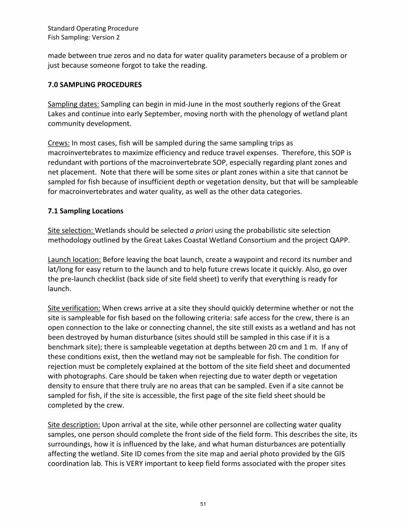
Standard Operating Procedure Fish Sampling: Version 2  

made between true zeros and no data for water quality parameters because of a problem or just because someone forgot to take the reading.    7.0 SAMPLING PROCEDURES  Sampling dates: Sampling can begin in mid‐June in the most southerly regions of the Great Lakes and continue into early September, moving north with the phenology of wetland plant community development.    Crews: In most cases, fish will be sampled during the same sampling trips as macroinvertebrates to maximize efficiency and reduce travel expenses.  Therefore, this SOP is redundant with portions of the macroinvertebrate SOP, especially regarding plant zones and net placement.  Note that there will be some sites or plant zones within a site that cannot be sampled for fish because of insufficient depth or vegetation density, but that will be sampleable for macroinvertebrates and water quality, as well as the other data categories.      7.1 Sampling Locations  Site selection: Wetlands should be selected a priori using the probabilistic site selection methodology outlined by the Great Lakes Coastal Wetland Consortium and the project QAPP.    Launch location: Before leaving the boat launch, create a waypoint and record its number and lat/long for easy return to the launch and to help future crews locate it quickly. Also, go over the pre‐launch checklist (back side of site field sheet) to verify that everything is ready for launch.   Site verification: When crews arrive at a site they should quickly determine whether or not the site is sampleable for fish based on the following criteria: safe access for the crew, there is an open connection to the lake or connecting channel, the site still exists as a wetland and has not been destroyed by human disturbance (sites should still be sampled in this case if it is a benchmark site); there is sampleable vegetation at depths between 20 cm and 1 m.  If any of these conditions exist, then the wetland may not be sampleable for fish. The condition for rejection must be completely explained at the bottom of the site field sheet and documented with photographs. Care should be taken when rejecting due to water depth or vegetation density to ensure that there truly are no areas that can be sampled. Even if a site cannot be sampled for fish, if the site is accessible, the first page of the site field sheet should be completed by the crew.   Site description: Upon arrival at the site, while other personnel are collecting water quality samples, one person should complete the front side of the field form. This describes the site, its surroundings, how it is influenced by the lake, and what human disturbances are potentially affecting the wetland. Site ID comes from the site map and aerial photo provided by the GIS coordination lab. This is VERY important to keep field forms associated with the proper sites 

51

Standard Operating Procedure Fish Sampling: Version 2  

and MUST appear on every page of the field sheets. Please also add crew names and identify the crew chief so everyone knows whom to ask if questions arise about a site.   

Shoreline structure: estimate the types of shoreline as percents for the site. Should sum to 100%. 

Nearshore landcover: estimate landcover that can be seen from your location in the wetland as a percent. Should sum to 100% (note that there is a spot for % that is not visable).  

Photos: take photos that illustrate the site and disturbances to it. Pictures of the shoreline can be particularly informative. Record digital photo numbers. 

Braiding index: For riverine systems, please select the appropriate braiding index from the list. Choose only one. NOTE: for riverine wetlands, also sketch a cross‐section of the wetland and river channel.  

Hydrologic connection: choose the description that best fits the wetland. Choose only one.  

Water level: select as many from the list as necessary to describe what is influencing the water level of the wetland on the day(s) that you are sampling.  

Habitat structure: select all habitats present in the wetland and then choose the most appropriate vegetation zone structure.  

Disturbances: circle all disturbances occurring within the site or within 250 m of its boundaries (use binoculars as necessary). Provide additional descriptions as requested on the field form. This information is very useful in interpreting invertebrate IBI scores; please fill it out carefully.  

On the back of the sheet, note weather conditions in the appropriate box. Update this as necessary throughout the sampling event. 

 Zones: Fish sampling is stratified by plant zone.  Three replicate fyke nets should be set in up to three monodominant vegetation zones that are of appropriate depth and meet the size requirements (see below).  Crews should sample up to three zones meeting the criteria below that are the most dominant in the wetland. Vegetation zones are patches of vegetation in which a particular plant type or growth form dominates the plant community based on visual coverage estimates.  Coverage of the dominant emergent or floating‐leaved form must be 75% or greater to qualify as a zone.  For example, a zone would be considered a Typha zone if the emergent+floating leaved vegetation was dominated (>75%) by Typha spp., even if submersed plants were found throughout the Typha spp. stand.  However, if a zone contains a mix of different emergent species/growth forms OR a mix of emergent and floating leaved species/growth forms, it should be avoided.  For example, if a stand contains both Nymphaea spp. (water lily) and Schoenoplectus spp. (bulrush) and neither of these plant types dominates (i.e., neither is >75% of the total emergent+floating leaved community), then the zone should be avoided.  Similarly, if a zone contains a mix of Schoenoplectus spp. and Peltandra virginica and neither plant type dominates the emergent+floating leaved community, then the area should be avoided.  In the case of SAV zones, there must be very little emergent (< 5 stems per m2) or floating leaved vegetation (< 1 stem per m2) mixed into the SAV for the zone to qualify as an SAV zone.  Note that other species or growth forms will likely occur sporadically within a 

52

Standard Operating Procedure Fish Sampling: Version 2  

given vegetation zone; however, the dominant plant type will be conspicuous if it exceeds 75% coverage.  Also note that zones are not necessarily a monodominant stand of just one species (e.g., Typha latifolia), but instead may be a morphotype (see the list of zones below).    Crews should draw on aerial photos of the site to indicate the location and size of vegetation zones, and to indicate fyke net locations.  A laser range finder should be used to determine the approximate size of the zone.  At least two measurements should be made along the long axis of the zone and at least two distances should be measured along the short axis of each zone.  The location of these measurements should be indicated with lines drawn on the aerial photo along with the distances.      Vegetation zones include (see abbreviations on field data sheet):  

Typha (cattail)  

Nuphar‐Nymphaea (water lily, combined) 

Schoenoplectus (bulrush; if there appear to be stem density differences in thick zones, use the distinctions below) 

o Inner Schoenoplectus: relatively‐dense inner zones along the shoreline that are protected from wave action by outer zones of vegetation.  

o Outer Schoenoplectus:  sparse outer zones where stem densities are lower than in inner zones due to wave action.  

Peltandra‐Sagittaria‐Pontederia (arrow‐arum‐arrowhead‐pickerel weed)  

Sparganium (bur‐reed)  

Wet meadow (mixed vegetation, typically Juncus and Eleocharis; if water ≥20 cm) 

Phragmites  

Submersed aquatic vegetation (SAV) 

Floating bog mat  

Open water (appropriate only for benchmark sites when a wetland has been degraded to the point that vegetation can no longer persist or if an area is being sampled to provide pre‐restoration information) 

Potentially other types if encountered.     Zone selection and size: Using an aerial photograph of the site, field crews should preliminarily identify vegetation zones. Upon arrival at the site, the crew leader should determine what vegetation zones can actually be sampled based on what is present in nearly monodominant stands with appropriate water depth of 20 cm to 1 m. This information should be sketched onto the aerial photo, showing how things have changed since the photograph was taken.  Minimum zone size is approximately 400 m2 so that nets can be separated by at least 20 m.  However, in cases where multiple disjointed smaller patches of the same vegetation type exist within a wetland, these smaller patches can each be sampled (1‐2 nets each) as long as the combined area exceeds approximately 400 m2 and no patch is smaller than approximately 100m2.  This strategy will most often be used in riverine wetlands where habitats are heterogeneous and plant patches tend to be small.    

53

Standard Operating Procedure Fish Sampling: Version 2  

 Depths: The depth range for fish sampling is 20‐100 cm.  Fyke net placement: Three replicate fyke nets are set in each inundated plant zone to provide a measure of variance associated with sampling.  Within each plant zone, each of the three replicate nets should be located at least 20 m from any other net to prevent the nets from interfering with one another. Spacing from one net to the next (i.e., between net 1 & 2 or 2 & 3) should not exceed 250 m in cases where the nets are set in the same patch. Note that macroinvertebrate sampling locations are associated with and adjacent to fyke net locations.  Water quality is also sampled in each plant zone.    Select the three fyke net locations to represent, to the degree possible, the variability in the plant zone.  In large plant zones, the three sampling points should correspond with different shoreline features if they occur and if this can be done under the spacing constraints mentioned above.  For example, in a large fringing wetland where the outer Schoenoplectus zone extends along the shoreline lakeward of a cottage, a forested area, and a wet meadow, sampling locations will be chosen to correspond with these different features. However, in many cases, a given vegetation zone will not cover enough area to be associated with different shoreline features, in which case sample locations should be chosen to represent, to the degree possible, the variability of the zone itself.  GPS waypoints should be created for each fyke net location.    7.2 Sample and Data Collection  Avoiding contamination of water quality samples: Since macroinvertebrates, fish, and water quality will all be sampled in each vegetation zone in very close proximity, field personnel should be very careful not to interfere with one another or compromise the other samples.  Every attempt should be made to collect water quality data and water samples first at each location before any movement is made around the point or zone.  When traveling to the site by boat, water quality data and water samples should be collected from the boat before anyone enters the water.  After water quality sampling, macroinvertebrate sampling and fish net deployment can commence.    Setting fyke nets: Fish communities are passively sampled by deploying fyke nets overnight at three locations each in up to three monodominant vegetation zones containing water of appropriate depth (20‐100 cm). Shallower or deeper water cannot be effectively fished with fyke nets of the dimensions listed in section 3.0. Thus, in complex wetlands, 9 nets will be set.   The small nets should be set in water approximately 20‐50 cm deep; larger nets are set in water depths of 50 – 100 cm.  The depth of water in each plant zone will dictate net size used since the main difference between large and small nets is height. The critical determinants are that the funnels are underwater and the opening frame is not overtopped.   

54

Standard Operating Procedure Fish Sampling: Version 2  

In dense vegetation or for small vegetation patches, nets should be placed perpendicular to the vegetation zone of interest, with leads extending from the center of the mouth of the net into the vegetation. Therefore, fishes in the plant zone or moving along the edge of the plant zone are likely to be caught. Wings should be set at 45° angles to the lead and connected to the outer opening on each side of the net.  In large plant zones, or less dense zones, nets should be set in the middle of the zone with the lead pointing toward shore.  Nets should be set so that the top of the cod end is far enough above the water surface to prevent turtles and other air breathing vertebrates from drowning. Nets should be set for one night (at least 12 hrs), and then checked.   Checking nets: Upon return to the nets, crews should first quickly look the net over to confirm that it appears to have remained upright, reasonably intact, and in the same condition as when the crew left. As the net is being pulled, any holes or other damage that might have affected net fishing integrity should be noted on field sheets. If the nets collapsed or had significant holes, crews must evaluate whether or not the zone was effectively “fished” (see re‐sampling below).   Crews should also be on the lookout for air‐breathing vertebrates that have been trapped. These should be either released as quickly as possible, or placed into a cooler or tub to revive, if necessary, before release.   Re‐sampling: Fish sampling is considered successful only if at least 2 of the 3 nets in each zone are determined to have “fished” for the night. This means that the nets remained upright without large holes or were otherwise compromised. If 2 of the 3 nets in a plant zone are determined by the field crew leader not to have representatively sampled the plant zone, that zone’s nets should be re‐set for a second night.  The senior field crew leader and/or the team’s PI should be consulted on this decision. If the fishing integrity of nets is not maintained for at least 2 of the 3 nets for a second night, the team’s PI must be consulted about whether to reset nets or move to the next site. In addition, if less than 10 fish are collected in total from all 3 nets within a plant zone, the nets should be re‐set for an additional night.    Fish processing: Fish should be identified to species, counted, measured, and released alive.  A minimum of 25 individuals per species and age category (2 categories: young‐of‐year [YOY] vs. older [i.e., not YOY]) will be measured to the nearest mm (total length [TL]). Fish smaller than 20 mm TL will not be counted or identified because fish this small are not accurately sampled by nets of our mesh size. When individuals are counted, separate tallies should be made for YOY vs. older individuals of each species. Any fish with external deformities (see list on field sheet) should be noted and photographed, if possible. All fish handling should follow university/governing agency wildlife use and care guidelines, and approved project‐specific plans should be in place at each institution before sampling begins. Appropriate state and provincial permits should also be obtained before sampling begins.    

55

Standard Operating Procedure Fish Sampling: Version 2  

Fish identification: All crews should have photo keys of Great Lakes fish species, including their key taxonomic characteristics. Such keys have been developed by Uzarski et al. (for GLCWC) and Brady et al. (for GLEI). If a fish cannot be identified in the field, representative specimens or high‐quality digital photographs should be returned to the laboratory for identification, with assistance from experts when necessary.   Euthanasia and preservation: Specimens being retained for a reference collection, ID confirmation in the laboratory (depending on fish size and state, provincial, and federal regulations), or those that have been severely injured during sampling should be humanely euthanized by over‐anesthetization, typically with MS‐222 mixed in the field to a concentration of 200 mg L‐1.  Clove oil (400‐600 mg L‐1) may also be used for fish euthanasia if approved by institutional and governmental agencies.  Crews should use the methods approved by their university’s IACUC committee or other governing body. The MS‐222 (or clove oil) solution should be prepared in a 5 gallon pail, or other suitable, well‐labeled container.  The container size should be large enough to easily contain the entire fish.  After euthanasia, fish should be preserved in 10% buffered formalin in a plastic, water‐tight bottle of appropriate size with internal and external water‐ and preservative‐proof labels (site ID, zone, fyke net number, unknown fish ID number, regional team code, and field crew leader name). Whenever unidentified fish specimens are kept, a note should be made on the field data sheets.  After use, the MS‐222 solution (or clove oil) should be flushed down the drain to a sanitary sewer with excess water.  If in a remote location where a sewer may not be readily available, further dilute the solution with water and dump wastes on land in a location away from water.  To dispose of euthanized fish (not preserved in ethanol or formalin), carcasses should be placed in two sealed plastic bags, frozen, and placed in a dumpster on the day of trash pick‐up for disposal in a licensed landfill.  Note that regulations or policies regarding MS‐222 or disposal of fish carcasses may vary by state/province, or institution.     For large specimens (>20 cm TL), or where collection of fish specimens is not allowed, fully‐ documented digital photographs will be collected instead of specimens.  When digital images are used, the species name (if known), site ID, plant zone, net number, date, number of specimens in the net, regional team code, and crew leader’s name will be included in the image.  Additional photographs of key features should be taken to aid identification of unknown specimens. Crews may find it advantageous to collect and archive a photograph of each different species encountered at a site.   7.3 Fish Reference Set  Laboratories should maintain a reference set of appropriately‐preserved specimens if allowed by state, provincial, or federal regulations.  Many regional laboratories already have reference collections of preserved specimens which can be used.  However, if species are encountered that are not part of the lab’s collection, a voucher specimen should be collected and preserved, 

56

Standard Operating Procedure Fish Sampling: Version 2  

if allowed.  For larger fish, high quality photographs may serve as “vouchers”, providing they are appropriately cataloged.   7.4 Additional Supplementary Data  Additional data to be collected at each replicate net include: latitude/longitude, vegetation percent coverage by growth form, plant zone size, organic sediment depth, mineral substrate texture, distance to depth zero (i.e., “shore”), and supplementary water quality data (if this hasn’t already been done by the macroinvertebrate crew; see the water quality SOP for details).    Sampling point locations: All sampling point locations should be recorded and stored using a handheld GPS receiver.  In case of GPS equipment failure, the crew should seek to borrow a GPS from another crew to finish the site, if possible, and should seek a replacement GPS unit. In the event that this is not possible, crews should endeavor to very accurately mark each fyke net location on their field map.  Macroinvertebrate sampling points may be close enough that separate GPS waypoints are not needed for nets; coordination with the macroinvertebrate crew is recommended.  Distance to depth 0: This is a distance‐to‐shore measurement to help determine bathymetric slope. Standing at the point at which depth has been recorded for the net, use a laser range finder to estimate the distance to depth 0, where the edge of the water is at the present time. Usually a member of the field crew will need to stand at the water’s edge so that the range finder has something to detect.  Vegetation quadrats: A 1‐m quadrat is used to determine vegetation percent coverage at fyke net locations.  The quadrat is placed at the mid‐point of the net lead on the right‐hand side when looking toward the open end of the net.  A ribbon or similar way of marking the midpoint of each lead is recommended.    Vegetation percent composition: Percent composition by growth form should be estimated visually within the quadrat.  Growth forms to be estimated are emergent, submergent, floating‐leaved, and include bare substrate. If species (or genera) within each growth form category are known, they should be noted on the field data sheet.  Although vegetation overlaps, the percentages should sum to 100%.    Zone/patch size: Crews should estimate the size of zones or the vegetation patches that comprise zones and note these on the fish data sheet. Range finders may be used to assist with this estimation. At least two measurements should be made along the long axis of the zone and at least two distances should be measured along the short axis of each zone.  The location of these measurements should be indicated with lines drawn on the aerial photo along with the distances.      

57

Standard Operating Procedure Fish Sampling: Version 2  

Organic substrate depth: Depth of organic substrate should be determined by pushing a 2‐cm diameter rod into the substrate until mineral substrates are reached. Placing the finger at this point of the substrate/water interface allows the rod to be withdrawn and the depth measured with a meter stick.   Mineral substrate texture: The dominant and subdominant mineral substrate type should be recorded. Mineral substrate texture is determined by feel using the categories and guidelines on the field data forms. This should be done at each net location.   Sediment samples:  Collection of sediment for %loss‐on‐ignition (%LOI) analysis is optional but highly recommended.  A 10‐cm deep sediment core should be collected using a piston corer or similar coring device.  Core diameter does not matter since samples will be homogenized for %LOI.  Sediment samples should be associated with each net location.  All samples from a given vegetation zone should be homogenized in a pail or tub using a hand trowel.  Approximately 100 ml (e.g., one trowel full) should be placed in a sealed container.  Samples may be stored in sealed plastic bags or plastic jars and fully labeled.  Samples should be stored on ice and then frozen.    Supplementary water quality data should be collected from each vegetation zone at the beginning of each sampling session. See the water quality SOP for detailed instructions.   Pictures: Crews should take digital images of each vegetation zone.  Any anomalies encountered or unique anthropogenic impacts should also be photo documented.  Digital images should be uploaded to a computer as soon as possible.  Photo file names should include, at a minimum, the site ID, date, and vegetation zone.  For photos of anomalies or disturbances, a word of description should be included in the file name.  Photos should be organized in directories labeled with site ID and sampling date.   8.0 SAMPLE HANDLING AND CUSTODY   Fish specimens should remain in the custody of field crews for the duration of each field trip. At the laboratory, unidentified fish specimens should be entered into the laboratory log‐in sheet, along with the date received and any notes about sample condition, and the information transferred to the sample processing inventory sheet. Specimens should be transferred to 70% ethanol after 2‐7 days in 10% buffered formalin. Preserved fish or their photographs (i.e., reference collections) should be stored for up to 5 years after collection in case there are further questions about proper identification.  9.0 EQUIPMENT TESTING, INSPECTION, and MAINTENANCE  Fyke nets will be examined for holes and defects before and after each net set. Crews should carry net repair kits with them and should repair nets in the field whenever possible. Major repairs may require the assistance of a net‐making company. Boat repairs are also often 

58

Standard Operating Procedure Fish Sampling: Version 2  

necessary. Most towns around the Great Lakes have boat repair shops, which can be used by field crews as necessary. However, crews should carry spare parts such as those listed in the equipment list.   All units that store files electronically should be backed up nightly to a laptop. This includes water quality meters, GPS units, cameras, and any other such equipment. This will help protect against massive data loss should equipment malfunction or be damaged or lost.  To prevent the spread of invasive species, including disease, boats and trailers will be drained and inspected upon haul‐out while still at the boat launch. All field gear, boats, and trailers will be drained, power‐washed or disinfected, and thoroughly dried before moving between sections of the Great Lakes (e.g., eastern vs. western Lake Erie, northern vs. southern Lake Michigan, etc.), and before moving between the lakes. No water will be transferred from one section of a Great Lake to another section or to an inland lake or water body.   GPS receivers will be tested prior to and after the field season by taking repeated readings at known localities, i.e., benchmarks.  All tests and results will be logged and the logs kept with the appropriate GPS units.  10.0 RECORD KEEPING/DATA ENTRY  Each field crew should carry with them maps and aerial photos of the sites to be visited, maps showing locations of the nearest boat launches, field data sheets for each scheduled site as well as spare datasheets, and a field notebook to document any additional information not contained on the field data sheet.  Each field data sheet should be initialed by the crew chief once a site is completed, and page 2 of the site‐level sheet requires the field crew chief’s signature.  Sample locations should be noted on the site map in the event that the GPS receiver is not functional.  Additional notes on anomalies or anthropogenic disturbances can also be made on the site map.  Documentation in the laboratory should include sample log‐in where unidentifiable specimens as well as voucher specimens to be added to reference collections will be logged.  All field data sheets as well as laboratory documentation are considered project records and should be archived for long term storage.  A supervising individual should initial each record prior to entering data into the data management system (DMS).  All records should be entered into the DMS as soon as possible.  Data collected in the field should be entered into the DMS immediately after returning from each field trip.  Fish identifications made in the laboratory should be noted on both the field data sheets as well as on the laboratory sheet and then entered into the DMS.  All data should be verified by a second person after it is entered into the DMS.  Field notes explaining anomalies, disturbances, etc. should also be entered into the DMS as soon as possible. All hard copy records (field data 

59

Standard Operating Procedure Fish Sampling: Version 2  

sheets, field notebooks, site maps with hand‐written notes, laboratory notebooks, etc.) should be compiled and stored in a secure location at each laboratory.   11.0 REFERENCES  Bailey, R.M., W.C. Latta, and G.R. Smith.  2004.  An atlas of Michigan fishes with keys and 

illustrations for their identification.  Miscellaneous Publications, Museum of Zoology, University of Michigan, Number 192. 

Cooper, M.J., C.R. Ruetz III, D.G. Uzarski and T.M. Burton. 2007. Distribution of round gobies (Neogobius melanostomus) in Lake Michigan drowned river mouth lakes and wetlands: do coastal wetlands provide refugia for native species? Journal of Great Lakes Research 33(2): 303‐313. 

Corkum, L. 2010. Fishes of Essex County and surrounding waters. Essex County Field Naturalists Club. 496pp. 

Hubbs, C.L., K.F. Lagler, and G.R. Smith.  2004.  Fishes of the Great Lakes region, Revised edition.  The University of Michigan Press. 

Murphy, B.R., and D.W. Willis, editors.  1996.  Fisheries techniques, 2nd edition.  American Fisheries Society, Bethesda, Maryland. 

Ruetz, C.R., III, D.G. Uzarski, D.M. Krueger, and E.S. Rutherford.  2007.  Sampling a littoral fish assemblage: comparing small‐mesh fyke nets and boat electrofishing.  North American Journal of Fisheries Management 27:825‐831. 

Uzarski, D.G., T.M. Burton, M.J. Cooper, J. Ingram, and S. Timmermans. 2005. Fish habitat use within and across wetland classes in coastal wetlands of the five Great Lakes: Development of a fish‐based Index of Biotic Integrity. Journal of Great Lakes Research 31(supplement 1): 171‐187. 

   12.0 FORMS  12.1  Field data sheet for fish and macroinvertebrates (attached) 

12.2  Field supplies/equipment checklist for fish and macroinvertebrate crews (attached) 

 

 

60

Information about these data sheetsLast updated March 2012Designed for use by Coastal Monitoring Fish and Invertebrate Field CrewsDesigned to be printed, then photocopied double-sided onto waterproof paperForm Site-Side 2 is a Word file, CM-fldchklist-Ver2Two copies of the Invert-WQ sheet should be printed to be photocopied back to back to allow for 4 zones per sheetOne double-sided fish sheet will be needed PER NET, so print MANY of these formsCrews only need a couple of copies of the codes-defs and Veg-list sheet (print these back to back and then laminate)

Notes for use:One copy of the site sheet (both sides) should be filled out per site. Use the checklist on the back to ensure everything gets done at a site.Water quality can be put on EITHER the invert sheet or the fish sheet (no need to duplicate). Check boxes allow indication of which sheet is used for WQ. This allows crew flexibilitySee the Fish and Invertebrate SOP for the detailed instructions on sampling sites.

61

Site Overview Datasheet version: 2Site ID: Site name (optional): Crew code: Sampling type: New(get info from map) Crew chief name: Finishing incomplete site

ShorelineShoreline Structure % of site Landcover near shore % of site GPS Unit No.:1. Sand Beach 1. Low Density Resid. Boat launch waypoint:2. Rocky Shoreline 2. High Density Resid. Boat launch lat:3. Cliff 3. Commercial/Indust Boat launch long: 4. RipRap 4. Ag5. Vegetated Bank 5. Upland forest6. Muddy Bank 6. Forested wetland7. Marsh 7. Marsh8. Other 8. Stream

9. OtherCan't see land (e.g.,cliff, hill)

Site morphometry & connectivitySketch cross-section of riverine sites

Braiding Index (riverine wtland only; select only one)0 channelized river1 unchannelized river, no meanders2 moderate meanders, no braiding3 multiple channels; no permanent vegetation4 multiple channels with permanent vegetation

Hydrologic connection to lake (select only one)0 strictly riverine connection to lake1 fully exposed to deep water portion of lake 2 fully exposed, but partially protected from direct wave action (e.g., submerged bar)

3 partially protected by sand bar, reef; opening is a large river 4 partially protected by sand bar, reef; opening is a small stream 5 fully separated from lake, but seasonal inundation possible6 fully separated from lake by permanent sand bar, dune, dyke

Water level (select as many as necessary)1 Water level stabilized by dyke2 Hydrology influenced by culvert, road3 Evidence of recent water level change (e.g., artificial dyke pumping)4 Evidence of long-term water level change (lake level)5 Weather-related current (onshore wind inducing seiche)6 Water level change not observed

WL comment: Habitat StructureHabitat Types (at scale of the entire wetland polygon) (circle all present)

riprap shallow emergent (shrubby) shallow emergent (herbaceous)bedrock floating leaf submergentboulder open water undercut bankcobble riverine / erosional riverine / depositionalsand wet meadow muddy / unvegetated shorelineorganic detritus island hummockmuck bog mat

Vegetation Zone Structure (choose only one)1 no vegetation2 zones by depth3 uniform distribution (e.g., single-species stand or even distribution of taxa all mixed together)4 patchwork mosaic (e.g., patches of cattail, bulrush, SAV, etc)

Disturbance (circle all present in site or within 250 m of site)RipRap Sewage Discharge Water Diversion Boat channels (#):Dredging (#) Industrial Discharge Channelization Mowing/veg removal (% of site):Marina Rec. docks (#): Ship docks (#): Shoreline Modification (describe below)

Shoreline modifications (describe):

Recreational activities: swimming sailing fishing motor-boating PWC

Pollution: Public Litter Commercial Refuse Petroleum Sewege Large Equipment Household Appliances

Evidence and location of other disturbance (incl. natural disturbance such as beaver, carp, muskrat) :

Site not sampleable for bugs or fish because….Acceptable reasons: no access, wetland no longer exists, water too deep/shallow, vegetation too dense (name it). Please describe below.

Photo #s

62

I verify that the datasheets for this site are complete and accurate: _______________________ (field crew chief signature)

Version 2 Site ID: Site Name: Date: Pre-launch Checklist: Calibrate meters ______________________ (signature) Notify DNR, others for sampling permission Nets intact, no holes

Download GPS points Download site information Upload GPS points to NRRI Update site information in site database

Crew names:

Field crew chief:

Weather (air temp, % cloud cover, wind (onshore, offshore, alongshore): Past 24 hr weather notes: Seiche evidence (onshore, offshore, none): Important reminders about this site: Site characterization form Invertebrate forms Fish forms Water Quality Photos of site Sketch of riverine site Boat launch GPS waypoint

Zones sampled (list): Zone: Zone: Zone: Zone:

Samples labeled Sediment characterization Water depth

Number of nets per zone: ____ Zone: ____ Zone: ____ Zone: ____ Zone: Fish length & anomalies Unidentified fish preserved &

labeled

Zones sampled (list): Zone: Zone: Zone: Zone:

In Situ WQ samples by: Zone Replicate

Overall site info Invertebrate Habitat Fyke net habitat Shoreline & landcover Site morphometry/hydrology Habitat & vegetation patches Disturbance and pollution River cross-section sketch

Plant quadrats Secchi depth/turbidity tube Sediment characterization

Plant quadrats Secchi depth/turbidity tube Sediment characterization

Notes: List broken equipment, supplies needed, notes for the next crew

63

Macroinvertebrate / Water Quality Field Data Sheet Crew code: Crew leader:

Date: Signature:Sheet______ of ________ for site

______Finishing incomplete site (check)Zone name (veg type)Start/end timeZone contiguous or in patches?Zone or patch size (m x m)Photos of zone

Replicate Number 1 2 3 1 2 3Latitude

Longitude

Waypoint ID

Depth (m)

Direction & dist to depth 0

% emergent

     dominant sp. or gen.

% floating leaved

     dominant sp. or gen.

% submergent

     dominant sp. or gen.

% bare substrate/open

Organic sed. depth (cm)

Substrate texture (dom/sub)

Number of 1 m net sweeps

Person‐minutes picking

Number of organisms

Vials per replicate

_____SEE FISH FORM FOR WQ DATA

In situ  water qualityDup. WQ (indicate rep)Transparency tube (cm)

Sample for % organic sed

WQ meter data file ID

Dissolved oxygen (mg/L)

DO % Saturation

Temperature (°C)

pH

Specific cond. (µS cm‐1)

Tot. Diss. Solids (g L‐1)†

Turbidity (NTU)

Redox pot. (mv)†

In situ  chloro. a (µg/L)†

Total Alk. (mg CaCO3 L‐1)

Pheno. Alk. (mg CaCO3 L‐1)

Sample volume prepped for storage

    Soluble reactive P

    NH4

    NO3

    Total P†

    Total N†

    Other:____________

Chlorophyll filter (y/n)

†=optional parameters

Notes:

Site ID:

64

Site ID: Sampling: initial reset Oriented (parallel/perp/angle): Crew code:

Site name (opt): Net-rep #: Date set: Unkn/Vouch Jars

Zone name (veg type): Fyke size: small large Time set: Collectors:Taxa (length in mm) 1 2 3 4 5 6 7 8 9 10 11 12 13 Comments

TLTL# Total

TLTL# Total

TLTL# Total

TLTL# Total

TLTL# Total

TLTL# Total

TLTL# Total

TLTL# Total

TLTL# Total

Anomalies: A=anchor worm B=black spot C=leeches D=deformities E=eroded fin F=fungus I=ich L=lesions N=blind P=parasites Y=popeye S=emaciated W=swirl scales T=tumor X=dead Z=other

Conditions: Net: twisted caught obstructed torn open disturbed Other : Water/Weather/Wind/Net Conditions:

Water depth at center post (m):Day 0 (m):_________ Day 1 (m): ____________

Date ck:

Time ck:

65

Taxa (length in mm) 1 2 3 4 5 6 7 8 9 10 11 12 13 CommentsTLTL# Total

TLTL# Total

TLTL# Total

TLTL# Total

TLTL# Total

TLTL# Total

TLTL# Total

General info Vegetation In situ Water QualityDepth (m): Direction & distance to depth 0: Quadrat: Temp (C) DO(%) pHGPS# Lat: Long: % emergent Scond(uS) DO(mg/L) Redox(mV)Veg Zone Zone or patch?      dominant sp. or gen. Temp C TDSZone or patch size (m x m) % floating leaved Turbidity (ntu) Chl aOrg sed depth (cm):      dominant sp. or gen. Tot Alk Pheno Alk

% submergent Meter data file ID: _____SEE BUG FORM FOR WQ DATA     dominant sp. or gen. Turb. Tube (cm)

% bare substrate/open

Sample Vol for lab WQ: SRP Substrate texture: 1 2 ____ Sample for %organic sed (optional)TP (opt) Notes: NO3

NH4

TN (opt)Other:____________Chlorophyll filter (y/n)

66

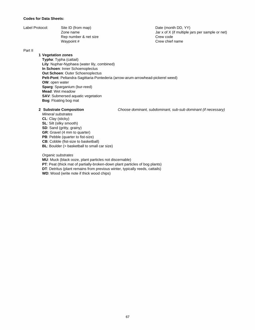
Codes for Data Sheets:

Label Protocol: Site ID (from map) Date (month DD, YY)Zone name Jar x of X (if multiple jars per sample or net)Rep number & net size Crew codeWaypoint # Crew chief name

Part II1 Vegetation zones

Typha: Typha (cattail) Lily: Nuphar-Nyphaea (water lily, combined)In Schoen: Inner SchoenoplectusOut Schoen: Outer SchoenoplectusPelt-Pont: Peltandra-Sagittaria-Pontederia (arrow-arum-arrowhead-pickerel weed)OW: open waterSparg: Sparganium (bur-reed)Mead: Wet meadowSAV: Submersed aquatic vegetationBog: Floating bog mat

2 Substrate Composition Choose dominant, subdominant, sub-sub dominant (if necessary)Mineral substratesCL: Clay (sticky)SL: Silt (silky smooth)SD: Sand (gritty, grainy)GR: Gravel (4 mm to quarter)PB: Pebble (quarter to fist-size)CB: Cobble (fist-size to basketball)BL: Boulder (> basketball to small car size)

Organic substratesMU: Muck (black ooze, plant particles not discernable)PT: Peat (thick mat of partially-broken-down plant particles of bog plants)DT: Detritus (plant remains from previous winter, typically reeds, cattails)WD: Wood (write note if thick wood chips)

67

Common Vegetation TaxaGenus Common Genus CommonAlisima Water Plantain Phalaris Canary Reed GrassBidens beckii Water Marigold Phragmites Cane GrassBrasenia schreberei Water Shield Pistia Water LettuceCalla Water Arum Pontederia PickerelweedCaltha Marsh Marigold Potamogeton Pond WeedCarex Sedge P. amplifoliusCeratophyllum Coon Tail P. crispusChara Water Cabbage P. natansEleocharis Spike Rush P. pectinatusElodea Water weed P. richardsoniiEquisetum Horse Tail Fern Ranunculus ButtercupHippuris Water Mare's Tail Sagittaria ArrowheadIris Iris (blue flag), yellow flag is non-native Schoenoplectus/Scirpus BulrushJuncus Rush Sium Water ParsnipLemna Duck Weed Sparganium sp. Bur ReedLythrum Loosestrife (purple loosestrife is non-native) Spiriodela Great Duck WeedMyriophyllum Water Milfoil Typha CattailNaias Bushy Pondweed Utricularia BladderwortNulumbo Lotus lily Vallisenaria Water CeleryNuphar Water Lily Zizania Wild RiceNymphaea Pond Lily

Fyke net problem codes:A: Depth: A1 too deep; A2 too shallow R: Rough surfB: Sediment: B1 unconsolidated; B2 rocky; B3 bedrock; B4 unsafe bog S: Size of site too smallD: Nets damaged or missing W: Weather not permittingH: No habitat available O: Other, please specifyM: Mechanical problems: M1 vehicle; M2 boat P: Permission lacking

Water quality problem codes:A: Depth: A2 too shallow O: Other; please specifyB: Sediment: B2 rocky; B3 bedrock; B4 unsafe bogM: Mechanical problems: M2 boat; M3 meters W: Weather not permitting

Invertebrate problem codes:A: Depth: A2 too shallowB: Sediment: B4 unsafe bog O: Other; please specifyN: Not done; explain on data sheet W: Weather not permitting

68

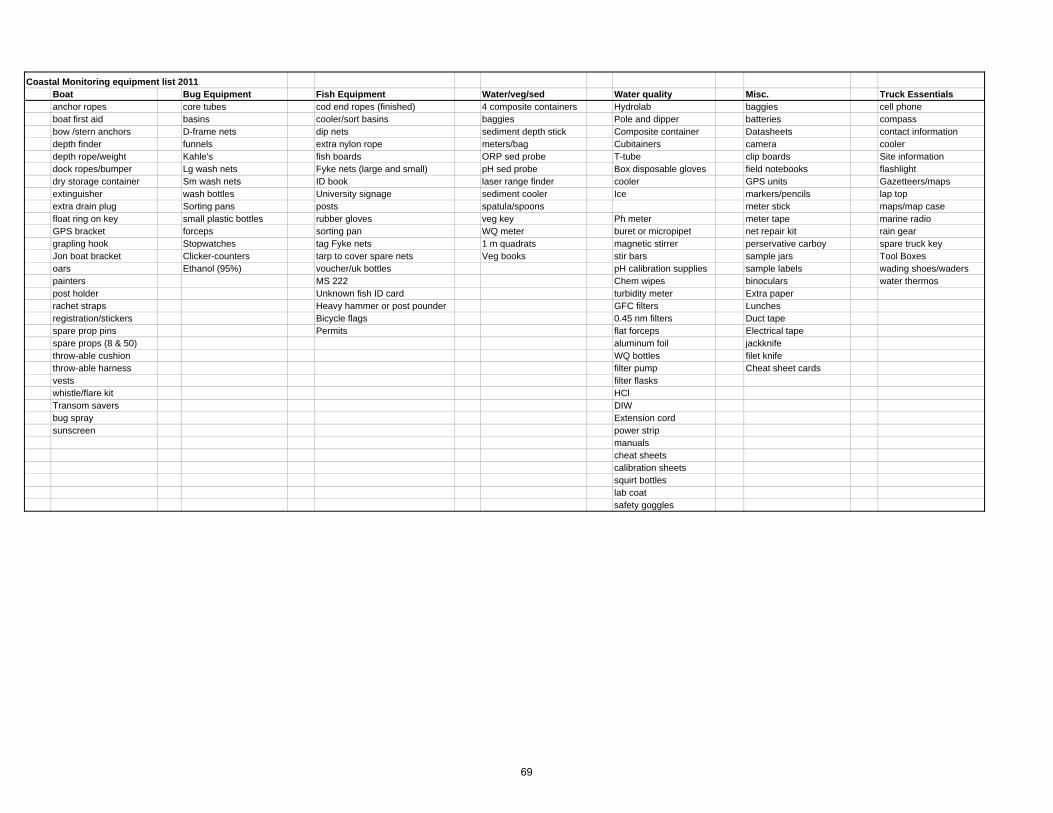
Coastal Monitoring equipment list 2011Boat Bug Equipment Fish Equipment Water/veg/sed Water quality Misc. Truck Essentialsanchor ropes core tubes cod end ropes (finished) 4 composite containers Hydrolab baggies cell phoneboat first aid basins cooler/sort basins baggies Pole and dipper batteries compassbow /stern anchors D-frame nets dip nets sediment depth stick Composite container Datasheets contact informationdepth finder funnels extra nylon rope meters/bag Cubitainers camera coolerdepth rope/weight Kahle's fish boards ORP sed probe T-tube clip boards Site informationdock ropes/bumper Lg wash nets Fyke nets (large and small) pH sed probe Box disposable gloves field notebooks flashlightdry storage container Sm wash nets ID book laser range finder cooler GPS units Gazetteers/mapsextinguisher wash bottles University signage sediment cooler Ice markers/pencils lap topextra drain plug Sorting pans posts spatula/spoons meter stick maps/map casefloat ring on key small plastic bottles rubber gloves veg key Ph meter meter tape marine radioGPS bracket forceps sorting pan WQ meter buret or micropipet net repair kit rain geargrapling hook Stopwatches tag Fyke nets 1 m quadrats magnetic stirrer perservative carboy spare truck keyJon boat bracket Clicker-counters tarp to cover spare nets Veg books stir bars sample jars Tool Boxesoars Ethanol (95%) voucher/uk bottles pH calibration supplies sample labels wading shoes/waderspainters MS 222 Chem wipes binoculars water thermospost holder Unknown fish ID card turbidity meter Extra paperrachet straps Heavy hammer or post pounder GFC filters Lunchesregistration/stickers Bicycle flags 0.45 nm filters Duct tapespare prop pins Permits flat forceps Electrical tapespare props (8 & 50) aluminum foil jackknifethrow-able cushion WQ bottles filet knifethrow-able harness filter pump Cheat sheet cardsvests filter flaskswhistle/flare kit HClTransom savers DIWbug spray Extension cordsunscreen power strip

manualscheat sheetscalibration sheetssquirt bottleslab coatsafety goggles

69

Standard Operating Procedure Macroinvertebrate Sampling and Laboratory Processing: Version 3  

       

Standard Operating Procedure  

Macroinvertebrate Sampling and Laboratory Processing   

Synopsis: A standardized method for collecting and processing macroinvertebrate samples according to Great Lakes Coastal Wetlands Consortium protocols for monitoring  

Great Lakes coastal wetlands.                     

Last updated March 2012   Contents:  

70

Standard Operating Procedure Macroinvertebrate Sampling and Laboratory Processing: Version 3  

1.0  PURPOSE……………………………………………………………………………………………………………………………3 2.0  RESPONSIBILITIES………………………………………………………………………………………………………………3 3.0  FIELD EQUIPMENT……………………………………………………………………………………………………….…….3 4.0  INSTRUMENT CALIBRATIONS AND FIELD PREPARATIONS……………………………………….……….5 5.0  BRIEF METHOD SUMMARY………………………………………………………………………………………………..6 6.0  SAMPLING PROCEDURES…………………………………………………………………………………………….…….6 

6.1  Sampling Locations…………………………………………………….………………….…………….………..6 6.2  Sample Collection…………………………………………………………………………..………………………9 6.3  Additional Supplementary Data………………………………………………………………..…..…….11 

7.0  SAMPLE HANDLING AND CUSTODY…………………………………………………………………………….……13 8.0  LABORATORY PROCESSING OF MACROINVERTEBRATE SAMPLES…………………………..……….13 

8.1  Laboratory Supplies/Equipment…………………………………………………………………….…….13 8.2  Sample Processing…………………………………………………………………………………………….....14 8.3  Laboratory Reference Set……………………………………………………………………………….…….15 

9.0  EQUIPMENT TESTING, INSPECTION, and MAINTENANCE……………………………………..…………16 10.0  RECORD KEEPING/DATA ENTRY…………………………………………………………………………..…….….16 11.0  REFERENCES…………………………………………………………………………………………………………..………17 

                       1.0 PURPOSE  

71

Standard Operating Procedure Macroinvertebrate Sampling and Laboratory Processing: Version 3  

The purpose of this Standard Operating Procedure (SOP) is to provide a standardized method for sampling and processing macroinvertebrates from Great Lakes coastal wetlands according to protocols developed by the Great Lakes Coastal Wetlands Consortium.  The methods described in this SOP describe how to accomplish macroinvertebrate sampling and sample processing by Great Lakes Coastal Wetland Monitoring Program protocols.  Index of Biotic Integrity (IBI) scores can be derived from data obtained using these methods.    2.0 RESPONSIBILITIES  Scientists and field teams sampling wetlands as part of a monitoring program following Great Lakes Coastal Wetland Consortium protocols should  ensure that all work performed satisfies the specific tasks and requirements outlined in this SOP and the project’s quality assurance project plan (QAPP).     All field and laboratory personnel performing macroinvertebrate sampling or laboratory processing as part of a monitoring program following Great Lakes Coastal Wetland Consortium protocols should follow this SOP and the project QAPP.  3.0 FIELD EQUIPMENT  D‐frame dip nets – Standard ‘D‐shaped’ macroinvertebrate sampling nets (approximate 26 cm wide) with 500‐µm mesh.  D‐shaped frame attached to long handle. Each crew should carry at least 2 nets at all times.  Gridded trays – 25‐cm x 30‐cm x 5‐cm deep (approximately) with 5x5‐cm gridlines drawn on the inside bottom of the trays. Trays should be light‐colored for ease of field‐picking invertebrates.  Forceps – various forceps for picking organisms from trays.  Include spares since they are frequently lost or damaged in the field.  Fine‐point forceps are generally preferred.     Stopwatch – at least one waterproof stopwatch per field crew.  Meter stick – at least one meter stick for measuring water depth.  1‐m square quadrat – PVC quadrat for estimating plant coverage.  Rod (approx. 2‐cm diameter x 1‐2 m) – rod is pushed into the sediment to determine organic/soft sediment depth.  Plastic or plastic‐coated garden stakes work well.  Global Positioning System (GPS) – each field crew will require at least one GPS.  Recreational‐quality GPS receivers are sufficient.  Also carry spare batteries or its charger. Heavily‐used GPS’s, or those with weak batteries, may require a mid‐day recharge. Adapters that connect to 12 v boat batteries are available and may be desired by crews. 

72

Standard Operating Procedure Macroinvertebrate Sampling and Laboratory Processing: Version 3  

 Laser range finder – a laser range finder is useful for measuring the distance to shore to estimate site slope, and for estimating the size of large vegetation zones. Spare batteries should also be carried.  Equipment/supply checklist – the checklist should be used before leaving on every field trip.  Field data sheets – pre‐printed waterproof data sheets for logging field data.  Printed site map – pre‐printed map on waterproof paper.  Field notebooks – waterproof notebooks or extra waterproof paper should be carried by each field crew to note any information not included in field datasheets.  Clipboard with storage compartment – all field sheets should be stored in a closeable clipboard or similar device.   Digital camera – for photo documentation of each site and any anomalies encountered. Spare batteries or the charging unit should also be carried.   Hand tally counters – a set of tally counters (one for each individual picking invertebrates).    Sample containers – 30‐ml or larger vials or jars for storing macroinvertebrate samples.  Glass screw‐top vials (approximately 25‐mm diameter x 95‐mm tall) with poly‐lined caps have been found to work well and are inexpensive.  A few additional larger jars should also be carried in the event that large invertebrates are collected.  Plastic vials/jars may also be used.  Internal sample labels – labels with pre‐printed fields for the various sample types.  Extra waterproof paper should also be carried for spare labels.  Sample container storage/transport system – a system to ensure sample containers remain organized and protected from breakage during transport.  Sediment coring device – 10‐cm deep sediment cores will be collected if sediment %loss on ignition (%LOI) is being determined.  This is an optional, though recommended, variable.  Coring devices are available for purchase, though a simple coring device can be made by sharpening the end of a piece of plastic pipe.  Core diameter does not matter since samples will be homogenized.  Trowel or similar device for mixing sediment – a garden trowel will be used to homogenize sediment if sediment samples are being collected for %LOI analysis.  

73

Standard Operating Procedure Macroinvertebrate Sampling and Laboratory Processing: Version 3  

Plastic bags for storing sediment – Zip top plastic bags should be used for storing sediment if samples are collected.  Alternatively, plastic jars may be used.  Plastic pail or tub for homogenizing sediment  Ethanol – 95% ethanol for preserving samples.    Personal equipment – field crews will need waders, appropriate outerwear, sunscreen, insect repellent, etc. for working in coastal wetlands.  All personnel should have a personal floatation device.  Binoculars – for navigation and for evaluating shoreline land use.  Boat/motor/trailer with all required safety and maintenance supplies and equipment – many sites will require navigation by boat.  A copy of this SOP – SOP should be printed on waterproof paper.  4.0 INSTRUMENT CALIBRATIONS AND FIELD PREPARATIONS  See the water quality SOP for water quality instrument calibrations.   GPS units: GPS receivers should be tested prior to and after the field season by taking repeated readings at known localities visible on aerial photographs or USGS benchmark locations.  During the field season, field crews should upload GPS readings regularly to their base GIS lab (in this case, the GIS laboratory at the Natural Resources Research Institute).  At least once per week, GIS personnel should plot GPS points onto aerial photographs of a sampled site and send the image to the field crew to verify that points appear to be reasonably accurate.  All tests and results should be logged and the logs kept with the appropriate GPS units.  D‐frame nets: D‐nets should be inspected for holes before and after each use. All small holes should be repaired with silicone. If nets contain large holes, nets should be swapped out with replacements until they can be patched.       5.0 BRIEF METHOD SUMMARY  Crews should collect macroinvertebrate samples from the major plant zones in each wetland during June through early September, with sampling dates targeting the appropriate phenology for the latitude. Sampling can begin earlier in the season in the most southerly parts of the 

74

Standard Operating Procedure Macroinvertebrate Sampling and Laboratory Processing: Version 3  

Great Lakes.  Preliminary identification of plant zones can be made from aerial photographs of each site (see zone definitions below), with confirmation or re‐adjustment made on‐site by field crew leaders based on the vegetation actually present at the time of sampling.  Samples are collected by sweeping vegetation with D‐nets, depositing net contents into gridded light‐colored trays, and then picking organisms from the trays.  Organisms are preserved in labeled vials of ethanol and later identified to genus (or operational taxonomic unit; see list) in the laboratory. IBI scores can be calculated from these data.  Sampling methodology is based on Burton et al. (1999), Uzarski et al. (2004), Cooper et al. (2006), and Cooper et al. (2007).  It is very important that ALL fields on the field data sheets are completed appropriately. Blank fields cannot be properly interpreted. If data cannot be collected, this should be noted with the appropriate error code. Crews should also be aware that there is a large difference between a zero and “no data”. It is especially problematic when no distinction is made between true zeros and no data for water quality parameters because of a problem or just because someone forgot to take the reading.    6.0 SAMPLING PROCEDURES  Sampling dates: Sampling can begin in mid‐June in the most southerly regions of the Great Lakes and continue into early September, moving north with the phenology of wetland plant and macroinvertebrate communities.    Crews: In most cases, macroinvertebrates will be sampled during the same sampling trips as fish to maximize efficiency and reduce travel expenses.  Therefore, this SOP makes references to the other sampling events to show how sampling is connected/coordinated.  Note that there will be some sites or plant zones within a site that cannot be sampled for fish because of insufficient depth, but that will be sampleable for macroinvertebrates and water quality, as well as the other data types.  6.1 Sampling Locations  Site selection: Wetlands should be selected a priori using the probabilistic site selection methodology outlined by the Great Lakes Coastal Wetland Consortium and the project QAPP.    Launch location: Before leaving the boat launch, create a waypoint and record its number and lat/long for easy return to the launch and to help future crews locate it quickly. Also, go over the pre‐launch checklist (back side of site field sheet) to verify that everything is ready for launch.   Site verification: When crews arrive at a site they should quickly determine whether or not the site is sampleable for macroinvertebrates. For GLCWC‐type monitoring protocols, the criteria are: safe access for the crew, wetland still exists as a wetland with aquatic vegetation, the site is connected to a Great Lake or major connecting channel (e.g., St. Mary’s River), and there is 

75

Standard Operating Procedure Macroinvertebrate Sampling and Laboratory Processing: Version 3  

sampleable vegetation at depths between 5 cm and 1 m. If any of these conditions exist, then the wetland may not be sampleable for macroinvertebrates. The condition for rejecting a site must be completely explained at the bottom of the site field sheet and documented with photographs. Care should be taken when rejecting due to water depth or vegetation to ensure that there truly are no areas that can be sampled. Even if a site cannot be sampled for macroinvertebrates, if the site is accessible, the first page of the site field sheet should be completed by the crew.   Site description: Upon arrival at the site, while other personnel are collecting water quality samples, one person should complete the front side of the site field form. This describes the site, its surroundings, how it is influenced by the lake, and what human disturbances are potentially affecting the wetland. Site ID comes from the site map and aerial photo provided by the GIS coordination lab. This is VERY important to keep field forms associated with the proper sites and MUST appear on every page of the field sheets. Please also add crew names and identify the crew chief so everyone knows whom to ask if questions arise about a site.  

Shoreline structure: estimate the types of shoreline as percents for the site. Should sum to 100%. 

Nearshore landcover: estimate landcover that can be seen from your location in the wetland as a percent. Should sum to 100% (note that there is a spot for % that is not visable).  

Photos: take photos that illustrate the site and disturbances to it. Pictures of the shoreline can be particularly informative. Record digital photo numbers. 

Braiding index: For riverine systems, please select the appropriate braiding index from the list. Choose only one. NOTE: for riverine wetlands, also sketch a cross‐section of the wetland and river channel.  

Hydrologic connection: choose the description that best fits the wetland. Choose only one.  

Water level: select as many from the list as necessary to describe what is influencing the water level of the wetland on the day(s) that you are sampling.  

Habitat structure: select all habitats present in the wetland and then choose the most appropriate vegetation zone structure.  

Disturbances: circle all disturbances occurring within the site or within 250 m of its boundaries (use binoculars as necessary). Provide additional descriptions as requested on the field form. This information is very useful in interpreting invertebrate IBI scores; please fill it out carefully.  

On the back of the sheet, note weather conditions in the appropriate box. Update this as necessary throughout the sampling event. 

 Zones: Macroinvertebrate sampling is stratified by plant zone.  Three replicate macroinvertebrate samples should be collected from up to 4 monodominant vegetation zones that are of appropriate depth and meet the size requirements (see below). If there are more than 4 zones, crews should sample the vegetation zones that are the most dominant in the wetland. Crews should draw on the aerial photos of the sites to indicate location and size of vegetation zones, and should also indicate locations of sampling points. Vegetation zones are 

76

Standard Operating Procedure Macroinvertebrate Sampling and Laboratory Processing: Version 3  

patches of vegetation in which a particular plant type or growth form dominates the plant community based on visual coverage estimates.  Coverage of the dominant emergent or floating leaved form must be 75% or greater to qualify as a zone.  For example, a zone would be considered a Typha zone if the emergent+floating leaved vegetation was dominated (>75%) by Typha spp., even if submersed plants were found throughout the Typha spp. stand.  However, if a zone contains a mix of different emergent species/growth forms OR a mix of emergent and floating leaved species/growth forms, it should be avoided.  For example, if a stand contains both Nymphaea spp. (water lily) and Schoenoplectus spp. (bulrush) and neither of these plant types dominates (i.e., neither is >75% of the total emergent+floating leaved community), then the zone should be avoided.  Similarly, if a zone contains a mix of Schoenoplectus spp. and Peltandra virginica and neither plant type dominates the emergent+floating leaved community, then the area should be avoided.  In the case of SAV zones, there must be very little emergent (< 5 stems per m2) or floating leaved vegetation (< 1 stem per m2) mixed into the SAV for the zone to qualify as an SAV zone.  Note that other species or growth forms will likely occur sporadically within a given vegetation zone; however, the dominant plant type will be conspicuous if it exceeds 75% coverage.  Also note that zones are not necessarily a monodominant stand of just one species (e.g., Typha latifolia), but instead may be a morphotype (see the list of zones below).    A laser range finder should be used to determine the approximate size of the vegetation zone.  At least two measurements should be made along the long axis of the zone and at least two distances should be measured along the short axis of each zone.  The location of these measurements should be indicated with lines drawn on the aerial photo along with the distances.     Vegetation zones include (see abbreviations on field data sheet):  

Typha (cattail)  

Nuphar‐Nymphaea (water lily, combined) 

Schoenoplectus (bulrush; if there appear to be stem density differences in thick zones, use the distinctions below) 

o Inner Schoenoplectus: relatively‐dense inner zones along the shoreline that are protected from wave action by outer zones of vegetation.  

o Outer Schoenoplectus:  sparse outer zones where stem densities are lower than in inner zones due to wave action.  

Peltandra‐Sagittaria‐Pontederia (arrow‐arum‐arrowhead‐pickerel weed)  

Sparganium (bur‐reed)  

wet meadow (mixed vegetation, typically Juncus and Eleocharis) 

Phragmites  

Submersed aquatic vegetation (SAV) 

Floating bog mat  

Open water (appropriate only for benchmark sites when a wetland has been degraded to the point that vegetation can no longer persist or if an area is being sampled to provide pre‐restoration information) 

77

Standard Operating Procedure Macroinvertebrate Sampling and Laboratory Processing: Version 3  

Potentially other types if encountered.     Zone selection and size: Using an aerial photograph of the site, field crews should preliminarily identify vegetation zones. Upon arrival at the site, the crew leader should determine what vegetation zones can actually be sampled based on what is present in nearly monodominant stands with appropriate water depth of 5 cm to 1 m. This information should be sketched onto the aerial photo, showing how things have changed since the photograph was taken.  Minimum zone size is approximately 400 m2), so that replicates can be separated by at least 15 m.  However, in cases where multiple disjointed smaller patches of the same vegetation type exist within a wetland, these smaller patches can each be sampled (1 or 2 replicates each) as long as the combined area exceeds approximately 400 m2 and no patch is smaller than 25m2.  If there are enough disjunct patches for a choice to be made by the field crew, the larger patches should be sampled. This strategy will most often be used in riverine wetlands where habitats are heterogeneous and plant patches tend to be small.     Depths: The minimum depth for sampling macroinvertebrates is 5 cm and the maximum depth is 1 m.      Replicate placement in zones: Three replicate dip net samples should be collected in each inundated vegetation zone to provide a measure of variance associated with sampling.  These replicates should be at least 15 m apart, and should be associated with and adjacent to fish fyke net locations if fish are also being sampled in that zone.  Spacing from one replicate sample location to the next (i.e., between replicates 1 & 2 or 2 & 3) should not exceed 250 m in cases where the samples are collected in the same patch.    Select the three sampling points to represent the variability in the vegetation zone.  In large vegetation zones, the three sampling points should correspond with different shoreline features if they occur and if this can be done under the spacing constraints mentioned above.  For example, in a large lacustrine wetland where the outer Schoenoplectus zone extends along the shoreline lakeward of a cottage, a forested area, and a wet meadow, sampling locations will be chosen to correspond with these different features. However, in many (or most) cases, a given vegetation zone will not cover enough area to be associated with different shoreline features, in which case sample locations should be chosen to represent, to the degree possible, the variability of the zone itself.    6.2 Sample Collection  Avoiding contamination of water quality samples: Since macroinvertebrates, fish (when possible), and water quality will all be sampled in each vegetation zone, field personnel should be very careful not to interfere with one another or compromise the other samples.  Every attempt should be made to collect water quality data and water samples first at each location before any movement is made around the point or zone.  When traveling to the site by boat, 

78

Standard Operating Procedure Macroinvertebrate Sampling and Laboratory Processing: Version 3  

water quality data and water samples should be collected from the boat before anyone enters the water.  After water quality sampling, macroinvertebrate sampling and fish net deployment can commence.    Dip‐netting macroinvertebrates:  Each dip net replicate consists of a composite of sweeps taken at the surface, mid‐depth, and at the water‐sediment interface while brushing vegetation with the net to incorporate all microhabitats at a given replicate sampling point.  Care should be taken not to collect excessive amounts of sediment, which will make field‐picking of organisms difficult. However, many organisms live at the water‐sediment interface, so the sediment needs to be gently “beaten” with the bottom of the net to dislodge organisms up into the water column where they can be captured.    To semi‐quantify sampling effort, the number of net sweeps (i.e., 1 to 2‐m passes) should be counted and recorded on the sampling data sheet for each replicate sample.  After a series of net sweeps is made, the net will contain an assortment of invertebrates, detritus, and vegetation fragments.  Net contents can then be emptied into gridded, light‐colored pans.    Field‐picking: Samples need to be picked while still at each sample location in case more net sweeps are required to reach the target number of organisms. Net contents should be distributed evenly across each pan prior to picking organisms.  The person doing the netting should continue to sample and fill the pan(s) until a sufficient number of organisms has been collected to begin field picking, at which time the number of net sweeps will be recorded on the data sheet.  The number of net sweeps required depends on macroinvertebrate densities in each zone. For example, in zones replete with macroinvertebrates, only 5‐10 net sweeps are required to fill pans, while in zones with sparse macroinvertebrate communities, many more sweeps will need to be made before picking can begin.   Avoid adding excessive amounts of vegetation and detritus to pans because this will significantly reduce picking efficiency.  A maximum of approximately 75% of the pan surface area should be covered by vegetation and detritus, leaving at least 25% of the pan bottom uncovered in order to see the grid lines.  Only a small amount of water (2‐5 mm depth) is needed to facilitate picking of swimming organisms.   When possible, multiple individuals should work together to collect each replicate sample.  They can either work from the same pan or work from separate pans, or a combination (e.g., 2 individuals working from one pan while one individual works from a different pan) and place organisms into a single vial for that replicate sample.  The picking target is 150 macroinvertebrates for each replicate from each zone. Macroinvertebrates should be collected using forceps (no other picking tools are allowed), with individuals working systematically from one end of the pan to the other, attempting to pick all specimens from each grid cell before moving on to the next. No other picking tools besides forceps are allowed because this alters the bias of which invertebrates are picked from the pan. Special efforts should be made to ensure that smaller, cryptic, and/or sessile organisms (those resting on or attached to 

79

Standard Operating Procedure Macroinvertebrate Sampling and Laboratory Processing: Version 3  

vegetation or debris) are not overlooked within each grid square. Hand‐tally counters should be used to keep track of how many organisms are collected.  In the absence of hand‐tally counters, individuals working on the same sample should count out loud to ensure that the target number of organisms is collected.    Picking time: In most cases, 150 organisms per replicate can be obtained within ½‐person‐hour, the time limit for the first picking. Picking of individual replicates should be timed using a stopwatch.  If 150 organisms are picked before ½ person‐hour (i.e., two people for 15 minutes; three people for 10 minutes, etc.) elapses, then picking stops at 150 and the number of person‐minutes is recorded on the data sheet.  If 150 organisms are not acquired within ½ person‐hour, the clock should be stopped, organisms are tallied, and the running clock will resume as picking continues to the next multiple of 50, regardless of the time required to do so. For example, if after ½ person‐hour 115 organisms have been collected, then picking will continue to 150, regardless of how long it takes to do so. Therefore, each replicate sample should contain 50, 100, or 150 organisms.  After each replicate sample is picked, the total number of person‐minutes required for collection, as well as the number of organisms collected, should be recorded on the data sheet.  It is important to reduce picking bias.  Accordingly, the number of organisms remaining in each of the picked grids should nearly always be exhausted to the point where finding just a few more organisms will require a substantial effort. Only then should the next grid square be picked. If the entire pan is ‘picked clean’ before the target number of specimens is reached, then timing should stop while dip nets are used to refill the pan(s).    Preservation: Macroinvertebrates should be immediately placed into labeled 30‐ml or larger leak‐proof vials containing 95% ethanol.  Sample containers should be labeled with both internal and external labels. External labels should only be those that have previously been checked for ability to remain adhered to sample bottles even when wet. They should be written on with black fine point Sharpie markers or similar markers that have been tested and proven to be waterproof. Internal labels should be made from waterproof paper and written on with either waterproof ink or pencil.  Labels should include site ID, vegetation zone, replicate number, sample date, and crew chief name (see labeling protocol on field data sheets).  If more than one vial is needed for a replicate sample, each should be labeled separately and numbered (e.g., 1 of 2, 2 of 2, etc.). If glass sample vials are used, they must be stored in a manner that prevents breakage during transport.  6.3 Additional Supplementary Data  Additional data to be collected with each macroinvertebrate replicate sample include: latitude/longitude, vegetation percent cover by growth form, organic substrate depth, mineral substrate texture, and supplementary water quality data (see water quality SOP).    

80

Standard Operating Procedure Macroinvertebrate Sampling and Laboratory Processing: Version 3  

Sampling point locations: All sampling point locations should be recorded and stored using a handheld GPS receiver.  In case of GPS equipment failure, the invertebrate crew should seek to borrow a GPS from another crew to finish the site, if possible, and should seek a replacement GPS unit. In the event that this is not possible, crews should endeavor to very accurately mark each sample point on their field map.    Vegetation quadrats: A 1‐m2 quadrat is used to determine vegetation percent coverage at fish and macroinvertebrate sampling points.  If both fish and macroinvertebrates are being sampled, the quadrat should be placed at the mid‐point of the net lead on the right‐hand side when looking toward the open end of the net.  A ribbon or similar way of marking the midpoint of each lead is recommended.  In locations where fish are not being sampled, quadrats should be placed roughly in the center of the area where dip net sweeps were made.  To randomize the specific location these quadrats, quadrats should be thrown over the individual’s shoulder to reduce bias in sampling location.    Vegetation percent composition: Percent composition by growth form should be estimated visually within the quadrat.  Growth forms to be estimated are emergent, submergent, floating leaved, and include bare substrate. If species (or genera) within each growth form category are known, they should be noted on the field data sheet.  Although vegetation overlaps, the percentages should sum to 100%.    Zone/patch size: Crews should estimate the size of zones or the vegetation patches that comprise zones and note these on the fish data sheet. Range finders may be used to assist with this estimation. At least two measurements should be made along the long axis of the zone and at least two distances should be measured along the short axis of each zone.  The location of these measurements should be indicated with lines drawn on the aerial photo along with the distances.      Organic substrate depth: Depth of organic substrate should be determined by pushing a 2‐cm diameter rod into the substrate until mineral substrates are reached. Placing the finger at this point of the substrate/water interface allows the rod to be withdrawn and the depth measured with a meter stick.   Mineral substrate texture: The dominant and subdominant mineral substrate type should be recorded. Mineral substrate texture is determined by feel using the categories and guidelines on the field data forms. This should be done at each D‐net sampling location.   Sediment samples:  Collection of sediment for %loss‐on‐ignition (%LOI) analysis is optional but highly recommended.  A 10‐cm deep sediment core should be collected using a piston corer or similar coring device.  Core diameter does not matter since samples will be homogenized for %LOI.  Sediment samples should be associated with each net location if fish are being sampled or the center of dip‐netting area if fish are net being sampled.  All samples from a given vegetation zone should be homogenized in a pail or tub using a hand trowel.  Approximately 

81

Standard Operating Procedure Macroinvertebrate Sampling and Laboratory Processing: Version 3  

100 ml (e.g., one trowel full) should be placed in a sealed container.  Samples may be stored in sealed plastic bags or plastic jars and fully labeled.  Samples should be stored on ice and then frozen.    Supplementary water quality data should be collected from each vegetation zone at the beginning of each sampling session. See the water quality SOP for detailed instructions.   Pictures: Crews should take a digital picture of each vegetation zone.  For sites, any anomalies encountered or unique anthropogenic impacts should also be photo documented.  Digital images should be uploaded to a computer as soon as possible after each sampling trip.  Photo file names should include, at a minimum, the site ID and vegetation zone.  For photos of anomalies or disturbances, a word of description should be included in the file name.  Photos should be organized in directories labeled with site ID and sampling date.   Site completion: Before leaving the site, use the checklist on the back side of the site sheet to verify that everything has been completed. The field crew leader must sign this sheet at the bottom to verify that the site has been completely sampled to the best of the crews’ ability, and that all information on the field forms is accurate and complete.    7.0 SAMPLE HANDLING AND CUSTODY  Samples should remain in the custody of field crews for the duration of each field trip. At the laboratory, each sample should be logged into the laboratory log book.  Entries should include: site ID, plant zone, replicate number, and sample date, along with the date received and any notes about sample condition. This information should be transferred to a sample processing inventory maintained by each laboratory. This inventory should be updated as each sample is processed. Processed samples should remain in the custody of the laboratory. Identified macroinvertebrates should be stored for 5 years after collection. Invertebrate identifications should be compiled in laboratory notebooks, and then entered into the data management system. The hard‐copy field data sheets and laboratory notebooks should be stored at each regional laboratory.  8.0 LABORATORY PROCESSING OF MACROINVERTEBRATE SAMPLES  8.1 Laboratory Supplies/Equipment  Sample log‐in notebook – a notebook or spreadsheet to log samples into the laboratory.  Sample inventory sheet – a sheet that identifies the exact stage of processing for every sample housed in the laboratory and identifies the individual working on the sample at that stage.  

82

Standard Operating Procedure Macroinvertebrate Sampling and Laboratory Processing: Version 3  

Identification sheets –laboratory notebooks or data sheets for keeping records of macroinvertebrate specimen IDs and counts.    Forceps – various forceps for manipulating organisms under magnification.    Petri dishes, watch glasses or similar containers – small clear dishes for processing invertebrate samples under microscopes and for temporarily storing samples while processing.  Ethanol – 95% ethanol for preserving samples.    Dissecting microscopes – stereo microscopes (at least some of which are capable of 50x or greater magnification) with appropriate light source for identifying macroinvertebrates in the laboratory.    Small storage vials – 5‐15‐ml (approximate) storage vials for long term storage of macroinvertebrate samples.  Vials must have appropriate caps to prevent ethanol from evaporating over time.  Poly‐lined caps have been found to work well.    Vial storage system – A storage system such as vial trays stored in a cabinet is necessary to keep archived samples organized.  Taxonomic keys – an appropriate set of taxonomic keys for identifying macroinvertebrates to genus level (see list below).       

83

Standard Operating Procedure Macroinvertebrate Sampling and Laboratory Processing: Version 3  

8.2 Sample Processing  Strict inventory control of macroinvertebrate samples must be maintained since each laboratory will likely have multiple individuals working on various aspects of sample processing.  Sample inventory sheets will be used to track every aspect of sample processing.  Fields within inventory sheets will contain actions such as ‘Sample Received by Laboratory,’ ‘Initial Processing to Family,’ ‘Gastropods Processed to Genus,’ ‘Insects Processed to Genus,’ ‘All Data Entered Into Database,’ etc.  Inventory sheets will be designed to track who is working on each action listed and will include space for individuals to sign when an action is completed.  At a minimum, a quality control auditor should be able to easily determine the location and progress of any macroinvertebrate sample in the custody of the regional laboratory.  For macroinvertebrate identification, taxonomic keys listed in the “Levels of Identification and Other Taxa Notes” working document should be used (see attached). This document also shows the target lowest operational taxonomic unit for each group. This is typically genus for insects. However, chironomid larvae need only be identified to tribe or subfamily (e.g., Chironomini, Tanytarsini, Tanypodini, etc.) for the GLCWC IBI calculations.  Specimen IDs and counts should be recorded along with the following information: date(s) that the sample is being worked on, site ID, vegetation zone, replicate number, and sample processer’s name.   Any difficulties encountered during identification (e.g., missing gills) should also be noted.  Taxa identification and specimen counts are considered a ‘laboratory record’ so identification sheets should be archived accordingly.    In most cases, identified organisms will be placed into smaller vials (e.g., 5‐15 ml) for archiving.  Each laboratory must develop a system for archiving samples that allows later taxonomic verification and QA/QC.  For taxonomic groups with many individuals, vials for archiving samples may contain specimens at the family (i.e., one family per vial) or order level.  Discretion must be used when determining the taxonomic level at which samples are stored.  Some regional laboratories may choose to archive samples at either a higher taxonomic level (e.g., class) or store entire processed replicate samples together.    Vials should be filled with 70‐95% ethanol for long‐term storage.  Labels containing the site ID, vegetation zone, replicate number, taxonomic identification, and sample processer’s initials should be included within each vial.  Vials should be organized in containers such as plastic or cardboard trays labeled with all pertinent sample information and stored in a secure location.  Ethanol levels should be inspected periodically to prevent dessication of archived samples.    Active communication among teams is essential to consistent taxonomy.  Individuals who are processing macroinvertebrate samples should use a variety of techniques to communicate with other teams while working through particularly difficult identifications.  E‐mail and phone calls as well as an online forum where photos can be posted will all be used to aid macroinvertebrate processing and ensure accuracy.  As new technicians are trained in 

84

Standard Operating Procedure Macroinvertebrate Sampling and Laboratory Processing: Version 3  

laboratory processing of macroinvertebrates, they will also receive training on how to best communicate with other project participants working on macroinvertebrate processing.  8.3 Laboratory Reference Set  Each laboratory should develop a reference set of preserved specimens that will include at least 3 individuals (when possible) of each taxon.  This reference set can be used to train new individuals and for cross‐laboratory taxonomic verification.  Specimens that are removed from their respective sample vials to be included in the reference set will be replaced with a label indicating that the specimen(s) was moved to the reference set; this should also be noted on the data sheet. Labels within the vials in the reference set must contain all relevant information for where the specimen came from (site ID, vegetation zone, replicate number, taxonomic identification, and sample processer’s initials).  Care must be taken to ensure that each individual specimen contained in the reference set is linked back to the appropriate sample that it came from.  For example, if three specimens represent a given taxon within the reference set and are all contained within the same reference set vial, they should have all come from the same original sample.  Alternatively, if individual specimens for a given taxon in the reference set came from different samples, they must be contained in separate labeled vials so that each specimen can be linked back to the appropriate sample.  9.0 EQUIPMENT TESTING, INSPECTION, and MAINTENANCE  D‐frame nets will be inspected before and after each set of sample collections for holes or other damage. Damaged nets will be repaired in the field, and replaced at the end of that sampling trip.  Each crew will have one replacement net with them at all times. Crews should also carry extra forceps and hand tally counters. Boat repairs are also often necessary. Most towns around the Great Lakes have boat repair shops, which will be used by field crews as necessary. Spare parts carried by crews will include spark plugs and appropriate wrenches, tire for the trailer, drain plug, fuel line, sheer pins (if used), and a spare propeller. Spare batteries will be carried for the GPS units, cameras, and water quality meters.   All units that store files electronically should be backed up nightly to a laptop. This includes water quality meters, GPS units, cameras, and any other such equipment. This will help protect against massive data loss should equipment malfunction or be damaged or lost.   Boats, trailers, and sampling gear must undergo rigorous disinfection to eliminate the transfer of exotic species between sections of the Great Lakes (e.g., eastern vs. western Lake Erie, northern vs. southern Lake Michigan, etc), and before moving between the lakes. This means that all boats, trailers, and gear need to be washed well, preferably through a car wash, before moving the gear between sections of the Great Lakes.    10.0 RECORD KEEPING/DATA ENTRY 

85

Standard Operating Procedure Macroinvertebrate Sampling and Laboratory Processing: Version 3  

 Each field crew should carry with them maps and aerial photos of the sites to be visited, maps showing locations of the nearest boat launches, field data sheets for each scheduled site as well as spare datasheets, and a field notebook to document any additional information not contained on the field data sheet.  Each field data sheet should be initialed by the crew chief once a site is completed, and page 2 of the site‐level sheet requires the field crew chief’s signature.  Sample locations should be noted on the site map in the event that the GPS receiver is not functional.  Additional notes on anomalies or anthropogenic disturbances can also be made on the site map.  Documentation in the laboratory will include sample log‐in, sample inventory sheets, and identification sheets on which macroinvertebrate processing and identification records are kept.  When multiple individuals are working on the same sample, data should be compiled into a single record for the sample.  A supervising individual should initial the record prior to the data being entered into the data management system (DMS).  A separate identification record should be kept for the macroinvertebrate reference set that includes the taxonomic ID, site ID, vegetation zone, replicate number, sample date, and the individual who identified the organism.  This is the same information to be included on the internal labels for each vial in the reference set.  All records should be entered into the DMS as soon as possible.  Data collected in the field should be entered into the DMS immediately after returning from each field trip.  All data will be verified by a second person after it is entered into the DMS.  Field notes explaining anomalies, disturbances, etc. will also be entered into the DMS.  After completing laboratory processing of each replicate invertebrate sample, data will be entered into the DMS and verified by a second individual.  All hard copy records (field data sheets, field notebooks, site maps with hand‐written notes, sample inventories, laboratory notebooks with macroinvertebrate IDs, etc.) should be compiled and stored in a secure location at each laboratory.  

11.0 REFERENCES  Burton, T.M., D.G. Uzarski, J.P. Gathman. J.A. Genet, B.E. Keas, and C.A. Stricker. 1999.  

Development of a preliminary invertebrate index of biotic integrity for Lake Huron coastal wetlands. Wetlands 19:869‐882. 

Cooper, M.J., D.G. Uzarski, and T.M. Burton. 2007. Macroinvertebrate community composition  in relation to anthropogenic disturbance, vegetation, and organic sediment depth in  four Lake Michigan drowned river‐mouth wetlands. Wetlands 27(4): 894‐903. 

Cooper, M.J., D.G. Uzarski, T.M. Burton, and R.R. Rediske. 2006. Macroinvertebrate community  composition relative to chemical/physical variables, land use and cover, and vegetation types within a Lake Michigan drowned river mouth wetland. Aquatic Ecosystem Health and Management 9(4):463‐479. 

86

Standard Operating Procedure Macroinvertebrate Sampling and Laboratory Processing: Version 3  

Uzarski, D.G., T.M. Burton and J.A. Genet. 2004. Validation and performance of an invertebrate  index of biotic integrity for Lakes Huron and Michigan fringing wetlands during a period of lake level decline. Aquatic Ecosystem Health and Management 7:269‐288.  

  12.0 FORMS 12.1  Levels of Identification and Other Taxa Notes (attached) 

87

Levels of identification and other taxonomic notes

Great Lakes Coastal Monitoring Project

By Joseph Gathman, Valerie Brady, Michelle Dobrin, and Jan Ciborowski

(Last updated 02-14-2012) The following are recommended levels of identification of taxa for the Great Lakes Coastal Monitoring Project. Identification tips are included, but are neither universal nor exhaustive. They are based on previous sampling experience. Use the keys and don’t go by what we say is common, etc.

Recommendations for all taxa are for mature, intact specimens. Very small/immature specimens frequently cannot be taken to genus, although family is almost always possible with effort unless specimen is too damaged. It is desirable to take the time to get a family ID, but genus IDs on small/immature specimens may not be worth the effort to find out if it is possible. Be willing to take some time to try because it often pays to climb the learning curve, but err on side of caution in what you enter in the database (please, no guessing!). In a few cases, you will see that we have allowed entry as either one genus or another for genera that are particularly difficult to separate. These specific cases are noted with their appropriate orders below. And if a couplet calls for measurement, measure it with a scale ocular or ruler, or else forget it. Eyeballing is unreliable, especially when ratios are called for.

If you think you’ve found a taxon not listed in the taxa list of the data entry system, check to see if it is known by other names. Do this before requesting that it be added to the taxa list on the data entry site, but let us know if the database taxonomy is out-of-date; it’s hard to keep up with the changes.

Here is a list of recommended ID guides:

Merritt, Cummins & Berg 2008 (for most insects) Thorp & Covich 2010 (for molluscs, mites, crustaceans, leeches) Peckarsky, Fraissinet, Penton & Conklin 1990 (for molluscs, mites, crustaceans, leeches, Lepidoptera) Klemm 1985 (A Guide to the Freshwater Annelida of North America - a favourite for leeches) Clarke 1981 (not a key, but has great descriptions, distributions and photos of molluscs) Larson, Alarie & Roughly 2000 (Dytiscidae) Wiggins 1996 and Ross 1944 (Trichoptera) Needham, Westfall & May 2000 (Anisoptera) Westfall & May 1996 (Zygoptera) Pennak 2001 (non-insects) Burch 1982 (snails; but see Peckarsky et al. and Clarke) Mackie 2007 (Psidiidae (formerly Sphaeriidae)): http://www.collegeofidaho.edu/campus/community/museum/Tools/GLMackie/Sphaeriidae/SphaeriidaeIndex.htm Gammarids to species: Use the papers below, and the Ciborowski lab “cheat sheet” (see PDF)

Bousfield, E L. "1958. Fresh-water amphipod crustaceans of glaciated North America." Canadian field-naturalist 72.2 :55-113.

88

Holsinger JR 1976. The freshwater amphipod crustaceans (Gammaridae) of North America. Water Pollution Control Research Series 18050 ELD04/72 (second printing). 89 pp.

Grigorovich, I. A., M. Kang and J.J.H. Ciborowski, 2005. Colonization of the Laurentian Great Lakes by the Amphipod Gammarus tigrinus, a native of the North American Atlantic Coast. J. Great Lakes Res. 31:333–342 http://glei.nrri.umn.edu/default/documents/Pubs/Grigorovich_2005a.pdf

Witt, J. D.S., P. D.N. Hebert, W. B. Morton, 1997. Echinogammarus ischnus: another crustacean invader in the Laurential Great Lakes basin. Can. J. Fish. Aquat. Sci. 54: 264-268. http://www.nrcresearchpress.com/doi/abs/10.1139/f96-292

For insects, please count the life stages separately (except non-aquatic adults). You will be able to specify life stage when you enter the data.

Non-aquatic adult insects (e.g. Diptera, Trichoptera adults) do not need to be identified and should only be noted in the comments section.

Recommended ID levels are as follow:

Collembola – leave at order (Collembola) Ephemeroptera – Genus. Try to get to genus, but immature specimens may be difficult.

Specimens without well-developed wing pads may be too immature for genus. It’s often pointless to bother trying genus with no abdominal gills. Caution: looking at Baetidae mouthparts is difficult if your optics are sub-par or your hands are shaky. Key Baetidae using Merritt and Cummins mayfly chapter key – other keys may use different naming systems. May need to remove head and/or pull off mouthparts and look at them separately. Caenidae and Baetidae are by far the most common families we’ve seen. Heptageniidae occur in riverine and wave-swept sites. Burrowing mayflies (mostly Ephemeridae: Hexagenia and some Ephemera) are typically in deeper, soft-bottomed sites.

Specific notes: Procloeon, Cloeon, and Centroptilum can be difficult to separate. You are allowed to enter them as a combined “lump” if you can’t get to genus. Cloeon dipterum is the only species in this genus in the Great Lakes.

Advanced taxonomy: Some advanced taxonomists may want to identify to species the following: Hexagenia limbata, Hexagenia rigida, and Stenonema femoratum; you may enter these at this level in the database ONLY if you are absolutely sure you have the taxonomy correct. Otherwise, stay at the genus level.

Odonata – Genus. Specimens without well-developed wing pads may be too immature for genus, but give them a try before giving up.

Anisoptera – Genus whenever possible, otherwise try to get to family for immature specimens. Some families (e.g., Libellulidae and Corduliidae) are difficult to tell apart, but use the keys in Merritt et al. We will consider combining these two families if everyone is struggling. If you can’t tell them apart, call them Libellulidae/Corduliidae).

Advanced taxonomy: Some advanced taxonomists may want to identify to species the following: Aeshna constrica, Cordulia shurtleffi, Dorocordulia libera, or Macromia

89

illinoiensis; you may enter these at this level in the database ONLY if you are absolutely sure you have the taxonomy correct. Otherwise, stay at the genus level.

Zygoptera – Family is easy. Almost all are Coenagrionidae. You typically need well-developed gills or to look at the pre-mental setae (on the INSIDE of the mentum, so you pull it out and then look down on it from above). Other families are Lestidae (uncommon) and Calopterygidae (lotic critters). Note that Enallagma and Coenagrion can be difficult to separate; you can enter these in the database as a “lumped” group if you cannot separate them.

Hemiptera – Genus for adults. Family for most larvae. Note that larvae/nymphs lack wings, but there are also wingless adults in the families Gerridae, Veliidae, Mesoveliidae, and possibly Hebridae. Larvae typically have reduced tarsal segment numbers (only 1 or 2 tarsal segments on each leg), though some genera can be figured out due to characteristic body shapes (e.g. Belastoma, Ranatra) or because there’s only one local genus within the family. Any bug that keys to Macroveliidae is probably a terrestrial, because this family supposedly only occurs in the West. Beware of bugs that key to Saldidae; they are difficult to catch and tend to be found in non-wetland habitats. So if something keys to Saldidae, double-check that you aren’t looking at a terrestrial bug.

Trichoptera – Genus. Even family can be difficult at times. Caution: Molannidae can look like Leptoceridae (Leptos have long (for a trichop) antennae); Dipseudopsidae looks like Polycentropodidae and somewhat like Psychomyiidae. Hydropsychidae and Glossosomatidae (and possibly some others) occur in our riverine and wave-swept sites. Limnephilidae and Phryganeidae have a prosternal horn and should occur in more lentic, protected areas. Most Phryganeidae are very large when mature. The Polycentropodid Cernotina has not been noted from the Great Lakes; these are most likely Polycentropus. Wiggins recommends that Ceratopsyche remain a subgenus of Hydropsyche; given the difficulty in separating the two, we will call them all Hydropsyche.

Coleoptera – Genus, with certain exceptions: 1. Curculionidae (weevils) only to family – there is no larva key and the adults seem to be quite difficult unless we get expert advice; 2. Chrysomelidae only to family – there is no larva key and adults are non-aquatic; 3. Dytiscidae and Hydrophilidae to genus if at all possible.

Diptera (other than Chiro.) – Genus for Nematocera and some Brachycera. Caution: some Ceratopogonidae require wet mounting and viewing under a compound microscope to see anal setae and head capsule collar region. We will combine the difficult to separate genera Bezzia & Palpomyia. Brachycera larvae should be keyed to family whenever possible, despite the effort required. In some cases it may not be possible, due to morphological diversity in this group. Genus is pretty easy in some families (e.g., Tabanidae), difficult in some others, and impossible (no key or limited key, e.g. Ephydridae) for yet others. Stratiomyidae: We will combine the difficult to separate genera Odontomyia & Hedriodiscus. Do not key Muscidae and Ephydridae past family. Use tissue clearing fluid to see cephalopharyngeal skeletal structure. Once a specimen’s family is determined, future specimens can usually be ID’d with less effort. Non-Brachycera pupae can be taken to family using M&C. All Diptera adults should be reported in the comments section and not entered as true data.

90

Diptera (Chironomidae): ID to tribe or subfamily. Hopefully we can be reasonably accurate without slide-mounting the larvae. Target ID level: Chironomini; Tanytarsini; Pseudochironomini; Tanypodinae; Orthocladiinae. Note that Chironomini and Pseudochironomini can be entered as a “lumped group” if you cannot separate them.

Megaloptera, Plecoptera, Neuroptera, Lepidoptera – Genus. Megaloptera and maybe Neuroptera larvae are easily first confused for beetles, but once seen should not be mistaken again. Plecoptera nymphs can be confused for mayflies. All of these are uncommon. Neuroptera (spongilla flies) live in sponges and have long sucking mouthparts. Megaloptera: Sialidae are the smallest and most lentic members of this order. Other Megaloptera and all Plecoptera occur in riverine and wave-swept sites. However Corydalis can occur in deeper organic sediments.

Oligochaeta – Leave at this level. Convert all more specific identifications to “Oligochaeta”.

Acari – Leave at “Hydracarina”.

Hirudinea – Family or genus (where relatively easy (e.g. mature Glossiphoniidae)). Most specimens belong to the families Glossiphoniidae or Erpobdellidae. Eyes and gonopores can be obscured, making ID nearly impossible in some cases. Use clearing fluid to better see the eyes if necessary. Some Glossophoniidae can easily be taken to species (e.g., Helobdella stagnalis).

Advanced taxonomy: Some advanced taxonomists may want to identify to species the following: Erpobdella punctata, Mooreobdella microstoma, Alboglossiphonia heteroclite, Desserobdella phalera, Glossiphonia complanata, Helobdella papillata, Helobdella stagnalis, Helobdella triserialis, Placobdella montifera, Placobdella ornata; you may enter these at this level in the database ONLY if you are absolutely sure you have the taxonomy correct. Otherwise, stay at the genus level.

Amphipoda – Genus. Hyalella, Gammarus, Echinogammarus, Crangonyx, and Diporeia (formerly Pontoporeia; genus Monoporeia no longer exists). The largest, most mature specimens of Gammarus at each site should be taken to species to check for G. tigrinus (another invasive). You will have to look at many of the distinguishing features anyway in order to distinguish between Echinogammarus and Gammarus. Diporeia typically occurs below the thermocline, so be suspicious if something keys to this genus. We should keep an eye out for Corophium, an invasive that looks nothing like the others. Also watch for the invasive blood red shrimp (Hemimysis anomala); it looks like a shrimp. Note that Hyalella azteca is the only species in this genus in the Great Lakes, so it is listed to species in the database.

Isopoda – Genus. Caecidotea/Asellus all called Caecidotea. Lirceus is the only other genus.

Gastropod and Bivalvia: Empty shells should NOT be counted or identified, even if they look “fresh”. Do not ID, do not count, do not enter in database.

Gastropoda – For all families except Hydrobiidae, identify to genus unless too immature (less than ~3.5 whorls) or damaged. Immatures should be left at family unless genus is obvious (e.g. Promenetus, Valvata tricarinata, Physa). We may find invasive snails if we are watchful. Notes for each family follow:

91

Family Hydrobiidae (w/operculum): Leave at family level. Small size distinguishes this family from Viviparidae. Paucispiral operculum retracted well into shell distinguishes it from Bithyniidae. Teardrop-shaped, paucispiral operculum distinguishes from Valvatidae.

Family Pleroceridae (Prosobranch – w/operculum): ID to genus, though we’ve seen too few to be sure if this is always possible. Uncommon family. Easily distinguished from all others by elongate, smooth-sided spire (totally-flat to slightly-inflated whorls – look at pictures to see what I mean).

Family Viviparidae (Prosobranch – w/operculum): Genus, though immatures can be tricky, even though they are fairly large. Adults are very large and can have many whorls. Includes the giant invasive Cipangulopaludina, which has an outer angle, or crest, on exposed whorl only when it is immature. T&C key generally adequate, though we have seen too few to be certain. Distinguish from Bithyniidae by retracted operculum (and large size if mature). Distinguish from Hydrobiidae and Valvatidae by concentric operculum and much larger size (unless very young).

Family Bithyniidae (Prosobranch – w/operculum): Genus. Only the invasive Bithynia tentaculata is in the Great Lakes (so it is listed at the species level in the database). Easily distinguished from all others by teardrop-shaped, calcareous (hard, whitish), and concentric operculum found right at the aperture lip – never retracted into body whorl. Often there are one or two very obvious concentric growth rings on operculum. Overall shell shape is neatly conical – neither especially elongate or wide. Size of mature (~4 whorls, up to 15 mm) always larger than Hydrobiidae.

Family Valvatidae (Prosobranch – w/operculum): Genus (all are Valvata). Distinguished from all other families by the following features. Total shell shape is small (hence, not Viviparidae) and wider than it is high (i.e. low spire), approaching shape of Planorbidae at times. Operculum is very round, nearly circular, and multispiral. V. tricarinata and V. bicarinata very obvious by their ridges. Experts may enter Valvata tricarinata at the species level if they are sure they have properly identified it.

Family Physidae (Pulmonata – w/o operculum): Genus. The taxonomy for the genera Physa and Physella seems to be in flux. We are forcing everything keyed to either of these genera to be entered as a “lumped group” to avoid confusion. Note that Aplexa may also be found in samples.

Family Planorbidae (Pulmonata – w/o operculum): Genus. Mature specimens can be distinguished partly by size. Large snails (~2 cm diameter when fully mature) are Helisoma or Planorbella. Small-to-intermediate (~6-8 mm) mature snails are usually Planorbula. Small genera include Gyraulus, Promenetus, Menetus, Armiger. Be very careful with immatures. Small Planorbula are distinguished from Gyraulus etc. by aperture shape (aperture height >= aperture width; whereas Gyraulus aperture width > aperture height, and whorl height not increasing with age). When Helisoma and Planorbella are small, their shape is quite different from the adult form, and from Planorbula and Gyraulus shapes. Best to leave at family level when in doubt. When mature, the two large genera are distinguished by careful use of T&C key characters (keep in mind that “left side” and “right side” refer to the animal’s left and right side in its natural posture). Note that Armiger crista is the only species in this genus in the Great Lakes, so it is listed in the database at the species level.

92

Family Lymnaeidae (Pulmonata – w/o operculum): Genus. Small snails that are fully mature are usually Fossaria. Acella is freakishly long and skinny, and Radix has a freakishly flared aperture. Pseudosuccinea has a very high aperture relative to spire height, a thin shell, and the animal can’t fully retract into shell, so its foot sticks out even when preserved. Stagnicola can be difficult. It can look like Fossaria when small. Usually differs from mature Lymnaea by being more narrowly elongate and often having noticeable criss-cross texture on shell, unlike Lymnaea with its more flared aperture (relative to spire width) and smooth shell (see picture for comparison). Note that Lymnaea stagnalis is the only species in this genus in the Great Lakes, so it is listed in the database at this level.

Family Ancylidae (Pulmonata – w/o operculum): Genus. Don’t need shell. Look at pseudobranch under mantle edge on left rear portion of animal. Ferrissia has a single, simple flap, while Laevapex has complex, folded flap(s).

Bivalvia – Genus when possible.

Psidiidae (formerly Sphaeriidae): Family. For proper genus ID, valves must be separated so cardinal teeth can be viewed. If shells are dissolved or too thin, you can often identify genus Pisidium by its noticable asymmetry (but not all species). If you have mature individuals with intact shells, Musculium can often be determined by the presence of umbo “caps”, and Sphaerium can sometime be distinguished by its size, being the largest of the three genera. See key by Mackie. If you cannot separate these two, they can be entered as “lumped genera” in the database.

Corbiculidae: The invasive Corbicula fluminea is properly distinguished from Psidiidae/Sphaeriidae by looking at cardinal and lateral (a.k.a. “hinge”) teeth, but it is a much larger animal, so mature individuals may be distinguishable by its size (>2.5 cm). Rare in our samples but empty shells can be found, especially in western Lake Erie.

Dreissenidae: Genus, species whenever possible. Easy enough to distinguish family by shape. We may have Mytilopsis as well as Dreissena. Checking on this. Try to take Dreissena to species. D. polymorpha distinguished from D. rostriformis bugensis by more triangular shape. Polymorpha should sit up on flat bottom, while bugensis fall over and do not have a flat “bottom”.

Unionidae: Genus. Shouldn’t be in samples, but can be taken to genus if found.

Crayfish – Take mature specimens to genus; immatures that are difficult to identify can be left at family. Experts may enter Orconectes obscurus at the species level if they are confident of their identification.

Do not identify unless noted below.

Zooplankton: we are NOT counting or IDing zooplankton because our sampling method is not geared to sampling these properly. Doubtless many will appear in our samples because it’s sometimes hard not to pick them in the field. Do not count, do not ID, do not enter in database (but you can keep an eye out for the weird invasives Cercopagis, and others, and note these in the notes section of the database (see notes below)).

Misc. funky-looking taxa that may perplex:

Difflugia and other testacean protists – Do not identify or note. Amoeboid protozoa with balloon-shaped tests (cases usually made of tiny sand grains or proteinaceous plates. Tests

93

are large enough to see, tough enough to survive rough handling and preservative, and occasionally occur in samples.

Sponges – Note as present, common, abundant. Small sponges and fragments, as well as star-shaped spicules, are easily overlooked, but should be noted as present, common, or abundant. Not at all uncommon in Great Lakes habitats. Where there are sponges, there may also be spongilla fly larvae (Neuroptera: Sisyridae). See M&C.

Bryozoa – Note presence. Not uncommon but often overlooked coral-like colonial animals. Statoblasts (resting cell clusters in characteristic cases) are common in samples. Far less common are colonies, which may be clusters of jelly-coated individuals or may be small, branching bits easily mistaken for plant parts. Presence should be noted. See T&C and Pennak for pictures of statoblasts.

Cnidaria – Identify if possible. In addition to the common Hydra, watch for: 1) the invasive hydrozoan Cordylophora (reported from the Detroit River and Lake Erie). It differs from Hydra in the location of its tentacles (the tentacles occur all the way up the body rather than being restricted to the oral end), and in the fact that it is often a branched, colonial animal. It could occur as a colony or individual polyp in samples. Note pictures in T&C and Pennak for comparison; 2) the freshwater jellyfish Craspedacusta (also see pictures in reference books), which occurs in the region, though it is highly unlikely to occur in Great Lakes habitats (we haven’t seen it).

Turbellaria – Leave at this level. If it is flat (-ish), soft, non-segmented, and generally featureless (no suckers, no segments, no chaetae/setae), it’s probably a flatworm. Note that most of our turbellaria have mid-ventral mouths, but some have terminal mouths.

Nemertea – A.k.a. “proboscis worms”. Supposedly there are small species in the Great Lakes, but I don’t know if/how we would recognize them, unless their proboscis is extruded. They would most likely be mistaken for oligochaetes.

Nematomorpha – Leave at this level. A.k.a. “horshair worms”. Sort of like freakishly long (e.g. 10 cm), black nematodes. With tough cuticle, but external features lacking, except small bifurcation at anal end. Usually endoparasites of insects, only reproductive adults are free-living. Very long, thin, tough, stiff, unsegmented, and dark compared to any oligochaetes.

Weird Annelids:

Manayunkia speciosa – Identify. The only Polychaete (Annelida) worm occuring in the Great Lakes. Small worm (up to 5 mm). Head with broad crown of branched tentacles; builds a tube of fine sediment and could be mistaken for a tiny chironomid if one doesn’t examine the head.

Chaetogaster – Identify as an oligochaete. A predaceous naided worm with conspicuous body regionalization, rather than regular ring segments. Small (typical Naidid size), and generally transparent in samples. Can reproduce by budding, like other Naidids, so may look even weirder if caught in the act.

Dero – Identify as an oligochaete. Naidid worm with short anal tentacle-like gills.

Branchiura – Identify as an oligochaete. Large tubificid worm with conspicuous feather-like fringe of gill filaments on opposite sides of body at posterior end.

94

Branchiobdellida – Do not identify. Crayfish parasites formerly grouped with leeches. Unlikely to occur in samples unless crayfish were taken as well (the worms may detach and crawl free in the preservative). With leech-like anal sucker, but body is cylindrical and may have dorsal projections. See references for pictures.

Weird crustacea:

Leptodora, Polyphemus, Bythotrephes, Cercopagus – Note presence. Notify Val if Cercopagus found in Lake Superior (Sea Grant needs to know). Strange-looking Cladocera best described with pictures. The last two are invaders and may not be described in reference books. Google ‘em.

Argulus – Do not identify. A.k.a. “fish lice”. Formerly considered a copepod. They are ectoparasites of fish and are best described with a picture. It’s not so odd to find them detached from their fish hosts.

Freshwater shrimp – Identify to genus. Not really weird, but it should be noted that they occur in Lake Erie and Lake St. Clair, and are distinct from crayfish. Palaemonidae (genus Palaeomonetes) is the only family we would find. See T&C. Again, keep an eye out for the invasive gammarid, Hemimysis anomala, which has been found in lakes Michigan, Erie, and Ontario, and is likely spreading rapidly. It does not seem to favour wetland habitat, but we may find them in our samples.

Echinogammarus – Identify to genus. Also not weird, but a common invasive Gammarid amphipod that looks much like Gammarus and is not in the reference books. Distinguish by presence of very large outer ramus (exopod) on third uropod, with very small, scale-like inner ramus (endopod). Telson lobes are quite short and have small spines at the ends. Very characteristic shape. Best to see a picture.

Corophium – Identify to genus. An invasive amphipod that looks a bit like an isopod – somewhat dorsoventrally flattened. More of a marine-like body shape. We haven’t seen it yet.

Misc. funky-looking things that may be attached to invertebrates: Note presence and abundance (present, common, abundant) for some types

Stalked ciliates (e.g. Vorticella) and rotifers: note presence and abundance. Often appear as round, white things in small groups attached by thin stalks to various parts of various animals. Very typically occur on faces of baetid mayfly nymphs.

Fungal filaments can extend from the bodies of various animals, giving a somewhat hairy appearance. These are probably usually an indication that the animal was dead (or very sick) when collected.

Immature stages of aquatic mites: Note presence and abundance. These are parasitic, and appear as whitish, teardrop-shaped objects stuck to insects. A pair of eyes is often the only distinguishable external feature, but even these may be absent. Legs are usually absent, but may occur in rudimentary form. The pointed end of the “teardrop” is usually affixed to a vulnerable part of the insect, such as the non-sclerotized tissues between segments.

Various mineral and organic deposits and precipitates can occur on a variety of animals. The outer layer of mollusc shells is a proteinaceous periostracum, which often “attracts” such deposits, such as rust-colored iron oxides. Some animals are hairy (e.g. Odonata: Libellula

95

nymphs) or secrete mucous coverings (e.g. many chironomid larvae), which allows them to camouflage themselves by holding a covering of dirt/detritus.

96

1

Standard Operating Procedures for Vegetation Sampling

Executive Summary for Vegetation Sampling Vegetation sampling has been conducted in Great Lakes coastal wetlands for the purposes of classification, identification of important wetlands for protection or acquisition, and characterization of wetlands for management. Sampling has often been conducted along transects with the purpose of identifying physical gradients and corresponding biological gradients or zones. It is recognized that relatively discrete vegetation zones occur at most coastal wetland sites due to differences in water depth and substrate, and that wave energy also effects wetland vegetation diversity. A classification of coastal wetlands, developed by the Great Lakes Wetland Consortium, is present on the Consortium’s web page. This study utilizes an approach to evaluating coastal wetland degradation, focusing on those factors agreed on by the plant ecologists studying Great Lakes coastal wetlands and participating in the Great Lakes Coastal Wetlands Consortium. These factors include 1) the coverage and distribution of invasive plants, 2) the coverage and diversity of submergent and floating plants, and 3) computing and comparing the Floristic Quality Index (FQI) to regional FQI scores. In the Great Lakes, expansion of invasive plants into wetlands is the result of disturbances that alter the upper, seasonally wet edge of the wetland or disturbances that alter the permanently flooded portion of the wetland. The wet meadow and inner emergent marsh zones are typically degraded by alterations of the hydrology by ditching or physical disturbance of sediments, resulting in introduction of invasives. In contrast, changes to the outer emergent marsh and the submergent marsh zones are the result of disturbances to the flooded portion of the marsh by dredging, addition of nutrients in the form of fertilizer or animal waste, and addition of fine sediment as the result of intensive agriculture. The recommendation is made to monitor these zones separately to identify sources of degradation, and thus allow solutions to be identified for each zone. Alteration of the wet meadow or upper emergent zone result in drier conditions and bare exposed sediments, allowing small-seeded invasive species to establish and rapidly expand by rhizomes or stolons. Many invasives are tall perennials that shade out native plants. A list of invasive species is provided. The submergent and flooded emergent marsh zone are degraded by fine sediments and organic nutrients from either agriculture or urban areas, resulting in high turbidity and resultant reduced photosynthesis and regeneration by seeed for many submergent plants. Added nutrients and sediments provides habitat for Eurasian carp, large, aggressive bottom feeders which uproot many aquatic plants. Some of the species most tolerant of high nutrient and turbidity levels are invasive species that form dense weed beds of reduced habitat value to fish and other aquatic fauna. An successful approach to evaluate the intactness of plant communities is computation of a Floristic Quality Index, which utilizes all plants present at a site to estimate the intactness of the plant community. Conservatism index scores are developed and applied regionally and have

97

2

upper and lower limits of 10 and zero, respectively. A mean conservatism score evaluates the conservatism of all of the species at a site. We are using the mean conservatism index in monitoring changes to Great Lakes coastal wetland vegetation. In summary, this monitoring protocol focuses on 1) identifying and quantifying those invasive plants that are considered indicators of degraded habitat, 2) identifying significant changes to the submergent and floating-leaved vegetation of the emergent and submergent marsh zones, and 3) comparing regional Mean Conservatism Indices for Great Lakes coastal wetland types to the local site’s Mean Conservatism Indices. I. a. Introduction Extensive vegetation sampling has been conducted in Great Lakes coastal wetlands for the purpose of classification, identification of important wetlands for protection or acquisition, and characterization of wetlands for management. Much of the sampling has been conducted along transects placed perpendicular to the shoreline with the purpose of identifying physical gradients and corresponding biological gradients or zones. In general, it is recognized that relatively discrete zones of shrub, wet meadow, emergent, and sometimes submergent vegetation occur at most coastal wetland sites, and that these zones are related to differences in water depth, as well as associated differences in substrate. Frequency of inundation and wave energy increase with water depth in coastal wetlands directly connected to the Great Lakes. As wave energy increases, the amount of aquatic vegetation decreases and along high energy areas of the shoreline, the only coastal wetlands present are sheltered behind a barrier dune or beach ridge. See the classification of coastal wetlands on the Great Lakes Wetland Consortium web page for further detailed description of coastal wetland types (Albert et al. 2003, Albert et al. 2005). Evaluation of coastal Great Lake wetland quality and health One of the greatest sources of variability in Great Lakes wetland plant community composition is that resulting from the extreme water-level fluctuations that characterize the Great Lakes (Wilcox et al. 2002, Albert and Minc 2004, Albert et al. 2006, Hudon et al. 2006). Comparing the health of several wetlands of a single type or lake, is complicated by the fact that each wetland is altered by a complex array of disturbance factors that occur at different spatial scales and in different spatial configurations. For example, winds along Saginaw Bay result in nutrient- rich organic sediments from the Saginaw River to accumulate in a single wetland, contributing to the formation of dense algal mats nearly a meter thick at times. While other wetlands may receive similar organic sediments, they are not regularly concentrated to such a degree by the wind. Prevailing wind direction, shoreline configuration, and wetland size all combine to make direct comparisons of neighboring wetlands non-productive. To reduce the need for direct comparison of neighboring wetlands for quality, we are utilizing an approach that evaluates coastal wetland degradation, focusing on those factors agreed on by the plant ecologists studying Great Lakes coastal wetlands and participating in the Great Lakes Coastal Wetlands Consortium. These ecologists agree that the most effective factors or approaches for evaluating wetland degradation were measuring 1) the coverage and distribution of invasive plants, 2) the coverage and diversity of submergent and floating plants, and 3)

98

3

computing and comparing the Floristic Quality Index (FQI) of an individual wetland to regional FQI scores. A fourth and extremely important approach, determining the amount of wetland already lost or altered by comparing historic and recent aerial photos, is not the focus of the vegetation group. In the Great Lakes, expansion of invasive plants into wetlands is the result of two distinct types of disturbance: disturbances that alter the upper, seasonally wet edge of the wetland or disturbances that alter the permanently flooded portion of the wetland. The wet meadow and inner emergent marsh zones are only occasionally flooded and they are typically degraded as the result of alterations of the hydrology by ditching or physical disturbance of sediments along the upper edge; major introductions of invasive plants into the wet meadow are often the result of such physical disturbances. In contrast, changes to the outer emergent marsh and the submergent marsh zones are the result of disturbances to the flooded portion of the marsh, either by dredging, addition of nutrients in the form of fertilizer or animal waste, and addition of fine sediment as the result of intensive agriculture within the watershed. For this reason, we have separated the recommended monitoring into tracking these zones separately for the purpose of identifying the sources of the degradation, and thus potentially allowing solutions to be identified for each zone. Alteration of the wet meadow or upper emergent zone often result in both drier conditions and exposed sediments with no vegetation, a combination that allows small-seeded invasive species to establish in large numbers. Once established, many of the invasive plants in this zone are able to rapidly expand by rhizomes or stolons. Many of these invasives are also tall perennials that rapidly shade out and replace shorter native plants. A list of these invasive species is provided in the footnotes of Table 3 below. The submergent marsh zone and the flooded portion of the emergent marsh zone are often degraded by the addition of fine sediments and organic nutrients from either agriculture or urban areas, resulting in high turbidity. High turbidity levels reduce the ability of many submergent plants to photosynthesize effectively. In addition, deposition of suspended particulates on submergent plants may affect gas exchange with the environment. The combination of high turbidity and deposition of fine sediments on the bottom also reduces the ability of many submergent and floating plants to reproduce from seed, resulting in reduced plant reproduction. These additions of nutrients and sediments also provides excellent habitat for Eurasian carp (Cyprinus carpio), which are large, aggressive bottom feeders. Carp disturb the sediment resulting in the resuspension of sediments and the uprooting of many aquatic plants. While minor levels of nutrient enrichment result in increased growth of many submergent and floating plants, further increases in nutrient enrichment are followed by rapid loss of plant coverage and/or diversity as turbidity increases beyond a critical point. Some of the species most tolerant of high nutrient and turbidity levels are invasive species. These invasives typically form dense weed beds that are of reduced habitat value to fish and other aquatic fauna and may create localized nocturnal anoxia. An approach that has been used successfully to evaluate the intactness of plant communities is computation of a Floristic Quality Index using a Floristic Quality Assessment (FQA) program (see Table 1), which utilizes all plants present at a site to estimate the intactness of the plant community and the site. FQAs are used to develop several indices, including the widely used

99

4

conservatism index (C) and the floristic quality index. Each species is assigned a conservatism index based upon the specificity of a plant to a specific habitat. Species that can occupy a broad range of habitats are assigned low conservatism index scores, while those that are very restricted in their habitat are assigned high scores. Conservatism index scores are assigned through consensus by groups of plant ecologists with expert knowledge regarding plant species habitat fidelity. Conservatism index scores are developed and applied regionally and have upper and lower limits of 10 and zero, respectively. A mean conservatism score evaluates the conservatism of all of the species at a site. The floristic quality index is based on the square of the number of species times the conservatism index and is therefore influenced more by the number of species collected at a site than is the mean conservatism index. The floristic quality index is more sensitive to sample size than the conservatism index, and it is also more sensitive to changes in species diversity resulting from water-level fluctuation. For that reason we are recommending use of the mean conservatism index in monitoring changes to Great Lakes coastal wetland vegetation. Use of the Michigan Floristic Quality Assessment program (Herman et al. 2001) is recommended for the Great Lakes region, as it was designed for use in Michigan, which encompasses most of the latitudinal gradient encountered in the Great Lakes. The FQA software is available through the Conservation Research Institute (Conservation Design Forum: cdf@cdfinc.com). Table 1 shows the standard output from FQA analyses for Mackinac Bay, a northern Lake Huron protected embayment. Standard indices computed with the software include FQI score, Mean C score, and Wetland Index (W). Each of these are computer for native species and for the total flora at a site, including adventive species. For this study the Mean C for native species and total flora are being used. For Mackinac Bay, there are 44 native species and only one adventive species. As a result, the Mean C for native species (6.1) and total species (6.0) are very similar. For more disturbed sites, the difference between native and total Mean C scores can be much greater, with Mackinac Bay less disturbed than Presque Isle marsh on Lake Erie or Bradleyville marsh in Saginaw Bay (Table 2). In summary, this monitoring protocol focuses on 1) identifying and quantifying those invasive plants that are considered indicators of degraded habitat, 2) identifying significant changes to the submergent and floating-leaved vegetation of the emergent and submergent marsh zones, and 3) comparing regional Mean Conservatism Indices for Great Lakes coastal wetland types to the local site’s Mean Conservatism Indices.

100

5

Table 1. Floristic Quality Assessment output for Mackinac Bay, Lake Huron. Site: Mackinac Bay 1999 By: D. Albert FLORISTIC QUALITY DATA Native 44 97.80% Adventive 1 2.20%

44 NATIVE SPECIES Tree 0 0.00% Tree 0 0.00%45 Total Species Shrub 3 6.70% Shrub 0 0.00%

6.1 NATIVE MEAN C W-Vine 0 0.00% W-Vine 0 0.00%6 W/Adventives H-Vine 0 0.00% H-Vine 0 0.00%

40.7 NATIVE FQI P-Forb 28 62.20% P-Forb 1 2.20%40.2 W/Adventives B-Forb 0 0.00% B-Forb 0 0.00%-4.7 NATIVE MEAN W A-Forb 2 4.40% A-Forb 0 0.00%-4.7 W/Adventives P-Grass 2 4.40% P-Grass 0 0.00%

AVG: Obl. Wetland A-Grass 1 2.20% A-Grass 0 0.00% P-Sedge 7 15.60% P-Sedge 0 0.00% A-Sedge 0 0.00% A-Sedge 0 0.00% Fern 1 2.20% ACRONYM C SCIENTIFIC NAME W WETNESS PHYSIOGNOMY COMMON NAME AGRHYE 4 Agrostis hyemalis 1 FAC- Nt P-Grass TICKLEGRASS ASTPUN 5 Aster puniceus -5 OBL Nt P-Forb SWAMP ASTER BIDCER 3 Bidens cernuus -5 OBL Nt A-Forb NODDING BUR MARIGOLD CALCAN 3 Calamagrostis canadensis -5 OBL Nt P-Grass BLUE JOINT GRASS CAMAPR 7 Campanula aparinoides -5 OBL Nt P-Forb MARSH BELLFLOWER CXAQUA 7 Carex aquatilis -5 OBL Nt P-Sedge SEDGE CXLASI 8 Carex lasiocarpa -5 OBL Nt P-Sedge SEDGE CXSTRI 4 Carex stricta -5 OBL Nt P-Sedge SEDGE ELEACI 7 Eleocharis acicularis -5 OBL Nt P-Sedge SPIKE RUSH ELESMA 5 Eleocharis smallii -5 OBL Nt P-Sedge SPIKE RUSH EQUFLU 7 Equisetum fluviatile -5 OBL Nt Fern Ally WATER HORSETAIL GALTRD 6 Galium trifidum -4 FACW+ Nt P-Forb SMALL BEDSTRAW HETDUB 6 Heteranthera dubia -5 OBL Nt P-Forb WATER STAR GRASS HIPVUL 10 Hippuris vulgaris -5 OBL Nt P-Forb MARE'S TAIL IRIVER 5 Iris versicolor -5 OBL Nt P-Forb WILD BLUE FLAG LATPAL 7 Lathyrus palustris -3 FACW Nt P-Forb MARSH PEA LYCUNI 2 Lycopus uniflorus -5 OBL Nt P-Forb NORTHERN BUGLE WEED LYSTHY 6 Lysimachia thyrsiflora -5 OBL Nt P-Forb TUFTED LOOSESTRIFE MYRGAL 6 Myrica gale -5 OBL Nt Shrub SWEET GALE MYREXA 10 Myriophyllum exalbescens -5 OBL Nt P-Forb SPIKED WATER MILFOIL MYRHET 6 Myriophyllum heterophyllum -5 OBL Nt P-Forb VARIOUS LEAVED WATER MILFOIL NAJFLE 5 Najas flexilis -5 OBL Nt A-Forb SLENDER NAIAD NUPVAR 7 Nuphar variegata -5 OBL Nt P-Forb YELLOW POND LILY POLAMP 6 Polygonum amphibium -5 OBL Nt P-Forb WATER SMARTWEED PONCOR 8 Pontederia cordata -5 OBL Nt P-Forb PICKEREL WEED POTAMP 6 Potamogeton amplifolius -5 OBL Nt P-Forb LARGE LEAVED PONDWEED POTGRM 5 Potamogeton gramineus -5 OBL Nt P-Forb PONDWEED POTNAT 5 Potamogeton natans -5 OBL Nt P-Forb PONDWEED POTPAL 7 Potentilla palustris -5 OBL Nt P-Forb MARSH CINQUEFOIL SAGLAT 1 Sagittaria latifolia -5 OBL Nt P-Forb COMMON ARROWHEAD SALCAN 9 Salix candida -5 OBL Nt Shrub HOARY WILLOW SCHACU 5 Schoenoplectus acutus -5 OBL Nt P-Sedge HARDSTEM BULRUSH

101

6

Table 1. Floristic Quality Assessment output for Mackinac Bay, Lake Huron, Continued. SCHSUB 8 Schoenoplectus subterminalis -5 OBL Nt P-Sedge BULRUSH SCUGAL 5 Scutellaria galericulata -5 OBL Nt P-Forb COMMON SKULLCAP SIUSUA 5 Sium suave -5 OBL Nt P-Forb WATER PARSNIP SPAMIN 8 Sparganium minimum -5 OBL Nt P-Forb SMALL BUR REED SPIALB 4 Spiraea alba -4 FACW+ Nt Shrub MEADOWSWEET TEUCAN 4 Teucrium canadense -2 FACW- Nt P-Forb WOOD SAGE TRIFRA 6 Triadenum fraseri -5 OBL Nt P-Forb MARSH ST. JOHN'S WORT TYPANG 0 TYPHA ANGUSTIFOLIA -5 OBL Ad P-Forb NARROW LEAVED CATTAIL UTRINT 10 Utricularia intermedia -5 OBL Nt P-Forb FLAT LEAVED BLADDERWORT UTRMIN 10 Utricularia minor -5 OBL Nt P-Forb SMALL BLADDERWORT UTRVUL 6 Utricularia vulgaris -5 OBL Nt P-Forb GREAT BLADDERWORT VALAME 7 Vallisneria americana -5 OBL Nt P-Forb EEL GRASS ZIZAQU 9 Zizania aquatica var. aquatica -5 OBL Nt A-Grass WILD RICE Table 2. Comparison of Native Mean C and Total Mean C scores for three Great Lakes Marshes on lakes Huron and Erie.

Marsh Name Mean C Score Native Total (Native + Adventive) Mackinac Bay, Lake Huron 6.1 6.0 Presque Isle Bay, Lake Erie 4.8 4.4 Bradleyville, Saginaw Bay, Lake Huron

3.9 3.3

I. b. Materials and Methods Equipment Equipment needed for vegetation sampling is listed in Appendix I.

Special Training Requirements

All personnel responsible for sampling macrophytes will be trained and certified before sampling begins each year. Several of the regional team leaders (co-PIs) have permanent technicians and staff who have years of experience conducting aquatic sampling which will help to ensure that rigorous data quality standards are maintained throughout the project. A multi-level training and certification program will be implemented to ensure accuracy of all data collection. A series of 2-day training workshops led by experts on each respective protocol will be held every spring/early summer before fieldwork begins at several locations across the basin to ensure good attendance by the majority of field crew staff in each area. The workshop agenda will include training on how to meet the data quality objectives for each element of the project, QAPP review, site verification procedures, hands-on training for each sampling protocol, procedures for entering data into the project database, record-keeping and archiving requirements, data auditing procedures, and certification/re-certification exams for each

102

7

sampling protocol for all project personnel. All project co-PIs, field crew leaders, and as many summer staff as possible will participate in spring workshops and will be certified/re-certified on sampling protocols. When necessary, co-PIs and field crew chiefs will provide additional training and certification of staff members who are unable to participate in the spring workshop. To be certified in a given protocol, individuals must pass a practical exam before sampling begins. Exams will be conducted in the field whenever possible and will be supplemented with photographs or audio recordings (e.g., bird and amphibian calls) when necessary. Passing the exams will certify the individual to perform the respective sampling protocol. Since not every individual will be conducting every sampling protocol, participants will be tested on the protocols for which they will be responsible. The majority of testing and certification will take place during the spring training workshops and additional certification will be administered by co-PIs as needed. Personnel who are not certified (e.g., part time technicians, new students, volunteers) will not be allowed to work independently nor to do any identification except under the direct supervision of certified staff members until they can pass the appropriate certification tests. The following paragraphs detail specific items to be covered during the training workshops each year. Preliminary certification criteria (minimum percent correct on certification exams) are also included. For some criteria, demonstrated proficiency during the field training workshops will be considered adequate for certification. Training and certification records for all participants will be collected by regional team leaders and copied to Dr. Don Uzarski at Central Michigan University. A summary of these records will be included in annual reports to EPA.

Site Selection and GPS Use—Field crews will be trained to consistently select sample locations within each pre-selected wetland and will be taught strategies to implement when pre-selected locations cannot be sampled due to insufficient water depth, unsuitable weather, inaccessibility, or safety concerns. Field crews will also receive training in proper GPS procedures, including equipment use and data entry. GPS training will include extensive instruction on navigating to waypoints, creating and properly naming waypoints, and determining levels of accuracy available. GPS training will be led by Dr. Terry Brown. Certification Criteria:

Identify circumstances in which a site can be rejected as unsampleable (90%)

Identify vegetation zones for stratified sampling (90%)

Proper use of a GPS to navigate to a waypoint (demonstrate proficiency)

Determination of GPS accuracy (demonstrate proficiency)

Macrophytes—Macrophyte sampling training will be led by Drs. Albert (OSU) and Wilcox (SUNY Brockport), both of whom have years of experience with aquatic plant identification and coastal wetland sampling. Training will include proper transect establishment, location of random sample plots, aquatic vegetation taxonomy, protocols for dealing with problematic identifications, and when to take samples for QA/QC. The collaborators in this project have done extensive plant sampling in Great Lakes coastal wetlands, so our species lists and field data

103

8

forms include most plants that will be encountered during the project. The species lists also include all of the major invasive plants known from coastal wetlands. Reference materials at university herbariums are available for comparison. Plant materials that cannot be positively identified in the field will be collected and pressed for later identification in the laboratory. Additionally, at QA sites, plants will be collected for QA checks later. One of the most difficult aspects of plant sampling in quadrats is accurate estimation of the percent coverage for plant species present. We will calibrate the estimation of plant coverage to the nearest percent as a group during training. Certification Criteria:

Transect and plot locations (demonstrate proficiency)

Taxonomy (75% of 20 taxa in the field; 90% of 20 species, using appropriate macrophyte identification books in the lab.)

Percent coverage of species within quadrats (sampling team estimate of coverage ±10% of expert’s estimate 90% of the time, with evaluation being conducted on total plant coverage estimates within a plot)

Determining when to collect voucher specimens for identification in the lab (demonstrate proficiency)

Proper preservation procedure for specimens (demonstrate proficiency)

Proper completion of field data sheets (demonstrate proficiency)

Protocol for Wetland Vegetation Sampling Mapping to identify sampling transects or random sampling points: 1. Using aerial photos, map wetland to be sampled, identifying major zones, wet meadow,

emergent, and possibly submergent (Figure 1). Flooded portions of the emergent marsh zone typically contain abundant submergent and floating species, and these submergent plants can be analyzed if there is no submergent zone. If a deeper submergent zone is present, it can also be sampled and submergent plant metrics can be based on its plants.

2. Identify three potential sampling transects that will cross typical zones. Field Sampling: The primary data collection at the site will be the identification and quantification of all wetland plant species occurring in a specified number of sampling quadrats. Within wetlands, sampling will occur along three transects that run parallel to the gradient of increasing water depth and that therefore span the wetland vegetation zones present (varies depending on each particular wetland). Potential vegetation zones include wet meadow, emergent vegetation, and submergent vegetation. If a substantial submergent zone is present, it will also be sampled. The starting

104

9

point of each transect will be randomly located along the upland or swamp forest edge, and the distance from this edge will be 1/6th the width of the vegetation zone from the wetland edge. Transect sampling can also be begun at the water’s edge, using a random starting point. Vegetation will be surveyed in 1-m2 quadrats at regular intervals along transects, for a total of 15-45 quadrats per wetland (15 quadrats per wetland zone). All survey quadrats will be placed 2 m right of the transect line to avoid trampling effects. The length of transect within a given plant zone will be measured, and if the plant zone is greater than 30 meters wide, the length of the zone will be divided by 6 to determine the distance between sampling points. If the vegetation zone is less than 30 meters wide, a “narrow sampling” protocol will be used. In this protocol, the field crew will locate the midpoint of the narrow zone along the original transect. At this midpoint, an additional transect will be placed in the narrow vegetation zone perpendicular to the original transect. Survey plots along the perpendicular transect in the narrow zone will be located at -7, -3, 2, 7, and 12 meters from the zone midpoint along the original transect. Narrow transects are most likely to be encountered in either the wet meadow or submergent marsh zones. A list of the most aggressive invasive plants was identified for the Great Lakes Coastal Wetlands Monitoring Plan (GLCWC 2008) and is included at the end of Table 2 of this protocol. An expanded list of most upland and wetland invasive species in the Great Lakes region is found in Michigan’s Floristic Quality Assessment program (Herman et al. 2001). A thorough list of plants encountered in coastal wetlands of all of the Great Lakes states is found in Appendix 1 of this protocol, as recorded during inventories conducted with USEPA and USCZM funding from 1987 through 2004 (Albert et al. 1987, 1988, 1989; Minc 1997). Species lists from studies by GLEI, Dr. Douglas Wilcox, and other partners have been added to the species list (Appendix II). Taxonomic descriptions will be cross-walked with the Flora of North America, which is available on-line (http://www.efloras.org/flora_page.aspx?flora_id=1). A new flora, The Field Manual of Michigan Flora (Voss and Reznicek 2012) from the University of Michigan Press, incorporates the most recent taxonomic treatments of the Flora of North America. However, local Great Lakes floras (Voss 1972, 1985, 1996), which are compatible with Michigan’s FQA (Herman et al. 2001) will be used for field identification to facilitate rapid sampling. Other floras that may prove helpful for identification of difficult wetland plants include A Manual of Aquatic Plants (Fassett 1957), Aquatic and Wetland Plants of Northeastern North America (Crow et al. 2006) , and Manual of Vascular Plants of Northeastern United States and Adjacent Canada (Gleason and Cronquist 1991). Although only vascular macrophytes are used in the Mean Conservatism Indices, surveyors should record all aquatic macrophytes (e.g., Chara, Nitella, Riccia, Ricciocarpos). This may allow for further analyses in the future, including potential development of FQI indices for non-vascular plants. Within each quadrat, all macrophyte species will be identified to lowest possible taxonomic unit (typically species). Plants that cannot be identified in the field will be collected and preserved for identification in the laboratory. Some sterile or immature species, including grasses, sedges, and willows, cannot be identified to species, and while these will be noted as present, they cannot be used in FQI analysis. Herbarium staff are typically not willing to identify sterile specimens, and thus sterile species will typically not be curated. Almost all invasive exotic species can be

105

10

recognized, even when sterile, and will be included in analysis. Percent coverages will also be estimated for each vegetation type. Water depth and qualitative substrate composition will also be noted for each quadrat. Vegetation sampling data are considered critical for the majority of wetland sites (i.e., those not sampled only for birds and amphibians). At least 90% of the quadrats must be successfully sampled to consider the site effectively complete and to use the data in subsequent analysis. .

Data are recorded on a standardized plant sampling form (Figure 2). This form provides the scientific names of the most commonly occurring aquatic macrophytes, with spaces provided for unknown species or species not listed on the form. For some genera with many species, such as Carex or Potamogeton, spaces are provided to fill in additional species within the genus. Since there are over 600 species of aquatic macrophyte within Great Lakes coastal wetlands, only the most common are listed on the form. A more complete list of species is provided in Appendix 2. While this is a more complete list, no wetland tree species are included, although they might establish briefly during low-water conditions or they may be present at the edges of the open coastal wetland. Support facilities for vegetation crews include a laboratory or motel/hotel room with sinks and plant presses for preserving plant specimens. The plant curation site will be equipped with dissecting microscopes that magnify to 30x and at least the plant identification guides by E. G. Voss mentioned above. Supplimental data collection. It is also recommended that percent coverage of vegetation detritus or standing dead biomass be recorded for each vegetation quadrat – this is especially important for plots dominated by aggressive invasive plants. It is recommended that supplemental information on depths of organic sediments, water clarity, and underlying mineral soil texture by collected at each vegetation plot. Depths of organic soils (in centimeters) will be measured by forcing a 10 ft (3 m) length of ¾ inch (1.8 cm) aluminum conduit into the substrate until mineral soils are encountered. Water clarity will be simply noted in terms important for vegetation: is the bottom visible or not. In highly turbid waters where the bottom is not visible, submergent and floating plants are typically absent. Mineral substrate is broken into classes that include 1) silt/clay, 2) sand, 3) gravel/cobble, and 4) bedrock, based solely on rapid field evaluation with the conduit probe used for measuring organic soil depth. Presence of two-storied soils, such as a thin veneer of sand over clay can also be noted in the comment field, and can be significant for understanding sediment dynamics within a wetland. Sample Handling and Custody A numbered label will be attached to each unidentified plant and noted on the field form. Each sample will be coded by site location, transect and plot number, and date to facilitate future entering of plant identities on the sample forms and in digital data files. These plants will be placed in Ziploc bags for either identification in the laboratory or by herbarium staff. Plants requiring identification by herbarium staff will be placed in a plant press for drying and storage. There are few difficult-to-identify rare plants in Great Lakes coastal wetlands, so unknown plants can be collected without jeopardizing rare or endangered species.

106

11

Collected plants will be placed in a cooler or refrigerator upon return from the wetland, in preparation for pressing within 24 hours. Pressed plants will be dried either with heat or with a fan whenever possible. Plant samples will be destroyed following identification, except for those of interest for the herbarium’s collections, or samples kept as short-term identification aids to assist in training new personnel or as vouchers. A long term voucher collection will not be made as part of this project. Analytical Methods Requirements Performance criteria: Most specimens collected in the field will be identified to the species level during the evening of collection using identification keys and a magnifying glass. Specimens not identifiable to species because of lack of characteristic features (flowers, fruits, etc.) will be identified to the lowest taxonomic levels possible. Specimens of questionable identity will be pressed and returned to the laboratory. If fertile, unknown and unusual specimens will be sent to appropriate taxonomic experts for confirmation or refinement of taxonomic identity. Sterile or immature plants will be identified when possible. Target turnaround time for plant identifications is 3 months after the end of sampling. Macrophyte data will include a) identifying and quantifying invasive plants that are considered indicators of degraded habitat (Albert and Minc 2004), b) quantifying baseline coverages of submergent and floating-leaved vegetation, and c) comparing local site mean Conservatism (mean C) values to regional mean C values (Herman et al. 2001). One of the most difficult aspects of plant sampling in quadrats is accurate estimation of the percent coverage for plant species present. Thus, during indicator calculations, we will use a protocol that is not strongly dependent on accurate plant coverage estimates, but instead during the final stage of analysis converts percent cover to broad coverage classes of 0-25%, 25-50%, 50-75%, or greater than 75% for development of metrics. For both aggressive invasive species and submergent and floating plants that tolerate or respond to nutrient enrichment or sediment loading, these coarse cover classes are adequate for monitoring wetland quality changes. The beginning and end quadrats of each transect will be marked using GPS, as will the middle quadrat point for vegetation zones less than 30 meters long. In case of GPS equipment failure, the vegetation crew will borrow a GPS from the fish and invert crew to finish the site when possible, and will return to their regional laboratory for a replacement GPS unit when possible. In cases where no GPS unit is available for replacement of failed equipment, start and end points will be marked with flagging, and these points will be returned to at a later time for exact GPS location of transects. Crew leaders will explain all equipment failures and the implications of this for the data on the data sheets and transfer this information, along with appropriate error codes, to the database during data input. Polygons of emergent invasive plants located within twenty meters of a plant sampling quadrat will be noted. The genus and species of the plant will be recorded and the GPS location of the closest point along the edge of the invasive polygon will be recorded. Only the polygon closest to the quadrat will be recorded.

107

12

Several worksheets developed as part of the Great Lakes Coastal Wetlands Monitoring Plan will be used to calculate macrophyte IBIs. These include 1) a table of wetland quality based on aquatic macrophyte sampling, 2) a flow chart for determining quality rating of submergent marsh zone or submergent component of an emergent marsh zone, 3) a table of species tolerant of nutrient enrichment, sedimentation, or increased turbidity, and 4) a combined standardized score based on 1-3 above. Software for the calculation of Conservatism coefficients and associated metrics are contained within the FQI software for Michigan (Herman et al. 2001). The Michigan FQI software has been used in prior Great-Lakes-wide coastal wetland plant sampling projects, and has been found to contain almost all wetland plants growing in the Great Lakes. One of the advantages to the use of FQI and mean Conservatism scores is that they are based on the entire flora, not just a few indicator species. For this reason, the lack of a Conservatism score for one or two species at a site does not greatly alter the FQI or mean Conservatism scores. Quality Control Requirements Precision: For vegetation samples, each regional team will collect duplicate quadrat information at 2 sites per year. All taxa encountered in the resampling of quadrats will be identified in the field but then preserved and returned to the lab for identification by an expert as a second QC check. Accuracy: The systematic difference from a reference standard or an expert. This will be assessed during the mid-year QC check (see below, this section). Bias: Systematic bias by a crew or method. Bias will be assessed during the mid-year QC check by observing transect and quadrat placement and percent cover estimates, and by cross-validating difficult-to-ID taxa that are preserved. The quadrat method of sampling makes detection of uncommon taxa less likely than some other methods, and may result in lower taxa counts than other methods that cover more of the site (see sensitivity). This is a deliberate trade-off made to sample more sites rather than fewer sites more intensely. Completeness: Calculated as % complete = (# useable sample pts)/(# planned pts) x 100. Sampling completeness will be calculated for all sites. Representativeness: How well sites were sampled will be determined by plotting all sample points for each site on aerial photographs of the site and by checking the field sheets and database for problems, notes, and flags. This will be done for all sites. Comparability: Data comparability among crews within the project and to other non-project data will be achieved by using standard, accepted methods; creating metadata explaining the methods; and having strict training and QA/QC for all crews and personnel. Sensitivity: In this case sensitivity refers both to the lowest taxonomic levels achievable, and to the ability to detect uncommon taxa. Identification will depend on the life-stage of the plants and the condition of the plants, which is primarily controlled by the time of year of sampling. Our sampling is timed so that the most species will be most identifiable when field crews are

108

13

sampling. Uncommon taxa will not be particularly detectable because of the small percentage of each site that can be sampled even with 30-45 quadrats. Again, this is a deliberate trade-off made to sample more sites rather than fewer sites more intensely. QA/QC specifics: Members of the project team responsible for vegetation sampling will receive rigorous taxonomic training prior to field sampling. Accurate plant identification is the most important component of vegetation monitoring. During the sampling season, representative specimens that cannot be identified in the field will be returned to the laboratory for identification, with assistance from botanical experts when necessary. A collection of difficult-to-identify species will be maintained to assist with future identifications. This can be especially useful for commonly encountered plants that are often found in non-flowering condition. The project team will maintain an ongoing dialogue to ensure accurate and consistent identifications. Field teams will ‘calibrate’ their percent cover estimates with each other during the yearly field training. Field teams will concur with each other on percent coverage estimates for each quadrat. Plant metrics are designed to be robust, so that small errors in percent-coverage estimates will not result in wetland quality ranking errors. Re-measurement of quadrats at a site will be conducted during training to calibrate individual sampler estimates of vegetation cover. The important test for this re-measurement is not the specific coverage value estimates, but the final conversion of the coverage values into the site metrics. The metrics are designed to be robust enough that slight differences in individual plant coverage values will not alter the metrics or the overall site quality ranking. Field team members will correspond with each other on percent coverage estimates for each quadrat; discrepancies in cover estimates exceeding 10% between individuals in a field team will trigger a re-sampling of the quadrats in that vegetation zone. Individuals Responsible For Vegetation QA/QC: Western Great Lakes Nick Danz Central Great Lakes (US side) Dennis Albert Central Great Lakes (CA side) Jan Ciborowski/Joseph Gathman Eastern Great Lakes (US side) Doug Wilcox Eastern Great Lakes (CA side) Jan Ciborowski/Greg Grabas Mid-Year QA/QC Checks: Coverage estimates—Training and testing/certification for macrophyte coverage estimation will be conducted during the early summer training workshop. Additional mid-year QA/QC checks will also be implemented to ensure data quality. The project macrophyte experts (Dennis Albert, Oregon State University; Nick Danz, University of Wisconsin-Superior; Doug Wilcox, SUNY Brockport) or other individuals whom they designate will estimate coverages in 5% of each participant’s plots. Deviations in coverage estimates exceeding 10% will trigger re-sampling of the plot and additional corrective action. Species Identification—The project macrophyte experts (Dennis Albert, Oregon State University; Nick Danz, University of Wisconsin-Superior; Doug Wilcox, SUNY Brockport) or other individuals whom they designate will verify the identity of 90% of species (not samples or plots) identified by each participant who is working independently. The performance criteria for this QA/QC step will be 90% accuracy of fertile plants or plants that can typically be identified in sterile condition. This QA/QC step will be based on a combination of field and laboratory

109

14

identification. Preserved specimens or digital photographs are standardly used as part of the identification process.. This QA/QC evaluation will occur once per year during the sampling period. After verification, the macrophyte experts will record the species identified correctly or incorrectly by each participant, which will serve as a performance record for each participating individual. The macrophyte experts will also distribute a list of particularly difficult taxa that require preservation and lab verification when they are encountered. Corrections will be made to the macrophyte database when identification errors are found. The project QA manager and assistant manager will provide guidance during the checks, provide oversight on the checks, and receive the QC reports from the macrophyte experts. Instrument/Equipment Testing, Inspection, and Maintenance Requirements Dissecting scopes, used for plant identification, will be cleaned and inspected annually. Boat motors will also be tuned up as necessary for safe operation. Crews will carry at least one spare quadrat. Boat repairs are also often necessary. Most towns around the Great Lakes have boat repair shops, which will be used by field crews as necessary. Appropriate spare parts will be carried by crews for boats and trailers.. Spare batteries will be carried for the GPS units and cameras. No other equipment used by the vegetation sampling crews requires equipment testing. Instrument Calibration and Frequency Recreational GPS accuracy is sufficient for these data. GPS receivers will be tested prior to and after the field season by taking repeated readings at known localities, i.e., benchmarks. During the field season, field crews will be uploading GPS readings nearly daily. At least once per week, GIS personnel will plot GPS points onto aerial photographs of a sampled site and send the image to the field crew to verify that points appear to be reasonably accurate. Accuracy during the field season will also be checked a posteriori by comparing latitude/longitude at easily recognized localities (e.g., road stream crossings) with GPS readings. All tests and results will be logged and the logs kept with the appropriate GPS units. Worksheets. The worksheets utilized for the plant protocols include Table 3: Wetland Quality based on aquatic macrophyte sampling, Table 5: Flow chart for determining quality rating of submergent marsh zone or submergent component of an emergent marsh zone, Table 6: Species tolerant of nutrient enrichment, sedimentation, or increased turbidity, and Table 7: Combined standardized score from Table 3A-I. Tables 1, 2, 4, and 8 provide additional examples and information, but are not required for computer marsh quality scores. Figure 2: Great Lakes Marsh Sampling Form, is utilized for collecting plant data in the wetland. Checklists. Two checklists are included, Appendix I, a list of equipment needed for sampling, and Appendix II, a list of the most common wetland plants encountered in Great Lakes coastal wetlands.

110

15

Site selection/number of sites/stratification Project-wide site selection, number of sites, and stratification is based on recommendations in the Statistical Design section of the report by Otieno, Uzarski, and the Landscape Committee. Overall statistical analysis selects and stratifies sites on the basis of Ecoregions and lake. For individual administrative units (state or province), it is recommended that hydrogeomorphic type (Albert and Simonson 2004) be noted, as the hydrogeomorphic types are important for understanding floristic differences. As noted above, 15 sampling points are located in each zone of the wetlands chosen for sampling. Species areas curves leveled off after 12 to 15 sampling points in each marsh zone for most of the US and Canadian wetlands studied, demonstrating that overall plant diversity was adequately sampled. Analysis of quadrat data (use Table 3): 1. Compute overall INVASIVE COVER for the entire site by summing the coverage values for

all invasive plants and dividing by the number of quadrats. This is the INVASIVE COVER score for the entire site and can be used to estimate the site quality; see Table 3-A for quality classes (High, Medium, Low, Very Low) and the equivalent numeric scores (5, 3, 1, 0).

2. Compute overall INVASIVE FREQUENCY for the entire site by dividing the number of

quadrats containing invasive species and dividing by the total number of quadrats. See Table 3-B for quality classes based on INVASIVE FREQUENCY.

3. Compute the MEAN CONSERVATISM INDEX for the entire site by totaling the

Conservatism score for each species and dividing by the number of species. This can be rapidly computed using the Michigan FQA software (Herman et al. 2001). The Mean Conservatism Index for all species (total) is divided by the Mean Conservatism Index for native species (native) and the ratio is compared (See Table 3-C for quality scores). Low scores (0.79 or lower) reflect large numbers of exotic species and degraded conditions. Table 4 provides average regional Mean Conservatism Index scores for each of the Great Lakes and for each of the hydrogeomorphic types. The scores in Table 4 are not used in computing the quality of the wetland, but provide a regional perspective to wetland quality in different lakes and hydrogeomorphic types.

4. Compute overall INVASIVE COVER for the wet meadow and dry emergent zone by

summing the coverage values for all INVASIVE plants in these zones and dividing by the number of quadrats in these zones. This is the INVASIVE COVER score for the wet meadow and dry emergent zone and can be used to estimate the zone quality; see Table 3-D for quality classes.

5. Compute overall INVASIVE FREQUENCY for the wet meadow and dry emergent zone

by dividing the number of quadrats (in these zones) containing INVASIVE species and dividing by the total number of quadrats in the wet meadow and dry emergent zones. See Table 3-E for quality classes of the wet meadow and dry emergent zone based on INVASIVE FREQUENCY.

111

16

6. Compute the MEAN CONSERVATISM INDEX for the wet meadow and dry emergent

zone by totaling the Conservatism score for each species in these zones and dividing by the number of species. This can be rapidly computed using the Michigan FQA software (Herman et al. 2001). The Mean Conservatism Index for all species (total) in the wet meadow and dry emergent zone is divided by the Mean Conservatism Index for native species (native) and the ratio is compared (See Table 3-F for quality scores). Table 4 provides average regional Mean Conservatism Index scores by zone for most of the Great Lakes and hydrogeomorphic types.

7. Compute overall INVASIVE COVER for the flooded emergent and submergent zone by

summing the coverage values for all invasive plants in these zones and dividing by the number of quadrats in these zones. This is the INVASIVE COVER score for the flooded emergent and submergent zone and can be used to estimate the zone quality; see Table 3-G for quality classes.

8. Compute overall INVASIVE FREQUENCY for the flooded emergent and submergent

zone by dividing the number of quadrats (in these zones) containing invasive species and dividing by the total number of quadrats in the flooded emergent and submergent zone. See Table 3-H for quality classes of the wet meadow and dry emergent zone based on INVASIVE FREQUENCY.

9. Compute the MEAN CONSERVATISM INDEX for the flooded emergent and submergent

zone by totaling the Conservatism score for each species in these zones and dividing by the number of species. This can be rapidly computed using the Michigan FQA software (Herman et al. 2001). The Mean Conservatism Index for all species (total) in the flooded emergent and submergent zone is divided by the conservatism index for native species (native) and the ratio is compared (See Table 3-I for quality scores). Table 4 provides average regional Mean Conservatism Index scores by zone for most of the Great Lakes and hydro-geomorphic types.

112

17

TABLE 3. Wetland Quality based on aquatic macrophyte sampling.

VARIABLE QUALITY HIGH (5) MEDIUM (3) LOW (1) VERY LOW (0) A: INVASIVE COVER (entire site)1

Absent <25 percent 25-50% >50%

B: INVASIVE FREQ. (entire site)

Absent <25 percent 25-50% >50%

C: Mean Conservatism of entire site (Native/Total)

>0.95 0.8 -0.94 0.6-0.79 < 0.6

D: INVASIVE COVER (wet meadow and dry emergent zones)2

Absent <25 percent 25-50% >50%

E: INVASIVE FREQ. (wet meadow and dry emergent zones)

Absent <25 percent 25-50% >50%

F: Mean Conservatism score of wet meadow and dry portion of emergent zones (Native/Total)

>0.95 0.8 -0.94 0.6-0.79 < 0.6

G: INVASIVE COVER (flooded emergent and submergent zone)3

Absent <25 percent 25-50% >50%

H: INVASIVE FREQUENCY (flooded emergent and submergent zone)

Absent <25 percent 25-50% >50%

I: Mean Conservatism of flooded emergent and submergent zones (Native/Total)

>0.95 0.8 -0.94 0.6-0.79 < 0.6

1Invasive species of entire site to include in analysis: Butomus umbellatus (flowering rush), Cirsium arvense (Canadian thistle), Cirsium palustre (marsh thistle), Cirsium vulgare (bull thistle), Glyceria maxima (tall manna grass), Hydrocharis morsus-ranae (European frog’s-bit), Impatiens glandulifera (touch-me-not), Iris pseudacorus (yellow flag), Lythrum salicaria (purple loosestrife), Myriophyllum spicatum (Eurasian water milfoil), Phalaris arundinacea (reed canary grass), Phragmites australis (tall reed), Polygonum lapathifolium (nodding smartweed), Potamogeton crispus (curly pondweed), Rorippa amphibia (yellow cress), Rumex crispus (curly dock), Typha angustifolia (narrow-leaved cattail), Typha X glauca (hybrid cattail).

2Invasive species of wet meadow and dry emergent marsh: Cirsium arvense, Cirsium palustre, Cirsium vulgare, Impatiens glandulifera, Iris pseudoacorus, Lythrum salicaria, Phalaris arundinacea, Phragmites australis, Polygonum lapathifolium, Rorippa amphibian, Rumex crispus, Typha angustifolia, Typha X glauca.

3Invasive species of flooded emergent and submergent zone to include in analysis: Butomus umbellatus, Hydrocharis morsus-ranae, Lythrum salicaria, Myriophyllum spicatum, Phalaris arundinacea, Phragmites australis, Potamogeton crispus, Typha angustifolia, Typha X glauca.

113

18

Reference conditions for Regional Wetland Types. Several regional wetland types were identified through cluster analysis and Twinspan ordinations (Hill 1973, 1979) of vegetation data collected across the Great Lakes, including the connecting rivers (Minc 1997). Mean conservatism indices were computed for each of the regional wetland types (Table 2). For most of the wetland types, the indices were computed from the list of species that were present in more than one percent of the sampling points during inventories conducted in 1987, 1988, 1989, 1994, and 1995 (Albert et al. 1987, 1988, 1989; Minc 1997). For Georgian Bay protected embayments and Lake Erie sandspit embayments, the indices were computed from unpublished data collected in 2003 and 2004 (D. Albert). For the Lake Huron, Lake Michigan, and Lake Superior swale complexes (barrier enclosed), scores were summarized from studies of swale complexes in Michigan (Comer et al. 1991, 1993). The Lake Ontario protected embayment and drowned river mouth sites are summarized from data collected by the Canadian Wildlife Service of Environment Canada in 2002 and 2003.

114

19

Table 4. Mean Conservatism Scores for each regional marsh type. LAKE or REGIONAL MARSH TYPE MEAN CONSERVATISM SCORE BY ZONE

MEADOW ZONE

EMERGENT ZONE

TOTAL MARSH

Lake Erie Open Embayments** 3.1 (4.6) 3.8 (5.3) 3.7 (5.3) Lake Erie Sand-spit Embayments 4.3 (4.5) 4.4 (6.1) 4.5 (4.8) Georgian Bay Protected Embayments * 5.1 (6.5) 6.4 (7.2) 5.8 (6.8) Lake Huron (northern) protected Embayments 5.1 5.6 5.6 Lake Huron (northern) Open Embayments (Rich Fens)

5.5 4.5 5.1

Lake Huron’s Saginaw Bay Open Embayment 3.2 4.5 3.9 Lake Huron Swale Complex (Barrier Enclosed) - - 4.9 (6.4) Lake Michigan Drowned River Mouths 4.0 4.9 4.5 Lakes Michigan (northern) Open Embayments (Rich Fens)

5.5 4.5 5.1

Lake Michigan (northern) Protected Embayments

5.1 5.6 5.6

Lake Michigan Swale Complex (Barrier Enclosed)

- - 5.3 (6.3)

Lake Ontario Barrier Beach Lagoons 5.0 5.7 5.3 Lake Ontario Drowned River Mouths 4.2 4.3 4.2 Lake Ontario Protected Embayments* 4.7 (6.4) 3.9 (5.8) 4.5 (6.3) Lake St. Clair Open Embayments** 3.1 3.8 3.7 Lake Superior Barrier Beach Lagoons & Riverine Wetlands

6.3 6.7 6.4

Lake Superior Swale Complex (Barrier Enclosed)

- - 5.9 (6.9)

St. Clair River Delta 4.2 5.5 4.7 St. Lawrence River Drowned River Mouths 4.4 5.5 5.0 St. Marys River Connecting Channel 5.1 5.6 5.6 * For Lake Ontario and Georgian Bay protected wetlands the mean scores for each zone are based on the scores of several wetlands rather than on a mean coverage value for all of the marshes studies. The maximum score of a single wetland for each zone is shown in parenthesis when the data is available ( ). ** For Lake Erie, mean C scores from historic data collected in high quality wetland at Perry’s Victory Monument (Stuckey 1975) is shown in parenthesis ().

115

20

Evaluating wetland quality using submergent and floating plant species. Evaluating the quality of the portion of a wetland dominated by submergent or floating plants requires a multi-step process (Table 5), as several factors can influence the presence and density of these plants. Table 5 summarizes the ranks proposed for submergent or emergent zones using submergent and floating plants. It is common for submergent plants to cover only a portion of the bottom substrate in a marsh, so sparse submergent or floating vegetation does not necessarily indicate degraded conditions. High coverage (>75%) of submergent or floating vegetation, with a predominance (>50%) of nutrient-enrichment or sediment-and-increased-turbidity tolerant species (Table 6) typically indicates that either agriculture or urban development has resulted in increased nutrient, sediment, or turbidity in the lake waters (Index score = 1), but not to a level that would result in complete elimination of submergent or floating vegetation (Index score = 0). Under such conditions, other submergent and floating plants can be more common, in which case the wetland is considered less degraded (Index score = 3). Submergent and floating vegetation cover ranging from 25-75% is the typical condition for most emergent and submergent wetlands, and Index scores of 3 or 5 indicate this increased quality. Coverage values of less than 25% indicate degraded conditions if only nutrient-enrichment or sediment-and-increased-turbidity tolerant species are present, but are typical for other submergent or floating plant coverage values in many marshes (Index score = 5). If submergent or floating plants are completely absent, it can indicate several conditions. In lower stream reaches (drowned river mouths, connecting rivers, or deltas), it can indicate that the stream velocity is too high for these plants to persist. Emergent plants may, however, be able to persist in these higher velocity regions of a stream. However, in protected bays or in slow-flowing lower reaches of streams, lack of submergent and floating vegetation typically indicates that sedimentation or turbidity is preventing plant establishment or persistence. When conditions are windy or when turbidity is the result of fine mineral or organic sediments, turbidity is often evident and can be directly linked to lack of wetland vegetation. However, when conditions are calm, surface waters can be clear, but thick, loose sediments will often be evident and easily stirred up during plant sampling. Another complication can be that strong winds may stir up sediment even though conditions are adequate for submergent and floating plants to occupy the wetland. In this case, the wetland would be judged on the basis of the vegetation present, not on the basis of the short-term turbidity. Combined standardized score. A combined standardized score can be calculated by adding the wetland quality scores from Table 3 (A through I) and Table 5. Each of these ten numeric scores ranges from zero to five, with a maximum total score of 50 and a minimum score of zero. The Combined numeric quality scores and their equivalent descriptive quality scores are shown in Table 7. Table 8 provides example scores for six riverine wetlands resulting from totaling the metrics in Table 3 and 5.

116

21

Table 5. Flow chart for determining quality rating of submergent marsh zone or submergent component of an emergent marsh zone. Plant

Coverage Type of submergent plants present Index

Score Submergent or Floating Vascular Plant Species Present

>75%

>50% nutrient-enrichment tolerant species or sediment-and-increased-turbidity tolerant species

1 LOW

<50% nutrient-enrichment tolerant species or sediment-and-increased-turbidity tolerant species

3 MODERATE

25-75%

>50% nutrient-enrichment tolerant species or sediment-and-increased-turbidity tolerant species

3 MODERATE

<50% nutrient-enrichment tolerant species or sediment-and-increased-turbidity tolerant species

5 HIGH

<25%

>75% nutrient-enrichment tolerant species or sediment-and-increased-turbidity tolerant species

1 LOW

<75% nutrient-enrichment tolerant species or sediment-and-increased-turbidity tolerant species

5 HIGH

Submergent or Floating Plant Species Absent

0% Clear water in rapidly flowing streams or where bottom consists of cobbles or rock

? REQUIRES FURTHER ANALYSIS

Highly turbid at time of survey, loose bottom sediments

0 VERY LOW

Clear water, but thick, loose bottom sediments

0 VERY LOW

Only Algae Present 0

VERY LOW Mapping of invasive species. There will be no mapping of invasive species polygons. However, the point of an invasive species polygon nearest the edge of a transect point will be mapped with a GPS unit.

117

22

Table 6. Species tolerant of nutrient enrichment, sedimentation, or increased turbidity. Stress Species Nutrient Enrichment Ceratophyllum demersum Elodea canadensis Lemna minor Myriophyllum spicatum Potamogeton crispus Potamogeton pectinatus Algae Sedimentation and Increased Turbidity Butomus umbellatus Ceratophyllum demersum Elodea Canadensis Heteranthera dubia Myriophyllum spicatum Potamogeton crispus P. foliosus P. pectinatus P. pusillus Ranunculus longirostris Table 7. Combined standardized score from Table 3A-I and Table 5. Combined Numeric Score Combined Descriptive Scores 0-5 VERY LOW 6-20 LOW 21-40 MEDIUM 41-50 HIGH

118

23

Table 8. Examples of Combined Standardized Scores for five riverine wetlands METRICS SITES Au Train,

MI Kalamazoo, MI

Kewaunee, WI

Fox, WI Lineville, WI

Table 3A 5 3 3 0 1 Table 3B 5 0 3 0 0 Table 3C 5 3 3 0 3 Table 3D 5 3 3 0 0 Table 3E 5 3 1 0 0 Table 3F 5 3 3 0 3 Table 3G 5 5 3 0 1 Table 3H 5 3 3 0 0 Table 3I 5 3 3 0 3 Table 5 5 1 0 0 1 TOTAL SCORE

50 HIGH

27 MODERATE

25 MODERATE

0 VERY LOW

12 LOW

I. c. Interpretation of results. In the vegetation section, an attempt was made to incorporate interpretations of the results into discussion of the protocols. For example, Table 4 (Mean Conservatism Scores for each regional marsh type) provides the scores derived from previous sampling of coastal wetlands that will allow state and provincial wetland monitors to compare their wetlands to the conditions encountered in each lake and hydrogeomorphic wetland type. Similarly, Table 8 (Examples of Combined Standardized Scores for five riverine wetlands), shows the range of quality scores found for a given wetland type, in this case riverine wetlands along lakes Michigan and Superior. It is common for riverine wetlands in the northern portions of the Great Lakes to be of higher quality than those in the southern portion of the lakes, but it can be seen that even northern riverine wetlands (Kewaunee, Fox, and small stream at Lineville near the town of Green Bay) can be degraded by urban and agricultural land use. The effectiveness of vegetation data to detect wetland degradation has been discussed in the introduction. Probably the greatest challenge to evaluation of wetland degradation is presented by the response of wetland plant composition to water-level fluctuations. The use of a simplified set of metrics and indices was an acknowledgement that the number of effective plant metrics is greatly limited by natural plant response to water level fluctuation. I. d. Data handling and storage. A data handling protocol is being developed by the Great Lakes Commission, who will maintain long-term storage of the data collected for this project. The plant analyses have been simplified to utilize only the metrics (invasive species and species tolerant of nutrient enrichment and turbidity) and indices (Mean Conservatism, part of Floristic Quality Assessment) agreed upon by

119

24

the group of wetland plant ecologists meeting in Duluth during the spring of 2007. As a result, the statistical analysis of the vegetation data is not complex. However, the data collected provides an opportunity to conduct future analyses as the long-term database develops. These future analyses may well provide us with adequate data to further test metrices and indices developed for wetlands in other parts of the Great Lakes region, and to develop a more robust set of Great-Lakes based plant metrices and indices. Acknowledgements I would like to thank Greg Grabas, Carol Johnston, John Mack, and Doug Wilcox for participating in the Duluth workshop during which we identified the most robust plant metrics. I would also like to thank both Greg and Carol for sharing data from research by their vegetation teams within Environment Canada and GLEI, respectively. Literature Albert, D.A., Minc, L.D., 2004. Plants as Regional Indicators of Great Lakes Coastal Wetland Health. Aquatic Ecosystem Health and Management 7(2): 233-247 Albert, D.A., Reese, G., Crispin, S., Wilsmann, L.A., Ouwinga, S.J., 1987. A survey of Great Lakes marshes in Michigan's Upper Peninsula. Michigan Natural Features Inventory, Lansing, MI. Albert, D.A., Reese, G., Crispin, S., Penskar, M.R., Wilsmann, L.A., Ouwinga, S.J., 1988. A survey of Great Lakes marshes in the southern half of Michigan's Lower Peninsula. Michigan Natural Features Inventory, Lansing, MI. Albert, D.A., Reese, G., Penskar, M.R., Wilsmann, L.A., Ouwinga, S.J., 1989. A survey of Great Lakes marshes in the northern half of Michigan's Lower Peninsula and throughout Michigan's Upper Peninsula. Michigan Natural Features Inventory, Lansing, MI. Albert, D. A., and L. Simonson. (2004) Coastal wetland inventory of the Great Lakes region (GIS coverage of entire U.S. Great Lakes: www.glc.org/wtlands/inventory.html), Great Lakes Consortium, Great Lakes Commission, Ann Arbor, MI. Albert, D. A., Tepley, A. J., and L. D. Minc. 2006. Plants as indicators for Lake Michigan’s Great Lakes coastal drowned river wetland health. Pages 238-258 in Thomas P. Simon and Paul M. Stewart (Eds.), Coastal Wetlands of the Laurentian Great Lakes: Heath, Habitat, and Indicators, Authorhouse Press, Bloomington, IN. Albert, D. A., J. W. Ingram, T. A. Thompson, and D. A. Wilcox. 2003. Hydrogeomorphic classification for Great Lakes coastal wetlands (Great Lakes Consortium web site). Albert, Dennis A., Douglas A. Wilcox, Joel W. Ingram, and Todd A. Thompson. 2005. Hydrogeomorphic classification for Great Lakes coastal wetlands. Journal of Great Lakes Research 31(Supplement 1): 129-146.

120

25

Bourdagns, M., C. A. Johnston, and R. R. Regal. 2006. Properties and performance of the floristic quality index in Great Lakes coastal wetlands. Wetlands 26 (3): 718-735. Comer, P.J. and D.A. Albert. 1993. A Survey of Wooded Dune and Swale Complexes in Michigan. MNFI report to Michigan Department of Natural Resources, Land and Water Management Division, Coastal Zone Management Program. 159 pp. Comer, P.J. and D.A. Albert. 1991. A Survey of Wooded Dune and Swale Complexes in The Northern Lower and Eastern Upper Peninsulas of Michigan. MNFI report to the Michigan DNR, Coastal Zone Management Program. 99 pp. Crow, G. E., C. B. Helquist, and N.C. Fassett. 2006. Aquatic and Wetland Plants of Northeastern North America. University of Wisconsin Press, Madison, WI. Environment Canada. 2004. Durham Region Coastal Wetland Monitoring Project: Year 2 Technical Report. Environment Canada, Ontario. Fassett, N. C. 1957. A Manual of Aquatic Plants. University of Wisconsin Press, Madison, WI. GLCWLC 2008. Great Lakes Coastal Wetlands Monitoring Plan. Great Lakes Coastal Wetlands Consortium, March 2008. www.glc.org/wetlands/final-report.html. Gleason, H. A., and A. Cronquist. 1991. Manual of Vascular Plants of Northeastern United States and Adjacent Canada. New York Botanical Gardens, NY, NY. Herman, K. D., L. A. Masters, M. R. Penskar, A. A. Reznicek, G. S. Wilhelm, W. W. Brodovich, and K. P. Gardiner. 2001. Floristic Quality Assessment with Weltna Categories and Examples of Computer Applications for the State of Michigan. Hill, M. O. 1973. Reciprocal averaging: an eigenvector method of ordination. Journal of Ecology 61: 237-249. Hill, M. O. 1979 TWINSPAN: A FORTRAN Program for Arranging Multivariate Data in an Ordered Two-Way Table by Classification of the Individuals and Attributes. Cornell Ecology Program 41. Section of Ecology and Systematics, Cornell University, Ithaca, MY. 90 pp. Hudon, C., D. Wilcox, and J. Ingram. 2006. Modeling wetland plant community response to assess water-level regulation scenarios in the Lake Ontario-St. Lawrence River basin. Environmental Monitoring and Assessment 113(1-3): 303-328. Mack, J. J., N. H. Avdis, E. C. Braig IV, and D. L. Johnson. Accepted. Application of a Vegetation-based Index of Biotic Integrity for Lake Erie coastal marshes in Ohio. Journal of Aquatic Ecosystem Health and Management.

Simon, P.T., and P. E. Rothrock. 2006. Plant Index of Biotic Integrity for Drowned River Mouth Coastal Wetlands of Lake Michigan. Pages 228-237 in Thomas P. Simon and Paul

121

26

M.Stewart (Eds.), Coastal Wetlands of the Laurentian Great Lakes: Heath, Habitat, and Indicators, Authorhouse Press, Bloomington, IN. Stewart, P.M., Butcher, J.T., Simon, T.P., 2003. Response Signatures of Four Biological Indicators to an Iron and Steel Industrial Landfill. In: T.P. Simon (E.) Biological Response Signatures, pp. 419-444. CRC Press, New York, NY. Stewart, P.M., Scribailo, R.W., Simon, T.P., 1999. The use of aquatic macrophytes in monitoring and in assessment of biological integrity. In: A. Gerhardt (Ed.). Biomonitoring of Polluted Water, pp. 275-302. Environmental Research Forum vol. 9. Trans Tech Publications, Zurich, Switzerland.

Stuckey, R. L. 1975. A floristic analysis of the vascular plants of a marsh at Perry’s Victory Monument, Lake Erie. Michigan Botanist 14: 144-166.

Swink, F., and G. Wilhelm. 1994. Plants of the Chicago Region. Fourth Edition. Indiana Academy of Science, Indianapolis, IN. 921 pp.

Voss, E. G. 1972. Michigan Flora. Part I Gymnosperms and Monocots. Cranbrook Inst. Sci. Bull. 55 & Univ. Mich Herb. 488 pp.

Voss, E. G. 1985. Michigan Flora. Part II Dicots (Saururaceae-Cornaceae). Cranbrook Inst. Sci. Bull. 59 & Univ. Mich Herb. 724 pp.

Voss, E. G. 1996. Michigan Flora. Part III Dicots (Pyrolaceae-Compositae). Cranbrook Inst. Sci. Bull. 61 & Univ. Mich Herb. 622 pp.

Voss, E. G., and A. A. Reznicek. 2012. Fielde Manual of Michigan Flora. University of Michigan Press.

Wilcox, D. A. 2005. Lake Michigan wetlands: classification, concerns, and management opportunities. Pages 421-437 in Edsall, T. and M. Munawar, eds. State of Lake Michigan: Ecology, Health, and Management. Ecovision World Monograph Series. Aquatic Ecosystem Health and Management Society, New Delhi.

Wilcox, D. A. 2004. Implications of hydrologic variability on the succession of plants in Great Lakes wetlands. Aquatic Ecosystem Health & Management 7(2): 223-231.

Wilcox, D. A., J. E. Meeker, P. L. Hudson, B. J. Armitage, M. G. Black, and D. G. Uzarski. 2002. Hydrologic variability and the application of Index of Biotic Integrity metrics to wetlands: a Great Lakes evaluation. Wetlands 22(3): 588-615.

Wilhelm, G., and L. A. Masters. 1995. Floristic quality assessment in the Chicago Region and application computer programs. Morton Arboretum, Lisle, IL. 17 pp.

122

27

Figure 1. This aerial photo view of a wetland along northern Lake Huron shows the location of three transects, each beginning at the upland edge of the wetland and continuing south across the meadow zone (white) and the emergent/submergent zone (dark). The transects end at the edge of the emergent zone, even though there may be continued vegetation in a more open submergent zone. This open vegetation cannot typically be seen easily on aerial photos. Photo A shows 15 sampling points in each of the two zones. Photo insert B shows that if a narrow portion of this wetland, or a wetland that was narrow along its entire length, were being sampled, that the transects would need to be configured at an angle to the wetland’s slope to allow for all 30 points to be placed. Locating the points along transects allows for more rapid sampling than the random sampling shown in Figure 2.

123

28

FIGURE 2. GREAT LAKES WETLAND SAMPLING FORM Date: Site ID: Location: Wetland name: Crew code: GPS:N E waypt: Samplers: GPS Pt - begin transect 1: End 1: GPS Pt - begin transect 2: End 2: GPS Pt - begin transect 3: End 3: Lake: Hydrogeomorphic Type: Crew chief name: Marsh zone: 1=meadow 2=emergent 3=submergent Water clarity: Bottom Visible or Not Visible SUBSTRATE TYPE ORGANIC DEPTH (CM) DETRITUS (%) STANDING DEAD BIOMASS (%) WATER DEPTH (CM) WATER CLARITY: V or NV MARSH ZONE SAMPLING POINT SPECIES Agrostis hyemalis Algae sp. Alisma plantago-aquatica Alnus rugosa Aster puniceus Aster umbellatus Aster Bidens cernuus Bidens Boehmeria cylindrical Bolboschoenus fluviatilis Brasenia schreberi Butomus umbellatus Calamagrostis Canadensis Calla palustris Caltha palustris Campanula aparinoides Carex aquatilis Carex lacustris Carex stricta Carex Carex Cephalanthus occidentalis Ceratophyllum demersum Chara spp. Cicuta bulbifera Cirsium Cladium mariscoides Cornus stolonifera Cornus Cyperus Decodon verticillatus Drosera Dulichium arundinaceum

124

29

Page 2, Site ID: Samplers: Date: SAMPLING POINT SPECIES Echinocloe walteri Eleocharis smallii Eleocharis Elodea Canadensis Epilobium Equisetum fluviatile Erechtites hieracifolia Erigeron philadelphicus Eriophorum Eupatorium maculatum Eupatorium perfoliatum Euthamia graminifolia Galium Galium trifidum Glyceria Heteranthera dubia Hippuris vulgaris Hydrocharis morsus-ranae Hypericum Ilex verticillata Impatiens capensis Iris Juncus Juncus alpinus Juncus balticus Juncus canadensis Juncus dudleyi Juncus nodosus Lathyrus palustris Leersia oryzoides Lemna minor Lemna trisulca Lobelia Ludwegia palustris Lycopus americanus Lycopus uniflorus Lysimachia Lysimachis terrestris Lysimachis thyrsiflora Lythrum salicaria Megalodonta beckii Mentha Menyanthes trifoliata Mimulus ringens Muhlenbergia glomerata Myosotis Myriophyllum exalbescens Myriophyllum spicatum

125

30

Page 3, Site ID: Samplers: Date: SAMPLING POINT SPECIES Myriophyllum Najas flexilis Nitella spp. Nuphar advena Nuphar variegata Nymphaea odorata Onoclea sensibilis Osmunda Panicum Peltandra virginica Phalaris arundinacea Phragmites australis Poa Polygonum amphibium Polygonum lapathifolium Polygonum Pontederia cordata Potamogeton crispus Potamogeton gramineus Potamogeton illinoensis Potamogeton natans Potamogeton pectinatus Potamogeton richardsonii Potamogeton zosteriformis Potamogeton Potamogeton Potentilla palustris Ranunculus longirostris Ranunculus Rhamnus Rhynchospora Rorippa palustris Rosa palustris Rubus Rumex crispus Rumex orbiculatus Sagittaria latifolia Sagittaria Salix candida Salix exigua Salix Sarracenia purpurea Saururus cernuus Scheuchzeria palustris Schoenoplectus acutus Schoenoplectus pungens Schoenoplectus subterminalis Schoenoplectus tabernaemontani

126

31

Page 4, Site ID: Samplers: Date: SAMPLING POINT SPECIES Scirpus Scutellaria galericulata Sium suave Solanum dulcamara Solidago Sparganium Sparganium chlorocarpum Sparganium eurycarpum Sparganium minimum Sphagnum spp. Spiraea alba Spirodela polyrhiza Teucrium canadense Thelypteris palustris Tofieldia glutinosa Triadenum Triglochin Typha angustifolia Typha latifolia Typha x glauca Urtica dioica Utricularia vulgaris Utricularia intermedia Utricularia Vaccinium Vallisneria americana Verbena hastata Veronica Viburnum lentago Viola cucullata Vitis riparia Wolffia columbiana Zannichellia palustris Zizania aquatica NOTES:

127

32

APPENDIX I. Equipment needed for vegetation sampling (one set per team). Canoe (not needed for all sites) including:

Paddles (3 per boat) Life preservers (one per person in canoe) Motor (only for flat-backed canoe) Fire extinguisher (when using motor) Gas can (when using motor) with mix of gasoline and oil Rope Anchor Tie downs or rope for tie-down of canoe Flash light for night travel

Laptop with necessary software for data download Cell Phone GPS unit Compass (magnetic) Sampling quadrats (2 PVC – 1m X 1m) Ten foot conduit marked in 5 cm intervals (2 per team) Open reel fiberglass tape (50m) Clip Board Plant sampling forms (rite in rain paper) Plastic one-gallon or two-gallon zip-lock plant sampling bags (50) Aluminum or cloth plant labels Magic markers (waterproof pens) Pencils Plant press, blotters, and cardboards, newspapers Fan (for plant drying) Plant identification manuals (Voss I-III) + others Michigan Floristic Quality Assessment software and manual Dissecting microscope Camera Dry bags First aid kit Sun glasses Waders or boots Rubbing alcohol Suntan lotion (water resistant) Hat (optional) Extra sweaters/fleeces in plastic sealed bag

128

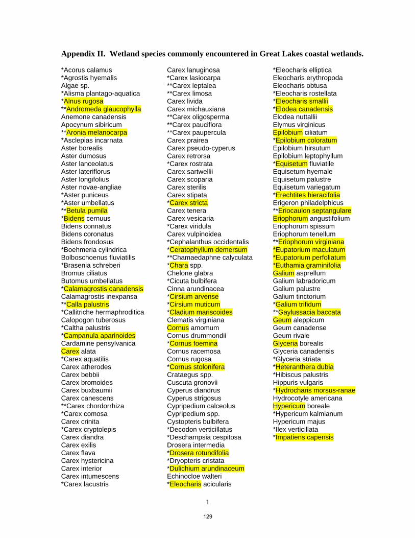
1

Appendix II. Wetland species commonly encountered in Great Lakes coastal wetlands. *Acorus calamus *Agrostis hyemalis Algae sp. *Alisma plantago-aquatica *Alnus rugosa **Andromeda glaucophylla Anemone canadensis Apocynum sibiricum **Aronia melanocarpa *Asclepias incarnata Aster borealis Aster dumosus Aster lanceolatus Aster lateriflorus Aster longifolius Aster novae-angliae *Aster puniceus *Aster umbellatus **Betula pumila *Bidens cernuus Bidens connatus Bidens coronatus Bidens frondosus *Boehmeria cylindrica Bolboschoenus fluviatilis *Brasenia schreberi Bromus ciliatus Butomus umbellatus *Calamagrostis canadensis Calamagrostis inexpansa **Calla palustris *Callitriche hermaphroditica Calopogon tuberosus *Caltha palustris *Campanula aparinoides Cardamine pensylvanica Carex alata *Carex aquatilis Carex atherodes Carex bebbii Carex bromoides Carex buxbaumii Carex canescens **Carex chordorrhiza *Carex comosa Carex crinita *Carex cryptolepis Carex diandra Carex exilis Carex flava Carex hystericina Carex interior Carex intumescens *Carex lacustris

Carex lanuginosa *Carex lasiocarpa **Carex leptalea **Carex limosa Carex livida Carex michauxiana **Carex oligosperma **Carex pauciflora **Carex paupercula Carex prairea Carex pseudo-cyperus Carex retrorsa *Carex rostrata Carex sartwellii Carex scoparia Carex sterilis Carex stipata *Carex stricta Carex tenera Carex vesicaria *Carex viridula Carex vulpinoidea *Cephalanthus occidentalis *Ceratophyllum demersum **Chamaedaphne calyculata *Chara spp. Chelone glabra *Cicuta bulbifera Cinna arundinacea *Cirsium arvense *Cirsium muticum *Cladium mariscoides Clematis virginiana Cornus amomum Cornus drummondii *Cornus foemina Cornus racemosa Cornus rugosa *Cornus stolonifera Crataegus spp. Cuscuta gronovii Cyperus diandrus Cyperus strigosus Cypripedium calceolus Cypripedium spp. Cystopteris bulbifera *Decodon verticillatus *Deschampsia cespitosa Drosera intermedia *Drosera rotundifolia *Dryopteris cristata *Dulichium arundinaceum Echinocloe walteri *Eleocharis acicularis

*Eleocharis elliptica Eleocharis erythropoda Eleocharis obtusa *Eleocharis rostellata *Eleocharis smallii *Elodea canadensis Elodea nuttallii Elymus virginicus Epilobium ciliatum *Epilobium coloratum Epilobium hirsutum Epilobium leptophyllum *Equisetum fluviatile Equisetum hyemale Equisetum palustre Equisetum variegatum *Erechtites hieracifolia Erigeron philadelphicus **Eriocaulon septangulare Eriophorum angustifolium Eriophorum spissum Eriophorum tenellum **Eriophorum virginiana *Eupatorium maculatum *Eupatorium perfoliatum *Euthamia graminifolia Galium asprellum Galium labradoricum Galium palustre Galium tinctorium *Galium trifidum **Gaylussacia baccata Geum aleppicum Geum canadense Geum rivale Glyceria borealis Glyceria canadensis *Glyceria striata *Heteranthera dubia *Hibiscus palustris Hippuris vulgaris *Hydrocharis morsus-ranae Hydrocotyle americana Hypericum boreale *Hypericum kalmianum Hypericum majus *Ilex verticillata *Impatiens capensis

129

2

Appendix II, continued *Iris versicolor *Iris virginica Juncus alpinus *Juncus balticus Juncus brevicaudatus Juncus bufonius Juncus canadensis Juncus dudleyi Juncus effusus Juncus greenei Juncus nodosus Juncus pelocarpus Juncus tenuis **Kalmia polifolia Lathyrus palustris **Ledum groenlandicum *Leersia oryzoides *Lemna minor *Lemna trisulca Liatris spicata Lobelia dortmanna *Lobelia kalmii Lobelia siphilitica Lobelia spicata Ludwegia palustris *Lycopus americanus *Lycopus uniflorus Lysimachia ciliata Lysimachia nummularia Lysimachia quadriflora Lysimachis terrestris *Lysimachis thyrsiflora Lythrum alatum *Lythrum salicaria Matteuccia struthiopteris *Megalodonta beckii *Mentha arvensis *Mentha piperita **Menyanthes trifoliata *Mimulus ringens Muhlenbergia glomerata Muhlenbergia unifloris Myosotis laxa Myosotis scorpioides Myosoton aquaticum *Myrica gale Myrica pensylvanica Myriophyllum alterniflorum *Myriophyllum exalbescens *Myriophyllum heterophyllum *Myriophyllum spicatum Myriophyllum tenellum Myriophyllum verticillatum

*Najas flexilis Najas minor *Nelumbo lutea *Nemopanthus mucronata *Nitella spp. *Nuphar advena *Nuphar variegata *Nymphaea odorata *Onoclea sensibilis Osmunda cinnamomea Osmunda regalis Panicum lindheimeri Panicum virgatum **Parnassia glauca *Peltandra virginica Penthorum sedoides *Phalaris arundinacea *Phragmites australis Physostegia virginiana Pilea fontana *Pilea pumila Platanthera clavellata Poa palustris Pogonia ophioglossoides *Polygonum amphibium *Polygonum hydropiperoides *Polygonum lapathifolium Polygonum pensylvanicum Polygonum persicaria Polygonum punctatum Polygonum sagittatum *Pontederia cordata Potamogeton alpinus Potamogeton amplilfolius Potamogeton berchtoldii *Potamogeton crispus Potamogeton epihydrus Potamogeton filiformis Potamogeton foliosus *Potamogeton friesii *Potamogeton gramineus *Potamogeton illinoensis *Potamogeton natans Potamogeton nodosus Potamogeton obtusifolius Potamogeton pectinatus Potamogeton perfoliatus Potamogeton praelongus Potamogeton pusillus *Potamogeton richardsonii Potamogeton robbinsii Potamogeton spirillus Potamogeton strictifolius

*Potamogeton zosteriformis *Potentilla anserina *Potentilla fruticosa *Potentilla palustris Prenanthes racemosa Proserpinaca palustris Pycnanthemum virginianum Ranunculus abortivus Ranunculus longirostris Ranunculus pensylvanicus Ranunculus recurvatus Ranunculus sceleratus *Rhamnus alnifolia *Rhamnus frangula *Rhynchospora alba *Rhynchospora capillacea *Rorippa palustris *Rosa palustris Rubus hispidus Rubus pubescens Rubus strigosus *Rumex crispus Rumex maritimus *Rumex orbiculatus *Sagittaria graminea *Sagittaria latifolia Sagittaria montevidensis *Sagittaria rigida Sagittaris cuneata Salix amygdaloides Salix bebbiana Salix candida Salix cordata Salix discolor Salix eriocephala *Salix exigua Salix lucida Salix myricoides Salix pedicellaris Salix petiolaris Salix pyrifloia Salix sericea Salix serissima *Sarracenia purpurea *Saururus cernuus *Scheuchzeria palustris *Schoenoplectus acutus *Schoenoplectus pungens *Schoenoplectus subterminalis *Schoenoplectus tabernaemontani Scirpus atrovirens Scirpus cespitosus Scirpus cyperinus

130

3

Appendix II, continued *Scutellaria galericulata Scutellaria lateriflora *Sium suave *Solanum dulcamara Solidago gigantean *Solidago ohioensis Solidago patula Solidago rugosa Solidago uliginosa Sparganium americanum *Sparganium chlorocarpum *Sparganium eurycarpum *Sparganium fluctuans *Sparganium minimum *Spartina pectinata *Sphagnum spp. *Spiraea alba Spiraea tomentosa Spiranthes cernua Spiranthes romanzoffiana *Spirodela polyrhiza Stachys palustris Stachys tenuifolia *Symplocarpus foetidus *Teucrium canadense Thalictrum dasycarpum *Thelypteris palustris *Tofieldia glutinosa *Triadenum fraseri Triadenum virginicum Triglochin maritimum *Triglochin palustre *Typha angustifolia *Typha latifolia *Typha x glauca *Urtica dioica *Utricularia cornuta *Utricularia intermedia Utricularia resupinatua *Utricularia vulgaris Vaccinium corymbosum *Vaccinium macrocarpon *Vaccinium oxycoccos *Vallisneria americana Verbena hastate Veronica anagalis-aquatica Veronica officinalis Viburnum lentago Viola cucullata Vitis riparia *Wolffia columbiana *Wolffia punctata Xyris montana *Zannichellia palustris Zanthoxylum americanum

*Zizania aquatic *Zizania aquatica var. aquatic

SUMMARY OF CODES

*= Common plant in most marshes (except Lake Superior for many) **= Common plant in Lake Superior marshes Genus highlighted = know how to recognize this genus

Genus and species highlighted = know this species

131

3/10/2011 

Wetland Bird Census Protocol  1. The wetland bird survey will be conducted twice at each point (2 resamples). 

a. Surveys will be conducted during the period of late May through early July (the breeding period). 

b. One resample will be a morning survey and one will be an evening survey. c. Resamples will occur no closer than 15 days apart. 

2. Survey weather a. Surveys should only be conducted during “good weather” (i.e. wind <15mph and 

little or no precipitation.  If the rain is falling harder than a light mist, you should probably discontinue the survey; however, there are times when bird activity picks up during a light rain.   

b. The decision to discontinue a survey due to wind is complicated by the fact that the wind often gusts, resulting in unacceptable conditions sometimes and acceptable conditions during other times.  The decision as to whether or not you should conduct or continue to conduct a survey is at times a largely subjective one.  

c.  Do not survey when weather conditions affect the birds’ singing.  The question underlying this decision is: Are there noticeably fewer birds singing as a result of the weather?  If so, you should discontinue the survey.   

d. In addition to the weather data, be sure to provide details on the data sheet if a survey is done during questionable weather. 

3. Sampling periods a. Morning surveys: sampling begins ½ hour before sunrise and ends 4 hours after 

sunrise. b. Evening surveys: sampling begins 4 hours before sunset and ends ½ hour after 

sunset. 4. Wetland sites & sample points 

a. A wetland site can contain from 1 to 12 sample points. b. Sample points  

i. Points are separated by a minimum of 250 meters. ii. If the point location is already loaded onto GPS unit, proceed to the 

provided point location. iii. If the point location needs to be determined, locate the point according 

to point selection protocol.  Be sure to save it into your GPS unit as a waypoint, using the appropriate point ID. 

c. Full‐circle sample points will be used, with distance intervals 0‐50 meters, 50‐100 meters and 100+ meters from the observer, as well as a line delineating the 180° semicircle areas in front of and behind the observer. 

a. Before beginning the survey, fill out the following:  i. Point ID: Each point has an associated ID.  ii. Resample: Each point will be visited 2 times for repeat surveys. iii. Date: Format of MM/DD/YY  (05/04/11). iv. Observer: Observer first initial and last name (D. Waters). v. Weather: Circle the appropriate description: dry, damp/haze/fog, drizzle or 

rain. vi. % Cloud Cover: Estimate the percentage of cloud cover in 10% increments. vii. Wind 

132

3/10/2011 

1. Beaufort wind scale codes (see chart below). 2. Only codes 0‐3 are acceptable conditions for conducting the survey. 

viii. Air Temperature  1. Take at chest height in the shade. 2. Record in °Celsius.  See the conversion chart on the Reference Sheet 

if needed. ix. Noise: Assign & record the appropriate noise code (see chart below). x. Bearing: Take the bearing while facing forward (toward the wetland).   

BEAUFORT WIND SCALE 0  Calm; smoke rises vertically 

1  Light air movement; smoke drifts; leaves barely move 

2  Slight breeze; wind felt on face; small twigs move 

3  Gentle breeze; leaves & small twigs in constant motion 

4  Moderate breeze; small branches moving, raises dust & loose paper 

5  Large branches & small trees sway 

 NOISE CODES 

0  No appreciable effect (owl calling) 

1  Slightly affecting sampling (distant traffic, dog barking, car passing) 

2  Moderately affecting sampling (distant traffic, 2‐5 cars passing) 

3  Seriously affecting sampling (continuous traffic nearby, 6‐10 cars passing) 

4  Profoundly affecting sampling (continuous traffic passing, construction noise) 

 c. Conduct the survey. 

i. Fill in the Start Time. 1. Record in 24‐hour format (8:43am is 0843; 2:56pm is 1456). 2. Time recorded as Eastern Daylight Time (observers in the central 

time zone, add 1 hour). ii. Start stopwatch or set timer. i. Each sample is broken down into 3 time periods: 

1. 0‐5 minutes: passive listening 2. 5‐10 minutes: playback 3. 10‐15 minutes: passive listening 

ii. Playback 1. Playback Order: the following playback compilation will be 

provided in one audio file (mp3 format). a. 30 seconds  VIRGINIA RAIL b. 30 seconds   silence c. 30 seconds   SORA d. 30 seconds   silence e. 30 seconds   LEAST BITTERN f. 30 seconds   silence g. 30 seconds   COMMON MOORHEN h. 30 seconds   silence i. 30 seconds   PIED‐BILLED GREBE j. 30 seconds   silence 

133

3/10/2011 

iii. Use the decibel meter before beginning the first survey each day to determine the speakers are projecting at 80db at 1m distance from the speaker.  Adjust volume if necessary. 

iv. Hold the speaker(s) above the level of vegetation and broadcast in the direction of the bearing you recorded. 

d. Record the data i. Each individual must be recorded, identified or not.  Individuals which 

cannot be positively identified should be recorded as unidentified (i.e. unidentified sparrow, unidentified woodpecker…see Reference Sheet for alpha codes).  The inability to identify every bird is expected.  What is not acceptable, however, is not recording individuals you are unable to identify—this can greatly affect survey results. 

ii. Record the 4‐letter alpha code for the species at the corresponding spatial location on the data sheet. 

iii. Record the behavior of the individual.  Notation examples are listed on each data sheet.  For instance, if it was singing, circle the alpha code; if it was calling, underline it.  “Observed” means you saw the bird and it wasn’t singing, calling or drumming. 

iv. Record the time period in which the bird was first detected by using a superscript after the alpha code.  The notation is listed on each data sheet.    1. For focal species, record ALL time periods the bird is detected in, 

using commas to separate the numbers in the superscript. 2. Focal species include: 

i. American Bittern ii. American Coot iii. Black Rail iv. Common Moorhen v. King Rail vi. Least Bittern vii. Pied‐billed Grebe viii. Sora ix. Virginia Rail x. Yellow Rail 

2. Example:  

PBGR2,5,10,14  

v. Record the breeding evidence code by using a subscript after the alpha code.  The most common breeding evidence codes can be found on the data sheet; more can be found, along with descriptions, on the Reference Sheet. 

vi. If the bird moves to a different location, record the movement with an arrow from the original location to the new location and record a point (.) at the new location.  This is for your own reference ONLY.  When entering the data, only the location where the bird was originally detected will be entered. 

134

3/10/2011 

vii. If a bird is detected at multiple stations, record it on all data sheets.  Record the detection normally on the data sheet for the station where the bird is closest; for all others, record it and make a note that it was detected at multiple points, closest on “X” data sheet (fill in the point ID).  

viii. Document all aerial foragers within the 100‐meter boundary of the station.  Record the species code in the Aerial Foragers box and provide a total for each species.  Time codes or breeding evidence codes are not required. 

   

135

draf

t

AVIAN MONITORING Field Data Sheet

2011 Point ID:

Resample:

Date:

Start Time: EDT

Observer:

Weather: Dry Damp/Haze/Fog Drizzle Rain

% Cloud Cover: Wind:

Air Temp: °C Water Temp: °C

Noise: Aerial Foragers (within 100m)

species #

Breeding Evidence Codes (subscript): NAWAON NAWACN NAWANB NAWADD NAWAFY occupied nest carrying nest nest building distraction feeding material display young

°

100m 50m

2/24/2011 Second entry: ________________________

First entry: ________________________

Comments:

Behavior: NAWA NAWA —NAWA NAWA NAWA NAWA DOWOD singing calling flyover observed 2 males simultaneous woodpecker singing drumming

Time Codes (superscript): 0-1 minutes0 1-2 minutes1 2-3 minutes2 … 14-15 minutes14

136

3/10/2011 

Amphibian Calling Survey Standard Operating Procedures 

 1. Samples: The calling survey for amphibians will be conducted 3 times (3 samples) per point on evenings 

with little or no wind and according to minimum nighttime temperatures.  Surveys should occur within a reasonably short period of time after the minimum nighttime temperature has been reached.  Samples are to be conducted no fewer than 15 days apart.  Mist or light rain conditions are acceptable for conducting surveys. a. 1st Sample: nighttime temperatures have reached 5 °C / 41°F. b. 2nd Sample: nighttime temperatures have reached 10 °C / 50 °F. c. 3rd Sample: nighttime temperatures have reached 17 °C / 63 °F. 

2. Sampling period a. Check local weather information for the official sunset time. b. Sampling begins ½ hour after sunset. c. Sampling ends 4 ½ hours after sunset. d. Example: if sunset is 9:40pm, surveys will begin at 10:10pm and continue to 2:10am.  This results 

in 4 hours of sampling time. 3. Wetland sites & sample points 

a. A wetland site can contain from 1 to 6 sample points. b. Sample points  

i. Points are separated by a minimum of 500 meters. ii. If the point location is already loaded onto GPS unit, proceed to the provided point location. iii. If the point location needs to be determined, locate the point according to point selection 

protocol.  Be sure to save it into your GPS unit as a waypoint using the appropriate point ID. c. Full‐circle sample points will be used, with distance intervals 0‐50 meters, 50‐100 meters and 100+ 

meters from the observer, as well as a line delineating the 180° semicircle areas in front of and behind the observer. 

4. Conducting the survey a. At each station, your arrival may cause a decrease in the number of amphibians calling.  Wait 

quietly for 1‐2 minutes before beginning the survey. b. While waiting to begin the survey, fill out the following:  

i. Point ID: Each point has an associated ID.  ii. Sample: Each point will be visited 3 times for repeat calling surveys. iii. Date 

1. Format of MM/DD/YY  (05/04/11). 2. Be sure to advance the date for surveys conducted after midnight. 

iv. Observer: Observer first initial and last name (D. Waters). v. Weather: Circle the appropriate description: dry, damp/haze/fog, drizzle or rain. vi. % Cloud Cover: Estimate the percentage of cloud cover in 10% increments. vii. Wind 

1. Beaufort wind scale codes (see chart below). 2. Only codes 0‐3 are acceptable conditions for conducting the survey. 

viii. Air Temperature  1. Take at chest height. 2. Record in °Celsius.  See the conversion chart if needed. 

ix. Noise: Assign & record the appropriate noise code (see chart below). x. Bearing: Take the bearing while facing forward (toward the wetland). 

   

137

3/10/2011 

BEAUFORT WIND SCALE 0  Calm; smoke rises vertically 

1  Light air movement; smoke drifts; leaves barely move 

2  Slight breeze; wind felt on face; small twigs move 

3  Gentle breeze; leaves & small twigs in constant motion 

4  Moderate breeze; small branches moving, raises dust & loose paper 

5  Large branches & small trees sway 

 NOISE CODES 

0  No appreciable effect (owl calling) 

1  Slightly affecting sampling (distant traffic, dog barking, car passing) 

2  Moderately affecting sampling (distant traffic, 2‐5 cars passing) 

3  Seriously affecting sampling (continuous traffic nearby, 6‐10 cars passing) 

4  Profoundly affecting sampling (continuous traffic passing, construction noise) 

 c. Conduct the survey for 3 minutes. 

i. Fill in the Start Time. 1. Record in 24‐hour format (8:43am is 0843; 2:56pm is 1456). 2. Circle CDT (Central Daylight Time) or EDT (Eastern Daylight Time) accordingly. 

ii. Start stopwatch or set timer. iii. Using the appropriate species codes, individuals, small groups and choruses are mapped 

spatially within the appropriate distance interval(s) on the 360° map.  NOTE: It is important to record observations within the lines (DO NOT WRITE ON ANY LINE) so it is clear in which distance interval the observation belongs, or whether it is in the “front” 180° semi‐circle or the “back” semi‐circle.  For full choruses in multiple distance intervals, record in each distance interval as appropriate. 

 Examples:    CHFR                CHFR               CHFR      2‐7      2‐7              CHFR      2‐4                         2‐3           INCORRECT     CORRECT      CORRECT                if group is within          if group is spread        one interval                   amongst two intervals   iv. For each species code recorded (e.g. CHFR), record the calling code underneath the species 

code (1, 2 or 3), then a hyphen, then the number of individuals (for codes 1 & 2 only) in all appropriate distance intervals (<50m, 50‐100m, >100m). 

1. There may be more than one individual of a species in the same spatial location.   2. For full choruses (code 3), it is impossible to estimate the number of individuals, so 

do not record anything except the calling code.    Examples:   

CHFR    SPPE    NLFR   2‐7                    3       1‐1 

138

3/10/2011 

 v. Water Temp 

1. After the survey, take water temperature 1 meter from margin at 2cm depth, where safe to do so.  Record in °Celsius.  See the Reference Sheet for a conversion chart from °F to °C. 

 AMPHIBIAN SPECIES CODES 

AMTO  American Toad 

BCFR  Northern (Blanchard’s) Cricket Frog 

BULL  Bullfrog 

CHFR  Chorus Frog (Western/Boreal) 

CGTR  Cope’s Gray Treefrog 

FOTO  Fowler’s Toad 

GRTR  Gray Treefrog 

GRFR  Green Frog 

MIFR  Mink Frog 

NLFR  Northern Leopard Frog 

PIFR  Pickerel Frog 

SPPE  Spring Peeper 

WOFR  Wood Frog 

  CALLING CODES 

1  Calls not simultaneous; individuals can be accurately counted 

2  Some calls simultaneous; individuals can be reliably estimated 

3  Full chorus, calls continuous & overlapping; not reliably estimated 

  

5. Safety, Materials & Equipment a. For reasons of safety at night, each amphibian survey team should consist of two people, 

consisting of one observer and another “ride‐along” person (does not need to be a qualified observer).  i.  This survey is a single observer protocol—the ride‐along is not to influence the survey in 

any way.   ii. If both people are qualified observers, it is fine to take turns; the same observer does not 

need to conduct the survey at all points. b. For reasons of driving safety and data quality, observers conducting amphibian surveys at night 

will not then conduct bird surveys the following morning.  When amphibian surveys need to be conducted during the bird breeding season, the evening bird surveys are to be conducted during that time.   i. NOTE: This will necessitate a team of two splitting up to perform the evening bird surveys, 

then meeting back up again to then perform the evening amphibian surveys.      

139

3/10/2011 

c. Each team will be equipped with the following: i. Data sheets ii. Clipboard iii. Waterproof, permanent pens/markers (Rite in the Rain pen, ultra fine tip Sharpie marker) iv. Stopwatch/timer v. Compass vi. Thermometer, in metal or plastic case vii. Standard Operating Procedures viii. Codes Reference Sheet ix. Atlas (road map book) x. Site/point map(s) xi. GPS unit, with points loaded  xii. Headlamp xiii. Pepper spray xiv. Extra batteries xv. Each crew will carry spare equipment & materials 

  

Notes for data entry system: 1. Point ID 2. Sample: drop down list (1‐3) 3. Date: can enter MM/DD and year is default? 4. Start time: 4 digits, no need for a “:”; drop down menu for CDT or EDT 5. Observer (First initial & full last name) 6. Weather: drop down list (see protocol or data sheet) 7. % Cloud Cover: 10% increments 8. Air Temp (Celsius) 9. Noise: drop down list (0‐4) 10. Wind: drop down list, Beaufort Scale (0‐4) 11. Water Temp (Celsius) 12. Bearing (0‐360) 13. Sample records (for each observation): 

a. Species code: drop down list (4‐letter code, code list in protocol) b. Calling code: drop down list (1‐3) c. # of individuals (calling codes 1 & 2 only; calling code 3 will not have a number) d. Distance interval: drop down list (0‐50, 50‐100, 100+) e. Location compared to observer (check box for “within front 180° semicircle”) 

140

AMPHIBIAN MONITORING Field Data Sheet

2011 Point ID:

Sample:

Date: / / 2011

Start Time:

Observer:

Weather: Dry Damp/Haze/Fog Drizzle Rain

% Cloud Cover: Wind:

Air Temp: °C Water Temp: °C

Noise:

°

100m 50m

Observations: CHFR x-y

Calling Code Description

1 Calls not simultaneous; individuals can be accurately counted

2 Some calls simultaneous; individuals can be reliably estimated

3 Full chorus, calls continuous & overlapping; not reliably estimated

3/10/2011 2nd data entry (signature): ________________________

1st data entry (signature): ________________________

x = calling code (1, 2 or 3) y = number of individuals (1, or # > 1 if small group of the same species at the same location); leave blank for calling code 3

Comments:

CDT EDT

141