ATP-EMTP investigation of a new fault location method for ... · ATP-EMTP investigation of a new...
6
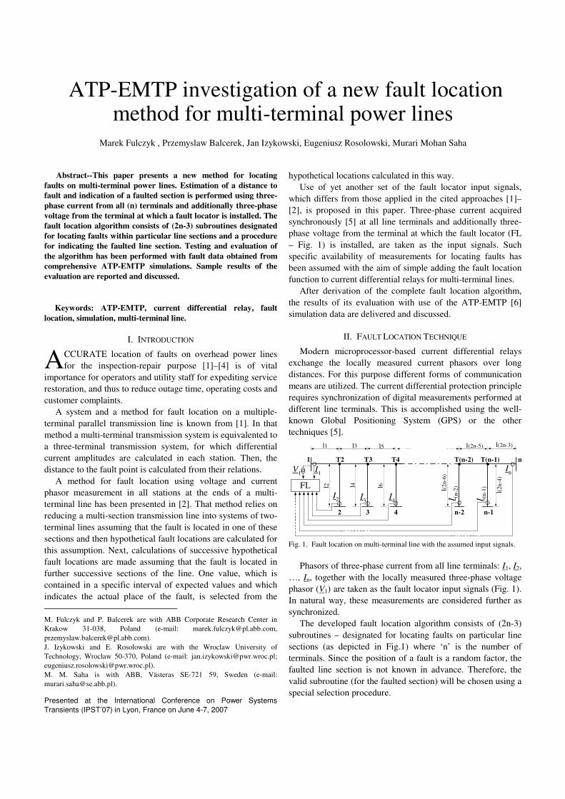
ATP-EMTP investigation of a new fault location method for multi-terminal power lines Marek Fulczyk , Przemyslaw Balcerek, Jan Izykowski, Eugeniusz Rosolowski, Murari Mohan Saha Abstract--This paper presents a new method for locating faults on multi-terminal power lines. Estimation of a distance to fault and indication of a faulted section is performed using three- phase current from all (n) terminals and additionally three-phase voltage from the terminal at which a fault locator is installed. The fault location algorithm consists of (2n-3) subroutines designated for locating faults within particular line sections and a procedure for indicating the faulted line section. Testing and evaluation of the algorithm has been performed with fault data obtained from comprehensive ATP-EMTP simulations. Sample results of the evaluation are reported and discussed. Keywords: ATP-EMTP, current differential relay, fault location, simulation, multi-terminal line. I. INTRODUCTION CCURATE location of faults on overhead power lines for the inspection-repair purpose [1]–[4] is of vital importance for operators and utility staff for expediting service restoration, and thus to reduce outage time, operating costs and customer complaints. A system and a method for fault location on a multiple- terminal parallel transmission line is known from [1]. In that method a multi-terminal transmission system is equivalented to a three-terminal transmission system, for which differential current amplitudes are calculated in each station. Then, the distance to the fault point is calculated from their relations. A method for fault location using voltage and current phasor measurement in all stations at the ends of a multi- terminal line has been presented in [2]. That method relies on reducing a multi-section transmission line into systems of two- terminal lines assuming that the fault is located in one of these sections and then hypothetical fault locations are calculated for this assumption. Next, calculations of successive hypothetical fault locations are made assuming that the fault is located in further successive sections of the line. One value, which is contained in a specific interval of expected values and which indicates the actual place of the fault, is selected from the M. Fulczyk and P. Balcerek are with ABB Corporate Research Center in Krakow 31-038, Poland (e-mail: [email protected], [email protected]). J. Izykowski and E. Rosolowski are with the Wroclaw University of Technology, Wroclaw 50-370, Poland (e-mail: [email protected]; [email protected]). M. M. Saha is with ABB, Västeras SE-721 59, Sweden (e-mail: [email protected]). Presented at the International Conference on Power Systems Transients (IPST’07) in Lyon, France on June 4-7, 2007 hypothetical locations calculated in this way. Use of yet another set of the fault locator input signals, which differs from those applied in the cited approaches [1]– [2], is proposed in this paper. Three-phase current acquired synchronously [5] at all line terminals and additionally three- phase voltage from the terminal at which the fault locator (FL – Fig. 1) is installed, are taken as the input signals. Such specific availability of measurements for locating faults has been assumed with the aim of simple adding the fault location function to current differential relays for multi-terminal lines. After derivation of the complete fault location algorithm, the results of its evaluation with use of the ATP-EMTP [6] simulation data are delivered and discussed. II. FAULT LOCATION TECHNIQUE Modern microprocessor-based current differential relays exchange the locally measured current phasors over long distances. For this purpose different forms of communication means are utilized. The current differential protection principle requires synchronization of digital measurements performed at different line terminals. This is accomplished using the well- known Global Positioning System (GPS) or the other techniques [5]. 1 2 3 4 n-2 n-1 n l(2n-6) l(2n-5) l(2n-4) l(2n-3) l1 l3 l4 l5 l6 T2 T3 T4 T(n-2) T(n-1) l2 FL I 1 I 2 I 3 I 4 I (n-2) I (n-1) I n V 1 Fig. 1. Fault location on multi-terminal line with the assumed input signals. Phasors of three-phase current from all line terminals: I 1 , I 2 , …, I n , together with the locally measured three-phase voltage phasor (V 1 ) are taken as the fault locator input signals (Fig. 1). In natural way, these measurements are considered further as synchronized. The developed fault location algorithm consists of (2n-3) subroutines – designated for locating faults on particular line sections (as depicted in Fig.1) where ‘n’ is the number of terminals. Since the position of a fault is a random factor, the faulted line section is not known in advance. Therefore, the valid subroutine (for the faulted section) will be chosen using a special selection procedure. A
Transcript of ATP-EMTP investigation of a new fault location method for ... · ATP-EMTP investigation of a new...
ATP-EMTP investigation of a new fault location method for multi-terminal power lines
Marek Fulczyk , Przemyslaw Balcerek, Jan Izykowski, Eugeniusz Rosolowski, Murari Mohan Saha
Abstract--This paper presents a new method for locating faults on multi-terminal power lines. Estimation of a distance to fault and indication of a faulted section is performed using three-phase current from all (n) terminals and additionally three-phase voltage from the terminal at which a fault locator is installed. The fault location algorithm consists of (2n-3) subroutines designated for locating faults within particular line sections and a procedure for indicating the faulted line section. Testing and evaluation of the algorithm has been performed with fault data obtained from comprehensive ATP-EMTP simulations. Sample results of the evaluation are reported and discussed.
Keywords: ATP-EMTP, current differential relay, fault
location, simulation, multi-terminal line.
I. INTRODUCTION
CCURATE location of faults on overhead power lines for the inspection-repair purpose [1]–[4] is of vital
importance for operators and utility staff for expediting service restoration, and thus to reduce outage time, operating costs and customer complaints.
A system and a method for fault location on a multiple-terminal parallel transmission line is known from [1]. In that method a multi-terminal transmission system is equivalented to a three-terminal transmission system, for which differential current amplitudes are calculated in each station. Then, the distance to the fault point is calculated from their relations.
A method for fault location using voltage and current phasor measurement in all stations at the ends of a multi-terminal line has been presented in [2]. That method relies on reducing a multi-section transmission line into systems of two-terminal lines assuming that the fault is located in one of these sections and then hypothetical fault locations are calculated for this assumption. Next, calculations of successive hypothetical fault locations are made assuming that the fault is located in further successive sections of the line. One value, which is contained in a specific interval of expected values and which indicates the actual place of the fault, is selected from the M. Fulczyk and P. Balcerek are with ABB Corporate Research Center in Krakow 31-038, Poland (e-mail: [email protected], [email protected]). J. Izykowski and E. Rosolowski are with the Wroclaw University of Technology, Wroclaw 50-370, Poland (e-mail: [email protected]; [email protected]). M. M. Saha is with ABB, Västeras SE-721 59, Sweden (e-mail: [email protected]). Presented at the International Conference on Power Systems Transients (IPST’07) in Lyon, France on June 4-7, 2007
hypothetical locations calculated in this way. Use of yet another set of the fault locator input signals,
which differs from those applied in the cited approaches [1]–[2], is proposed in this paper. Three-phase current acquired synchronously [5] at all line terminals and additionally three-phase voltage from the terminal at which the fault locator (FL – Fig. 1) is installed, are taken as the input signals. Such specific availability of measurements for locating faults has been assumed with the aim of simple adding the fault location function to current differential relays for multi-terminal lines.
After derivation of the complete fault location algorithm, the results of its evaluation with use of the ATP-EMTP [6] simulation data are delivered and discussed.
II. FAULT LOCATION TECHNIQUE
Modern microprocessor-based current differential relays exchange the locally measured current phasors over long distances. For this purpose different forms of communication means are utilized. The current differential protection principle requires synchronization of digital measurements performed at different line terminals. This is accomplished using the well-known Global Positioning System (GPS) or the other techniques [5].
1
2 3 4 n-2 n-1
n
l(2n-
6)l(2n-5)
l(2n-
4)
l(2n-3)l1 l3
l4
l5
l6
T2 T3 T4 T(n-2) T(n-1)
l2FL
I1
I2 I3 I4 I (n-2
)
I (n-1
)
InV1
Fig. 1. Fault location on multi-terminal line with the assumed input signals.
Phasors of three-phase current from all line terminals: I1, I2,
…, In, together with the locally measured three-phase voltage phasor (V1) are taken as the fault locator input signals (Fig. 1). In natural way, these measurements are considered further as synchronized.
The developed fault location algorithm consists of (2n-3) subroutines – designated for locating faults on particular line sections (as depicted in Fig.1) where ‘n’ is the number of terminals. Since the position of a fault is a random factor, the faulted line section is not known in advance. Therefore, the valid subroutine (for the faulted section) will be chosen using a special selection procedure.
A

A. Fault location algorithm – subroutine SUB_A
The subroutine SUB_A, designed for locating faults within the line section L1 (between nodes: 1, T2) (Fig. 2), is based on the following generalized fault loop model [4]:
0F1F1p1L111p =−− IRIZdV (1)
where
1d unknown distance to fault distance to fault from
the beginning of the line to the fault point (p.u.);
1FR unknown fault resistance;
1pV , 1pI fault loop voltage and current;
1L1Z positive sequence impedance of the section L1;
FI total fault current (fault path current).
Fault loop voltage and current are composed accordingly to the fault type, as the following weighted sums of the respective symmetrical components of the measured signals:
1001221111p VaVaVaV ++= (2)
101L1
0L10122111Ap I
ZZ
aIaIaI ++= (3)
where
1a , 2a , 0a weighting coefficients (Table I);
11V , 12V , 10V symmetrical components (the second lower
index) of voltages measured in station 1 (the first lower index);
A1I , A2I , A0I symmetrical components (the second lower
index) of currents measured in station 1 (the first lower index);
0L1Z , 1L1Z zero, positive sequence impedance
of the line section L1.
n
1d
2
iL11)(1 Zd−
2iLZ
11 iLZd
n-1
)n(iLZ 42 −
)n(iLZ 32 −1
1iI
T2 T(n-1)
Fig. 2. Equivalent circuit diagram of the network for the i-th symmetrical component assuming that a fault is on the first line section.
TABLE I WEIGHTING COEFFICIENTS IN FAULT LOOP SIGNALS (2)–(3)
FAULT TYPE 1a 2a 0a
a-g 1 1 1
b-g 35.0j5.0 −− 35.0j5.0 + 1
c-g 35.0j5.0 + 35.0j5.0 −− 1
a-b, a-b-g a-b-c, a-b-c-g 35.0j5.1 + 35.0j5.1 − 0
b-c, b-c-g 3j– 3j 0
c-a, c-a-g 35.0j5.1 +− 35.0j5.1 −− 0
Fault loop signals (2) and (3), and also those used in the remaining subroutines, are expressed in terms of the respective symmetrical components. Use of such notation is convenient for introducing the compensation for line shunt capacitances, however, it is fully equivalent to the description traditionally used for distance protection [4]. Natural sequence of phases: a, b, c was assumed for determining the weighting coefficients (Table I), as well as in all further symmetrical components calculations.
It is proposed to calculate the total fault current from (1) by using the following generalized fault model:
F0F0F2F2F1F1F IaIaIaI ++= (4)
where
F1a , F2a , F0a share coefficients (Table II).
TABLE II SHARE COEFFICIENTS USED IN FAULT MODEL (4)
FAULT TYPE F1a F2a F0a
a-g 0 3 0
b-g 0 3j1.51.5 + 0
c-g 0 3j1.5–1.5– 0
a-b 0 3j0.5–1.5 0
b-c 0 3j 0
c-a 0 35.0j5.1 −− 0
a-b-g 0 3j3 − 3j
b-c-g 0 32j 3j
c-a-g 0 3j3 −− 3j
a-b-c a-b-c-g
3j0.51.5 + 3j0.51.5 − *) 0
*) 0F2 ≠a , however, negative sequence component is not
present under three-phase balanced faults.
The i-th sequence component of the total fault current is determined as a sum of the i-th sequence components of currents from all line terminals (1, 2, …, n-1, n):
ni1)i-(n3i2i1iF1 ... IIIIII +++++= (5)
where subscript ‘i’ denotes the component type: i=1–positive, i=2–negative, i=0–zero sequence.
From the analysis of the boundary conditions of faults [4] results that it is possible to apply different alternative sets of the coefficients, which are used in (4). In order to assure high accuracy of fault location, use of the particular set has been recommended. The following priority for usage of particular sequence components (the respective coefficient in (4) is not equal to zero) of measured currents is proposed (Table II): - for phase-to-ground and phase-to-phase faults: use of negative sequence components; - for phase-to-phase-to-ground faults: use of negative and zero sequence components; - for three phase symmetrical faults: use of superimposed positive sequence components.
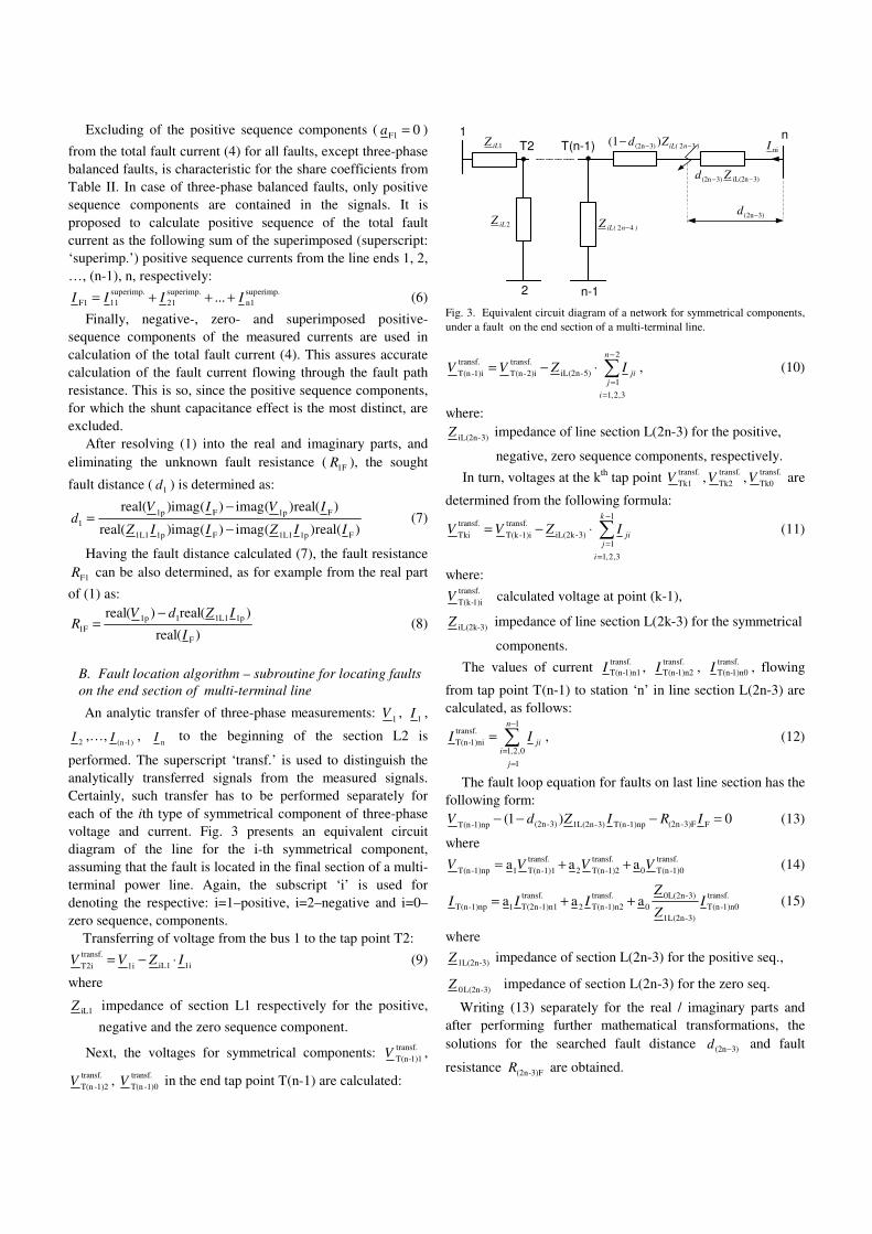
Excluding of the positive sequence components ( 0F1 =a )
from the total fault current (4) for all faults, except three-phase balanced faults, is characteristic for the share coefficients from Table II. In case of three-phase balanced faults, only positive sequence components are contained in the signals. It is proposed to calculate positive sequence of the total fault current as the following sum of the superimposed (superscript: ‘superimp.’) positive sequence currents from the line ends 1, 2, …, (n-1), n, respectively:
superimp.n1
superimp.21
superimp.11F1 ... IIII +++= (6)
Finally, negative-, zero- and superimposed positive-sequence components of the measured currents are used in calculation of the total fault current (4). This assures accurate calculation of the fault current flowing through the fault path resistance. This is so, since the positive sequence components, for which the shunt capacitance effect is the most distinct, are excluded.
After resolving (1) into the real and imaginary parts, and eliminating the unknown fault resistance ( 1FR ), the sought
fault distance ( 1d ) is determined as:
)(real)(imag)(imag)(real
)(real)(imag)(imag)(real
F1p1L1F1p1L1
F1pF1p1 IIZIIZ
IVIVd
−−
= (7)
Having the fault distance calculated (7), the fault resistance
F1R can be also determined, as for example from the real part
of (1) as:
)(real
)(real)(real
F
1p1L111p1F I
IZdVR
−= (8)
B. Fault location algorithm – subroutine for locating faults on the end section of multi-terminal line
An analytic transfer of three-phase measurements: 1V , 1I ,
2I ,…, 1)-(nI , nI to the beginning of the section L2 is
performed. The superscript ‘transf.’ is used to distinguish the analytically transferred signals from the measured signals. Certainly, such transfer has to be performed separately for each of the ith type of symmetrical component of three-phase voltage and current. Fig. 3 presents an equivalent circuit diagram of the line for the i-th symmetrical component, assuming that the fault is located in the final section of a multi-terminal power line. Again, the subscript ‘i’ is used for denoting the respective: i=1–positive, i=2–negative and i=0–zero sequence, components.
Transferring of voltage from the bus 1 to the tap point T2:
1iiL11itransf.T2i IZVV ⋅−= (9)
where
iL1Z impedance of section L1 respectively for the positive,
negative and the zero sequence component.
Next, the voltages for symmetrical components: transf.1)1-T(nV ,
transf.1)2-T(nV , transf.
1)0-T(nV in the end tap point T(n-1) are calculated:
2 n-1
niI
3)(2n−d)n(iLZ 42 −
3)iL(2n3)(2n −− Zd
)n(iLZd 323)(2n )(1 −−−
2iLZ
1iLZ T(n-1)T21 n
Fig. 3. Equivalent circuit diagram of a network for symmetrical components, under a fault on the end section of a multi-terminal line.
−
==
⋅−=2
3,2,11
5)-iL(2ntransf.
2)i-T(ntransf.
1)i-T(n
n
i
jjiIZVV , (10)
where:
3)-iL(2nZ impedance of line section L(2n-3) for the positive,
negative, zero sequence components, respectively.
In turn, voltages at the kth tap point transf.Tk1V , transf.
Tk2V , transf.Tk0V are
determined from the following formula:
−
==
⋅−=1
3,2,11
3)-iL(2ktransf.
1)i-T(ktransf.Tki
k
i
jjiIZVV (11)
where: transf.
1)i-T(kV calculated voltage at point (k-1),
-3)iL(2kZ impedance of line section L(2k-3) for the symmetrical
components.
The values of current transf.1)n1-T(nI , transf.
1)n2-T(nI , transf.1)n0-T(nI , flowing
from tap point T(n-1) to station ‘n’ in line section L(2n-3) are calculated, as follows:
−
==
=1
10,2,1
transf.1)ni-T(n
n
j
ijiII , (12)
The fault loop equation for faults on last line section has the following form:
0)1( F3)F-(2n1)np-T(n3)-L(2n13)-(2n1)np-T(n =−−− IRIZdV (13)
where transf.
1)0-T(n0transf.
1)2-T(n2transf.
1)1-T(n11)np-T(n aaa VVVV ++= (14)
transf.1)n0-T(n
3)-1L(2n
3)-0L(2n0
transf.1)n2-T(n2
transf.1)n1-T(2n11)np-T(n aaa I
Z
ZIII ++= (15)
where
3)-L(2n1Z impedance of section L(2n-3) for the positive seq.,
-3)L(2n0Z impedance of section L(2n-3) for the zero seq.
Writing (13) separately for the real / imaginary parts and after performing further mathematical transformations, the solutions for the searched fault distance 3)(2n−d and fault
resistance 3)F-(2nR are obtained.
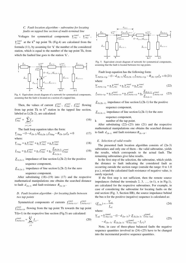
C. Fault location algorithm – subroutine for locating faults on tapped line section of multi-terminal line
Voltages for symmetrical components transf.Tk1V , transf.
Tk2V , transf.Tk0V at the kth tap point Tk (Fig.4) are calculated from the
formula (11), by assuming for ‘k’ the number of the considered station, which is equal to the number of the tap point Tk, from which the faulted line goes to the station ‘k’.
transf.TkiV transf.
1)iT(k+V
k k+1
transf.TkkiI
)k(iL)k( Zd 2222 −−
2)iL(2k2)(2k )(1 −−− Zd
)k(iLZ 2
)k(iLZ 2
2
1
2iLZ
1iLZ
n-1
)n(iLZ 42 −
)n(iLZ 32 − n
2)(2k−d
Fig. 4. Equivalent circuit diagram of a network for symmetrical components, assuming that the fault is located on a section of a tapped line.
Then, the values of current transf.Tkk1I , transf.
Tkk2I , transf.Tkk0I flowing
from tap point Tk to kth station in the tapped line section, labeled as L(2k-2), are calculated:
≠==
=n
kjj
ijiII
,13,2,1
transfTkki (16)
The fault loop equation takes the form: 0)1( F2)F-(2kTkkp2)-L(2k12)-(2kTkkp =−−− IRIZdV (17)
where: transf.Tkk00
transf.Tkk22
transf.Tkk11Tkkp aaa VVVV ++= (18)
transf.Tkk0
2)-1L(2k
2)-0L(2k0
transf.Tkk22
transf.Tkk11Tkkp aaa I
Z
ZIII ++= (19)
2)-L(2k1Z impedance of line section L(2k-2) for the positive
sequence component,
2)-L(2k0Z impedance of line section L(2k-2) for the zero
sequence component. After substituting (18)–(19) into (17) and the respective
mathematical manipulations one obtains the searched distance to fault 2)(2k−d and fault resistance 2)F-(2kR .
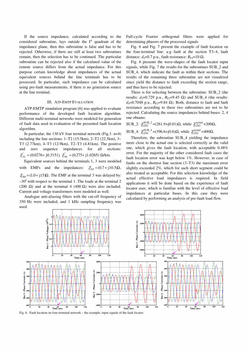
D. Fault location algorithm – for locating faults between two tap points
Symmetrical components of currents transf.1)1TkT(k+I , transf.
1)2TkT(k+I , transf.
1)0TkT(k+I flowing from the tap point Tk towards the tap point
T(k+1) in the respective line section (Fig.5) are calculated:
−
==
+ =1
10,2,1
transf.1)iTkT(k
k
j
ijiII , (20)
1
1)(2k−d
transf.TkiV transf.
1)iT(k+V
k k+1
transf.1)iTkT(k +I
)k(iLZ 22 −
1)iL(2kk)(2k )(1 −−− Zd
)k(iLZ 2
)k(iLZd 121)(2k −−
2
2iLZ
1iLZ
n-1
)n(iLZ 42 −
)n(iLZ 32 − n
Fig. 5. Equivalent circuit diagram of network for symmetrical components, assuming that the fault is located between two tap points.
Fault loop equation has the following form:
0)1( F1)F(2k1)pTkT(k1)L(2k11)(2k1)pTkT(k =−−− −+−−+ IRIZdV (21)
where transf.Tk00
transf.Tk22
transf.Tk111)pTkT(k aaa VVVV ++=+ (22)
transf.1)0TkT(k
1)1L(k
1)0L(k0
transf.1)2TkT(k2
transf.1)1TkT(k11)pTkT(k aaa +
+
++++ ++= I
Z
ZIII (23)
1)L(2k1 −Z impedance of line section L(2k-1) for the positive
sequence component,
1)L(2k0 −Z impedance of line section L(2k-1) for the zero
sequence component, k number of the tap point.
After substituting (22)–(23) into (21) and the respective mathematical manipulations one obtains the searched distance to fault 1)(2k−d and fault resistance 1)F(2k −R .
E. Selection of valid results The presented fault location algorithm consists of (2n-3)
subroutines and only one of them – the valid subroutine, yields the results, which corresponds to the actual fault. The remaining subroutines give false results.
In the first step of the selection, the subroutine, which yields the distance to fault indicating the considered fault as occurring outside the section range (outside the range: 0 to 1.0 p.u.), or/and the calculated fault resistance of negative value, is surely rejected.
If the first step is not sufficient, then the remote source impedances (behind the terminals 2, 3, …, (n-1), n in Fig.1), are calculated for the respective subroutines. For example, in case of considering the subroutine for locating faults on the end section (Fig. 3, Section IIB), the source impedance behind the bus n for the positive (negative) sequence is calculated as:
n2
n22Sn )(
I
VZ −= (24)
where:
)(
)1(
2transf.
1)n2-T(n3)-2L(2n3)(2n
transf.1)n2-T(n3)-2L(2n3)(2n
transf.1)2-T(nn2
FIIZd
IZdVV
−⋅⋅−
⋅⋅−−=
−
− (25)
Note, in case of three-phase balanced faults the negative sequence quantities involved in (24)–(25) have to be changed into the incremental positive sequence quantities.
If the source impedance, calculated according to the considered subroutine, lays outside the Ist quadrant of the impedance plane, then this subroutine is false and has to be rejected. Otherwise, if there are still at least two subroutines remain, then the selection has to be continued. The particular subroutine can be rejected also if the calculated value of the remote source differs from the actual impedance. For this purpose certain knowledge about impedances of the actual equivalent sources behind the line terminals has to be possessed. In particular, such impedance can be calculated using pre-fault measurements, if there is no generation source at the line terminal.
III. ATP-EMTP EVALUATION
ATP-EMTP simulation program [6] was applied to evaluate performance of the developed fault location algorithm. Different multi-terminal networks were modeled for generation of fault data used in evaluation of the presented fault location algorithm.
In particular, the 130 kV four terminal network (Fig.1: n=4) including the line sections: 1–T2 (15.5km), 2–T2 (22.5km), 3–T3 (2.77km), 4–T3 (12.9km), T2–T3 (4.81km). The positive and zero sequence impedances for all sections:
j0.3151)L += 0276.0(1'Z , j1.0265)L += 275.0(0
'Z Ω/km.
Equivalent sources behind the terminals 1, 3 were modeled
with EMFs and the impedances: Ω+= j10.5)7.0(S1Z ,
Ω+= j15)0.1(S0Z . The EMF at the terminal 3 was delayed by:
–30o with respect to the terminal 1. The loads at the terminal 2 (200 Ω) and at the terminal 4 (400 Ω) were also included. Current and voltage transformers were modeled as well.
Analogue anti-aliasing filters with the cut-off frequency of 350 Hz were included, and 1 kHz sampling frequency was used.
Full-cycle Fourier orthogonal filters were applied for determining phasors of the processed signals
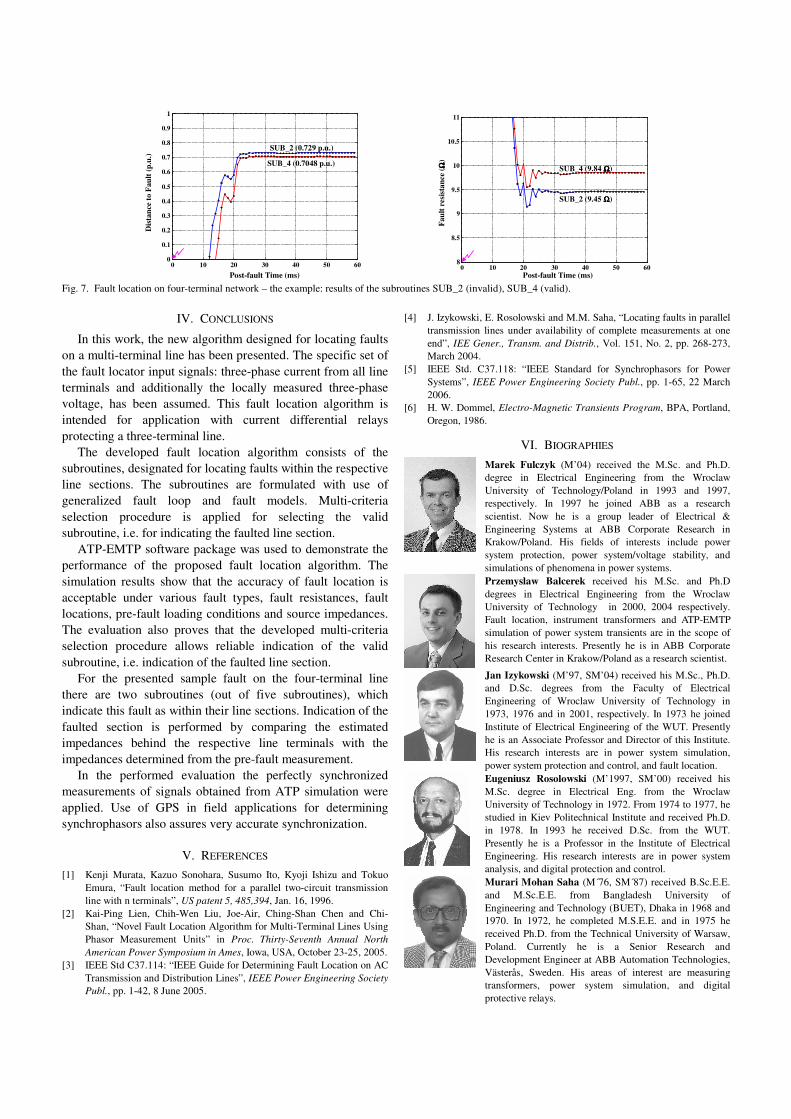
Fig. 6 and Fig. 7 present the example of fault location on the four-terminal line: a-g fault at the section T3–4, fault distance: d4=0.7 p.u., fault resistance: RF4=10 Ω.
Fig. 6 presents the wave-shapes of the fault locator input signals, while Fig. 7 the results for the subroutines SUB_2 and SUB_4, which indicate the fault as within their sections. The results of the remaining three subroutine are not visualized since yield the distance to fault exceeding the section range, and thus have to be rejected.
There is for selecting between the subroutine: SUB_2 (the results: d2=0.729 p.u., RF2=9.45 Ω) and SUB_4 (the results: d4=0.7048 p.u., RF2=9.84 Ω). Both, distance to fault and fault resistance according to these two subroutines are not to be rejected. Calculating the source impedances behind buses: 2, 4 one obtains:
SUB_2: SUB_22S2Z =(261.9+j0.01)Ω, while actual
2S2Z =200Ω,
SUB_4: SUB_42S4Z =(396.6+j0.6)Ω, while actual
2S2Z =400Ω.
Therefore, the subroutine SUB_4 yielding the impedance more close to the actual one is selected correctly as the valid one, which gives the fault location, with acceptable 0.48% error. For the majority of the other considered fault cases the fault location error was kept below 1%. However, in case of faults on the shortest line section (3–T3) the maximum error slightly exceeded 2%, which for such short segment could be also treated as acceptable. For this selection knowledge of the actual effective load impedances is required. In field applications it will be done based on the experience of fault locator user, which is familiar with the level of effective load impedances at particular buses. In this case they were calculated by performing an analysis of pre-fault load flow.
0 20 40 60 80 100 120
-1
-0.5
0
0.5
1
Bus
1 -
Phas
e V
olta
ges (
105 V
)
a b c
Time (ms) 0 20 40 60 80 100 120
-4000
-2000
0
2000
4000
Bus
1 -
Phas
e C
urre
nts (
A) a b c
Time (ms)
0 20 40 60 80 100 120-600
-400
-200
0
200
400
600
Bus
2 -
Phas
e C
urre
nts
(A)
a b c
Time (ms) 0 20 40 60 80 100 120
-4000
-2000
0
2000
4000
Bus
3 -
Pha
se C
urre
nts (
A)
Time (ms)
a b c
0 20 40 60 80 100 120
-300
-200
-100
0
100
200
300
Bus
4 -
Pha
se C
urre
nts (
A)
a b c
Time (ms) Fig. 6. Fault location on four-terminal network – the example: input signals of the fault locator.
0 10 20 30 40 50 600
0.1
0.2
0.3
0.4
0.5
0.6
0.7
0.8
0.9
1
Dis
tanc
e to
Fau
lt (p
.u.)
Post-fault Time (ms)
SUB_4 (0.7048 p.u.)
SUB_2 (0.729 p.u.)
0 10 20 30 40 50 60
8
8.5
9
9.5
10
10.5
11
Faul
t res
ista
nce
( ΩΩ ΩΩ)
Post-fault Time (ms)
SUB_4 (9.84 ΩΩΩΩ)
SUB_2 (9.45 ΩΩΩΩ)
Fig. 7. Fault location on four-terminal network – the example: results of the subroutines SUB_2 (invalid), SUB_4 (valid).
IV. CONCLUSIONS
In this work, the new algorithm designed for locating faults on a multi-terminal line has been presented. The specific set of the fault locator input signals: three-phase current from all line terminals and additionally the locally measured three-phase voltage, has been assumed. This fault location algorithm is intended for application with current differential relays protecting a three-terminal line.
The developed fault location algorithm consists of the subroutines, designated for locating faults within the respective line sections. The subroutines are formulated with use of generalized fault loop and fault models. Multi-criteria selection procedure is applied for selecting the valid subroutine, i.e. for indicating the faulted line section.
ATP-EMTP software package was used to demonstrate the performance of the proposed fault location algorithm. The simulation results show that the accuracy of fault location is acceptable under various fault types, fault resistances, fault locations, pre-fault loading conditions and source impedances. The evaluation also proves that the developed multi-criteria selection procedure allows reliable indication of the valid subroutine, i.e. indication of the faulted line section.
For the presented sample fault on the four-terminal line there are two subroutines (out of five subroutines), which indicate this fault as within their line sections. Indication of the faulted section is performed by comparing the estimated impedances behind the respective line terminals with the impedances determined from the pre-fault measurement.
In the performed evaluation the perfectly synchronized measurements of signals obtained from ATP simulation were applied. Use of GPS in field applications for determining synchrophasors also assures very accurate synchronization.
V. REFERENCES [1] Kenji Murata, Kazuo Sonohara, Susumo Ito, Kyoji Ishizu and Tokuo
Emura, “Fault location method for a parallel two-circuit transmission line with n terminals”, US patent 5, 485,394, Jan. 16, 1996.
[2] Kai-Ping Lien, Chih-Wen Liu, Joe-Air, Ching-Shan Chen and Chi-Shan, “Novel Fault Location Algorithm for Multi-Terminal Lines Using Phasor Measurement Units” in Proc. Thirty-Seventh Annual North American Power Symposium in Ames, Iowa, USA, October 23-25, 2005.
[3] IEEE Std C37.114: “IEEE Guide for Determining Fault Location on AC Transmission and Distribution Lines”, IEEE Power Engineering Society Publ., pp. 1-42, 8 June 2005.
[4] J. Izykowski, E. Rosolowski and M.M. Saha, “Locating faults in parallel transmission lines under availability of complete measurements at one end”, IEE Gener., Transm. and Distrib., Vol. 151, No. 2, pp. 268-273, March 2004.
[5] IEEE Std. C37.118: “IEEE Standard for Synchrophasors for Power Systems”, IEEE Power Engineering Society Publ., pp. 1-65, 22 March 2006.
[6] H. W. Dommel, Electro-Magnetic Transients Program, BPA, Portland, Oregon, 1986.
VI. BIOGRAPHIES
Marek Fulczyk (M’04) received the M.Sc. and Ph.D. degree in Electrical Engineering from the Wroclaw University of Technology/Poland in 1993 and 1997, respectively. In 1997 he joined ABB as a research scientist. Now he is a group leader of Electrical & Engineering Systems at ABB Corporate Research in Krakow/Poland. His fields of interests include power system protection, power system/voltage stability, and simulations of phenomena in power systems.
Przemyslaw Balcerek received his M.Sc. and Ph.D degrees in Electrical Engineering from the Wroclaw University of Technology in 2000, 2004 respectively. Fault location, instrument transformers and ATP-EMTP simulation of power system transients are in the scope of his research interests. Presently he is in ABB Corporate Research Center in Krakow/Poland as a research scientist.
Jan Izykowski (M’97, SM’04) received his M.Sc., Ph.D. and D.Sc. degrees from the Faculty of Electrical Engineering of Wroclaw University of Technology in 1973, 1976 and in 2001, respectively. In 1973 he joined Institute of Electrical Engineering of the WUT. Presently he is an Associate Professor and Director of this Institute. His research interests are in power system simulation, power system protection and control, and fault location.
Eugeniusz Rosolowski (M’1997, SM’00) received his M.Sc. degree in Electrical Eng. from the Wroclaw University of Technology in 1972. From 1974 to 1977, he studied in Kiev Politechnical Institute and received Ph.D. in 1978. In 1993 he received D.Sc. from the WUT. Presently he is a Professor in the Institute of Electrical Engineering. His research interests are in power system analysis, and digital protection and control.
Murari Mohan Saha (M´76, SM´87) received B.Sc.E.E. and M.Sc.E.E. from Bangladesh University of Engineering and Technology (BUET), Dhaka in 1968 and 1970. In 1972, he completed M.S.E.E. and in 1975 he received Ph.D. from the Technical University of Warsaw, Poland. Currently he is a Senior Research and Development Engineer at ABB Automation Technologies, Västerås, Sweden. His areas of interest are measuring transformers, power system simulation, and digital protective relays.


![3.1 การใช้โปรแกรม ATP-EMTP[2][5]dspace.spu.ac.th/bitstream/123456789/4684/5/5บทที่3.pdf · ของ BPA DCG/EPRI และ ATP-EMTP ของ](https://static.fdocuments.net/doc/165x107/5e862ef230e7a40dc403f3ef/31-aaaafaaaaaaaaa-atp-emtp25-aaaa3pdf.jpg)