Atomic Transport Phase Transformations - uni-stuttgart.de · Solid-Solid phase transformations...

Atomic Transport

&

Phase Transformations

Lecture 4

PD Dr. Nikolay Zotov

[email protected]

Lecture I-4 Outline

Classification of phase transitions

Solutions - Definitions

Types of solutions

Experimental determination of solubilities

Gibbs energy of solutions

Enthalpy of Mixing

Entropy of Mixing

Ideal Solid Solution Model

Substitutional Solutions - Hume-Rothery Rules

Interstitial Solutions - Rules

Phase Transitions (Transformations)

Examples:

Solid - Gas Sublimation

Solid - Liquid Melting

Liquid – Solid Solidification

Liquid - Gas Evaporation

Gas –Liquid Condensation

Definition:

Phase transition is a conversion (transformation) of one phase into another phase (at a constant composition).

Solid – Solid Polymorphic transition

Phase Transitions (Transformations)

Bismut

Phase Transitions

Classification

Classifications

Structural Thermodynamic

(solid-solid)

Other examples of Phase transitions:

# Conductor – to – insulator

# Normal – to - Superconductor

Phase TransitionsClassification

Solid – Solid phase transitions

Discontinuous Graphit → Diamant # Chemical bond breaking and reconstruction

(reconstructive) NaCl → CsCl-Typ # No Group-Subgroup relations between parent

hcp → fcc, fcc → hcp and product phase

Continuous

Displacive ß-Quarz → α-Quarz # Only small displacements of the atoms

Order-Disorder AuCu # Group – Subroup relations between parent and

product phase (Lecture 9)

7

Change of first coordination number (CN 4 ↔ 3)

No Group – Subgroup relation

P 63/mmc Fd3m

Phase TransitionsStructural Phase Transitions

Reconstructive

8

Space group Space groupP 31 21 P 62 2 2

Phase TransitionsStructural Phase Transitions

Displacive

The first coordinations of Si and Oxygen remains the same,only small rotations of the SiO4 tetrahedra

No change of translational symmetry (both lattices are primitive)Change only of the point-group symmetry ( 622 → 32)

Phase TransitionsThermodynamic Classifications (1)

Entropy Classification:

A) Discontinuous Phase Transitions

# The entropy is discontinuous DS;

# There is a latent heat L = Tc DS;

# Cp = - T(∂2G/∂T2) is finite for T ≠ TC

and undefined at TC.

B) Continuous Phase Transitions

# The entropy is continuous;

# No latent heat;

# Singularities in Cp and kT at TC.

Discontinuities

Divergences

G

G

T

T

TC

TC

TC TC

S

S

P. Ehrenfest

Phase TransitionsThermodynamic Classifications (2)

Ehrenfest Classification:

A) 1st Order Phase Transitions

# The first derivatives of the Gibbs free energy V= (∂G/∂p)T and S = - (∂G/∂T)p are

discontinuous (exhibit ‚jumps‘).

B) 2nd Order Phase Transitions

#The first derivatives of the Gibbs free energy (V and S) are continuous;

# The second derivatives Cp = - T(∂2G/∂T2)p and ßT = - (∂2G/∂p2)T/V

are discontinuous (exhibit ‚jumps‘) at the transition temperature

Phase TransitionsEhrenfest Classification

1. Order 2. Order

Latent heat L = TC(S1 – S2) No latent heat (L = 0)

(Heat is released/absorbed at T = const)

Co-existance of the two phase No coexistance of the two phase

Overheating/Undercooling possible Overheating/Undercooling not possible

Discontinuous phase transition Continuous phase transition

Solid-Solid phase transitons

No Group-Subgroup relations Group – Subgroup relations mandatory

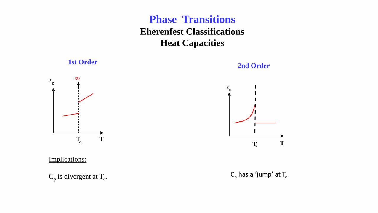
Phase TransitionsEherenfest Classifications

Heat Capacities

cp

T

cp

Tc

1st Order

T

cp

Tc

2nd Order

Implications:

Cp is divergent at Tc.Cp has a ‘jump’ at Tc

Phase TranisitonsExamples: H2O

Enthalpy Heat capacityJ/mol J/mol.K

6006 J/mol

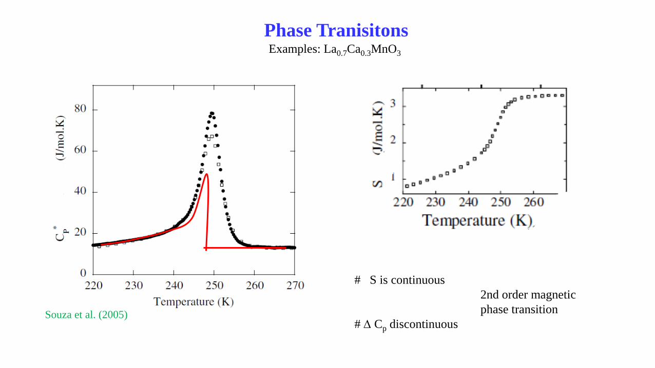
Phase TranisitonsExamples: La0.7Ca0.3MnO3

# S is continuous

2nd order magnetic

phase transition

# D Cp discontinuousSouza et al. (2005)


1. Order 2. Order

Coexsistance of the two phase No coexistance of the two phase

● Existence of Interface bewteen the

two phases – Growth of the product

phase through movement of

interfaces.

● Nucleation of the product phase in

the parent phase (Part III)

‚Spontaneous‘ change of structural state

in the whole macroscopic volume

Formation of domains

# change only of the point-group symmetry

Number of domains = PHT/PLT


PbTiO3 pervoskite

SG PG Order

HT P m -3 m m -3 m 48

LT P 4mm 4mm 8

Number of domains 48/8 = 6

Sicron et al. (1995)


Examples

1. Order 2. Order

Crystallization/Melting Feroelectricity

Sublimation Ferromagnetism

Condensation Normal-to-Superconducting state

Solid-Solid phase transformations Solid-solid phase transformation

Ce

Solutions

Definitions:

Solubility: The ability of a given component to dissolve into another component.

Solvent: The component in greater amount, which dissolves the minor component.

Solute: The component in lesser amount, which is dissolved.

Solubility Limit: The maximum amount (concentration) of the solute, which can be dissolved in the solvent.

Mechanical mixture: System consisting of two completely immissible components.

A solution is a homogeneous system ↔ it represents a single phase.

System with C = 2 and P = 1

Solutions

Alcohol Solubility in water at RT

[g Alc/100 mL water]

Methanol ∞

Ethanol ∞

Butanol 8.0

Hexanol 0.7

Solubility of sugar in water

Solubility changes with T and pressure !!!

Solutions

Types of solutions:

Gaseous

Liquid

Solid (Alloys)

Substitutional

Interstitial

Types of solutions:

Binary (C = 2)

Ternary (C = 3)

Multicomponent ( C > 3)B

A

C

SolutionsDetermination of Solubilities

Experimental methods:

# Solubility of metals in metals Diffusion experiments (Part II)

Quenching of liquid specimens

# Composition – Chemical methods, ICP, EDX SEM

# Homogeneity – Optical microscopy, Diffraction

Variation of the Crystallization/Melting temperature

of the solution with composition

DSC, DTA ( at ambient pressure)

SolutionsDetermination of Solubilities

In DSC/DTA the Cp peak broadens due to instrumental factors

(heating rate; mass of the sample, shape of sample, time lag, etc.)

The melting/crystallization temperaturs in DTA/DSC are

determined by the corresponding Onset Temperatures.

Melting is 1st Order Phase transtion → The Entalpy shows a jump.

Heat capacity Cp ~ dH/dT = Ŝ/ß ideally divergies at Tm.

Solutions

Determination of Solubilities

Schematic change of DTA/DSC peak

with alloying

Pure Ag (Tm = 961.8 oC)

DTA curves at three different heating rates (5, 10, 20 K/min)

Shift of onset temperatures, peak maximum with heating rate →

low heating/cooling rates for accurate results

Boettinger et al.

Elsevier, 2007

Boettinger et al.

Elsevier, 2007

Liquidus

SolutionsGibbs Energy

Mechanical mixture (C = 2):

G = nAGA + nBGB; N = nA + nB ( number of moles);

Molar Gibbs energy: Gm = XA GA + XB GB; XA + XB = 1

Implications:

Gm = (1 – XB) GA + XB GB;

The molar Gibbs energy of a mechanical

mixture is a linear sum of the Gibbs energies

XA = nA/(nA + nB); XB = nB/ (nA + nB);

Solution (C = 2):

Gsol = nAGA + nBGB + DGmix; DGmix - Gibbs energy of mixing

Solutions

Gibbs Energy

Implications:

Condition for the formation of a solution (1): DGmix < 0; but G = H – TS

Condition for the formation of a solution (2): DHmix < TDSmix

DHmix - Enthalpy of Mixing (Heat of formation of the solution);

DSmix - Entropy of Mixing (Entropy of formation of the solution).

Solutions

Enthalpy of Mixing

Water - Metanol Water - EthanolWater - Propanol

DH mix m = Q = Cp DT

Peteers et al. (1993)

Solutions

Enthalpy of Mixing

DH mix = Hsol – HA – HB;

H = U + pV ~ U

Solid (Liquid) Solutions

Neglect the kinetic energy of the species; U ~ Potential energy of the species

U = ½ S E2(rij) + E3(r) + ∙∙ ; E2 – pair-wise potential energy between species

E3 – tree-body potential energy

U = ½ S E2(rij) + Emany-body

Van-der-Waals crystals/liquids (noble gases at low T):

non-directional interactions

Lenard-Jones potential E2LJ = 4e[(s/r)12 - (s/r)6];

SolutionsEnthalpy of Mixing

Potentials

Ionic crystals/melts

non-directional, electrostatic interactions

E2ionic ~ C/r12 – e2/(4peor);

eo – dielectric constant of the vacuum


Potentials

Metals/metallic melts

non-directional, delocalized electron-electron

+ electron-core interactions


Potentials

Metals

Finnis-Sinclair (FS) potential

E2FS = (r - c)2(co + c1r + c2r

2); r ≤ c (cut-off)

Emany-bodyFS = - Si f(ri); r – Electron density of atom i;

f(r) = r ½ ; ri = S j≠i A2 f(rij); f(rij) = (rij-d)2; r ≤ d

A = 0.93 eV/Å

c = 2.96 Å

d = 4.05 Å

Cu a

c

Dai et al. (2006)

Covalent crystals/melts

strongly-directional interactions

Stillinger-Weber (SW) potential


Potentials

Covalent crystals

SW potential

E2SW = [B(s/r)4 – 1]exp(s/(r-as))

E3SW = exp(s/(rij – as))exp(s/(rik-as))(cos(Qjik + 1/3)2;

Sisp3 hybridisation

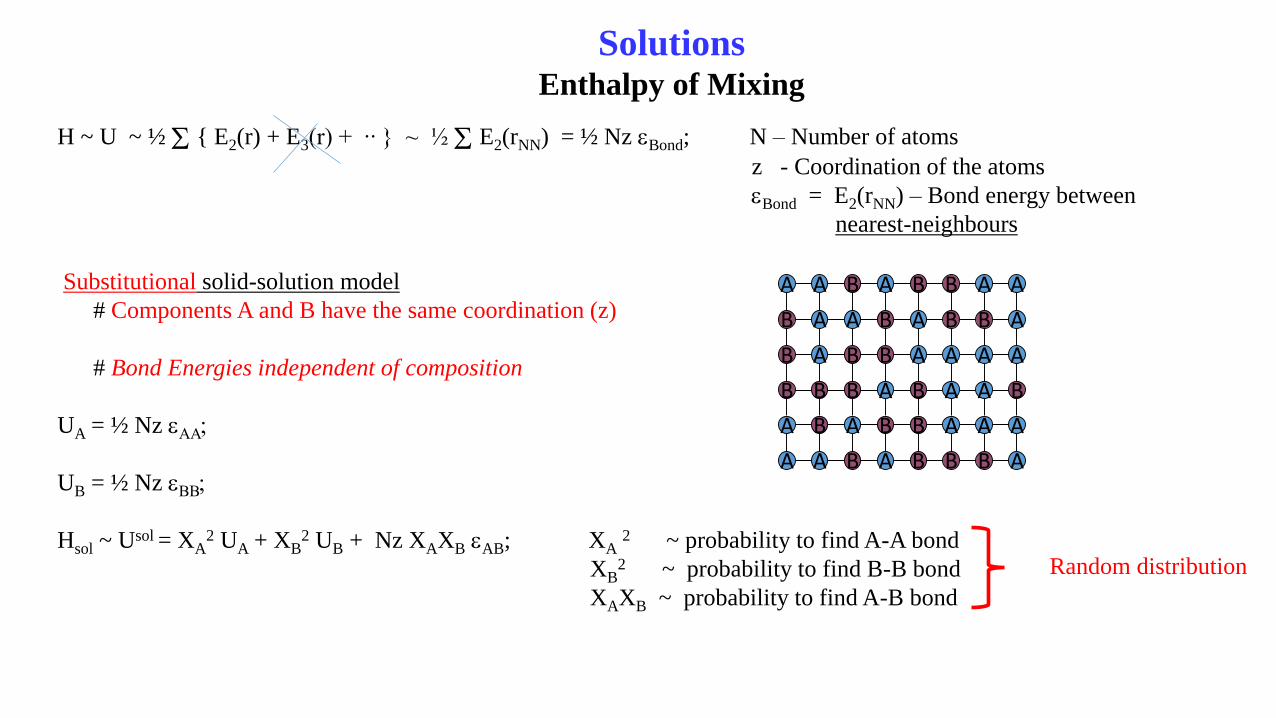
H ~ U ~ ½ S { E2(r) + E3(r) + ∙∙ } ~ ½ S E2(rNN) = ½ Nz eBond; N – Number of atoms

z - Coordination of the atoms

eBond = E2(rNN) – Bond energy between

nearest-neighbours

Substitutional solid-solution model

# Components A and B have the same coordination (z)

# Bond Energies independent of composition

UA = ½ Nz eAA;

UB = ½ Nz eBB;

Hsol ~ Usol = XA2 UA + XB

2 UB + Nz XAXB eAB; XA2 ~ probability to find A-A bond

XB2 ~ probability to find B-B bond

XAXB ~ probability to find A-B bond


A A

B A

AB

BA

B B

A B

AA

AB

B A

B B

BB

AB

A A

B A

AA

BA

A B

A A

BA

AB

B A

B B

AA

AB

Random distribution


DHmixm = XA

2 UA + XB2 UB + Nz XAXB eAB - XAUA - XBUB=

= ½ Nz eAA XA(1-XB) + ½ Nz eBB XB(1-XA) + Nz XAXB eAB - ½ Nz XAeAA - ½ Nz XBeBB =

= ½ Nz XAXB (2eAB – eAA – eBB) = ½ Nz XAXB De ; De = 2eAB – eAA – eBB .

= WXAXB ; W = ½ NzDe (N = NA)

Implications:

De > 0 DHmix > 0

De < 0 DHmix < 0

Ideal Solution Model: Solution for which the Enthalpy of mixing is zero (DHmix = 0).

DGmix = -TDSmix ;

Implications:

De = 0 → eAB = ½ (eAA + eBB); uniformity of the nearest-neighbhour interactions

eAB = eAA = eBB ; (not necessary condition)!!

DV mix = (∂DG mix/∂p)|T = 0 Vmid = XAVA

o+ XB VBo ;

SolutionsIdeal Solid Solution Model

SolutionsEntropy of Mixing

DS mix = Ssol – nASA – nBSB;

DS mix = kB ln(W)

W = Wvib Welec WConf ; DS mix = DS vib + DS Conf + DS Elec;

Vibrational Entropy:

For a single component system (C = 1) without electronic degrees of freedom and defects, the entropy arrises

from the vibrational degrees of freedom (Lecture 2)

S (vib) = - (∂G/∂T)p ;

Ssol = nASA + nBSB - (∂DGmix/∂p)T(∂p/∂T) = nASA + nBSB - DVmix(∂p/∂T)

DS mix (vib) = -(∂p/∂T) DVmix ; For the ideal solid-solution model DVmix = 0 → DS mixid(vib) ~ 0

# Substitutional solid solutions;

# DS mixid (vib) ~ 0;

# Neglecting electronic contributions to the entropy;

# Only contribution from the different possible arrangements of the A and B atoms in the lattice

considered (configurational entropy)

# ideal solid-solution model: similar forces between different types of atoms → random distribution is

the most probable:

W ~ Wconf = N!/ (XAN)! (XBN)! ; DS mix = kB ln[N!/ (XAN)! (XBN)! ]



DS mix = kB ln[N!/ (XAN)! (XBN)! ] = Sterling formula

= ···

= - kBN { XAlnXA + XBlnXB}; [= - kBN S Xiln(Xi) ] ; i = 1,2, ∙∙∙ C

N = NA; ( 1 mole solution)

Molar Entropy of mixing of the ideal solid solution model:

DS mixid = - R{XAlnXA + XBlnXB}

DS mix = XA SA + XB SB → Si = - R ln(Xi); partial molar entropies of the components


Max

XA = XB = 0.5

DS id mix m = Rln2 = 5.76 J/mol.K

DS mix id > 0

Increase of Entropy by

Mixing!!!

SolutionsGibbs energy of the ideal solution model

Gsol = nAGA + nBGB + DGmix;

Molar Gibbs energy

Gsol m = XAGA + XBGB + (DHmix m – TDSmix m)

Molar Gibbs energy of the ideal solution model:

G mid = XAGA + XBGB + TR {XAlnXA + XBlnXB}

DGmix = TR {XAlnXA + XBlnXB} < 0

The Gibbs energy of the ideal solution model decreases, compared to the

mechanical mixture XAGA + XBGB.

G mid has a minimum at XB = 1/{1 + exp[ (GB-GA)/2RT]}; if GA = GB ; min at XB= 0.5

T2 > T1

SolutionsGibbs energy of ideal solution model

Molar Gibbs energy of the ideal solution model:

1st Derivative: ∂DGidm/∂XB = RTln (XB/1-XB)

XB → 0 ∂DGidm/∂XB → ∞ Logarithmic divergence

# Addition of small amount of solute (vacancies) decreases the Gibbs energy due to the

configurational entropy

2nd Derivative: ∂2DGidm/∂XB

2 = RT(1/XB – 1/(1-XB) =

= RT/XB(1-XB)

Curvature k = ∂2DGidm/∂XB

2 / [(1 + (∂DGidm/∂XB )2]3/2 = RT/ {[XB(1 – XB)]{1 + [RTln (XB/1-XB)]2}3/2 }

maximum curvature kmax = 4RT at XB = ½

SolutionsIdeal Solid Solution - Summary

DeHoff (2006)

DSmixmax = 5.76 J/mol.K

SolutionsSubstitutional Solid Solutions

Questions: when are formed ideal substitutional solid solutions,

Hume-Rothery Rules:

1. 100 * | (Rsolute – Rsolvent)/RSolvent | < 15 %; R – atomic radius

2. Crystal structures very similar (identical);

3. Solute and Solvent atoms typically have the same valence;

4. Small difference in the electronegativities : | cA – cB | → 0.

W. Hume-Rothery

Hume – Rothery Rules

Examples:

Proprerty Al Cu

Radius (Å) 1.43 1.28 10%

Structure fcc fcc

Electonegativity 1.6 1.9

Valence state +3 +2(+1)

Limited solubility



Examples:

Proprerty Ni Cu

Radius (Å) 1.35 1.28 5%

Structure fcc fcc


Valence state +2 +2(+1) +2

Complete Solubility!!




Examples:

Proprerty Ag Cu

Radius (Å) 1.44 1.28 11%

Structure fcc fcc


Valence state +2(+1) +2(+1)

Limited solubility

(M) – Solid solution with M as solvent


Darken – Gurry Maps:

[ (c – cA)/0.2]2 + [ (r – rA)/0.075] 2 = 1

R. Ferro, Intermetallic Chemistry, Elsevier 2008


Darken – Gurry Maps:

SolutionsInterstitial Solid Solutions

Size of the Voids

RV ~ 0.7 Ratom;

Criteria for formation of interstitial solid solutions

# Number of Voids, coordination of interstitial atoms

# Degree of distortion of the host (solvent) lattice

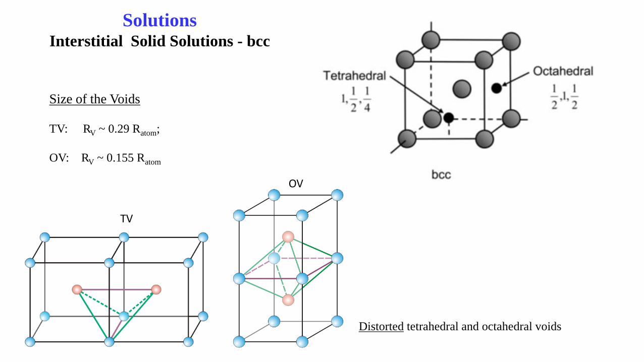
SolutionsInterstitial Solid Solutions - bcc

TV

OV

Distorted tetrahedral and octahedral voids

Size of the Voids

TV: RV ~ 0.29 Ratom;

OV: RV ~ 0.155 Ratom

SolutionsInterstitial Solid Solutions - fcc

TV OV

Size of the Voids



undistorted

SolutionsInterstial Solid Solutions - hcp

Size of the Voids (for ideal c/a ratio)



SolutionsInterstitial Solid Solutions

Type lattice Type of VoidCubic Tetrahedral Octahedral

SC 1 - -

bcc - 12 6

Fcc - 8 4

hcp - 4 2

SolutionsIntersititial Solid Solutions

RFe ~ 1.26 Å

Size of Voids (Å)

Lattice TV OV

bcc 0.37 0.20

Fcc 0.28 0.52

RC= 0.77 Å; RN = 0.71 Å; RH = 0.46Å

Bond Distortion

eB = (RI – RV) / RA = RI / RA - c;

Total Distortion ~ ½ NV zV eB x 100 (%)

Total DistortionLattice TV OV

bcc 7.7 % 8.1%

Fcc 6.2% 2.4%

Smaller distrotion - Larger Solubility

Atomic Transport Phase Transformations - uni-stuttgart.de · Solid-Solid phase transformations...

Documents

Transcript of Atomic Transport Phase Transformations - uni-stuttgart.de · Solid-Solid phase transformations...