ATOC 5051 INTRODUCTION TO PHYSICAL OCEANOGRAPHY Lecture...
24
ATOC 5051 INTRODUCTION TO PHYSICAL OCEANOGRAPHY Lecture 25: ENSO mechanisms Learning objective: Should know the major existing ENSO theories, and UNDERSTAND the ocean-atmosphere coupled processes for the “delayed-oscillator theory”. (1)The delayed-oscillator theory; (2) The recharge-discharge theory; (3)Stochastic forcing.
Transcript of ATOC 5051 INTRODUCTION TO PHYSICAL OCEANOGRAPHY Lecture...
ATOC 5051 INTRODUCTION TO PHYSICAL OCEANOGRAPHY Lecture 25: ENSO mechanisms
Learning objective: Should know the major existing ENSO theories, and UNDERSTAND
the ocean-atmosphere coupled processes for the “delayed-oscillator theory”.
(1)The delayed-oscillator theory; (2) The recharge-discharge theory; (3)Stochastic forcing.
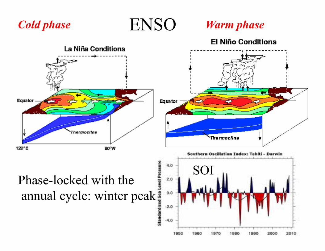
ENSO Cold phase Warm phase
SOI Phase-locked with the annual cycle: winter peak

1. ENSO Climatic Impacts: El Nino (warm phase) Impact: general pattern Can be different between strong & weak events
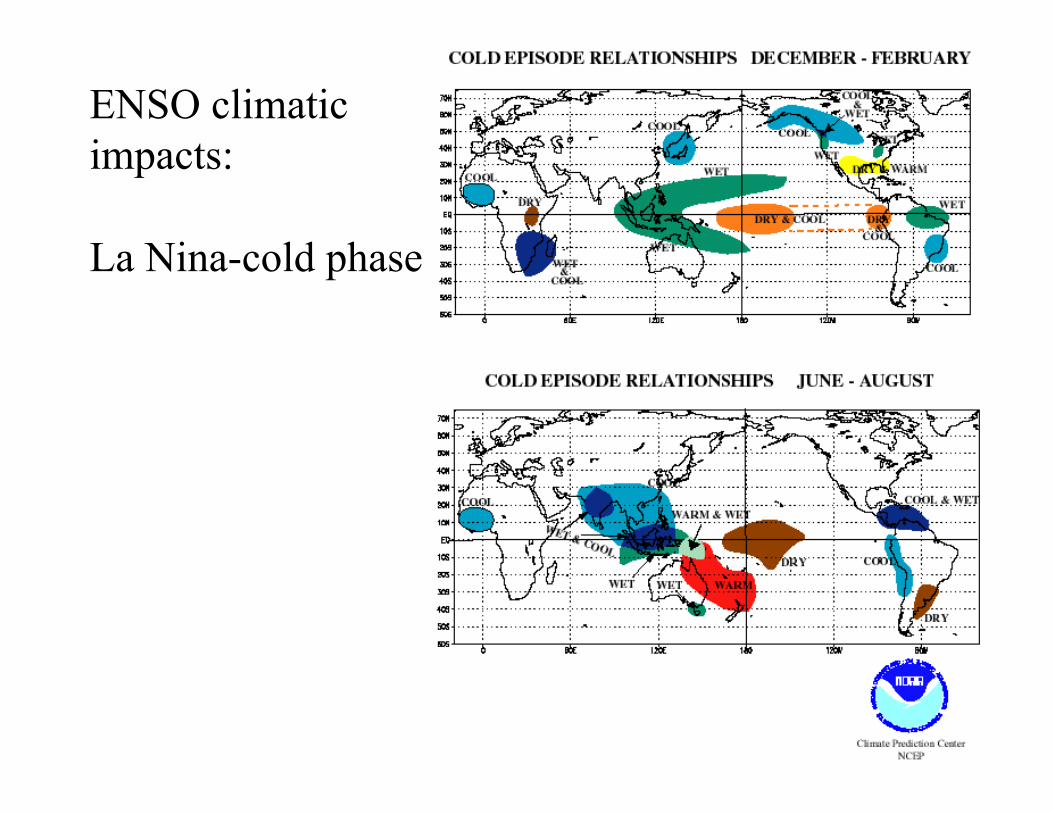
ENSO climatic impacts: La Nina-cold phase
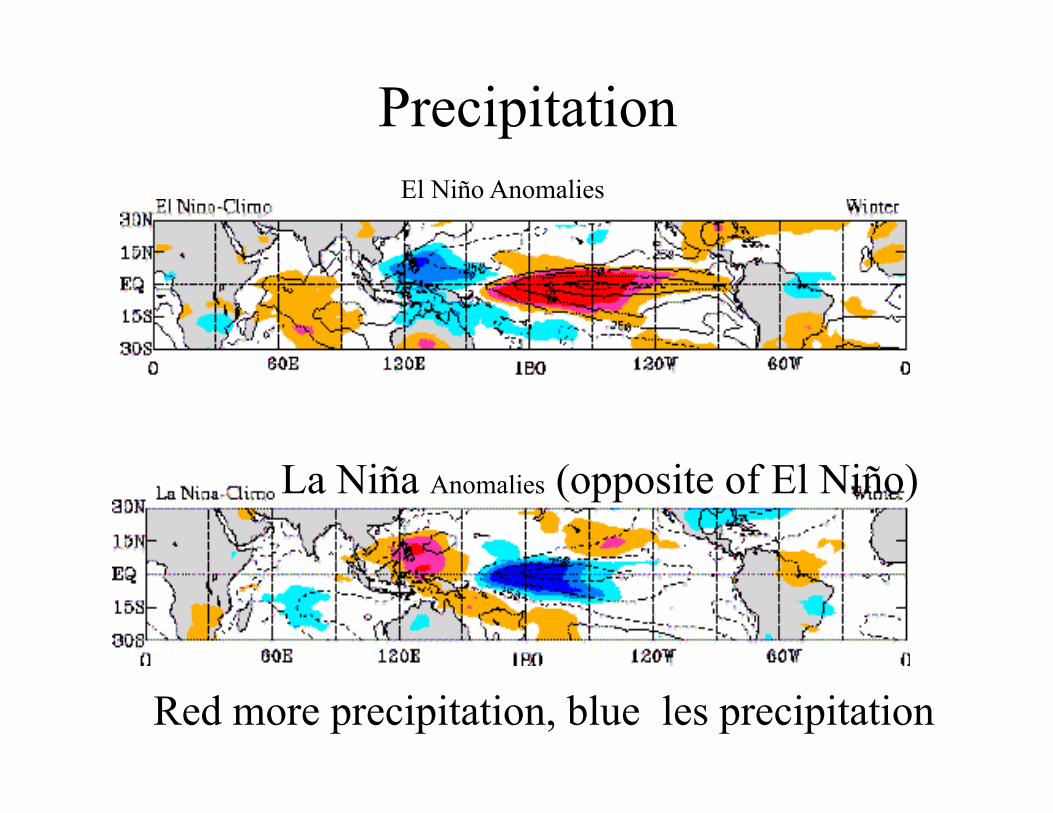
Precipitation El Niño Anomalies
La Niña Anomalies (opposite of El Niño)
Red more precipitation, blue les precipitation

Indian summer Monsoon drought associated El Nino: central pacific warming (rather than warming in the east)!!
Composite SST difference pattern between severe drought (shaded) and drought-free El Nino years. Composite SST anomaly patterns of drought-free years are shown as contours. From Kumar et al. 2006.
El Nino Modoki
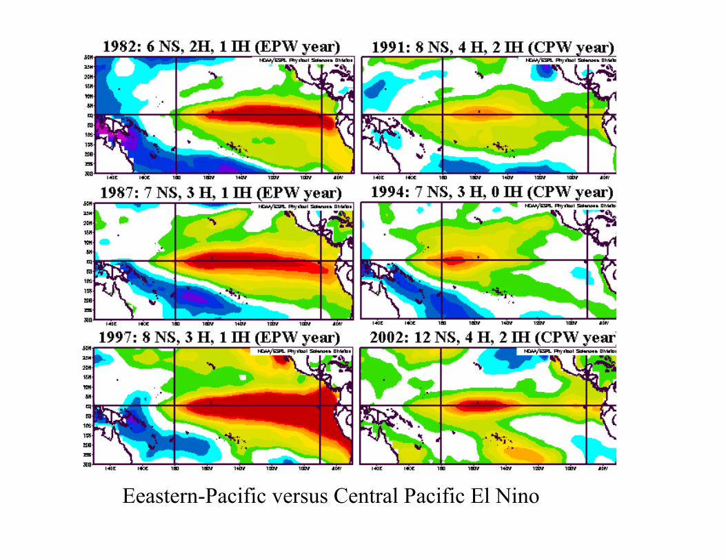
Eeastern-Pacific versus Central Pacific El Nino

Devastating Effects of El Nino
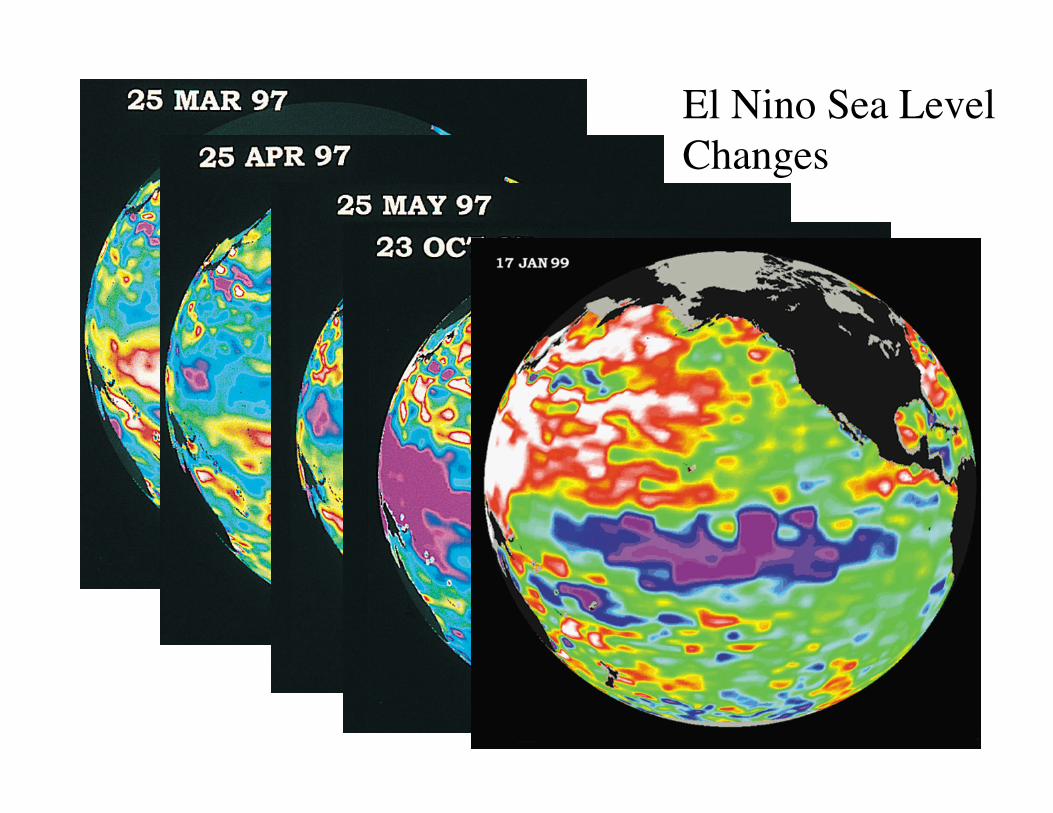
El Nino Sea LevelChanges
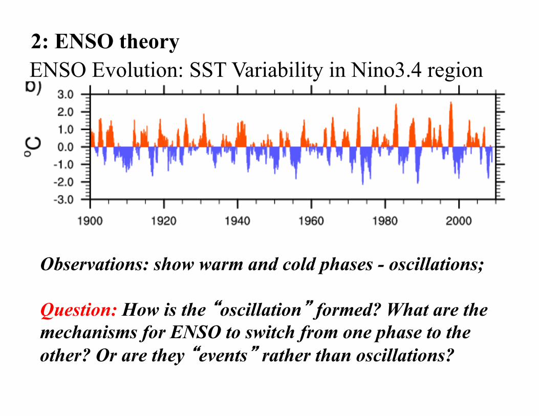
ENSO Evolution: SST Variability in Nino3.4 region 2: ENSO theory
Observations: show warm and cold phases - oscillations; Question: How is the “oscillation” formed? What are the mechanisms for ENSO to switch from one phase to the other? Or are they “events” rather than oscillations?

ENSO theory
(1) Delayed oscillator theory; (2) Charge-recharge theory; (3) Stochastic forcing.

(1) The delayed-oscillator theory (Clarke 2008)
Recall the mean SST pattern:
Warm Pool
Cold tongue
Large SST gradient
28.5C line: Near 180E

The delayed-oscillator theory (Clarke 2008)
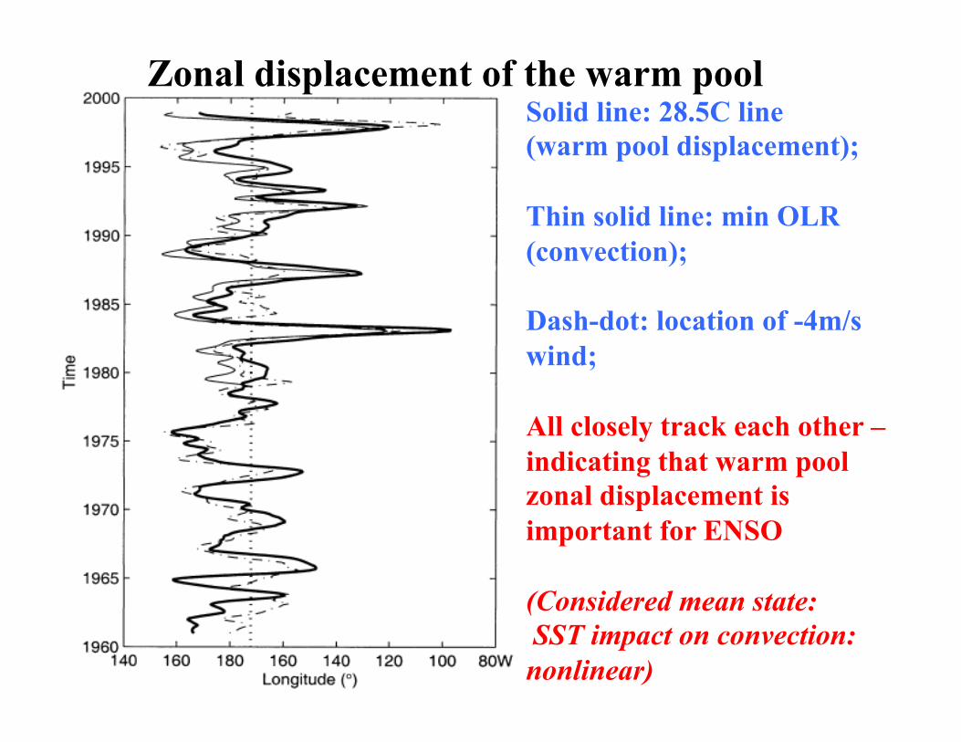
Solid line: 28.5C line (warm pool displacement); Thin solid line: min OLR (convection); Dash-dot: location of -4m/s wind; All closely track each other – indicating that warm pool zonal displacement is important for ENSO (Considered mean state: SST impact on convection: nonlinear)
Zonal displacement of the warm pool
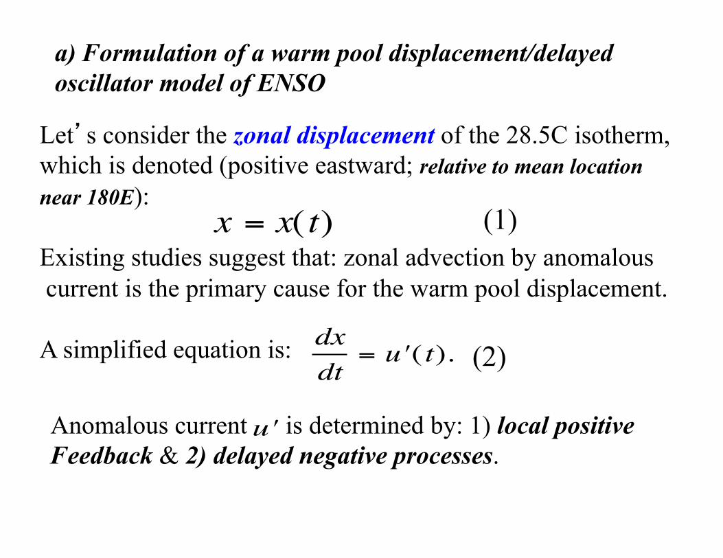
a) Formulation of a warm pool displacement/delayed oscillator model of ENSO
Let’s consider the zonal displacement of the 28.5C isotherm, which is denoted (positive eastward; relative to mean location near 180E): Existing studies suggest that: zonal advection by anomalous current is the primary cause for the warm pool displacement. A simplified equation is: €
x = x( t) (1)
€
dxdt
= " u ( t). (2)
Anomalous current is determined by: 1) local positive Feedback & 2) delayed negative processes.
€
" u
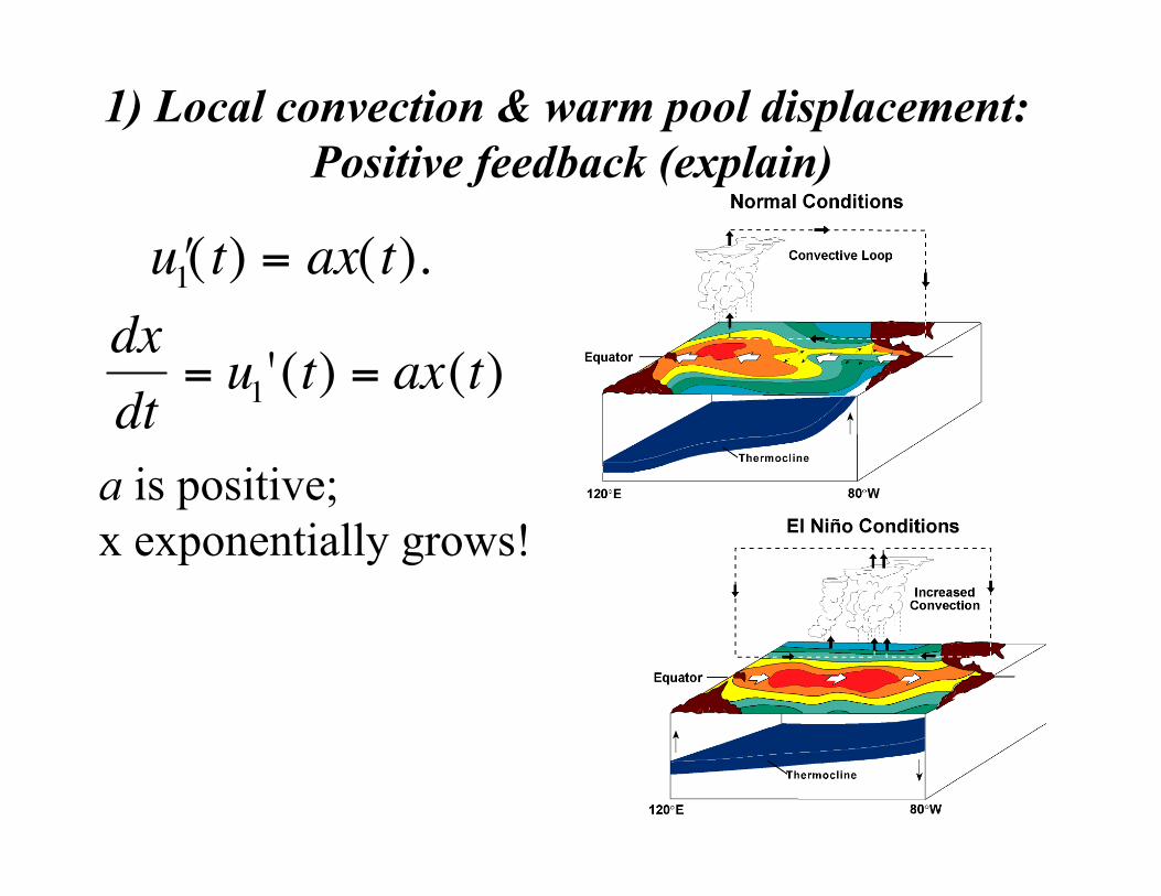
1) Local convection & warm pool displacement: Positive feedback (explain)
€
" u 1( t) = ax(t).
€
dxdt
= u1'(t) = ax(t)
a is positive; x exponentially grows!

Equatorial Kelvin and Rossby waves generated by equatorial westerly wind anomaly
Westerly wind Rossby Kelvin
Sea level anomaly generated by equatorial westerly: Locally forced eastward current anomaly:
€
" u 1
2) Two delayed negative feedback processes
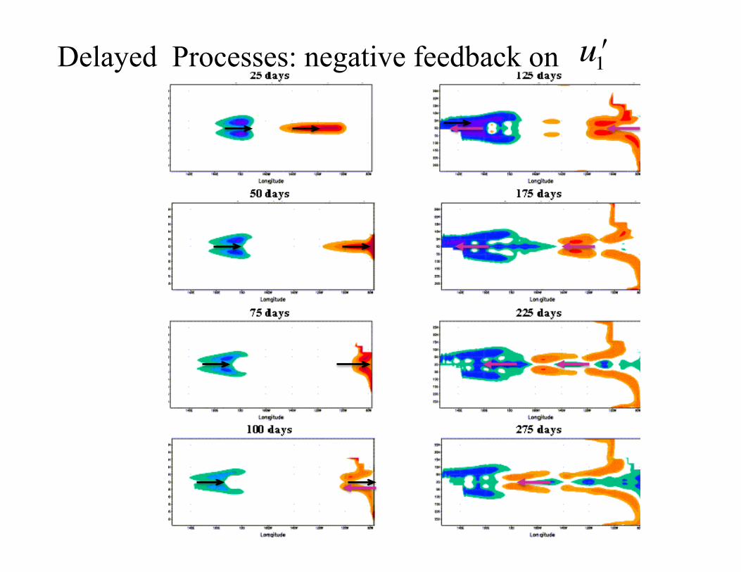
Delayed Processes: negative feedback on
€
" u 1
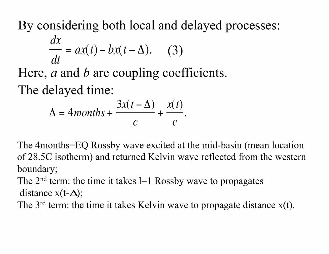
By considering both local and delayed processes:
€
dxdt
= ax( t) − bx(t − Δ).
€
Δ = 4months +3x(t − Δ)
c+x( t)c.
The delayed time:
The 4months=EQ Rossby wave excited at the mid-basin (mean location of 28.5C isotherm) and returned Kelvin wave reflected from the western boundary; The 2nd term: the time it takes l=1 Rossby wave to propagates distance x(t- ); The 3rd term: the time it takes Kelvin wave to propagate distance x(t).
(3)
Here, a and b are coupling coefficients.
€
Δ

€
dxdt
= ax( t) − bx(t − Δ). (3) By considering only the local feedback, the first term on the right hand side of equation (3), the solution is exponentially grow. Physically, this means that a small eastward displacement of the warm pool (small) will cause anomalous deep atmospheric convection, westerly wind anomalies and thus an eastward surface current. This eastward current displaces the warm pool further to the east, generating increased deep atmospheric convection, a stronger westerly wind anomaly, an increased eastward surface current and therefore further eastward warm pool displacement, etc. The delayed part (2nd term on the right hand side) provides negative feedback, limiting the local growth.

Delayed oscillator theory involves three processes (feedbacks). What are they? Critical thinking: If no delay, thus
€
dxdt
= ax( t) − bx(t − Δ).
Δ = 0,
dxdt= ax(t)− bx(t)
instead of
Will ENSO occur?
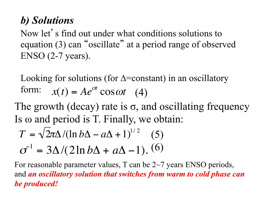
b) Solutions Now let’s find out under what conditions solutions to equation (3) can “oscillate” at a period range of observed ENSO (2-7 years). Looking for solutions (for ∆=constant) in an oscillatory form:
€
x( t) = Aeσt cosωt (4) The growth (decay) rate is σ, and oscillating frequency
Is ω and period is T. Finally, we obtain:
€
T = 2πΔ /(ln bΔ − aΔ +1)1/ 2
€
σ−1 = 3Δ /(2ln bΔ + aΔ −1).(5) (6)
For reasonable parameter values, T can be 2~7 years ENSO periods, and an oscillatory solution that switches from warm to cold phase can be produced!
Physical processes for the “oscillation”: T depends both on ∆ and the time scales 1/a and 1/b of the anomalous advecting flow. Physically, if the negative feedback is sufficiently delayed, there is time for the instability to grow before being damped out by the negative feedback. There is also time, once the damping has overpowered the instability, for the negative feedback to change the sign of x(t), e.g., from positive to negative. The small negative perturbation can then grow and be restrained by delayed negative feedback so that eventually a small positive (eastward) perturbation of the warm pool will occur. => ENSO episodes happen!

Mean EQ Current in the Pacific