Atmospheric Science 4310 / 7310

Atmospheric Thermodynamics

By

Anthony R. Lupo

Syllabus

Atmospheric Thermodynamics ATMS 4310 MTWR 9:00 – 9:50 / 4 credit hrs. Location: 1-120 Agruculture Building Class Ref#: 15505

Instructor: A.R. Lupo Address: 302 E ABNR Building Phone: 88-41638 Fax: 88-45070 Email: lupo@bergeron.snr.missouri.edu or LupoA@missouri.edu Homepage: www.missouri.edu/~lupoa/author.html Class Homepage:www.missouri.edu/~lupoa/atms4310.html

Office hours: MTWR 10:00 – 10:50 302 E ABNR Building

Syllabus

Grading Policy: “Straight” 97 – 100 A+ 77 – 79 C+ 92 – 97 A 72 – 77 C 89 – 92 A- 69 – 72 C- 87 – 89 B+ 67 – 69 D+ 82 – 87 B 62 – 67 D 79 – 82 B- 60 – 62 D- < 60 F

Grading Distribution: Final Exam 20% 2 Tests 40% Homework/Labs 35% Class participation 5% (Note, you WILL lose 1 point for each unexcused

absence, up to 5 points. This IS a half-letter grade, keep that in mind!)

Attendance Policy: “Shouldn’t be an issue!”

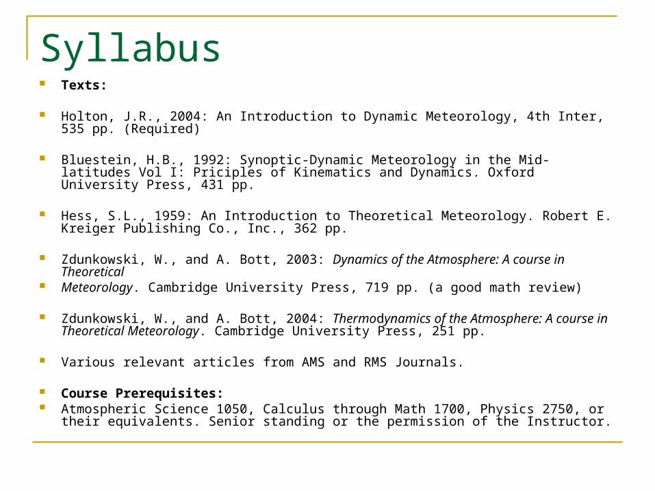
Syllabus Texts:

Holton, J.R., 2004: An Introduction to Dynamic Meteorology, 4th Inter, 535 pp. (Required)

Bluestein, H.B., 1992: Synoptic-Dynamic Meteorology in the Mid-latitudes Vol I: Priciples of Kinematics and Dynamics. Oxford University Press, 431 pp.

Hess, S.L., 1959: An Introduction to Theoretical Meteorology. Robert E. Kreiger Publishing Co., Inc., 362 pp.

Zdunkowski, W., and A. Bott, 2003: Dynamics of the Atmosphere: A course in Theoretical

Meteorology. Cambridge University Press, 719 pp. (a good math review)

Zdunkowski, W., and A. Bott, 2004: Thermodynamics of the Atmosphere: A course in Theoretical Meteorology. Cambridge University Press, 251 pp.

Various relevant articles from AMS and RMS Journals.

Course Prerequisites: Atmospheric Science 1050, Calculus through Math 1700, Physics 2750, or their

equivalents. Senior standing or the permission of the Instructor.

Syllabus

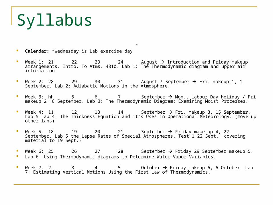
Calendar: “Wednesday is Lab exercise day”

Week 1: 21 22 23 24 August Introduction and Friday makeup arrangements. Intro. To Atms. 4310. Lab 1: The Thermodynamic diagram and upper air information.

Week 2: 28 29 30 31 August / September Fri. makeup 1, 1 September. Lab 2: Adiabatic Motions in the Atmosphere.

Week 3: hh 5 6 7 September Mon., Labour Day Holiday / Fri makeup 2, 8 September. Lab 3: The Thermodynamic Diagram: Examining Moist Processes.

Week 4: 11 12 13 14 September Fri. makeup 3, 15 September,

Lab 5 Lab 4: The Thickness Equation and it’s Uses in Operational Meteorology. (move up other labs)

Week 5: 18 19 20 21 September Friday make up 4, 22 September, Lab 5 the Lapse Rates of Special Atmospheres. Test 1 22 Sept., covering material to 19 Sept.?

Week 6: 25 26 27 28 September Friday 29 September makeup 5.

Lab 6: Using Thermodynamic diagrams to Determine Water Vapor Variables.

Week 7: 2 3 4 5 October Friday makeup 6, 6 October. Lab 7: Estimating Vertical Motions Using the First Law of Thermodynamics.

Syllabus

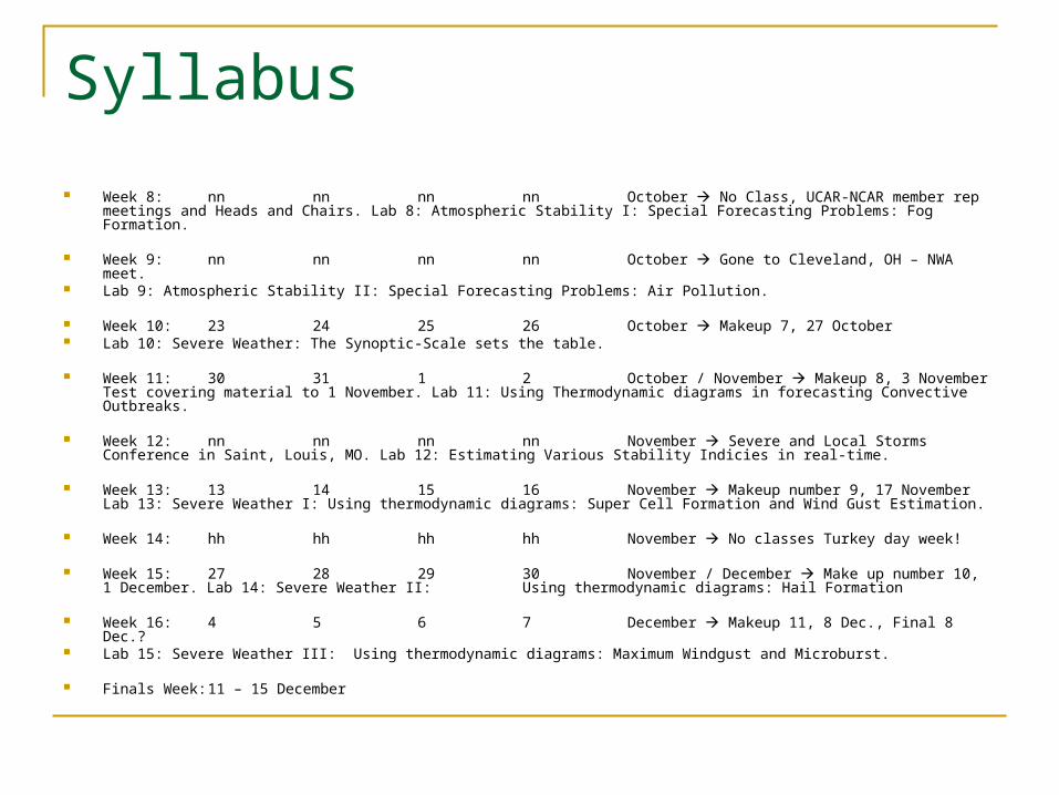
Week 8: nn nn nn nn October No Class, UCAR-NCAR member rep meetings and Heads and Chairs. Lab 8: Atmospheric Stability I: Special Forecasting Problems: Fog Formation.

Week 9: nn nn nn nn October Gone to Cleveland, OH – NWA meet. Lab 9: Atmospheric Stability II: Special Forecasting Problems: Air Pollution.

Week 10: 23 24 25 26 October Makeup 7, 27 October Lab 10: Severe Weather: The Synoptic-Scale sets the table.

Week 11: 30 31 1 2 October / November Makeup 8, 3 November Test covering material to 1 November. Lab 11: Using Thermodynamic diagrams in forecasting Convective Outbreaks.

Week 12: nn nn nn nn November Severe and Local Storms Conference in Saint, Louis, MO. Lab 12: Estimating Various Stability Indicies in real-time.

Week 13: 13 14 15 16 November Makeup number 9, 17 November Lab 13: Severe Weather I: Using thermodynamic diagrams: Super Cell Formation and Wind Gust Estimation.

Week 14: hh hh hh hh November No classes Turkey day week!

Week 15: 27 28 29 30 November / December Make up number 10, 1 December. Lab 14: Severe Weather II: Using thermodynamic diagrams: Hail Formation

Week 16: 4 5 6 7 December Makeup 11, 8 Dec., Final 8 Dec.? Lab 15: Severe Weather III: Using thermodynamic diagrams: Maximum Windgust and Microburst.

Finals Week: 11 – 15 December

Syllabus

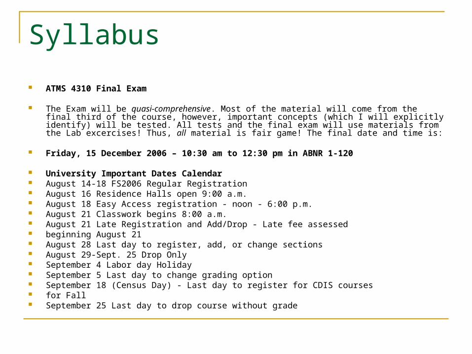
ATMS 4310 Final Exam

The Exam will be quasi-comprehensive. Most of the material will come from the final third of the course, however, important concepts (which I will explicitly identify) will be tested. All tests and the final exam will use materials from the Lab excercises! Thus, all material is fair game! The final date and time is:

Friday, 15 December 2006 – 10:30 am to 12:30 pm in ABNR 1-120

University Important Dates Calendar August 14-18 FS2006 Regular Registration August 16 Residence Halls open 9:00 a.m. August 18 Easy Access registration - noon - 6:00 p.m. August 21 Classwork begins 8:00 a.m. August 21 Late Registration and Add/Drop - Late fee assessed beginning August 21 August 28 Last day to register, add, or change sections August 29-Sept. 25 Drop Only September 4 Labor day Holiday September 5 Last day to change grading option September 18 (Census Day) - Last day to register for CDIS courses for Fall September 25 Last day to drop course without grade

Syllabus

TBA WS2007 Early Registration Appointments October 30 Last day to withdraw from a course - FS2006 November 15 Last day to change divisions November 18 Thanksgiving recess begins, close of day November 27 Classwork resumes, 8:00 a.m. December 8 Fall semester classwork ends December 8 Last day to withdraw from University December 9 Reading Day December 11 Final examinations begin December 15 Fall semester ends at close of day December 15-16 Commencement Weekend *Please note: This calendar is subject to change

Syllabus

Syllabus **

Introductory and Background Material, including a math review (Calculus III)

The Thermodynamics of Dry Air

Hydrostatics

The Thermodynamics of Moist Air

Static Stability and Convection

Vertical Stability, Instability, and Convection*

Cloud Microphysics *

The Thunderstorm and Non-hydrostatic Pressure *

* These topics will be taught if there is time. All Lecture schedules are tentative! ** Students with special need are encouraged to schedule an appointment with me as

soon as possible!

Syllabus

Special Statements:

ADA Statement (reference: MU sample statement)

Please do not hesitate to talk to me!

If you need accommodations because of a disability, if you have emergency medical information to share with me, or if you need special arrangements in case the building must be evacuated, please inform me immediately. Please see me privately after class, or at my office.

Office location: 302 E ABNR Building Office hours : ________________ To request academic accommodations (for example, a notetaker), students must also register with

Disability Services, AO38 Brady Commons, 882-4696. It is the campus office responsible for reviewing documentation provided by students requesting academic accommodations, and for accommodations planning in cooperation with students and instructors, as needed and consistent with course requirements. Another resource, MU's Adaptive Computing Technology Center, 884-2828, is available to provide computing assistance to students with disabilities.

Academic Dishonesty (Reference: MU sample statement and policy guidelines) Any student who commits an act of academic dishonesty is subject to disciplinary action.

Syllabus

The procedures for disciplinary action will be in accordance with the rules and regulations of the University governing disciplinary action.

Academic honesty is fundamental to the activities and principles of a university. All members of the academic community must be confident that each person's work has been responsibly and honorably required, developed, and presented. Any effort to gain an advantage not given to all students is dishonest whether or not the effort is successful. The academic community regards academic dishonesty as an extremely serious matter, with serious consequences that range from probation to expulsion. When in doubt about plagiarism, paraphrasing, quoting, or collaboration, consult the instructor. In cases of suspected plagiarism, the instructor is required to inform the provost. The instructor does not have discretion in deciding whether to do so.

It is the duty of any instructor who is aware of an incident of academic dishonesty in his/her course to report the incident to the provost and to inform his/her own department chairperson of the incident. Such report should be made as soon as possible and should contain a detailed account of the incident (with supporting evidence if appropriate) and indicate any action taken by the instructor with regard to the student's grade. The instructor may include an opinion of the seriousness of the incident and whether or not he/she considers disciplinary action to be appropriate. The decision as to whether disciplinary proceedings are instituted is made by the provost. It is the duty of the provost to report the disposition of such cases to the instructor concerned.

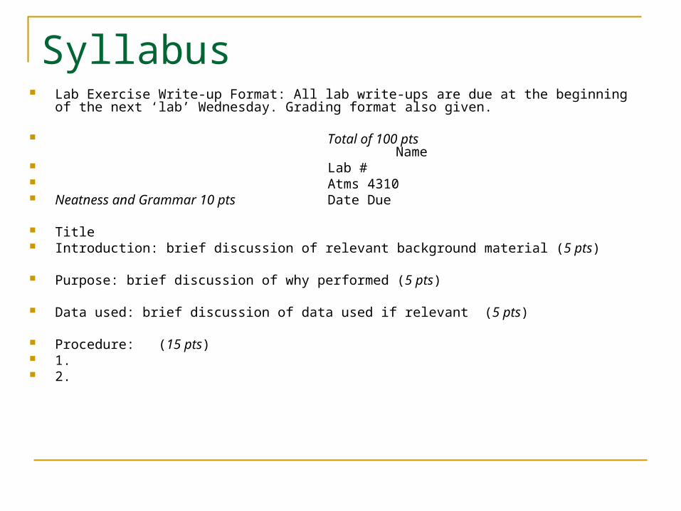
Syllabus Lab Exercise Write-up Format: All lab write-ups are due at the beginning of the next ‘lab’

Wednesday. Grading format also given.

Total of 100 ptsName

Lab # Atms 4310 Neatness and Grammar 10 pts Date Due

Title Introduction: brief discussion of relevant background material (5 pts)

Purpose: brief discussion of why performed (5 pts)

Data used: brief discussion of data used if relevant (5 pts)

Procedure: (15 pts) 1. 2.

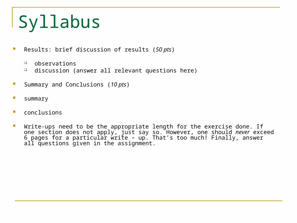
Syllabus Results: brief discussion of results (50 pts)

observations discussion (answer all relevant questions here)

Summary and Conclusions (10 pts)

summary

conclusions

Write-ups need to be the appropriate length for the exercise done. If one section does not apply, just say so. However, one should never exceed 6 pages for a particular write – up. That’s too much! Finally, answer all questions given in the assignment.

Day 1

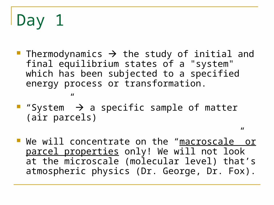
Thermodynamics the study of initial and final equilibrium states of a "system" which has been subjected to a specified energy process or transformation.

“System” a specific sample of matter (air parcels)

We will concentrate on the “macroscale” or parcel properties only! We will not look at the microscale (molecular level) that’s atmospheric physics (Dr. George, Dr. Fox).

Day 1

Day 1

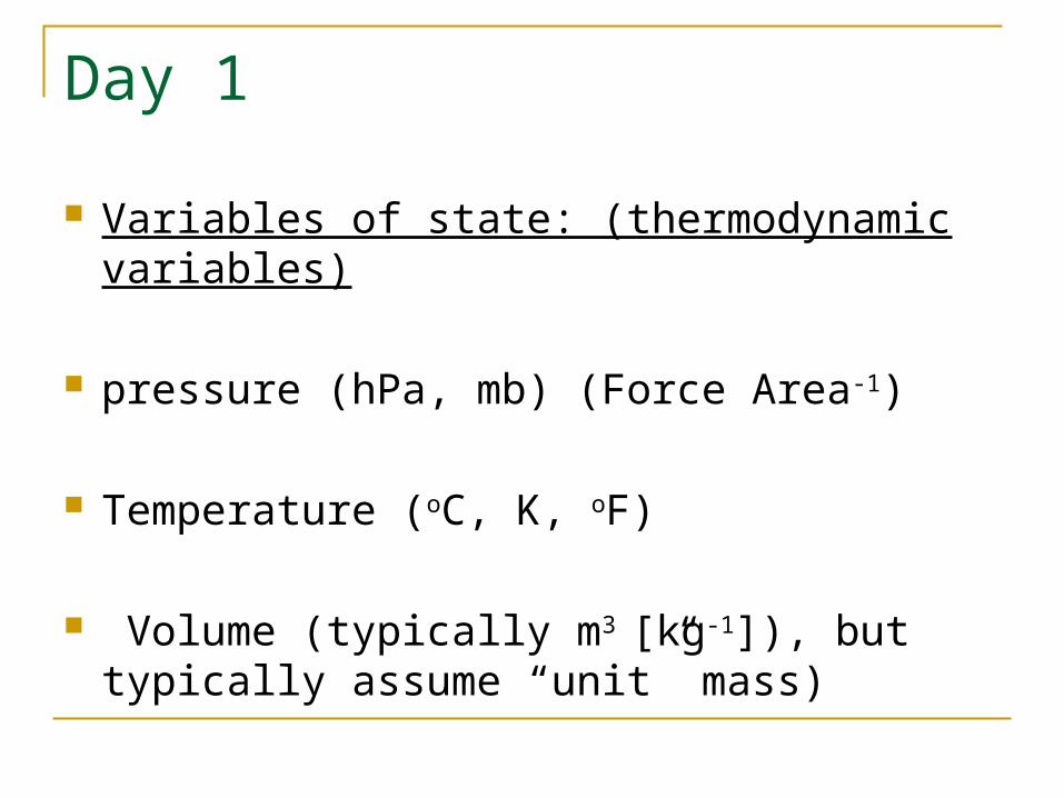
Variables of state: (thermodynamic variables)

pressure (hPa, mb) (Force Area-1)

Temperature (oC, K, oF)

Volume (typically m3 [kg-1]), but typically assume “unit” mass)

Day 1

Laws of thermodynamics:

Equation of State

1st law of thermodynamics (conservation of energy)

2nd law of thermodynamics (entropy) (direction of heat flow) (warm to cold)

We will review Dimensions and Units, and conventions.

Day 1

Atmospheric science derives a set of standard measurements or unit system, such that everyone everywhere will be on the same page.

AMS endorsed the SI (Systeme International) or International system of Units (BAMS, 1974, Aug.)

The basic units are: Length, Mass, Time (meter, m; kilo, kg; second, s)

Day 1

A derived unit combines basic units: example, pressure:

Force /Area = kg m s-2 / m2 = kg m-1 s-2 = Pascals

1000 Pa = 1 kPa = 10 hPa = 10 mb

Temperature (Kelvin, or absolute scale; Celsius (1742) Farenheit (1714)).

Coordinate System: (Cartesian)

Day 1

Coordinate system: tangent to Earth’s surface which is really a sphere (curvature for most applications and approximations can be neglected).

Cartesian coordinates:x,y,z,t => x,y,p,t, or x,y,,t

Could also use natural coordinates: s(treamline),n(normal),z,t

Spherical coordinates r(adius),(longitude),(latitude)

Day 2

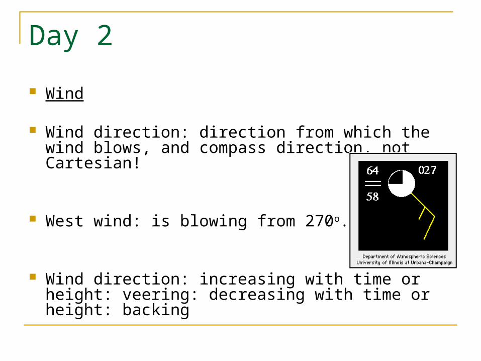
Wind

Wind direction: direction from which the wind blows, and compass direction, not Cartesian!

West wind: is blowing from 270o.

Wind direction: increasing with time or height: veering: decreasing with time or height: backing

Day 2

Remember: Direction of math = 270 – compass (meteorology) direction.

Vector representation in Geophysical Fluid Dynamics

Remember the atmosphere is a fluid, and a fluid is liquid or gas. Thus, the primitive equations will be valid in any atmosphere, terrestrial (extraterrestrial).

Day 2

Scalar quantity A quantity with magnitude only (e.g., wind

speed has units m s-1) (zero order tensor)

Vector (first order Tensor) A quantity with magnitude and direction (e.g., wind velocity)

Day 2

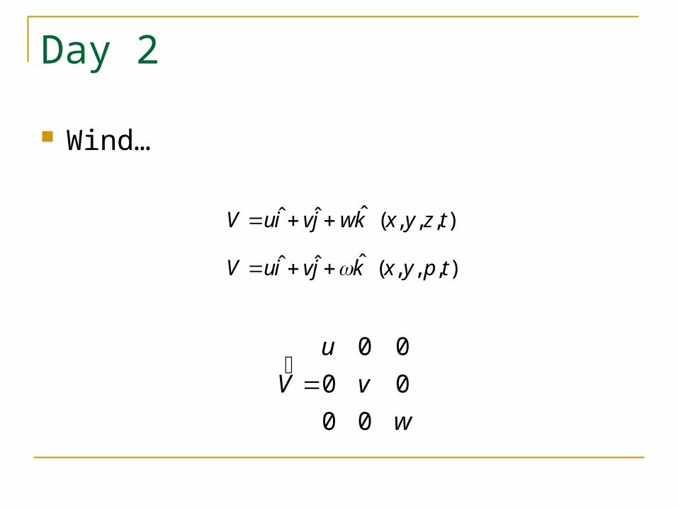
Wind…

),,,(ˆˆˆ

),,,(ˆˆˆ

tpyxkjviuV

tzyxkwjviuV

w

v

u

V

00

00

00

�

Day 2

Dyadic (2nd order Tensor) has a magnitude and two directions!

Example: stress (Force per unit area), where A is the vector of some magnitude equal to the area and in the direction of the normal.

In English: Magnitude, direction (1) of the force, and (2) on which surface applied

Day 2

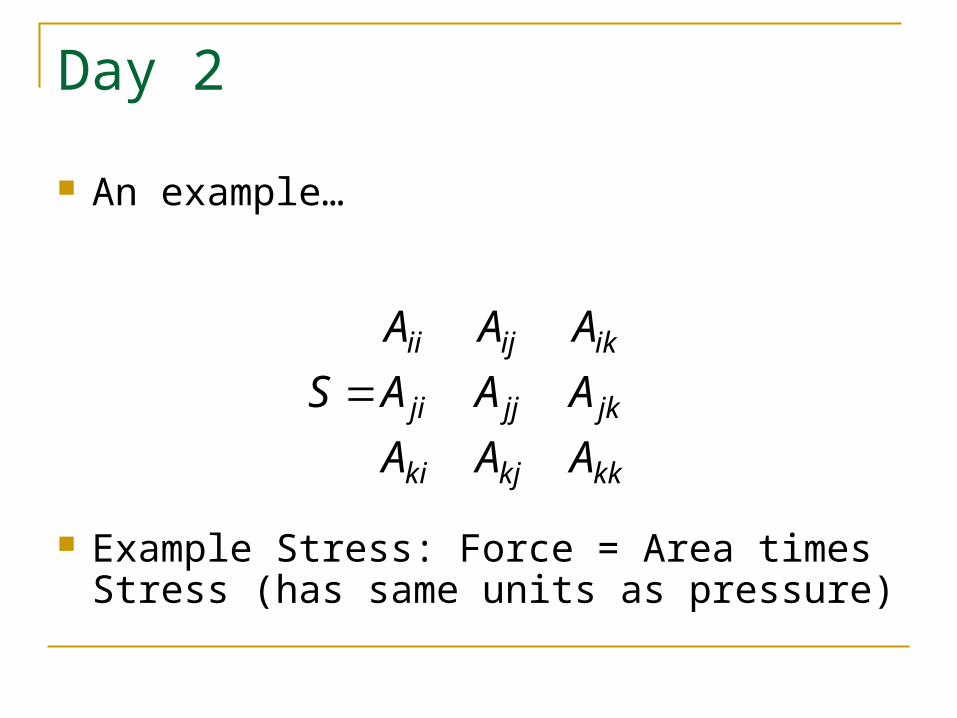
An example…

Example Stress: Force = Area times Stress (has same units as pressure)

kkkjki

jkjjji

ikijii

AAA

AAA

AAA

S

Day 2

Vector Analysis:

Vector Notations:

A A

|A| = magnitude of A

aA ˆ,

Day 2

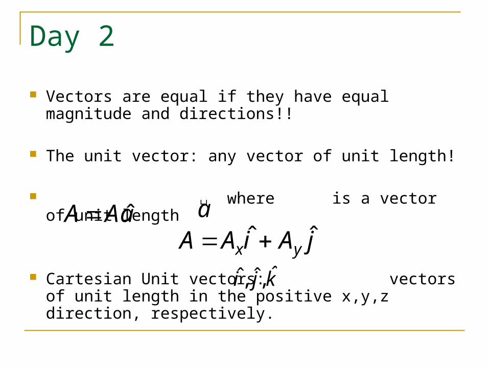
Vectors are equal if they have equal magnitude and directions!!

The unit vector: any vector of unit length!

where is a vector of unit length

Cartesian Unit vectors: vectors of unit length in the positive x,y,z direction, respectively.

jAiAA yxˆˆ

aAA ˆ

a

kji ˆ,ˆ,ˆ

Day 2

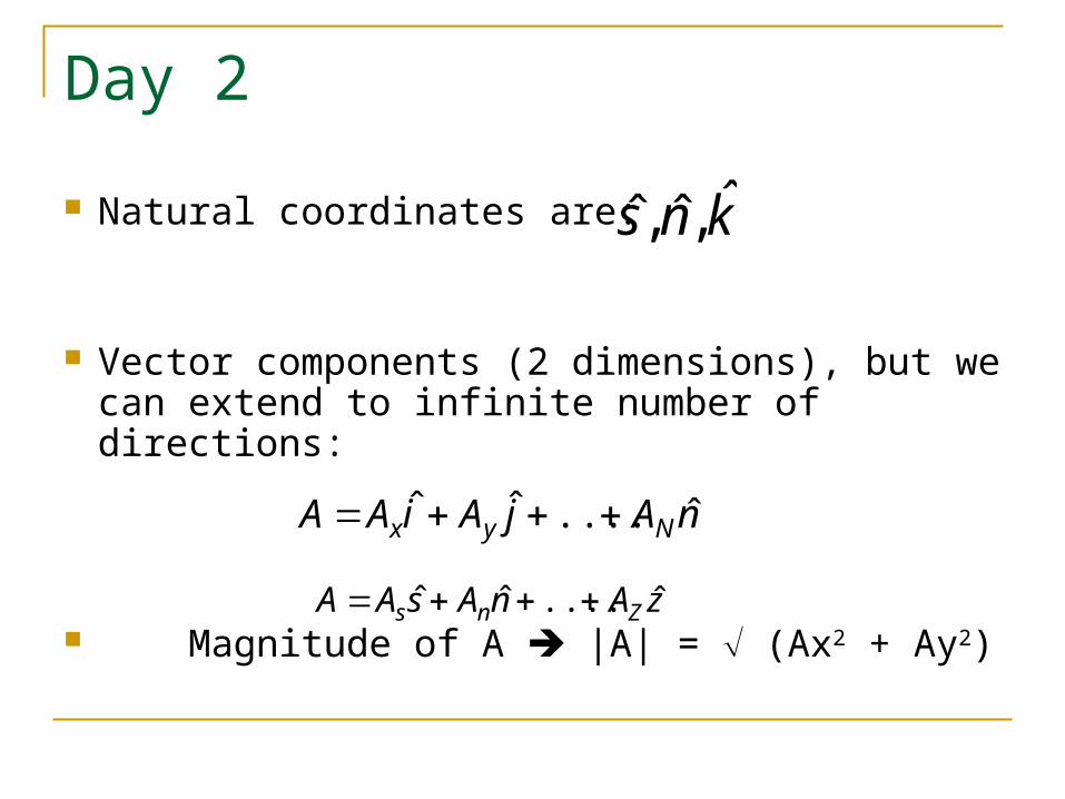
Natural coordinates are:

Vector components (2 dimensions), but we can extend to infinite number of directions:

Magnitude of A |A| = (Ax2 + Ay2)

kns ˆ,ˆ,ˆ

nAjAiAA Nyx ˆ....ˆˆ

zAnAsAA Zns ˆ....ˆˆ

Day 2

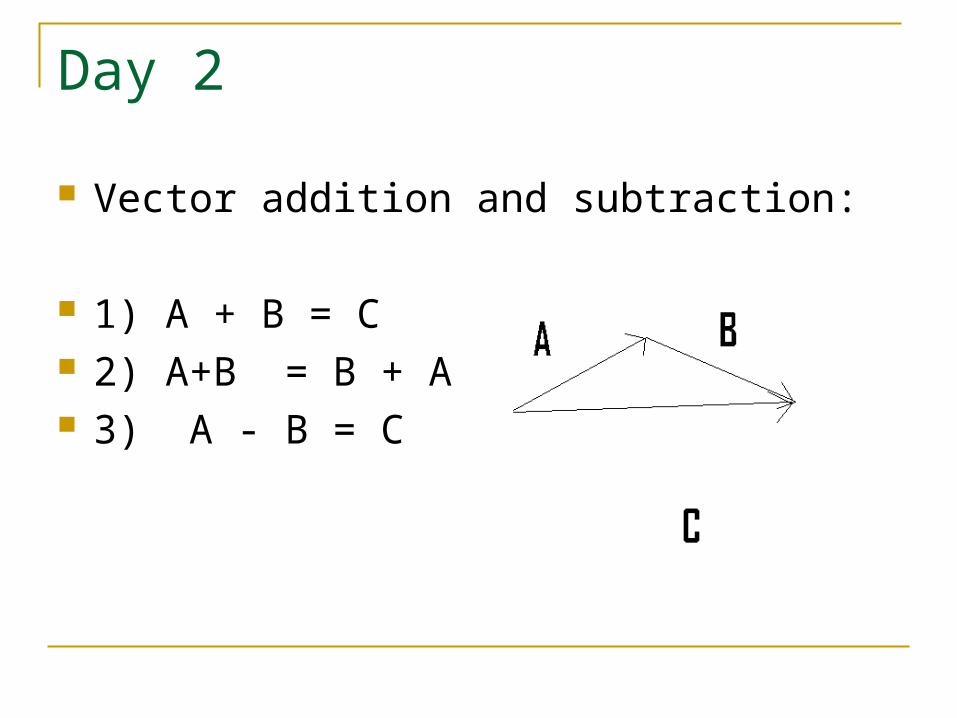
Vector addition and subtraction:

1) A + B = C 2) A+B = B + A = C 3) A - B = C

Day 2

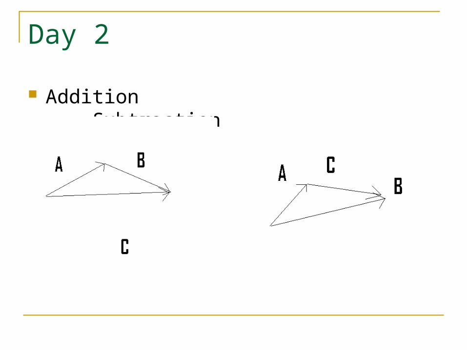
Addition Subtraction

Day 2

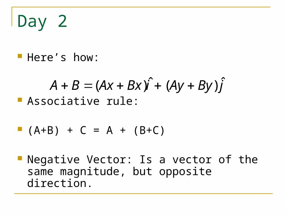
Here’s how:

Associative rule: (A+B) + C = A + (B+C)

Negative Vector: Is a vector of the same magnitude, but opposite direction.

jByAyiBxAxBA ˆ)(ˆ)(

Day 2

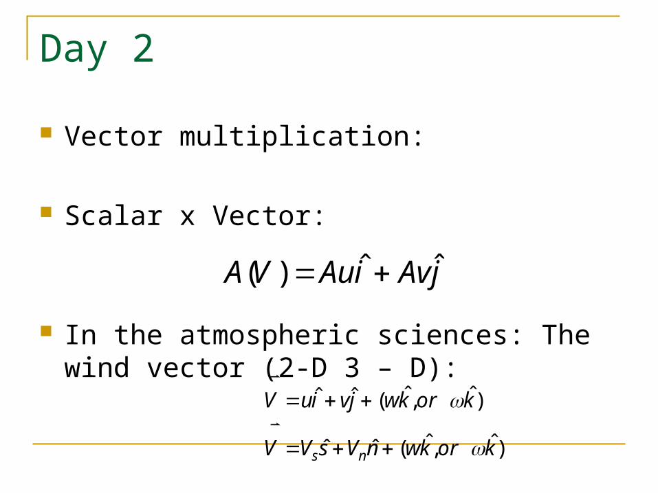
Vector multiplication:

Scalar x Vector:

In the atmospheric sciences: The wind vector (2-D 3 – D):

jAviAuVA ˆˆ)(

)ˆ,ˆ(ˆˆ

)ˆ,ˆ(ˆˆ

korkwnVsVV

korkwjviuV

ns

Day 2 /3

Vector products

The dot product (also the “scalar” or “inner”) product:

A dot B = |A||B|cos()

Physically: The dot product is the PROJECTION of

vector B onto Vector A in direction of A!

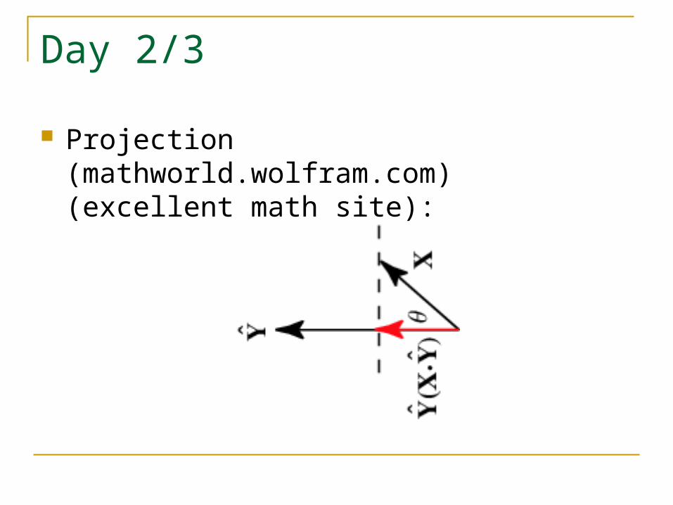
Day 2/3

Projection (mathworld.wolfram.com) (excellent math site):

Day 3

Properties of the Dot Product: commutative

A dot B = B dot A

associative

A dot (B dot C) = (A dot B) dot C

distributive A dot (B + C) = A dot B + A dot C

Day 3

Dot product of perpendicular vector = 0

In order for the dot product to have a value, the B vector must have a component parallel to vector A!

Recall: cos(0o) = 1 and cos(90o) = 0

Thus, i dot j, and j dot k, etc… = 0, and i dot i = 1,

etc…

Day 3

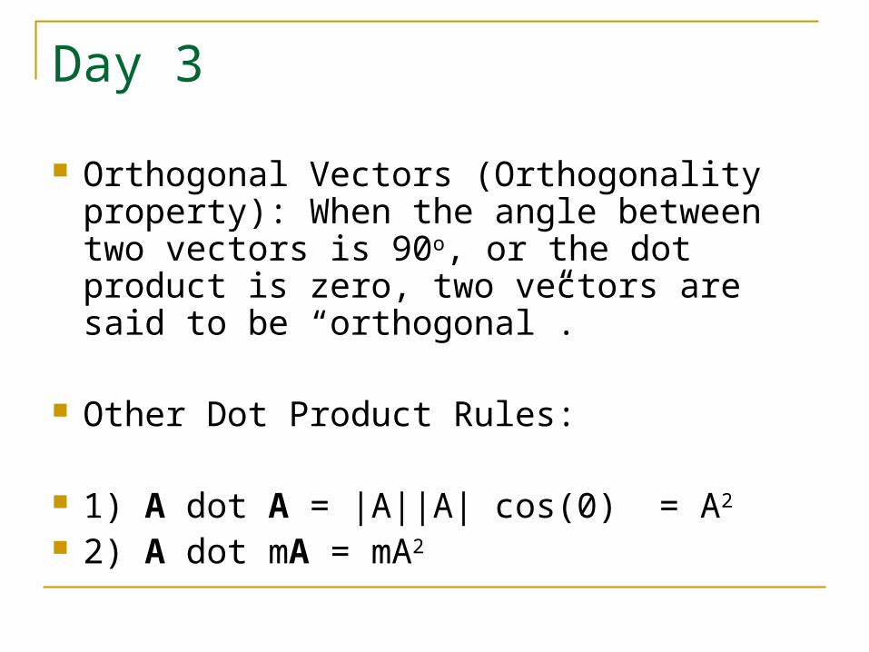
Orthogonal Vectors (Orthogonality property): When the angle between two vectors is 90o, or the dot product is zero, two vectors are said to be “orthogonal”.

Other Dot Product Rules:

1) A dot A = |A||A| cos(0) = A2 2) A dot mA = mA2

Day 3

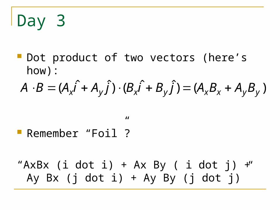
Dot product of two vectors (here’s how):

Remember “Foil”?

“AxBx (i dot i) + Ax By ( i dot j) + Ay Bx (j dot i) + Ay By (j dot j)”

)()ˆˆ()ˆˆ( yyxxyxyx BABAjBiBjAiABA

Day 3

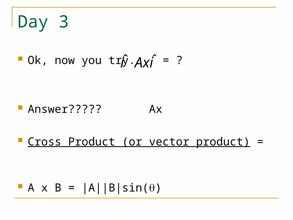
Ok, now you try = ?

Answer????? Ax

Cross Product (or vector product) =

A x B = |A||B|sin()

iAxi ˆˆ

Day 3

What is it (again courtesy of Mathworld site)?

Day 3

Einstien notation – permutation:

Q: "What do you get when you cross a mountain-climber with a mosquito?"

A: "Nothing: you can't cross a scaler with a vector,"

Q: "What do you get when you cross an elephant and a grape?"

A: "Elephant grape sine-of-theta."

                           

Day 3

The cross product of two vectors is a third vector that is mutually perpendicular to the two vectors and the plane containing these vectors.

Q: Remember your Physics?

The positive direction of A x B may be determined by the “right hand (or corkscrew)” rule. Just curl your fingers from A to B, and your right thumb (vector C) is the result! (“ayyyy”)

Day 3

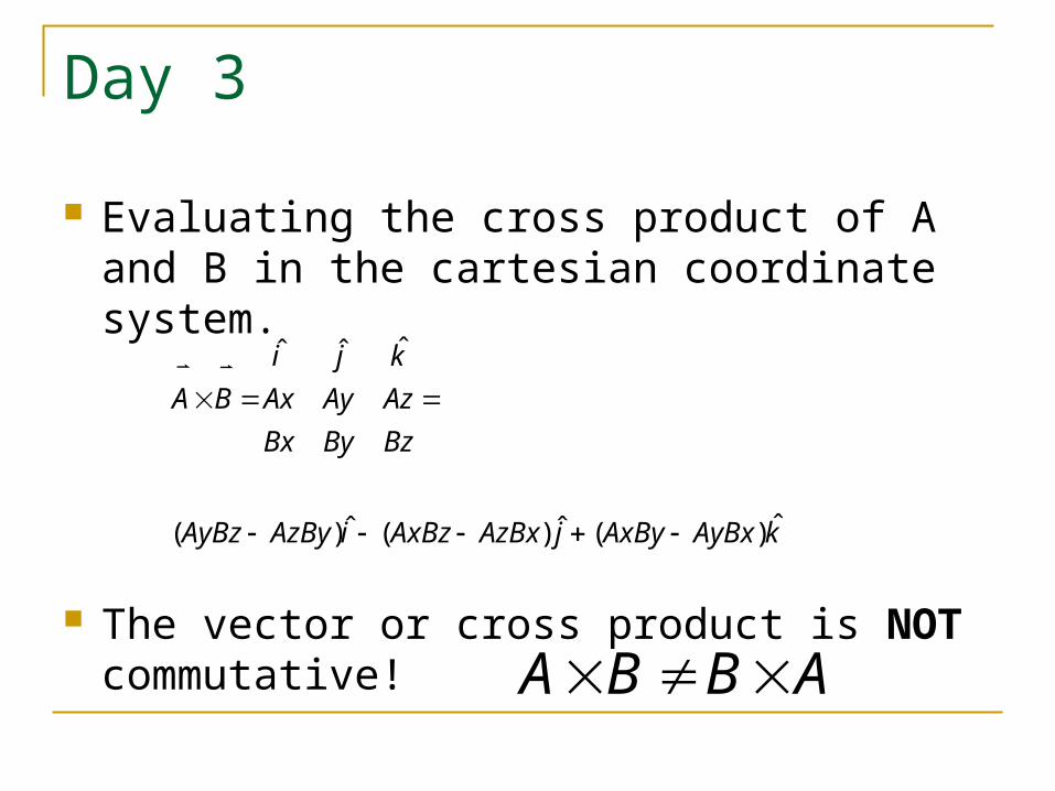
Evaluating the cross product of A and B in the cartesian coordinate system.

The vector or cross product is NOT commutative!

kAyBxAxByjAzBxAxBziAzByAyBz

BzByBx

AzAyAx

kji

BA

ˆ)(ˆ)(ˆ)(

ˆˆˆ

ABBA

Day 3

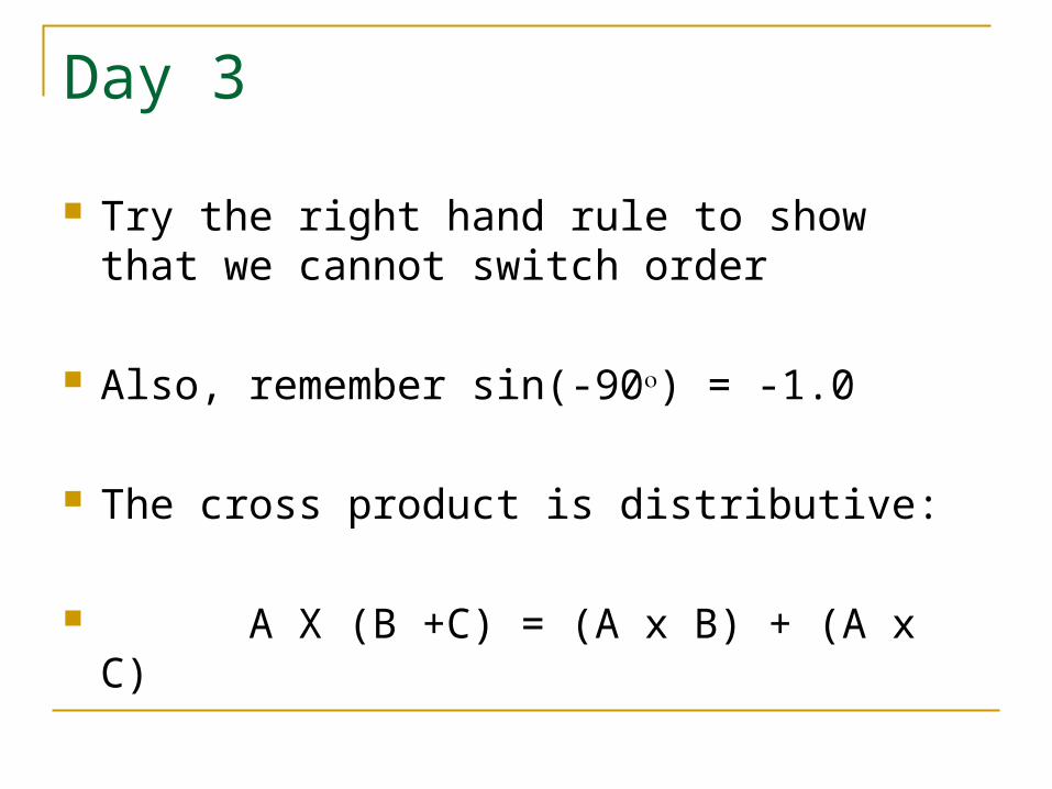
Try the right hand rule to show that we cannot switch order

Also, remember sin(-90) = -1.0

The cross product is distributive:

A X (B +C) = (A x B) + (A x C)

Day 3/4

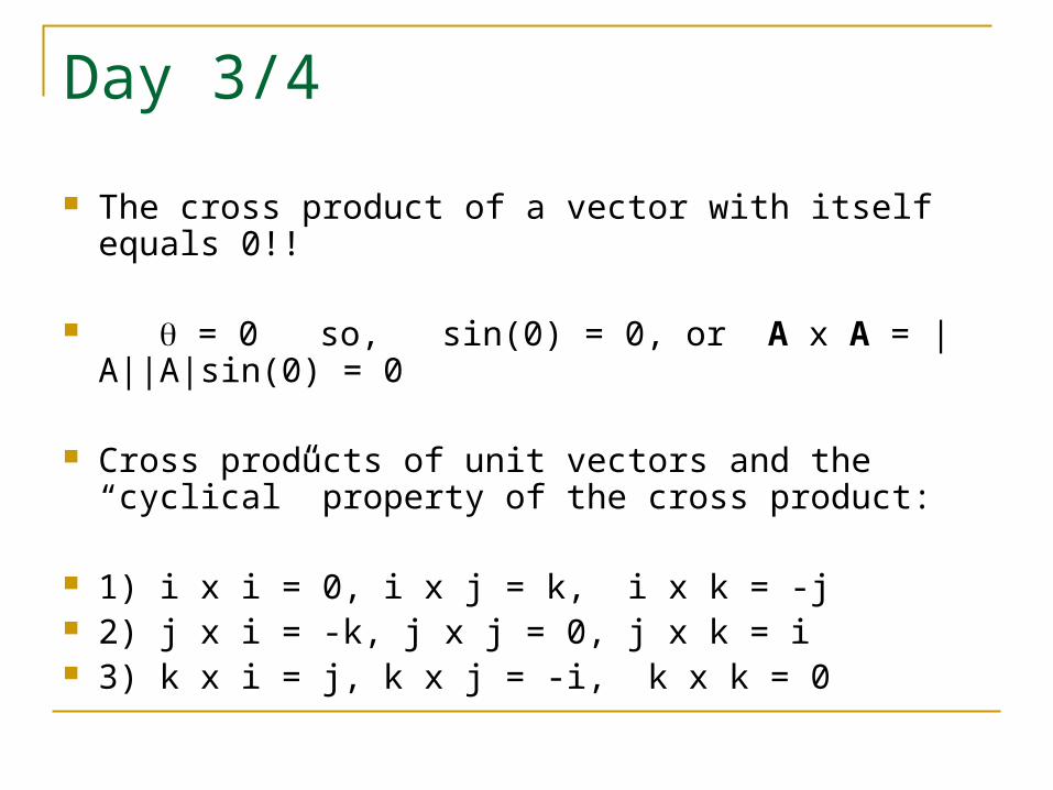
The cross product of a vector with itself equals 0!!

= 0 so, sin(0) = 0, or A x A = |A||A|sin(0) = 0

Cross products of unit vectors and the “cyclical” property of the cross product:

1) i x i = 0, i x j = k, i x k = -j 2) j x i = -k, j x j = 0, j x k = i 3) k x i = j, k x j = -i, k x k = 0

Day 4

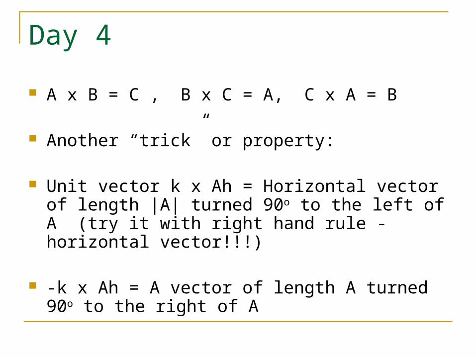
A x B = C , B x C = A, C x A = B

Another “trick” or property:

Unit vector k x Ah = Horizontal vector of length |A| turned 90o to the left of A (try it with right hand rule - horizontal vector!!!)

-k x Ah = A vector of length A turned 90o to the right of A

Day 4

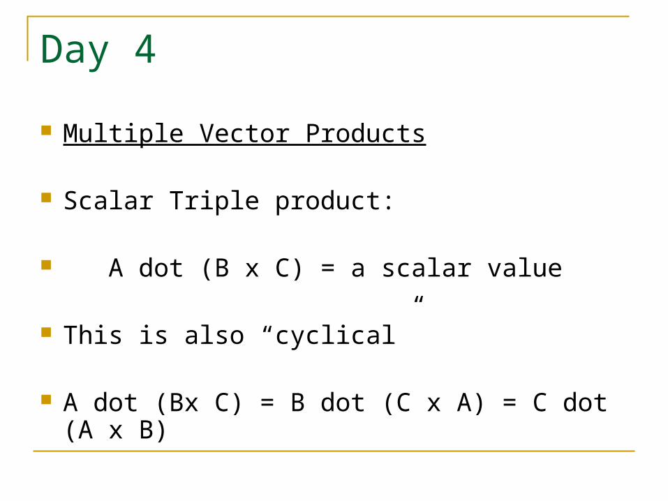
Multiple Vector Products

Scalar Triple product:

A dot (B x C) = a scalar value

This is also “cyclical”

A dot (Bx C) = B dot (C x A) = C dot (A x B)

Day 4

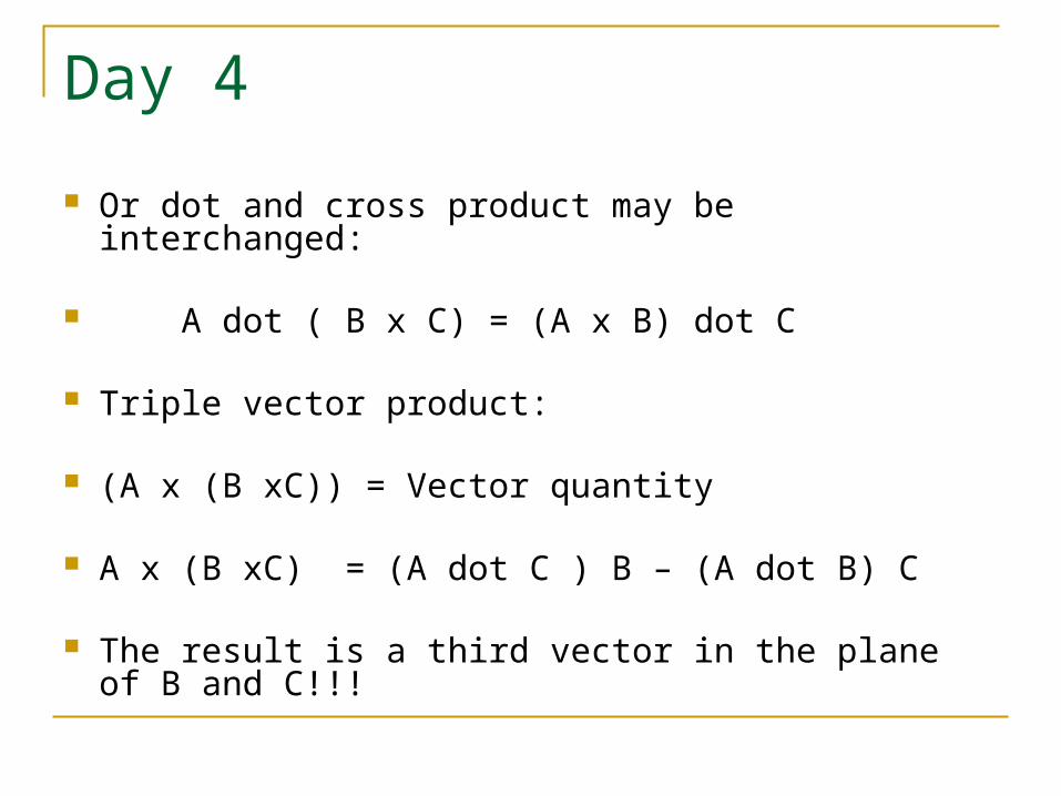
Or dot and cross product may be interchanged:

A dot ( B x C) = (A x B) dot C

Triple vector product:

(A x (B xC)) = Vector quantity

A x (B xC) = (A dot C ) B – (A dot B) C

The result is a third vector in the plane of B and C!!!

Day 4

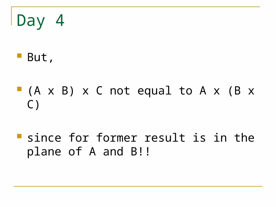
But,

(A x B) x C not equal to A x (B x C)

since for former result is in the plane of A and

B!!

Day 4/5

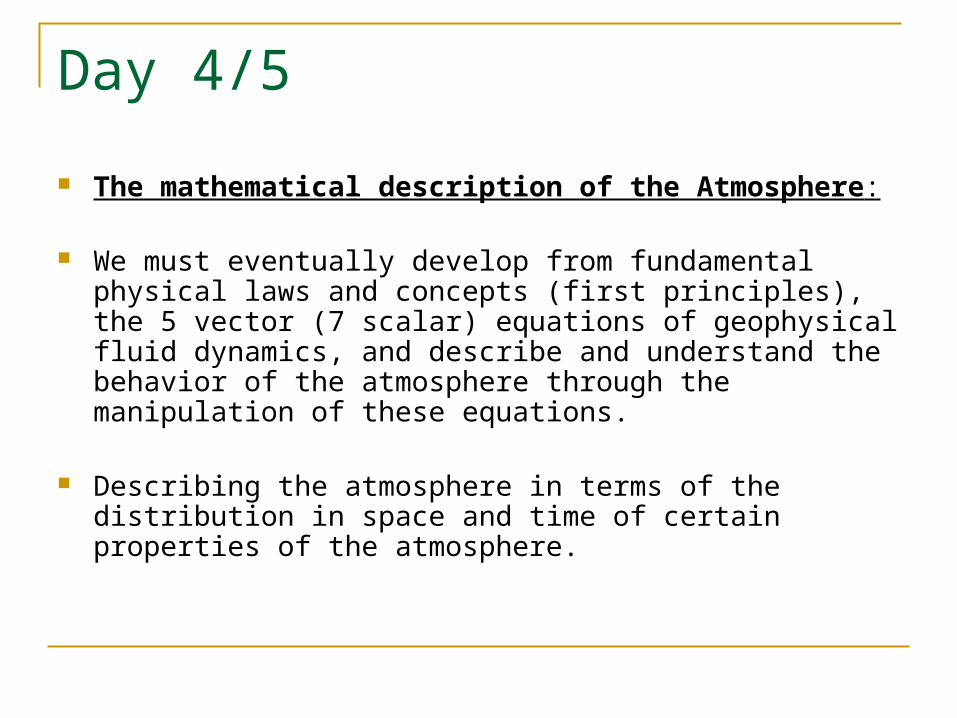
The mathematical description of the Atmosphere:

We must eventually develop from fundamental physical laws and concepts (first principles), the 5 vector (7 scalar) equations of geophysical fluid dynamics, and describe and understand the behavior of the atmosphere through the manipulation of these equations.

Describing the atmosphere in terms of the distribution in space and time of certain properties of the atmosphere.

Day 5

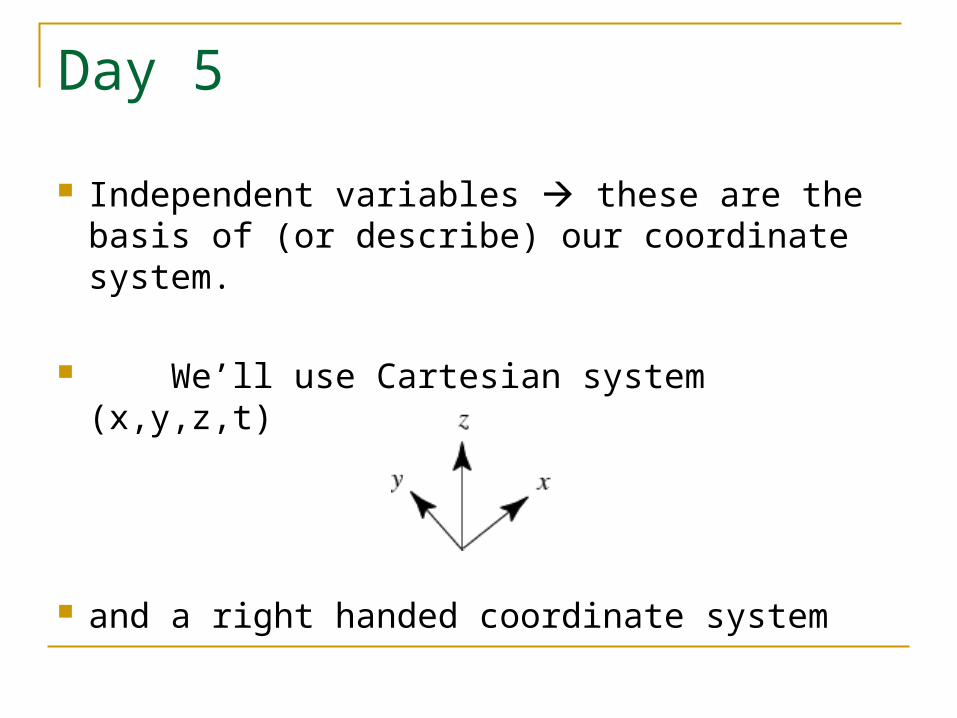
Independent variables these are the basis of (or describe) our coordinate system.

We’ll use Cartesian system (x,y,z,t)

and a right handed coordinate system

Day 5

Dependent variables depend on your position in space and time, and can be described as a function of the independent variables.

In atmospheric science: u,v,T,,P,w,or

Example: u(x,y,z,t)

Day 5

Invariance A quantity that does not change if measured in a different coordinate system

e.g., “rotationally” invariant quantities that do not change even if coordinate system rotates

Q: Which variable might be rotationally invariant?

A: T(x,y,z,t) = T(x’,y’z’,t)

Galilean invariant quantities that do not change even if coordinate system is moving horizontally

Day 5

Important Definintion!

Conserved a quantity that does not

change with time. (e.g., Potential Temperature and adiabatic motions)

Conservation the change in some quantity with time equals 0!

Day 5

Conservation = steady state = balance (between sources and sinks!)

where Q = any quantity

kssourcedt

dQsin0

Day 5

The derivative (A review)

Let take a quantity: Q(x,y,z,t)

Now one needs to take the Total Derivative. In order to do this, we must use the “Chain Rule!” Remember this?

Day 5

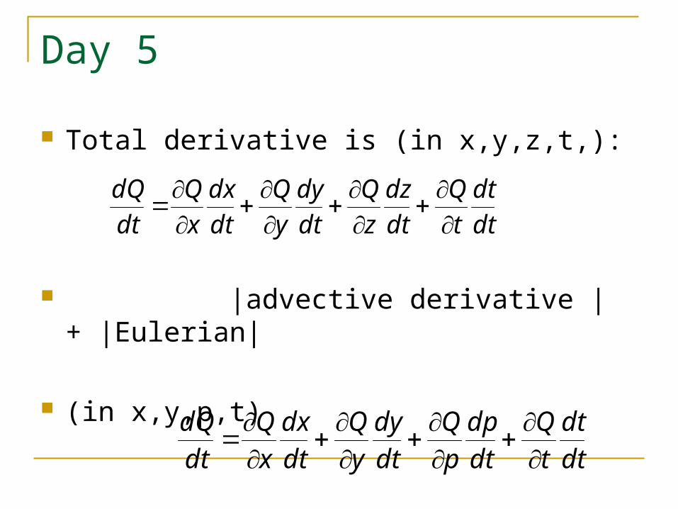
Total derivative is (in x,y,z,t,):

|advective derivative | + |Eulerian|

(in x,y,p,t)

dt

dt

t

Q

dt

dz

z

Q

dt

dy

y

Q

dt

dx

x

Q

dt

dQ

dt

dt

t

Q

dt

dp

p

Q

dt

dy

y

Q

dt

dx

x

Q

dt

dQ

Day 5

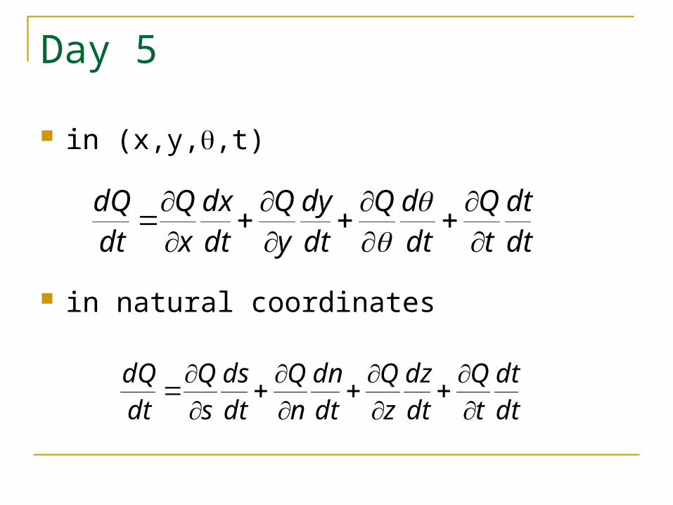
in (x,y,,t)

in natural coordinates

dtdt

tQ

dtdQ

dtdy

yQ

dtdx

xQ

dtdQ

dt

dt

t

Q

dt

dz

z

Q

dt

dn

n

Q

dt

ds

s

Q

dt

dQ

Day 5

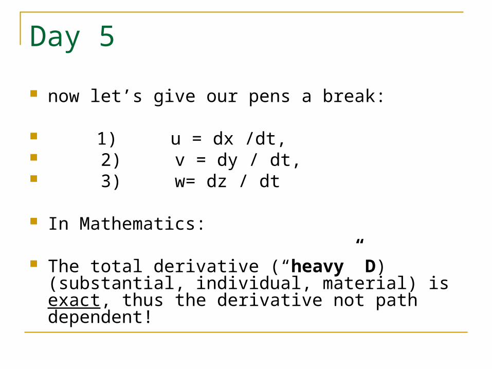
now let’s give our pens a break:

1) u = dx /dt, 2) v = dy / dt, 3) w= dz / dt

In Mathematics:

The total derivative (“heavy” D) (substantial, individual, material) is exact, thus the derivative not path dependent!

Day 5

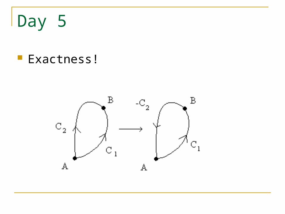
Exactness!

Day 5

But, if path dependent, total derivative has no meaning, and we write with a small “d”.

If path dependent, then the process is sensitive to the initial starting place and it corresponds to (generally) one outcome.

But I, like most atmospheric scientists use the notation “d” for a total derivative regardless.

Day 5

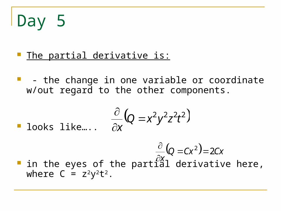
The partial derivative is:

- the change in one variable or coordinate w/out regard to the other components.

looks like…..

in the eyes of the partial derivative here, where C = z2y2t2.

2222 tzyxQx

CxCxQx

22

Day 5/6

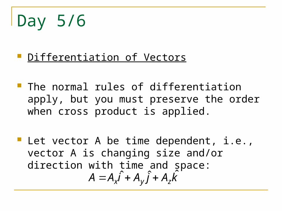
Differentiation of Vectors

The normal rules of differentiation apply, but you must preserve the order when cross product is applied.

Let vector A be time dependent, i.e., vector A is changing size and/or direction with time and space:

kAjAiAA zyxˆˆˆ

Day 6

If our coordinate system is not changing (i.e., i,j,k = constant)….

then Ax,Ay,Az change (of course!)

(oh, you fill in the rest!)...ˆ iDt

DAx

Dt

AD

Day 6

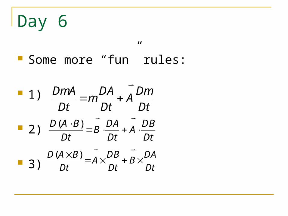
Some more “fun” rules:

1)

2)

3)

DtDm

ADtAD

mDtADm

DtBD

ADtAD

BDtBAD

)(

DtAD

BDtBD

ADt

BAD

)(

Day 6

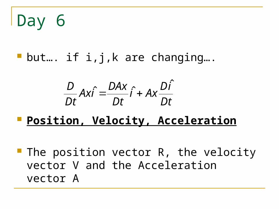
but…. if i,j,k are changing….

Position, Velocity, Acceleration

The position vector R, the velocity vector V and the Acceleration vector A

Dt

iDAxi

Dt

DAxiAx

Dt

D ˆˆˆ

Day 6

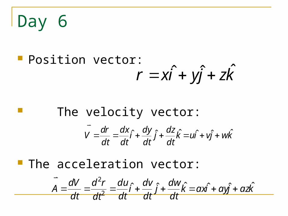
Position vector:

The velocity vector:

The acceleration vector:

kzjyixr ˆˆˆ

kwjviukdt

dzj

dt

dyi

dt

dx

dt

rdV ˆˆˆˆˆˆ

kazjayiaxkdt

dwj

dt

dvi

dt

du

dt

rd

dt

VdA ˆˆˆˆˆˆ

2

2

Day 6

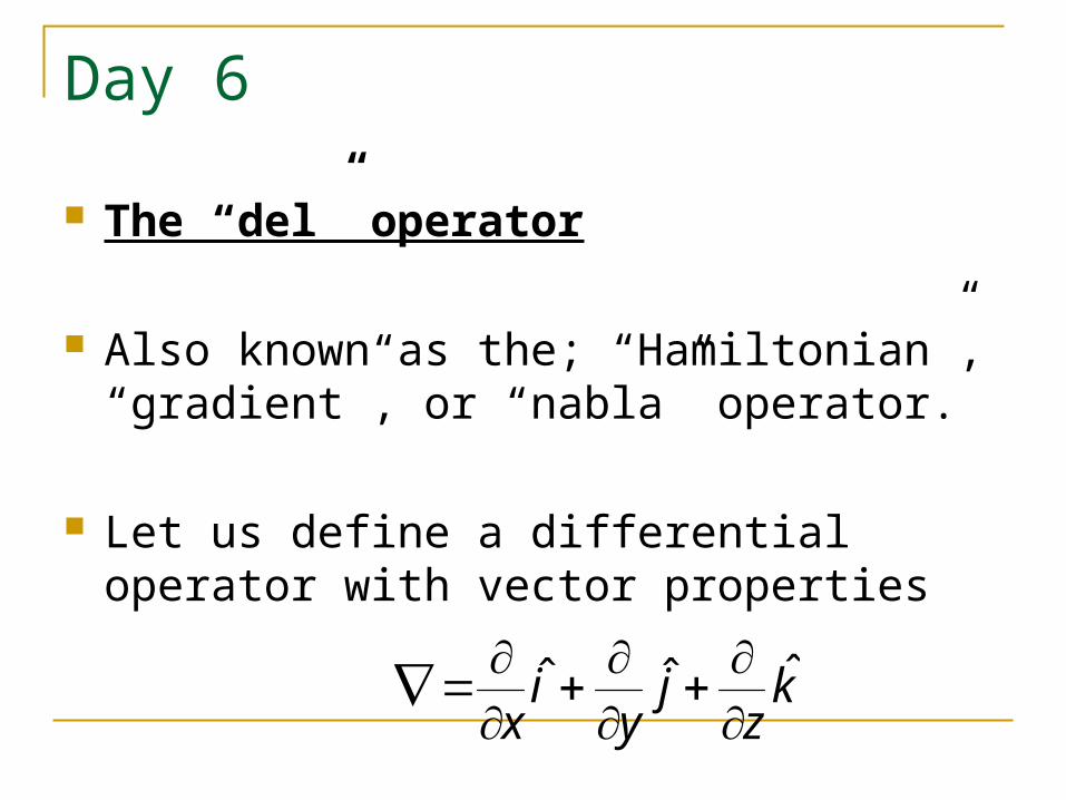
The “del” operator

Also known as the; “Hamiltonian”, “gradient”, or “nabla” operator.

Let us define a differential operator with vector properties

kz

jy

ix

ˆˆˆ

Day 6

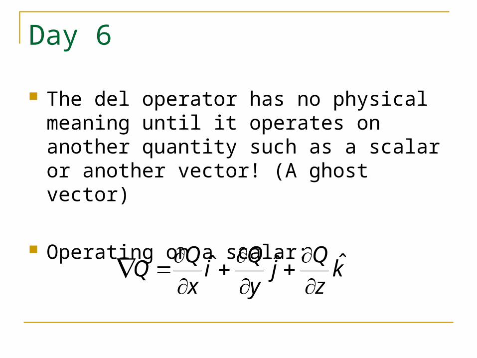
The del operator has no physical meaning until it operates on another quantity such as a scalar or another vector! (A ghost vector)

Operating on a scalar:

kz

Qj

y

Qi

x

QQ ˆˆˆ

Day 6

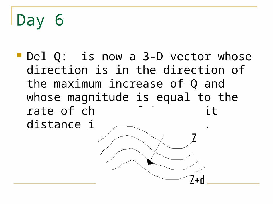
Del Q: is now a 3-D vector whose direction is in the direction of the maximum increase of Q and whose magnitude is equal to the rate of change of Q per unit distance in that direction.

Day 6

Del Q in normal (perpendicular to lines of Q). On a 2 – D surface is perpendicular to Q isolines.

Then in “plane” English: delQ is simply the slope of Q on some planar surface. The first derivative in space (slope) is analogous to the first derivative in time (velocity).

Day 6/7

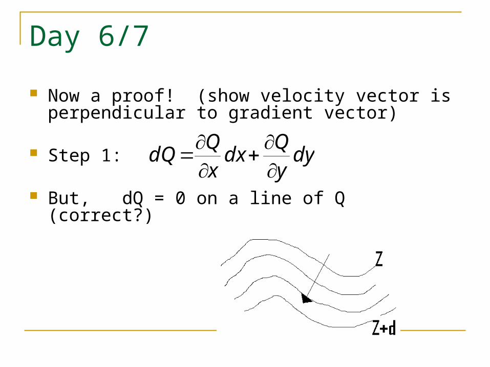
Now a proof! (show velocity vector is perpendicular to gradient vector)

Step 1:

But, dQ = 0 on a line of Q (correct?)

dyyQ

dxxQ

dQ

Day 7

Now we know that;

a) each point of a surface of constant Q can be defined by the position vector.

b) then on a Q surface dr (or V), must be on the surface of Q, so dr must lie on the Q surface.

Day 7

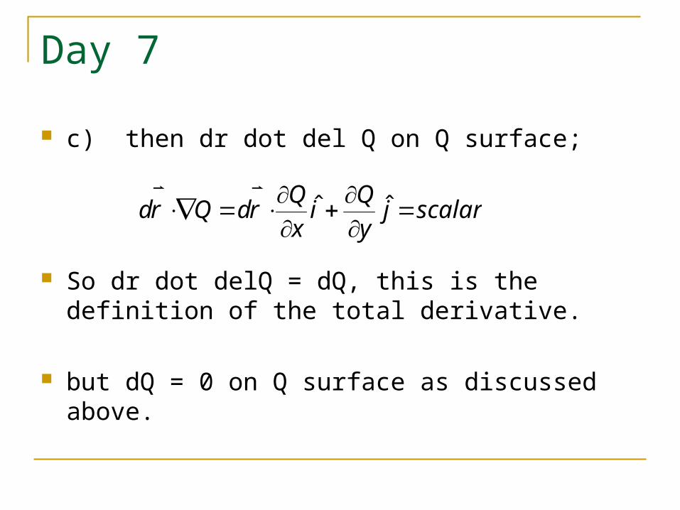
c) then dr dot del Q on Q surface;

So dr dot delQ = dQ, this is the definition of the total derivative.

but dQ = 0 on Q surface as discussed above.

scalarjy

Qi

x

QrdQrd

ˆˆ

Day 7

Therefore since dr and delQ separately are not 0, but their dot product IS 0, they must be perpendicular (or orthogonal)!!!

Furthermore, we know that delQ was perpendicular to lines of Q, thus dr or Velocity, must be parallel to lines of Q!

Point proved!

Day 7

Advection of a scalar quantity

3-D transport of some quantity:

In Atms Sci, in (x,y,p,t) coordinates, advection and flux are equivalent.

Day 7

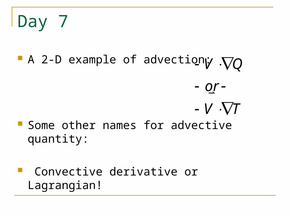
A 2-D example of advection:

Some other names for advective quantity:

Convective derivative or Lagrangian!

TV

or

QV

Day 7

Two definitions:

Lagrangian measurement measurement that moves with the flow (“goes with the flow”)

Eulerian measurement at a stationary point

Important Concept!!

If Q is conserved or a conserved property (invariant with time) time derivative = 0. We also call this “steady state”.

Day 7

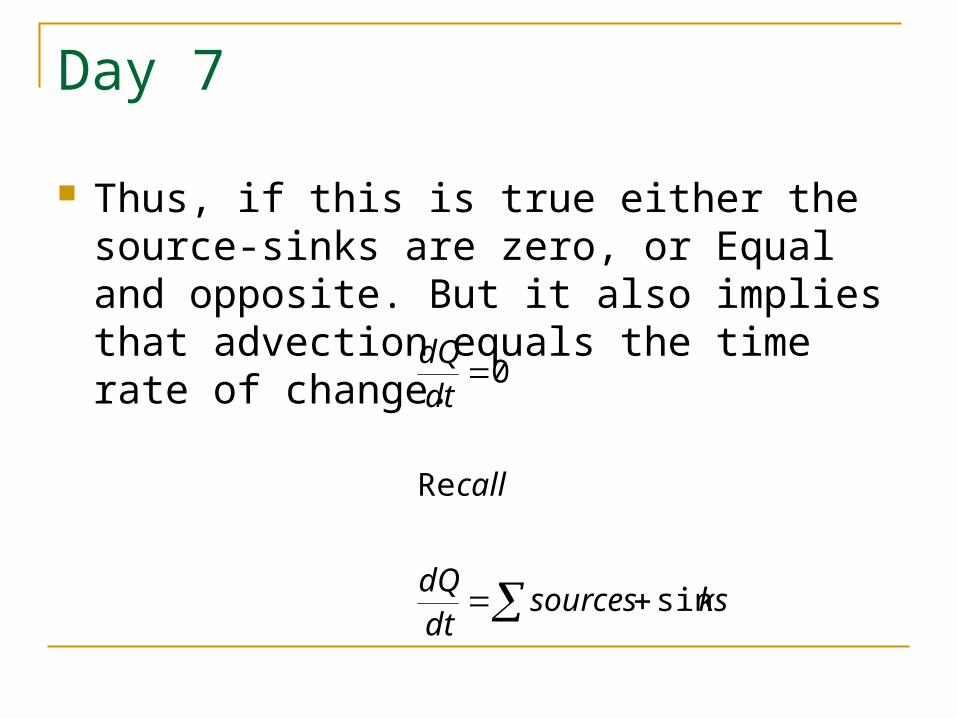
Thus, if this is true either the source-sinks are zero, or Equal and opposite. But it also implies that advection equals the time rate of change.

kssourcesdtdQ

call

dtdQ

sin

Re

0

Day 7

- or –

where Q = Any variable, vector or scalar!

QVtQ

Day 7

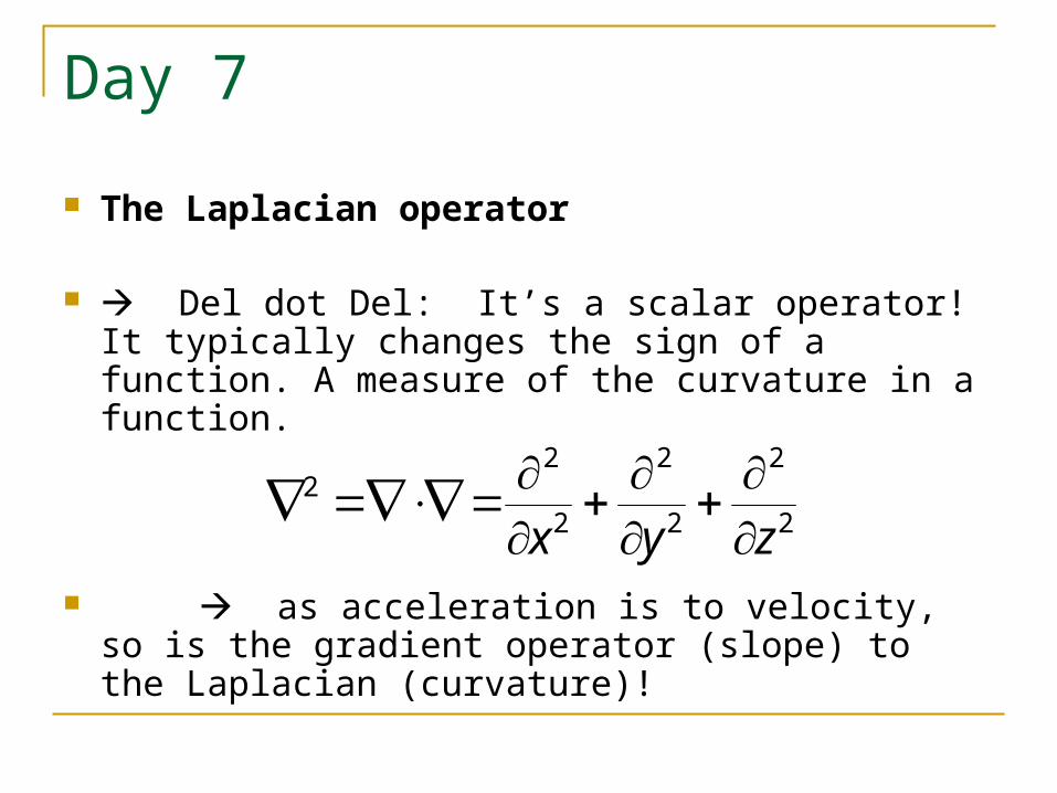
The Laplacian operator

Del dot Del: It’s a scalar operator! It typically changes the sign of a function. A measure of the curvature in a function.

as acceleration is to velocity, so is the gradient operator (slope) to the Laplacian (curvature)!

2

2

2

2

2

22

zyx

Day 7

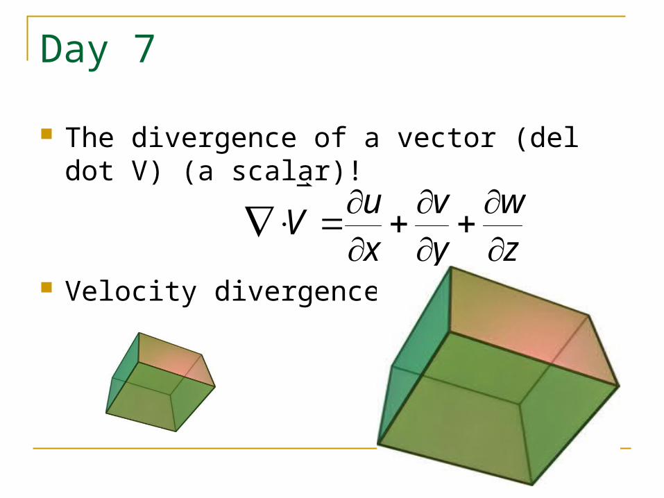
The divergence of a vector (del dot V) (a scalar)!

Velocity divergence:

zw

yv

xu

V

Седьмой Дни

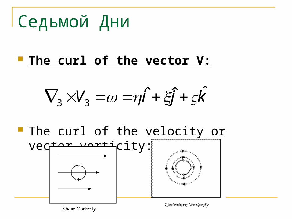
The curl of the vector V:

The curl of the velocity or vector vorticity:

kjiV ˆˆˆ33

Day 7

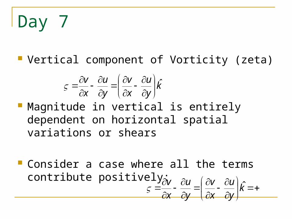
Vertical component of Vorticity (zeta)

Magnitude in vertical is entirely dependent on horizontal spatial variations or shears

Consider a case where all the terms contribute positively:

kyu

xv

yu

xv ˆ

k

yu

xv

yu

xv ˆ

Day 7/8

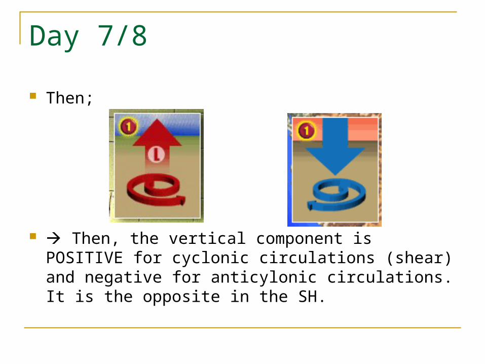
Then;

Then, the vertical component is POSITIVE for cyclonic circulations (shear) and negative for anticylonic circulations. It is the opposite in the SH.

Day 8

Rotational Vectors and vectors in Rotation

Definition of the rotational vector (omega - ) rotational vector has a direction along the axis, positive in the sense of the Right hand rule, and it’s magnitude, omega ||, is porportional to the angular velocity of the rotating system. (ang. Vel.= radians/sec)

The rate of change of a vector A of constant magnitude due to it’s changing direction produced by rotation (omega - )

Day 8

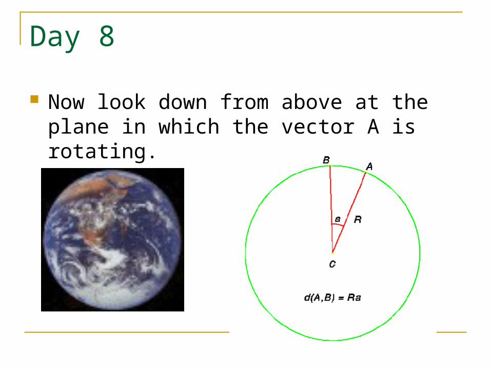
Now look down from above at the plane in which the vector A is rotating.

Day 8

The magn. Or length of A = A and for small angle

Recall from Geometery:

A = A sin() since for small angles tan = opp. /

adj. Or opp. = adj. tan

Day 8

So, (now include delta t)

A/ t = A sin() ( / t)

And as t goes to 0

dA/dt = A sin()(d /dt)

Day 8

But d /dt = omega (the angular velocity) So;

dA/dt = A sin ()

Then we need to;

redefine as since we’re talking about earth!

recall our definition of the cross product!!! ( x A)

Day 7

Thus the magnitude of DA/dt = DA/dt equals the mangitudes of x A!!

dA/dt = xA!

Day 8

Direction of dA/dt and x A

Since ( x A is mutually perpendicular to and A as is DA/dt, and is positive in the same direction the two vectors DA/dt and x A are equal vectors!

Thus for A of constant magnitude dA/dt = x A

Day 8

The rate of change of vector A in a fixed (absolute) coordinate system vs. a rotating coordinate system. (“Fixed” and “absolute” are not good news – we can’t do this in practice (in real atms.)).

Atms example: coriolis force!!

dV/dt = x V

Day 8

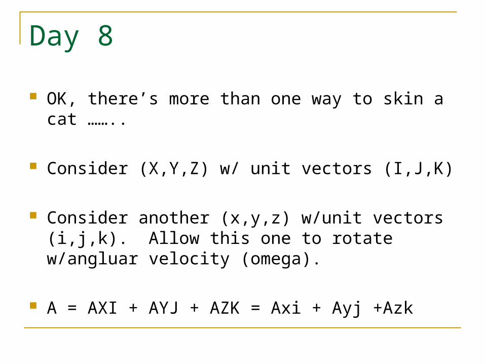
OK, there’s more than one way to skin a cat ……..

Consider (X,Y,Z) w/ unit vectors (I,J,K)

Consider another (x,y,z) w/unit vectors (i,j,k). Allow this one to rotate w/angluar velocity (omega).

A = AXI + AYJ + AZK = Axi + Ayj +Azk

Day 8

Now differentiate A w/r/t time (sytem 1 is const.! System 2 is rotating)

DA/dt = AX/dt I + dAY/dt J + dAZ/dt K = dAx/dt i + Ax di/dt + etc…..

i,j,k are unit vectors.

Di/dt = x i and dj/dt = x j and….

Day 8

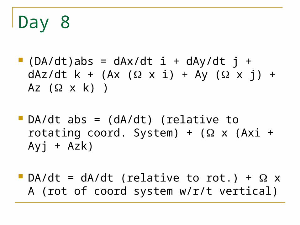
(DA/dt)abs = dAx/dt i + dAy/dt j + dAz/dt k + (Ax ( x i) + Ay ( x j) + Az ( x k) )

DA/dt abs = (dA/dt) (relative to rotating coord. System) + ( x (Axi + Ayj + Azk)

DA/dt = dA/dt (relative to rot.) + x A (rot of coord system w/r/t vertical)

Day 8/9

The rate of change of a vector in an absolute (inertial) frame of ref. Is equal to rate of chage observed in the rotating system + a term = to the cross product of the rotational vector and the arbitrary vector A!

Thus, you have just derived the expression for the coriolos force!

Day 9

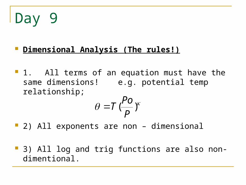
Dimensional Analysis (The rules!)

1. All terms of an equation must have the same dimensions! e.g. potential temp relationship;

2) All exponents are non – dimensional

3) All log and trig functions are also non-dimentional.

)(PPo

T

Day 9

4. The dimensions of differentials are the same as the dimensions of a differentiated quantity.

e.g., we can say d (ln (T))

Note: “specific” as a prefix implies the quantity is per unit mass and has the dimensions of (Q x M-

1) e.g., specific volume = vol / unit mass.

Day 9

Valid physical relationships must be dimensionally consistent with eachother, in other words X = Y must have the same units. Otherwise, we say X proportional to Y. Or X = AY where the units of AY are the same as X.

Caveat: Some proportionalities have consistent units.

Day 9

Non-dimensional analysis (Scale analysis)

(Mathematical formalization) Theoreticians like to look at equations in a non-dimensional sense, that is we choose characteristic time and space scales for some phenomena to be studied.

We essentially change coordinate systems:

(x,y) = L(x,y) where L is 2000 km t = Tt’ where T = 100000 sec (u,v) = U(u’,v’) U = 10 m/s

Day 9

In performing this type of analysis we can determine what processes are important for du/dt, for example, in the horizontal equation of motion on the desired scale (cyclone), we can perform this type of analysis for particular phenomena.

“Informal” Scale analysis

Similar to that of non-dimensionalization. Scale (size) analysis is also a powerful tool often used in meteorological derivations & the analysis of physical processes. This is a more “informal” method than non-dimensional analysis.

Day 9

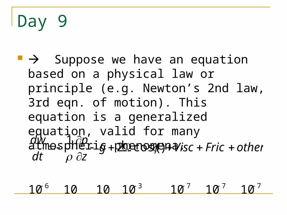
Suppose we have an equation based on a physical law or principle (e.g. Newton’s 2nd law, 3rd eqn. of motion). This equation is a generalized equation, valid for many atmospheric phenomena.

77736 10101010101010

)cos(21

otherFricViscgzp

dtdw

Day 9

We choose the scale we are interested in, the consider the order of magnitude, (e.g. the size and space scale) each term in the equation would have, for that particular scale of motion (again typical values, or estimates).

Then, we can neglect the smaller terms and simplify the equation. We’ll also know the error introduced in doing this (ratio of neglected to retained terms).

The equation is simplified, but now less general, it’s the trade-off for a simpler relationship.

Day 9

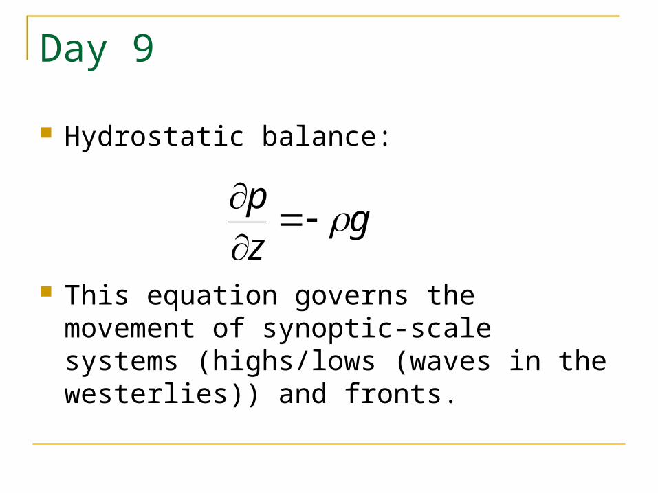
Hydrostatic balance:

This equation governs the movement of synoptic-scale systems (highs/lows (waves in the westerlies)) and fronts.

gzp

Day 9

Hydrostatic balance: the error

Error = Neglected Terms / Retained terms Error = 10-3 / 10 = 10-4 = 0.0001 = 0.01%

Thus this is a darned good estimate for synoptic and meso alpha scales.

Important Point! The equation is much simpler, but it’s only valid for these scales and has now lost its generality!

Day 9/10

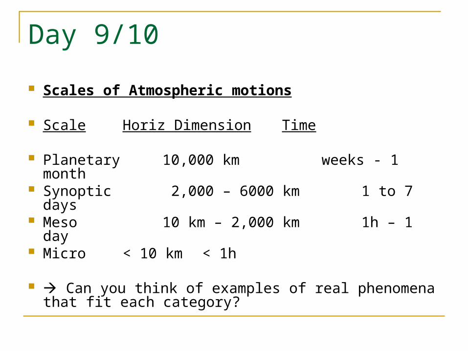
Scales of Atmospheric motions

Scale Horiz Dimension Time

Planetary 10,000 km weeks - 1 month Synoptic 2,000 – 6000 km 1 to 7 days Meso 10 km – 2,000 km 1h – 1

day Micro < 10 km < 1h

Can you think of examples of real phenomena that fit each category?

Day 10

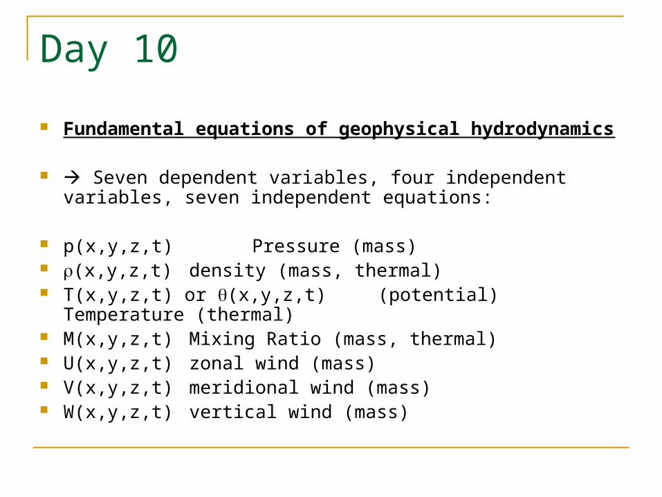
Fundamental equations of geophysical hydrodynamics

Seven dependent variables, four independent variables, seven independent equations:

p(x,y,z,t) Pressure (mass) (x,y,z,t) density (mass, thermal) T(x,y,z,t) or (x,y,z,t) (potential) Temperature (thermal) M(x,y,z,t) Mixing Ratio (mass, thermal) U(x,y,z,t) zonal wind (mass) V(x,y,z,t) meridional wind (mass) W(x,y,z,t) vertical wind (mass)

Day 10

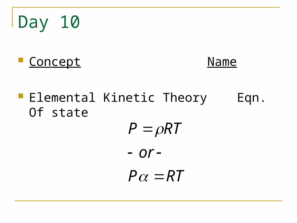
Concept Name

Elemental Kinetic Theory Eqn. Of state

RTP

or

RTP

Day 10

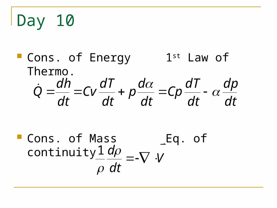
Cons. of Energy 1st Law of Thermo.

Cons. of Mass Eq. of continuity

dtdp

dtdT

Cpdtd

pdtdT

Cvdtdh

Q

Vdtd

1

Day 10

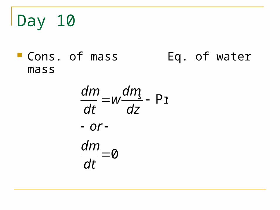
Cons. of mass Eq. of water mass

0

Pr

dtdm

ordzdm

wdtdm s

Day 10

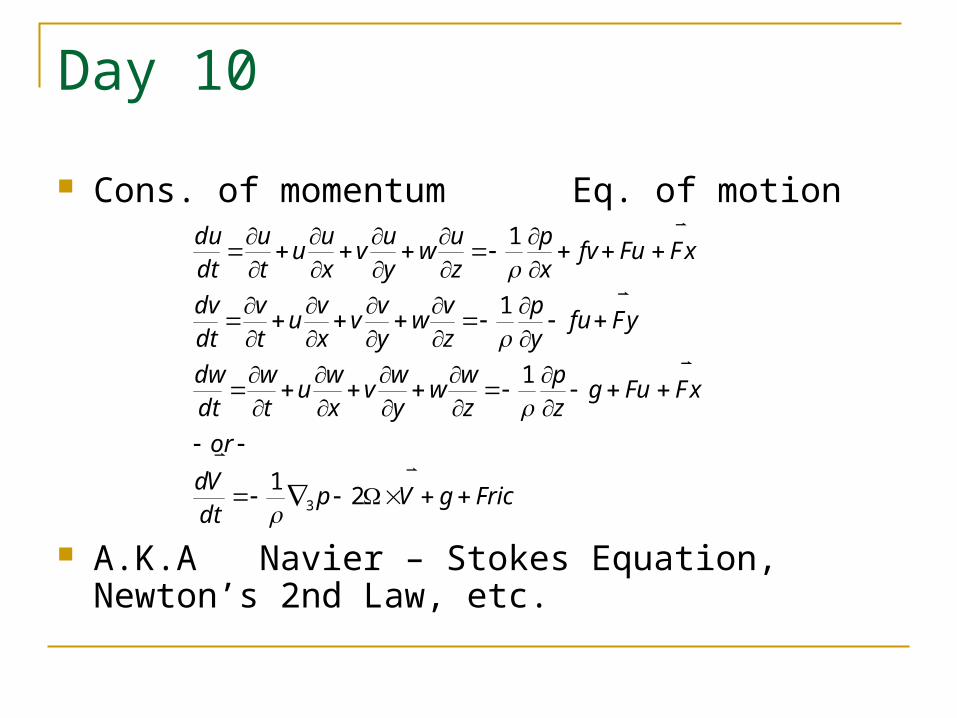
Cons. of momentum Eq. of motion

A.K.A Navier – Stokes Equation, Newton’s 2nd Law, etc.

FricgVpdtVd

or

xFFugzp

zw

wyw

vxw

utw

dtdw

yFfuyp

zv

wyv

vxv

utv

dtdv

xFFufvxp

zu

wyu

vxu

utu

dtdu

21

1

1

1

3

Day 10

Von Helmholtz 1858: In principle this is a mathematically solvable system (closed) given observed initial state and proper BC’s, the solution should yield all future states of the system.(The “rub” IC’s and BC’s).

Thus, forecasting is an initial value problem (Bjerknes, 1903)

These eqns. Are what will be studied in Atms 4310, 4320. These describe behavior of the atmosphere.

Solving these equations (Numerical methods and modeling classes – Atms 4800)

Day 10

The Thermodynamics of Dry Air (Holton Ch 2- 4)

Reminder: Dry air means DRY air (no moisture)!

Moist air: means water vapor present.

Dry air: (a homogeneous mixture of gasses from 0 – 80 km up – Homosphere)

Day 10/11

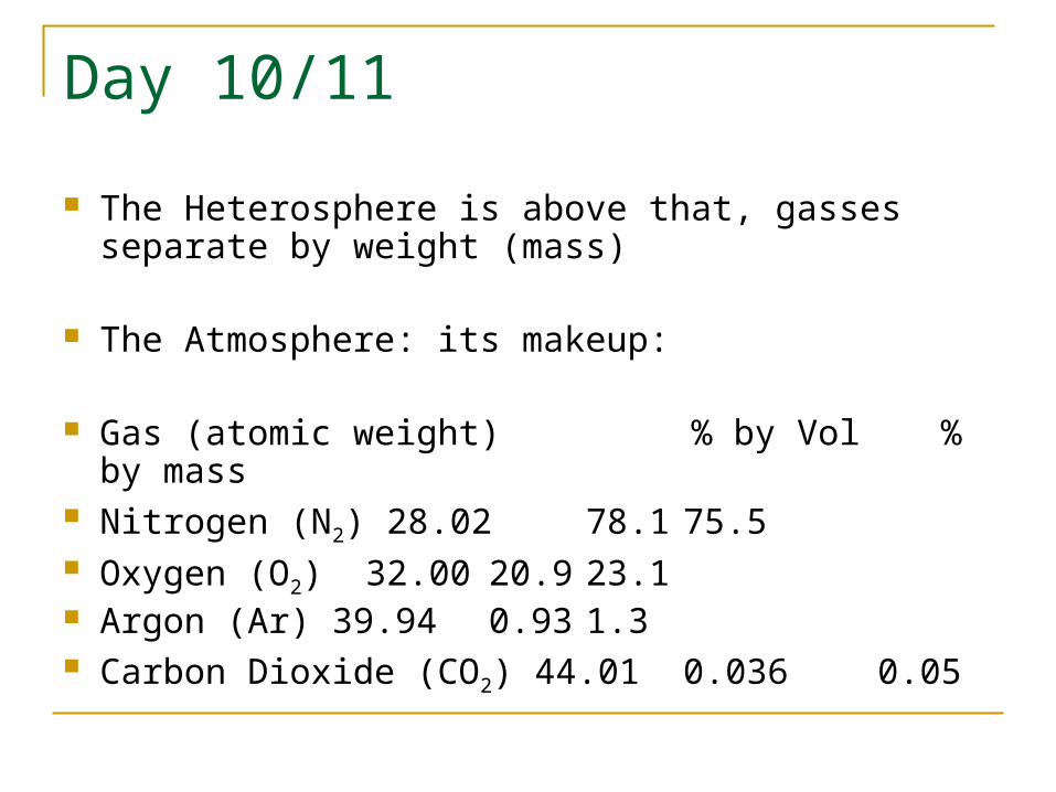
The Heterosphere is above that, gasses separate by weight (mass)

The Atmosphere: its makeup:

Gas (atomic weight) % by Vol % by mass Nitrogen (N2) 28.02 78.1 75.5 Oxygen (O2) 32.00 20.9 23.1 Argon (Ar) 39.94 0.93 1.3 Carbon Dioxide (CO2) 44.01 0.036 0.05

Day 10/11

Many other gases present in very small quantities (Ne, He, H, O3) they are called: Trace Gases

Thus if we calculate the atomic weight of air: 28.97 kg mol-1

Three of these are very important because despite the small quantities, they help determine the temperature structure of the troposphere and stratosphere: H2O, CO2, and O3

Day 11

H2O – is important within the hydrologic cycle, clouds, rain etc.. Water is the only substance in earth atmosphere that exists in all three phase at terrestrial pressures and temperatures.

Water Vapor and clouds are important in determining atmospheric structure due to their radiative properties (albedo, infrared).

Residence time 1 – 10 days.

Day 11

It is the most important and potent greenhouse gas, but its not homogeneously distributed!

CO2 – has homogeneous concentration. It is important because of it’s radiative properties in infrared. Its residence time near 100 years, thus important in longer term climate change. But, the CO2 cycle is not well known yet.

O3 – concentrated at 32km up (in stratosphere) due to solar and chemical reactions. It absorbs UV and emits infrared and responsible for the Stratosphere’s inversion.

Day 11

Near surface it is present in small amounts due to pollution, but it is highly poisonous.

Moist air

Water vapor extremely variable near 0 – near 4%

That’s 0 - 40 g/kg!

More typical: 1% 10 g/kg (Td = 57F)

Day 11

The variables of state

Mass (M) Density (mass/unit vol) () Specific volume (vol / unit mass)

Pressure: (Force/Area) is due to molecular collisions and the associated momentum changes independent of direction (a scalar). The force is normal to gas container walls. N m-2 = 1 Pa and 1mb = 102 Pa - or - kg m-1s-1

Day 11

Temperature: (T) a measure of the average internal energy of the molecules obtained during a state of equilibrium.

To read temperature there needs to be equilibrium established between the system and a temp sensor. Temp. determines direction of heat flow. (Kelvin, Celsius) 0o C = 273.15 K.

Ideal Gas: (Kinetic theory of gasses) is a collection of molecules that are

1) completely elastic spheres 2) with no attractive or repulsive forces, and 3) occupying no volume.

Day 11

Heat: is a form of energy, which can be transferred from a warmer to colder aubstance. Heat transfer by (really kinetic energy transfer):

Radiation Transfer of Electro- and Magnetic Conduction Transfer by molecular motions

(Contact) Convection Transfer by turbulent mixing (parcels,

bulk transport, advection) Latent (phase changes) "hidden heat"

Day 11

Relationships between our “state” variables, , , T, and P.

Boyle’s law:

Robert (Bob) Boyle (1600) said

if T is constant, then;

Day 11

P1 x V1 = P2 x V2 - or –

P x Volume = Constant

Recall, this is possible since Torricelli (1543)

invented the barometer!

So as a result of Boyle’s Law:

Day 11

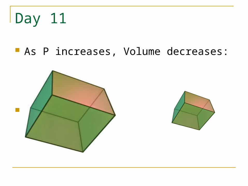
As P increases, Volume decreases:

Day 11

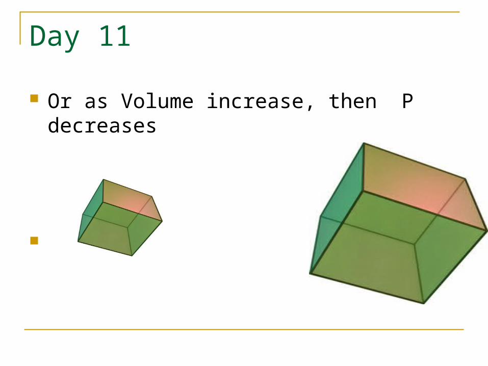
Or as Volume increase, then P decreases

Day 11

Charles’s Law:

Jaques Charles (1787) but stated formally J. Gay-Lussac (1802)

(1787 Bonus question: what else important happened in Sept. 1787?)

“Jack” said if pressure is kept constant then;

Volume1/Volume2 = Temperature1/Temperature2

Day 11

Or:

Volume/Temperature = Constant

Thus, when gas is heated, volume goes up, when gas is cooled, volume decreases!

Day 11/12

Combined or Ideal gas law

Constant = Pressure x Volume / Temperature

Derivation of Ideal Gas law for Atmosphere

Nee Avagadro’s hypothesis (derived experimentally, and derivable from kinetic theory of gasses)

Day 12

His hypothesis: Different gasses, each containing the same number of molecules, occupy the same volume at the same temperature and pressure.

Kilogram molecular weight: a kmol of material is it’s molecular weight expressed in kg. Thus, one kmol of water is 18.016 kg!

Number of molecules is Avagadro’s number (Av): 6.022x 1026

Day 12

Universal gas constant:

if we have a mixture of gases, each with it’s own ideal gas law (which is what Dalton’s Law implies!)

Po Volume(gas) = m(gas)R(gas)To where gas = 1,2,3, etc.

where m is the number of moles of each gas!

Day 12

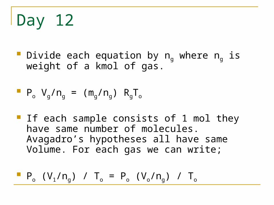
Divide each equation by ng where ng is weight of a kmol of gas.

Po Vg/ng = (mg/ng) RgTo

If each sample consists of 1 mol they have same number of molecules. Avagadro’s hypotheses all have same Volume. For each gas we can write;

Po (V1/ng) / To = Po (Vo/ng) / To

Day 12

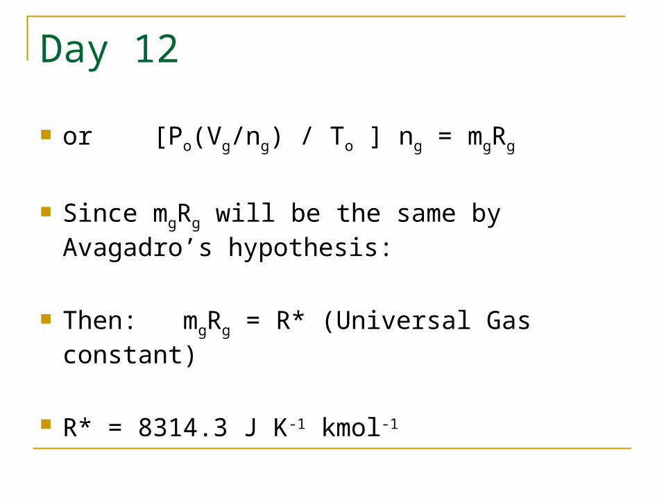
or [Po(Vg/ng) / To ] ng = mgRg

Since mgRg will be the same by Avagadro’s hypothesis:

Then: mgRg = R* (Universal Gas constant)

R* = 8314.3 J K-1 kmol-1

Day 12

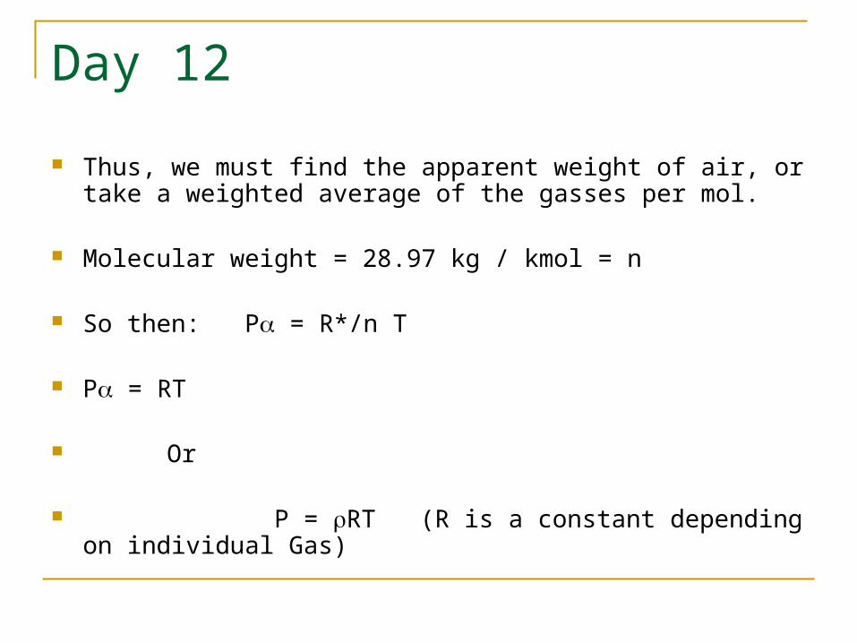
Thus, we must find the apparent weight of air, or take a weighted average of the gasses per mol.

Molecular weight = 28.97 kg / kmol = n

So then: P = R*/n T P = RT

Or P = RT (R is a constant depending on individual Gas)

Day 12

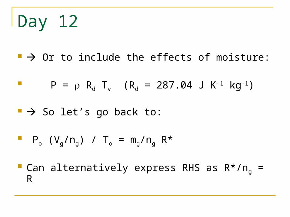
Or to include the effects of moisture:

P = Rd Tv (Rd = 287.04 J K-1 kg-1)

So let’s go back to:

Po (Vg/ng) / To = mg/ng R*

Can alternatively express RHS as R*/ng = R

Day 12

Thus in ideal gas law we must express as:

PV = R*/n (air) T where air = 28.97

V is volume, where Volume could be anything. Well we’ll specify some “specific volume”. ( = vol/unit mass) which equals 1 kg. This is still volume, we are not changing variables here or “playing fast and loose” with the math.

Thus:

P = R*/ (n air) T = RdT (- or - P = R*/n T = RdT)

Day 12

That’s for dry air. In accounting for moisture: ng = 18.016. The amount of water is very variable, and we could be specifying a different R for air every time amount of moisture changes.

That’s where concept of “virtual temperature” comes in. Thus,

P = Rd Tv -or- P = Rd Tv

Day 12

Q: Which is more dense, dry air or moist air?

Ever heard a baseball announcer talk about

the ball carrying on a warm humid night?

Dry air weights 28.97, throw in 18.016 for moist air.

Day 12

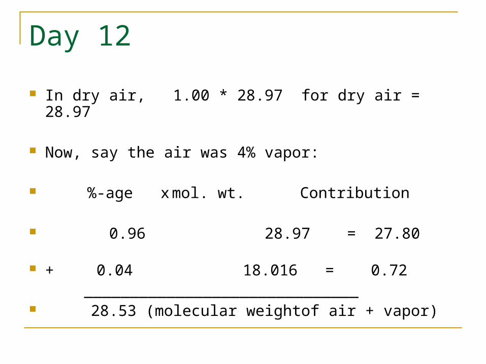
In dry air, 1.00 * 28.97 for dry air = 28.97

Now, say the air was 4% vapor:

%-age x mol. wt. Contribution

0.96 28.97 = 27.80 + 0.04 18.016 = 0.72 ______________________________ 28.53 (molecular weightof air + vapor)

Day 12/13

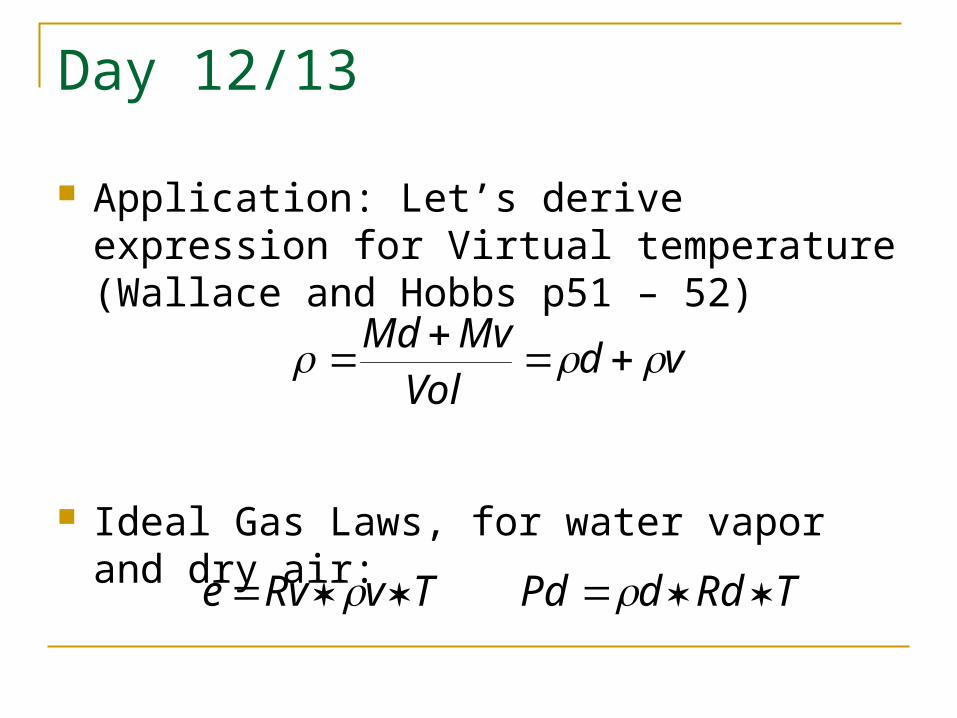
Application: Let’s derive expression for Virtual temperature (Wallace and Hobbs p51 – 52)

Ideal Gas Laws, for water vapor and dry air:

vdVol

MvMd

TRddPdTvRve

Day 13

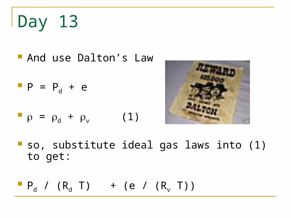
And use Dalton’s Law

P = Pd + e

= d + v (1)

so, substitute ideal gas laws into (1) to get:

Pd / (Rd T) + (e / (Rv T))

Day 13

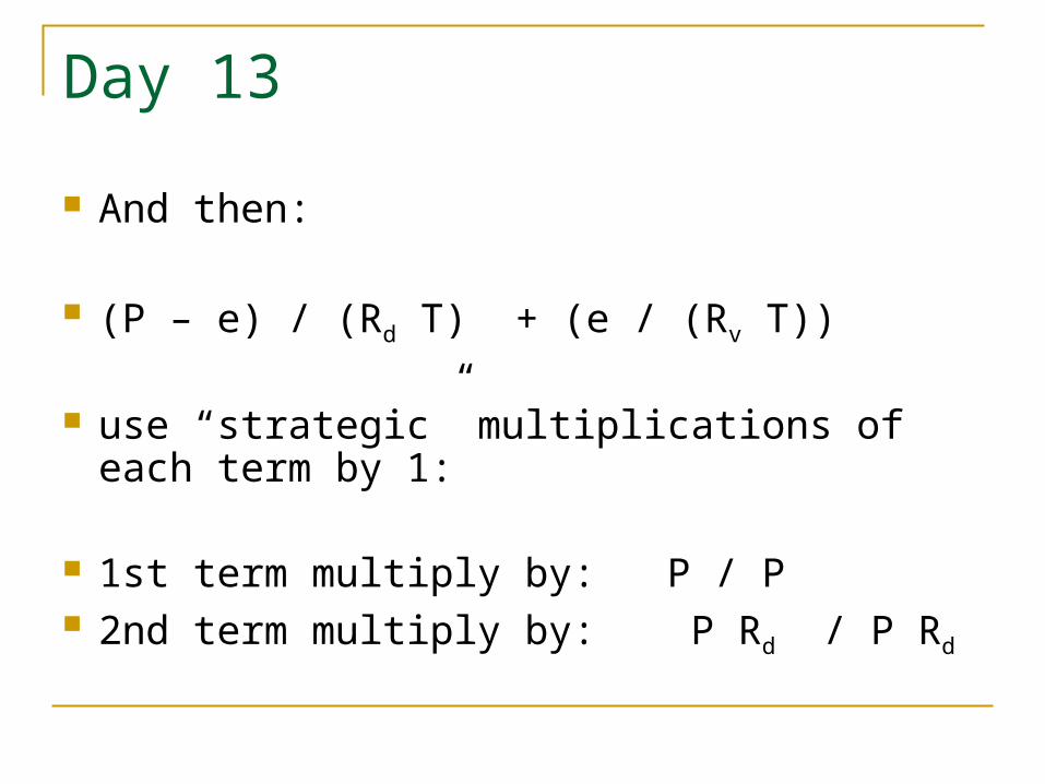
And then:

(P – e) / (Rd T) + (e / (Rv T))

use “strategic” multiplications of each term by 1:

1st term multiply by: P / P 2nd term multiply by: P Rd / P Rd

Day 13

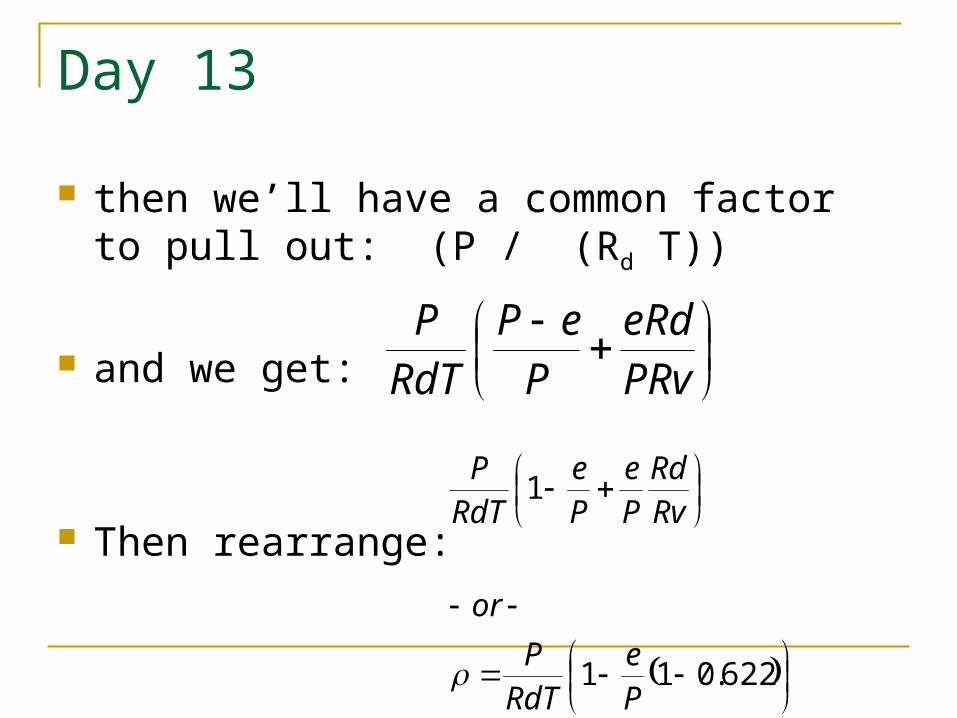
then we’ll have a common factor to pull out: (P / (Rd T))

and we get:

Then rearrange:

PRveRd

PeP

RdTP

622.011

1

Pe

RdTP

or

RvRd

Pe

Pe

RdTP

Day 13

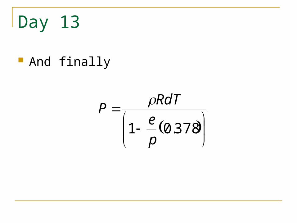
And finally

378.01pe

RdTP

Day 13

Celsius (1742) – Temperature scale (Centigrade)

Define: at P = Po = 1000 mb at a state of thermal equilibruim

Pure Ice and water mixture temp = 0o C

Pure water and steam mixture at equilibrium 100 o C

Day 13

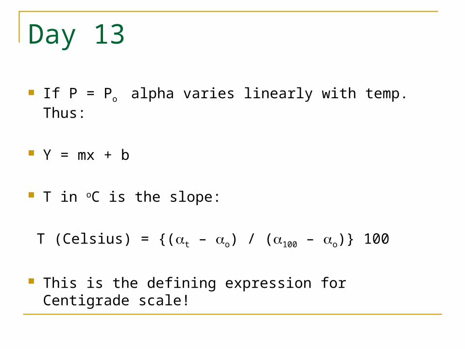
If P = Po alpha varies linearly with temp. Thus:

Y = mx + b

T in oC is the slope:

T (Celsius) = {(t – o) / (100 – o)} 100

This is the defining expression for Centigrade scale!

Day 13

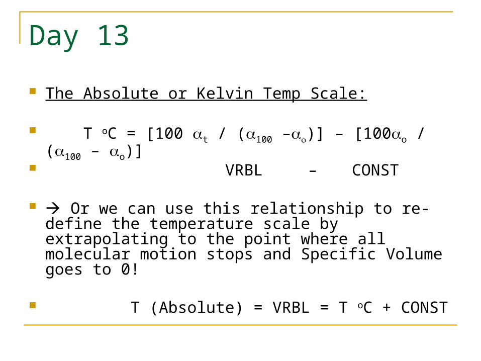
The Absolute or Kelvin Temp Scale:

T oC = [100 t / (100 –)] – [100o / (100 – o)] VRBL – CONST Or we can use this relationship to re-define the

temperature scale by extrapolating to the point where all molecular motion stops and Specific Volume goes to 0!

T (Absolute) = VRBL = T oC + CONST

Day 13

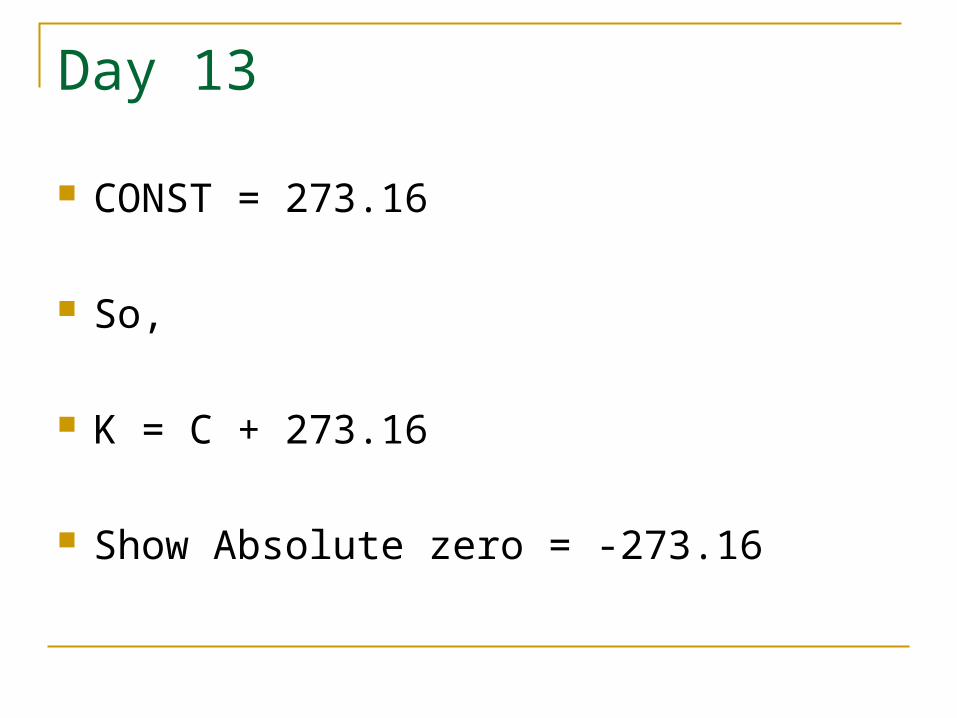
CONST = 273.16

So,

K = C + 273.16

Show Absolute zero = -273.16

Day 13

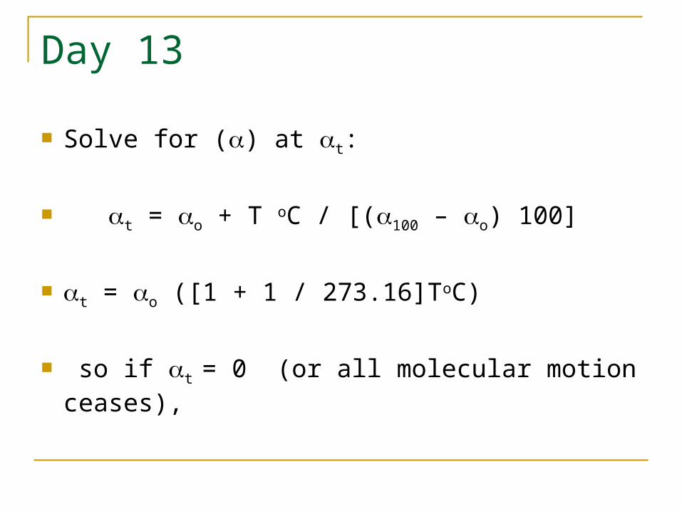
Solve for () at t:

t = o + T oC / [(100 – o) 100]

t = o ([1 + 1 / 273.16]ToC)

so if t = 0 (or all molecular motion ceases),

Day 13

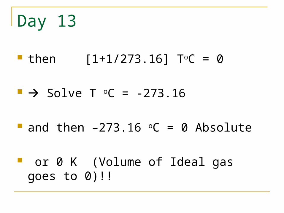
then [1+1/273.16] ToC = 0

Solve T oC = -273.16

and then –273.16 oC = 0 Absolute

or 0 K (Volume of Ideal gas goes to 0)!!

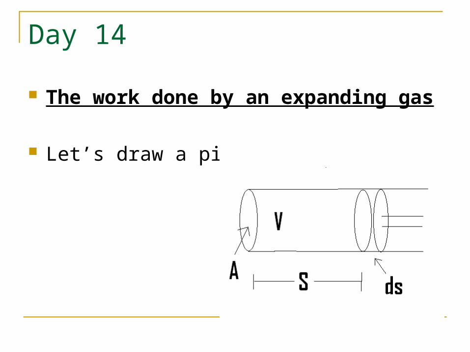
Day 14

The work done by an expanding gas

Let’s draw a piston:

Day 13

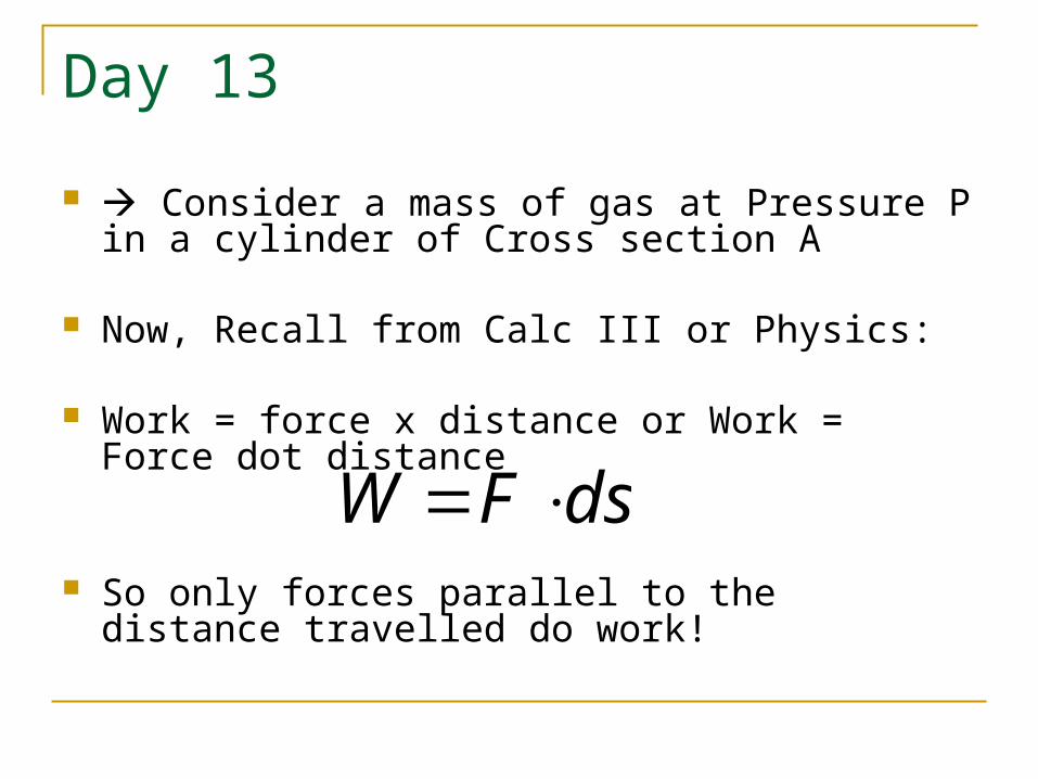
Consider a mass of gas at Pressure P in a cylinder of Cross section A

Now, Recall from Calc III or Physics:

Work = force x distance or Work = Force dot distance

So only forces parallel to the distance travelled do work!

dsFW

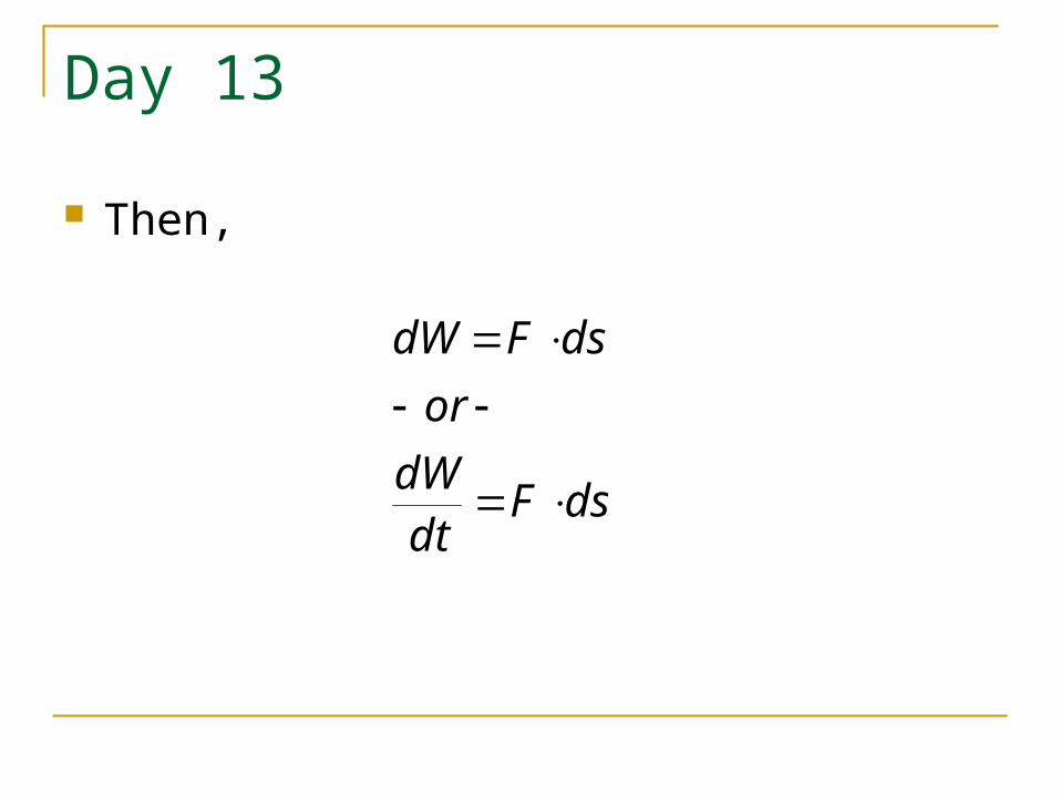
Day 13

Then,

dsFdtdW

or

dsFdW

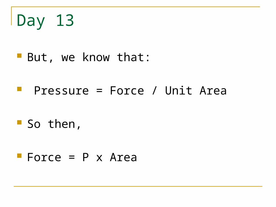
Day 13

But, we know that:

Pressure = Force / Unit Area

So then,

Force = P x Area

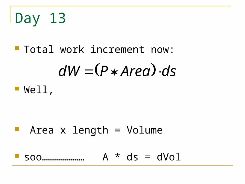
Day 13

Total work increment now:

Well,

Area x length = Volume

soo………………… A * ds = dVol

dsAreaPdW

Day 13

Then we get the result:

Work :

Let’s “work” with Work per unit mass:

Thus, we can start out with volume of only one 1 kg of gas!!!

PdVdW

mdV

PmdW

Day 13

Day 13

Day 13