Atmospheric correction of Earth-observation remote sensing ...

Atmospheric correction of Earth-observation remotesensing images by Monte Carlo method

Hanane Hadjit∗, Abdelaziz Oukebdane and Ahmad Hafid Belbachir

Laboratoire d’analyse et d’application du rayonnement (LAAR), Departement de physique,Universite des Sciences et de la Technologie d’Oran, B.P. 1505, El M’nouar, Oran, Algerie.

∗Corresponding author. e-mail: [email protected]

In earth observation, the atmospheric particles contaminate severely, through absorption and scatter-ing, the reflected electromagnetic signal from the earth surface. It will be greatly beneficial for landsurface characterization if we can remove these atmospheric effects from imagery and retrieve surfacereflectance that characterizes the surface properties with the purpose of atmospheric correction. Givingthe geometric parameters of the studied image and assessing the parameters describing the state of theatmosphere, it is possible to evaluate the atmospheric reflectance, and upward and downward trans-mittances which take part in the garbling data obtained from the image. To that end, an atmosphericcorrection algorithm for high spectral resolution data over land surfaces has been developed. It isdesigned to obtain the main atmospheric parameters needed in the image correction and the interpreta-tion of optical observations. It also estimates the optical characteristics of the Earth-observation imagery(LANDSAT and SPOT). The physics underlying the problem of solar radiation propagations that takesinto account multiple scattering and sphericity of the atmosphere has been treated using Monte Carlotechniques.

1. Introduction

Radiometers on satellites measure the radiancereflected by earth and atmosphere. The simple calib-ration of the sensor, in radiance or reflectance, doesnot provide information on surface that is directlyaccessible but a composite signal which dependson atmospheric conditions (gas absorption, moleculesand aerosols scattering) during measurements. Theneed of atmospheric correction is obvious. Thatis extracting, from the composite signal, infor-mation that depends only on the ground’s sur-face being studied. As atmospheric effects becomemore quantitative, the retrieval of accurate surfacereflectances becomes increasingly important. Forinstance, estimation of quantified surface properties

is based on surface reflectance. LANDSAT andSPOT satellites are invaluable resources for mon-itoring global change. Then, the atmospheric cor-rection is essential to adjust surface reflectance andcalculate ground properties.

There is a relatively long history of the quan-titative atmospheric correction of remote sensingimagery (Liang 2004). All methods reported inthe literature can be roughly classified in threedefinite groups (Bonn et al. 2001): the methodsbased on the invariants whose principle is to sup-pose the existence, in the study zone, of sur-faces which conserve their radiometric properties(deep water, roofs of buildings, etc.). Any changeobserved is, therefore, due to the atmospheric con-ditions. These methods require the identification of

Keywords. Atmospheric correction; reflectance; Monte Carlo method.

J. Earth Syst. Sci. 122, No. 5, October 2013, pp. 1219–1235c© Indian Academy of Sciences 1219

1220 Hanane Hadjit et al.

a dark object (lakes, shades, etc.) within the image,estimation of the signal level over that object, andsubtraction of that level from every pixel in theimage (Ahern et al. 1977; Chavez 1989). The mostused approaches are: Invariant-Object Method ofHall et al. (1991), Histogram Matching Method ofRichter (1996), Dark-Object Method developed byKaufman and Sendra (1988) and Contrast Reduc-tion Methods of Tanre et al. (1988). The majorweaknesses in this approach are in identifying asuitable object in a given scene, and once one islocated, is the assumption of zero reflectance forthat object (Teillet and Fedosejevs 1995). Also, theatmospheric correction can be conceded by simul-taneous ground measurements, which makes itpossible to find a direct relation between the digi-tal accounts and the pixel radiance. This methodis used in the update of satellite calibration curves.To allow a better statistical approach, this methodrequires a site where surface is most homogeneousand sufficiently large, which is not always obvious(Bonn et al. 2001).

A robust approach to the problem is to estimateatmospheric parameters of the image. The parame-ters can then be refined with any available ancillarymeasurements and iterative runs of an atmosphericmodelling program to achieve consistency betweenthe atmospheric parameters and the image data(Schowengerdt 2007). Estimation of atmosphericparameters from imagery itself is a difficult andchallenging step, since atmospheric effects includemolecular and aerosol scattering and absorptionby gases. Molecular scattering and absorption arerelatively easy to correct because of the stable con-centrations of these elements over both time andspace. The most difficult task is to estimate thespatial distributions of aerosols and water vapourdirectly from imagery (Liang 2004).

To retrieve surface reflectance, the effort must befocused on estimating the upward and downwardatmospheric path radiance. One begins by calcu-lating, from the image studied, the solar and obser-vation geometric parameters. Then an atmosphericmodel is specified, that is the pressure and tempe-rature profiles, and aerosol concentration and size.The calculation of extinction and scattering coeffi-cients of atmosphere constituents (aerosols andmolecules) is carried out. Then the probabilityof interaction for each constituent is determined.Once the geometrical and atmospheric parame-ters are calculated, the transport of the photonscan be simulated inside the atmosphere usingSART code (Spherical Atmosphere RadiationTransfer) (Hadjit 2007). Aerosols and moleculesphase functions govern the scattering interactionsbetween photons and atmospheric constituents.

The complexity and specificity of the problembeing solved, impose the use of techniques based

on analogue Monte Carlo. The path of a photon isconstructed as follows:

An emitted photon at the top of the atmosphereis followed until its extinction. Between these twoevents, a number of diffusions can happen. Scatter-ing changes the photon direction which is sampledfrom the phase functions. The history is terminatedwhen absorption takes place.

Satellite images of different regions were used toimplement the code SART which is designed toobtain the main atmospheric parameters needed inthe correction such as the atmospheric reflectance,and the upward and downward transmittances. Toconfirm SART results, a comparative study with 6Scode was performed separately for molecular andaerosol atmospheres for various geometrical andatmospheric conditions. In addition, a comparisonwas made between the measured reflectances andcalculated surface reflectances for different selectedareas. To complete this study an image of thedifference has been added for each study case inorder to show the effect of image correction.

2. Atmospheric model

The atmospheric model and the physics relatedto the effects of the atmosphere have been assem-bled and converted into a photon transport code,namely the SART code which can track each gene-rated photon. The use of Monte Carlo samplingtechniques allows the determination of a numberof parameters, mainly:

• The atmospheric reflectance, ρatm, which is ameasure of the parasite signal. It can be evalua-ted by counting the number of scattered photonsin the atmosphere;

• The downward transmittance, Ttot↓, that is thenumber of photons transmitted to the ground’ssurface;

• The upward transmittance, Ttot↑, that is thenumber of photons arriving at the ground’s sur-face and deflected towards the sensor.

It is clear that atmospheric effects are the result oftwo processes: absorption and scattering exerted,simultaneously, by the two major components ofthe atmosphere namely gases and aerosols.

Absorption by gas molecules or aerosols resultsin the disappearance of photons and corresponds tothe transformation of their energy into heat, hencea decrease in their number and a weakening of themeasured signal.

The model goes thorough two major steps: thegeometric and atmospheric parameter estimationand the surface reflectance retrieval.

Atmospheric correction of Earth-observation images 1221

2.1 Geometric and atmospheric parameters

The geometrical parameters introduced in the modelare calculated from data related to the remotesensing image being studied. The date, time ofacquisition, line and column numbers of the pixelin the image enable us to calculate the zenith andazimuth angles of observation, as well as the solarangles θs and ϕs (Vermote et al. 1997; Chami et al.2001; Capderou 2005).

In the solar spectrum (0.2–4 μm), the principalatmospheric gases responsible for absorption are:Oxygen (O2), Ozone (O3), water vapour (H2O) andCarbon dioxide (CO2). Absorption by aerosols ofanthropogenic origin, such as carbon soot, is higherthan the most aerosols of natural origin (liquids,dust) but is generally lower than absorption bygases.

Rayleigh scattering, which is specified by theRayleigh phase function, describes the scatteringby gas molecules whose dimensions are very smallcompared to the photon wavelength. However,scattering by aerosol particles whose sizes are com-parable to that of the wavelength is consideredto be anisotropic according to Mie theory. Theeffect of interacting particles or molecules is mea-sured by the attenuation (scattering or extinction)coefficients.

In our calculations, the extinction coefficientke(z) was approximated by a step function. Thetotal atmosphere layer of 100 km was divided into33 sublayers or spheres with different step sizes.Each layer is defined by its temperature, pressureand a model that defines aerosol types and concen-trations. SART use atmospheric data file represent-ing the pressure and the temperature as a functionof altitude for a standard atmosphere (USSTD76)(Thomas and Stamnes 1999).

Based on this, it is possible to calculate, for eachlayer, the corresponding attenuation coefficient asa function of the altitude z, given the attenua-tion coefficients of aerosols (katt, a) and molecules(katt, m)

katt (λ, z) = katt, a (λ, z) + katt, m (λ, z) . (1)

Aerosol attenuation coefficients depend on the pho-ton wavelength λ and altitude z, that is expressedby the following relation (Carr 2005):

katt, a (λ, z) = s (z) · katt, a (λ) (2)

katt, a(λ) is a scattering or extinction coefficientthat depends on the wavelength according to Mietheory (Kondratyev 1969; Shettle and Fenn 1979;Hinds 1998; Kokhanovsky 2008), s(z) is a scal-ing factor corresponding to extinction coefficientat λ = 550 nm and according to altitude: s(z) =k550(z) = s(0) · exp(−z/Ha) where Ha is aerosol

scaling factor (Ha = 2 km), and s(0) the extinctioncoefficient at surface related to the surface meteo-rological range V via the Koschmieder formula(Koschmieder 1924; Gueymard and Kambezidis1997; Carr 2005).

s (0) =3.916

V− 0.01159 (3)

V is defined as V = 1.306 VIS, where VIS is thevisibility given from the weather data.

Figure 1 shows the plots of aerosol extinction andscattering coefficients as a function of the wave-length, calculated by SART and 6S codes. Scatter-ing and extinction coefficients vary inversely withthe wavelength.

Figure 1. Extinction and scattering coefficients of aerosolsas a function of wavelength.

Figure 2. Scattering coefficient of molecules as a function ofaltitude.


Molecular scattering coefficient is approximatedby the following expression:

ks, m (z) = σs · Nr (z) · 105 (4)

σs is the scattering cross section (Rees 2001;Liou 2002) and Nr(z) the molecular concentration(cm−3) according to the pressure P , the tempera-ture T and the molecular density Ns(z = 0) =2.54143 1019 (Vermote et al. 1997).

Nr (z) = Ns

P (z)1013.25

273.15T (z)

.

Since the scattering coefficients of molecules varyinversely with the altitude and the wavelength,they are negligible for the upper layers of theatmosphere because of the low concentration ofatmospheric gases (figure 2).

However, the molecular extinction coefficientis calculated by taking into account the vertical

molecule distribution in the atmosphere (CESBIO2007).

ke, m (n) =τ0

Δh

[exp

(−hn+1

Hm

)− exp

(− hn

Hm

)]

(5)

hn and hn+1 are lower and upper heights of layern, Hm is the molecular scale factor (Hm = 8 km),Δh = hn+1 − hn and τ0 is the total optical thick-ness of the atmosphere calculated using the totaltransmittance Ttot.

The total transmittance, dependent on thecosine of the solar zenith angle, the wavelength andweather data during image acquisition (pressure,temperature and humidity), is calculated using themodified Meteorological Radiation Model (MRM)(Bird and Riordan 1986; Psiloglou et al. 2000;Badescu 2008) for the region of Oran (Es-Senia:35.38◦N, 0.36◦W, height = 90 m) and Mechria(34.49◦N, 0.62◦E, height = 1000 m) in Algeria,

Figure 3. Transmittance as a function of wavelength.


Quebec (53.67◦N, 66.86◦W, height = 600 m)in Canada and Railroad Valley Playa (38.50◦N,115.69◦W, height = 1435 m) in Nevada (USA).The total transmittance is defined as the productof Rayleigh transmittance.

Tr = exp{−mr / [λ4(115.6406 − 1.335 / λ2)]},

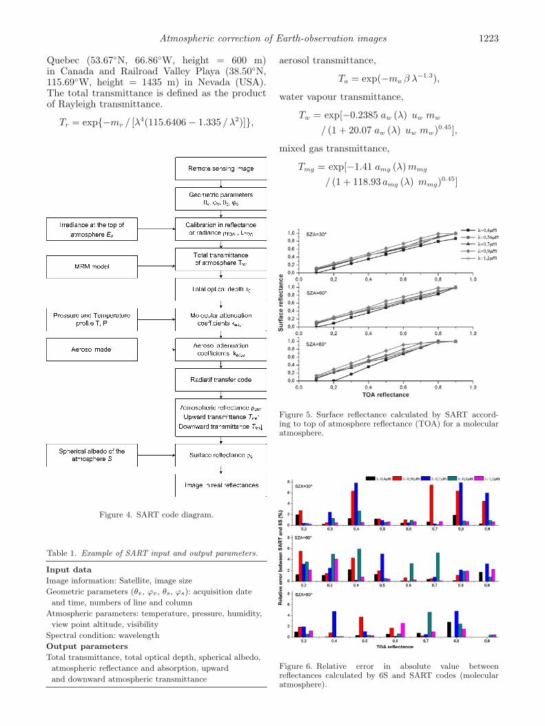
Figure 4. SART code diagram.

Table 1. Example of SART input and output parameters.

Input data

Image information: Satellite, image size

Geometric parameters (θv, ϕv, θs, ϕs): acquisition date

and time, numbers of line and column

Atmospheric parameters: temperature, pressure, humidity,

view point altitude, visibility

Spectral condition: wavelength

Output parameters

Total transmittance, total optical depth, spherical albedo,

atmospheric reflectance and absorption, upward

and downward atmospheric transmittance

aerosol transmittance,

Ta = exp(−ma β λ−1.3),

water vapour transmittance,

Tw = exp[−0.2385 aw (λ) uw mw

/ (1 + 20.07 aw (λ) uw mw)0.45],

mixed gas transmittance,

Tmg = exp[−1.41 amg (λ) mmg

/ (1 + 118.93 amg (λ) mmg)0.45]

Figure 5. Surface reflectance calculated by SART accord-ing to top of atmosphere reflectance (TOA) for a molecularatmosphere.

Figure 6. Relative error in absolute value betweenreflectances calculated by 6S and SART codes (molecularatmosphere).


and ozone transmittance,

To = exp (−ao (λ) uo mo) ,

where ma, mo and mw are the aerosol, the ozoneand the water vapour optical masses respectively(Gueymard and Kambezidis 1997), mr and mmg

are the pressure corrected airmasses of Rayleighand mixed gas (Iqbal 1983), uo and uw are,in that order, the ozone amount and the precip-itable water in vertical path (Leckner 1978; VanHeuklon 1979; Koussa et al. 2006; Badescu 2008),β is the Angstrom coefficient and ao, aw and amg

are the spectral absorption coefficients of ozone,water vapour and mixed gas (Gueymard 1995).

Figure 3 shows Rayleigh (Tr), Ozone (To), watervapour (Tw), gas mixture (Tmg), aerosol (Ta) andtotal (Ttot) transmittances calculated according tothe wavelength for Oran region. In the visible andnear-infrared, atmosphere is practically transpar-ent to electromagnetic radiation except for fewabsorption bands (1.2 and 2.7 μm) due to gas andwater vapour absorption.

The photon trajectory in atmosphere, which isa sequence of broken lines, can be specified bya series of three spatial coordinates (xi, yi, zi),i = 1, 2, . . ., n. These coordinates determine thesite of the ith interaction between photon andatmospheric constituents.

In order to calculate the free path length li, thatis the distance in km between two interaction sites,it might be convenient to use a dimensionless quan-tity, i.e., the optical depth τi which can be ran-domly sampled from an exponential distribution,then converted into a real distance using extinctioncoefficients (equation 6):

τi =

li∫0

ke (z) dz. (6)

Once τi is calculated, the layer index j is found byresolving the following double inequality:

n−1∑j=1

kej (li, j+1 − li, j) < τi <n∑

j=1

kej (li, j+1 − li, j) (7)

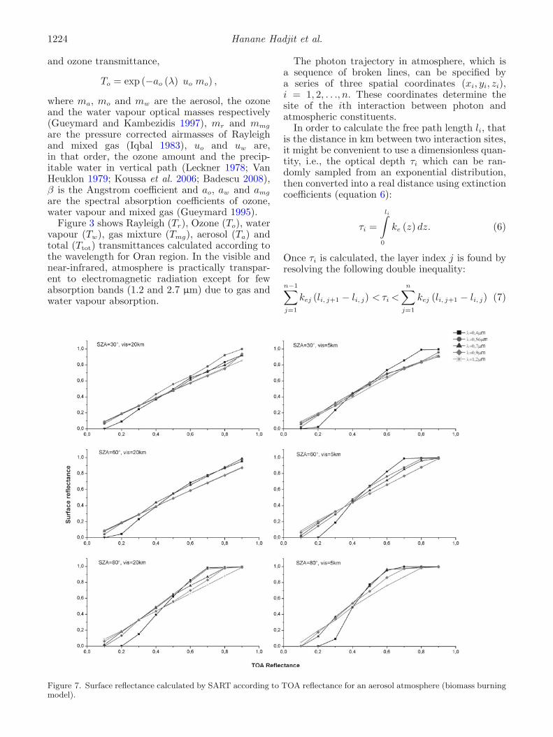
Figure 7. Surface reflectance calculated by SART according to TOA reflectance for an aerosol atmosphere (biomass burningmodel).


where li, j is the distance from the interaction site(xi, yi, zi) to the boundary of the spherical layerof index j, and kej is the total extinction coeffi-cient of layer j previously calculated. To find li,equation (7) can be reformulated as follows:

li = li, n +

[τi −

∑n−1

j=1 kj (li, j+1 − li, j)kn

]. (8)

In order to determine the type of interaction, arandom number is compared to the scatteringprobability ωp = ks/ke at point (xi, yi, zi) anda decision is taken regarding the realization ofa given interaction. In the same way, the scat-tering kind (by aerosols or molecules) is givenby using aerosol scattering probability defined asthe rapport between aerosol scattering and totalscattering coefficients.

After a scattering event, the new photon direc-tion is defined by the scattering angle θi and theazimuth angle ϕi. A set of two phase function isused, depending on the type of the particle involvedin the interaction. In the case of scattering byatmospheric molecules, the Rayleigh phase func-tion is used (Vermote et al. 1997).

P (θi) =34· 2 (1 − δ)

2 + δ

[1 + cos2 (θi)

](9)

where δ = 0.0279 is the depolarization factor whichtakes into account the anisotropy of molecularscattering.

In the case of scattering by aerosols, thephase function of Henyey–Greenstein is used todescribe the diffusion angle (Kokhanovsky 2008).However, the modified Henyey–Greenstein func-tion P (θi, a, g1, g2) is used in our code SART to

Figure 8. Relative error between reflectances calculated by 6S and SART codes for an aerosol atmosphere (biomass burningmodel).


model the maximum forward scatter and thelocal maximum backscatter (used also in DART)(Gascon 2001):

P (θi, a, g1, g2) =a (1 − g2

1)[1 + g2

1 − 2g1 cos (θi)]1,5

+(1 − a) (1 − g2

2)[1 + g2

2 − 2g2 cos (180 − θi)]1,5 .

(10)

The parameter a and the asymmetry factors g1 andg2 depend on the size distribution of aerosols andwavelength λ. In the current version of SART, theparameters a, g1 and g2 are constants whose numer-ical values are 0.95, 0.79 and 0.4, respectively. TheMonte Carlo techniques are used to sample θi andϕi. The scattering angle θi is given by samplingeither the aerosol or molecule phase functions usinginversion numerical process. However, the rejectionmethod is used to calculate cos ϕi and sinϕi usinga uniform distribution on [0, 2π] (Marchuk andMikhailov 1980).

Thus, the new position of the interaction siteis deduced from the old position, the directionalangles and the free path li.

2.2 Surface reflectance determination

The signal arriving at the sensor (radiometricsignal) is more or less contaminated by a noisesignal which is partly due to the atmospheric scat-tering. As a result, the radiometric signal dependson the surface characteristics, the incident irra-diance and the atmospheric effects. The relationof Kaufman and Sendra (1988) and Fraser et al.(1992) expresses the measured radiance LTOA asa function of the surface reflectance ρs as well asother parameters:

LTOA =ρs Ttot ↓ Ttot ↑ E0

π (1 − Sρs)cos (θ) + Latm (11)

where Ttot↑: upward atmospheric transmittance;Ttot↓: downward atmospheric transmittance; Latm:atmospheric radiance; S: spherical albedo of the

Figure 9. Surface reflectance calculated by SART according to TOA reflectance for an aerosol atmosphere (urban model).


atmosphere; and E0: irradiance at the top ofatmosphere.

Radiances are transformed into reflectances ρ asfollows (Bonn et al. 2001):

ρ =πL

cos (θ)E0

(12)

Leading to:

ρs =ρTOA − ρatm

Ttot ↓ Ttot ↑ +S (ρTOA − ρatm)(13)

ρTOA being the reflectance measured at the sensorlevel, ρatm the atmospheric reflectance and ρs thesurface reflectance which is the parameter beingsought.

An adequate radiative transfer model is capableof determining not only atmospheric reflectancesbut also upward and downward transmittances.

3. Results and discussions

Once the input parameters (geometric and atmo-spheric) and the TOA (top of atmosphere) irra-diance calculated, preliminary calculations usingcalibration coefficients are carried out to deter-mine the TOA reflectance image in the form of amatrix of radiometric values (Chander et al. 2009).These calculations set the stage for numericalexperiments to be conducted using SART code.

A given simulation result is always in the evalua-tion of: (1) the atmospheric reflectance and absorp-tion, (2) the downward transmittance and (3) theupward transmittance.

According to equation (13), the atmosphericcorrection of an image consists of calculating thesurface reflectance, by eliminating the atmosphericreflectance. Figure 4 represents the tasks accom-plished at various stages of the simulation. Datasets related to the radiative code used in oursimulations are represented in table 1. To confirm

Figure 10. Relative error between reflectances calculated by 6S and SART codes for an aerosol atmosphere (urban model).


Figure 11. Surface reflectance calculated by SART according to TOA reflectance for a mixed atmosphere (US standard andurban model).

the results obtained by SART code, a comparisonwas carried out with 6S code. The official websiteof 6S code (http://6s.ltdri.org) yields, online, thecorrection coefficients converted into reflectances(Vermote et al. 1997).

The study was made for TOA reflectances vary-ing from 0.1 to 0.9 under various atmospheric andgeometrical conditions and for several monochro-matic wavelengths. The surface reflectances calcu-lated by SART and 6S codes are compared. Threecases are studied: the first exploit a molecularatmosphere for various solar angles. Figure 5 repre-sents the SART surface reflectances for a standardUS atmosphere for several wavelengths λ.

The graphs show that the surface reflectanceincreases linearly with TOA reflectance to reacha limit value of 1. Also, the surface reflectanceincreases, contrary to TOA reflectance, when thewavelength increases except for λ=1.2 μm because ofthe strong absorption by gases.

The relative error εr, expressed as a percent-age between SART and 6S codes is calculatedusing the following formula εr = (ρSART − ρ6S) ∗

100/ρSART. Figure 6 summarizes the resultsobtained.

The relative error, in absolute value, between 6Sand SART codes does not exceed values 7%, 6%and 5% for solar zenith angles θs = 30◦, 60◦ and80◦, respectively.

In the second case, the aerosol atmosphere is con-sidered, thus absorption by gases is ignored. Thestudy is realized for two models of aerosol: urbanand biomass burning and for two values of visibil-ity 5 and 20 km. The results obtained are presentedin figures 7–10.

For a biomass burning model (figure 7), therelation between surface and TOA reflectances isalmost linear. At λ = 1.2 and 0.9 μm, surface andTOA reflectances are practically identical (slope ofthe curves is almost equal to the unit) where thescattering influence of aerosol is generally small. Atλ = 0.56, 0.4 and 0.7 μm, the scattering influenceincreases. Moreover, the difference between sur-face and TOA reflectances changes the sign withthe increase of TOA reflectances. When solar zenithangle equal to 80◦, the Mie scattering intervenes

http://6s.ltdri.org


Figure 12. Relative error between reflectances calculated by 6S and SART codes for a mixed atmosphere (US standard andurban model).

by increasing the aerosol influence for λ = 0.9and 1.2 μm. Consequently, for all wavelengths, thedifferences between surface and TOA reflectancesincrease and change sign when TOA reflectancesincrease.

The relative error (figure 8), in absolute value,between 6S and SART codes reach 8% for the twovalues of the visibility (5 and 20 km) and for thetwo solar zenith angles 30◦ and 60◦. When θs = 80,the relative error does not exceed 6%.

When VIS = 20 km (figure 9), the aerosol influ-ence of the urban model is intensified for the visiblewavelengths (0.4, 0.56 and 0.7 μm). This intensityincreases with the solar zenith angle, so the sur-face reflectance converges rapidly as value 1. AtVIS = 5 km, the aerosol influence is even larger.The surface reflectance increases quickly with TOAreflectance for all studied wavelengths. This rise islarge as the wavelength is small and the solar zenithangle is large.

Figure 10 shows that the maximum value ofrelative error, in absolute value, is located between

Figure 13. Average relative error between reflectances cal-culated by 6S and SART codes (mol: molecular atmosphere,bio: biomass burning aerosol atmosphere, urb: urban aerosolmodel, mix: mixed atmosphere).


4% (for θs = 80◦ and VIS = 20 km) and 7% (forVIS = 5 km and θs = 30◦ and 80◦). The rela-tive error is minimal for surface reflectances closeto the value 1. The last case represents the studyperformed on a standard US atmosphere withurban aerosol for two values of visibility 5 and20 km. Figures 11 and 12 summarize the resultsobtained.

Figure 11 illustrates the aerosol influence obser-ved previously (figure 9). Moreover, the molecularabsorption effect contributes to reduce the surfacereflectance, except for the wavelength λ = 0.9 μmbecause the total transmittance is large. Thisreduction is perfectly apparent for λ = 1.2 μm.

The relative error (figure 12), in absolute value,is integrated between 6% and 7% for the solar

zenith angles θs = 30◦ and 60◦, and reach 5% forθs = 80◦. For large TOA reflectances, the surfacereflectance reach 1 and the relative error betweenSART and 6S codes is practically null.

Figure 13 summarizes the average relativeerror, calculated over the studied wavelengths andsolar zenith angles, for the four models definedpreviously.

The average relative error, between SART and6S codes, is larger for an aerosol atmosphere thanmolecular and mixed atmospheres. Moreover, whenVIS = 20 km, the error is larger for biomass aerosolmodel than urban model. Whereas, for VIS = 5 kmthe contrary is observed. In general, the averagerelative error is lower for VIS = 5 km compared tothat for VIS = 20 km.

Table 2. Acquisition dates and weather data of studied images.

Acquisition Temperature Pressure Humidity Visibility

Image Satellite date (◦C) (mb) (%) (km)

1 LANDSAT-5(TM) 13/02/2011 10.6 1017.7 67 9.2

2 LANDSAT-5(TM) 01/06/1999 12.7 1010.3 34 16.1

3 LANDSAT-7(ETM+) 03/04/2011 22.4 1020.0 26 14

4 SPOT 4 06/09/2009 12.6 1029.5 57 15.0

Figure 14. LANDSAT-5 (TM) image (left) before and (centre) after correction and image of the difference (right) (north-west of Algeria, February 13, 2011 at 10:28 h).

Figure 15. LANDSAT-5 (TM) image (left) before and (centre) after correction and image of the difference (right) (RailroadValley Playa, Nevada USA, June 6, 1999 at 17:59).


The difference between SART and 6S codesis more reduced for molecular and mixed atmo-spheres than aerosol atmosphere. This difference isprimarily due to the used method (Monte Carlo forSART and successive orders of scattering for 6S).Nevertheless, both codes use the same equationsfor molecular absorption and scattering process-ing, which reduces the difference between the twocodes. Contrary, the modelling of aerosol scatteringin SART, based on the Henyey–Greenstein phasefunction and the Mie theory, differs from that usedin 6S where the aerosol optical thickness is calcu-lated beforehand. Consequently, the difference ismore significant.

SART code was used to calculate the surfacereflectance of several areas using some acquiredimages LANDSAT and SPOT on various dates.Table 2 presents acquisition dates and weatherdata of studied images.

The first studied site is the great sabkha ofOran in north Algeria. LANDSAT-5 (TM) image,that covers this region, is used. Raw and correctedimages and image of the difference are shown infigure 14.

The great sabkha of Oran, similar to an extendedlens with approximately 45 km of length and amaximum width of 12 km, is located at 15 km of

Oran town (3532′N, 0048′E) between two moun-tains: Murdjadjo in the north and Tessala in thesouth. It is a closed depression with a surface of568.70 km2. It is formed by a thin water layerwhose level varies according to seasons. However,the water of the sabkha is salted because it is fedby the streams of the watershed.

Railroad Valley Playa is a dry lake with a com-position dominated by clay. It is a desert sitewith no vegetation and aerosol loading is typicallylow. The overall size of the Playa is approximately15 km and it is located in central Nevada (38.504′N,115.692′W) between the towns of Ely and Tonopah.Result images are shown in figure 15.

There are many basins of internal drainage,known as Chotts, which fill with water during win-ter, but dry out and become salt pans in the sum-mer. The largest of these Chotts in Algeria is theChergui Chott. It is a closed depression of 8555 km2

of surface located in the western north of Algeria(34.49′N, 0.62′E) and containing permanent andseasonal saline, brackish, and freshwater lakes andpools, as well as hot springs.

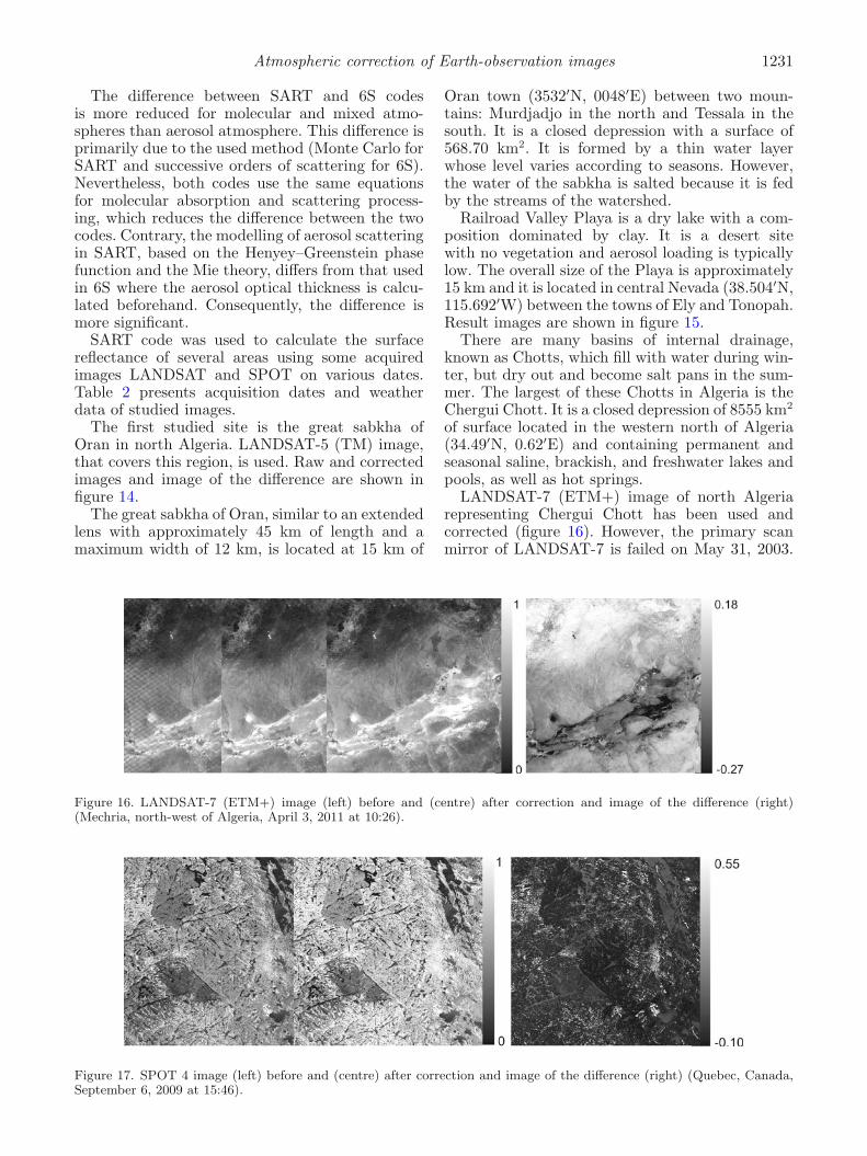
LANDSAT-7 (ETM+) image of north Algeriarepresenting Chergui Chott has been used andcorrected (figure 16). However, the primary scanmirror of LANDSAT-7 is failed on May 31, 2003.

Figure 16. LANDSAT-7 (ETM+) image (left) before and (centre) after correction and image of the difference (right)(Mechria, north-west of Algeria, April 3, 2011 at 10:26).

Figure 17. SPOT 4 image (left) before and (centre) after correction and image of the difference (right) (Quebec, Canada,September 6, 2009 at 15:46).


Thus, we correct the undersampling of scene beforeatmospheric correction (figure 16).

Also, the raw and corrected SPOT images ofQuebec region in Canada are given in figure 17.

The images of the difference (figures 14–17)illustrate the dissimilarity between the raw andcorrected images. Although the atmospheric con-ditions, and consequently atmospheric reflectanceand absorption, are the same ones for all scene, thecorrection is different because the surfaces, whichconstitute the scene, are variable. Thus, surfaceswith high albedo values (playa, city, etc.) appeardarker in the image of the difference than sur-faces with low albedo values (sea, vegetation, etc.).The atmospheric correction improves image con-trast. Thus, the dark pixels are darker and the

Figure 18. Reflectance of several areas as function asspectral band (great sabkha of Oran).

Figure 19. Reflectance of several areas as function asspectral band (Railroad Valley Playa).

correction, in this case, is negative (clear zones inthe image of difference), and the clear pixels areclearer and the correction is positive (dark zones inthe image of the difference). The atmosphere tendsto raise the signal resulting from dark surfaces anddecrease the signal resulting from clear surfaces.Radiometric values (reflectances) for selected areasrepresenting the sea and the ground from raw andcorrected images are shown in figures 18–21 for thevisible and near-infrared (NIR) bands.

Each zone (figure 18) is characterized by its ownsignature: the vegetation has a low reflectance inthe red and blue bands, a slightly larger reflectance

Figure 20. Reflectance of several areas as function asspectral band (Chergui Chott).

Figure 21. Reflectance of several areas as function asspectral band (Quebec).


in the green band and a strong reflectance in thenear-infrared band. The sea is characterized by ahigher reflectance in blue than in the red and thenear-infrared. The sabkha, in the dry zone, hasa reflectance which grows slightly with the wave-length because this soil is formed by clay and sandmixture with salt deposits due to the draining ofthe sabkha salted water. However, the water zoneis characterized by a weak reflectance reduction inthe red band and a very low reflectance in the nearinfra-red.

The ground of playa (figure 19) is character-ized by a slight increase of the reflectance withthe wavelength. It is spatially homogeneous witha composition consisting of compacted clay-richlacustrine deposits forming a relatively smooth sur-face. However, the surface suffer from the presenceof iron absorption (Fe3+) in the visible part of

the spectrum, characteristic of playas in this region(Chander 2009).

The following table (table 3) illustrates a com-parison between the results obtained by SART andthose measured by Thome for the acquired image ofthe Railroad Valley Playa on June 1, 1999 (Thome2001).

The relative error, in absolute value, variesbetween 0.04% and 5.43%.

The chott reflectance (figure 20) is comparableto that of the sabkha and playa. It increases with thewavelength in the dry area and decreases whenthe wavelength increases in the water area.

The SPOT image consists of several differentzones. The snow zone is characterized by a strongreflectance in the first three bands of the SPOTsatellite. The vegetation reflectance is high in thegreen and near-infrared bands and decreases in the

Table 3. A comparison with reflectances calculated by SART and Thome.

Band 1 Band 2 Band 3 Band 4

SART reflectance 0.6754 0.3397 0.3651 0.3939

Surface reflectance 0.253 0.332 0.365 0.393

Relative error (%) 5.4375 2.2828 0.0399 0.25

Figure 22. Histograms of image 1 (band 1, 2, 3 and 4).


red band. The black zones of the image representthe rivers characterized by a decreasing reflectancewith the wavelength (figure 21). Finally, for exam-ple and to visualize the differences between raw andcorrected images, histograms for different bands ofLANDSAT-5 image of Oran region were plotted infigure 22.

After correction, the histograms of the fourbands become more extended, which means thatthe images are contrasted. The blue band his-togram (B1) is composed of a large peak in theinterval [0.05, 0.1] which represents the vegetationand the sea and a second smaller peak representingthe salt lake of Oran.

On the other hand, the histograms of the greenand red bands (B2 and B3) are tri-modal. Theradiometric distribution of the values representsthree spaced population: sea, characterized bypeaks of values 0.05 in the green and 0.02 inthe red, the vegetation represented by the interval[0.1, 0.2] in the green band and [0.05, 0.25] in thered band and the salt lake and its environs whosereflectance exceeds value 0.25 in the green and redbands.

The histogram of the near-infrared band (B4)is bimodal, the two modes, representing the seaand the vegetation, are perfectly distinct. The saltlake is represented by short frequencies correspond-ing to the pixel numbers whose reflectances varybetween 0.05 and 0.25.

4. Conclusion

In this study, a new atmospheric correction code forremote sensing images has been developed, wherea radiative transfer model adapted for the spheri-cal atmosphere has been implemented and whosefundamental basis lies on the estimation of geomet-ric and atmospheric parameters namely the extinc-tion and scattering coefficients of aerosols andmolecules. The molecular coefficients are soughtonce the atmospheric temperature and pressureprofiles are defined. However, the aerosol coeffi-cients are obtained by resolving Mie equation. Thiswill set the stage for a comprehensive characteri-zation of the atmospheric state prior to the imageacquisition on one hand. On the other hand, thetracking of each generated photon is done by usingRayleigh and Henyey–Greenstein phase functionsto sample scattering angles, besides that, use ismade of extinction coefficients to determine sim-ple diffusion albedo and scattering probability foraerosols. SART uses simplest algorithms of theMonte Carlo method (rejection method, numericalinversion, discrete variables generation) based onthe random sampling, which is an advantage whenwe do not have much information of the studied

medium. Thus, for the atmosphere, the MonteCarlo method makes it possible to simulate, arbi-trarily, the optical thickness (representing absorp-tion and scattering) for each photon between twointeractions that allows to treat simultaneouslythe absorption and scattering processes. Moreover,Monte Carlo method permits to simulate photoninteraction with the atmosphere components and,as a result, to build a trajectory for each pho-ton (downward and upward ways) in an accept-able computing time (18 s for 1,000,000 of photonsgenerated for all the studied scene).

A comparative study related to the surfacereflectance was conducted using SART and 6Scodes, where a slight discrepancy was observedfor the three studied cases. This difference can beexplained by the fact that different methods arebeing used by the two codes, namely Monte Carlofor SART code and successive orders of scatter-ing for the 6S code. Moreover, the methods usedto calculate the input parameters (geometric andatmospheric) are different too.

To put to test this model, the atmosphericcorrection SART code was used to implementfour images of three satellites: LANDSAT-5,LANDSAT-7 and SPOT. Images of the differenceshow a significant change even though it is not visi-ble at first glance. These changes were confirmed byraw and corrected reflectance curves for differentsites in each image.

As a final remark we can say that this studywas, as a final remark, limited to the atmosphericeffect on remote sensing images and will be comple-mented by a study that takes into account groundand environment effects leading to a realistic imagecorrection.

References

Ahern F J, Goodenough D G, Jain S C, Rao V R andRochon G 1977 Use of clear lakes as standard reflec-tors for atmospheric measurements; In: Eleventh Inter-national Symposium on Remote Sensing of Environment,Ann Arbor, MI: Environmental Research Institute ofMichigan, pp. 583–594.

Badescu V (ed.) 2008 Modeling solar radiation at the Earth’ssurface: Recent advances (Berlin, Heidelberg: Springer-Verlag), 537p.

Bird R E and Riordan C 1986 Simple solar spectral modelfor direct and diffuse irradiance on horizontal and tiltedplanes at the earth’s surface for cloudless atmospheres;J. Climate Appl. Meteorol. 25 87–97.

Bonn F J, Collet C, Caloz R and et Rochon G 2001Precis de teledetection: Traitements numeriques d’imagesde teledetection; Association des universites partielle-ment ou entierement de langue francaise, UREF, Agenceuniversitaire de la francophonie, PUQ, 160p.

Capderou M 2005 Satellites: Orbits and Missions (France:Springer-Verlag), 544p.

Carr S B 2005 The aerosol models in MODTRAN: Incor-porating selected measurements from northern Australia,


Intelligence, Surveillance and Reconnaissance Division,Defence Science and Technology Organisation, DSTO-TR-1803, 67p.

Centre d’Etudes Spatiales de la BIOsphere (CESBIO) 2007Principes Physique de DART, reference DART Hand-book, Associated Industrial Company: Magellium, 70p.

Chami M, Santer R and Dilligeard E 2001 Radiative transfermodel for the computation of radiance and polarization inan ocean–atmosphere system: Polarization properties ofsuspended matter for remote sensing; Appl. Opt. 40(15)2398–2416.

Chander G 2009 Questionnaire for information regarding theCEOS WGCV IVOS subgroup Cal/Val test sites for landimager radiometric gain, Version 1.1, CEOS, 25p.

Chander G, Markham B L and Helder D L 2009 Summaryof current radiometric calibration coefficients for LandsatMSS, TM, ETM+, and EO-1 ALI sensors; Remote Sens.Environ. 113 893–903.

Chavez P S Jr 1989 Radiometric calibration of LandsatThematic Mapper multispectral images; Photogram. Eng.Rem. Sens. 55(9) 1285–1294.

Fraser R S, Ferrare R A, Kaufman Y J, Markham B L andMattoo S 1992 Algorithm for atmospheric corrections ofaircraft and satellite imagery; Int. J. Remote Sens. 13(3)541–557.

Gascon F 2001 Modelisation Physique d’Images deTeledetection Optique; These de doctorat, universite deToulouse III, discipline: signaux, images et acoustique,174p.

Gueymard C 1995 SMARTS2, Simple Model of the Atmo-spheric Radiative Transfer of Sunshine: Algorithms andPerformance Assessment; Rep. FSEC-PF-270–95, FloridaSolar Energy Center, Cocoa, FL, 84p.

Gueymard C A and Kambezidis H D 1997 Solar radiationand daylight models; In: Solar Spectral Radiation, Else-vier Butterworth-Heinemann, Linacre House, Jordan Hill,Oxford OX2 8DP, pp. 221–301.

Hadjit H 2007 Resolution par la Methode Monte Carlo desProblemes de Transfert Radiatif dans une AtmosphereSpherique, these de Magister, universite de science et dela technologie d’Oran, 127p.

Hall F G, Strebel D E, Nickeson J E and Goetz S J 1991Radiometric rectification: Toward a common radiometricresponse among multidate, multisensor images; RemoteSens. Environ. 35 11–27.

Hinds W C 1998 Aerosol technology: Properties, behavior,and measurement of airborne particles, 2nd edn, A Wiley-Interscience Publication, John Wiley & Sons, INC., 200p.

Iqbal M 1983 An introduction to solar radiation; AcademicPress, Toronto.

Kaufman J Y and Sendra C 1988 Algorithm for automaticatmospheric corrections to visible and near-IR satelliteimagery; Int. J. Remote Sens. 9(8) 1357–1381.

Kokhanovsky A A 2008 Aerosol optics: Light absorption andscattering by particles in the atmosphere; Springer–Praxisbooks in Environmental Sciences, 154p.

Kondratyev K Y A 1969 Radiation in the atmosphere,Volume 12, Academic Press, INC, 929p.

Koschmieder H 1924 Theorie der horizontalen Sichtweite;Beitr. Phys. Atmos. 12 33–53.

Koussa M, Malek A and Haddadi M 2006 Validation dequelques modeles de reconstitution des eclairements dusau rayonnement solaire direct, diffus et global par cielclair; Revue des Energies Renouvelables 9N◦4 307–332.

Leckner B 1978 The spectral distribution of solar radiationat the earth’s surface – elements of a model; Solar Energy20 143–150.

Liang S 2004 Quantitative remote sensing of land surfaces,John Wiley & Sons, Inc., 562p.

Liou K N 2002 An introduction to atmospheric radia-tion, 2nd edn, Academic Press, An imprint of ElsevierScience, 599p.

Marchuk G I and Mikhailov G A 1980 The Monte Carlomethods in atmospheric optics; Springer series in opticalsciences, 210p.

Psiloglou B E, Santamouris M and Asimakopoulos D N 2000Atmospheric broadband model for computation of solarradiation at the earth’s surface: Application to mediter-ranean climate, Birkhauser Verlag, Basel; Pure Appl.Geophys. 157 829–860.

Rees W G 2001 Physical principles of remote sensing ; 2ndedn, Cambridge University Press, 369p.

Richter R 1996 A spatially adaptive fast atmospheric cor-rection algorithm; Int. J. Remote Sens. 17 1201–1214.

Schowengerdt R A 2007 Remote sensing: Models and meth-ods for image processing, 3rd edn, Academic Press, Animprint of Elsevier Science, 558p.

Shettle E P and Fenn R W 1979 Models for the Aerosols ofthe lower atmosphere and the effects of humidity on theiroptical properties, Optical Physics Division, Project 7670,Air Force Geophysics Laboratory, Air Force SystemsCommand, Usaf, 94p.

Tanre D, Deschamps P Y, Devaux C and Herman M 1988Estimation of Saharan aerosol optical thickness from blur-ring effects in Thematic Mapper data; J. Geophys. Res.93 15,955–15,964.

Teillet P M and Fedosejevs G 1995 On the dark targetapproach to atmospheric correction of remotely senseddata; Canadian J. Remote Sens. 21(4) 374–387.

Thomas G E and Stamnes K 1999 Radiative Transfer inthe Atmosphere and Ocean, Cambridge Atmospheric andSpace Science Series, Cambridge University Press, 540p.

Thome K J 2001 Absolute radiometric calibration of Land-sat 7 ETM+ using the reflectance-based method; RemoteSens. Environ. 78 27–38.

Van Heuklon T K 1979 Estimating atmospheric ozone forsolar radiation models; Solar Energy 22 63–68.

Vermote E, Tanre D, Deuze J L, Herman M andMorcrette J 1997 Second Simulation of the Satellite Signalin the Solar Spectrum (6S), 6S User Guide Version 2, For-merly affiliated to Laboratoire d’Optique Atmospherique,part 2, 83p.

MS received 18 June 2012; revised 25 February 2013; accepted 25 February 2013

Atmospheric correction of Earth-observation remote sensing ...

Documents

Transcript of Atmospheric correction of Earth-observation remote sensing ...