Atmospheric boundary layer characteristics from ceilometer measurements. Part 1: a new method to track mixed layer height and classify clouds Article 

Published Version 

Creative Commons: Attribution 4.0 (CC­BY) 

Open Access 

Kotthaus, S. and Grimmond, C. S. B. (2018) Atmospheric boundary layer characteristics from ceilometer measurements. Part 1: a new method to track mixed layer height and classify clouds. Quarterly Journal of the Royal Meteorological Society, 144 (714). pp. 1525­1538. ISSN 1477­870X doi: https://doi.org/10.1002/qj.3299 Available at http://centaur.reading.ac.uk/76370/ 

It is advisable to refer to the publisher’s version if you intend to cite from the work.  See Guidance on citing  .

To link to this article DOI: http://dx.doi.org/10.1002/qj.3299 

Publisher: Royal Meteorological Society 

All outputs in CentAUR are protected by Intellectual Property Rights law, including copyright law. Copyright and IPR is retained by the creators or other 

copyright holders. Terms and conditions for use of this material are defined in the End User Agreement  . 

www.reading.ac.uk/centaur   

CentAUR 

Central Archive at the University of Reading 

Reading’s research outputs online

Received: 15 November 2017 Revised: 15 March 2018 Accepted: 22 March 2018

DOI: 10.1002/qj.3299

R E S E A R C H A R T I C L E

Atmospheric boundary-layer characteristics from ceilometermeasurements. Part 1: A new method to track mixed layer heightand classify clouds

Simone Kotthaus1,2 C. Sue B. Grimmond1

1Department of Meteorology, University ofReading, Reading, UK2Institute Pierre Simon Laplace, Centre Nationalde la Recherche Scientifique, École Polytechnique,91128 Palaiseau, France

CorrespondenceSimone Kotthaus, Department of Meteorology,University of Reading, PO Box 217 Reading,RG6 6AH, UK.Email: s.kotthaus@reading.ac.uk

Funding informationEU FP7, BRIDGE. EU H2020, URABNFLUXES.NERC ClearfLo, NE/H003231/1. NERC APHHChina AirPro. Newton Fund/Met Office,CSSP-China. University of Reading. King’sCollege London.

The use of Automatic Lidars and Ceilometers (ALC) is increasingly extended beyondmonitoring cloud base height to the study of atmospheric boundary layer (ABL)dynamics. Therefore, long-term sensor network observations require robust algo-rithms to automatically detect the mixed layer height (ZML). Here, a novel automaticalgorithm CABAM (Characterising the Atmospheric Boundary layer based on ALCMeasurements) is presented. CABAM is the first non-proprietary mixed layer heightalgorithm specifically designed for the commonly deployed Vaisala CL31 ceilome-ter. The method tracks ZML, takes into account precipitation, classifies the ABLbased on cloud cover and cloud type, and determines the relation between ZML andcloud base height. CABAM relies solely on ALC measurements. Results performwell against independent reference (AMDAR: Aircraft Meteorological Data Relay)measurements and supervised ZML detection. AMDAR-derived temperature inver-sion heights allow ZML evaluation throughout the day. Very good agreement is foundin the afternoon when the mixed layer height extends over the full ABL. However,during night or the morning transition the temperature inversion is more likely asso-ciated with the top of the residual layer. From comparison with SYNOP reports, theABL classification scheme generally correctly distinguishes between convective andstratiform boundary-layer clouds, with slightly better performance during daytime.Applied to 6 years of ALC observations in central London, Kotthaus and Grimmond(2018), a companion paper, demonstrate CABAM results are valuable to characterisethe urban boundary layer over London, United Kingdom, where clouds of varioustypes are frequent.

KEYWORDS

ABL, ALC, AMDAR, boundary-layer clouds, CABAM, ceilometer, mixed layerheight

Abbreviations: ABL, atmospheric boundary layer; agl, above ground level; ALC, automatic lidars and ceilometers; AMDAR, Aircraft Meteorological Data Relay; AN, afternoon(mid-point between solar noon and sunset); B, end time of layer; CABAM, Characterising the Atmospheric Boundary layer based on ALC Measurements; CBH, cloud base height;CC, cloud cover; Cu, cumulus cloud, also ABL class of days dominated by Cu; d, prefix, indicating a difference; D, second derivative of attenuated backscatter; daySR, 24 hr periodscentred on sunrise; ET, evening transition; g, range gate index; G, vertical gradient of attenuated backscatter; Hday, duration of day; Hnight, duration of night; i, index of iteration; IQR,inter-quartile range; K, layer detection density; L, layer duration; MBE, mean bias error; MH±1, mixed layer height at end of previous day/beginning of next day; ML, mixed layer;MN, midnight; MT, morning transition; N, number of layers; n, number of layers fulfilling certain criteria; NT, nocturnal layer after sunset; P, number of points forming a layer; p,percentile; q, index of layer; r, range (distance from instrument); R, size of range window; RL, residual layer; RLH, height of residual layer; RMSE, root-mean-square error; SC,stratocumulus cloud, also ABL class of days dominated by Sc; SN, solar noon; SNR, signal-to-noise ratio; SR, sunrise; SS, sunset; St, stratus cloud, also ABL class of days dominatedby St; T, time window; t, time; tp, time step with precipitation detected; v, factor ; z, height above ground; zmax, maximum mixed layer height; zmin, minimum mixed layer height; ZML,mixed layer height; ztop, topmost layer by time step detected by CABAM algorithm; zΔT, height of temperature inversion; Δz, height difference; 𝜎, standard deviation; 𝜎*, standarddeviation after removal of temporal trend; 𝛽 , range-corrected attenuated backscatter, smoothed in range and time; 𝛽′, range-corrected attenuated backscatter.

This is an open access article under the terms of the Creative Commons Attribution License, which permits use, distribution and reproduction in any medium, provided the originalwork is properly cited.© 2018 The Authors. Quarterly Journal of the Royal Meteorological Society published by John Wiley & Sons Ltd on behalf of the Royal Meteorological Society.

Q J R Meteorol Soc. 2018;144:1525–1538. wileyonlinelibrary.com/journal/qj 1525

1526 KOTTHAUS AND GRIMMOND

1 INTRODUCTION

The mixed layer (ML) height (ZML) can be identified bydifferent physical indicators. The top of the atmosphericboundary layer (ABL) is usually marked by a clear temper-ature inversion, decrease in humidity and strong turbulence,so that the Richardson number is often used to detect thisheight based on radiosonde profiles (e.g. Piringer et al., 2007).The height of maximum turbulence can be determined fromDoppler lidar observations (e.g. Barlow et al., 2011) or SonicDetecting And Ranging (SODAR) systems (e.g. Emeis et al.,2008). However, the latter are restricted to shallow bound-ary layers due to their limited range. Automatic lidars andceilometers’ (ALC) compact design, low cost, and high rangeresolution (∼10 m) make them advantageous to many of thealternative systems.

ALC aerosol-studies have explored particles dispersedwithin the ABL (e.g. Tsaknakis et al., 2011) and layers fromSaharan dust (e.g. Knippertz and Stuut, 2014), biomass burn-ing (Mielonen et al., 2013), and volcanic ash (e.g. Wiegneret al., 2012; Marzano et al., 2014; Nemuc et al., 2014). Devel-oped as cloud base height (CBH) recorders, ALC provideautomatic CBH estimates, with multiple cloud layers iden-tified (Martucci et al., 2010). Given they are automatic andlow maintenance, ALC networks are widespread (e.g. DWD,2018).

To exploit ALC data for ABL metrics, automatic ZML

retrieval methods are required. Although considerable efforthas been made to improve various algorithms for the detec-tion of ZML from ALC attenuated backscatter profiles (section2.1), no open-source algorithm is available that utilises onlyALC observations to adequately and continuously detect ZML

patterns from Vaisala CL31 ceilometers. This commonlydeployed instrument has the advantage of reaching completeoptical overlap at low ranges so that the whole observedprofile is available for mixed layer height analysis.

Evaluation of ZML results is demanding, given referencemeasurements are often scarce and all observational meth-ods are challenged by the complex task of layer attribution(section 2.2). Radiosondes, commonly used as the reference,are often limited in temporal resolution. In regions with heav-ily trafficked air-space, Aircraft Meteorological Data Relay(AMDAR) observations provide an alternative. Still, carefulanalysis is needed when temperature inversions indicate thetop of the residual layer (RL) rather than the mixed layer.

While there is common agreement on the applicabilityof boundary-layer aerosols as a tracer for atmospheric mix-ing under cloud-free conditions (Barlow, 2014), the limitsof interpretation of attenuated backscatter profiles in cloudyand rainy conditions are yet to be determined. Caicedo et al.(2017) discuss the implications of ALC signal response inclouds for different ZML-methods. To address the role ofclouds in sufficient detail (Schween et al., 2014), classifica-tion of ABL by not only cloud cover but also cloud type isrequired (section 2.3).

Most studies exclude rainy periods based on nearby sur-face station measurements. However, these are likely to misscertain types of precipitation events, such as rainfall evapo-rating above ground level and light rainfall. de Bruine et al.(2017) explicitly show examples of ZML detected during rain-fall which highlight the risk for false layer attribution undercomplex conditions. For example, the evaporation layer cancause strong negative gradients in the attenuated backscatter(“dark band”) that might lead to false layer attribution.

The objective of this work is to describe and evaluate anovel algorithm for the characterisation of the ABL. TheCABAM (“Characterising the Atmospheric Boundary layerbased on ALC Measurements”) algorithm uses only ALCmeasurements to track ZML and to classify the ABL by cloudcover and cloud type (relating ZML to CBH), incorporating anovel rainfall filter. Specifically designed for use with VaisalaCL31 data, CABAM includes a module to reduce false layerdetection due to near-range artefacts (Kotthaus et al., 2016).

After providing some background on state-of-the-artmethodologies (section 2), the CABAM algorithm is intro-duced (section 3). Mixed layer height results are evaluatedagainst temperature inversions derived from AMDAR pro-files and the ABL classification scheme is compared toSYNOP reports (section 4). The summary (section 5) sug-gests this new, automatic tool is suitable to characterise theABL based on long-term ALC measurements (Kotthaus andGrimmond, 2018).

2 BACKGROUND

2.1 Automatic mixed layer height detection

Firstly, regions or heights of potential layer boundaries aredetected based on a range of indicators, such as negative ver-tical gradients (e.g. Schäfer et al., 2004; Münkel et al., 2007;Emeis et al., 2008), continuous wavelet transform detection(e.g. de Haij et al., 2006; Baars et al., 2008), regions ofhigh variance (e.g. Martucci et al., 2007), or some combina-tion of these (e.g. Lammert and Bösenberg, 2006; Martucciet al., 2007; Haeffelin et al., 2012; Poltera et al., 2017).For example, STRAT-2D (Morille et al., 2007; Haeffelinet al., 2012) uses the variance field to determine whichwavelet-detected negative gradient is likely associated withZML, whereas pathfinderTURB (Poltera et al., 2017) com-bines gradient and variance field diagnostic before tracingZML. The “hybrid” approach of COBOLT (Geiß, 2016) uses avarying combination of gradients, variance statistics and thewavelet transform depending on solar angle. While detectionbased on negative gradients may be more prone to noise thanthe wavelet method, it has the advantage of capturing potentiallayers at low ranges (Di Giuseppe et al., 2012). The idealisedprofile method (Steyn et al., 1999) fits a theoretical profile tothe observed attenuated backscatter (e.g. Eresmaa et al., 2006;2012; Peng et al., 2017).

KOTTHAUS AND GRIMMOND 1527

While some studies apply detection separately for eachinstantaneous time stamp, temporal tracking of layers can sig-nificantly improve consistency (e.g. Martucci et al., 2010).The recent pathfinderTURB (Poltera et al., 2017), based onthe pathfinder algorithm (de Bruine et al., 2017), appliesa graph theory approach to track ZML through the courseof the day, while COBOLT (Geiß et al., 2017) uses atime–height-tracking approach with moving windows.

The proprietary Vaisala BLview software (Münkel, 2016)combines the negative-gradient and profile-fit approachesbut information about this method is limited. BLview isincreasingly being applied to observations of the VaisalaCL31 and CL51 systems with varying performance (e.g.Lotteraner and Piringer, 2016; Tang et al., 2016). Hamanet al. (2012), Wagner and Schäfer (2017) and Caicedo et al.(2017) apply post-processing to reduce false detection byBLview.

Haeffelin et al. (2012) conclude, from their comparison ofdifferent mixed-layer height detection techniques applied totwo ceilometer types (Vaisala CL31 and Jenoptik CHM15K),that there is consistency in location of significant vertical gra-dients detected. The greatest uncertainty is associated withlayer attribution (e.g. distinction between ML and RL), evenwhen simple categories are applied. This is consistent withfindings of Haman et al. (2012).

Some use auxiliary information to assist layer attribution.For example, Di Giuseppe et al. (2012) use a bulk model(Stull, 1988) derived time series of surface sensible heatflux, and STRAT+ (Pal et al., 2013), the successor to thevariance-based STRAT-2D (Morille et al., 2007; Haeffelinet al., 2012), uses radiosondes and turbulent flux measure-ments (if available).

Detection of nocturnal boundary-layer heights, in contrastto the residual layer, is a major challenge (Haeffelin et al.,2012; Lotteraner and Piringer, 2016; de Bruine et al., 2017).Whilst the strongest negative vertical gradient may be a goodindicator during daytime clear-sky conditions, it is less appli-cable for morning or afternoon transitions (Haeffelin et al.,2012). Focusing on daytime conditions, Poltera et al. (2017)find pathfinderTURB is least accurate during afternoon tran-sitions.

Applicability of algorithms for ZML-detection from ALCobservations also depends on the quality of the attenuatedbackscatter profiles analysed. This may vary with sensortype (Madonna et al., 2015), but also hardware generation,firmware version and post-processing applied (Kotthaus et al.,2016). Of the two most-widely deployed ALC, Vaisala CL31and Lufft CHM15K, the former’s weaker laser causes a lowersignal-to-noise ratio (SNR). If noise levels are high, fittingan idealized profile or detecting significant vertical gradi-ents of attenuated backscatter can be challenging (Eresmaaet al., 2012; Haeffelin et al., 2012). Smoothing increases theSNR (e.g. Markowicz et al., 2008; Haeffelin et al., 2012;Stachlewska et al., 2012) and can augment data availabil-ity (Kotthaus et al., 2016). However, use of absolute SNR

thresholds can reduce data in relatively clean ABL conditions(de Bruine et al., 2017).

Although higher-power lasers significantly increase theSNR, incomplete optical overlap spanning several hundredmetres prevents analysis of profiles close to the ground. Whileadequate overlap correction can improve applicability of mea-surements in this region (Hervo et al., 2016), the nocturnalmixed layer near the ground is still often undetectable (e.g.Poltera et al., 2017). As optical overlap, instrument noise,and instrument-related background are generally sensor spe-cific, the performance of an ALC model may vary betweenindividual instruments.

Studies using CL31 observations have successfullydetected ZML (e.g. Münkel et al., 2007; Van der Kamp andMcKendry, 2010; Eresmaa et al., 2012; Sokół et al., 2014;Tang et al., 2016), typically with better performance underconvective conditions when aerosols are well-dispersed.Instrument-related artefacts in the attenuated backscatter pro-files may sometimes hinder automatic ZML detection fromCL31 data. Near-range artefacts (e.g. Sokół et al., 2014) areaddressed by Kotthaus et al. (2016). In some cases BLviewtends to assign ZML to gradients around the 600–700 m range(Schäfer et al., 2008), although boundary-layer clouds indi-cate a significantly higher extent of the ML. Such biasestowards certain regions in the profile might be caused byartefacts in the instrument-related background profile orheight-dependent internal averaging settings (Kotthaus et al.,2016).

2.2 Evaluation of mixed layer height

Mixed layer heights derived from RS profiles are commonlyevaluated against radiosonde data. Various methods (e.g. Bia-vati et al., 2015) are used to detect the top of the ABLoften marked by a temperature inversion, decrease in humid-ity and strong turbulence. Applicability of radiosonde profilesfor ZML evaluation depends on meteorological conditions,surface heterogeneity, location (or spatial displacement) andtemporal coverage. If the aerosol-derived ZML coincides withthe thermodynamic markers of atmospheric mixing, verygood agreement is found between ALC and balloon profilevalues (e.g. Tang et al., 2016). Best agreement is usuallyreported near midday or early afternoon (Sokół et al., 2014;de Bruine et al., 2017), when the aerosol-loaded mixed layerextends over the whole ABL and hence reaches the height ofthe entrainment zone.

Considerable disagreement between thermodynamic indi-cators and aerosol tracers can occur (Collaud Coen et al.,2014), e.g. during stable nocturnal stratification (Caicedoet al., 2017). When several layers are present, greater uncer-tainty is found in the analysis of both radiosonde and ALCprofiles as, for example, the top of the residual layer may beassociated with a stronger temperature inversion and strongeraerosol gradient than the top of the mixed layer (de Haij et al.,2006).

1528 KOTTHAUS AND GRIMMOND

Alternatively, ALC-derived ZML can be compared to prod-ucts from stronger aerosol lidars, which may have advantagesunder very clean conditions with low-aerosol loading due toa higher SNR. However, algorithms are still challenged bylayer attribution (Haeffelin et al., 2012). Care must be takenwhen comparing aerosol-derived and turbulence-derivedlayer boundaries (e.g. from Doppler lidar or wind profilermeasurements: Collaud Coen et al., 2014; Schween et al.,2014) given the vertical distribution of aerosols is a result ofprevious mixing processes, and discrepancies may occur toinstantaneous turbulence statistics (Pearson et al., 2010).

Poltera et al. (2017) develop an “expert method” based onALC and auxiliary observations to manually trace the daytimeevolution of ZML for one year. Estimates between differentexperts agree well (root-mean-square error, RMSE= 92 m),but differences exceed 500 m in a few complex cases. Theseexpert-based reference data are used for successful evaluationof pathfinderTURB results.

2.3 Atmospheric boundary-layer classification

Characteristics of mixed layer height, residual layers andcloud base height vary due to synoptic background condi-tions. In the presence of clouds, the strong gradient near theCBH is often used as a proxy for ZML (e.g. Davies et al.,2007; Schäfer et al., 2008), but only a few studies explicitlystate that CBH is considered representative (Wiegner et al.,2006). With ALC manufacturers using different approachesto automatically detect CBH (Martucci et al., 2010), care isneeded in data interpretation. As Schween et al. (2014) dis-cuss, Cumulus (Cu) clouds forming at the top of the MLduring daytime are part of the common ABL concept (Stull,1988), but the relation of Stratus (St) clouds to ABL dynam-ics is more complex. They suggest Stratus cloud cover periodsshould be removed from analysis and use a threshold of ≥4okta (Schween et al., 2014). Apart from slight changes in win-ter, average seasonal patterns remain similar and comparisonto Doppler-derived mixing height worsens slightly.

A more sophisticated classification to account for theclouds’ impact on ZML patterns is needed. Pal et al. (2013)classify ABL regimes using cloud cover (cloudy vs. clear-sky)and atmospheric stability (from surface observations) to dis-tinguish between days dominated by surface-driven buoyancyand those with larger-scale effects. Cloud-cover alone may beinsufficient to assess the impact of clouds on boundary-layerdynamics (Pal and Haeffelin, 2015), rather it would be use-ful to distinguish between boundary-layer clouds and thosedecoupled from the ABL. Poltera et al. (2017) use thecloud-thickness reported by the Lufft CHM15K to distinguishbetween ABL clouds and those above. Peng et al. (2017)classify by cloud cover and then manually group days by rela-tion to detected ZML and potential residual layer to determineif the nocturnal detection results could be interpreted as thelayer connected to the surface or the residual layer above.Harvey et al. (2013) propose an automatic classification of

boundary-layer types based on Doppler lidar observations.To infer cloud types at hourly time-scales they discrimi-nate different turbulence regimes from Doppler wind profileobservations and the state of mixing using turbulent sensibleheat flux observations from a surface station.

3 METHODS

3.1 Data

3.1.1 Ceilometer observationsThe atmospheric boundary layer over London is characterisedusing observations from a Vaisala CL31 ceilometer within theLUMO network (http://micromet.reading.ac.uk/). The sensorwith a generation 321 engine board, receiver and transmitterhas had different firmware versions (Table 1; see Kotthauset al., 2016 for implications of instrument specifics). Fol-lowing Kotthaus et al.’s (2016) report of a systematic rippleeffect from several transmitters (CLT321), Vaisala provideda replacement transmitter for this sensor (installed 28 July2016), that resulted in a clear improvement in attenuatedbackscatter profile observations (not shown).

The CL31 operates at a wavelength of 905±10 nm at298 K, which makes it sensitive to water vapour (Wiegner andGasteiger, 2015) in addition to aerosol (Münkel et al., 2007).The augmented attenuation from humidity contributes to animproved SNR in the ABL. The CL31 measurement rangeis 0–7,700 m from the sensor. Due to its compact single-lensdesign (Münkel et al., 2007), complete optical overlap of theCL31 is reached at only 70 m above the instrument (Kotthauset al., 2016) and observations are basically usable up from thefirst or second range gate (despite the first sample often beingvery noisy). This gives a clear advantage over other com-monly used ALC that usually show great uncertainty in therange below 200–500 m (e.g. Vaisala CL51, Lufft CHM15K).As recommended by Vaisala, resolution is set to 15 s and 10 mgiven information recorded at higher sampling frequenciesor smaller range gates overlaps significantly (Kotthaus et al.,2016). The beam divergence of the CL31 is ±0.4 mrad so thatthe probed area at 2,000 m is about 2 m2. This limited field ofview (FOV), can be increased by temporal averaging, e.g. toidentify if broken clouds are passing over the sensor.

All data recording and analysis is done in UTC. Timestamps are time ending of an averaging period. Data analysisis done in R (R Core Team, 2017).

In the study period (2011–2016) the sensor was locatedat two sites (Table 1; Figure 1), with sensor height aboveground-level (agl) of 32.1 m (KCL) and 4 m (MR). The greatmajority of observations were gathered at MR.

3.1.2 Ceilometer data processingAttenuated backscatter from the CL31 ceilometers is pro-cessed according to Kotthaus et al. (2016) to ensure adequatebackground correction. However, the near-range correction is

KOTTHAUS AND GRIMMOND 1529

TABLE 1 Measurement sites (see Figure 1) and firmware versions for the LUMO Vaisala CL31 ceilometer in thestudy period 2011–2016

Measurement site Firmware version

CL31-C KCL 1 January 2011–2 March 2011 2.01 1 January 2011–21 February 2014

MR 9 March 2011–31 December 2016 2.02 22 February 2014–6 July 2015

2.03 7 July 2015–16 October 2016

2.05 17 October 2016–31 December 2016

FIGURE 1 Measurement site locations within and around Greater London(light shading). ALC measurements conducted at LUMO sites KCL andMR (Table 1). SYNOP reports used from Met Office sites Northolt (MNH),Heathrow (LHR), Kenley (MKY), Stansted (STD), and Luton (LUT).AMDAR profiles gathered at airports: LHR, LGW, LCY, STN and LUT.Inset: location of Greater London in United Kingdom

updated for profiles with strongly offset attenuated backscat-ter at the third range gate using linear extrapolation from the11th and 12th range gate.

A moving average across 11 range gates (110 m) and101 time steps (25.25 min) is applied to the samples (15 s,10 m). This smoothing clearly increases the SNR (Kotthauset al., 2016), while preserving detailed features in the atmo-spheric backscatter. Smoothed attenuated backscatter with anSNR< 0.18 (Kotthaus et al., 2016) is excluded from analysis.Here, the filter is applied with a small range-offset to retainobservations with low SNR at the top of the ABL, i.e. data areused for analysis if SNR at the exact range gate g, two rangegates below (g−2) or 10 range gates below (g−10) exceedsthe quality-control threshold.

The Vaisala CL31 reports CBH for up to three layers at theset resolution (here 15 s, 10 m). The Vaisala CBH algorithm,based on visibility criteria for aviation purposes, is propri-etary and provided without details. To derive a CBH witha wider representation of the sky, clouds passing the sensoralong the wind direction at cloud level are accounted for bycalculating the first percentile of CBH reported in a movingwindow of 30 min. This percentile is chosen (rather than theminimum) to reduce the impact of single outliers. Minimum

CBH for a 15 min block period is the first CBH-bin with atleast two counts (i.e. 30 s). Only CBH≤ 3,000 m agl are con-sidered relevant for the ABL over London. Cloud cover (CC)is the percentage of times with CBH≤ 3,000 m within the30 min moving period and then block-averaged to 15 min.

3.1.3 Auxiliary observationsFor evaluation purposes, additional data are used. Cloudamount and CBH of the lowest cloud layer are extractedfrom hourly SYNOP/METAR reports (Met Office, 2012) atthe Met Office stations Northolt (MNH), Heathrow (LHR),Kenley (MKY), Stansted (STD), and Luton (LUT; Figure 1)for the years 2011–2016. Cloud type from the SYNOP atNortholt is used as this is the only site around Londonreporting this variable.

Radiosonde data are rare in dense urban settings (Piringeret al., 2007), with no station within or near London. Toevaluate ZML, temperature profiles from Aircraft Meteorolog-ical Data Relay (AMDAR) associated with the five Londonairports (i.e. LHR, LGW, LUT, STN, LCY; Figure 1) are com-bined. On days with no significant cloud cover, a spatiallyconsistent temperature inversion is assumed to mark the topof the ABL across the extended Greater London area.

AMDAR profiles available from the British AtmosphericData Centre (BADC; Met Office, 2008) for 2011–2016 areextracted for an area of ±1◦ around KCL (Figure 1) up to aheight of 4 km. Pressure heights are converted to heights aglas described by Rahn and Mitchell (2016). Required surfacepressure observations are available only at LHR (Met Office,2012), so these are translated to the other airport sites con-sidering orography. Flights are separated by flight numberand reporting time. For inclusion in the analysis, data below1,500 m agl must be present. Each flight is assigned to an air-port based on the lowest observation in the profile and to a15 min time interval based on measurement time closest to1,000 m agl. For each time interval, the flight with the greatestnumber of data points is selected. To create a homogeneousdataset, cubic spline functions are fitted through the temper-ature profiles with a 50 m resolution starting from the firstavailable observation agl.

3.2 Characterising the Atmospheric Boundary layerbased on ALC Measurements (CABAM)

A novel method to characterise the atmospheric boundarylayer solely based on ALC measurements is presented. This

1530 KOTTHAUS AND GRIMMOND

includes the tracking of ZML (section 3.2.1) and classificationof the ABL according to cloud cover and cloud type in relationto ZML (section 3.2.2).

3.2.1 Mixed layer height detectionThe algorithm for mixed layer height ZML detection fromALC backscatter was developed based on the methodproposed by Emeis et al. (2008). Smoothed attenuatedbackscatter profiles (section 3.1.1) are analysed at their sam-pled resolution (10 m, 15 s), but restricted to a range≤3,000 magl (Figure 4a) as the ABL over the study area is locatedwell below this height. If the method was to be applied ina region with significantly more boundary-layer buoyancy,this restriction should be modified. Given LUMO ALC areoperated with a small inclination angle (∼3◦), ZML detectionis performed based on range (i.e. distance from sensor) andfinal layer heights are converted to m agl before analysis.Daily detection uses 26 hr of data, with 1 hr from each of thetwo adjacent days. This information at the end (start) of theprevious (following) 24 hr reduces discontinuities as the datechanges.

Corrected and smoothed attenuated backscatter 𝛽 (section3.1.1) is used to calculate gradient (G= d𝛽 × dr−1) and sec-ond derivative (D= d2𝛽 × dr−2) over range windows of 100 m(10 range gates). For the lowest ranges (r < 80 m) this windowsize is reduced to 20 m. Decrease in attenuated backscatter atrange gate g is considered significant if the magnitude of thenegative gradient exceeds a threshold THG, i.e. G|g ≤THG,and the second derivative indicates an inflection point, i.e.D|g− 1 < 0 and D|g ≥ 0. Emeis et al. (2008) use a threshold of−0.30×10−9 m−1 sr−1 below 500 m and −0.60×10−9 m−1 sr−1

above this height. Here, an average of these two values is usedgenerally (THG =−0.45×10−9 sr−1 m−1). To minimise falsedetection due to artefacts induced by smoothing and gradientcalculation, this value is doubled below 200 m during daytime(2×THG).

Points of significant gradient G* are converted to layersusing the following steps (Figure 2). Points are connected over12 iterations (index i) with changing window size in time (∈{0.25, 2, 10, 20, 20, 30, 30, 30, 45, 60, 60, 90} min) and range(R ∈ {70, 30, 50, 50, 70, 70, 100, 120, 120, 120, 140, 200}m), choosing the closest layer, i.e. with the minimum rangedifference dr, for connection. If two layers have the same dis-tance to the layer that is currently being traced (n= 2), theconnection is established between layers with minimum dif-ference in vertical gradient dG*. After the 2nd, 8th and 12thiterations, layers are removed with insufficient number ofdata points P over its duration L, or a low detection densityK=P/L.

After the connection process (Figure 4b), threequality-control (QC, Figure 2) steps are conducted (Figure 4c)to remove layers in the near range that are considered artifi-cially introduced by instrument-related artefacts (Suppl. S2.1in File S1), layers above clouds (Suppl. S2.2 in File S1), and

those deemed unreliable due to precipitation (Suppl. S2.3 inFile S1).

Finally, a number (N) of layers are analysed for attributionof the mixed layer and other significant layers such as the noc-turnal residual layer. In the following, subscript “ML” denotesthe mixed layer, i.e. the layer with (recent) turbulent connec-tion to the surface. The nocturnal layer is denoted “NT”, butnot specifically identified in the CABAM final results. NT isused only as a means to distinguish ZML.

ZML is traced through the course of the day using a seriesof criteria based on the height of the layer at different timesand the associated vertical gradient in attenuated backscatter.The process of layer attribution (Figure 3) addresses differ-ent times of the diurnal cycle, defined by sunrise (SR), solarnoon (SN), sunset (SS), afternoon (AN= 0.5× [SN+SS]),and midnight (MN). Solar times are calculated from solarangles for the measurement site using the R insol package(Corripio, 2014). The process of layer attribution is illustratedfor an example case (Figure 4c–h).

Detailed rules and decision criteria (Suppl. S1 in File S1)are developed empirically and grouped into seven modules(Figure 3):

1. Before SR: Initially ML is defined as the lowest layeraround SR and traced back in time until MN (Figure S1,File S1; Figure 4d).

2. After SS: The lowest nocturnal layer before MN is identi-fied as NT and traced back in time till SS (Figure S2, FileS1; Figure 4e).

3. Morning transition: Starting from ML identified in step1, ZML is connected to layers above or after during themorning transition (Figure S3, File S1; Figure 4f).

4. Daytime: It is ensured ML marks the lowest layer presentaround SN (Figure S4, File S1).

5. Evening transition: ML is connected to layers below thatare close (Figure S5, File S1; Figure 4g).

6. Sunset: If ML is above NT in the hours before MN, thetwo layers are swapped (Figure S6, File S1).

7. Consistency: If ML ends above the start of the mixed layeron the next day (ML+1), ML is assigned the residual layer(RL) from SS to avoid discontinuity at midnight. In thiscase no ZML is detected between SS and MN.

The result is ZML plus a number of additional layers thatmay form residual layers during the night or the top of theABL during the day when the mixed layer does not extendthrough the whole ABL. Currently the CABAM code allowsnine additional layers to be stored as this was found suffi-cient for most London cases. This number can be increased ifrequired in other environments.

To ensure the detected mixed layer is connected to theground, a final check is performed. If strong positive gradientsin attenuated backscatter (G> 5× 10−9) are present withinML (i.e. below ZML), the layer is retained for further analysisas an elevated aerosol layer and no ZML estimate is detectedsimultaneously.

KOTTHAUS AND GRIMMOND 1531

i = 1G* dr < R(i) & dt< T(i)

n == 2 min(dr)

n == 1

connect

any

n == 1

n == 2min(dG*)

n == 1

remove

P < 240 | K < 50% anyremove

anyremoveP < 480 | K < 50%

i= i

+ 1

n == 0

i == 13layers

N layers

remove

true false

QC

i == 2 i == 8 i == 12elseelse

else

else

true

P < 40

start

end

FIGURE 2 Detection of layers in the ABL based on points of significant negative gradient (G*) in attenuated backscatter profiles using 12 iterations (dottedlines), where: i= index of iteration, n= number of G* fulfilling criteria, dr= difference in range between two points, dt= difference in time between twopoints, R= height window, T= time window, dG*= difference in vertical gradient, P= number of points forming layer, K= layer detection density,N= number of layers detected, min=minimum. Rounded boxes indicate decision criteria, grey boxes indicate actions taken in response

true

true

ZML & other layers

ML > NT

ML+1 > BML

ML = lowest at SR,trace back till MN

1

NT = lowest before midnight,trace till SS

2

Morning transition3

Evening transition5

ML = lowest layer ~ SN4

NT ↔ ML

ML after SS → RL

6

7

N Layers

false

false

FIGURE 3 Overview of steps taken to track the mixed layer (ML) height ZML through the day. Individual steps address (1) time before sunrise (Figure S1,File S1), (2) time after sunset (Figure S2, File S1), (3) morning transition (Figure S3, File S1), (4) daytime (Figure S4, File S1), (5) evening transition (FigureS5, File S1), (6) sunset (Figure S6, File S1), and (7) consistency with the following day. See text for symbol definitions [Colour figure can be viewed atwileyonlinelibrary.com]

To reduce the number of layers to be stored, residual layersbefore sunrise are combined and short layers (<4 hr) areremoved. If still more than nine layers are detected in additionto ZML, layers with the highest detection density are selected.The final output is 15 min block averages (time ending) ofZML and the additional layer heights, with respective stan-dard deviations and number of samples. A 15 min estimate isconsidered for final analysis (section 4) if data availability is≥50%.

In addition to the automatic detection of ZML, a supervisedclassification is performed in which erroneous layers (mainlyassociated with near-range artefacts and ripple effects) thatfail automatic quality control are removed manually beforelayers are connected automatically to ZML.

3.2.2 Atmospheric boundary-layer classificationTo account for effects of clouds on boundary-layer dynam-ics, ABL characteristics are classified according to cloudcover and cloud type. The CABAM approach uses only ALCobservations so other measurements (e.g. sensible heat fluxes,humidity) are available for independent corroboration andanalysis in future studies. Classification is conducted basedon 24 hr periods from sunset to sunset, i.e. a day centred on

SR (daySR). Using daySR (rather than calendar dates) ensuresthat the night is treated as a continuous entity.

The ABL classification uses CC, CBH (section 3.1.1), ZML

(section 3.2.1) and the rainfall flag derived from attenuatedbackscatter profiles (Suppl. S2.3 in File S1). Given that bothcloud amount and type influence and indicate ABL structure,a distinction is made between convectively driven and moreuniform, stable cloud structures. Although two classes donot fully capture the range of cloud types and mechanismsinfluencing the ABL, it provides a first-order classification.The two classes are hereafter: (a) Cumulus (“Cu”) – cloudsassociated with clear convective activity, and (b) Stratus(“St”) – persistent clouds with low vertical variability ofCBH. Stratocumulus clouds are not explicitly accounted forand may fall into either category.

Given the focus on morning transition and diurnal evolutionof ZML, the classification does not use observations from thefirst third of the night (i.e. 0.66 ⋅ Hnight; Hnight: night-length[hr]) and last third of the day period (i.e. 0.66 ⋅ Hday; Hday:day-length [hr]). Hence, a cloud forming around sunset willnot impact the classification of the daySR period.

Classification has three steps:

1. Individual 15 min periods are classified into the cat-egories “cloudy” (CC> 20%) or clear. Cloudy periods

1532 KOTTHAUS AND GRIMMOND

FIGURE 4 Illustration of selected CABAM steps: (a) logarithm of cleaned and smoothed attenuated backscatter from Vaisala CL31 in arbitrary units for26 hr detection period (section 3.1.1), (b) as (a) with initial layers connecting points of significant vertical gradients (Figure 2), (c) as (b) after quality controlremoved physically unreasonable layer in near range (Suppl. S2.1 in File S1), (d) before sunrise (Figure S1, File S1): mixed-layer (ML) detected as lowestlayer around sunrise and traced back to midnight, (e) after sunset (Figure S2, File S1): nocturnal layer (NT) detected as lowest layer before midnight andtraced back to sunset, (f) morning transition (Figure S3, File S1): ML connected to other layers before solar noon, (g) evening transition (Figure S5, File S1):ML connected to NT incorporating layers in-between, and (h) final layer result (ML+ additional layers in residual layer) after excluding layers of shortduration or low density. SR= sunrise; SN= solar noon; AN= afternoon; and SS= sunset [Colour figure can be viewed at wileyonlinelibrary.com]

are subdivided relative to ZML, i.e. whether the cloudlayer coincides with the ZML or is located above(ZML <CBH – 250 m).

2. Statistics for daytime (day: t>SR) and night-time (night:t≤SR) determine if the respective period is mostly clear(cloudy ≤10% of 15 min periods), cloudy (cloudy >50%)or partly cloudy (otherwise), again differentiating betweena cloud-topped mixed layer and a detached ABL cloudlayer above the ZML.

3. The entire daySR period is classified as a combination ofthe night and day indicators (Clear, Cu, St, ZML <Cu, andZML <St). daySR with high amount of missing data (>6 hr of daySR, or< 1 hr available in either night or day) areexcluded. Also, if more than 4 hr during day are consideredinappropriate for ZML detection due to complex precipi-tation (Suppl. S2.3 in File S1), daySR is grouped into the“rain” category indicating low confidence in ZML derivedfor that period.

To classify the predominant cloud type, the longest contin-uous cloud period during night is examined. If it is persistent(duration ≥5 hr or 75% of night) and its CBH shows lit-tle variability (standard deviation after removal of temporaltrend 𝜎*

CBH < 60 m), the nocturnal cloud is classified as St,and as Cu otherwise. If this cloud continues into daytime forat least 1.5 hr and≥ 60% of the daytime clouds have a lowCBH (<500 m), the cloud during day is also classified as

St. Daytime clouds are also considered St if day is classifiedas cloudy and the longest continuous cloud with low heightvariability lasts for ≥4 hr.

Fog is considered to occur when CBH in a time windowaround sunrise (SR−6 hr to SR+3 hr) is located below 110 magl for >30 min and rain is detected for less than a third ofthat low-CBH period. Analogously, the “high fog” class isassigned if CBH< 400 m agl for >30 min during a slightlyshorter, later time window (SR−1 hr to SR+5 hr).

4 RESULTS

4.1 Evaluation of mixed layer height against AMDAR

Temperature profiles from AMDAR (section 3.1.3) are usedto evaluate ZML. Clearly, the high temporal coverage from thefive airports in the region (Figure 1) is advantageous com-pared to radiosonde releases. Although data coverage priorto October 2014 is sparse (Met Office, 2008), the heightof the first temperature inversion (zΔT) is estimated (section3.1.3) for 35,463 15 min periods (i.e. equivalent to 1 year)with good coverage in all seasons. To focus the comparisonon aerosol-dominated ABL conditions, daySR periods withnon-cloudy daytime characteristics are selected with at least1 hr of zΔT values detected for the time ≥4 hr past sunrise.These are analysed by season (Figure 5a,c,e,g).

KOTTHAUS AND GRIMMOND 1533

FIGURE 5 Mixed layer height ZML detected from ALC observations (section 3.2.1) for daySR periods with cloud-free conditions (section 3.2.2) and at leastfour values (1 hr) of temperature inversion height zΔT estimates from AMDAR profile observations (section 3.1.3)>4 hr after sunrise: (a, c, e, g) full daySR

periods in time relative to sunrise are shown by season, (b, d, f, h) subset of times >4 hr after sunrise with no cloud detected below 3,000 m (marked byshading in a, c, e, g), (i–l) direct comparison of zΔT and zML for respective subsets with linear regression statistics. N is the number of sample pairs. Verticallines in (a–h) denote change between daySR periods [Colour figure can be viewed at wileyonlinelibrary.com]

While zΔT and ZML occasionally agree even during thenight or the morning transition (MT), a prominent temper-ature inversion is usually present at some height above thenocturnal ZML, presumably marking the top of the resid-ual layer. Hence, direct comparison (Figure 5i–l) focuses onperiods ≥4 hr after sunrise without clouds below 3,000 m(shading in Figure 5a,c,e,g indicates subset shown inFigure 5b,d,f,h). As many as 1,630 time periods fulfilthese criteria with both zΔT and ZML detected. While linearregression statistics (Figure 5i–l) suggest limited agreementbetween the two methods (slope= 0.1–0.87; R2 = 0.02–0.12),the time series (Figure 5b,d,f,h) reveal a good general matchon most days. This is supported by a mean bias error (MBE)between only 63 m (summer) and 302 m (winter).

Temporal variation of zΔT, linked to the spatial extentof the AMDAR data gathered (Figure 1), explains largeparts of the discrepancy. Only occasionally does ZML consis-tently differ from a well-defined, spatially consistent inver-sion height (Figure 5a–h). Such cases may be explained bythree different effects: (i) the aerosol layer connected to thesurface does not extend to the height of the thermal inver-sion, i.e. the two indicators refer to different atmosphericlayers, (ii) aerosol loading is too low so that the particlescaptured by the low-power ALC do not sufficiently trace the

convective mixing during daytime, or (iii) layer selection bythe algorithm is inappropriate. Manual inspection of the caseswith the largest discrepancy reveals a distinct aerosol layerlocated below zΔT on several occasions (not shown).

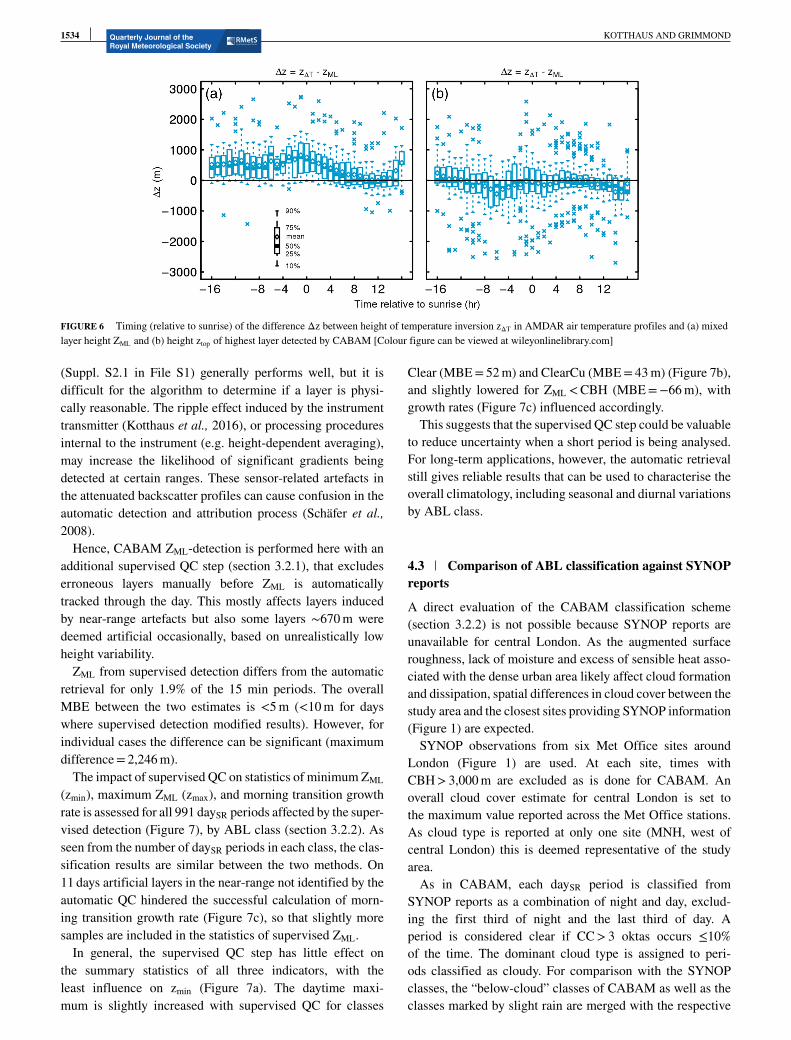
The median difference (Δz= zΔT −ZML) is 346 m based onall time periods; however, only 24 m for times >4 hr aftersunrise, as the two ABL estimates converge during the day(Figure 6a). CABAM not only detects ZML but also other lay-ers of significant gradient in attenuated backscatter (section3.2.1) so that the height ztop of the highest detected layer ineach measurement period can be compared to zΔT (Figure 6b).During daytime, ztop often agrees with ZML. However, at nightand early morning it frequently represents the top of the resid-ual layer. At night, zΔT has much better agreement with ztop

(Figure 6b) compared to ZML (Figure 6a), and hence seldommarks the top of the mixed layer.

4.2 Automatic versus supervised mixed layer heightdetection

At times the automatic ZML-detection selects erroneous layersthat are instrument-related noise or artefacts (Kotthaus et al.,2016) rather than atmospheric signatures. The QC moduledesigned to exclude artificial layers in the near range <200 m

1534 KOTTHAUS AND GRIMMOND

FIGURE 6 Timing (relative to sunrise) of the difference Δz between height of temperature inversion zΔT in AMDAR air temperature profiles and (a) mixedlayer height ZML and (b) height ztop of highest layer detected by CABAM [Colour figure can be viewed at wileyonlinelibrary.com]

(Suppl. S2.1 in File S1) generally performs well, but it isdifficult for the algorithm to determine if a layer is physi-cally reasonable. The ripple effect induced by the instrumenttransmitter (Kotthaus et al., 2016), or processing proceduresinternal to the instrument (e.g. height-dependent averaging),may increase the likelihood of significant gradients beingdetected at certain ranges. These sensor-related artefacts inthe attenuated backscatter profiles can cause confusion in theautomatic detection and attribution process (Schäfer et al.,2008).

Hence, CABAM ZML-detection is performed here with anadditional supervised QC step (section 3.2.1), that excludeserroneous layers manually before ZML is automaticallytracked through the day. This mostly affects layers inducedby near-range artefacts but also some layers ∼670 m weredeemed artificial occasionally, based on unrealistically lowheight variability.

ZML from supervised detection differs from the automaticretrieval for only 1.9% of the 15 min periods. The overallMBE between the two estimates is <5 m (<10 m for dayswhere supervised detection modified results). However, forindividual cases the difference can be significant (maximumdifference= 2,246 m).

The impact of supervised QC on statistics of minimum ZML

(zmin), maximum ZML (zmax), and morning transition growthrate is assessed for all 991 daySR periods affected by the super-vised detection (Figure 7), by ABL class (section 3.2.2). Asseen from the number of daySR periods in each class, the clas-sification results are similar between the two methods. On11 days artificial layers in the near-range not identified by theautomatic QC hindered the successful calculation of morn-ing transition growth rate (Figure 7c), so that slightly moresamples are included in the statistics of supervised ZML.

In general, the supervised QC step has little effect onthe summary statistics of all three indicators, with theleast influence on zmin (Figure 7a). The daytime maxi-mum is slightly increased with supervised QC for classes

Clear (MBE= 52 m) and ClearCu (MBE= 43 m) (Figure 7b),and slightly lowered for ZML <CBH (MBE=−66 m), withgrowth rates (Figure 7c) influenced accordingly.

This suggests that the supervised QC step could be valuableto reduce uncertainty when a short period is being analysed.For long-term applications, however, the automatic retrievalstill gives reliable results that can be used to characterise theoverall climatology, including seasonal and diurnal variationsby ABL class.

4.3 Comparison of ABL classification against SYNOPreports

A direct evaluation of the CABAM classification scheme(section 3.2.2) is not possible because SYNOP reports areunavailable for central London. As the augmented surfaceroughness, lack of moisture and excess of sensible heat asso-ciated with the dense urban area likely affect cloud formationand dissipation, spatial differences in cloud cover between thestudy area and the closest sites providing SYNOP information(Figure 1) are expected.

SYNOP observations from six Met Office sites aroundLondon (Figure 1) are used. At each site, times withCBH> 3,000 m are excluded as is done for CABAM. Anoverall cloud cover estimate for central London is set tothe maximum value reported across the Met Office stations.As cloud type is reported at only one site (MNH, west ofcentral London) this is deemed representative of the studyarea.

As in CABAM, each daySR period is classified fromSYNOP reports as a combination of night and day, exclud-ing the first third of night and the last third of day. Aperiod is considered clear if CC> 3 oktas occurs ≤10%of the time. The dominant cloud type is assigned to peri-ods classified as cloudy. For comparison with the SYNOPclasses, the “below-cloud” classes of CABAM as well as theclasses marked by slight rain are merged with the respective

KOTTHAUS AND GRIMMOND 1535

FIGURE 7 Three indicators of the mixed layer height ZML diurnal cycle,by major ABL classes (see section 3.2.2): (a) nocturnal minimum zmin, (b)daily maximum zmax, and (c) morning transition growth rate determinedfrom automatic and supervised CABAM detection for 991 daySR periodswhen supervised QC modified results. Number of daySR periods is givenabove each sub-plot

cloudy class. The “rain” class (complex precipitation doesnot permit successful detection of ZML) is excluded from thiscomparison.

Very good agreement between CABAM classes andSYNOP reports (Figure 8) is found for the Clear category(112 days, 88% total agreement), clear night followed by Cuday (151 days, 80%), and St (169 days, 58%). However, for theclass with highest occurrence, i.e. Cu during both night andday (456 days), a lot of the nights are classified as being clearby the ALC scheme so that the total agreement only reaches42%. In this case, agreement more than doubles (to 87%) ifonly daytime periods are considered. For all cloudy classes,agreement is significantly higher if only daytime periods arecompared.

Least agreement of only 20% is reached on the 5 days whenSYNOPs indicate a clear night followed by a day with St, asthe ALC classification mistakes the clouds for Cu. This islikely explained by the “morning bias” of the ALC schemewhich is centred around sunrise and a certain duration of theclouds is needed to be classified into St. If the St forms dur-ing the day or in the afternoon, the ALC scheme is not able todetect its stratiform nature.

The ALC scheme does not include a stratocumulus (SC)class. In the comparison (Figure 8), the 355 (460) periodsclassified as SC by SYNOPs during daytime (night-time) aremore likely to fall into the Cu category (day: 53%, night: 52%)rather than the St category (day: 33%, night: 20%) of the ALCclassification.

Considering the uncertainty introduced by the spatial rep-resentation of the SYNOP data to describe the central Londonarea, the CABAM classification scheme for ABL conditionscompares generally well to the observed cloud classes. Espe-cially the significant agreement during daytime suggests theALC-derived classes are sufficiently accurate to enhanceanalysis of the mixed layer height climatology (Kotthaus andGrimmond, 2018).

5 SUMMARY AND DISCUSSION

A novel algorithm for Characterising the AtmosphericBoundary layer (ABL) based on Automatic lidar and ceilome-ter (ALC) Measurements (CABAM) is presented. The tool iscapable of automatically tracking the mixed layer (ML) heightZML, filtering periods affected by complex rain patterns, andfurther classifies ABL characteristics into nights and daysaffected by clear sky, convective clouds, stratiform clouds,or ABL clouds that are present but the mixed layer remainsbelow cloud base height (CBH). Given ALC provide verticalprofiles of attenuated backscatter and automatic CBH detec-tion, they are very suitable to determine ABL characteristicsautomatically.

CABAM is designed for observations from the VaisalaCL31 ceilometer, an instrument which reaches completeoptical overlap by 70 m. Quality-control modules are imple-mented to reduce uncertainty induced by instrument noise andnear-range artefacts. With this careful processing, layers aslow as 50 m agl can be detected.

Application of CABAM to six years (2011–2016) of CL31observations in central London provides high-resolution(15 min, 10 m) results. Retrieved ZML is successfully eval-uated against inversion heights derived from temperatureprofiles of Aircraft Meteorological Data Relay (AMDAR).For a study area such as London with several planes perhour providing AMDAR data (here flights are extracted every15 min) there are advantages over the temporal resolutionof radiosonde profiles. Day-to-day comparison for clear-skydays has very good agreement in heights between CABAMmixed layer height and AMDAR temperature inversions, with

1536 KOTTHAUS AND GRIMMOND

FIGURE 8 Number of 24 hr periods (daySR) centred at sunrise classified into major ABL-classes: Clear, Cu, and St, based on ALC observations for day (fillcolour) and night (striped shading). ALC classes are grouped based on SYNOP categories (which also include a stratocumulus (SC) class). Number ofperiods in ALC class are normalised by total occurrence of the respective SYNOP class (no.of daySR periods). Agreement (%) is given for the total daySR

period and daytime only

a mean bias error (MBE) between 63 m in summer and 302 min winter during daytime. From time series analysis, it is evi-dent that significant scatter of the AMDAR-derived inversionheights is mostly responsible for the discrepancy in overallstatistics.

The presence of residual layers poses challenges to ZML

detection as upper boundaries of those layers above ML mightbe mistaken for ZML. While CABAM and AMDAR results arevery similar in the afternoon when the mixed layer often spansthe whole ABL, temperature inversions mark an elevatedlayer located above the CABAM-derived ZML during nightand the morning transition. The median difference betweeninversion heights and ZML is 346 m based on all time periods;however, only 24 m for times >4 hr after sunrise. In addi-tion to the mixed layer, CABAM tracks aerosol layers of theresidual layer that might be present above ZML. During night,the highest of these layers, presumably representing the top ofthe residual layer, shows good agreement with the AMDARinversion heights. The additional layers detected by CABAMcould be analysed in the future, for example, to evaluate theimpact of the residual layer on the morning transition growthrate. The latter is suggested to be increased when residual lay-ers are present (Blay-Carreras et al., 2014). Knowledge onresidual layers can also be valuable for the interpretation ofpollution concentrations observed within the ABL.

When compared to SYNOP/METAR reports, CABAM-derived ABL cloud classes are shown to compare very wellduring daytime. However, improvements might be possibleduring the night. Currently, CABAM assigns ABL categoriesbased on 24 hr periods. Results presented suggest it may bebeneficial to incorporate observations from the previous dayand subsequent night to improve identification of persistentstratiform clouds. Further, application of CABAM to otherregions where cloud types are different to southeast Englandcould help to improve the classification scheme. The cur-rent algorithm is considered to greatly benefit the analysis

of mixed layer height statistics (Kotthaus and Grimmond,2018), and provides the first ABL classification scheme thatdistinguishes cloud types solely based on ALC observations.

ACKNOWLEDGEMENTS

This study and ceilometer observations have received finan-cial support from EU FP7 BRIDGE, H2020 URBAN-FLUXES, NERC ClearfLo NE/H003231/1, NERC APHHChina AirPro NE/N00/00X/1, Newton Fund/ Met OfficeCSSP- China, EU COST Action TOPROF, King’s CollegeLondon and University of Reading. KCL and ERG/LAQN areacknowledged for providing site access. We thank CharleyStockdale, Lucia Monti, Duick Young, Chris Castillo, Kjellzum Berge, Will Morrison, Elliott Warren, Lukas Pauscher,Paul Smith, Tom Smith and all other staff and students atKCL and University of Reading who are involved in theLUMO measurement network. We also thank Max Priest-man and David Green at ERG for supporting the ceilometeroperation.

ORCID

Simone Kotthaus http://orcid.org/0000-0002-4051-0705C. Sue B. Grimmond http://orcid.org/0000-0002-3166-9415

REFERENCESBaars, H., Ansmann, A., Engelmann, R. and Althausen, D. (2008) Continuous

monitoring of the boundary-layer top with lidar. Atmospheric Chemistry andPhysics, 8, 7281–7296. https://doi.org/10.5194/acp-8-7281-2008.

Barlow, J.F. (2014) Progress in observing and modelling the urban boundary layer.Urban Climate, 10, 216–240. https://doi.org/10.1016/j.uclim.2014.03.011.

Barlow, J.F., Dunbar, T.M., Nemitz, E.G., Wood, C.R., Gallagher, M.W., Davies,F., O’Connor, E. and Harrison, R.M. (2011) Boundary layer dynamicsover London, UK, as observed using Doppler lidar during REPARTEE-II.Atmospheric Chemistry and Physics, 11, 2111–2125. https://doi.org/10.5194/acp-11-2111-2011.

KOTTHAUS AND GRIMMOND 1537

Biavati, G., Feist, D.G., Gerbig, C. and Kretschmer, R. (2015) Error estima-tion for localized signal properties: application to atmospheric mixing heightretrievals. Atmospheric Measurement Techniques, 8, 4215–4230. https://doi.org/10.5194/amt-8-4215-2015.

Blay-Carreras, E., Pino, D., Vilà-Guerau de Arellano, J., van de Boer, A., DeCoster, O., Darbieu, C., Hartogensis, O., Lohou, F., Lothon, M. and Pietersen,H. (2014) Role of the residual layer and large-scale subsidence on the develop-ment and evolution of the convective boundary layer. Atmospheric Chemistryand Physics, 14, 4515–4530. https://doi.org/10.5194/acp-14-4515-2014.

de Bruine, M., Apituley, A., Donovan, D.P., Klein Baltink, H. and de Haij,M.J. (2017) Pathfinder: applying graph theory to consistent tracking of day-time mixed layer height with backscatter lidar. Atmospheric MeasurementTechniques, 10, 1893–1909. https://doi.org/10.5194/amt-10-1893-2017.

Caicedo, V., Rappenglück, B., Lefer, B., Morris, G., Toledo, D. and Delgado,R. (2017) Comparison of aerosol lidar retrieval methods for boundary layerheight detection using ceilometer aerosol backscatter data. Atmospheric Mea-surement Techniques, 10, 1609–1622. https://doi.org/10.5194/amt-10-1609-2017.

Collaud Coen, M., Praz, C., Haefele, A., Ruffieux, D., Kaufmann, P. and Calpini,B. (2014) Determination and climatology of the planetary boundary layerheight above the Swiss plateau by in situ and remote sensing measurementsas well as by the COSMO-2 model. Atmospheric Chemistry and Physics, 14,13205–13221. https://doi.org/10.5194/acp-14-13205-2014.

Corripio, J.G. (2014) Insol: Solar Radiation. R package version 1.1.1. Availableat: https://CRAN.R-project.org/package=insol. [Accessed 12th March 2018]

Davies, F., Middleton, D.R. and Bozier, K.E. (2007) Urban air pollution modellingand measurements of boundary layer height. Atmospheric Environment, 41,4040–4049. https://doi.org/10.1016/j.atmosenv.2007.01.015.

Di Giuseppe, F., Riccio, A., Caporaso, L., Bonafé, G., Gobbi, G.P. and Angelini,F. (2012) Automatic detection of atmospheric boundary layer height usingceilometer backscatter data assisted by a boundary layer model. QuarterlyJournal of the Royal Meteorological Society, 138, 649–663. https://doi.org/10.1002/qj.964.

DWD. (2018) Ceilomap. Available at: http://www.dwd.de/EN/research/projects/ceilomap/ceilomap_node.html [Accessed 12th March 2018].

Emeis, S., Schäfer, K. and Münkel, C. (2008) Surface-based remote sensing ofthe mixing-layer height – a review. Meteorologische Zeitschrift, 17, 621–630.https://doi.org/10.1127/0941-2948/2008/0312.

Eresmaa, N., Härkönen, J., Joffre, S.M., Schultz, D.M., Karppinen, A. and Kukko-nen, J. (2012) A three-step method for estimating the mixing height usingceilometer data from the Helsinki testbed. Journal of Applied Meteorology andClimatology, 51, 2172–2187. https://doi.org/10.1175/JAMC-D-12-058.1.

Eresmaa, N., Karppinen, A., Joffre, S.M., Räsänen, J. and Talvitie, H. (2006) Mix-ing height determination by ceilometer. Atmospheric Chemistry and Physics,6, 1485–1493. https://doi.org/10.5194/acp-6-1485-2006.

Geiß, A. (2016) Automated calibration of ceilometer data and its applicabilityfor quantitative aerosol monitoring. PhD Thesis, LMU München. Availableat: https://edoc.ub.uni-muenchen.de/19930/1/Geiss_Alexander.pdf [Accessed12th March 2018].

Geiß, A., Wiegner, M., Bonn, B., Schäfer, K., Forkel, R., von Schneidemesser,E., Münkel, C., Chan, K.L. and Nothard, R. (2017) Mixing layer height asan indicator for urban air quality? Atmospheric Measurement Techniques, 10,2969–2988. https://doi.org/10.5194/amt-10-2969-2017.

Haeffelin, M., Angelini, F., Morille, Y., Martucci, G., Frey, S., Gobbi, G.P.,Lolli, S., O’Dowd, C.D., Sauvage, L., Xueref-Rémy, I., Wastine, B. and Feist,D.G. (2012) Evaluation of mixing-height retrievals from automatic profil-ing lidars and ceilometers in view of future integrated networks in Europe.Boundary-Layer Meteorology, 143, 49–75. https://doi.org/10.1007/s10546-011-9643-z.

de Haij, M., Wauben, W. and Klein Baltink, H. (2006) Determination of mixinglayer height from ceilometer backscatter profiles. In Proc. SPIE 6362, RemoteSensing of Clouds and the Atmosphere XI, 6362, 36–41. https://doi.org/10.1117/12.691050.

Haman, C.L., Lefer, B. and Morris, G.A. (2012) Seasonal variability in the diurnalevolution of the boundary layer in a near-coastal urban environment. Journal ofAtmospheric and Oceanic Technology, 29, 697–710. https://doi.org/10.1175/JTECH-D-11-00114.1.

Harvey, N.J., Hogan, R.J. and Dacre, H.F. (2013) A method to diag-nose boundary-layer type using Doppler lidar. Quarterly Journal ofthe Royal Meteorological Society, 139, 1681–1693. https://doi.org/10.1002/qj.2068.

Hervo, M., Poltera, Y. and Haefele, A. (2016) An empirical method to correct fortemperature dependent variations in the overlap function of CHM15k ceilome-ters. Atmospheric Measurement Techniques, 7, 2947–2959. https://doi.org/10.5194/amt-9-2947-2016.

Knippertz, P. and Stuut, J.-B.W. (Eds.). (2014) Mineral Dust: A Key Player inthe Earth System. Netherlands: Springer. https://doi.org/10.1007/978-94-017-8978-3.

Kotthaus, S. and Grimmond, C.S.B. (2018) Atmospheric boundary-layer char-acteristics from ceilometer measurements. Part 2: Application to London’surban boundary layer. Q J R Meteorol Soc 2018;1–13. https://doi.org/10.1002/qj.3298

Kotthaus, S., O’Connor, E., Münkel, C., Charlton-Perez, C., Haeffelin, M., Gabey,A.M. and Grimmond, C.S.B. (2016) Recommendations for processing atmo-spheric attenuated backscatter profiles from Vaisala CL31 ceilometers. Atmo-spheric Measurement Techniques, 9, 3769–3791. https://doi.org/10.5194/amt-9-3769-2016.

Lammert, A. and Bösenberg, J. (2006) Determination of the convectiveboundary-layer height with laser remote sensing. Boundary-Layer Meteorol-ogy, 119, 159–170. https://doi.org/10.1007/s10546-005-9020-x.

Lotteraner, C. and Piringer, M. (2016) Mixing-height time series from opera-tional ceilometer aerosol-layer heights. Boundary-Layer Meteorology, 161,265–287. https://doi.org/10.1007/s10546-016-0169-2.

Madonna, F., Amato, F., Vande Hey, J. and Pappalardo, G. (2015) Ceilometeraerosol profiling versus Raman lidar in the frame of the INTERACT campaignof ACTRIS. Atmospheric Measurement Techniques, 8, 2207–2223. https://doi.org/10.5194/amt-8-2207-2015.

Markowicz, K.M., Flatau, P.J., Kardas, A.E., Remiszewska, J., Stelmaszczyk, K.and Woeste, L. (2008) Ceilometer retrieval of the boundary layer verticalaerosol extinction structure. Journal of Atmospheric and Oceanic Technology,25, 928–944. https://doi.org/10.1175/2007JTECHA1016.1.

Martucci, G., Matthey, R., Mitev, V. and Richner, H. (2007) Comparison betweenbackscatter lidar and radiosonde measurements of the diurnal and nocturnalstratification in the lower troposphere. Journal of Atmospheric and OceanicTechnology, 24, 1231–1244. https://doi.org/10.1175/JTECH2036.1.

Martucci, G., Milroy, C. and O’Dowd, C.D. (2010) Detection of cloud-baseheight using Jenoptik CHM15K and Vaisala CL31 ceilometers. Journal ofAtmospheric and Oceanic Technology, 27, 305–318. https://doi.org/10.1175/2009JTECHA1326.1.

Marzano, F.S., Mereu, L., Montopoli, M., Cimini, D. and Martucci, G. (2014)Volcanic ash cloud observation using ground-based Ka-band radar andnear-infrared lidar ceilometer during the Eyjafjallajökull eruption. Annals ofGeophysics, 57, 1–7. https://doi.org/10.4401/ag-6634.

Met Office. (2008) AMDAR (Aircraft Meteorological Data Relay) reportsCollected by the Met Office MetDB System. NCAS British Atmo-spheric Data Centre. Available at: http://catalogue.ceda.ac.uk/uuid/220a65615218d5c9cc9e4785a3234bd0 [Accessed 12 March 2018].

Met Office. (2012) Met Office Integrated Data Archive System (MIDAS) Landand Marine Surface Stations Data (1853-current). NCAS British AtmosphericData Centre. Available at: http://badc.nerc.ac.uk/browse/badc/ukmo-midas[Accessed 12 March 2018].

Mielonen, T., Aaltonen, V., Lihavainen, H., Hyvärinen, A.-P., Arola, A., Komp-pula, M. and Kivi, R. (2013) Biomass burning aerosols observed in northernFinland during the 2010 wildfires in Russia. Atmosphere, 4, 17–34. https://doi.org/10.3390/atmos4010017.

Morille, Y., Haeffelin, M., Drobinski, P. and Pelon, J. (2007) STRAT: an auto-mated algorithm to retrieve the vertical structure of the atmosphere fromsingle-channel lidar data. Journal of Atmospheric and Oceanic Technology,24, 761–775. https://doi.org/10.1175/JTECH2008.1.

Münkel, C. (2016) Combining gradient and profile fit method for an advancedceilometer-based boundary layer height detection algorithm, ISARS2016,Varna, Bulgaria, 6–9 June 2016.

Münkel, C., Eresmaa, N., Räsänen, J. and Karppinen, A. (2007) Retrieval ofmixing height and dust concentration with lidar ceilometer. Boundary-LayerMeteorology, 124, 117–128. https://doi.org/10.1007/s10546-006-9103-3.

Nemuc, A., Stachlewska, I.S., Vasilescu, J., Górska, A., Nicolae, D. and Tal-ianu, C. (2014) Optical properties of long-range transported volcanic ashover Romania and Poland during Eyjafjallajökull eruption in 2010. ActaGeophysica, 62, 350–366. https://doi.org/10.2478/s11600-013-0180-7.

Pal, S. and Haeffelin, M. (2015) Forcing mechanisms governing diurnal, sea-sonal, and interannual variability in the boundary layer depths: five yearsof continuous lidar observations over a suburban site near Paris. Journal of

1538 KOTTHAUS AND GRIMMOND

Geophysical Research: Atmospheres, 120, 11936–11956. https://doi.org/10.1002/2015JD023268.

Pal, S., Haeffelin, M. and Batchvarova, E. (2013) Exploring a geophysicalprocess-based attribution technique for the determination of the atmosphericboundary layer depth using aerosol lidar and near-surface meteorological mea-surements. Journal of Geophysical Research: Atmospheres, 118, 9277–9295.https://doi.org/10.1002/jgrd.50710.

Pearson, G., Davies, F. and Collier, C. (2010) Remote sensing of the tropical rainforest boundary layer using pulsed Doppler lidar. Atmospheric Chemistry andPhysics, 10, 5891–5901. https://doi.org/10.5194/acp-10-5891-2010.

Peng, J., Grimmond, C.S.B., Fu, X., Chang, Y., Zhang, G., Guo, J., Tang, C., Gao,J., Xu, X. and Tan, J. (2017) Ceilometer based analysis of Shanghai’s bound-ary layer height (under rain and fog free conditions). Journal of Atmosphericand Oceanic Technology, 34, 749–764. https://doi.org/10.1175/JTECH-D-16-0132.1.

Piringer, M., Joffre, S., Baklanov, A., Christen, A., Deserti, M., Ridder, K., Emeis,S., Mestayer, P., Tombrou, M., Middleton, D., Baumann-Stanzer, K., Dan-dou, A., Karppinen, A. and Burzynski, J. (2007) The surface energy balanceand the mixing height in urban areas – activities and recommendations ofCOST-Action 715. Boundary-Layer Meteorology, 124, 3–24. https://doi.org/10.1007/s10546-007-9170-0.

Poltera, Y., Martucci, G., Collaud Coen, M., Hervo, M., Emmenegger, L.,Henne, S., Brunner, D. and Haefele, A. (2017) PathfinderTURB: an auto-matic boundary layer algorithm. Development, validation and application tostudy the impact on in situ measurements at the Jungfraujoch. AtmosphericChemistry and Physics, 17, 10051–10070. https://doi.org/10.5194/acp-17-10051-2017.

R Core Team. (2017) R: a language and environment for statistical computing.Vienna: R Foundation for Statistical Computing. Retrieved from https://www.R-project.org/.

Rahn, D.A. and Mitchell, C.J. (2016) Diurnal climatology of the boundary layerin southern California using AMDAR temperature and wind profiles. Journalof Applied Meteorology and Climatology, 55, 1123–1137. https://doi.org/10.1175/JAMC-D-15-0234.1.

Schäfer, K., Emeis, S., Jahn, C., Münkel, C., Schrader, S. and Höß, M. (2008)New results from continuous mixing layer height monitoring in urban atmo-sphere. Proceedings of SPIE, Remote Sensing of Clouds and the AtmosphereXIII, 7107, 71070A. https://doi.org/10.1117/12.800358.

Schäfer, K., Emeis, S.M., Rauch, A., Munkel, C. and Vogt, S. (2004) Determina-tion of the mixing layer height from ceilometer backscatter profiles. RemoteSensing of Clouds and the Atmosphere IX, 5571, 248–259. https://doi.org/10.1117/12.565592.

Schween, J.H., Hirsikko, A., Löhnert, U. and Crewell, S. (2014) Mixing-layerheight retrieval with ceilometer and Doppler lidar: from case studies tolong-term assessment. Atmospheric Measurement Techniques, 7, 3685–3704.https://doi.org/10.5194/amt-7-3685-2014.

Sokół, P., Stachlewska, I., Ungureanu, I. and Stefan, S. (2014) Evaluation of theboundary layer morning transition using the CL-31 ceilometer signals. ActaGeophysica, 62, 367–380. https://doi.org/10.2478/s11600-013-0158-5.

Stachlewska, I.S., Pi ¸adłowski, M., Migacz, S., Szkop, A., Zielinska, A.J. andSwaczyna, P.L. (2012) Ceilometer observations of the boundary layer overWarsaw, Poland. Acta Geophysica, 60, 1386–1412. https://doi.org/10.2478/s11600-012-0054-4.

Steyn, D.G., Baldi, M. and Hoff, R.M. (1999) The detection of mixedlayer depth and entrainment zone thickness from lidar backscatter pro-files. Journal of Atmospheric and Oceanic Technology, 16, 953–959.https://doi.org/10.1175/1520-0426(1999)016<0953:TDOMLD>2.0.CO;2.

Stull, R.B. (1988) An Introduction to Boundary Layer Meteorology. Dordrecht:Kluwer Academic Publishers.

Tang, G., Zhang, J., Zhu, X., Song, T., Münkel, C., Hu, B., Schäfer, K., Liu, Z.,Zhang, J., Wang, L., Xin, J., Suppan, P. and Wang, Y. (2016) Mixing layerheight and its implications for air pollution over Beijing, China. AtmosphericChemistry and Physics, 16, 2459–2475. https://doi.org/10.5194/acp-16-2459-2016.

Tsaknakis, G., Papayannis, A., Kokkalis, P., Amiridis, V., Kambezidis, H.D.,Mamouri, R.E., Georgoussis, G. and Avdikos, G. (2011) Inter-comparisonof lidar and ceilometer retrievals for aerosol and planetary boundary layerprofiling over Athens, Greece. Atmospheric Measurement Techniques, 4,1261–1273. https://doi.org/10.5194/amt-4-1261-2011.

Van der Kamp, D. and McKendry, I. (2010) Diurnal and seasonal trends in con-vective mixed-layer heights estimated from two years of continuous ceilometerobservations in Vancouver, BC. Boundary-Layer Meteorology, 137, 459–475.https://doi.org/10.1007/s10546-010-9535-7.

Wagner, P. and Schäfer, K. (2017) Influence of mixing layer height on air pollutantconcentrations in an urban street canyon. Urban Climate, 22, 64–79. https://doi.org/10.1016/j.uclim.2015.11.001.

Wiegner, M., Emeis, S., Freudenthaler, V., Heese, B., Junkermann, W., Münkel,C., Schäfer, K., Seefeldner, M. and Vogt, S. (2006) Mixing layer heightover Munich, Germany: variability and comparisons of different methodolo-gies. Journal of Geophysical Research, 111, D13201. https://doi.org/10.1029/2005JD006593.

Wiegner, M. and Gasteiger, J. (2015) Correction of water vapor absorption foraerosol remote sensing with ceilometers. Atmospheric Measurement Tech-niques, 8, 3971–3984. https://doi.org/10.5194/amt-8-3971-2015.

Wiegner, M., Gasteiger, J., Groß, S., Schnell, F., Freudenthaler, V. and Forkel, R.(2012) Characterization of the Eyjafjallajökull ash-plume: potential of lidarremote sensing. Physics and Chemistry of the Earth, Parts A/B/C, 45–46,79–86. https://doi.org/10.1016/j.pce.2011.01.006.

SUPPORTING INFORMATION

Additional supporting information may be found online in theSupporting Information section at the end of the article.

How to cite this article: Kotthaus S, Grimmond CSB.Atmospheric boundary-layer characteristics fromceilometer measurements. Part 1: A new methodto track mixed layer height and classify clouds.Q J R Meteorol Soc 2018;144:1525–1538.https://doi.org/10.1002/qj.3299