ATHEMATICAL MODELLING OF TUBE HEAT...

Chemical and Process Engineering 2011, 32 ( 1), 7-19

DOI: 10.2478/v10176-011-0001-y

*Corresponding author, e-mail: [email protected]

7

MATHEMATICAL MODELLING OF TUBE HEAT EXCHANGERS WITH COMPLEX FLOW ARRANGEMENT

Dawid Taler1*, Marcin Trojan2, Jan Taler2 1Cracow University of Science And Technology (AGH), Department of Power Energy Systems and Environment Protection, Faculty of Mechanical Engineering And Robotics, Cracow, Poland 2Cracow University of Technology, Department of Power Plant Machinery, Institute of Process and Power Engineering, Cracow, Poland

General principles of mathematical modelling of transient heat transfer in cross-flow tube heat exchangers with complex flow arrangements which allow a simulation of multipass heat exchangers with many tube rows are presented. First, a system of differential equations for the transient temperature of both fluids and the tube wall with appropriate boundary and initial conditions is formulated. Two methods for modelling heat exchangers are developed using the finite difference method and finite volume method. A numerical model of multipass steam superheater with twelve passes is presented. The calculation results are compared with the experimental data.

Keywords: heat tube exchanger, modelling, complex flow

1. INTRODUCTION

Cross-flow tube heat exchangers find many practical applications. An example of such an exchanger is a steam superheater , where steam flows inside the tubes while heating flue gas flows across the tube bundles. The mathematical derivation of an expression for the mean temperature difference becomes quite complex for multi-pass cross-flow heat exchangers with many tube rows and complex flow arrangement (Hewitt et al., 1994; Kröger, 1998; Rayaprolu, 2009; Stultz and Kitto, 1992; Taler, 2009). When calculating the heat transfer rate, the usual procedure is to modify the simple counter-flow LMTD (Logarithmic Mean Temperature Difference) method by a correction FT determined for a particular arrangement. The heat flow rate Q& transferred from the hot to cool fluid is the product of the overall heat transfer coefficient UA, heat transfer area A, correction factor FT and logarithmic mean temperature difference ΔTlm. The heat transfer equation then takes the form:

A T lmQ U A F T= Δ& . (1)

However, to calculate steam , flue gas and wall temperature distributions, a numerical model of the superheater is indispensable. Superheaters are tube bundles that attain the highest temperatures in a boiler and consequently require the greatest care in the design and operation. The complex superheater tube arrangements permit an economic trade-off between material unit costs and surface area required to obtain the prescribed steam outlet temperature. Very often, various alloy steels are used for each pass in modern boilers.

D. Taler, M. Trojan, J. Taler, Chem. Process Eng., 2011, 32 ( 1), 7-19

8

High temperature heat exchangers like steam superheaters are difficult to model since the tubes receive energy from the flue gas by two heat transfer modes: convection and radiation. The division of superheaters into two types: convection and radiant superheaters is based on the mode of heat transfer that is predominant. In convection superheaters, the portion of heat transfer by radiation from the flue gas is small. A radiant superheater absorbs heat primarily by thermal radiation from the flue gas with little convective heat flow rate. The share of convection in the total heat exchange of platen superheaters located directly over the combustion chamber amounts only to 10 to 15% . In convective superheaters, the share of radiation heat exchange is lower, but cannot be neglected.

Correct determination of the heat flux absorbed through the boiler heating surfaces is very difficult. This is due, on the one hand, to the complexity of heat transfer by radiation of flue gas with a high content of solid ash particles, and on the other hand, to the fouling of heating surfaces by slag and ash (Taler et al., 2009). The degree of the slag and ash deposition is hard to assess, both at the design stage and during the boiler operation. In consequence, the proper size of superheaters can be adjusted only after the boiler start-up. In cases when the temperature of superheated steam at the exit from the superheater stage under examination is higher than its design value, then the area of the surface of this stage has to be decreased. However, if the exit temperature of the steam is below the desired value, then the surface area is increased.

2. MATHEMATICAL MODEL OF THE SUPERHEATER

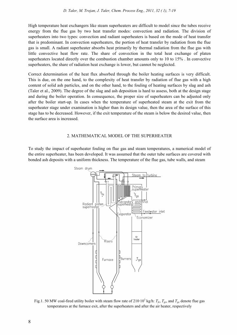
To study the impact of superheater fouling on flue gas and steam temperatures, a numerical model of the entire superheater, has been developed. It was assumed that the outer tube surfaces are covered with bonded ash deposits with a uniform thickness. The temperature of the flue gas, tube walls, and steam

Fig.1. 50 MW coal-fired utility boiler with steam flow rate of 210·103 kg/h: Tfe, Tgs, and Tge denote flue gas temperatures at the furnace exit, after the superheaters and after the air heater, respectively

Mathematical modelling of tube heat exchangers with the complex flow arrangement

9

was determined using the finite volume method (FVM) (Taler, 2009). Subsequent stages of the superheater were modeled as either cross-parallel-flow or cross-counter-flow. As an example, a numerical model of the first stage convective will be presented in detail (Figs. 1 and 2). The first stage convective superheater is a pendant twelve-pass heat exchanger.

The superheater is constructed of circular bare tubes and is situated at the back of the second and third stages of the superheater (Figs. 1 and 2). The tube is made of grade St 20 carbon steel, having a 42 mm outside diameter and 5mm thick wall. The superheated steam and the combustion products flow at right angles to each other. The convective superheater considered in the paper can be classified according to flow arrangement as a mixed-cross-flow heat exchanger (Figs. 2 and 3). Each individual pass consists of two tubes through which superheated steam flows parallel (Fig. 2).

Fig. 2. Arrangement of boiler heating surfaces

Based on the energy conservation principle, a mathematical model of steam superheater with 12 tube rows and complex flow arrangement was developed. The radiant and convective superheaters are located in boiler passes through which high temperature flue gas flows. The gas temperature drops from about 1100 °C at the exit of the furnace chamber to about 400 °C before entering the economizer. Radiant platen superheaters are located in areas of highest flue gas temperature, and the water heater in the lowest temperature pass. To calculate the radiation heat transfer from the hot flue gases to the tubes, it is necessary to solve the radiative heat transfer equation (Taler and Taler, 2009).

3. MATHEMATICAL MODEL OF ONE ROW TUBE HEAT EXCHANGER

A mathematical model of the cross flow tubular heat exchanger, in which air or flue gas flows transversally through a row of tubes will be developed. The system of partial differential equations


10

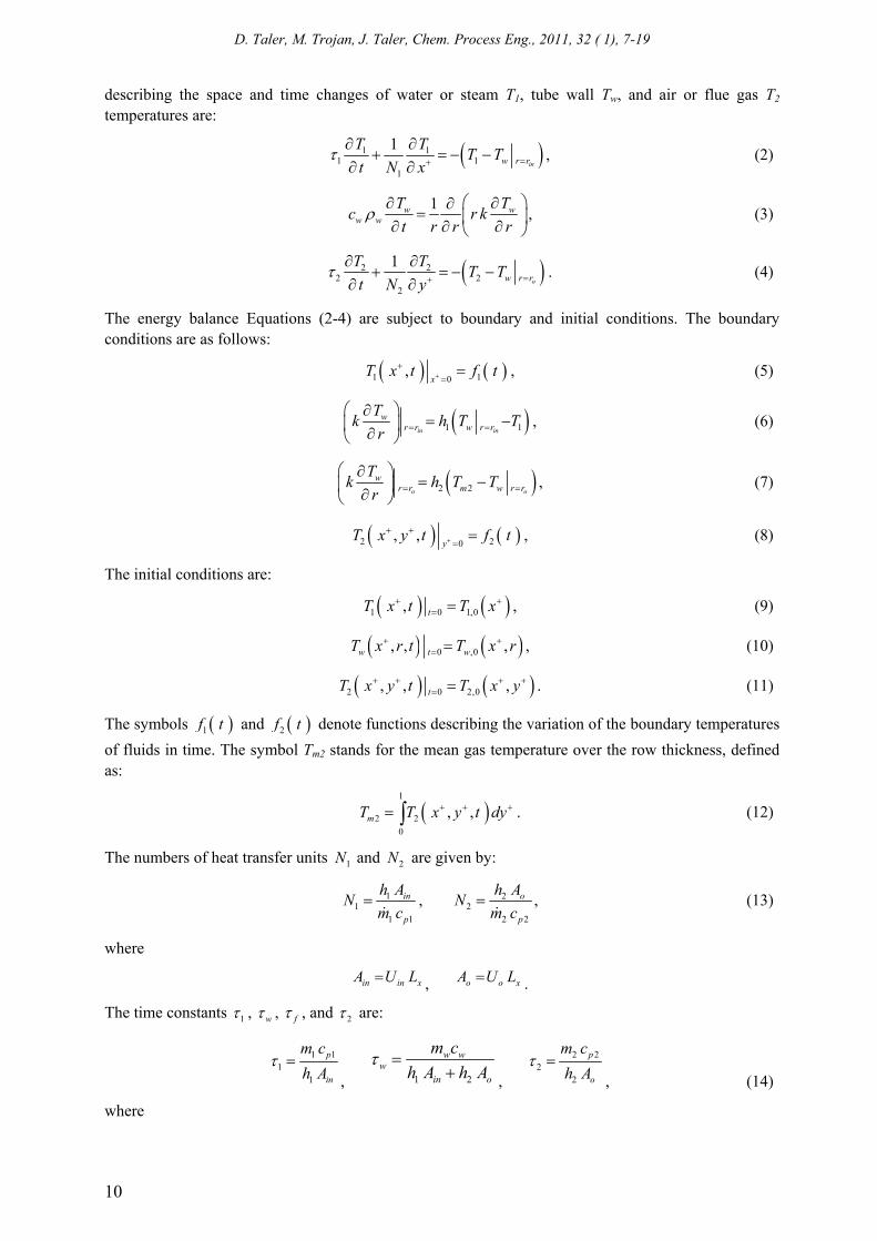
describing the space and time changes of water or steam T1, tube wall Tw, and air or flue gas T2 temperatures are:

( )1 11 1

1

1inw r r

T T T Tt N x

τ =+

∂ ∂+ = − −

∂ ∂, (2)

1w ww w

T Tc r kt r r r

ρ⎛ ⎞∂ ∂∂

= ⎜ ⎟∂ ∂ ∂⎝ ⎠, (3)

( )2 22 2

2

1ow r r

T T T Tt N y

τ =+

∂ ∂+ = − −

∂ ∂. (4)

The energy balance Equations (2-4) are subject to boundary and initial conditions. The boundary conditions are as follows:

( ) ( )1 10,

xT x t f t+

+== , (5)

( )1 1in in

wr r w r r

Tk h T Tr = =

⎛ ⎞∂= −⎜ ⎟∂⎝ ⎠

, (6)

( )2 2o o

wr r m w r r

Tk h T Tr = =

⎛ ⎞∂= −⎜ ⎟∂⎝ ⎠

, (7)

( ) ( )2 20, ,

yT x y t f t+

+ +== , (8)

The initial conditions are:

( ) ( )1 0 1,0, tT x t T x+ += = , (9)

( ) ( )0 ,0, , ,w t wT x r t T x r+ += = , (10)

( ) ( )2 0 2,0, , ,tT x y t T x y+ + + += = . (11)

The symbols ( )1f t and ( )2f t denote functions describing the variation of the boundary temperatures of fluids in time. The symbol Tm2 stands for the mean gas temperature over the row thickness, defined as:

( )1

2 20

, ,mT T x y t dy+ + += ∫ . (12)

The numbers of heat transfer units 1N and 2N are given by:

11

1 1

in

p

h ANm c

=&

, 22

2 2

o

p

h ANm c

=&

, (13)

where

in in xA U L= , o o xA U L= .

The time constants 1τ , wτ , fτ , and 2τ are:

1 11

1

p

in

m ch A

τ =, 1 2

w ww

in o

m ch A h A

τ =+ ,

2 22

2

p

o

m ch A

τ =, (14)

where


11

1 1in xm A L ρ= , 2

2 1 2 24o

xdm s s Lπ

ρ⎛ ⎞

= −⎜ ⎟⎝ ⎠

, w m w x wm U Lδ ρ= , ( ) / 2m in oU U U= +

The transient fluids and wall temperature distributions in one row heat exchanger (Fig. 3) are then determined by the explicit finite difference method.

3.1. Transient model of one row tube heat exchanger

Transient distributions of fluid and tube wall temperatures were determined using an explicit finite-difference method. The tube wall was divided into three control volumes (Fig. 3). The finite difference cell is shown in Fig. 3.

Fig. 3. Control volume for one-row cross-flow tube heat exchanger

Approximating Eq.(2) using the explicit finite difference method gives:

1, 1, 11, 1 1,11, 1 1, 1 ,

1, 1, 1, 2

n nn ni ii in n n

i i ww in n ni i i

T TT Tt tT T TN xτ τ

++++ + +

⎛ ⎞+−Δ Δ= − − −⎜ ⎟⎜ ⎟Δ ⎝ ⎠

, Ni ,...,1= , ,...1,0=n , (15)

The finite volume method (Taler, 2009) was used to solve Eq. (3). The ordinary differential equations for wall temperatures at nodes were solved using the explicit Euler method to obtain:

( )

( )

( ) ( )

( )

1, , ,

1, 1, 1, 1 , , ,

, , 022 2

2 /2

n n nww i ww i wm i

n ni in n n n n

wm i wm i ww i ww in nwm i ww i

w w

T T T

T TT h r k T T T

T T rrtr rr r

α+

+

= + ×

⎧ ⎫⎛ ⎞+⎡ ⎤− ⋅Δ − −⎪ ⎪⎜ ⎟⎣ ⎦ ⎜ ⎟−⎪ ⎪⎝ ⎠×Δ +⎨ ⎬

Δ Δ⎪ ⎪⎪ ⎪⎩ ⎭

(16)

( )( ) ( ), , , ,1 3 2

, , , 2 22 3 2 3

2 2n n n nwz i wm i ww i wm in n n

wm i wm i wm i

T T T Tr rT T T tr r r rr r

α+⎡ ⎤− −

= + Δ ⋅ +⎢ ⎥+ +Δ Δ⎢ ⎥⎣ ⎦

, (17)


12

( )

( ) ( ) ( ) ( )

( ) ( )

1, , ,

' ''2, 2,

, 2 , , ,

, ,5 32 2

2 /2

n n nwz i wz i wm i

n n

i in n n n nwm i wm i wz i wz i

n nwm i wz i

z z

T T T

T TT h r k T T T

T Tr rtr rr r

α+ = + ×

⎧ ⎫⎡ ⎤+⎪ ⎪⎢ ⎥⎡ ⎤+ ⋅ Δ − −⎣ ⎦⎪ ⎪⎢ ⎥ −⎪ ⎪⎣ ⎦×Δ +⎨ ⎬Δ Δ⎪ ⎪

⎪ ⎪⎪ ⎪⎩ ⎭

(18)

Solving Eq. (4) using the explicit Euler method gives the temperature of the fluid 2 at the exit of the finite volume (Fig. 3):

( ) ( ) ( ) ( ) ( ) ( )' ''1 2, 2,'' '' ' ''

2, 2, 2, 2, ,2, 2, 2, 2

n nn n n n i in

i i i i wz in n ni i i

T Tt tT T T T TN τ τ

+⎡ ⎤+Δ Δ⎡ ⎤ ⎢ ⎥= + − + −⎢ ⎥⎣ ⎦ ⎢ ⎥⎣ ⎦

, Ni ,...,1= , ,...1,0=n (19)

The initial temperature distributions for the fluid 1 and 2 are given by Equations (9-11), which can be written as:

0, 0 ,ww i t ww iT T= = , 0

, 0 ,wm i t wm iT T= = , 0, 0 ,wz i t wz iT T= = , Ni ,...,1= , (20)

where the symbols 0,ww iT , 0

,wm iT , and 0,wz iT denote the wall temperatures at the nodes.

The boundary conditions for fluids are given by Equations (5) and (8). The presented finite difference method is accurate and easy to program. In order to assure the stability of the calculations, the Courant conditions for both fluids and the stability condition for the Fourier equation defining transient heat conduction in the tube wall, should be satisfied.

4. MATHEMATICAL MODEL OF CONVECTIVE SUPERHEATER

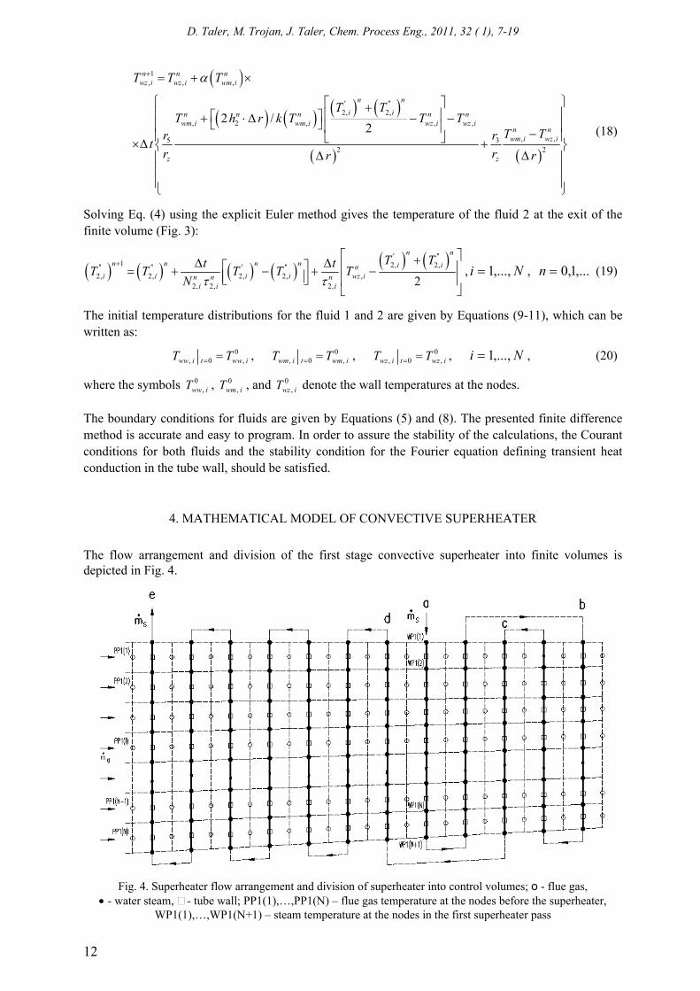
The flow arrangement and division of the first stage convective superheater into finite volumes is depicted in Fig. 4.

Fig. 4. Superheater flow arrangement and division of superheater into control volumes; o - flue gas, • - water steam, - tube wall; PP1(1),…,PP1(N) – flue gas temperature at the nodes before the superheater,

WP1(1),…,WP1(N+1) – steam temperature at the nodes in the first superheater pass


13

The superheated steam and the combustion products flow at right angles to each other. The first stage of a convective superheater can be classified according to flow arrangement as a mixed-cross-flow heat exchanger. The superheater tubes are arranged in-line (Fig. 5b). Each individual pass consists of two tubes through which superheated steam flows parallel. The tube’s outer surface is covered with a layer of ash deposits. In the following , finite volume heat balance equations will be formulated for the steam, the tube wall, and the flue gas. A steam side energy balance for the ith finite volume gives (Fig. 5a):

, , 1, , 1, 1, , 10 0

2

s i s iT Ts i s is ps s i in s w i s ps s i

T Tm c T d x h T m c Tπ ++

+

⎛ ⎞++ Δ − =⎜ ⎟⎜ ⎟

⎝ ⎠& & . (21)

Rearranging Eq. (21) gives

( ), 1

,

, , 1, 1 , 1,

2

s i

s i

T s i s is ps s i s i in s w iT

T Tm c T T A h T+ +

+

⎛ ⎞+− =Δ −⎜ ⎟⎜ ⎟

⎝ ⎠& , (22)

where the mesh tube inner surface is

in inA d xπΔ = Δ . (23)

The steam average specific heat at constant pressure is given by:

( ) ( ), 1

,

, , 1,

2s i

s i

T ps s i ps s ips ps iT

c T c Tc c+ ++

≈ = . (24)

After rewriting Eq. (22) in the form

, 1 , , 1,

,

11 22

s i s ps i s in s i s in w i

s ps i s in

T m c h A T h A Tm c h A

+

⎡ ⎤⎛ ⎞= − Δ + Δ⎢ ⎥⎜ ⎟⎜ ⎟⎢ ⎥⎝ ⎠+ Δ ⎣ ⎦

&&

i = 1,…, N, (25)

the Gauss-Seidel method can be applied for an iterative solving nonlinear set of algebraic equations (25). Introducing the mesh number of transfer units for the steam:

( ) ( )

1,2 , , , 1

2s in s in

s is ps i s ps s i ps s i

h A h ANm c m c T c T+

+

Δ ΔΔ = =

⎡ ⎤+⎣ ⎦& &. (26)

and dividing Eq. (26) by ,s ps im c& , we have:

, 1 1 , 1 1,, ,2 21,

2

1 11 , 1, ... ,1 212

s i s i w is i s i

s i

T N T N T i NN

++ +

+

⎡ ⎤⎛ ⎞⎢ ⎥⎜ ⎟= − Δ + Δ =⎜ ⎟⎢ ⎥+ Δ ⎝ ⎠⎣ ⎦

. (27)

where: /xx L NΔ = - the mesh size, Lx – the tube length.

The energy conservation principle for the flue gas applied for the finite control volume (Fig. 5) is:

( )' ", ,

' ", ,' "

, , 3,0 02 2

2

g i g iT T g i g ig pg g i g pg g i o z g w i

T Tm c T m c T r x h Tπ δ

⎛ ⎞+Δ = Δ + + Δ −⎜ ⎟⎜ ⎟

⎝ ⎠& & . (28)

After rearranging Eq. (28), we obtain:

( )' ", ,' "

, , , 3,2

g i g ig pg i g i g i z g w i

T Tm c T T A h T

⎛ ⎞+Δ − = Δ −⎜ ⎟⎜ ⎟

⎝ ⎠& (29)


14

where the mesh outer surface of deposits is (Fig. 6):

( )2 2z o zA r xπ δΔ = + Δ (30)

The flue gas average specific heat at constant pressure is given by:

( ) ( )" '

, ,,

2

pg g i pg g ipg i

c T c Tc

+= (31)

Fig. 5. Finite volume for energy balance on the steam and gas sides (a) and in-line array of superheater tubes (b)

Equation (29) can be written as:

" ', , , 3,

,

1 11 22

g i g pg i g z g i g z w i

g pg i g z

T m c h A T h A Tm c h A

⎡ ⎤⎛ ⎞= Δ − Δ + Δ⎢ ⎥⎜ ⎟⎜ ⎟⎢ ⎥⎝ ⎠⎣ ⎦Δ + Δ

&

& (32)

Introducing the mesh number of transfer units for the gas:

( ) ( )1 ' ",

2 , , ,

2g z g z

g ig pg i g pg g i pg g i

h A h AN

m c m c T c T+

Δ ΔΔ = =

⎡ ⎤Δ Δ +⎣ ⎦& & (33)

and dividing Eq. (33) by ,g pg im c& we obtain:

" ', 1 , 1 3,, ,

2 21,2

1 11 , 1, ... , .1 212

g i g i w ig i g i

g i

T N T N T i NN + +

+

⎡ ⎤⎛ ⎞⎢ ⎥⎜ ⎟= − Δ + Δ =⎜ ⎟⎢ ⎥+ Δ ⎝ ⎠⎣ ⎦

(34)

Subsequently, energy conservation equations for the tube wall (Fig. 6) will be written. The tube wall and the deposit layer are divided into three finite volumes (Fig. 7).

Energy conservation equations may be written as:

node 1

( ) ( ) ( )1, 2, 2, 1,, 1, 0

2

w w i w w i w i w is s i w i in c

w

k T k T T Th T T d dπ π

δ

+ −− + = (35)

where: ( ) , , 1,/ 2 ,

2

s i s ic in o in o s i

T Td d d r r T ++

= + = + = .

a) b)


15

Fig. 6. Tube wall with a layer of deposits at the outer tube surfaces

Fig. 7. Division of the tube wall and deposit layer into three control volumes

node 2

( ) ( )1, 2, 1, 2, 3, 2, 0

2

w w i w w i w i w i w i w ic z s

w z

k T k T T T T Td k dπ π

δ δ

+ − −+ = (36)

where: 2s o z o zd d rδ δ= + = + .

node 3

( ) ( ) 2, 3,, 3, 2 0w i w i

g g i w i o z z s

z

T Th T T d k dπ δ π

δ

−− + + = (37)

Algebraic equations (35) – (37) can be rewritten in a form which is suitable for solving equation sets by using the Gauss – Seidel method:

( ) ( )

( ) ( )1, 2,1, , 2

1, 2,

1

2

2

w w i w w i cw i s s i in w

w w i w w i c ws in

w

k T k T dT h T d Tk T k T dh d δ

δ

⎡ ⎤+⎢ ⎥= +⎢ ⎥+ ⎣ ⎦+

(38)


16

( ) ( )

( ) ( )1, 2,2, 1, 3,

1, 2,

1

2

2

w w i w w i c sw i w i z w i

w w i w w i c z w zs

w z

k T k T d dT T k Tk T k T d k d δ δ

δ δ

⎡ ⎤+⎢ ⎥= +⎢ ⎥+ ⎣ ⎦+

(39)

( )( )3, , 2,

1 2

2

sw i g o z g i z w i

zsg o z z

z

dT h d T k Tdh d k

δδ

δδ

⎡ ⎤⎢ ⎥= + +

⎡ ⎤ ⎢ ⎥⎣ ⎦⎢ ⎥+ +

⎢ ⎥⎣ ⎦

(40)

Equations (38) – (40) can be used for building mathematical models of steam superheaters. To solve Eqs. (27), (34) and (38) – (40) two boundary conditions are prescribed: inlet steam temperature ,s inletT and flue gas temperature ,g inletT before the superheater:

,1(1) s inletWP T= and ,1( ) , 1,...,g inletPP I T I N= = . (41)

The convective heat transfer coefficient at the tube’s inner surface hs and the heat transfer on the flue gas side hcg were calculated using correlations given in (Kuznetsov et al., 1973). The effect of radiation on the heat transfer coefficient hg is accounted for by adding the radiation heat transfer coefficient hrg (Kuznetsov et al., 1973; Taler and Taler, 2009) to the convective heat transfer, e.g. hg = hcg + hrg.

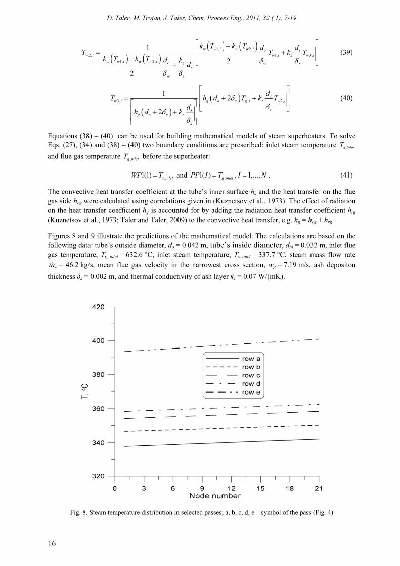
Figures 8 and 9 illustrate the predictions of the mathematical model. The calculations are based on the following data: tube’s outside diameter, do = 0.042 m, tube’s inside diameter, din = 0.032 m, inlet flue gas temperature, Tg ,inlet = 632.6 °C, inlet steam temperature, Ts, inlet = 337.7 °C, steam mass flow rate

sm& = 46.2 kg/s, mean flue gas velocity in the narrowest cross section, wg = 7.19 m/s, ash depositon thickness δz = 0.002 m, and thermal conductivity of ash layer kz = 0.07 W/(mK).

Fig. 8. Steam temperature distribution in selected passes; a, b, c, d, e – symbol of the pass (Fig. 4)


17

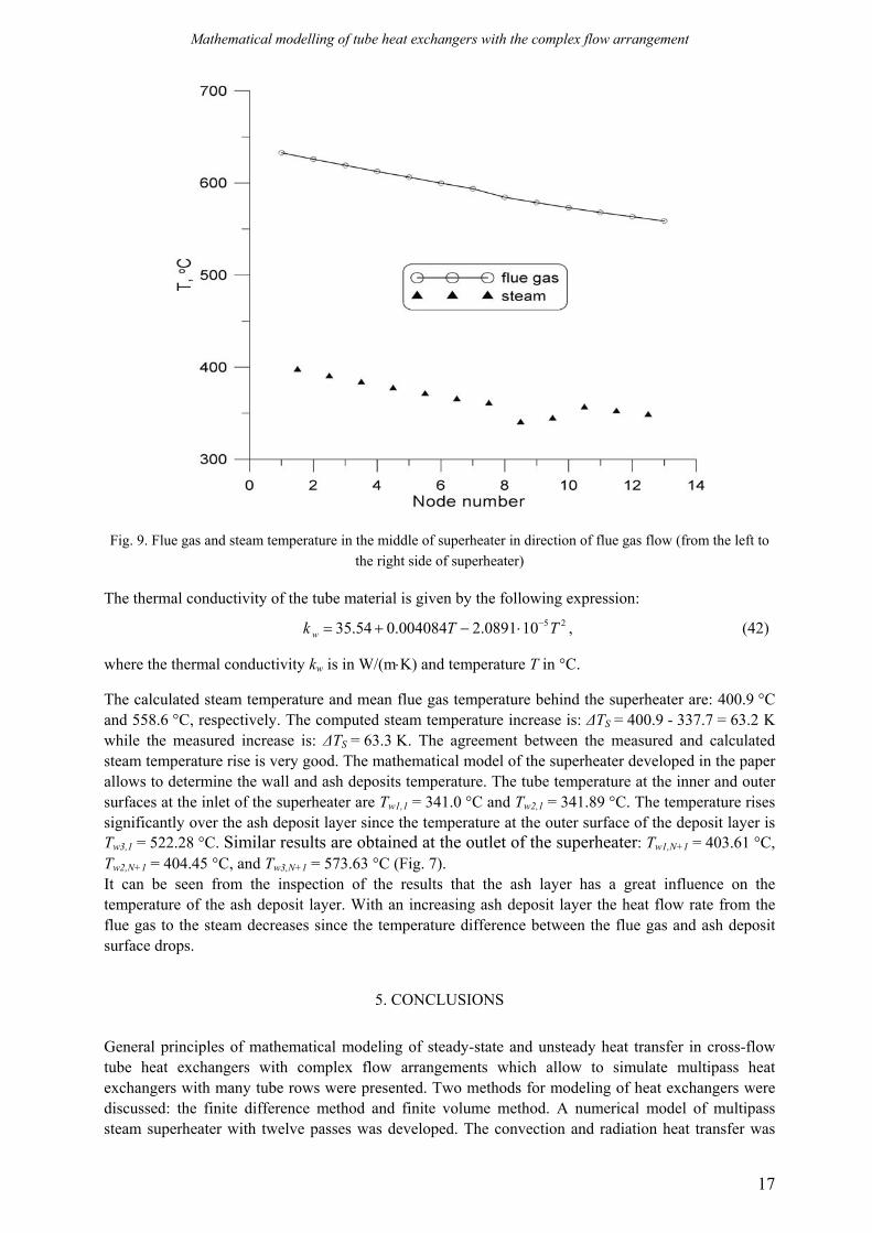
Fig. 9. Flue gas and steam temperature in the middle of superheater in direction of flue gas flow (from the left to the right side of superheater)

The thermal conductivity of the tube material is given by the following expression:

5 235.54 0.004084 2.0891 10wk T T−= + − ⋅ , (42)

where the thermal conductivity kw is in W/(m⋅K) and temperature T in °C.

The calculated steam temperature and mean flue gas temperature behind the superheater are: 400.9 °C and 558.6 °C, respectively. The computed steam temperature increase is: ΔTS = 400.9 - 337.7 = 63.2 K while the measured increase is: ΔTS = 63.3 K. The agreement between the measured and calculated steam temperature rise is very good. The mathematical model of the superheater developed in the paper allows to determine the wall and ash deposits temperature. The tube temperature at the inner and outer surfaces at the inlet of the superheater are Tw1,1 = 341.0 °C and Tw2,1 = 341.89 °C. The temperature rises significantly over the ash deposit layer since the temperature at the outer surface of the deposit layer is Tw3,1 = 522.28 °C. Similar results are obtained at the outlet of the superheater: Tw1,N+1 = 403.61 °C, Tw2,N+1 = 404.45 °C, and Tw3,N+1 = 573.63 °C (Fig. 7). It can be seen from the inspection of the results that the ash layer has a great influence on the temperature of the ash deposit layer. With an increasing ash deposit layer the heat flow rate from the flue gas to the steam decreases since the temperature difference between the flue gas and ash deposit surface drops.

5. CONCLUSIONS

General principles of mathematical modeling of steady-state and unsteady heat transfer in cross-flow tube heat exchangers with complex flow arrangements which allow to simulate multipass heat exchangers with many tube rows were presented. Two methods for modeling of heat exchangers were discussed: the finite difference method and finite volume method. A numerical model of multipass steam superheater with twelve passes was developed. The convection and radiation heat transfer was


18

accounted for on the flue gas side. In addition, the deposit layer was assumed to cover the outer surface of the tubes. The calculation results were compared with the experimental data. The computed steam temperature increase over the entire superheater corresponds very well with the measured steam temperature rise. The developed modeling technique can especially be used for modeling tube heat exchangers when detail information on the tube wall temperature distribution is needed.

SYMBOLS

A area, m2 inA , oA inside and outside cross section area of the tube, m2

c specific heat, J/kgK c mean specific heat, J/kgK

pc specific heat at constant pressure, J/kgK

FT correction factor for a particular flow arrangement, h heat transfer coefficient, W/(m2K) k thermal conductivity, W/(mK)

xL tube length in the heat exchanger, m m mass, kg m& mass flow rate, kg/s Q& heat flow rate, W r radius, m s1 pitch of tubes in plane perpendicular to flow (height of fin), m s2 pitch of tubes in direction of flow, m t time, s T temperature, °C

'2T , ''

2T gas temperature before and after tube row, °C U perimeter, m UA overall heat transfer coefficient, W/m2K Uin, Uo inner and outer perimeter of the oval tube, respectively, m w fluid velocity, m/s x, y, z Cartesian coordinates x+ = x/L dimensionless coordinate y+ = y/s2 dimensionless coordinate

Greek symbols α=k/(cρ) thermal diffusivity, m2/s

gmΔ & flue gas mass flow rate through the control volume , kg/s, TΔ temperature difference, K xΔ , yΔ control volume size in x and y direction, m

Δx+=1/N dimensionless control volume size δ thickness, m, ρ density, kg/m3 τ time constant, s

subscripts g flue gas lm logarithmic mean m mean r tube


19

s steam w wall in inner o outer 1 fluid flowing inside the tube 2 fluid flowing in perpendicular direction to tubes

REFERENCES

Hewitt G. F., Shires G. L., Bott T.R., 1994. Process heat transfer, CRC Press, Boca Raton. Kröger D. G., 1998. Air-cooled heat exchangers and cooling towers, Department of Mechanical Engineering,

University of Stellenbosch, Matieland, South Africa. Kuznetsov N. V., Mitor V.V., Dubovskij I.E., Karasina E.S. (Eds.), 1973. Standard methods of thermal design for

power boilers, Central Boiler and Turbine Institute, Energija, Moscow (in Russian). Rayaprolu K., 2009. Boilers for power and process, CRC Press, Boca Raton. Stultz S.C., Kitto J.B. (Eds.), 1992. Steam. Its generation and use, The Babcock & Wilcox Company, Fortieth

edition, Barberton, Ohio, USA. Taler D., 2009. Dynamics of tube heat exchangers, University of Science Publishing House (UNWD AGH),

Cracow (in Polish). Taler D., Taler J., 2009. Simplified analysis of radiation heat exchange in boiler superheaters. Heat Transf. Eng.,

30, 661-669, DOI: 10.1080/01457630802659953 Taler J., Trojan M., Taler D., 2009. Computer system for fouling assessment in coal-fired utility boilers. Arch.

Thermodyn., 30, 59–76.

ATHEMATICAL MODELLING OF TUBE HEAT...

Documents

Transcript of ATHEMATICAL MODELLING OF TUBE HEAT...