At a glance - Bureau of Infrastructure, Transport and ... · Australia’s commuting distance:...

<XX

> 73

Australia’s commuting distance: cities and regions

1

At a glance

• The aim of this Information Sheet is to generate estimates of average commuting distance for Australian capital cities, and other major cities and regions, based on the shortest path of road network distance.

• The estimates of 2011 average distance reflect recent evidence on commuting from home to a place of work at a range of spatial classifications or locality. The main interest is in understanding the patterns and average commuting distances under current land use and availability of transport infrastructure.

• On a place of residence basis, Australia’s average commuting distance was 15.6 km. • The average commuting distances for the rest of the state are generally higher than the

corresponding metropolitan areas. • The larger capital cities had relatively long commutes—Sydney’s average was 15.0 km,

Melbourne’s was 14.6 km, and Brisbane’s was 14.9 km, Perth’s was 14.9 km and Adelaide’s was 12.4 km. Smaller capital cities’ average commuting distance was shorter—Hobart’s was 11.5 km, Darwin was 12.3 km and the ACT was 11.5 km—reflecting the smaller urban footprint.

• The average commuting distance of residents of the major cities can be grouped into four ranges:

o 9–12 km: Townsville, Cairns, Launceston, Albury–Wodonga, Toowoomba and Canberra– Queanbeyan.

o 12–14 km: Bendigo, Darwin, Adelaide, Ballarat, Hobart o 14–15 km: Melbourne, Brisbane, Geelong, Perth, Sydney o 15–20 km: Newcastle-Maitland, Gold Coast–Tweed Heads, Sunshine Coast, Mackay and

Wollongong. • Average commuting distance by four BITRE regional classifications varied widely. Commuting

distances in Coastal Significant Urban Areas (SUAs) above 30,000 was 14.1 km and in Coastal SUAs with 10,000-30,000 population it was 16.5 km. Coastal country regions had a significantly higher average of 25.8 km, whilst Remote regions had an average of 31.2 km.

73

2

2

Context

BITRE’s studies (2011a, 2012, 2013a, 2013b) suggest that recent spatial changes in population, jobs and commuting flows in the capital cities largely reflect market forces, demography and people’s preferences as to where they live, work and do business. Government planning policies and infrastructure provision also play a role. State and territory governments believe that management of greenfield development, accommodation of population growth, and the transition to higher densities are most able to be influenced by planning (Productivity Commission 2011, p. xxiii).

BITRE (2012, 2013b) show that urban infill development played a more dominant role in accommodating Sydney’s population growth by concentrating new housing development within the existing urban footprint between 2001 and 2011. Sydney increased residential densities around the centres better than in either Melbourne or Perth from 2001 to 2006 (BITRE 2012: p. 11). Sydney’s employment is concentrated in the inner suburbs, while population is concentrated in the outer suburbs (BITRE 2012: pp. 3–4). Newman and Kenworthy (1996) demonstrate that such development has had significant impacts on urban travel patterns and the modal choice decisions. They further show that residential dispersal has encouraged more complex commuting and higher levels of car dependency.

This Information Sheet presents recent evidence on commuting distance from home to a place of work for Australian capital cities and regions. It is aimed at understanding the patterns and average commuting distances in major cities under the current land use and availability of transport infrastructure. This reflects the Australian Government’s focus on increasing productivity, including through efficient commuting. Integrated land use and transport infrastructure planning have some bearing on locational choices for households and businesses, and affect the commuting distance.

Measuring travel distances, including commuting distance, is a valuable task as these data are key descriptors of travel behaviour. They are also essential for deriving other statistics, for example, exposure to risks of accident; volume of externalities (congestion, emissions); and speed (Chalasani et al. 2005). Recent and accurate estimates of commuting distance can also contribute to understanding the interaction between work location and housing location choices.

There is a significant challenge in the efforts to integrate sustainable transport systems and land-use based planning strategies. The ability of integrated measures encompassing land-use and transport to promote efficiency gains in cities relies on gathering a range of evidence. This includes recent information on commuting distances and more broadly travel distances.

Previously BITRE produced four Research Reports which estimated commuting distance for four major capital cities in 2001 and 2006—Perth (BITRE 2010), Melbourne (BITRE 2011a), Sydney (BITRE 2012) and Brisbane (BITRE 2013a). These reports were based on the ABS Census Population and Housing—Journey to Work (JTW) 2001 and 2006 data in the previous Australian Standard Geographic Classification (ASGC 2006). BITRE also used the State’s specific estimates of commuting distance between origin and destination pairs based on road networks. A comparative cities report was subsequently added (BITRE 2013b), which included some ABS Census 2011 data, but did not include road commuting distance estimates for 2011.

Approach of the study

Aims The main aim of this Information Sheet is to generate estimates of average commuting distance for Australian capital cities. Estimates of average commuting distance will also be presented for other spatial classification including other major cities and regions in Australia.

The average distance presented here represents road network distance based on ArcGIS Network Analysis—weighted according to the latest census counts of commuters between Statistical Area 2 (SA2) origin-destination pairs. These were then aggregated to the Statistical Area 4 (SA4), Greater Capital City Statistical Area (GCCSA) and other localities scale.

73

3

3

This study examines the patterns of movement to increase understanding of comparative journey to work within and across cities and localities in Australia. Spatial distribution of commuting patterns by average distance is also illustrated in maps.

Key questions Most people in Australia travel to work by private motor vehicle, although some use combinations of car, public transport and walking. Of the 8.7 million people working on Census day 2011, 6.8 million or 78 per cent commuted from home to their place of work by private motor vehicle. About 12 per cent took public transport, 5 per cent rode a bicycle or walked, and 5 per cent worked at home.

A strong preference for commuting by motor vehicles arises in part from the accessibility, flexibility and convenience they provide. In addition to commuting, many workers also use their cars for other functions, including, transporting children to and from school, visiting elderly relatives and shopping. At times, motor vehicles are the only transport option as some workplaces are hardly accessible by public transport particularly in regional areas (ABS 2009).

As a high proportion of commuters travel by motor vehicle, this Information Sheet concerns commuting distance through the road network. Additional 3 per cent of commuting in Australia was by bus and 6 per cent use active transport,1 which also relied on the road network. Figure 1 shows the mode share of commuting in the capital cities and Australia in 2011. The shares of motor vehicle in journey to work by capital cities range between 71 per cent in Sydney and 83 per cent each in Adelaide and Darwin.

Figure 1Mode share of Journey to Work, capital cities and Australia, 2011

Source: BITRE analysis of the Australian Bureau of Statistics 2011Census of Population and Housing, journey to work data.

Three key questions arise:

• What were the average commuting distances in Australia’s cities and regions in 2011? • Which areas had a concentration of people commuting long distance? • Are commuting distances trending upwards over time?

Despite the flexibility offered by motor vehicles, there are economic and social costs of commuting. These include traffic congestion at peak hours, which puts pressures on road infrastructure and increases travel time for other commuters.

1 Active transport is travel which focuses on physical activity (walking and cycling).

73

4

4

Scope, data and method

Scope The scope of this Information Sheet is national—all employed persons aged 15 year and over, whose usual residence is defined in a locality, with commuting distances less than 250 km are included.2 Those with no fixed address or an undefined address as their place of residence or place of work are unable to be geocoded using a Geographic Information System (GIS) process and are excluded from the analysis. The main focus of the study is on Greater Capital City Statistical Areas (GCCSA) in Australia. Estimates for other major cities,3 coastal and other inland regions are also presented.

Capital cities accommodate a large share of Australia’s population and jobs. They particularly experience pressures on transport infrastructure. Analysis of smaller scales of geography within some larger cities enables an insight into the functions of different parts of a city. An analysis of the rest of the state/territory, as well as a summary classification such as coastal and inland regions, is also included.

Data There are two key data sources. For example to calculate the average commuting distance for Sydney GCCSA residents, we need information on the number of people commuting from an SA2 residence to any SA2 work location in Australia. In practice many of these SA2 pairs—such as commuting to SA2 of work in faraway states—will have zero values, reflecting no commuting. For example there were no commuters from an SA2 of Surry Hills residence in Sydney to an SA2 of Derby–West Kimberley work place in Western Australia. The average distance is the total commuting distance for all commuters living in the statistical region divided by the number of resident commuters. The data sources required are:

• Count of persons commuting from place of residence to place of work from the ABS Census of Population and Housing: Journey to Work (JTW) data 2011 by SA2 (Australian Statistical Geographic Standard/ ASGS 2011). This data is required for assigning weight in the distance calculation.

• Geocoded road network data—a GIS based road network database is used, namely the NAVTEC (2014 update) data underlying ESRI ArcGIS.

The scale of analysis at a small-area level is by SA2, that is commuting between SA2 of residence (population-weighted centroid) and SA2 of work (jobs-weighted centroid). Sensitivity testing was done to determine the small area level of analysis and is provided in the appendix.

Method A GIS tool is used to estimate commuting distance between each origin SA2 (place of residence) and destination SA2 (place of work) by road network, using the shortest-path distance. Distance is calculated between the population weighted centroid of the origin SA2 and the jobs-weighted centroid of the destination SA2. More specifically the GIS identifies the point along the road network which is closest to each centroid, and calculates the shortest road distance between both points

Schultes (2008) shows that a road network can be represented as a graph, which is a collection of nodes (junctions) and edges (road segments) where each edge connects two nodes. Each edge is assigned a weight, which is the length of the road. The computation of shortest paths between two nodes is assumed point-to-point—such as computing the shortest-path length from a given source node to a given target node (ibid). Map 1 provides an example of a shortest path distance between points—A and B.

In reality, commuters face several options and decide a path that will suit them in a particular situation and time. The assumption is often that that they take the lowest-cost path. This paper is however concerned with the shortest path. In this way, the average distance estimates presented in many cases can be thought of as providing a lower bound of the commuting distance by the road network.

2 The distance of up to 250 km commute is considered likely for daily commute. See also sensitivity testing in the appendix. 3 Major cities are based on Significant Urban Areas with population greater than 85,000.

73

5

5

The key component of this Information Sheet is the analysis of the average distance travelled to work by residents of a locality. The analysis is based on residents who work in a locality who commute by road up to a maximum distance of 250 km.4 Lengthy commutes are addressed in another BITRE study (forthcoming).

The number of commuters is available from the ABS Census of Population and Housing data for 2011 which can be disaggregated by Statistical Area 2 (SA2) of usual residence and SA2 of work. This data was downloaded from the ABS using TableBuilderPro to form a national matrix of commuting flows between SA2 origin-destination pairs in 2011.

Map 1 Shortest Path Distance

Source:

ESRI-ArcGIS,http://help.arcgis.com/en/arcgisdesktop/10.0/help/index.html#

//004700000001000000

Commuting distance in cities: review of literature

The shape and nature of large cities have changed. Suburbanisation and urban sprawl, along with the formation of urban networks, has led to an increase of commuting flows, shaping the development of transport infrastructure and inter-firm linkages and allowing for the pooling of a self-contained labour market’ (OECD 2006: p.13).

De Goei et al. (2010) stated that contemporary literature on changing urban systems argues that the traditional central place conceptualisation needs to be updated and developed. One option is to develop a network view that emphasises the increasing criss-crossing pattern of interdependencies between spatial units. There is some evidence for a monocentric urban network development at the intra-urban or local level, and a decentralisation of the system at the inter-urban or regional level (ibid.).

‘The concept of the monocentric city involves a central unit, the central business district, surrounded by a circular residential area whereby land is allocated according to its most profitable use. The general idea of the monocentric city is that most economic activities are based in the urban core, whereas suburbs only fulfil a residential function. Hence, the relationship between the urban core and its suburbs in the monocentric model is hierarchical–nodal or centralized in the sense that most commuting flows are directed from the suburban areas towards the central cities’ (De Goei et al.: p. 1152). At the same time, there is evidence of cities with multiple centres or polycentric cities (ibid.). A question arises whether polycentric cities mean decentralisation and alignment of jobs and population.

Burger et al. (2014) suggest that urban networks are multi-dimension phenomena and that spatial interaction within and between cities can take many different forms. The spatial organisation of each of these functional linkages—including commuting and inter-firm trade—is not necessarily the same. Therefore, a region can appear to be polycentric and spatially integrated based on the analysis of one type of functional linkage but monocentric and loosely connected based on the analysis of another type of functional linkage (ibid.). This study explores one functional linkage in the form of commuting flow and patterns of the journey to work in major cities and the rest of state in Australia.

4 The distance of up to 250 km commute is considered likely for daily commute. See also sensitivity testing in the appendix.

73

6

6

Cervero (1995) shows that an argument for decentralisation of jobs simply aimed for achieving jobs-housing balance is missing some points because ‘jobs-housing balance has both quantitative and qualitative dimensions—balance requires a concordance of worker earnings and local housing prices, not just numerical parity’ (Cervero 1995: p. 336). How well our cities are functioning does not depend solely on planning. ‘Good planning can create the environment for efficient and effective cities but the outcome is also dependent on the market, governments’ investment in infrastructure, and other government policies and actions (such as immigration policy and delivery of services)’ (Productivity Commission 2011, p. xxiii).

Different urban spatial structures encourage efficient modes of travel. Newman and Kenworthy (1989, 1999) show a positive relationship between transport energy consumption and distance from Central Business District (CBD) and a negative relationship with the density of cities. The less dense the city and the further average distance from home to work, the more transport energy consumption. Planners have sought particularly to increase public transport mode share and reduce car use through urban land use planning as shown in Table 1. Nevertheless more consistent evidence of the effectiveness of such initiatives is required (Humphreys and Ahem 2013) and in particular to show direct causality.

Table 1 Types of Urban spatial structure

Type of city structure

Spatial layout Travel characteristics

Monocentric It has a declining density gradient from the city centre outwards with centralised economic activity

Strong radial movement that favours public transport provision with limited need for private car. E.g. Dublin

Mono-Polycentric The CBD remains the main area of economic activity but increasing decentralisation of jobs has weakened the dominance of CBD

Strong radial travel to CBD and high public transport use but suburban travel mainly by private car. E.g. London

Polycentric (urban village or activity centre based)

Intra-urban patterns of clustering of population and economic activity consisted of independent multiple centres

Majority live near work and travel locally with high share of sustainable travel modes. E.g. Seoul

Polycentric (sprawl)

Sub-centres present but no dominant centre with dispersed employment and services

Each sub-centre generates trips from dispersed areas of the city. E.g. Perth

Source: Adjusted from Humphreys and Ahem 2013.

There has been conflicting evidence emerging from studies of the impacts of polycentric-like structures and employment decentralisation on commuting patterns. For example Gordon et al. (1991) demonstrates that polycentric metropolitan structures are favourable to short commutes. Conversely, Song (1992) shows that when applied to United States metropolitan areas, polycentric structures require longer commute relative to a monocentric model. Nevertheless many studies agree that travel times are shorter for workers heading to suburban centres than to CBDs, ‘confirming that those travelling in outlying areas average higher speeds’ (Cervero 1995: p. 336).

Wheaton’s study (2004) on commuting, congestion and employment dispersal in American cities displays that there is a difference in average commuting distance between centralised jobs and jobs in dispersed locations. Centralised jobs can result in agglomeration benefit and may involve higher wages and longer commutes, while jobs in dispersed locations tend to involve lower wages and shorter commuting distances. Greater traffic congestion, particularly for inward commuting to the CBD in peak hour in certain industries seems to lead to employment decentralisation (ibid.).

Australia’s major capital cities have experienced increases in knowledge intensive industries that are often concentrated in central areas in order to capture agglomeration benefits (BITRE 2013b, Rawnsley et al. 2011). Brotchie et al. (1995) completed a study on commuting trips in major Australian capitals by industries and occupations showing that most central job locations are advanced producer services industries,5 and in occupation such as managers and professionals, para professionals and other higher income earners. These with most central jobs also had more central home locations. The most dispersed job locations are for extractive and transformative industries, for example manufacturing industry, including occupations such as machinery operators and trade persons, who relatively had less income than professionals (Brotchie et. al.1995: p. 40).

5 Advanced producer service firms include accountancy, advertising, architecture, finance and law.

73

7

7

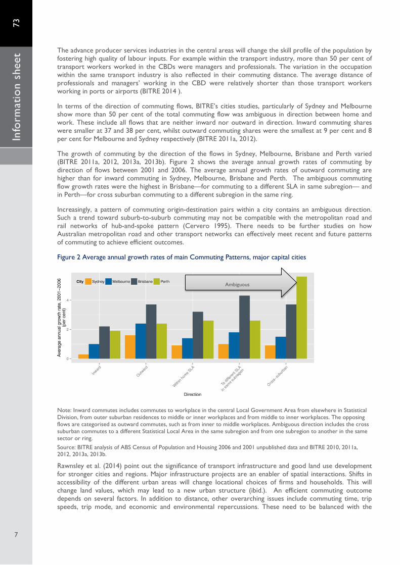
The advance producer services industries in the central areas will change the skill profile of the population by fostering high quality of labour inputs. For example within the transport industry, more than 50 per cent of transport workers worked in the CBDs were managers and professionals. The variation in the occupation within the same transport industry is also reflected in their commuting distance. The average distance of professionals and managers’ working in the CBD were relatively shorter than those transport workers working in ports or airports (BITRE 2014 ).

In terms of the direction of commuting flows, BITRE’s cities studies, particularly of Sydney and Melbourne show more than 50 per cent of the total commuting flow was ambiguous in direction between home and work. These include all flows that are neither inward nor outward in direction. Inward commuting shares were smaller at 37 and 38 per cent, whilst outward commuting shares were the smallest at 9 per cent and 8 per cent for Melbourne and Sydney respectively (BITRE 2011a, 2012).

The growth of commuting by the direction of the flows in Sydney, Melbourne, Brisbane and Perth varied (BITRE 2011a, 2012, 2013a, 2013b). Figure 2 shows the average annual growth rates of commuting by direction of flows between 2001 and 2006. The average annual growth rates of outward commuting are higher than for inward commuting in Sydney, Melbourne, Brisbane and Perth. The ambiguous commuting flow growth rates were the highest in Brisbane—for commuting to a different SLA in same subregion— and in Perth—for cross suburban commuting to a different subregion in the same ring.

Increasingly, a pattern of commuting origin-destination pairs within a city contains an ambiguous direction. Such a trend toward suburb-to-suburb commuting may not be compatible with the metropolitan road and rail networks of hub-and-spoke pattern (Cervero 1995). There needs to be further studies on how Australian metropolitan road and other transport networks can effectively meet recent and future patterns of commuting to achieve efficient outcomes.

Figure 2 Average annual growth rates of main Commuting Patterns, major capital cities

Note: Inward commutes includes commutes to workplace in the central Local Government Area from elsewhere in Statistical Division, from outer suburban residences to middle or inner workplaces and from middle to inner workplaces. The opposing flows are categorised as outward commutes, such as from inner to middle workplaces. Ambiguous direction includes the cross suburban commutes to a different Statistical Local Area in the same subregion and from one subregion to another in the same sector or ring. Source: BITRE analysis of ABS Census of Population and Housing 2006 and 2001 unpublished data and BITRE 2010, 2011a, 2012, 2013a, 2013b.

Rawnsley et al. (2014) point out the significance of transport infrastructure and good land use development for stronger cities and regions. Major infrastructure projects are an enabler of spatial interactions. Shifts in accessibility of the different urban areas will change locational choices of firms and households. This will change land values, which may lead to a new urban structure (ibid.). An efficient commuting outcome depends on several factors. In addition to distance, other overarching issues include commuting time, trip speeds, trip mode, and economic and environmental repercussions. These need to be balanced with the

Ambiguous

73

8

8

public policy propositions of urban development to achieve the multi-dimensional objective of efficient outcome (Cervero 1995).

The ambiguity in the literature about the influence of urban structure on commuting (Humphreys and Ahern 2013) reflects other factors—residential-self-selection, skills/qualifications, amenity, income and the presence of transport infrastructure—and how these affect commuting. Kitamura et al. (1997) examined the effects of land use and attitudinal characteristics on travel behaviour in San Francisco. They found that attitudes to travel are more strongly associated with commuting patterns than are land use characteristics.

Many economic models and policy analyses rely on the belief that land-use patterns strongly affect commuting. Yet the empirical evidence is inconsistent (Giuliano and Small 1993: p. 1485). Public policy has often focused on the relationship between commuting distance and the locational patterns of jobs and housing. Increased congestion has been linked to mismatch between jobs and housing, where housing prices in the area are unsuitable for local workers, making inter-area commutes necessary. Some of the evidence suggests ‘that commuting distance and time are not very sensitive to variation in urban structure’ and there are behavioural factors that may be missing in the analysis but need to be taken into account in the results (ibid.: p. 1486).

The present scale of land use patterns in our capital cities is relatively large. This means that only a small share of trips include a commuting trip short enough for walking. The dispersed nature of our cities is such that only small share can be served by public transport, but mass rail transit allows some expansion and motor vehicles have allowed a further dispersal from the centre of the cities (Brotchie et al. 1995). The BITRE’s cities studies show that the share of central city jobs in the major capital Australian cities is approximately one-fifth. This includes jobs in company headquarters and a range of advanced producers and specialist services, for example as legal, finance, insurance, advertising and travel. Generally, the central city labour market extends across metropolitan areas and beyond and also to large suburban centres. Jobs usually outnumber residences in the city centrals, whilst housing outnumbers jobs in the suburbs (BITRE 2011a, 2012, 2013a, 2013b; Brotchie et al. 1995).

Cervero (1995), following Newman and Kenworthy (1989), suggests that there is a link between high motor vehicle mode share to dispersal of jobs and to lower residential densities. While jobs-housing imbalances have been suggested as one of the reasons for longer commuting distance, others have suggested that there are other factors besides job access influencing locational choice of residence and hence commuting distance. A range of other factors such as quality of schools, neighbourhood’s amenities, mixes of community services and familial ties are found to be significant factors (Cervero 1995).

Average commuting distance

Capital cities and the rest of state Australian capital cities and the rest of the state/territory differ in their geography and size, their land-use and transport conditions and their demographic and socio-economic conditions. This is shown in the variations in their average commuting distances.

The analysis of commuting distance presented here relates to the shortest path by road networks distance using GIS, based on the SA2 origin and destination of commuting. Figure 3 shows that in 2011, based on a place of residence, Australia’s average commuting distance was15.6 km. In the larger capital cities—Sydney’s average was 15.0 km, Melbourne’s was 14.6 km, and Brisbane’s was 14.9 km, Adelaide’s was 12.4 km and Perth’s was 14.9 km. Smaller capital cities’ average distance was shorter—Hobart’s was11.5 km, Darwin was 12.3 km and the ACT was 11.5 km—reflecting the smaller urban footprint of these areas. The average commuting distance figures for the rest of the state are generally higher than the corresponding metropolitan areas, except for Darwin and the rest of the Northern Territory (NT). The result for the rest of NT implies that workers in the rest of this state commuted mainly locally, with average commuting distance of 8.6 km.

73

9

9

Figure 3 Average Commuting Distance by place residence in capital cities and the rest of the state/territory, 2011

Source: BITRE analysis of ABS Census of Population and Housing 2011, origin-destination commuting flows extracted from Table BuilderPro and road network analysis from ArcGIS

Major cities Major cities here are defined as all capital cities with concentrations of urban development based on Significant Urban Areas (SUAs) and with populations of more than 85,000. The ABS characterises an SUA as either a single urban centre or a cluster of related urban centres with a core urban population greater than 10,000.

Figure 4 shows the Estimated Resident Population (ERP) of the major cities, which includes the capital cities and 13 other cities. In 2014 the population for GCCSAs ranged between 140,400 in Darwin and 4,840,600 in Sydney. The population of the rest of the major cities varied widely. Significant Urban Areas in Ballarat, Bendigo, Albury-Wodonga, Launceston and Mackay had between 85,000 and 100,000 residents. The rest of the SUAs had populations over 100,000 with Gold-Coast-Tweed Heads notably reaching 614,400 people in 2014 (ABS 2015).

The average commuting distance of residents of the major cities can be grouped into four ranges:

• 9–12 km: Townsville, Cairns, Launceston, Albury–Wodonga, Toowoomba and Canberra– Queanbeyan.

• 12–14 km: Bendigo, Darwin, Adelaide, Ballarat, and Hobart • 14–15 km: Melbourne, Brisbane, Geelong, Perth, and Sydney • 15–20 km: Newcastle-Maitland, Gold Coast–Tweed Heads, Sunshine Coast, Mackay and

Wollongong.

Figure 5 shows major cities average commuting distance by place of residence. Places of residence such as Wollongong, Gold Coast–Tweed Heads and Sunshine Coast—those are close to a capital city—tend to have relatively high average commuting distance (19.7 km, 16.9 km and 17.1 km respectively). For example, 13 per cent of residents of Wollongong commuted more than 50 km. Similarly, some residents of Miami in Gold Coast and Marcoola in Sunshine Coast commuted up to 70 km to work in different areas in Brisbane.

On a place of residence basis, the main capital cities—Sydney, Melbourne, Brisbane, Perth and Adelaide—show a similar pattern in the distribution of commuting distance (Figure 6). These major cities had around one-quarter of commuters with a distance of less than 5 km, whilst Darwin and Hobart had almost one-third of commuters with a journey to work of less than 5 km in 2011.

73

10

10

Figure 4 Estimated Resident Population, by major cities, 2014

Note: Capital cities here use the GCCSA boundary. The ACT is included for completeness of presentation of capital cities and the rest of the major cities include the SUA of Canberra- Queanbeyan.

Source: ABS Cat. No. 3218.0 Regional Population Growth Australia, March 2015 release.

Figure 5 Average commuting distances by place of residence, Major cities, 2011

Source: BITRE analysis of ABS Census of Population and Housing 2011, origin-destination commuting flows extracted from Table BuilderPro and road network analysis from ArcGIS.

Figure 6 further shows that around one-half of commuters in all capital cities had a commuting distance of less than 10 km. In Sydney, Melbourne, Brisbane, Adelaide and Perth just over 16 per cent of commuters had commuting distance between 10 and 15 km. A further 12 per cent of the commuters travelled between 15 and 20 km. The rest of the commuters in Sydney, Melbourne, Brisbane, and Perth—around a quarter in each city—commuted more than 20 km.

Figure 6 Distribution of commuting distance for residents of capital cities and Australia, 2011


73

11

11

Most journeys to work in major cities are by car, criss-crossing the inner, middle, and outer suburbs. Some areas have more jobs than workers and therefore receive a net inflow of commuters, whilst other areas have fewer jobs than workers and thus experience a net outflow of commuters (Forster 1995). The patterns of commuting distance in each city are combinations of all employed residents who commute either in the local area, across suburbs or to other areas—including the city centrals.

On examining the share of commuters by distance range in the capital cities—particularly the two shortest less than 5 km and between 5 and 10 km; and the two longest—between 30 and 50 km, and greater than 50 km ranges of commuting distance—Sydney, Melbourne, Brisbane, Perth, and to a certain extent Adelaide exhibited a similar pattern (Figure 7a). In most cases, the share of commuting less than 5 km was the largest, followed by the share of commuting between 5 and 10 km. The share of commuting distance of more than 50 km was the smallest.

The rest of the major cities showed a similar general pattern but with a slightly different distribution. The two shortest commuting distances still dominated. However the largest distance range (over 50 km) did not necessarily have the smallest share of commuters (Figure 7b).

For example, Toowoomba, Ballarat, Bendigo, and Albury-Wodonga had significant shares—approximately 80 per cent—of residents commuting less than 10 km. In contrast, cities such as Wollongong, Geelong, and Gold Coast-Tweed Heads had up to 13 per cent commuting more than 50 km. For instance, up to 13 per cent of Wollongong residents commuted to the Sydney area, whilst almost 50 per cent commuted less than 10 km. Similarly, up to 10 per cent of Geelong residents typically commuted more than 50 km to a place of work in Melbourne, whilst around two-thirds commuted less than 10 km.

Figure 7 Share of resident commuters by distance, major cities, 2011

a. Capital cities

b. The rest of the major cities


73

12

12

Coastal, inland and remote regions Adding an extra dimension to locational choice is a preference towards ‘amenity’. The population of many of Australia’s coastal cities is increasing at a faster rate than that of Australia overall (BITRE 2011b). Growing coastal country regions are often characterised by close proximity to a large coastal city or a capital city. The growth from sea change migration often involves older people moving from capital cities as they ease into retirement. Attractive lifestyle and high levels of amenities located in coastal cities—such as Gold Coast, Sunshine Coast, Hervey Bay and Cairns—are a factor in Australia’s long standing preference for coastal living (ibid.; p.40).

To capture a comparative amenity aspect of residential areas, an approach based on BITRE study (2011b) is used to classify regions. This analysis illuminates relationships between residential preference, choice of a work place and commuting impacts. This BITRE classification of region was updated using SA2 to cover four major region types, namely, Capital cities (GCCSAs), Coastal, Remote and Inland regions.

Coastal regions are characterised by one SA2 centre point that is within 50 km of the coast. Remote regions in this case typically coincide with the remote and very remote category of the ABS remoteness structure. Inland regions cover the remaining area (BITRE 2011b).

By including population ranges related to SUAs, this section employs the BITRE region type that can be further grouped as follows (BITRE 2011b):

1. Capital cities 2. Coastal a) SUAs with population above 30,000 b) SUAs with population between 10,000 and 30,000 c) Non-SUAs (or coastal country) 3. Inland a) SUAs above 30,000 b) SUAs with population between 10,000 and 30,000 c) Non-SUAs (or inland country) 4. Remote

The estimated resident population (ERP) of Australia’s coastal regions in 2013 was 5.3 million. Around 62 per cent of the ERP was in the Coastal SUAs with more than 30,000 people, 12 per cent in the SUAs with 10,000–30,000 people and 26 per cent was in coastal country regions.

People choose where to live based not only on employment and industry but often also on amenity at a particular stage of life. For example, a mature age person easing into retirement might choose to settle in a coastal town with preferable amenities. He or she may be prepared to commute longer distances a few days each week. Such a case has provided a functional niche for Australian coastal cities to offer support industries catering to the needs of the local population, in addition to their traditional industries (BITRE 2014b: p. 265).

Figure 8 shows averages commuting distance by place of residence of BITRE region type. Coastal SUAs had average distances of 14.1 km and 16.5 km for SUAs above 30,000 population and SUAs with 10,000–30,000 population respectively. The Coastal SUAs contained 17 per cent of overall ERP in Australia in 2013

The Coastal country regions had a significantly higher average of 25.8 km, the second highest average distance after the Remote regions (31.2 km). The Coastal country (Non-SUAs) contained 6 per cent of overall ERP. For example many residents of Huskisson–Vincentia SA2 commuted to North Nowra–Bomaderry SA2 and SUA (25.8 km) in NSW. Some residents of the Northern Beaches SA2 worked in Condon-Rasmussen SA2 (26.9 km) within the Townsville SUA in Queensland.

In contrast, the Inland SUAs had relatively lower average commuting distances between 10.4 km and 12.8 km, implying residents were more likely to commute locally. The Inland SUAs contained 6 per cent of overall ERP.

For the remainder of the Inland Non-SUA regions, the average commuting distance of the Inland country region (23.8 km) were larger than their corresponding SUAs’ averages. The dispersal of population within the Inland country as well as in the Remote regions means that they typically commute to the closest SUA. This was one of the factors which contribute to the higher average commuting distances. For example, many

73

13

13

residents live and work locally. Others, such as some residents of Longford SA2 commuted to the closest SUA work location in Launceston (18.2 km). Moreover some residents of Clare SA2 worked in Gilbert Valley SA2—both of which are country regions in South Australia (24.2 km).

Remote regions such as Balonne in Queensland typically cover a large land area (31,106 square km). Some residents who worked and lived in Balonne may have even higher than the average commuting distance of the Remote region (31.2 km) due to the sheer size of the vast region.

Figure 8 Average commuting distances of residents by BITRE region type, 2011

Note: Care needs to be exercised when examining relatively large Remote and Non-SUA areas because the approximation of the centre points of jobs and residential areas may introduce inaccuracy of the average distance.

Source: BITRE analysis of ABS Census of Population and Housing 2011, origin-destination commuting flows extracted from Table BuilderPro and road network analysis from ArcGIS; and also coastal classifications from BITRE 2011b.

To appreciate the higher average commuting distances in both country (Non-SUAs) Coastal and Inland regions as well as in the Remote region, Figure 9 shows the distribution of shares of commuters, by their average commuting distance, by the region type. The share of commuting distance over 50 km is relatively high for the Remote region (22 per cent), Inland Non-SUAs (14 per cent) and Coastal Non-SUAs (12 per cent). In contrast, Capital cities had the smallest share (2 per cent) in the highest average commuting distance range.

Figure 9 Shares of commuters by the average commuting distance by BITRE region type, 2011

Note: Care needs to be exercised when examining relatively large Remote and Non-SUA areas because of the approximation of the centres of jobs and residential areas may introduce inaccuracy of the average distance.

Source: BITRE analysis of ABS Census of Population and Housing 2011, origin-destination commuting flows extracted from Table BuilderPro and road network analysis from ArcGIS; and also coastal classifications from BITRE 2011b.

73

14

14

BOX 1 Case Study of the Grampians in North West Subregion, Victoria

A case study of the Grampians Statistical Area (SA3)6 in the North West Subregion in Victoria has been selected to illustrate patterns of commuting by residents of inland country areas. Although this case study of the Grampians is based on a single SA3, it illustrates relative commuting distances in regional areas. The case study was also informed by research on the ways workers used commuting rather than migration to address issues of labour mobility—particularly in facing the issue of an industry shock in parts of the Grampians (McKenzie and Frieden 2010).

The Grampians consists of nine SA2s namely Ararat, Ararat Region, Horsham, Horsham Region, Nhill Region, St Arnaud, Stawell, West Wimmera and Yarriambiack. The Grampians as a whole had a total population of 58,920 in 2014. The regional centres of Ararat, Horsham and Stawell have populations of between 8,000 and 16,330 and a significant employment base. They had a range of health services, education facilities and commercial precincts. The rest of the towns in the Grampians have a moderate population and housing base with retail and employment areas and access to education and health services. Some of these towns have employment links with regional centres or other higher order settlements nearby (Victoria Department of Transport, Planning and Local Infrastructure 2014).

All of the SA2s in the Grampians SA3—except Horsham—are Inland country Non-SUAs. Horsham SUA is the largest employment centre in the Grampians. Horsham is a regional centre with a hinterland of small rural towns which have experienced demographic changes—particularly population decline and economic restructuring (Wilkinson and Butt 2013: p. 79). As shown in Table B.1, Horsham had the largest number of residents (16,330) and largest number of jobs (6,740). In contrast, West Wimmera had both the smallest population (2,690) and the lowest number of jobs (1,230).

In 2011 the Grampians had employment of 23,930. Agriculture, Forestry and Fishing was the largest employing industry (4,320). This was followed by Health Care and Social Assistance (3,830) and Retail Trade (2,660). The industry structure is shown in Figure B.1.

Figure B.1 Grampians SA3, Employment by industry, 2011

Source: BITRE analysis of ABS Census of Population and Housing 2011, Employment by Industry, Place of work data.

As shown in Table B.1, except for the three largest regional centres in the Grampians—Ararat, Horsham and Stawell—Agriculture was the major employing industry for all the SA2s, In Ararat, Horsham and Stawell Health Care and Social Assistance industry dominated as the top employing industry. These three regional centres also had the three smallest shares of employed residents who worked at home in 2011 Census (2.7 per cent, 3.5 per cent and 6.4 per cent respectively). Nevertheless as illustrated in Table B.1, Horsham, Ararat and Stawell also had the three shortest average commuting distances by SA2 of residence, at 7.3 km, 9.5 km and 10.0 km respectively.

6The Grampians here refers to the ABS Statistical Area 3 and it is not the same as the Victorian Government defined region of the Grampians. Similarly Ararat and the corresponding Ararat Region, and Horsham and the corresponding Horsham Region are each considered as a distinct Statistical Area 2.

73

15

15

Commuting in Horsham, Ararat and Stawell is two-way. The residents of these areas also commuted to the nearby small rural towns for work. In 2011, between 4 per cent and 6 per cent of these regional centres’ residents commuted outside of their home SA2. Such interactions around the regional centres enable smaller areas to extend their reach creating an economic network. Workers from outside areas commuting inward into the regional centres are subject to lack of jobs within their home areas. Those commuting outwards from the regional centres filled a void created from a lack of professionals residing in smaller towns (Wilkinson and Butt 2013: pp. 81-3).

Table B.1 Grampians Average commuting distance, Population, and Employment profile, 2011

SA2 name Average distance* (km)

Population 2014

Employment 2011

Share of Work at Home (per cent)

Largest Employing Industry

Ararat 9.5 8,070 3,000 2.7 Health Care and Social Assistance

Ararat Region 27.0 2,930 1,300 27.6 Agriculture Forestry Fishing

Horsham 7.3 16,330 6,740 3.5 Health Care Social Assistance

Horsham Region 17.8 3,390 1,610 20.9 Agriculture Forestry Fishing

Nhill Region 23.6 6,970 2,790 16.2 Agriculture Forestry Fishing

St Arnaud 15.3 3,520 1,420 13.7 Agriculture Forestry Fishing

Stawell 10.0 8,210 3,290 6.4 Health Care Social Assistance

West Wimmera 25.1 2,690 1,230 25.9 Agriculture Forestry Fishing

Yarriambiack 21.0 6,830 2,560 14.4 Agriculture Forestry Fishing

Grampians SA3 13.9 58,920 23,930 10.7 Agriculture Forestry Fishing

Note: *Average distance by Place of usual residence (PUR). Care needs to be exercised when examining relatively large Non-SUA areas because the approximation of the centre points of jobs and residential areas may introduce inaccuracy of the average distance.

Source: BITRE analysis of ABS Census of Population and Housing 2011, origin-destination commuting flows extracted from Table BuilderPro and road network analysis from ArcGIS and Employment by Industry by Place of work (rounded). ABS, Regional Population Growth, Cat. No 3218.0, March 2015.

The relatively large range of average commuting distances among the SA2s that make up the Grampians can be better represented spatially. Horsham, Ararat and Stawell had the shortest commuting distances as illustrated in the lightest shade range shown in Map B.1. Notably Horsham and Ararat SA2 cover the two smallest geographical areas. Horsham and Ararat had the two highest population numbers, as shown in the circles for the SA2s.

St Arnaud and Horsham Region followed next with averages commuting distances of 15.3 km and 17.8 km respectively. St Arnaud’s distribution of commuting distance in the two extreme ends of the distance range was typical of a regional area with Agriculture as the major employing industry. Most employed residents (84 per cent) in St Arnaud worked close to home—commuting less than 5 km. Around 16 per cent of the employed residents commuted more than 50 km. For example, they travelled to work in nearby areas such as Stawell, Buloke, Horsham or Bendigo (up to 106 km). Wilkinson and Butt’s (2013) study on Victoria’s regional commuting suggests that small towns located within the sphere of influence of the nearest regional centre have become part of its economic network. Commuting in this way has filled a gap in employment created by the economic and demographic trends in regional Australia.

Average commuting distances for the three larger geographic areas of Nhill, West Wimmera and Yarriambiack follow a similar pattern to St Arnaud. There are 5 Destination Zones (DZs) each in Nhill and Yarriambiack and 3 DZs in West Wimmera, which were used to estimate the centres of jobs. However because of the large areas and the limited destination zone disaggregation the approximation of the centre points of jobs and population are likely to be imprecise, thus care needs to be exercised when looking at these results.

Many farmers in regional Victoria have changed their location or their employment characteristics. ‘Off-farm income has become more important and some farmers have moved into towns where they and their families can access services and additional income sources more easily. In effect, they have become commuters—living in a town or regional city but travelling to their properties’ (McKenzie and Frieden 2010: p. 17).

73

16

16

Map 2 Average commuting distances, by SA2 of residence, and Population, 2011

Note: Care needs to be exercised when examining Non-SUA areas because of the large areas and the limited destination zone disaggregation, the approximation of the centre points of jobs and population are likely to be imprecise; thus care needs to be exercised when looking at these results.

Source: BITRE analysis of ABS Census of Population and Housing 2011, Journey to Work data and Network Analysis ArcGIS and ABS, Regional Population Growth, Cat. No. 3218.0

McKenzie (2012) investigated the impact of industry shocks on towns in regional Victoria. The study found that generally workers preferred to commute rather than relocate to access new work opportunities. She argues that the advantage of commuting over relocation was around social factors—the ability to remain in a home community with the accustomed support, security and identity to workers and their families (McKenzie 2012).

Stawell is a particular case of an industry shock. It is located on the far western edge of the goldfields of central Victoria, 235 km west of Melbourne and 130 km from Ballarat in Western Victoria. The local underground gold mine operated for 30 years employing approximately 350 people at its peak in the last decade. In 2012, the mine’s closure was announced due to increased costs and uncertainties on future profitability. In response to the impending closure, the opportunity to undertake fly-in fly-out (FIFO) or drive-in drive-out (DIDO) commuting to other mines in Australia was identified (McKenzie and Frieden 2010). This option of lengthy commuting allows many to work in the mining industry without uprooting families and social networks (Parliament of Australia 2013: p. 2). As important as this type of commuting is, it is beyond the scope of this Information Sheet which only considers commuting up to 250 km.

In 2011, the distribution of commuting in Stawell followed a regional pattern with the majority (86 per cent) commuting locally less than 5 km distance. Around 9 per cent of the residents commuted to Ararat, with an average commuting distance of 33 km. Approximately 5 per cent commuted more than 50 km, for example to Horsham, Wendouree-Miners Rest or Ballarat (up to 120 km).

The Grampians’ case study of regional commuting presented here reflects the regional mobility of labour. Such mobility is a mechanism for a flexible and efficient economic system where workers commute to areas of greatest employment and or wage level (Productivity Commission 2013: p. 1).

73

17

17

Average commuting distance in city subregions The majority of the Australia’s population—almost two-thirds—resides in the capital cities. This section examines the average commuting distance in subregions within the GCCSAs and highlights differences in commuting distance from subregions within a city.

Patterns of work travel reflect the outcomes of complex processes in deciding where to live and work. This section highlights some results of the concentration of the significantly longer and shorter than average commuting distances. It also shows such patterns across and within Australian cities.

The commuting patterns within cities seem to be enduring, with limited changes in certain parts of the cities. For example the distribution of places of work relative to residence seemed to remain relatively stable in Sydney. This is reflected by very small changes in self-containment rates—the share of employed residents who work in the home subregion (BITRE 2012: p. 274). ‘For urban policy, a high rate of travel self-containment indicates a set of land-use and transport conditions sufficient to satisfy much of local residents’ needs’. Similarly, other Australian cities have rarely significantly increased their self-containment (Yigitcanlar et al. 2007: p. 131). This implies relative stability in travel distance. In the main capital cities the basic density of jobs and residence continue to largely be in line with their established patterns (BITRE 2011a, 2012, 2013a, 2013b).

Map 1 illustrates the average commuting distance by subregion of residence (Statistical Area 4/SA4) in capital cities. There is a pattern of inner ring residents having the shortest average distance (7–10 km), followed by the middle ring residents (10–15 km). Outer ring residents have the highest average commuting distances (greater than 15 km).

In Sydney, three subregions of residence—City and Inner South, Eastern Suburbs, and Inner West— had the shortest average commuting distances. In the other main capital cities—the Melbourne Inner, Brisbane Inner City, Perth Inner and Adelaide West subregions—were the only one in each corresponding metropolitan with an average commuting distance of less than10 km. This is typically in the central part of the inner ring.

On a place of work basis, the inner ring or central subregions had relatively high average commuting distances. ‘An area’s ability to attract workers from further afield is related to its industry specialisation and the size of the employment agglomeration’ (BITRE 2013a: p. 266). Such areas often have an intense concentration of specific industries brought about by globalisation and deindustrialisation. This often indicates an advanced economy’s effective transition from sizeable manufacturing sector to advanced producer services with most people involved in information exchanges. Some prime areas are able to transition to the new knowledge economy, based on information services (Hall 2011).

The central areas in the main capital cities are in an advantaged position to host the knowledge-intensive businesses which place a premium on being near each other (Kelly and Donegan 2015: p. 35). Table 2 shows the average distance by subregion of work and the selected subregions’ share of employment in knowledge-intensive industries, and the three largest employing industries.7

In 2011, more than 38 per cent of employment in knowledge intensive industries was in these central subregions. Among these subregions, Melbourne-Inner had the highest share of knowledge-intensive industries (45.4 per cent). The average commuting distance by place of work in the central subregions in Sydney, Melbourne, and Brisbane were 17.8 km, 16.6 km and 16.1 km respectively.

7 The knowledge-intensive industries here include employed persons in high and medium-high technology manufacturing and knowledge-intensive services (Department of Infrastructure, 2014: p.311)

73

18

18

Map 1 Average commuting distance, by subregion of residence in main capital cities, 2011


73

19

19

In terms of the three largest employing industries in 2011, Melbourne Inner had relative large number of employed persons in Professional, Scientific and Technical Services (98,880), followed by Financial and Insurance Services (65,120) and Health Care and Social Assistance (54,460). Sydney City and Inner South also had a large number of employed persons in Financial and Insurance Services (78,820), Professional, Scientific and Technical Services (76,340) and Transport, Postal and Warehousing (37,640). Both subregions of Brisbane Inner City and Perth Inner had Professional, Scientific and Technical Services as the largest employing industry, with 50,930 and 39,120 employed persons respectively.

The central subregions across capital cities had some similarities in the profiles of the largest employing industries by place of work. Depending on the size of the urban foot print, they varied in the average commuting distance by place of work. The larger city centrals in Sydney, Melbourne and Brisbane— had average commuting distance between 16.1 km and 17.8 km. The Adelaide Central and Hills subregion had a lower average distance than the Perth Inner (12.2 km and 13.9 km respectively).

Table 2 Average commuting distances by central subregion of work, top three employing industries and knowledge intensive industries, 2011

Subregion Average Distance POW (km)

Share of knowledge-intensive * (per cent)

Top 3 employing industries Employed person

Sydney - City and Inner South

17.8

41.8 Financial and Insurance Services 78,820

Professional, Scientific and

Technical Services 76,340

Transport, Postal and

Warehousing 37,640

Melbourne - Inner 16.6

45.4 Professional, Scientific and Technical Services

98,880

Financial and Insurance Services 65,120

Health Care and Social

Assistance 54,460

Brisbane Inner City

16.1


50,930

Public Administration and Safety 37,480


Assistance 35,830

Adelaide – Central and Hills

12.2 38.4 Professional, Scientific and Technical Services

23,610



Assistance 32,440

Perth - Inner 13.9


39,120

Health Care and Social Assistance

33,390


Note: Average Distance by Place of Work (POW).

Source: BITRE analysis of ABS Census of Population and Housing 2011, Journey to Work data and Network Analysis ArcGIS and Employed persons by Industry by Place of work (rounded). * Share of employment in knowledge intensive industries as defined in Department of Infrastructure and Regional Development (2014: pp.313-5).

Differences in average commuting distances across capital city subregions

Sydney Sydney’s recent metropolitan strategy—A plan for growing Sydney—emphasises growing strategic centres in order to provide jobs closer to home. This strategy reflects an aim to direct jobs growth to strategic suburban locations, particularly in specific jobs centres, and aspires to continue investing in growing both jobs and housing (NSW Government 2014).

Figure 9 shows BITRE’s estimates of Sydney’s average commuting distance by subregion of residence and place of work in 2011. There is a considerable variation in subregions’ average commuting distance across Sydney.

73

20

20

In terms of the place of residence, the average commuting distances range from 7.1 km in Sydney City and Inner South to 27.6 km in the Central Coast subregion. The City and Inner South was characterised by the highest level of economic activity in Sydney, containing the CBD as well as employment centres such as Kingsford Smith Airport, Mascot Eastlakes and Port Botany. It also had the longest average distance by place of work (17.8 km). Sydney Airport and Port Botany Industrial tend to attract not only transport but also other workers from all across Sydney (BITRE 2014a).

A key factor in the range of commuting distance by place of work is the type of industry. For industries where jobs are dispersed and collocate with population—such as retail, education and construction industries—commuting distances tend to be relatively low. For specially concentrated industries typically in advanced producer services—such as financial and professional, scientific, technical services—commuting distance tend to be relatively high (BITRE 2012).

Central Coast employed residents show the highest average commuting distance (27.6 km) despite it showing the highest self-containment rate among Sydney subregions (BITRE 2012). The distribution of commuting distance in this subregion shows a pattern of concentration at both ends of the spectrum. It comprises 21 per cent commuting less than 5 km (the shortest distance range), and 23 per cent commuting more than 50 km (the longest distance range). For example some residents of Budgewoi-Buff Point within the Central Coast SA4 commuted over 100 km to Sydney Airport or Port Botany or Mascot-Eastlakes.

Figure 9 Sydney Average commuting distances, by subregion of residence and work, 2011


Between 2001 and 2006, changes in commuting patterns in Sydney were relatively subtle and its commuting structure remained very stable (BITRE 2012). In 2006, the average commuting distance for Sydney residents was 14.6 km (BITRE 2012) and the estimate for 2011 increased slightly to 15.0 km

73

21

21

BOX 2 Case study of Sydney’s average commuting distances.

The Bureau of Transport Statistics (BTS) of Transport for NSW maintains a database on annual estimates of travel in the Sydney Greater Metropolitan Area (GMA). The source of the data presented in this case study is mainly from the BTS 2012/13 Household Travel Survey (HTS). It also includes the recent distance estimates from BTS 2013/14 customised data8 and Census 2011.

In Sydney, employment is widely distributed across the city with some concentrations in in the CBD and the rest of Global Sydney. Jobs are also clustered in a number of centres such as Regional Cities (Liverpool, Parramatta and Penrith), Specialised Precincts (Bankstown Airport-Milperra, Kogarah, Macquarie Business Park, Norwest Business Park, Port Botany and Environs, Randwick Education and Health, Rhodes Business Park, St Leonards Office Cluster, Sydney Airport and Environs, Sydney Olympic Park, Westmead Health) etc. The term centre here covers a range of intensity and numbers of jobs.

BTS data9 shows that Global Sydney was the largest employment agglomeration within Sydney. It includes Central Sydney (City East, Education and Health Precinct, Redfern, Ultimo-Pyrmont) North Sydney and the CBD. The CBD was the single largest centre with 277,300 jobs or around 11 per cent of total jobs in Sydney GMA based on 2011 Census. Around 853,400 jobs or 34 per cent of the jobs were spread across the city in various centres. Total employment in non-centres reached over 1,531,000 jobs. Most of the jobs in Sydney (over 91 per cent) were non-manufacturing (BTS 2014).

Based on business’ location preferences, three groups of industries may be identified: • High order services, such as finance, government and business services favouring central locations • Other services such as retail, education and personal services following the distribution of population

which are more dispersed • Specific industries that prefer locations that meet their particular infrastructure and land use

requirements—for example, manufacturing, transport and wholesale, (BITRE 2013b). In 2012, 16.67 million trips were made in Sydney on a weekday. The share of commuting trips10 in total travel was 15.3 per cent or 2.53 million trips. The proportion of commuting trips in the total trips indicates an upward movement from 2003 to 2009 when it reached its peak. Since then there has been a downward trend to 2012. In the past ten years the average annual growth of commuter trips and total travel were 0.66 per cent and 0.64 per cent respectively. During the same period, the population grew at a faster rate at 1.23 per cent (BTS 2014).

In terms of the mode share of commuting over time, the combined vehicle driver and vehicle passenger (private vehicle) dominated with over two-thirds of commuting trips. This was followed by train, bus and walking as shown in Figure B2.1. Figure B2.1 Commuting trips transport mode share, Sydney, 2008 to 2012.

Notes: The data refers to linked commuting trips (BTS 2014). Linked trips are journeys from one activity to another, ignoring changes in mode and recorded based on the nine priority modes. Source: NSW Bureau of Transport Statistics Household Travel Survey 2013/14, customised data.

8 This Sydney case study refers to financial year of trips average weekday. For example 2012 refers to 2012/13 trips. For further information, see HTS September 2014 release. 9 BTS Electronic Publication No. E2013-44-JTW-Centres, Version No 1.5 released on 08.05.2014 10 Trips as defined in BTS 2014, that is commuting is defined as the first trip to work of the day, usually from home, excluding trips to return to work.

73

22

22

Examining averages commuting distance in an extended period of time between 1999 and 2013 in Sydney indicates very small growth (1.7 per cent) during the period. The estimates of average commuting distance were almost stable with a small fluctuation that started at 14.3 km in 1999 and reached 14.5 km in 2013. The lowest point of the average commuting distance was 14.1 km in 2004. The highest point during this period was 15.0 km in 2011 (Figure B2.2).

Figure B2.2 Average commuting distances, Sydney, 1999 to 2013.

Notes: The data refers to linked commuting trips (BTS 2014a, p.42). Linked trips are journeys from one activity to another, ignoring changes in mode. Road distance for each trip was derived by BTS based on the latitude and longitude co-ordinates of each trip origin and destination. Source: NSW Bureau of Transport Statistics Household Travel Survey 2013/14, customised data.

Average commuting distance estimates differ depending on the transport mode used. Public transport modes usually involve longer distances than private vehicle commutes with slower average speeds (21 km per hour). As expected, active transport had the lowest average speed (7 km per hour) and shortest average distance for cycling and walking (7km and 1 km respectively) (BITRE upcoming).

Table B2.1 Average distance and speed of commuting trips, by transport mode, Sydney, 2008–13

Notes: The data refers to linked commuting trips. Where a trip involves more than one transport mode, a single priority mode is assigned according to a hierarchy (BTS 2014). Nine priority modes were identified by BTS. Due to small sample sizes, results for ferry, taxi and other mode are not presented in this table. Linked trips are journeys from one activity to another, ignoring changes in mode. Road distance for each trip was derived by BTS based on the latitude and longitude co-ordinates of each trip origin and destination. Average speeds are derived from average road distances and average travel durations, and relate to the average speed across the whole trip/tour, and not to average speeds while in-vehicle. Data is weighted so as to be representative of total in-scope population.

Source: BITRE analysis of NSW Bureau of Transport Statistics Household Travel Survey pooled unit record dataset for July 2008 to June 2013 period (BITRE upcoming).

73

23

23

Table B2.2 provides a comparison of average commuting distance for residents living in different sectors of Sydney. Based on the HTS, residents of inner suburbs had the shortest average commuting distance (8 km), followed by residents of the middle and outer suburbs (12 km and 19 km respectively). In contrast, the average commuting speed of the residents of the inner suburbs was the slowest, followed by the middle and outer suburban residents. The higher average distances for the outer suburbs and the rest of GMA were compensated by the higher speed, resulting in almost similar travel time for residents of the different Sydney subregions. The average distance for the CBD place of work was 16 km compared to other locations in Sydney, which was 2 km lower (14 km). The average speed for commuting to the CBD place of work was lower (21 km/hour) than the rest of Sydney work location (30 km/hour).

Table B2.2 Average distance and speed of commuting trips, by place of residence and selected trip characteristics, Sydney, 2008 to 2013

Notes: Inner, middle and outer rings defined based on Local Government Area (LGA) classification in Appendix A of BITRE (2012). The CBD is defined as the City of Sydney Local Government Area. The assigned workplace is the address of the person’s main job or the address of another job if the main job was not attended on the travel day. Peak period is defined as trips arriving at their destination from 6.31 to 9.30am on weekdays and trips departing from 3.01 to 6.00pm on weekdays, while trips arriving/departing outside these timeslots are considered off-peak weekday trips (BTS 2014). Road distance for each trip was derived by BTS based on the latitude and longitude co-ordinates of each trip origin and destination. The data refers to linked commuting trips. Linked trips are journeys from one activity to another, ignoring changes in mode. Average speeds are derived from average road distances and average travel durations, and relate to the average speed across the whole trip, and not to average speeds while in-vehicle. Data is weighted so as to be representative of total in-scope population.

Source: BITRE analysis of NSW Bureau of Transport Statistics Household Travel Survey pooled unit record dataset for July 2008 to June 2013 period (BTRE upcoming).

Melbourne Melbourne’s recent metropolitan strategy—Plan Melbourne—emphasises several outcomes that impact on commuting distances. The desired outcomes supported by several initiatives include delivering jobs and investment, housing choice and affordability, and a more connected Melbourne. Melbourne’s employment centres are planned to locate around the existing and future transport network. The government has planned to increase the supply of housing in the growth areas as well as to bring forward urban renewal projects near jobs and services (Victoria Government 2014).

Based on place of residence, average commuting distances range from 9.8 km in the Melbourne Inner to 18.6 km in the Mornington Peninsula subregion. The Melbourne Inner was characterised by the highest level of economic activity, containing the CBD as well as central employment centres such as Southbank-Docklands and Port Phillip West (BITRE 2011a).

There seems to be an advantage to living close to the centre of the city. For example a resident of central Melbourne can access 90 per cent of all the city’s jobs by car in 45 minutes (Kelly and Donegen 2015: p. 39). They further suggest that there is a relationship between skill levels and where people live. In Melbourne, university graduates are concentrated in inner, and some middle suburbs, east of the city centre. In contrast outer suburbs have lower shares of graduates. The closer residents live to city centres, the more high skilled jobs they can access. Conversely, the opportunity to access higher skilled and paid jobs becomes scarcer the further out of the city a resident lives (Kelly and Donegen 2015: p. 51)

The Melbourne Inner subregion had the shortest average commuting distance by place of residence (9.8 km) and the second highest distance by place of work (16.6 km) after North West (18.1 km), as shown in Figure

73

24

24

10. The North West subregion contains Airport West SA2, which is a significant centre of employment (BITRE 2011a), attracting workers across Melbourne.

The Inner East and Inner South subregions both had similar average commuting distances by place of residence (11.0 and 11.2 km respectively) and by place of work (13.2 and 13.3 km respectively). In contrast, Mornington Peninsula residents had the highest average commuting distance among the city’s subregions (18.6 km), however much less by place of work at 13.6 km.

Some of the residents of Melton, Melton South and Melton West (the West subregion)) typically commute around 25 km, for example to Flemington Racecourse or Footscray or further areas. Nevertheless average distance by place of residence for the Melbourne West subregion overall was lower (17.2 km) as there were many others working in the local areas with shorter commuting distance.

Figure 10 Melbourne Average Commuting Distances, By Subregion of Residence and Work, 2011


Between 2001 and 2006, estimates of average commuting distance for Melbourne residents increased minimally—from 14.7 km to 14.8 km (BITRE 2012)—indicating relative stability in the city’s land use pattern. In 2011, the estimate distance for Melbourne was relatively stable at 14.6 km, taking into account a change in the base of ABS geography.

Brisbane

Strategic planning for Brisbane’s metropolitan area occurs through the South East Queensland Regional Plan 2009–2031. The plan aims to achieve a compact urban structure, supported by a network of accessible centres and transit corridors linking residential location to employment centres. This plan contains concerted efforts to focus urban development in the urban footprint and redirect a larger share of population growth to existing communities hence containing sprawl. It also highlights an approach to settlement that ensures an efficient use of land and infrastructure by providing development areas within the urban footprint with a proximity to existing infrastructure networks (Queensland Government 2009).

In 2011, the Brisbane Inner City subregion had the shortest average commuting distance (8.8 km) by subregion of residence and the second highest distance by place of work (16.1 km) after the North subregion (18.2 km) as shown in Figure 11. The South and West subregions both had similar average commuting distances by place of residence (11.5 and 12.1 km respectively). The South subregion however had a higher average by place of work than the West subregion (16.1 km and 12.3 km respectively). By contrast, Moreton Bay-North residents commuted on average at 21.1 km, which was the highest average commuting distance among the city’s subregions. But as a place of work, it had a lower average commuting distance (15.5 km).

73

25

25

Figure 11 Brisbane Average Commuting Distances, By Subregion of Residence and Work, 2011


Between 2001 and 2006, BITRE’s (2013b) previous estimates of average commuting distance for Brisbane Statistical Division was stable at 14.1 km.11 Nevertheless traffic delay resulting from peak urban congestion seemed to be trending upward resulting in longer commuting time. However this section focuses on a snapshot of 2011 distance analysis only.

Perth Perth’s metropolitan strategy Direction 2031 and Beyond is a high level plan for growth of the Perth and Peel region. It provides a framework to guide the detailed planning and delivery of housing, infrastructure and services to accommodate the growth. The strategy also aims to achieve a more compact and connected city through more balanced urban consolidation, distribution of jobs, services and amenities (Western Australia Planning Commission 2010, BITRE 2010).

The crucial Western Australia mining industry with its fly-in fly-out operations resulted in large commuter flows from Perth to mining sites in the Pilbara and other regions. Between 2001 and 2006 there was a large increase in the number of Perth residents working outside Perth, for example in East Pilbara, Ashburton and Roebourne (BITRE 2010: p. 185). Since then, and more recently there have been uncertainties regarding boom and bust cycle in the resource sector. This needs to be considered in attempting to understand the dynamics of commuting flows in the city.

In 2011, Perth Inner subregion had the shortest average commuting distance (9.8 km) by subregion of residence. It also had the second shortest average distance by place of work (13.9 km) after North West subregion as shown in Figure 12.

The South East, North East and North West subregions of residents—at 13.9 km, 14.7 km and 15.1 km respectively—had higher average commuting distance than Perth Inner. These three subregions had a range of average distances by subregion of work between 12.4 km and 15.6 km. On the place of work basis, South East had the highest average commuting distance.

The South West subregion had an average distance of 16.0 km by place of residence and 15.1 km by place of work. Mandurah residents had the highest average commuting distance among the city’s subregions (24.4 km), but average commuting distance was much less by place of work (14.2 km).

11 This used different method and data source so it is not directly comparable with 2011 result.

73

26

26

Figure 12 Perth Average Commuting Distances, By Subregion of Residence and Work, 2011


Adelaide The Integrated Transport and Land Use Plan (ITLUP) frames the direction for Adelaide’s future growth. The ITLUP Technical Document states that it complements the Planning Strategy for South Australia, and that the Planning Strategy for South Australia includes the 30 Year Plan for Greater Adelaide. The document was released in 2013, however the ITLUP is currently still a draft document.

The ITLUP aims to achieve a more compact and accessible urban form and improve access to jobs. The key outcomes will include containing the growth of the metropolitan area by encouraging higher densities in inner area and creating an accessible network of major suburban centres.

In 2011, as shown in Figure 13, the Adelaide West subregion that comprises three Local Government Areas (LGAs)—Port Adelaide Enfield, Charles Sturt and West Torrens—had the shortest average commuting distance (9.2 km) by place of residence. The Port Adelaide-Enfield and West Torrens LGAs had Manufacturing as the top employing industry with around 14,400 and 6,000 jobs respectively, whilst Charles Sturt had Health care and social assistance (5,900), Manufacturing (5,500) and Retail trade (5,100) were the major employing industries.

The Central and Hills subregion—containing the CBD within Adelaide Central, in addition to the relatively large land area within the Adelaide Hills—had an average distance of 12.4 km by place of residence, and 12.2 km by place of work. The North subregion had similar average distances by place of residence and work (13.0 and 13.2 km respectively). Lastly, South subregion residents had the highest average commuting distance among the city’s subregions (13.5 km), but much lower average distance by place of work (11.4 km).

Figure 13 Adelaide Average Commuting Distances, By Subregion of Residence and Work, 2011


73

27

27

Concluding remarks The results presented in this paper show that in 2011 employed residents in GCCSA commuted shorter distances than those living outside of the capital cities in the respective states. The size of the city–combined with land use, transport conditions and demography—determines residents’ average commuting distance.

There is mixed evidence about the direct relationship of how land use initiatives shape urban commuting patterns in urban areas. Sydney, Melbourne, Brisbane and Perth had average commuting distances between 14.6 km and 15.0 km. Around one-half of the commuters in all capital cities had a commuting distance of up to10 km. Most of the journeys to work were by car, crisscrossing the suburbs.

Coastal regions with varying number of populations had higher average distances than the capital cities. Coastal country areas and remote areas had the two highest commuting distances amongst all regional classifications.

Smaller major cities—for example, Townsville, Cairns, Launceston and Albury-Wodonga—had relatively low average commuting distance (between 9 km and 12 km) reflecting their smaller urban footprint.

Commuting distances by subregion of residence and work typically differ. Central subregions with advanced producer services jobs usually attract workers from further afield. Thus they had higher average distance by place of work. Examples include Sydney City and Inner South, Melbourne Inner and Brisbane Inner City with average commuting distance between 16 km and 18 km. These same subregions of residence had significantly lower averages distance by place of residence (between 7 km and 10 km) as residents of these central areas have access to a wider range of jobs within a short commuting distance.

This Information Sheet has generated estimates of recent average commuting distance in capital cities, other major cities, coastal, inland and remote regions in Australia. It has examined the patterns of movement to increase an understanding of the comparative journey to work within and across cities, and regions in Australia. Average distance over time has been provided in a case study of Sydney to understand recent commuting trends. The Sydney results show that the average commuting distance has been relatively stable over time.

Data limitation on changes in commuting distance over time in other cities prevents presentation of trend in major cities except for Sydney. An understanding of commuting trends will be useful for evidence based policy development in the future. As new census data is being released, it should be possible to develop a time-series of commuting distance at small area scale. Such data will enable a more comprehensive analysis pf commuting distances to help fill the gaps of understanding in the dynamics of the journey to work in major cities and regions in Australia.

73

28

28

Appendix

A. Sensitivity testing BITRE calculated two distance estimates (weighted straight-line and road network) of Statistical Local Area (SLA) pairs for Sydney 2006 to provide a comparison, idea of correlations, and direction as well bias in the estimates. These estimates, their distribution and characteristics—were aggregated from finer geographical scales—Travel Zone (TZ) and Census Collection District (CD).

Previously BITRE identified a source of differences in estimation by TZ and SLA based estimates by separating estimation of same and different SLA of home and work. From the 2006 Sydney SD straight line analysis, on average, for commutes between different SLAs, the TZ method produced distance 3 per cent lower than the SLA weighted centroid method. The result of TZ method was as expected, because a TZ in Sydney SD is usually a smaller geography than one SLA. The TZ method seemed to capture more accurately of a distance between TZs of home and work because of the finer geography than the SLA method. The TZ method provided an average distance of 14.4 kilometres, which was 0.3 kilometres (2 per cent) lower than SLA method (14.7 kilometres).

For the same SLA of home and work, the TZ method provided proportionately larger estimates of commuting distance. This component in TZ method seemed to offset the previous overestimation of the SLA method. In 2006, there were 334,000 commuters (23 per cent of total Sydney) with the same SLA of home and work. Both estimates differed by around 0.4 kilometres—The TZ estimate was on average higher for this component and more accurate than the SLA method.

As a whole the TZ method provides average distance of 11.7 kilometres and SLA method provides 11.6 kilometres, which means TZ estimates is 0.6 per cent higher than the SLA estimate. In both cases of the same SLA Origin Destination (OD) and different SLA OD, the difference between TZ and SLA based estimates almost offset each other, resulting in only 0.1 kilometres difference. Testings of OD pairs were done and estimates were compared in making the decision of the scale. This pattern of results by scales can be expected in the network distance for 2011. The JTW 2011 data is available at SA2–DZ pairs and SA2 OD pairs. It is practicable to run the program by SA2 OD pair rather than at a finer non-symmetric scale, considering a similar outcome from the previous sensitivity testing.

Further test for the 2011 produced estimates of distance of SA2 pairs for Sydney using ArcGIS by ESRI, providing average commuting distance of 15.0 kilometres by place of residence and 15.7 kilometres by place of work. These results were validated using NSW HTS 2011/12, presenting average commuting distance of 15.7 kilometres for Sydney residents.

BITRE used a range of thresholds between 250 km and 350 km for long commuting to be excluded from the calculation to capture everyday commuting. Estimates for cities average distance were compared. There results for the number of commuting flow do not show any significant difference so one set of estimates of 250 km threshold was selected. This 250 km threshold captures every day commuting and is presented for all the outputs at the selected geographical scales for 2011.

The estimates of both straight lines and road distance were processed for the cities and other region—particularly for the Remote and Very Remote Area class. This is BITRE’s first attempt at estimating averages commuting distance in regions. A case study and literature review have assisted understanding the range of distance estimates.

73

29

29

B. Estimates commuting distance, by SA4 of residence

SA4 code SA4 of residence

GCCSA code

Average Distance (km)

SA4 code2 SA4 of residence3

GCCSA code4

Average Distance (km)2

101 Capital Region 1RNSW 20.3 301 Brisbane - East 3GBRI 16.1

102 Central Coast 1GSYD 27.6 302 Brisbane - North 3GBRI 10.9

103 Central West 1RNSW 15.1 303 Brisbane - South 3GBRI 11.5

104 Coffs Harbour - Grafton 1RNSW 12.7 304 Brisbane - West 3GBRI 12.1

105 Far West and Orana 1RNSW 12.5 305 Brisbane Inner City 3GBRI 8.8

106 Hunter Valley exc Newcastle 1RNSW 23.3 306 Cairns 3RQLD 14.3

107 Illawarra 1RNSW 20.0 307 Darling Downs - Maranoa 3RQLD 20.9

108 Mid North Coast 1RNSW 15.0 308 Fitzroy 3RQLD 28.3

109 Murray 1RNSW 19.4 309 Gold Coast 3RQLD 17.1

110 New England and North West 1RNSW 14.5 310 Ipswich 3GBRI 18.6

111 Newcastle and Lake Macquarie 1RNSW 15.3 311 Logan - Beaudesert 3GBRI 18.2

112 Richmond - Tweed 1RNSW 16.6 312 Mackay 3RQLD 27.3

113 Riverina 1RNSW 11.2 313 Moreton Bay - North 3GBRI 21.1

114 Southern Highlands and Shoalhaven 1RNSW 22.6 314 Moreton Bay - South 3GBRI 16.2

115 Sydney - Baulkham Hills and Hawkesbury 1GSYD 18.1 315 Queensland - Outback 3RQLD 28.8

116 Sydney - Blacktown 1GSYD 17.7 316 Sunshine Coast 3RQLD 17.9 117 Sydney - City and Inner South 1GSYD 7.1 317 Toowoomba 3RQLD 12.8 118 Sydney - Eastern Suburbs 1GSYD 8.3 318 Townsville 3RQLD 12.2 119 Sydney - Inner South West 1GSYD 12.0 319 Wide Bay 3RQLD 15.6 120 Sydney - Inner West 1GSYD 9.8 401 Adelaide - Central and Hills 4GADE 12.4 121 Sydney - North Sydney and Hornsby 1GSYD 11.2 402 Adelaide - North 4GADE 13.2 122 Sydney - Northern Beaches 1GSYD 12.6 403 Adelaide - South 4GADE 13.5 123 Sydney - Outer South West 1GSYD 24.3 404 Adelaide - West 4GADE 9.2

124 Sydney - Outer West and Blue Mountains 1GSYD 22.4 405

Barossa - Yorke - Mid North 4RSAU 23.6

125 Sydney - Parramatta 1GSYD 13.3 406 South Australia - Outback 4RSAU 16.2

126 Sydney - Ryde 1GSYD 11.9 407 South Australia - South East 4RSAU 19.1

127 Sydney - South West 1GSYD 16.0 501 Bunbury 5RWAU 19.0

128 Sydney - Sutherland 1GSYD 16.8 502 Mandurah 5GPER 24.4 201 Ballarat 2RVIC 17.5 503 Perth - Inner 5GPER 9.8 202 Bendigo 2RVIC 16.7 504 Perth - North East 5GPER 14.7 203 Geelong 2RVIC 18.3 505 Perth - North West 5GPER 15.0 204 Hume 2RVIC 18.7 506 Perth - South East 5GPER 13.9 205 Latrobe - Gippsland 2RVIC 19.7 507 Perth - South West 5GPER 16.0

206 Melbourne - Inner 2GMEL 9.8 508 Western Australia - Outback

5RWAU 13.2

207 Melbourne - Inner East 2GMEL 11.0 509 Western Australia - Wheat Belt

5RWAU 25.4

208 Melbourne - Inner South 2GMEL 11.2 601 Hobart 6GHOB 13.5 209 Melbourne - North East 2GMEL 15.2 602 Launceston and North East 6RTAS 15.2 210 Melbourne - North West 2GMEL 16.6 603 South East 6RTAS 27.9

73

30

30

211 Melbourne - Outer East 2GMEL 14.7 604 West and North West 6RTAS 17.6 212 Melbourne - South East 2GMEL 16.0 701 Darwin 7GDAR 12.3

213 Melbourne - West 2GMEL 17.2 702 Northern Territory - Outback 7RNTE 8.6

214 Mornington Peninsula 2GMEL 18.6 801 Australian Capital Territory 8ACTE 11.5 215 North West 2RVIC 14.0

216 Shepparton 2RVIC 14.4 217 Warrnambool and South West 2RVIC 14.6

73

31

31

References

ABS. 2009. A Picture of the Nation: the Statistician's Report on the 2006 Census, Cat 2070.0. ABS. 2015. Regional Population Growth Australia, Cat.No. 3218.0, March 2015 release. BITRE. 2010. "Population growth, jobs growth and commuting flows in Perth."In Research Report. Vol 119. Canberra. BITRE. 2011. "Population growth, jobs growth and commuting flows in Melbourne."In Research Report. Vol 125. Canberra. BITRE. 2011. "Spatial trends in Australian population growth and movement. Research Report 122. Canberra. BITRE. 2012. "Population growth, jobs growth and commuting flows in Sydney."In Research Report. Vol 132. Canberra. BITRE. 2013. "Population growth, jobs growth and commuting flows in Australia's four largest cities."In Research Report. Vol 142. Canberra. BITRE. 2013. "Population growth, jobs growth and commuting flows in South East Qeensland."In Research Report. Vol 134. Canberra. BITRE. 2014. "Major transport employment hubs."In Information Sheet. Canberra: BITRE. BITRE. 2014. "The evolution of Australian Towns."In Research Report 136. Canberra Brotchie J., P.G. Gipps and P.W Newton. 1995. Urban Land use, transport and the information economy: metropolitan employment, journey to work trends and the implication for transport. Urban Future Vol.17, 37-59 Bureau of Transport Statistics. 2013. 2011/12 Household Travel Survey Summary Report, 2013 Release, NSW Government, Sydney. Burger, M.J., B. van der Knaap, and R.S. Wall. 2014. "Polycentricity and the Multiplexity of Urban Networks." European Planning Studies 22 (4): 816-840. Cervero, R. 1995. “Changing Live–Work Spatial Relationships: Implications for Metropolitan Structure and Mobility” in Cities in Competition: Productive and Sustainable Cities for the 21st Century (John Brotchies, Mike Batty, Ed Blakely, Peter Hall and Peter Newtown, editors, Longman Australia Pty Ltd. Melbourne. Chalasani V., Engebretsen O., Denstadli J., Axhausen K., Precision of Geocoded Locations and network Distance Estimates. 2005. Journal of Transportation and Statistics, 8 (2), 2005:1-17 De Goei, B., M.J. Burger, F.G. Van Oort, and M. Kitson. 2010. "Functional Polycentrism and Urban Network Development in the Greater South East, United Kingdom: Evidence from Commuting Patterns, 1981-2001." Regional Studies 44 (9): 1149 - 1170. Forster C.A., 1995. Australian cities: continuity and change, Oxford University Press Australia, Melbourne. Giuliano, G., and K.A. Small. 1993. "Is the Journey to Work Explained by Urban Structure? ." Urban Studies 30 (9): 1485-1500. Gordon,P., Richardson, H., and Jun, M.J. 1991 “The commuting Paradox” evidence from the top twenty,” Journal of the American Planning Association, 57(4),416--20. Hall, P. 2011. “Looking Backward, Looking Forward: City Region of the Mid-21st Century in The futures of the City Region, edited by Michael Neuman and Angela Hull, Routledge, Taylor & Francis Group, London and New York. Harsman, B., and J.M. Quigley, eds. 1998. Education, Job Requirements, and Commuting: An Analysis of Network Flows: Springer. Humphreys, J., and A. Ahern. 2013. "The influence of urban spatial structure on commuting and modal choice: evidence from the Greater Dublin Area."In ITRN. Trinity College Dublin. Kitamura, R.,Mokhtarian, P., and L. Laidet.1997. A Micro-Analysis of Land Use and Travel in Five Neighborhoods in the San Francisco Bay Area. Transportation 24 (2), 125 - 158 Krugman, P. 2011. "The New Economic Geography, Now Middle-aged." Regional Studies 45 (1): 1 - 7. McKenzie F. and Frieden J. 2010. Regional Victoria: Trends and Prospects, Spatial Analysis and Research Branch, Strategic Policy, Research and Forecasting Division, Victorian Department of Planning and Community Development, Melbourne. Mokhtarian P. , Cao X. 2008 ‘Examining the impacts of residential self-selection on travel behavior: A focus on methodologies.’ Transportation Research B 42: 204–228 Newman, P., and Kenworthy, J.R. 1989. Cities and automobile dependence. An international sourcebook. Gower Technical, Aldershot. Newman, P., and J. Kenworthy. 1999. Sustainability and Cities: Overcoming Automobile Dependence. Washington DC: Island Press. Newman, P.W.G., and J.R. Kenworthy. 1996. "The land use--transport connection: An overview." Land Use Policy 13 (1): 1-22. NSW Government 2014, A Plan For Growing Sydney, NSW Government, Department of Planning and Environment, Sydney. OECD. 2006. "Competitive Cities in the Global Economy." Parliament of Australia. 2013. Cancer of the bush or salvation for our cities? Fly-in, fly-out and drive-in, drive-out

73

32

32

workforce practices in Regional Australia, House of Representatives Standing Committee on Regional Australia Inquiry. Productivity Commission. 2011, Performance benchmarking od Australian business regulation: Planning, zoning and development assessments, Volume 1, Melbourne. Productivity Commission. 2013, Geographical Labour Mobility, Productivity Commission Issues Paper, July 2013, Melbourne. Queensland Government. 2009. South East Queensland Regional Plan 2009–2031, Queensland Government, Brisbane. Rawnsley, T., B. Davies, J. Szafraniec, and K. Ratnam. 2014. "Economic and land use impacts of transport projects."In Australian Institute of Traffic Planning and Modelling. National Conference. Rawnsley, T., B. Finney, and J. Szafraniec. 2011. "Riding the Smart Bus: Knowledge Workers, Agglomeration Economies and Public Transport Use."In Australian Institute of Traffic Planning and Modelling. National Conference. Song, S.1992, Spatial Structure and urban Commuting, The University of California Transportation Center, Working paper. Stead, D., and S. Marshall. 2001. "The Relationships between Urban Form and Travel Patterns. An International Review and Evaluation." European Journal of Transport IR 1 (2): 113--141. Storper, M. 2010. "From Retro to Avant-garde: A Commentary on Paul Krugman's 'The New Economic Geography, Now Middle-age'." Regional Studies 45 (1): 9 - 15. Western Australia Planning Commission 2010. Direction 2031 and beyond, Western Australia Government, Perth. Wheaton, W.C. 2004. "Commuting, congestion, and employment dispersal in cities with mixed land use." Journal of Urban Economics 55: 417--438. Wilkinson, L. and A. Butt. 2013. “The prevalence and characteristics of commuting between small towns and regional centres in regional Victoria.” “Rural Society 23(1):75-86. Yigitcanlar, T., J. Dodson, B. Gleeson, and N. Sipe. 2007. "Travel Self-Containment in Master Planned Estates: Analysis of Recent Australian Trends." Urban Policy and Research 25 (1): 129 - 149.

73

33

33

© Commonwealth of Australia 2015

ISSN 1440-9593

ISBN 978-1-925216-97-4I and INFRA 2676

November 2015

Creative Commons Attribution 3.0 Australia Licence is a standard form licence agreement that allows you to copy, communicate and adapt this publication provided that you attribute the work to the Commonwealth and abide by the other licence terms. A summary of the licence terms is available from http://creativecommons.org/licenses/by/3.0/au/deed.en.

The full licence terms are available from http://creativecommons.org/licenses/by/3.0/au/legalcode.

This publication should be attributed in the following way; Bureau of Infrastructure, Transport and Regional Economics (BITRE) 2015, Australia’s commuting distance: cities and regions, BITRE, Canberra.

Acknowledgement

Prepared by Dr Catharina Williams. The assistance from DIRD spatial systems team led by Helen Yang was gratefully acknowledged. For further information on this publication please contact [email protected]

Use of the Coat of Arms

The Department of the Prime Minister and Cabinet sets the terms under which the Coat of Arms is used. Please refer to the Department’s Commonwealth Coat of Arms and Government Branding web page http://www.dpmc.gov.au/guidelines/index.cfm#brand and in particular, the Guidelines on the use of the Commonwealth Coat of Arms publication.

Contact us

This publication is available in PDF format. All other rights are reserved, including in relation to any Departmental logos or trade marks which may exist. For enquiries regarding the licence and any use of this publication, please contact:

Department of Infrastructure and Regional Development Bureau of Infrastructure, Transport and Regional Economics (BITRE) GPO Box 501, Canberra ACT 2601, Australia Phone: (international) +61 2 6274 7210 Fax: (international) +61 2 6274 6855 Email: [email protected] Website: www.bitre.gov.au

mailto:[email protected]

At a glance - Bureau of Infrastructure, Transport and ... · Australia’s commuting distance:...

Documents

Transcript of At a glance - Bureau of Infrastructure, Transport and ... · Australia’s commuting distance:...