Asymptoti goodness-of-t tests for the Palm markdistribution of stationary point pro esses with orrelatedmarksLothar Heinri h1∗ Sebastian Lü k2 Volker S hmidt2February 21, 20131Institute of Mathemati s, University of Augsburg, D-86135 Augsburg, Germany2 Institute of Sto hasti s, Ulm University, D-89069 Ulm, Germany∗ Corresponding authorRunning title: Asymptoti goodness-of-t tests for stationary point pro essesAbstra tWe onsider spatially homogeneous marked point patterns in an unboundedly expand-ing onvex sampling window. Our main obje tive is to identify the distribution of thetypi al mark by onstru ting an asymptoti χ2-goodness-of-t test. The orrespond-ing test statisti is based on a natural empiri al version of the Palm mark distributionand a smoothed ovarian e estimator whi h turns out to be mean square onsistent.Our approa h does not require independent marks and allows dependen es between themark eld and the point pattern. Instead we impose a suitable β-mixing ondition onthe underlying stationary marked point pro ess whi h an be he ked for a number ofPoisson-based models and, in parti ular, in the ase of geostatisti al marking. In orderto study test performan e, our test approa h is applied to dete t anisotropy of spe i Boolean models.Keywords : β-mixing point pro ess, empiri al Palm mark distribution, re-du ed fa torial moment measures, smoothed ovarian e estimation, χ2-goodness-of-fit testMSC 2000 : Primary 62 G 10, 60 G 55; Se ondary 60 F 05, 62 G 201 Introdu tionMarked point pro esses (MPPs) are versatile models for the statisti al analysis of datare orded at irregularly s attered lo ations. The simplest marking s enario is independentmarking, where marks are given by a sequen e of independent and identi ally distributedrandom elements, whi h is also independent of the underlying point pattern of lo ations. Amore omplex lass of models onsiders a so- alled geostatisti al marking, where the marksare determined by the values of a random eld at the given lo ations. Although the randomeld usually exhibits intrinsi spatial orrelations, it is assumed to be independent of thelo ation point pro ess (PP). However, in many real datasets intera tions between lo ationsand marks o ur. Moreover, many marked point patterns arising in models from sto hasti geometry su h as edge enters in (anisotropi ) Voronoi-tessellations marked by orientation or1

Asymptoti goodness-of-t tests for stationary point pro essesPPs marked by nearest-neighbour distan es do not t the setting of geostatisti al marking.For re ent asymptoti approa hes to mark orrelation analysis based on mark variogram andmark ovarian e fun tions we refer to [7, 8, 10. The main goal of this paper is to investi-gate estimators of the Palm mark distribution P oM in point patterns exhibiting orrelationsbetween dierent marks as well as between marks and lo ations. The probability measure

P oM an be interpreted as the distribution of the typi al mark whi h denotes the mark of arandomly hosen point of the pattern. For any mark set C we onsider the s aled deviations

Zk(C) =√

|Wk|((P o

M )k(C) − P oM (C)

) as measure of the distan e between P oM and an em-piri al Palm mark distribution (P o

M )k . In [12 we prove asymptoti normality of the s aleddeviation ve tor Zk = (Zk(C1), . . . , Zk(Cℓ))T under appropriate strong mixing onditionswhen the observation window Wk with volume |Wk| grows unboundedly in all dire tions as

k → ∞. In this study we in parti ular dis uss onsistent estimators for the ovarian e matrixof the Gaussian limit of Zk. This enables us to onstru t asymptoti χ2-goodness-of-t testsfor the Palm mark distribution P oM . In a simulation study we apply our testing methodologyto the dire tional analysis of random surfa es. For this purpose, we onsider Cox pro esseson the boundary of Boolean models, mark them with the lo al outer normal dire tion andtest for a hypotheti al dire tional distribution. This allows to identify the rose of dire tionsof the surfa e pro ess asso iated with the Boolean model and represents an alternative toa Monte-Carlo test for the rose of dire tion suggested in [1. The o urring MPPs dierfundamentally from the setting of independent and geostatisti al marking, for whi h fun -tional entral limit theorems (CLTs) and orresponding tests have been derived in [14, 19.In general, they also do not represent m-dependent MPPs.Our paper is organized as follows. Se tion 2 introdu es basi notation and denitions. InSe tion 3 we present our main results, whi h are proved in Se tion 4. In Se tion 5 we brieydis uss some models satisfying the assumptions needed to prove our asymptoti results. Inthe nal Se tion 6 we study the performan e of the proposed tests by simulations.2 Stationary marked point pro essesAn MPP XM =

∑n≥1 δ(Xn,Mn) is a random lo ally nite ounting measure (see [4 Vol. II,Chapt. 9.1) on the Borel sets of Rd × M with atoms (Xn,Mn) , where the mark spa e Mis Polish endowed with its Borel σ-algebra B(M). Formally, XM is a random element withvalues in the spa e NM of lo ally nite ounting measures ϕ(·) on B(Rd ×M), where NM isequipped with the σ-algebra generated by all sets of the form ϕ ∈ NM : ϕ(B × C) = j for

j ≥ 0, bounded B ∈ B(Rd) , and C ∈ B(M) . Throughout we assume that XM is simple, i.e.all lo ations Xn in Rd have multipli ity 1 regardless whi h mark they have. In what followswe only onsider stationary MPPs, whi h means that

XMD=∑

n≥1

δ(Xn−x,Mn) for all x ∈ Rd .We always assume that the intensity λ = EXM ([0, 1)d ×M) is nite.2.1 Palm mark distributionFor a stationary MPP XM the probability measure P o

M on B(M) dened byP oM (C) =

1

λEXM ([0, 1)d × C) , C ∈ B(M) , (2.1)2

Asymptoti goodness-of-t tests for stationary point pro essesis alled the Palm mark distribution of XM . It an be interpreted as the onditional distri-bution of the mark of an atom of XM lo ated at the origin o . A random element M0 in Mwith distribution P oM is alled typi al mark of XM .Denition 2.1. An in reasing sequen e Wk of onvex and ompa t sets in R

d su h that(Wk) = supr > 0 : B(x, r) ⊂ Wk for some x ∈ Wk → ∞ as k → ∞ is alled a onvexaveraging sequen e (briey CAS). Here B(x, r) denotes the losed ball (w.r.t. the Eu lideannorm ‖ · ‖) with midpoint at x ∈ R

d and radius r ≥ 0 .In the following | · | denotes d-dimensional Lebesgue measure and Hd−1 is the surfa e ontent(i.e. (d− 1)-dimensional Hausdor measure). Some results from onvex geometry applied toCAS Wk yield the following inequalities (see [2 and [14)1

(Wk)≤ Hd−1(∂Wk)

|Wk|≤ d

(Wk)and 1− |Wk ∩ (Wk − x)|

|Wk|≤ d ‖x‖

(Wk)(2.2)for ‖x‖ ≤ (Wk) . Moreover, using the notation Hk = z ∈ Z

d : |Ez ∩ Wk| > 0 , whereEz = [−1/2, 1/2)d + z for z ∈ Z

d, we have shown in [11, 12 that for a CAS Wk

1 ≤ #Hk

|Wk|≤ 1 +

|Wk +B(o,√d)| − |Wk|

|Wk|−→k→∞

1, (2.3)whi h follows from Steiner's formula (see [20, p. 197), and (2.2). If XM is ergodi (for apre ise denition see [4 Vol. II, p. 194), the individual ergodi theorem applied to MPPs (seeTheorem 12.2.IV and Corollary 12.2.V in [4 Vol. II) provides the P− a.s. limitsλk =

XM (Wk ×M)

|Wk|P−a.s.−→k→∞

λ and (P oM )k(C) =

XM (Wk × C)

XM (Wk ×M)P−a.s.−→k→∞

P oM (C) (2.4)for any C ∈ B(M) and an arbitrary CAS Wk .2.2 Fa torial moment measures and the ovarian e measureFor any integer m ≥ 1, the mth fa torial moment measure α

(m)XM

of the MPP XM is denedon B((Rd ×M)m) byα(m)XM

( m×i=1

(Bi × Ci))= E

∑6=

n1,...,nm≥1

m∏

i=1

(1IBi

(Xni)1ICi

(Mni)), (2.5)where the sum∑ 6=

n1,...,nm≥1 runs over all m-tuples of pairwise distin t indi es n1, . . . , nm ≥ 1for bounded Bi ∈ B(Rd) and Ci ∈ B(M) , i = 1, . . . ,m. We also need the mth fa torialmoment measure α(m)X

of the unmarked PP X(·) = XM ((·) ×M) =∑

n≥1 δXn(·) dened onB((Rd)m) by

α(m)X

(m×i=1

Bi

)= α

(m)XM

( m×i=1

(Bi ×M)) for bounded B1, . . . , Bm ∈ B(Rd) .The stationarity of XM implies that α(m)

Xis invariant under diagonal shifts, whi h allows todene themth redu ed fa torial moment measure α(m)

X,red uniquely determined by the followingdesintegration formulaα(m)X

(m×i=1

Bi

)= λ

∫

B1

α(m)X,red

( m×i=2

(Bi − x))dx , see [4, Vol. II, Chapt. 12.1 . (2.6)3

Asymptoti goodness-of-t tests for stationary point pro essesThe weak orrelatedness between parts of X over distant Borel sets may be expressed by the(fa torial) ovarian e measure γ(2)X

on B((Rd)2) dened byγ(2)X

(B1 ×B2

)= α

(2)X

(B1 ×B2

)− λ2 |B1| |B2| .The redu ed ovarian e measure γ

(2)X,red : B(Rd) → [−∞,∞] is in general a signed measuredened in analogy to (2.6) with γ(2)X

instead of α(2)X, whi h shows that

γ(2)X,red(B) = α

(2)X,red(B)− λ |B| for bounded B ∈ B(Rd) .2.3 m-point Palm mark distributionFor xed mark sets C1, . . . , Cm ∈ B(M) , m ≥ 1 , the mth fa torial moment measure α

(m)XM

ofthe MPP (see (2.5)) an be regarded as a measure on B((Rd)m), whi h is absolutely ontinuousw.r.t. α(m)X

. Thus, there exists a Radon-Nikodym density P x1,...,xm

M (C1×· · ·×Cm), su h thatfor any B1, . . . , Bm ∈ B(Rd),α(m)XM

( m×i=1

(Bi × Ci))=

∫m×i=1

Bi

P x1,...,xm

M

(m×i=1

Ci

)α(m)X

(d(x1, . . . , xm)). (2.7)Sin e the mark spa e M is Polish, this Radon-Nikodym density an be extended to a regular onditional distribution of the mark ve tor (M1, . . . ,Mm) given that the orresponding atomsX1, . . . ,Xm are lo ated at pairwise distin t points x1, . . . , xm, i.e.,

P x1,...,xm

M (C) = P((M1, . . . ,Mm) ∈ C | X1 = x1, . . . ,Xm = xm) for C ∈ B(Mm) .For details we refer to [16, p. 164. The above onditional distribution is alled the m-pointPalm mark distribution of XM . In ase of a stationary simple MPP XM , it is easily he kedthat the one-point Palm mark distribution oin ides with the Palm mark distribution denedin (2.1).The next result is indispensable to study asymptoti properties of varian e estimators forthe empiri al mark distribution. It extends a formula stated in [15 for unmarked PPs to the ase of marked PPs. The proof of this extension relies essentially on (2.7). Details are left tothe reader.Lemma 2.1. Let XM =∑

n≥1 δ(Xn,Mn) be an MPP satisfying EXM (B × M)4 < ∞ for allbounded B ∈ B(Rd), and let f : Rd × R

d × M2 7→ R

1 be a Borel-measurable fun tion su hthat the se ond moment of ∑ 6=p,q≥1 | f(Xp,Xq,Mp,Mq) | exists. Then,Var( ∑ 6=

p,q≥1

f(Xp,Xq,Mp,Mq)) (2.8)

=

∫

(Rd)2

∫

M2

f(x1, x2, u1, u2)[f(x1, x2, u1, u2)+f(x2, x1, u2, u1)

]P x1,x2

M

(d(u1, u2)

)α(2)X

(d(x1, x2)

)

4

Asymptoti goodness-of-t tests for stationary point pro esses+

∫

(Rd)3

∫

M3

f(x1, x2, u1, u2)[f(x1, x3, u1, u3) + f(x3, x1, u3, u1)

+ f(x2, x3, u2, u3) + f(x3, x2, u3, u2)]P x1,x2,x3

M

(d(u1, u2, u3)

)α(3)X

(d(x1, x2, x3)

)

+

∫

(Rd)4

∫

M4

f(x1, x2, u1, u2)f(x3, x4, u3, u4)[P x1,x2,x3,x4

M

(d(u1, u2, u3, u4)

)α(4)X

(d(x1, x2, x3, x4)

)

− P x1,x2

M

(d(u1, u2)

)P x3,x4

M

(d(u3, u4)

)α(2)X

(d(x1, x2)

)α(2)X

(d(x3, x4)

)].2.4 β-mixing oe ient and ovarian e inequalityFor any B ∈ B(Rd), let AXM

(B) denote the sub-σ-algebra of A generated by the restri tionof the MPP XM to the set B×M. For any B,B′ ∈ B(Rd), a natural measure of dependen ebetween AXM(B) and AXM

(B′) an be formulated in terms of the β-mixing (or absoluteregularity, respe tively weak Bernoulli) oe ientβ(AXM

(B),AXM(B′)

)=

1

2sup

Ai,A′j

∑

i,j

∣∣ P(Ai ∩A′j) − P(Ai)P(A

′j)∣∣ , (2.9)where the supremum is taken over all nite partitions Ai and A′

j of Ω su h that Ai ∈AXM

(B) and A′j ∈ AXM

(B′) for all i, j , see [5 or [3 for a detailed dis ussion of this andother mixing oe ients. To quantify the degree of dependen e of the MPP XM on disjointsets Ka = [−a, a]d and Kca+b = R

d \ Ka+b, where b ≥ 0, we introdu e non-in reasing ratefun tions β∗XM

, β∗∗XM

: [12 ,∞) → [0,∞) depending on some onstant c0 ≥ 1 su h thatβ(AXM

(Ka),AXM(Kc

a+b))≤

β∗XM

(b) for 12 ≤ a ≤ b/c0 ,

ad−1 β∗∗XM

(b) for 12 ≤ b/c0 ≤ a .

(2.10)A stationary MPP XM is alled β-mixing or absolutely regular, respe tively weak Bernoulliif both β-mixing rates β∗XM

(r) and β∗∗XM

(r) tend to 0 as r → ∞. Note that any stationaryβ-mixing MPP XM is mixing in the usual sense and thus also ergodi , see Lemma 12.3.II andProposition 12.3.III in [4 Vol. II, p. 206. Our proofs of the asymptoti results in Se tion 3require at least polynomial de ay of β∗

XM(r) and β∗∗

XM(r) expressed byCondition β(δ): Let the MPP XM satisfy (2.10) and EXM ( [0, 1]d ×M )2+δ < ∞ su h that

∫ ∞

1rd−1

(β∗XM

(r))δ/(2+δ)

dr < ∞ and r2d−1 β∗∗XM

(r) −→r→∞

0 for some δ > 0 .A ondition of this type based on (2.9) and (2.10) has been rst veried for stationary(Poisson-) Voronoi tessellations in [9. It has proven adequate to derive CLTs via Bernstein'sblo king te hnique for spatial means related with these tessellations observed in expanding ubi observation windows. The proof of the below stated Theorem 3.1, whi h is given in [12,extends Bernstein's method to observation windows forming a CAS. The following ovarian ebound in terms of the β-mixing oe ient (2.9) emerged rst in [21, see also [3.Lemma 2.2. Let Y and Y ′ denote the restri tions of the MPP XM to B ×M and B′ ×Mfor some B,B′ ∈ B(Rd) , respe tively. Furthermore, let Y and Y ′ be independent opies of5

Asymptoti goodness-of-t tests for stationary point pro essesY and Y ′, respe tively. Then, for any NM ⊗NM-measurable fun tion f : NM × NM → [0,∞)and, for any η > 0 ,

∣∣Ef(Y, Y ′)− Ef(Y , Y ′)∣∣ ≤ 2β(AXM

(B),AXM(B′))

η1+η

× max(

Ef1+η(Y, Y ′)) 1

1+η ,(Ef1+η(Y , Y ′)

) 1

1+η

. (2.11)If f is bounded, then (2.11) remains valid for η = ∞ .3 Results3.1 Central limit theoremWe onsider a sequen e of set-indexed empiri al pro esses Yk(C) , C ∈ B(M) dened by

Yk(C) =1√|Wk|

∑

n≥1

1IWk(Xn)

(1IC(Mn)−P o

M (C))=√

|Wk| λk

((P o

M )k(C)−P oM(C)

), (3.1)where Wk is a CAS of observation windows in R

d. We will rst state a multivariate CLTfor the joint distribution of Yk(C1), . . . , Yk(Cℓ). For this, let ` D−→' denote onvergen e indistribution and Nℓ(a,Σ) be an ℓ-dimensional Gaussian ve tor with expe tation ( olumn)ve tor a ∈ Rℓ and ovarian e matrix Σ = (σij)

ℓi,j=1.Theorem 3.1. Let XM be a stationary MPP with λ > 0 satisfying Condition β(δ). Then

Yk =(Yk(C1), . . . , Yk(Cℓ)

)⊤ D−→k→∞

Nℓ(oℓ,Σ) for any C1, . . . , Cℓ ∈ B(M) , (3.2)where oℓ = (0, . . . , 0)⊤ and the asymptoti ovarian e matrix Σ = (σij)ℓi,j=1 is given by thelimits

σij = limk→∞

EYk(Ci)Yk(Cj). (3.3)This CLT, whi h is proved in [12 in detail, an be reformulated for the empiri al set-indexedpro ess Zk(C), C ∈ B(M), whereZk(C) = ( λk )

−1Yk(C) =√

|Wk|((P o

M )k(C)− P oM (C)

).In other words, as renement of the ergodi theorem (2.4), we derive asymptoti normality ofa suitably s aled deviation of the ratio-unbiased empiri al Palm mark probabilities (P o

M )k(C)from P oM (C) dened by (2.1) for any C ∈ B(M) . Sin e Condition β(δ) ensures the ergodi ityof XM , the rst limiting relation in (2.4) ombined with Slutsky's lemma yields the followingresult as a orollary of Theorem 3.1.Corollary 3.2. The onditions of Theorem 3.1 imply the CLT

Zk = (Zk(C1), . . . , Zk(Cℓ))⊤ D−→

k→∞Nℓ(oℓ, λ

−2 Σ) .

6

Asymptoti goodness-of-t tests for stationary point pro esses3.2 β-mixing and integrability onditionsIn this subse tion we give a ondition in terms of the mixing rate β∗XM

(r) whi h implies nitetotal variation of the redu ed ovarian e measure γ(2)X,red and a ertain integrability ondition(3.5) whi h expresses weak dependen e between any two marks lo ated at far distant sites.Both of these onditions enable us to show the unbiasedness resp. asymptoti unbiasednessof two estimators for the asymptoti ovarian es (3.3). Note that the total variation measure

|γ(2)X,red| of γ(2)X,red is dened as sum of the positive part γ(2)+

X,red and negative part γ(2)−X,red of theJordan de omposition of γ(2)

X,red, i.e.,γ(2)X,red = γ

(2)+X,red − γ

(2)−X,red and |γ(2)

X,red| = γ(2)+X,red + γ

(2)−X,red ,where the positive measures γ(2)+

X,red and γ(2)−X,red are mutually singular, see [6, p. 87.Lemma 3.1. Let XM be a stationary MPP satisfying

EXM( [0, 1]d ×M )2+δ < ∞ and ∫ ∞

1rd−1

(β∗XM

(r))δ/(2+δ)

dr < ∞ for some δ > 0with β-mixing rate β∗XM

(r) dened in (2.10). Then|γ(2)

X,red|(Rd) < ∞ (3.4)and∫

Rd

∣∣∣P o,xM (C1 × C2)− P o

M (C1)PoM (C2)

∣∣∣α(2)X,red(dx) < ∞ for any C1, C2 ∈ B(M) . (3.5)3.3 Representation of the asymptoti ovarian e matrixIn Theorem 3.1 we stated onditions for asymptoti normality of the random ve tor Yk.Clearly, (2.1) and (3.1) immediately imply that EYk(C) = 0 for any C ∈ B(M). A represen-tation formula for the asymptoti ovarian e matrix Σ is given in the following theorem.Theorem 3.3. Let XM be a stationary MPP satisfying (3.5) and let Wk be a CAS. Then,the limits in (3.3) exist and take the form

σij = λ(P oM (Ci ∩ Cj)− P o

M (Ci)PoM (Cj)

)+ λ

∫

Rd

(P o,xM (Ci ×Cj) (3.6)

− P o,xM (Ci ×M)P o

M (Cj)− P o,xM (Cj ×M)P o

M (Ci) + P oM (Ci)P

oM (Cj)

)α(2)X,red(dx) .In parti ular, if XM is marked independently, then

σij = λ(P oM (Ci ∩Cj)− P o

M (Ci)PoM (Cj)

). (3.7)

7

Asymptoti goodness-of-t tests for stationary point pro esses3.4 Estimation of the asymptoti ovarian e matrixIn Se tion 6 we will exploit the normal onvergen e (3.2) for statisti al inferen e of the typi- al mark distribution. More pre isely, assuming that the asymptoti ovarian e matrix Σ isinvertible, we onsider asymptoti χ2-goodness-of-t tests, whi h are based on the distribu-tional limitTk = Y⊤

k Σ−1k Yk

D−→k→∞

χ2ℓ , (3.8)whi h is an immediate onsequen e of (3.2) and Slutsky's lemma, provided that Σk is a onsistent estimator for Σ. As in (3.1), we use the notation Yk =

(Yk(C1), . . . , Yk(Cℓ)

)⊤,and the random variable χ2ℓ is χ2-distributed with ℓ degrees of freedom. In the following wewill dis uss several estimators for Σ. Our rst observation is that the simple plug-in estimator

Σ(0)k =

(Yk(Ci)Yk(Cj)

)ℓi,j=1

for Σ is useless, sin e the determinant of Σ(0)k vanishes. Insteadof Σ(0)

k we take the edge- orre ted estimator Σ(1)k =

((σ

(1)ij )k

)ℓi,j=1

with(σ

(1)ij )k =

1

|Wk|∑

p≥1

1IWk(Xp)

(1ICi∩Cj

(Mp)− P oM (Ci)P

oM (Cj)

) (3.9)+

∑ 6=

p,q≥1

1IWk(Xp)1IWk

(Xq)(1ICi

(Mp)− P oM (Ci)

)(1ICj

(Mq)− P oM (Cj)

)

|(Wk −Xp) ∩ (Wk −Xq)|.As an alternative, whi h an be implemented in a more e ient way, we negle t the edge orre tion and onsider the naive estimator Σ(2)

k =((σ

(2)ij )k

)ℓi,j=1

for Σ with(σ

(2)ij )k =

1

|Wk|∑

p≥1

1IWk(Xp)

(1ICi∩Cj

(Mp)− P oM (Ci)P

oM (Cj)

)

+1

|Wk|∑ 6=

p,q≥1

1IWk(Xp)1IWk

(Xq)(1ICi

(Mp)− P oM (Ci)

) (1ICj

(Mq)− P oM (Cj)

).Theorem 3.4. Let XM be a stationary MPP satisfying (3.5) and let Wk be a CAS. Then

(σ(1)ij )k is an unbiased estimator, whereas (σ

(2)ij )k is an asymptoti ally unbiased estimator for

σij , where i, j = 1, ..., ℓ .Remark: In general, neither (σ (1)ij )k nor (σ (2)

ij )k are L2- onsistent estimators for σij , even ifstronger moment and mixing onditions are supposed.A ording to Lemma 3.1, the integrability ondition (3.5) in Theorems 3.3 and 3.4 an berepla ed by the stronger Condition β(δ). In order to obtain an L2- onsistent estimator, weintrodu e a smoothed version of the unbiased estimator in (3.9), whi h is based on somekernel fun tion and a sequen e of bandwidths depending on the CAS Wk.Condition (wb): Let w : R 7→ R be a non-negative, symmetri , Borel-measurable kernelfun tion satisfying w(x) −→ w(0) = 1 as x → 0 . In addition, assume that w(·) is boundedby mw < ∞ and vanishes outside B(o, rw) for some rw ∈ (0,∞). Further, asso iated withw(·) and some given CAS Wk, let bk be a sequen e of positive bandwidths su h that

(Wk)

2 d rw |Wk|1/d≥ bk −→

k→∞0 , bdk |Wk| −→

k→∞∞ and b

3

2d

k |Wk| −→k→∞

0 . (3.10)8

Asymptoti goodness-of-t tests for stationary point pro essesTheorem 3.5. Let Wk be an arbitrary CAS and w(·) be a kernel fun tion with an asso iatedsequen e of bandwidths bk satisfying Condition (wb). If the stationary MPP XM satisesEXM ( [0, 1]d ×M )4+δ < ∞ and ∫ ∞

1rd−1

(β∗XM

(r))δ/(4+δ)

dr < ∞ (3.11)for some δ > 0 with β-mixing rate β∗XM

(r) dened in (2.10), then E(σij − (σ

(3)ij )k

)2 −→k→∞

0 ,where (σ(3)ij )k is a smoothed ovarian e estimator dened by

(σ(3)ij )k =

1

|Wk|∑

p≥1

1IWk(Xp)

(1ICi∩Cj

(Mp)− P oM (Ci)P

oM (Cj)

)

+∑ 6=

p,q≥1

1IWk(Xp) 1IWk

(Xq)(1ICi

(Mp)− P oM (Ci)

)(1ICj

(Mq)− P oM (Cj)

)

|(Wk −Xp) ∩ (Wk −Xq)|w(‖Xq −Xp‖

bk|Wk|1/d).Remark: The full strength of ondition (3.11) imposed on the β-mixing rate β∗

XM(r) intro-du ed in (2.10) is only needed to prove the onsisten y result of Theorem 3.5. In order toprove (3.4), (3.5), and Theorem 3.1 it su es to take the somewhat smaller non-in reasingrate fun tion

β∗XM

(r) = β(AXM

(Ka),AXM(Kc

a+r)) for r ≥ a = 1/2 . (3.12)Moreover, as shown in [11, the assertions of Theorem 3.1 and Theorem 3.3 remain validif in Condition β(δ) the rate fun tions β∗

XMand β∗∗

XM(dened by the β-mixing oe ient(2.9)) are repla ed by the orresponding rate fun tions derived as in (2.10) from the smaller

α-mixing oe ientα(AXM

(B),AXM(B′)

)= sup

∣∣P(A ∩A′)− P(A)P(A′)∣∣ : A ∈ AXM

(B), A′ ∈ AXM(B′) ,whi h results in a slightly weaker mixing ondition on XM , see [3 for a omparison of α- and

β-mixing. A ovarian e inequality for the α-mixing ase similar to (2.11) an be found in [5,see [11 for an improved version. Sin e for most of the MPP models the subtle dieren esbetween α- and β-mixing are irrelevant we present our results under the unied assumptionsof Condition β(δ) and (3.11) with β-mixing rate fun tions as dened in (2.10).Con erning the shape of the observation windows Wk, the relations (2.2) and (2.3) areessential in the proofs of our results. However, there exist sequen es of not ne esssarily onvex sets Wk whi h satisfy (2.2) and (2.3), see referen es in [11.4 Proofs4.1 Proof of Lemma 3.1By denition of the signed measures γ(2)X

and γ(2)X,red in Se tion 2.2 and using algebrai indu -tion, for any bounded Borel-measurable fun tion g : (Rd)2 → R

1 we obtain the relationλ

∫

Rd

∫

Rd

g(x, y) γ(2)X,red(dy) dx =

∫

(Rd)2

g(x, y − x) γ(2)X

(d(x, y)). (4.1)9

Asymptoti goodness-of-t tests for stationary point pro essesLet H+,H− be a Hahn de omposition of Rd for γ(2)X,red, i.e.,

γ(2)+X,red(·) = γ

(2)X,red(H

+ ∩ (·)) and γ(2)−X,red(·) = −γ

(2)X,red(H

− ∩ (·)) .We now apply (4.1) for g(x, y) = 1IEo(x) 1IH+∩Ez

(y) , where Ez = [−12 ,

12)

d + z for z ∈ Zd .Combining this with the denition (2.6) of the (redu ed) se ond fa torial moment measures

α(2)X

and α(2)X,red of the unmarked PP X =

∑i≥1 δXi

and using the relationγ(2)X

(A×B) = α(2)X

(A×B)− λ2 |A| |B| for all bounded A,B ∈ B(Rd) ,we obtainλ γ

(2)X,red(H

+ ∩ Ez) =

∫

(Rd)2

1IEo(x)1IH+∩Ez

(y − x)α(2)X

(d(x, y)) − λ2 |Eo| |H+ ∩Ez|

= E

∑6=

i,j≥1

1IEo(Xi)1IH+∩Ez

(Xj −Xi)− EX(Eo)EX(H+ ∩ Ez).Sin e o /∈ H+ ∩ Ez for z ∈ Zd with |z| ≥ 2 we may ontinue with

λ γ(2)X,red(H

+ ∩ Ez) = E

∑

i≥1

δXi(Eo)X

((H+ ∩ Ez) +Xi

)− EX(Eo)EX(H+ ∩ Ez)

= Ef(Y, Y ′z)− Ef(Y , Y ′

z) for |z| ≥ 2 , (4.2)wheref(Y, Y ′

z) =∑

i≥1

δXi(Eo)X

((H+ ∩ Ez) +Xi

)≤ X

(Eo

)X(Ez ⊕ Eo

) (4.3)with Y (·) = ∑i≥1 δXi

((·) ∩ Eo

) resp. Y ′z(·) =

∑j≥1 δXj

((·) ∩ (Ez ⊕ Eo)

) being restri tionsof the stationary PP X =∑

i≥1 δXito Eo resp. Ez ⊕ Eo = [−1, 1)d + z . Further, let Y and

Y ′z denote opies of the PPs Y and Y ′

z , respe tively, whi h are assumed to be independentimplying that Ef(Y , Y ′z ) = EX(Eo)EX(H+ ∩ Ez) . Sin e Y is measurable w.r.t. AX(Eo),whereas Y ′

z isAX(Rd\[−(|z|−1), |z|−1]d)-measurable, we are in a position to apply Lemma 2.2with β

(AX(Eo),AX(Rd\[−(|z|−1), |z|−1]d

)≤ β∗

XM(|z|− 3

2 ) for |z| ≥ (c0+3)/2 ≥ 2 . Hen e,the estimate (2.11) together with (4.2) and (4.3) yields∣∣λ γ(2)

X,red(H+ ∩ Ez)

∣∣ ≤ 2(β∗XM

(|z| − 3

2)) η

1+η(max

Ef1+η(Y, Y ′

z ) , Ef1+η(Y , Y ′

z )) 1

1+η,where the maximum term on the rhs has the nite upper bound 2d(1+η)

EX(Eo)2+2η for

δ = 2 η > 0 in a ordan e with our assumptions. This is seen from (4.3) using the Cau hy-S hwarz inequality and the stationarity of X givingEf1+η(Y, Y ′

z ) ≤(EX(Eo)

2+2ηEX([−1, 1]d)2+2η

)1/2≤ 2d(1+η)

EX(Eo)2+2ηand the same upper bound for Ef1+η(Y , Y ′

z) . By ombining all the above estimates withλ γ

(2)X,red(H

+ ∩ [−32 ,

32)

d) ≤ 3d EX(Eo)2 we arrive at

λ γ(2)X,red(H

+) ≤ 3d EX(Eo)2 + 2d+1

(EX(Eo)

2+δ) 2

2+δ∑

z∈Zd:|z|≥(c0+3)/2

(β∗XM

(|z| − 3

2)) δ

2+δ.10

Asymptoti goodness-of-t tests for stationary point pro essesBy the assumptions of Lemma 3.1 the moments and the series on the rhs are nite and thesame bound an be derived for −λ γ(2)X,red(H

−) whi h shows the validity of (3.4).The proof of (3.5) resembles that of (3.4). First we extend the identity (4.1) to the (redu ed)se ond fa torial moment measure of the MPP XM dened by (2.5) and (2.7) for m = 2 whi hreads as follows:λ

∫

Rd

∫

Rd

g(x, y)P o,xM (C1 × C2)α

(2)X,red(dy)dx =

∫

(Rd)2

g(x, y − x)P x,yM (C1 × C2)α

(2)X

(d(x, y)

)

= E

∑6=

i,j≥1

g(Xi,Xj −Xi)1IC1(Mi)1IC2

(Mj) .For the disjoint Borel sets G+ and G− dened byG+(−) =

x ∈ R

d : P o,xM (C1 × C2) ≥ (<)P o

M (C1)PoM (C2)

we repla e g(x, y) in the above relation by g±(x, y) = 1IEo(x) 1IE±

z(y) , where E±

z = G±∩Ez for|z| ≥ 2 , and onsider the restri ted MPPs Yo(·) = XM

((·)∩ (Eo ×C1)

), Y ′z,±(·) = XM

((·)∩

((E±z ⊕ Eo) × C2)

) and their opies Yo and Y ′z,± , whi h are assumed to be sto hasti allyindependent. Further, in analogy to (4.3), dene

f(Yo, Y′z,±) =

∑

i≥1

δ(Xi,Mi)(Eo ×C1)XM

((E±

z +Xi)× C2

)≤ X

(Eo

)X(Ez ⊕ Eo

).It is rapidly seen that, for |z| ≥ 2 ,

Ef(Yo, Y′z,±) = λ

∫

E±z

P o,xM (C1 × C2)α

(2)X,red(dx) and

Ef(Yo, Y′z,±) = EXM(Eo × C1) EXM (E±

z × C2) = λ2 P oM (C1)P

oM (C2) |E±

z |and in the same way as in the foregoing proof we nd that, for |z| ≥ (c0 + 3)/2 ,|Ef(Yo, Y

′z,±)− Ef(Yo, Y

′z,±) | ≤ 2d+1

(EX(Eo)

2+δ) 2

2+δ(β∗XM

(|z| − 3

2)) δ

2+δ .Finally, the de omposition α(2)X,red(·) = γ

(2)X,red(·) + λ | · | together with the previous estimateleads to

λ

∫

Ez

∣∣∣P o,xM (C1 × C2)− P o

M (C1)PoM (C2)

∣∣∣α(2)X,red(dx) = Ef(Yo, Y

′z,+)− Ef(Yo, Y

′z,+)

−(Ef(Yo, Y

′z,−)− Ef(Yo, Y

′z,−)

)− λP o

M (C1)PoM (C2)

(γ(2)X,red(E

+z )− γ

(2)X,red(E

−z ))

≤ 2d+2(EX(Eo)

2+δ) 2

2+δ(β∗XM

(|z| − 3

2)) δ

2+δ + λ |γ(2)X,red|(Ez) for |z| ≥ (c0 + 3)/2 .Thus, the sum over all z ∈ Z

d is nite in view of our assumptions and the above-provedrelation (3.4) whi h ompletes the proof of Lemma 3.1. 211

Asymptoti goodness-of-t tests for stationary point pro esses4.2 Proof of Theorem 3.3It su es to show (3.6), sin e independent marks imply that P o,xM (C1×C2) = P o

M (C1)Po

M (C2)for x 6= o and any C1, C2 ∈ B(M) so that the integrand on the rhs of (3.6) disappears whi hyields (3.7) for stationary independently MPPs. By the very denition of Yk(C) we obtainthatCov

(Yk(Ci), Yk(Cj)

)=

1

|Wk|E

∑

p≥1

1IWk(Xp)

(1ICi

(Mp)− P oM (Ci)

)(1ICj

(Mp)− P oM (Cj)

)

+1

|Wk|E

∑

p,q≥1

6=1IWk

(Xp)1IWk(Xq)

(1ICi

(Mp)− P oM (Ci)

)(1ICj

(Mq)− P oM (Cj)

). (4.4)Expanding the dieren e terms in the parentheses leads to eight expressions whi h, up to onstant fa tors, take either the form

E

∑

p≥1

1IWk(Xp)1IC(Mp) = λ|Wk|P o

M (C) or E

∑

p,q≥1

6=1IWk

(Xp)1IWk(Xq)1ICi

(Mp)1ICj(Mq)

=

∫

(Rd)2

1IWk(x)1IWk

(y)P o,y−xM (Ci × Cj)α

(2)X

(d(x, y)) = λ

∫

Rd

P o,yM (Ci × Cj) γk(y)α

(2)X,red(dy) ,where y 7→ γk(y) = |Wk ∩ (Wk− y)| denotes the set ovarian e fun tion of Wk . Summarizingall these terms gives

Cov(Yk(Ci), Yk(Cj)

)= λ

(P oM (Ci ∩Cj)− P o

M (Ci)PoM (Cj)

)+ λ

∫

Rd

γk(x)

|Wk|(P o,xM (Ci × Cj)

− P oM (Ci)P

o,xM (Cj ×M)− P o

M (Cj)Po,xM (Ci ×M) + P o

M (Ci)PoM (Cj)

)α(2)X,red(dx) .The integrand in the latter formula is dominated by the sum

∣∣P o,xM (Ci × Cj)− P o

M (Ci)PoM (Cj)

∣∣+∣∣P o,x

M (Cj ×M)− P oM (Cj)

∣∣+∣∣P o,x

M (Ci ×M)− P oM (Ci)

∣∣ ,whi h, by (3.5), is integrable w.r.t. α(2)X,red . Hen e, (3.6) follows by (2.2) and Lebesgue'sdominated onvergen e theorem. 24.3 Proof of Theorem 3.4We again expand the parentheses in the se ond term of the estimator (σ

(1)ij )k dened by(3.9) and express the expe tations in terms of P o,y

M and α(2)X,red. Using the obvious relation

γk(y) =∫Rd 1IWk

(x)1IWk(y + x) dx we nd that, for any Ci, Cj ∈ B(M) ,

E

∑6=

p,q≥1

1IWk(Xp)1IWk

(Xq)1ICi(Mp)1ICj

(Mq)

|(Wk −Xp) ∩ (Wk −Xq)|=

∫

(Rd)2

1IWk(x)1IWk

(y)P x,yM (Ci × Cj)

γk(y − x)α(2)X

(d(x, y))

= λ

∫

Rd

P o,yM (Ci × Cj)

γk(y)

∫

Rd

1IWk(x)1IWk

(y + x) dxα(2)X,red(dy) = λ

∫

Rd

P o,yM (Ci × Cj)α

(2)X,red(dy) .12

Asymptoti goodness-of-t tests for stationary point pro essesAs in the proof of Theorem 3.3 after summarizing all terms we obtain thatE(σ

(1)ij )k = λ

(P oM (Ci ∩Cj)− P o

M (Ci)PoM (Cj)

)+ λ

∫

Rd

(P o,xM (Ci × Cj)

− P o,xM (Ci ×M)P o

M (Cj)− P o,xM (Cj ×M)P o

M (Ci) + P oM (Ci)P

oM (Cj)

)α(2)X,red(dx) ,whi h by omparison to (3.6) yields that E(σ

(1)ij )k = σij . The asymptoti unbiasednessof (σ

(2)ij )k is rapidly seen by (3.3) and the equality E(σ

(2)ij )k = Cov

(Yk(Ci), Yk(Cj)

)=

EYk(Ci)Yk(Cj) , whi h follows dire tly from (4.4). 24.4 Proof of Theorem 3.5Sin e E(σij − (σ

(3)ij )k

)2= Var(σ

(3)ij )k +

(σij − E(σ

(3)ij )k

)2 we have to show thatE(σ

(3)ij )k −→

k→∞σij and Var(σ

(3)ij )k −→

k→∞0 . (4.5)For notational ease, we put m(u, v) =

(1ICi

(u)−P oM (Ci)

)(1ICj

(v)−P oM (Cj)

), ak = bk|Wk|1/d ,

rk(x, y) =1IWk

(x)1IWk(y)

γk(y − x)w

(‖y − x‖ak

) and τk =∑

p,q≥1

6=rk(Xp,Xq)m(Mp,Mq) .Hen e, together with (2.4) and (3.1) we may rewrite (σ

(3)ij )k as follows:

(σ(3)ij )k =

1√|Wk|

Yk(Ci ∩ Cj) + λk

(P oM (Ci ∩ Cj)− P o

M (Ci)PoM (Cj)

)+ τk . (4.6)Using the denitions and relations (2.5) (2.7) and ∫

Rd rk(x, y + x)dx = w(‖y‖/ak

) we ndthat the expe tation E τk an be expressed by∫

(Rd×M)2

rk(x, y)m(u, v)α(2)XM

(d(x, u, y, v)

)= λ

∫

Rd

∫

M2

m(u, v)P o,yM

(d(u, v)

)w(‖y‖ak

)α(2)X,red

(dy).The inner integral ∫

M2 m(u, v)P o,yM

(d(u, v)

) oin ides with the integrand o urring in (3.6)and this term is integrable w.r.t. α(2)X,red due to (3.5) whi h in turn is a onsequen e of (3.11)and Lemma 3.1. Hen e, by Condition (wb) and the dominated onvergen e theorem, wearrive at

E τk −→k→∞

λ

∫

Rd

∫

M2

m(u, v)P o,yM

(d(u, v)

)α(2)X,red

(dy)= σij −λ

(P oM (Ci ∩Cj)−P o

M (Ci)PoM (Cj)

).The denitions of λk and Yk(·) by (2.4) and (3.1), respe tively, reveal that E λk = λ and

EYk(Ci ∩ Cj) = 0 . This ombined with the last limit and (4.6) proves the rst relation of(4.5). To verify the se ond part of (4.5) we apply the Minkowski inequality to the rhs of (4.6)whi h yields the estimate 13

Asymptoti goodness-of-t tests for stationary point pro esses(Var (σ

(3)ij )k

)1/2 ≤ |Wk|−1/2(Var Yk(Ci ∩ Cj)

)1/2+(Var λk

)1/2+(Var τk

)1/2.The rst summand on the rhs tends to 0 as k → ∞ sin e EYk(C)2 has a nite limit for any

C ∈ B(M) as shown in Theorem 3.3 under ondition (3.5). The se ond summand is easilyseen to disappear as k → ∞ if (3.4) is fullled, see e.g. [9, [14 or [15. Condition (3.11)implies both (3.4) and (3.5), see Lemma 3.1. Therefore, it remains to show that Var τk −→ 0as k → ∞ . For this purpose we employ the varian e formula (2.8) stated in Lemma 2.1in the spe ial ase f(x, y, u, v) = rk(x, y)m(u, v) . In this way we get the de ompositionVar τk = I

(1)k + I

(2)k + I

(3)k , where I

(1)k , I(2)k and I

(3)k denote the three multiple integrals onthe rhs of (2.8) with f(x, y, u, v) repla ed by the produ t rk(x, y)m(u, v) . We will see thatthe integrals I

(1)k and I

(2)k are easy to estimate only by using (3.4) and (3.5) while in orderto show that I(3)k tends to 0 as k → ∞, the full strength of the mixing ondition (3.11) mustbe exhausted. Among others we use repeatedly the estimate

1

γk(aky)≤ 2

|Wk|for y ∈ B(o, rw) , (4.7)whi h follows dire tly from (2.2) and the hoi e of bk in (3.10). The denition of I(1)ktogether with (4.7) and α

(2)X,red(dx) = γ

(2)X,red(dx) + λdx yields

|I(1)k | ≤ 2

∫

(Rd)2

(rk(x1, x2)

)2α(2)X

(d(x1, x2)

)= 2λ

∫

Rd

1

γk(y)w2(‖y‖ak

)α(2)X,red(dy)

≤ 4λ

|Wk|(m2

w |γ(2)X,red|(Rd) + λadk

∫

Rd

w2(‖y‖)dy)−→k→∞

0 ,where the onvergen e results from Condition (wb) and (3.11), whi h implies |γ(2)X,red|(Rd) <

∞ by virtue of Lemma 3.1. Analogously, using besides (4.7) and Condition (wb) the relationsw(‖x‖

ak

)≤ mw 1I[−⌈akrw⌉,⌈akrw⌉]d(x) and Wk ⊆

⋃

z∈Hk

Ezwith the notation introdu ed in Se tion 2.1 we obtain that|I(2)k | ≤ 4

∫

(Rd)3

rk(x1, x2) rk(x1, x3) α(3)X

(d(x1, x2, x3)

)

≤ 16m2w

|Wk|2∑

z∈Hk

α(3)X

((Ez ⊕ [−⌈akrw⌉, ⌈akrw⌉]d)× (Ez ⊕ [−⌈akrw⌉, ⌈akrw⌉]d)× Ez

).Sin e the ube Ez ⊕ [−⌈akrw⌉, ⌈akrw⌉]d de omposes into (2⌈akrw⌉ + 1)d disjoint unit ubesand α

(3)X

(Ez1 × Ez2 × Ez3) ≤ E(X(Eo))3 by Hölder's inequality, we may pro eed with

|I(2)k | ≤ 16m2w

|Wk|2#Hk (2⌈akrw⌉+ 1)2d E(X(Eo))

3 ≤ c1 b2dk |Wk| −→k→∞

0 .14

Asymptoti goodness-of-t tests for stationary point pro essesHere we have used the moment ondition in (3.11), (2.3), and the assumptions (3.10) imposedon the sequen e bk .In order to prove that I(3)k vanishes as k → ∞, we rst evaluate the inner integrals over theprodu t m(u1, u2)m(u3, u4) with m(u, v) =(1ICi

(u) − P oM (Ci)

)(1ICj

(v) − P oM (Cj)

) so thatI(3)k an be written as linear ombination of 16 integrals taking the form

Jk =

∫

(Rd)2

∫

(Rd)2

rk(x1, x2) rk(x3, x4)[P x1,x2,x3,x4

M (4×r=1

Dr)α(4)X

(d(x1, x2, x3, x4)

)

− P x1,x2

M (D1 ×D2)Px3,x4

M (D3 ×D4)α(2)X

(d(x1, x2)

)α(2)X

(d(x3, x4)

)]

=

∫4

×r=1

(Rd×Dr)rk(x1, x2) rk(x3, x4)

(α(4)XM

− α(2)XM

× α(2)XM

)(d(x1, u1, ..., x4, u4)

),where the mark sets D1,D3 ∈ Ci,M and D2,D4 ∈ Cj ,M are xed in what follows andthe signed measure α

(4)XM

− α(2)XM

× α(2)XM

on B((Rd ×M)4)(and its total variation measure

∣∣α(4)XM

− α(2)XM

×α(2)XM

∣∣ ) ome into play by virtue of the denition (2.7) for the m-point Palmmark distribution in ase m = 2 and m = 4 .As |z1 − z2| > ⌈akrw⌉ (where, as above, |z| denotes the maximum norm of z ∈ Zd) implies

‖x2 − x1‖ > akrw and thus rk(x1, x2) = 0 for all x1 ∈ Ez1 , x2 ∈ Ez2 , we dedu e from (4.7)together with Condition (wb) and the abbreviation N(ak) = (1 + c0)(⌈akrw⌉+ 1) (where c0is from (2.10)) that|Jk| ≤

4m2w

|Wk|2

(⌈N(ak)⌉∑

n=0

+∑

n>⌈N(ak)⌉

)∑

(z1,z2)∈Sk

∑

(z3,z4)∈Sk,n(z1)

Vz1,z2,z3,z4 , (4.8)where Sk = (u, v) ∈ Hk×Hk : |u−v| ≤ ⌈akrw⌉ , Sk,n(z) = (z1, z2) ∈ Sk : mini=1,2

|zi−z| = nand Vz1,z2,z3,z4 =∣∣α(4)

XM− α

(2)XM

× α(2)XM

∣∣(×4r=1(Ezr ×Dr)

) for any z1, ..., z4 ∈ Zd .Obviously, for any xed z ∈ Hk, at most 2 (⌈N(ak)⌉ + 1)d (2 ⌈N(ak)⌉ + 1)d pairs (z3, z4)belong to ⋃⌈N(ak)⌉

n=0 Sk,n(z) and the number of pairs (z1, z2) in Sk does not ex eed the produ t#Hk (2 ⌈akrw⌉+ 1)d. Finally, remembering that ak = bk |Wk|1/d and using the evidentestimate Vz1,z2,z3,z4 ≤ 2 E(X(Eo))

4 together with (2.3) and Condition (wb), we arrive at4m2

w

|Wk|2∑

(z1,z2)∈Sk

⌈N(ak)⌉∑

n=0

∑

(z3,z4)∈Sk,n(z1)

Vz1,z2,z3,z4 ≤ c2#Hk

|Wk|2(bdk |Wk|

)3 −→k→∞

0 .It remains to estimate the sums on the rhs of (4.8) running over n > ⌈N(ak)⌉. For the signedmeasure α(4)XM

− α(2)XM

× α(2)XM

we onsider the Hahn de omposition H+,H− ∈ B((Rd ×M)4)yielding positive (negative) values on subsets of H+(H−). Re all that Ka = [−a, a]d. Forxed z1 ∈ Hk, z2 ∈ Hk ∩ (K⌈akrw⌉ + z1) and (z3, z4) ∈ Sk,n(z1), we now onsider thede ompsition Vz1,z2,z3,z4 = V +z1,z2,z3,z4 + V −

z1,z2,z3,z4 withV ±z1,z2,z3,z4 = ±

(α(4)XM

− α(2)XM

× α(2)XM

)(H± ∩

4×r=1

(Ezr ×Dr)).15

Asymptoti goodness-of-t tests for stationary point pro essesSin e (z3, z4) ∈ Sk,n(z1) means that z3 ∈ Hk ∩(Kc

n + z1), where Kc

a = Rd \ Ka , and

z4 ∈ Hk ∩(K⌈akrw⌉ + z3

)∩(Kc

n + z1), we dene MPPs Yk and Y ′

n as the restri tions of XMto (K⌈akrw⌉+1/2 + z1)×M and (Kcn−1/2 + z1)×M , respe tively. Let furthermore Yk and Y ′

nbe opies of Yk and Y ′n whi h are independent.Next we dene fun tions f+(Yk, Y

′n) and f−(Yk, Y

′n) by

f±(Yk, Y′n) =

∑ 6=

p,q≥1

∑6=

s,t≥1

1I±(Xp,Mp,Xq,Mq,X′s,M

′s,X

′t,M

′t) ,where 1I±(· · · ) denote the indi ator fun tions of the sets H± ∩

4×r=1

(Ezr ×Dr) so that we getV ±z1,z2,z3,z4 = Ef±(Yk, Y

′n)− Ef±(Yk, Y

′n) for (z1, z2) ∈ Sk , (z3, z4) ∈ Sk,n(z1) .Hen e, having in mind the stationarity of XM , we are in a position to apply the ovarian einequality (2.11), whi h provides for η > 0 and n > ⌈N(ak)⌉ that

V ±z1,z2,z3,z4 ≤ 2

(β(A(K⌈akrw⌉+1/2 + z1),A(Kc

n−1/2 + z1)) ) η

1+η

×(E( 2∏

r=1

XM (Ezr ×Dr))2+2η

E( 4∏

r=3

XM (Ezr ×Dr))2+2η

) 1

2+2η

≤ 2(β∗XM

(n − ⌈akrw⌉ − 1)) η

1+η(EX(Eo)

4+4η) 1

1+η . (4.9)In the last step we have used the Cau hy-S hwarz inequality and the denition of the β-mixing rate β∗XM

together with onstant c0 in (2.10). Finally, setting η = δ/4 with δ > 0from (3.11) the estimate (4.9) enables us to derive the following bound of that part on therhs of (4.8) onne ted with the series over n > ⌈N(ak)⌉:c3

#Hk

|Wk|2(2⌈akrw⌉+ 1)2d

∑

n>⌈N(ak)⌉

((2n + 1)d − (2n − 1)d

)(β∗XM

(n− ⌈akrw⌉ − 1)) δ

4+δ .Combining ak = bk|Wk|1/d and (2.3) with ondition (3.11) and the hoi e of bk in (3.10), itis easily he ked that the latter expression and thus Jk tend to 0 as k → ∞ . This ompletesthe proof of Theorem 3.5. 25 Examples5.1 m-dependent marked point pro essesA stationary MPP XM is alled m-dependent if, for any B,B′ ∈ B(Rd), the σ-algebrasAXM

(B) and AXM(B′) are sto hasti ally independent if inf|x − y| : x ∈ B, y ∈ B′ > mor, equivalently,

β(AXM

(Ka),AXM(Kc

a+b))= 0 for b > m and a > 0 .In terms of the orresponding mixing rates this means that β∗

XM(r) = β∗∗

XM(r) = 0 if r >

m . For m-dependent MPPs XM , it is evident that Condition β(δ) in Theorem 3.1 is onlymeaningful for δ = 0 , that is, EX([0, 1]d)2 < ∞ . This ondition also implies (3.4) and (3.5).Likewise, the assumption (3.11) of Theorem 3.5 redu es to EX([0, 1]d)4 < ∞ whi h su esto prove the L2- onsisten y of the empiri al ovarian e matrix Σ(3)k .16

Asymptoti goodness-of-t tests for stationary point pro esses5.2 Geostatisti ally marked point pro essesLet X =∑

n≥1 δXn be an unmarked simple PP on Rd and M = M(x), x ∈ R

d be ameasurable random eld on Rd taking values in the Polish mark spa eM. Further assume that

X andM are sto hasti ally independent over a ommon probability spa e (Ω,A,P). An MPPXM =

∑n≥1 δ(Xn,Mn) with atoms Xn of X and marks Mn = M(Xn) is alled geostatisti allymarked. Equivalently, the random ounting measure XM ∈ NM an be represented by meansof the Borel sets M−1(C) = x ∈ R

d : M(x) ∈ C (if C ∈ B(M)) byXM (B × C) = X(B ∩M−1(C)) for B × C ∈ B(Rd)× B(M) . (5.1)Obviously, if both the PP X and the mark eld M are stationary then so is XM and vi eversa. Furthermore, the m-dimensional distributions of M oin ide with the m-point Palmmark distributions of XM . The following Lemma allows to estimate the β-mixing oe ient(2.9) by the sum of the orresponding oe ients of the PP X and the mark eld M .Lemma 5.1. Let the MPP XM be dened by (5.1) with an unmarked PP and a random markeld M being sto hasti ally independent of ea h other. Then, for any B,B′ ∈ B(Rd) ,

β(AXM

(B),AXM(B′)

)≤ β

(AX(B),AX(B

′))+ β

(AM(B),AM (B′)

), (5.2)where the σ-algebras AX(B),AX(B′) and AM (B),AM (B′) are generated by the restri tionof X and M , respe tively, to the sets B ,B′.To sket h a proof for (5.2), we regard the dieren es ∆(Ai, A

′j) = P(Ai ∩A′

j)− P(Ai)P(A′j)for two nite partitions Ai and A′

j of Ω onsisting of events of the formAi =

k⋂

p=1

XM (Bp × Cp) ∈ Γp,i , A′j =

ℓ⋂

q=1

XM (B′q × C ′

q) ∈ Γ′q,j with Γp,i,Γ

′q,j ⊆ Z+ ,with pairwise disjoint bounded Borel sets B1, ..., Bk ⊆ B and B′

1, ..., B′ℓ ⊆ B′. This su essin e the supremum in (2.9) does not hange if the sets Ai and A′

j belong to semi-algebrasgenerating AXM(B) and AXM

(B′), respe tively. Making use of (5.1) ombined with theindependen e assumption yields the identity∆(Ai, A

′j) =

∫

Ω

∫

Ω

(PAX(B)⊗AX(B′) − PAX(B) × PAX(B′)

)(Ai ∩A′

j) dPAM (B)⊗AM (B′)

+

∫

Ω

∫

Ω

PAX(B)(Ai)PAX(B′)(A′j) d(PAM (B)⊗AM (B′) − PAM (B) × PAM (B′)

),whi h by (2.9) and the integral form of the total variation onrms (5.2).5.3 Cox pro esses on the boundary of germ-grain modelsLet Ξ =

⋃n≥1(Ξn + Yn) be a germ-grain model, see e.g. [13, governed by some stationaryunmarked PP Y =

∑n≥1 δYn in R

d with intensity λ > 0 and a sequen e Ξnn≥1 of indepen-dent opies of some random onvex, ompa t set Ξ0 (su h that P(o ∈ Ξ0) = 1) alled typi algrain. With the radius fun tional ‖Ξ0‖ = sup‖x‖ : x ∈ Ξ0, the ondition E‖Ξ0‖d < ∞ensures that Ξ is a random losed set. The germ-grain model is alled Boolean model if the17

Asymptoti goodness-of-t tests for stationary point pro essesPP Y is Poisson. We onsider a marked Cox pro ess XM , where the unmarked Cox pro essX =

∑n≥1 δXn is on entrated on the boundary ∂Ξ of Ξ with random intensity measurebeing proportional to the (d− 1)-dimensional Hausdor measure Hd−1 on ∂Ξ. As marks Mnwe take the outer unit normal ve tors at the points Xn ∈ ∂Ξ, whi h are (a.s.) well-dened for

n ≥ 1 due to the assumed onvexity of Ξ0. This example with marks given by the orientationof outer normals in random boundary points may o ur rather spe i . However, in this wayour asymptoti results may be used to onstru t asymptoti tests for the t of a Booleanmodel to a given dataset w.r.t. its rose of dire tions. For instan e, if the typi al grain Ξ0is rotation-invariant (implying the isotropy of Ξ), then the Palm mark distribution P oM ofthe stationary MPP XM =

∑n≥1 δ(Xn,Mn) is the uniform distribution on the unit sphere

Sd−1 in R

d. We will now dis uss assumptions ensuring that Condition β(δ) and (3.11) hold,whi h are required for our CLT (3.2) and the onsistent estimation of the ovarian es (3.3),respe tively. Using Lemmas 5.1 and 5.2 in [13 (with improved onstants) we obtain thatβ(AXM

(Ka),AXM(Kc

a+b))

≤ β(AY(Ka+b/4),AY(Kc

a+3 b/4))

+ λ 2d+1( (

1 +4a

b

)d−1+(3 +

4a

b

)d−1)E‖Ξ0‖d1I‖Ξ0‖ ≥ b

4for a, b ≥ 1/2. A ording to (2.10) with c0 = 4 we may thus dene the β-mixing rates β∗

XM(r)and β∗∗

XM(r) for r ≥ 2 to be

β∗XM

(r)=β∗Y(

r

2) + c4 E‖Ξ0‖d1I‖Ξ0‖ ≥ r

4 ≥ sup

a∈[1/2,r/4]β(AXM

(Ka),AXM(Kc

a+r)),

β∗∗XM

(r)=2d−1 β∗∗Y (

r

2) + c4

4d−1

rd−1E‖Ξ0‖d1I‖Ξ0‖ ≥ r

4 ≥ sup

a≥r/4

β(AXM

(Ka),AXM(Kc

a+r))

ad−1with c4 = λ 4d (1 + 2d−1) and rate fun tions β∗Y(r), β∗∗

Y(r) whi h are dened in analogy to(2.10) for c0 = 4.It is easily seen that E‖Ξ0‖2d < ∞ and (A) : r2d−1β∗∗

Y(r) −→

r→∞0 imply r2d−1β∗∗

XM(r) −→

r→∞0.Moreover, (Bδ,p) : E‖Ξ0‖2d(p+δ)/δ < ∞ and (Cδ,p) :

∫∞1 rd−1

(β∗Y(r))δ/(2p+δ)

dr < ∞ ensure∫∞1 rd−1

(β∗XM

(r))δ/(2p+δ)

dr < ∞ for any p ≥ 0 and δ > 0. Further, the random intensitymeasure of X on Eo and thus also X(Eo) has moments of order q ≥ 1 if EY(Eo)q < ∞ and

E‖Ξ0‖d < ∞. Now we are in a position to express Condition β(δ) and (3.11) by onditionson Ξ0 and Y.Lemma 5.2. For the above-dened stationary marked Cox pro ess XM on the boundary ofthe germ-grain model Ξ generated by the PP Y and typi al grain Ξ0, the assumptions ofTheorem 3.1 resp. Theorem 3.5 are satised whenever, for some δ > 0,EY(Eo)

2+δ < ∞ , (A) , (Bδ,1) , (Cδ,1) resp. EY(Eo)4+δ < ∞ , (Bδ,2) , (Cδ,2) .Remark: If the stationary PP Y of germs is Poisson the onditions EY(Eo)

4+δ < ∞, (A)and (Cδ,2) are trivially satised for any δ > 0. Thus, the assumptions on the marked Coxpro ess XM in Lemma 5.2 an be redu ed to E‖Ξ0‖d+ε < ∞ resp. E‖Ξ0‖2d+ε < ∞ forarbitrarily small ε > 0. The fa t that XM is m-dependent if ‖Ξ0‖ is bounded allows us toapply an approximation te hnique with trun ated grains as in [13, pp. 299302, showingthat the onditions with ε = 0 su e. There exist substantial examples of β-mixing PPs(e.g. obtained by dependent thinning or lustering) whi h are far from being m-dependent.An example is formed by the verti es of Poisson-Voronoi ells yielding exponentially de ayingβ-mixing rates, see [9 for details. 18

Asymptoti goodness-of-t tests for stationary point pro esses6 Simulation studyOur aim was to nd out whether the goodness-of-t test for the Palm mark distributionsuggested by (3.8) is suitable for the dete tion of anisotropy in Boolean models using dire -tionally marked Cox pro esses on their boundary as dened in Se tion 5.3. This approa hhas been applied to quality ontrol of tomographi re onstru tion algorithms, see [17. Su halgorithms typi ally introdu e elongation artifa ts of obje ts when the input data suers froma missing wedge of proje tion angles as typi al for ele tron tomography, see [18. The a u-ra y of data varies lo ally with the geometry of the spe imen and may be redu ed by use ofappropriate re onstru tion algorithms, see [17. Our study is based on simulated 2D Booleanmodels formed by dis s with gamma distributed radii (s ale and shape parameter 4.5 and 9).These an be viewed as 2D sli es of a 3D tomographi re onstru tion of a omplex foam-likematerial. Note that in the parallel beam geometry of ele tron tomography 3D volumes aresta ks of 2D re onstru tions generated from 1D proje tion data, whi h motivates this model hoi e in view of the appli ation in [17. Anisotropy artifa ts were simulated by transfor-mation of the dis s into ellipsoids with axes parallel to the oordinate system. The majoraxis lengths were taken as multiples of the minor axis lengths for fa tors ce ∈ 1.135, 1.325.These values are typi al elongation fa tors of standard re onstru tion algorithms for missingwedges of 30 and 60, respe tively, see [17. The intensity of the Poisson PP Y of germswas hosen as 1.5 · 10−4 and the intensity of the Poisson PP of boundary points as 0.1.Our asymptoti χ2-goodness-of-t test is based on the test statisti Tk dened in (3.8). If(P o

M )0 denotes a hypotheti al Palm mark distribution, the hypothesis H0 : P oM = (P o

M )0 isreje ted, if Tk > χ2ℓ,1−α, where α is the level of signi an e, and χ2

ℓ,1−α denotes the (1 − α)-quantile of the χ2ℓ -distribution. The bins C1, . . . , Cℓ ∈ B(S1+) for the χ2-goodness-of-t testwere hosen as

Ci =

(cos θ, sin θ)T : θ ∈

[(i− 1)

π

ℓ+ 1, i

π

ℓ+ 1

), i = 1, . . . , ℓ.We will dis uss the ase ℓ = 8, where the bins had a width of 20. If (Σ)k in (3.8) is hosenas the L2- onsistent estimator (σ (3)

ij )k, the test will be referred to as `test for the typi al markdistribution' (TMD). The onstru tion of (σ (3)ij )k involves the sequen e of bandwidths bk hosen as

bk = c|Wk|−3

4d for some onstant c > 0. (6.1)The onstant c is ru ial for test performan e, as dis ussed below. The asymptoti behaviorof the tests was studied by onsidering squared observation windows orresponding to anexpe ted number of 300, 600, . . . , 3000 points. Due to the orresponding side lengths of theobservation windows, (6.1) entailed ondition (wb) and hen e (σ(3)ij )k was L2- onsistent.The hoi e of the bandwidths bk an be avoided if Σ is not estimated from the data tobe tested but in orporated into H0. This means, we spe ify an MPP as null model, su hthat Σ0 is either theoreti ally known or otherwise an be approximated by Monte-Carlosimulation. By means of the ombined null hypothesis H0 : P o

M = (P oM )0 and Σ = Σ0, thetest exploits not only information on the distribution of the typi al mark but additionally onsiders asymptoti ee ts of spatial dependen e. The test an thus be used to investigateif a given point pattern diers from the MPP null model w.r.t. the Palm mark distribution.We will therefore refer to it as `test for mark-oriented goodness of model t' (MGM). By thestrong law of large numbers and the asymptoti unbiasedness of (σ (2)

ij )k, a strongly onsistent19

Asymptoti goodness-of-t tests for stationary point pro essesMonte-Carlo estimator for Σ0 in an MPP model XM is given byΣk,n =

1

n

n∑

ν=1

(σ(2)ij )k(X

(ν)M ),where X

(1)M , . . . ,X

(n)M are independent realizations of XM . Thus, for large k and n the teststatisti Tk,n = Y⊤k Σ

−1k,nYk has an approximate χ2

ℓ distribution. The estimator Σk,n analso be used to onstru t a test for the typi al mark distribution if independent repli ationsof a point patterns are to be tested. In that ase X(1)M , . . . ,X

(n)M are the repli ations. Notethat for repli ated point patterns, H0 does not in orporate an assumption on Σ and hen ethe orresponding test diers from the MGM test. The edge- orre ted unbiased estimator

(σ(1)ij )k was not used for the Monte-Carlo estimates in our simulation study, sin e (σ (2)

ij )k anbe omputed more e iently.All simulation results are based on 1000 model realizations per s enario. Type II errors were omputed for Boolean models with elongated grains, whi h means that the mark distributionwas not uniform on S1+, whereas H0 : P o

M = U(S1+) hypothesized a uniform Palm markdistribution on S1+.The performan e of the MGM test is visualized in Fig. 1. Empiri al type I errors of the MGMtest were lose to the theoreti al 5% level of signi an e, at whi h all tests were ondu ted.Experiments with the TMD test revealed that the hoi e of the bandwidth parameter c in(6.1) is riti al for test performan e (Fig. 1). Whereas large values of c result in a orre tlevel of type I errors, they de rease the power of the test. On the other hand, small values for

c lead to superior power but at least for small observation windows with a limited number ofpoints in rease type I errors (Fig. 1).The relatively high errors of se ond type for the small elongation fa tor of ce = 1.135 are to beexpe ted, sin e the investigated stru tures are only slightly anisotropi . Nevertheless, for anexpe ted number of 3000 points the MGM and TMD tests a hieve a power of ∼ 60% and 40%,respe tively, for ce = 1.135 and reje t the null hypothesis with probabilty 1 for ce = 1.325.In summary, our simulation results indi ate that the MGM test outperforms the TMD testespe ially with respe t to power. This result is plausible sin e the additional informationin orporated into H0 by spe i ation of a model ovarian e matrix an be expe ted to resultin a more spe i test.A knowledgementsWe are grateful to the anonymous referees for their valuable suggestions to improve themanus ript.Referen es[1 Bene², V., Hlawi zková, M., Gokhale, A. and Vander Voort, G. (2001).Anisotropy estimation properties for mi rostru tural models. Mater. Chara t., 46 9398.[2 Böhm, S., Heinri h, L. and S hmidt, V. (2004). Asymptoti properties of estimatorsfor the volume fra tions of jointly stationary random sets. Stat. Neerl., 58 388406.[3 Bradley, R. (2007). An Introdu tion to Strong Mixing Conditions. Vol. 1, 2, 3,Kendri k Press, Heber City. 20

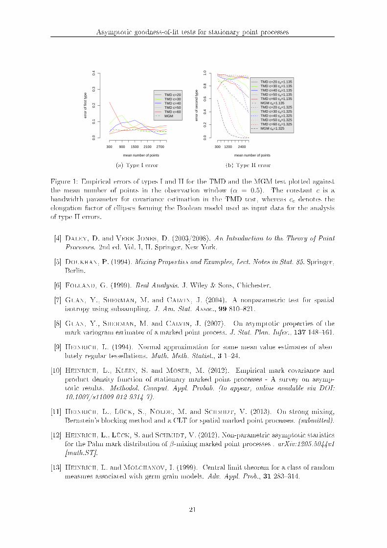
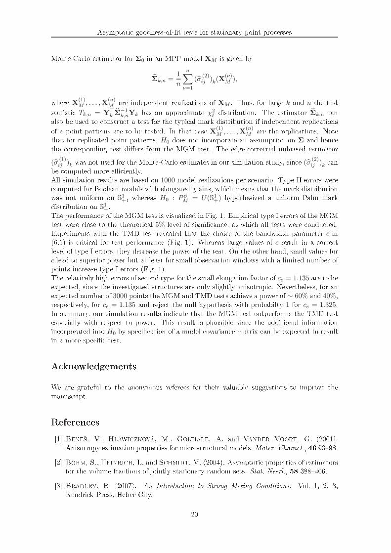
Asymptoti goodness-of-t tests for stationary point pro esses

mean number of points

erro

r of

firs

t typ

e

300 900 1500 2100 2700

0.0

0.1

0.2

0.3

0.4

TMD c=20TMD c=30TMD c=40TMD c=50TMD c=60MGM

(a) Type I error mean number of points

erro

r of

sec

ond

type

300 1200 2400

0.0

0.2

0.4

0.6

0.8

1.0

TMD c=20 ce=1.135TMD c=30 ce=1.135TMD c=40 ce=1.135TMD c=50 ce=1.135TMD c=60 ce=1.135MGM ce=1.135TMD c=20 ce=1.325TMD c=30 ce=1.325TMD c=40 ce=1.325TMD c=50 ce=1.325TMD c=60 ce=1.325MGM ce=1.325(b) Type II errorFigure 1: Empiri al errors of types I and II for the TMD and the MGM test plotted againstthe mean number of points in the observation window (α = 0.5). The onstant c is abandwidth parameter for ovarian e estimation in the TMD test, whereas ce denotes theelongation fa tor of ellipses forming the Boolean model used as input data for the analysisof type II errors.[4 Daley, D. and Vere-Jones, D. (2003/2008). An Introdu tion to the Theory of PointPro esses. 2nd ed. Vol. I, II. Springer, New York.[5 Doukhan, P. (1994). Mixing Properties and Examples, Le t. Notes in Stat. 85. Springer,Berlin.[6 Folland, G. (1999). Real Analysis. J. Wiley & Sons, Chi hester.[7 Guan, Y., Sherman, M. and Calvin, J. (2004). A nonparametri test for spatialisotropy using subsampling. J. Am. Stat. Asso ., 99 810821.[8 Guan, Y., Sherman, M. and Calvin, J. (2007). On asymptoti properties of themark variogram estimator of a marked point pro ess. J. Stat. Plan. Infer., 137 148161.[9 Heinri h, L. (1994). Normal approximation for some mean-value estimates of abso-lutely regular tessellations. Math. Meth. Statist., 3 124.[10 Heinri h, L., Klein, S. and Moser, M. (2012). Empiri al mark ovarian e andprodu t density fun tion of stationary marked point pro esses - A survey on asymp-toti results. Methodol. Comput. Appl. Probab. (to appear, online available via DOI:10.1007/s11009-012-9314-7).[11 Heinri h, L., Lü k, S., Nolde, M. and S hmidt, V. (2013). On strong mixing,Bernstein's blo king method and a CLT for spatial marked point pro esses. (submitted).[12 Heinri h, L., Lü k, S. and S hmidt, V. (2012). Non-parametri asymptoti statisti sfor the Palm mark distribution of β-mixing marked point pro esses . arXiv:1205.5044v1[math.ST.[13 Heinri h, L. andMol hanov, I. (1999). Central limit theorem for a lass of randommeasures asso iated with germ-grain models. Adv. Appl. Prob., 31 283314.21

Asymptoti goodness-of-t tests for stationary point pro esses[14 Heinri h, L. and Pawlas, Z. (2008). Weak and strong onvergen e of empiri aldistribution fun tions from germ-grain pro esses. Statisti s, 42 4965.[15 Heinri h, L. and Proke²ová, M. (2010). On estimating the asymptoti varian e ofstationary point pro esses. Methodol. Comput. Appl. Probab., 12 451471.[16 Kallenberg, O. (1986). Random Measures. A ademi Press, London.[17 Lü k, S., Kups h, A., Lange, A., Hents hel, M. and S hmidt, V. (2012). Sta-tisti al analysis of tomographi re onstru tion algorithms by morphologi al image har-a teristi s. Mater. Res. So . Symp. Pro ., 1421 DOI: 10.1557/opl.2012.209.[18 Midgley, P. and Weyland, M. (2003). 3D ele tron mi ros opy in the physi al s i-en es: the development of Z- ontrast and EFTEM tomography. Ultrami ros opy, 96413431.[19 Pawlas, Z. (2009). Empiri al distributions in marked point pro esses. Sto h. Pro .Appl., 119 41944209.[20 S hneider, R. (1993). Convex Bodies: the Brunn-Minkowski Theory. CambridgeUniversity Press, Cambridge.[21 Yoshihara, K.-I. (1976). Limiting behaviour of U -statisti s for stationary, absolutelyregular pro esses. Z. Wahrs h. verw. Geb., 35 237252.

22