Asymptotic theory of stellar oscillations - AUusers-phys.au.dk/jcd/oscilnotes/chap-7.pdf ·...
46
Chapter 7 Asymptotic theory of stellar oscillations In Chapter 5 I discussed in a qualitative way how different modes of oscillation are trapped in different regions of the Sun. However, the simplified analysis presented there can, with a little additional effort, be made more precise and does in fact provide quite accurate quantitative information about the oscillations. The second-order differential equation (5.17) derived in the previous chapter cannot be used to discuss the eigenfunctions. Thus in Section 7.1 I derive a more accurate second- order differential equation for ξ r . In Section 7.2 the asymptotic solution of such equations by means of the JWKB method is briefly discussed, with little emphasis on mathematical rigour; the results are used to obtain asymptotic expressions for the eigenfrequencies and eigenfunctions. They are used in Sections 7.3 and 7.4 to discuss p and g modes. This approximation, however, is invalid near the surface, and furthermore suffers from critical points in the stellar interior where it formally breaks down. In Section 7.5 I discuss an asymptotic formulation derived by D. O. Gough (cf. Deubner & Gough 1984) that does not suffer from these problems; in particular, it incorporates the atmospheric behaviour of the oscillations analyzed in Section 5.4. On the other hand, it uses a dependent variable with a less obvious physical meaning. This method gives a unified asymptotic treatment of the oscillations throughout the Sun, although still under certain simplifying assumptions. A similar, but even more complete, treatment was developed by Gough (1993), although this appears so far not to have been substantially applied to numerical calculations. One of the most important results of the asymptotic analysis is the so-called Duvall relation, which was first discovered by Duvall (1982) from analysis of observed frequencies of solar oscillation. A rough justification for the relation is given in Section 7.3, and a more rigorous derivation is presented in Section 7.5. It is shown that frequencies of p modes approximately satisfy Z R rt 1 - L 2 c 2 ω 2 r 2 ! 1/2 dr c = [n + α(ω)]π ω . (7.1) This is evidently a very special dependence of the frequencies on n and l. As discussed in Section 7.7, this relation gives considerable insight into the dependence of the frequencies on the sound speed, and it provides the basis for approximate, but quite accurate, methods for inferring the solar internal sound speed on the basis of observed frequencies. 127
Transcript of Asymptotic theory of stellar oscillations - AUusers-phys.au.dk/jcd/oscilnotes/chap-7.pdf ·...

Chapter 7
Asymptotic theory of stellaroscillations
In Chapter 5 I discussed in a qualitative way how different modes of oscillation are trappedin different regions of the Sun. However, the simplified analysis presented there can, witha little additional effort, be made more precise and does in fact provide quite accuratequantitative information about the oscillations.
The second-order differential equation (5.17) derived in the previous chapter cannot beused to discuss the eigenfunctions. Thus in Section 7.1 I derive a more accurate second-order differential equation for ξr. In Section 7.2 the asymptotic solution of such equationsby means of the JWKB method is briefly discussed, with little emphasis on mathematicalrigour; the results are used to obtain asymptotic expressions for the eigenfrequencies andeigenfunctions. They are used in Sections 7.3 and 7.4 to discuss p and g modes. Thisapproximation, however, is invalid near the surface, and furthermore suffers from criticalpoints in the stellar interior where it formally breaks down. In Section 7.5 I discuss anasymptotic formulation derived by D. O. Gough (cf. Deubner & Gough 1984) that doesnot suffer from these problems; in particular, it incorporates the atmospheric behaviour ofthe oscillations analyzed in Section 5.4. On the other hand, it uses a dependent variablewith a less obvious physical meaning. This method gives a unified asymptotic treatment ofthe oscillations throughout the Sun, although still under certain simplifying assumptions.A similar, but even more complete, treatment was developed by Gough (1993), althoughthis appears so far not to have been substantially applied to numerical calculations.
One of the most important results of the asymptotic analysis is the so-called Duvallrelation, which was first discovered by Duvall (1982) from analysis of observed frequenciesof solar oscillation. A rough justification for the relation is given in Section 7.3, and a morerigorous derivation is presented in Section 7.5. It is shown that frequencies of p modesapproximately satisfy
∫ R
rt
(1− L2c2
ω2r2
)1/2dr
c=
[n+ α(ω)]π
ω. (7.1)
This is evidently a very special dependence of the frequencies on n and l. As discussed inSection 7.7, this relation gives considerable insight into the dependence of the frequencieson the sound speed, and it provides the basis for approximate, but quite accurate, methodsfor inferring the solar internal sound speed on the basis of observed frequencies.
127

128 CHAPTER 7. ASYMPTOTIC THEORY OF STELLAR OSCILLATIONS
7.1 A second-order differential equation for ξr
To obtain this equation I go back to the two equations (5.12) and (5.13) in the Cowlingapproximation. By differentiating equation (5.12) and eliminating dp′/dr using equation(5.13) we obtain
d2ξrdr2
= −(
2
r− 1
Γ1H−1p
)dξrdr−[− 2
r2− d
dr
(1
Γ1H−1p
)]ξr
+1
ρc2
(S2l
ω2− 1
)ρ(ω2 −N2)ξr −
1
Γ1H−1p p′
+
[d
drln
∣∣∣∣∣1
ρc2
(S2l
ω2− 1
)∣∣∣∣∣
]p′. (7.2)
Here p′ may be expressed in terms of ξr and its derivative by means of equation (5.12). Theresult is
d2ξrdr2
= −(
2
r− 1
Γ1H−1p
)dξrdr
+
[− 1
Γ1H−1p +
d
drln
∣∣∣∣∣1
ρc2
(S2l
ω2− 1
)∣∣∣∣∣
]dξrdr
+[−K(r) + h(r)]ξr , (7.3)
where K is still given by equation (5.21). All other terms in ξr are lumped together in h;these contain derivatives of equilibrium quantities, and so may be assumed to be negligiblecompared with K (except, as usual, near the surface). Equation (7.3) may also be writtenas
d2ξrdr2− d ln f
dr
dξrdr
+ [K(r)− h(r)]ξr = 0 , (7.4)
where
f(r) =1
ρr2c2
∣∣∣∣∣S2l
ω2− 1
∣∣∣∣∣ . (7.5)
It should be noticed that the principal difference between equation (7.4) and equation(5.20) derived previously is the presence of a term in dξr/dr. This occurs because I have nownot neglected the term in ξr on the right-hand side of equation (5.12), and the correspondingterm in p′ in equation (5.13). These terms cannot be neglected if ξr is rapidly varying, asassumed.
It is convenient to work with an equation without a first derivative, on the form ofequation (5.20). I introduce ξr by
ξr(r) = f(r)1/2ξr(r) ; (7.6)
ξr satisfiesd2ξrdr2
+ [K(r)− h(r)]ξr = 0 , (7.7)
where
h(r) = h(r)− 1
2
d2 ln f
dr2+
1
4
(d ln f
dr
)2
. (7.8)

7.2. THE JWKB ANALYSIS 129
Here h, like h, is generally small compared with K. When it is neglected asymptotically,equation (7.7) is identical to equation (5.20), apart from the change of the dependentvariable. In particular, the trapping properties of the modes, as inferred from this analysis,are the same as obtained previously.
It is obvious that the derivation of equation (7.7) fails near points where ω2 = S2l , and
where consequently f has a singular logarithmic derivative. These are the turning pointsof p modes. This problem can be avoided by deriving instead a second-order differentialequation for p′ (see Unno et al. 1989, Chapter 16); but, hardly surprisingly, this equationhas problems at the turning points for the g modes. It is possible to develop a coherentasymptotic theory by suitably combined use of these two equations; a more convenientapproach, however, is to use a second-order equation that is valid throughout the model.I return to this in Section 7.5, but base the initial asymptotic analysis on the somewhatsimpler equation (7.7).
7.2 The JWKB analysis
To analyze equation (7.7) asymptotically I use the JWKB method (for Jeffreys, Wentzel,Kramers and Brillouin; in fact the method seems to have been first used by Liouville). It iswidely used in quantum mechanics (see e.g. Schiff 1949, Section 34), and is also describedin Unno et al. (1989), Chapter 16. It is possible to provide a firm mathematical foundationfor the method; knowing that this is so, it is enough here to sketch how it works, withoutworrying too much about its convergence properties.
The assumption is that the solution varies rapidly compared with equilibrium quantities,i.e., compared with K(r). Thus I write it as
ξr(r) = a(r) exp[iΨ(r)] , (7.9)
where Ψ is rapidly varying, so that the local radial wave number
kr =dΨ
dr(7.10)
is large; a(r) is a slowly varying amplitude function. Formally, it is always possible to writethe solution in this form. If equation (7.9) is substituted into equation (7.7), neglecting h,one obtains
(d2a
dr2+ 2ikr
da
dr+ ia
dkrdr− k2
ra
)exp(iΨ) = −K(r)a(r) exp(iΨ) . (7.11)
On the left-hand side the dominant term is the one containing k2r ; to ensure that this term
cancels with the right-hand side, kr must be chosen as
kr(r) = K(r)1/2 . (7.12)
The next-order terms are those in kr which must cancel. Thus
1
a
da
dr= −1
2
1
kr
dkrdr
, (7.13)
or, apart from a constant factor,
a(r) = |kr|−1/2 = |K(r)|−1/4 . (7.14)

130 CHAPTER 7. ASYMPTOTIC THEORY OF STELLAR OSCILLATIONS
This leaves in equation (7.11) only a term in the second derivative of a. The asymptoticapproximation consists of neglecting this term, which by the assumption is small comparedwith k2
ra. Then the approximate solution is completely specified by equations (7.12) and(7.14). Since the solution may be chosen to be real, it can be written as
ξr(r) = A |K(r)|−1/4 cos
(∫ r
r0K(r′)1/2dr′ + φ
), for K(r) > 0 , (7.15)
or
ξr(r) = |K(r)|−1/4[A+ exp
(∫ r
r0|K(r′)|1/2dr′
)+A− exp
(−∫ r
r0|K(r′)|1/2dr′
)]
for K(r) < 0 , (7.16)
for some suitable r0. Here A and φ, or A+ and A−, are real constants which must bedetermined from the boundary conditions.
Notice that this solution has the property of being locally exponential where K < 0.Thus it is in accordance with the discussion in Section 5.2. On the other hand, it breaksdown at the zeros of K; formally this may be seen from the fact that there a, as obtainedin equation (7.12), is singular, and its second derivative cannot be neglected in equation(7.11). Thus we need to make a special analysis of the points where K = 0. In particular,this is required to connect the solution in the exponential and oscillatory regions, and henceapply the boundary conditions.
I consider a turning point r1 such that K(r) < 0 for r < r1 and K(r) > 0 for r > r1. Ifr1 is a simple zero for K, close to r1 we have approximately that
K(r) ' K1(r − r1) , (7.17)
where K1 > 0 is a constant. I introduce the new independent variable x by
x = K1/31 (r − r1) ; (7.18)
then the equation for ξr can be approximated by
d2ξrdx2
= −xξr , (7.19)
with the solutionξr(r) = C1Ai (−x) + C2Bi (−x) , (7.20)
where C1 and C2 are constants, and Ai and Bi are the Airy functions (e.g. Abramowitz &Stegun 1964).
To be definite, I consider a solution that is trapped in the oscillatory region outside r1,and hence we need to choose the constants C1 and C2 such as to select the solution thatdecreases exponentially as r decreases beneath r1. When x < 0, and |x| is large, Ai (−x)and Bi (−x) have the following asymptotic behaviour:
Ai (−x) ' 1
2√π|x|−1/4 exp
(−2
3|x|3/2
),
Bi (−x) ' 1√π|x|−1/4 exp
(2
3|x|3/2
). (7.21)

7.2. THE JWKB ANALYSIS 131
Thus we must require that C2 = 0, and the solution satisfying the boundary condition forr < r1 is therefore
ξr(r) = C1Ai (−x) . (7.22)
We can use this solution to determine the phase φ in equation (7.15). For large positivex the asymptotic expansion of Ai (−x) is
Ai (−x) ' 1√π|x|−1/4 cos
(2
3x3/2 − π
4
). (7.23)
This must agree with what is obtained from equation (7.15), assuming that there is a regionwhere both this equation and the approximation in equation (7.23) are valid. From theexpansion of K in equation (7.17) we obtain
Ψ =
∫ r
r1K(r′)1/2dr′ + φ =
2
3x3/2 + φ , (7.24)
so that equation (7.15) gives
ξr ' AK−1/61 x−1/4 cos
(2
3x3/2 + φ
). (7.25)
This agrees with equation (7.23) if
φ = −π4. (7.26)
Sufficiently far from the turning point r1 the JWKB solution satisfying the boundary con-ditions at r = r1 is thus
ξr(r) = A1|K(r)|−1/4 cos
(∫ r
r1K(r′)1/2dr′ − π
4
). (7.27)
Similarly, if there is an outer turning point at r = r2, so that K(r) > 0 for r < r2 andK(r) < 0 for r > r2, one finds that the asymptotic solution that is exponentially decayingfor r > r2 is
ξr(r) = A2|K(r)|−1/4 cos
(∫ r2
rK(r′)1/2dr′ − π
4
). (7.28)
Exercise 7.1:
Verify this.
To obtain the full solution we must match the two separate solutions smoothly at asuitable point between r1 and r2, r = rf , say. I define
Ψ1 ≡ Ψ1(rf) =
∫ rf
r1K(r)1/2dr − π
4,
Ψ2 ≡ Ψ2(rf) =
∫ r2
rf
K(r)1/2dr − π
4. (7.29)

132 CHAPTER 7. ASYMPTOTIC THEORY OF STELLAR OSCILLATIONS
Then the conditions that both ξr and its first derivative be continuous at r = rf give
A1K(rf)−1/4 cos Ψ1 = A2K(rf)
−1/4 cos Ψ2 ,
−A1K(rf)−1/4 sin Ψ1 = A2K(rf)
−1/4 sin Ψ2 . (7.30)
Notice that in the derivative I have neglected terms coming from the differentiation of K;these are small compared with the term included. These linear equations for A1, A2 onlyhave a non-trivial solution if their determinant vanishes. This leads to
sin Ψ1 cos Ψ2 + cos Ψ1 sin Ψ2 = sin(Ψ1 + Ψ2) = 0 , (7.31)
orΨ1 + Ψ2 = (n− 1)π , (7.32)
where n is an integer. Thus∫ r2
r1K(r)1/2dr = (n− 1
2)π, n = 1, 2, . . . . (7.33)
Here K depends on the frequency ω; thus equation (7.33) implicitly determines the fre-quencies of the modes trapped between r1 and r2. In addition, we find that A1 = A2.
We can also find the asymptotic behaviour of the eigenfunctions. From the definitionof ξr, equations (7.5) and (7.6), it follows from equation (7.27) that for r1 < r < r2
ξr(r) = Aρ−1/2r−1c−1
∣∣∣∣∣S2l
ω2− 1
∣∣∣∣∣
1/2
|K(r)|−1/4 cos
(∫ r
r1K(r′)1/2dr′ − π
4
)
= Aρ−1/2r−1c−1/2
∣∣∣∣∣S2l /ω
2 − 1
N2/ω2 − 1
∣∣∣∣∣
1/4
cos
(∫ r
r1K(r′)1/2dr′ − π
4
), (7.34)
where A = A ω−1/2. This expression is clearly valid only at some distance from the turningpoints, where the asymptotic approximation (7.23) can be used. Thus the apparentlysingular behaviour in | · · · | causes no problems.
Notice that in equation (7.34) c−1/2 (which is proportional to T−1/4) and | · · · |1/4 varyrelatively little through the region where the modes are trapped. Thus the variation of ξrthrough the Sun is dominated by ρ−1/2r−1. This is the reason why I plotted the eigenfunc-tion in terms of ρ1/2rξr(r) in Figures 5.8 and 5.10.
We can also find the solution in the exponential regions, by using the asymptotic expan-sion for Ai in equation (7.21). The results are, for the solution corresponding to equation(7.34) in the trapping region
ξr(r) '1
2Aρ−1/2r−1c−1/2
∣∣∣∣∣S2l /ω
2 − 1
N2/ω2 − 1
∣∣∣∣∣
1/4
exp
(−∫ r1
r
∣∣K(r′)∣∣1/2 dr′
)
for r < r1 , (7.35)
and
ξr(r) '1
2Aρ−1/2r−1c−1/2
∣∣∣∣∣S2l /ω
2 − 1
N2/ω2 − 1
∣∣∣∣∣
1/4
exp
(−∫ r
r2
∣∣K(r′)∣∣1/2 dr′
)
for r > r2 . (7.36)

7.3. ASYMPTOTIC THEORY FOR P MODES 133
7.3 Asymptotic theory for p modes
For high frequencies we may, as in Section 5.2, approximate K by
K(r) ' 1
c2(ω2 − S2
l ) . (7.37)
As discussed previously the theory, as formulated so far, does not provide reflection at thesurface. Mathematically, this is expressed by the lack of a turning point near the surface.Also, the formulation fails near the point where ω = Sl where the neglected term h(r)in (7.8) is singular. Thus equation (7.33) for the eigenfrequencies cannot immediately beused. It is shown in Section 7.5 below that a proper treatment of the surface and the lowerturning point leads to an asymptotic behaviour similar to that discussed above; however,the effective phase shift in the equation corresponding to (7.33) is different. Thus thefrequencies for the p modes approximately satisfy
∫ R
rt(ω2 − S2
l )1/2 dr
c= (n+ α)π , (7.38)
where α is a new phase constant, which contains the contribution 1/4 from the innerturning point, and an, as yet unidentified, contribution from the outer turning point. It isconvenient to write this equation as
∫ R
rt
(1− L2
ω2
c2
r2
)1/2dr
c=
(n+ α)π
ω, (7.39)
where L2 = l(l+1). Notice that the left-hand side of this equation is a function of w = ω/L[it follows from equation (5.28) that rt is determined by ω/L]; thus equation (7.39) can bewritten as
π(n+ α)
ω= F
(ω
L
), (7.40)
where
F (w) =
∫ R
rt
(1− c2
r2w2
)1/2dr
c. (7.41)
The observed and computed frequencies in fact satisfy relations like equation (7.40) quiteclosely; this was first noticed by Duvall (1982) for the observed frequencies. An example isillustrated in Figure 7.1.
When the function F (w) is known from observations, equation (7.41) can be invertedto determine c(r). I return to this in Section 7.7.
It is instructive to consider a special case of this equation, which is furthermore a reason-able approximation to the Sun. The solar convection zone is approximately adiabaticallystratified, so that
d ln p
dr= Γ1
d ln ρ
dr; (7.42)
here I assume Γ1 to be constant (this is evidently not true in the ionization zones of Hand He, but they only occupy the outer few per cent of the Sun). We may also assumethat g is constant. Finally I take as boundary conditions on the equilibrium structure thatp = ρ = 0 at r = R. With these assumptions the sound speed is given by
c2 =g
µp(R− r) , (7.43)

134 CHAPTER 7. ASYMPTOTIC THEORY OF STELLAR OSCILLATIONS
Figure 7.1: Observed frequencies of solar oscillation, plotted according to equa-tion (7.40). The constant value of α, 1.45, was determined such as to minimizethe spread in the relation (7.40). (Adapted from Christensen-Dalsgaard et al.1985.)
where µp = 1/(Γ1− 1) is an effective polytropic index of the region considered. I also treatthe layer as plane parallel, so that r can be replaced by R in the integral in equation (7.41).Then the integral may easily be evaluated, to yield
F (w) =π
2wµpR
g. (7.44)
Exercise 7.2:
Derive equations (7.43) and (7.44).
Thus the dispersion relation (7.40) gives
ω2 =2
µp
g
R(n+ α)L . (7.45)

7.3. ASYMPTOTIC THEORY FOR P MODES 135
In particular, ω is proportional to L1/2. This property is approximately satisfied by thecomputed (and observed) frequencies at high degree (cf. Figure 5.6). Indeed, equation(7.45) might be expected to be approximately valid for modes whose degree is so high thatthey are entirely trapped within the convection zone.
For modes of low degree, rt is very close to the centre (see Figure 5.5). In equation(7.39), therefore, the second term in the bracket on the left-hand side is much smaller thanunity over most of the range of integration. To exploit this, I consider the difference
I =
∫ R
0
dr
c−∫ R
rt
(1− c2
w2r2
)1/2dr
c
=
∫ rt
0
dr
c+
∫ R
rt
1−
(1− c2
w2r2
)1/2 dr
c
≡ I1 + I2 , (7.46)
where w = ω/L. Notice that c is almost constant near the centre (it may be shown thatthe first derivative of c is zero at r = 0). Thus I take c to be constant in the first integral,and obtain
I1 =rt
c(0)' L
ω=
1
w, (7.47)
by using equation (5.28). In the second integral the integrand is only substantially differentfrom zero for r close to rt, which was assumed to be small. Thus here I also approximate cby its value at r = 0. Furthermore, the upper limit of integration may be replaced by ∞.Then we obtain
I2 =1
w
∫ 1
0
[1−
(1− u2
)1/2]
du
u2=
1
w
(π
2− 1
). (7.48)
Thus, finally,
I =1
w
π
2, (7.49)
and equation (7.39) may be approximated by
∫ R
0
dr
c− L
ω
π
2=
(n+ α)π
ω, (7.50)
or
ω =(n+ L/2 + α)π
∫ R
0
dr
c
. (7.51)
The derivation of equation (7.51) clearly lacks rigour. However, it may be shown froma more careful asymptotic analysis of the central region (e.g. Vandakurov 1967; Tassoul1980) that the result is correct to leading order, except that L should be replaced by l+1/2.Equation (7.51) may also be written as
νnl =ωnl2π' (n+
l
2+
1
4+ α)∆ν , (7.52)
where
∆ν =
[2
∫ R
0
dr
c
]−1
(7.53)

136 CHAPTER 7. ASYMPTOTIC THEORY OF STELLAR OSCILLATIONS
is the inverse of twice the sound travel time between the centre and the surface. Thisequation predicts a uniform spacing ∆ν in n of the frequencies of low-degree modes. Also,modes with the same value of n+ l/2 should be almost degenerate,
νnl ' νn−1 l+2 . (7.54)
This frequency pattern has been observed for the solar five-minute modes of low degree(cf. Chapter 2), and may be used in the search for stellar oscillations of solar type. Infact, as shown in Figure 5.14 it is visible even down to very low radial order for computedfrequencies of models near the zero-age main sequence.
The deviations from the simple relation (7.52) have considerable diagnostic potential.The expansion of equation (7.39), leading to equation (7.51), can be extended to take intoaccount the variation of c in the core (Gough 1986a); alternatively it is possible to take theJWKB analysis of the oscillation equations to higher order (Tassoul 1980). The result maybe written as
νnl ' (n+l
2+
1
4+ α)∆ν − (AL2 − δ)∆ν2
νnl, (7.55)
where
A =1
4π2∆ν
[c(R)
R−∫ R
0
dc
dr
dr
r
]. (7.56)
Hence
δνnl ≡ νnl − νn−1 l+2 ' −(4l + 6)∆ν
4π2νnl
∫ R
0
dc
dr
dr
r, (7.57)
where I neglected the term in the surface sound speed c(R). It is often convenient to rep-resent observed or computed frequencies in terms of a limited set of parameters associatedwith the asymptotic description of the modes. This may be accomplished by fitting theasymptotic expression to the frequencies. By carrying out a polynomial fit in the quan-tity x − x0, where x = n + l/2 and x0 is a suitable reference value (Scherrer et al. 1983,Christensen-Dalsgaard 1988b) one obtains the average over n of δνnl as
〈δνnl〉n ' (4l + 6)D0 , (7.58)
where
D0 ' −1
4π2x0
∫ R
0
dc
dr
dr
r. (7.59)
Thus δνnl is predominantly determined by conditions in the stellar core. Physically, this maybe understood from the fact that only near the centre is kh comparable with kr. Elsewherethe wave vector is almost vertical, and the dynamics of the oscillations is largely independentof their horizontal structure, i.e., of l; therefore at given frequency the contributions of theselayers to the frequency are nearly the same, and hence almost cancel in the difference inequation (7.57).
It should be noted that the accuracy of expressions (7.58) and (7.59) is questionable;they appear to agree fortuitously with frequencies computed for models of the presentSun, whereas they are less successful for models of different ages or masses (Christensen-Dalsgaard 1991a). However, the form of the dependence of 〈δνnl〉n on l shown in equation(7.58), as well as the argument that this quantity is most sensitive to conditions in stellarcores, probably have a broader range of validity. As a star evolves, the hydrogen abundance

7.3. ASYMPTOTIC THEORY FOR P MODES 137
in the core decreases and hence the mean molecular weight increases. For an approximatelyideal gas, the sound speed may be obtained from
c2 ' kBT
µmu; (7.60)
since the central temperature varies little during hydrogen burning, due to the strongtemperature sensitivity of the nuclear reaction rates, the main effect on the sound speed inthe core comes from the change in the mean molecular weight µ. Consequently c decreasesas the star evolves, the decrease being most rapid at the centre where hydrogen burning isfastest. As a result, c develops a local minimum at the centre, and dc/dr is positive in thecore. This region gives a negative contribution to D0 (cf. eq. 7.57), of increasing magnitudewith increasing age, and hence D0 decreases with increasing age (see also Christensen-Dalsgaard 1991a). Hence D0, which can in principle be observed, is a measure of theevolutionary state of the star. On the other hand, the overall frequency separation ∆ν,defined in equation (7.53), approximately scales as the inverse of the dynamical time scalewhich, for main-sequence stars, is largely determined by the mass.
These considerations motivate presenting the average frequency separations in a(∆ν0, D0) diagram, as illustrated in Figure 7.2; this is analogous to the ordinaryHertzsprung-Russell diagram. As shown in panel (b) (note the different scales) most ofthe variation in ∆ν0 is in fact related to tdyn, such that ∆ν0 scales as M1/2/R3/2. It isevident from Figure 7.2 that on the assumption that the other parameters of the star (suchas composition) are known, a measurement of ∆ν and D0 may allow determination of themass and evolutionary state of the star (Christensen-Dalsgaard 1984b; Ulrich 1986, 1988;Christensen-Dalsgaard 1988b). On the other hand, Gough (1987) analyzed the sensitiv-ity of this result to the other stellar parameters, and found that the uncertainty in theknowledge of the heavy element abundance, in particular, had a severe effect on the de-termination of the mass and age. As an example of such sensitivity, Figure 7.2(c) showsthe consequences of an increase of the hydrogen abundance by 0.03. A careful analysisof the information content in measured frequency separations, when combined with moretraditional measurements of stellar properties, was given by Brown et al. (1994).
The eigenfunctions of p modes can be found from equation (7.34). It is convenient touse equation (7.38) to get
∫ r
rtK(r′)1/2dr′ = −
∫ R
rK(r′)1/2dr′ + (n+ α)π , (7.61)
so that we obtain
ξr(r) ' (7.62)
Aρ−1/2c−1/2r−1
∣∣∣∣∣1−S2l
ω2
∣∣∣∣∣
1/4
cos
ω∫ R
r
(1− S2
l
ω2
)1/2dr′
c− (−1/4 + α)π
,
where I have again neglected N 2/ω2. However, the derivation neglects the fact that thepresent simple asymptotic description breaks down near the lower turning point. As shownin Section 7.5, a more appropriate treatment gives essentially the same result, except thatthe term −1/4 in equation (7.62) must be replaced by 1/4. Also, to simplify this expressionfurther I note that S2
l decreases quite rapidly with increasing r. Near r = rt, ω2 and S2
l are

138 CHAPTER 7. ASYMPTOTIC THEORY OF STELLAR OSCILLATIONS
Figure 7.2: Evolution tracks ( ) and curves of constant central hy-drogen abundance ( ) in (∆ν0, D0) diagrams. Here ∆ν0 is the aver-age separation between modes of the same degree and adjacent radial order,and D0 is related to the small separation between νnl and νn−1 l+2 (cf. eq.7.58). The stellar masses, in solar units, and the values of the central hydro-gen abundance, are indicated. In panel (b), the frequency separations havebeen scaled by (ρ)−1/2 (ρ ∝ M/R3 being the mean density), to take out thevariation with t−1
dyn. Panel (c) shows the effect of increasing the hydrogenabundance by 0.03 (heavy lines), relative to the case presented in panel (a)(shown here with thin lines). (From Christensen-Dalsgaard 1993b.)

7.3. ASYMPTOTIC THEORY FOR P MODES 139
comparable, but at some distance from the turning point we can assume that S2l /ω
2 1.Here, therefore
ξr(r) ' Aρ−1/2c−1/2r−1 cos
[ω
∫ R
r
dr′
c− (1/4 + α)π
]. (7.63)
To this approximation the eigenfunction is independent of l. Oscillations with the samefrequency but different l therefore have approximately the same eigenfunctions near thesurface, if they are normalized to the same surface value. This was also seen in Figure5.8. This property is important for the interpretation of the observed frequencies. It maybe understood physically in the following way: near the surface the vertical wavelength ismuch shorter than the horizontal wavelength (i.e., kr kh); the tangential component ofthe displacement therefore has essentially no influence on the dynamics of the oscillation,which is consequently independent of l.
Figure 7.3: Scaled eigenfunction for radial p mode of order n = 23 and fre-quency ν = 3310µHz in a normal solar model (the same mode as was shownin Figure 5.8a). According to the asymptotic equation (7.63) the quantityplotted should oscillate between fixed limits in the region where the mode istrapped.
From equation (7.63) one should expect that c1/2ρ1/2r ξr(r) behaves like a cosine func-tion with a non-uniform argument. This is confirmed to high accuracy by Figure 7.3. Thusequation (7.63) in fact gives a reasonable description of the eigenfunctions of high-order pmodes in the region where they are trapped.

140 CHAPTER 7. ASYMPTOTIC THEORY OF STELLAR OSCILLATIONS
7.4 Asymptotic theory for g modes
For these in general ω2 S2l , and I approximate K by
K(r) ' l(l + 1)
r2
(N2
ω2− 1
). (7.64)
Typically a mode is trapped between two zeros r1 and r2 of K, and equation (7.33) isimmediately valid. Thus the frequencies are determined by
∫ r2
r1L
(N2
ω2− 1
)1/2dr
r= (n− 1/2)π , (7.65)
or∫ r2
r1
(N2
ω2− 1
)1/2dr
r=
(n− 1/2)π
L. (7.66)
Here the left-hand side is solely a function of ω, so that equation (7.66) can be written, inanalogy with equation (7.40), as
n− 1/2
L= G(ω) , (7.67)
where
G(ω) =1
π
∫ r2
r1
(N2
ω2− 1
)1/2dr
r. (7.68)
I have here implicitly assumed that N has a single maximum, so that there is a single,well-defined trapping region at each frequency. In many stellar models, including somemodels of the Sun, there may be several maxima in N , and this may give rise to, atleast mathematically, interesting phenomena. Roughly speaking, to each maximum therecorresponds asymptotically a separate spectrum of g modes; where modes correspondingto different regions happen to have nearly the same frequencies, the modes may interact in“avoided crossings” (e.g. Christensen-Dalsgaard, Dziembowski & Gough 1980).
In the model illustrated in Figure 5.2 N has a weak secondary maximum near r/R =0.35, and at a frequency of about 410µHz; this is in fact faintly reflected in the behaviourof the frequencies shown in Figure 5.6, where there is an accumulation of modes at thisfrequency, for l > 15. I neglect this local maximum and assume that N has a singlemaximum, Nmax, in the interior of the Sun; from equation (7.68) it then follows that
G(ω)→ 0 for ω → Nmax . (7.69)
Consequentlyω → Nmax for L→∞ . (7.70)
This behaviour is clearly visible in Figures 5.6 and 5.7.For high-order, low-degree g modes ω is much smaller than N over most of the interval
[r1, r2]. This suggests that a similar approximation to the one leading to equation (7.51)should be possible. In fact, the integral may be expanded near the centre, in much the sameway as the integral in equation (7.39), by using the fact that N ∼ r near r = 0. However,the expansion near the upper turning point can apparently not be done in a similarly

7.4. ASYMPTOTIC THEORY FOR G MODES 141
simple fashion, and in any case the result does not quite have the correct dependence onl. A proper asymptotic analysis (Tassoul 1980) shows that the frequencies of low-degree,high-order g modes are given by
ω =
L
∫ r2
r1N
dr
r
π(n+ l/2 + αg), (7.71)
where αg is a phase constant. Thus in this case the periods are asymptotically equallyspaced in the order of the mode. The spacing decreases with increasing l, as is also obviousfrom Figure 5.6.
The analysis was carried to the next asymptotic order by Tassoul (1980). Ellis (1988),Provost & Berthomieu (1986) and Gabriel (1986) compared the resulting expressions withnumerically computed frequencies for polytropic or solar models.
In the trapping region the eigenfunction is given by equation (7.34). We may assumethat ω2 S2
l , and so obtain
ξr(r) ' Aρ−1/2r−1c−1/2(Slω
)1/2∣∣∣∣∣N2
ω2− 1
∣∣∣∣∣
−1/4
cos
L
∫ r
r1
(N2
ω2− 1
)1/2dr′
r′− π
4
= A
(L
ω
)1/2
ρ−1/2r−3/2
∣∣∣∣∣N2
ω2− 1
∣∣∣∣∣
−1/4
cos
L
∫ r
r1
(N2
ω2− 1
)1/2dr′
r′− π
4
. (7.72)
Except close to the turning points r1, r2 we may assume that N 2/ω2 1 (note, from Figure5.2, that N increases very rapidly from 0 at the centre and at the base of the convectionzone). Here, therefore,
ξr(r) ' AL1/2ρ−1/2r−3/2N−1/2 cos
L
∫ r
r1
(N2
ω2− 1
)1/2dr′
r′− π
4
. (7.73)
Hence we expect that ρ1/2r3/2N1/2ξr behaves like a distorted cosine function. This isconfirmed by Figure 7.4. Thus equation (7.73), as the corresponding equation for the pmodes, gives a fairly accurate description of the eigenfunction in the trapping region.
Outside the trapping region the eigenfunction locally decays exponentially; this is alsodescribed by saying that the mode is evanescent. In particular, g modes are always evanes-cent in convection zones. From Figure 5.2 it follows that in the solar case this evanescentregion is essentially restricted to the convection zone for ν < 200µHz. At higher frequenciesthe evanescent region extends more deeply, and for frequencies near the maximum in Nthe mode is oscillatory only in a narrow region around x = 0.1. Thus one would expectsuch modes to be very efficiently trapped. To study the trapping I use the asymptoticexpression (7.36). In the convection zone we can assume that N = 0; and for low-frequency(and high-degree) modes I neglect ω2/S2
l compared with 1. Then K ' −L2/r2, and thevariation in ξr through the convection zone may be approximated by
ξr(r) '1
2
(L
ω
)1/2
ρ−1/2r−3/2 exp
(−L
∫ r
r2
dr′
r′
)
=1
2
(L
ω
)1/2
r2Lρ−1/2r−(3/2+L) . (7.74)

142 CHAPTER 7. ASYMPTOTIC THEORY OF STELLAR OSCILLATIONS
Figure 7.4: Scaled eigenfunction for high-order g mode of degree 2, radialorder n = −10 and frequency ν = 104µHz in a normal solar model (the samemode as was shown in Figure 5.10b). According to the asymptotic equation(7.73) the quantity plotted should oscillate between fixed limits in the regionwhere the mode is trapped.
Thus the density decrease with increasing radius causes an increase in the amplitude, butthis is compensated for by the power law decrease represented by r−L (note that this isthe global manifestation of the locally exponential behaviour in the evanescent region). Toget an idea about the relative importance of these two effects I note that the radius rb atthe base of the solar convection zone is about 0.7 R, whereas the ratio between the surfacedensity and the density at the base of the convection zone is about 10−6. Thus we obtain
ξr(rb)/ξr(R) ∼ 10−3(0.7)−(3/2+L) ∼ 10−2.8+0.15L . (7.75)
This approximation, however, assumed the validity of the asymptotic expression (7.36)right up to the surface. This is not true, as the assumptions underlying the analysis breakdown close to the surface where the pressure scale height becomes small. It appears thatthese effects dominate unless l is quite large. An attempt at analyzing this, based on themore complete asymptotic theory to be described in the following section, is provided inSection 7.6.2.
This analysis roughly describes the trapping of low-frequency modes. At higher fre-quencies the deepening of the evanescent region must also be taken into account, and theasymptotic analysis becomes rather complicated. Reference may be made, however, to thenumerical results presented in Figures 5.12 and 5.13. At low frequencies the increase in theinterior amplitude with degree, at fixed frequency, is roughly in accordance with the asymp-totic discussion given above. The steep increase with increasing frequency at ν > 400µHzis related to the faint local maximum in N at that frequency, which was discussed above(cf. Figure 5.2); modes with higher frequency suddenly get trapped much deeper in the

7.5. A GENERAL ASYMPTOTIC EXPRESSION 143
Sun, and their maximum amplitudes consequently rise very rapidly. For comparison onemight note that a mode with a velocity amplitude of 1 m sec−1 and a period of 1 hour hasa relative surface displacement amplitude of about 10−6. Thus modes with an amplituderatio of more than 106 are not likely to be seen. Clearly there is little hope of observing gmodes of degree greater than 20.
A more careful analysis than presented here would probably allow an understanding ofmany of the features shown in Figures 5.12 and 5.13. This would be interesting but has, asfar as I know, not been undertaken so far.
7.5 A general asymptotic expression
An approximate asymptotic description of the oscillations has been derived by Gough (seeDeubner & Gough 1984), on the basis of earlier work by Lamb (1932). This does notassume that the pressure and density scale heights are much larger than the wavelength;but it assumes that the oscillations vary much more rapidly than r and g, so that theproblem is locally one of oscillations of a plane-parallel layer under constant gravity. Also,as usual, the perturbation in the gravitational potential is neglected. Then the governingequations are equations (5.12) and (5.13), but without the term in 2/r in the former. Whenmanipulating the equations, I neglect derivatives of r and g, but keep derivatives of thethermodynamic quantities. I note that Gough (1993) generalized this treatment to includealso sphericity and varying gravity, although at the expense of obtaining considerably morecomplicated expressions.
7.5.1 Derivation of the asymptotic expression
The trick of the analysis is to write the equations in terms of
χ = div δδδr . (7.76)
By using the equation of continuity and the condition of adiabaticity we may also write χas
χ = − 1
Γ1
(p′
p− ρg
pξr
). (7.77)
The oscillation equations can be written as
dξrdr
= χ+1
ρ
k2h
ω2p′ , (7.78)
anddp′
dr= ρ
(ω2 + g
d ln ρ
dr
)ξr + gρχ . (7.79)
In keeping with the plane-parallel approximation I have expressed l by kh, given by equation(4.51), and I assume kh to be constant.
By multiplying equation (7.77) by Γ1p and differentiating we obtain, on using equations(7.78) and (7.79)
dΓ1
drpχ− Γ1gρχ+ Γ1p
dχ
dr= −ρω2ξr +
gk2h
ω2p′ . (7.80)

144 CHAPTER 7. ASYMPTOTIC THEORY OF STELLAR OSCILLATIONS
This equation, together with equation (7.77), can be used to express ξr in terms of χ andits first derivative. The result is
ρ
(g − ω4
gk2h
)ξr = Γ1
[pχ+
ω2
gk2h
(p
dχ
dr− gρχ+ p
d ln Γ1
drχ
)]. (7.81)
Finally, by differentiating equation (7.80) and using equations (7.78), (7.79) and (7.81)to eliminate ξr, p
′ and their derivatives, we obtain the following second-order differentialequation for χ:
d2χ
dr2+
(2
c2
dc2
dr+
1
ρ
dρ
dr
)dχ
dr(7.82)
+
[1
Γ1
d2Γ1
dr2− 2
Γ1
dΓ1
dr
gρ
p+ k2
h
(N2
ω2− 1
)− 1
ρ
dρ
dr
1
Γ1
dΓ1
dr+ρω2
Γ1p
]χ = 0 .
Here I have introduced the adiabatic sound speed c from equation (3.52) and the buoyancyfrequency N from equation (3.73).
The differential equation for χ contains no interior singular points. However, it is clearfrom equation (7.81) that the case where the coefficient of ξr vanishes is in some sensesingular. This occurs when
ω2 = gkh . (7.83)
It is easy to show that then the solution for χ to equation (7.81) grows exponentially towardsthe interior; as this is clearly unacceptable, χ must be zero. Then equation (7.77) gives
p′ = gρξr , (7.84)
and equation (7.78) has the solution
ξr = a exp(khr) , (7.85)
where a is an arbitrary constant. It is easy to show that the resulting p′ satisfies equation(7.79). Thus this is one possible solution to the plane-parallel oscillation equations. Itshould be noticed that equation (7.83) agrees with equation (3.84) for the frequency of asurface gravity wave. Thus the mode we have found must be identified with a surface gravitywave; and we have shown that its frequency is independent of the structure of the modelbelow the surface, if sphericity is neglected. This result was first obtained by Gough. It isobvious from Figure 5.6 that the mode can be followed to degrees well below 10, althoughhere the correction to the frequency given by equation (7.83) becomes significant.
To analyze equation (7.82) it is convenient to eliminate the term in dχ/dr. Thus Iintroduce X by
X = c2ρ1/2χ . (7.86)
After considerable manipulation one then finds that X satisfies the differential equation
d2X
dr2+
[k2
h
(N2
ω2− 1
)+ω2
c2− 1
2
d
dr(H−1)− 1
4H−2
]X = 0 , (7.87)
where I have introduced the density scale height H by
H−1 = −d ln ρ
dr. (7.88)

7.5. A GENERAL ASYMPTOTIC EXPRESSION 145
Finally, I define a characteristic frequency ωc by
ω2c =
c2
4H2
(1− 2
dH
dr
), (7.89)
and use equation (4.60) for the acoustic frequency Sl, to obtain
d2X
dr2+
1
c2
[S2l
(N2
ω2− 1
)+ ω2 − ω2
c
]X = 0 . (7.90)
This is the final second-order differential equation. Considering that the only approxima-tions made in deriving it are the constancy of g and the neglect of the derivatives of r, it isremarkably simple.
Figure 7.5: The acoustical cut-off frequency ωc defined in equation (7.89)(solid line), and the approximation ωa appropriate to an isothermal region [cf.equation (5.45); dashed line] in the outermost parts of a normal model of thepresent Sun.
It might be noticed that equation (7.90) can also be derived from a careful analysis ofthe propagation of waves in stellar interiors. This has been carried out by Gough (1986a).
Notice that if H is constant (as was assumed in Section 5.4), equation (7.89) for ωc
reduces to the frequency ωa defined in equation (5.45). Thus ωc, as introduced here, gen-eralizes the acoustical cut-off frequency defined for the isothermal atmosphere. Figure 7.5shows ωc and ωa in the outer parts of a normal solar model; they are in fact quite similar,except in a thin region very near the top of the convection zone, where the rapid variationin the superadiabatic gradient causes large excursions in ωc.
Near the surface S2l is small, and the coefficient of X in equation (7.90) is dominated
by the last two terms; hence X is exponential when ω2 < ω2c . This provides the trapping

146 CHAPTER 7. ASYMPTOTIC THEORY OF STELLAR OSCILLATIONS
of the modes at the surface. In the interior ω2c (which roughly varies as g2/T ) is generally
small, below about 600µHz in models of the present Sun.We may write equation (7.90) as
d2X
dr2+K(r)X = 0 , (7.91)
where
K(r) =ω2
c2
[1− ω2
c
ω2− S2
l
ω2
(1− N2
ω2
)]
≡ ω2
c2
(1−
ω2l,+
ω2
)(1−
ω2l,−ω2
), (7.92)
defining the characteristic frequencies ωl,+ and ωl,−. They are plotted in Figure 7.6, ina model of the present Sun. Equation (7.92) shows that the trapping of the modes isdetermined by the value of the frequency, relative to behaviour of ωl,+ and ωl,−. In theinterior of the Sun, particularly for large l,
ωl,+ ' Sl ; ωl,− ' N . (7.93)
Thus here we recover the conditions for trapping discussed in Section5.2.2. This was indeedto be expected, as the assumptions entering the present formulation provide a naturaltransition from the previously discussed simplified asymptotic treatment to the atmosphericbehaviour of the oscillations. On the other hand, near the surface where Sl/ω 1
ωl,+ ' ωc , (7.94)
while ωl,− is small. Thus the trapping near the surface is controlled by the behaviour of ωl,+.As shown in Figure 7.6 trapping extends in frequency up to about 5.3 mHz, although thespike in ωl,+ just beneath the photosphere provides some partial reflection at even higherfrequency. Also, modes with frequency ν >∼ 2 mHz propagate essentially to the photosphere,while modes of lower frequency are reflected at some depth in the convection zone. Thisbehaviour is visible in the eigenfunctions shown in Figure 5.9; also it is largely responsiblefor the transition of the mode energy normalized with the surface displacement, shown inFigure 5.11, from steep decrease to near constancy with increasing frequency.
7.5.2 The Duvall law for p-mode frequencies
We may apply the JWKB analysis discussed in Section 7.2 to equation (7.90). Thus theasymptotic expression (7.33) for the frequency gives
ω
∫ r2
r1
[1− ω2
c
ω2− S2
l
ω2
(1− N2
ω2
)]1/2dr
c' π(n− 1/2) , (7.95)
where r1 and r2 are adjacent zeros of K such that K > 0 between them.This expression is now also formally valid for p modes. Given the rapid variation of ωl,+
near the surface its practical validity might be questioned. Christensen-Dalsgaard (1984c)evaluated the left-hand side of equation (7.95), substituting computed eigenfrequencies

7.5. A GENERAL ASYMPTOTIC EXPRESSION 147
Figure 7.6: Characteristic frequencies ωl,+/(2π) (continuous curves) andωl,−/(2π) (dashed curves) for a model of the present Sun (cf. eq. 7.92). Thecurves are labelled with the degree l. The right-hand panel shows the outer-most parts of the model on an expanded horizontal scale. The figure may becompared with the simple characteristic frequencies plotted in Figure 5.2.
for ω, and found that the deviations from the asymptotic relation were relatively modest;however, substantially better agreement is obtained if ωc is replaced by the simple expressionfor an isothermal atmosphere, given in equation (5.45).
Equation (7.95) may be used to justify the approximate relation (7.38) for the frequen-cies of acoustic modes, with α = α(ω) being a function of frequency (see also Deubner& Gough 1984). Here I present an argument derived by Christensen-Dalsgaard & PerezHernandez (1992). Assuming that the term in N 2 can be neglected, I write equation (7.95)as
π(n− 1/2)
ω' F
(ω
L
)− 1
ω(I1 + I2 + I3) , (7.96)
where
F (w) =
∫ R
rt
(1− c2
w2r2
)1/2dr
c, (7.97)
and the dimensionless integrals I1 − I3 are defined by
I1 = ω
∫ R
r2
(1− S2
l
ω2
)1/2dr
c, (7.98)
I2 = ω
∫ r2
r1
(
1− S2l
ω2
)1/2
−(
1− ω2c
ω2− S2
l
ω2
)1/2 dr
c, (7.99)

148 CHAPTER 7. ASYMPTOTIC THEORY OF STELLAR OSCILLATIONS
I3 = ω
∫ r1
rt
(1− S2
l
ω2
)1/2dr
c. (7.100)
I assume that ω2c > 0 in the vicinity of the lower turning point, so that rt < r1 [where rt is
given by equation (5.28)]; also I have assumed that R > r2 for all modes of interest.To show that equation (7.39) is approximately valid, with α being a function of ω, we
must show that I1 + I2 + I3 is predominantly a function of frequency. In so doing I makethe assumptions:
• S2l /ω
2 1 at the upper turning point.
• ω2c/ω
2 1 at the lower turning point.
Near the upper turning point we may then neglect the term in S2l /ω
2, and hence the positionof the turning point is approximately given by r2 ' Rt, where Rt is defined by ω = ωc(Rt).Thus r2 is a function of frequency alone; the same is therefore obviously true for I1. I3 issmall; in fact, by expanding S2
l in the vicinity of rt, neglecting the variation in ωc and c, itis straightforward to show that
I3 '1
3
(ωc,t
ω
)3
ωHc,t
ct∼(ωc,t
ω
)2
, (7.101)
where ωc,t, ct and Hc,t are the values of ωc, c and the sound-speed scale height at rt. Thus,although I3 depends on rt and hence on ω/L, the term is O((ωc/ω)2) and hence negligible.
This leaves I2 to be dealt with. To investigate its dependence on l and ω I rewrite it as
I2 =1
ω
∫ r2
r1
ω2c(
1− S2l
ω2
)1/2
+
(1− ω2
c
ω2− S2
l
ω2
)1/2
dr
c. (7.102)
Since ω2c/c decreases quite rapidly with increasing depth (cf. Figure 7.5), this integral is
dominated by the region near the upper turning point r2. It is true that the integrand isnearly singular, with an integrable singularity, at r = r1; but the contribution from thatis essentially O(ω2
c,t/ω2) and is therefore small. Near r2, S2
l /ω2 is negligible; thus we can
approximate I2 as
I2 '1
ω
∫ r2
r1
ω2c
1 +
(1− ω2
c
ω2
)1/2
dr
c, (7.103)
which is obviously a function of frequency alone.It follows that equation (7.96) may finally be written as
∫ R
rt
(1− L2c2
ω2r2
)1/2dr
c=
[n+ α(ω)]π
ω, (7.104)
with
α ' α(ω) =1
π(I1 + I2)− 1/2 . (7.105)

7.5. A GENERAL ASYMPTOTIC EXPRESSION 149
This argument is evidently valid in general for stellar models where ω2c/c decreases suffi-
ciently rapidly with increasing depth.It is instructive to consider the analysis for the special case where the outer layers of the
star can be approximated by an adiabatically stratified, plane-parallel layer; also I neglectthe variation of Γ1. Then we obtain equation (7.43) for c, and furthermore
ω2c =
gµp
4(R− r)
(1 +
2
µp
), (7.106)
where µp = 1/(Γ1 − 1) is the effective polytropic index of the layer. Finally N is zero.From equation (7.106) ωc is small except near the surface, and so it is reasonable to neglectit in most of the region where the p mode is trapped (notice, however, that this becomesquestionable for high l, where the trapping region is confined very close to the surface).To approximate equation (7.95) I use a trick similar to that employed to derive equation(7.51). Thus I write equation (7.95) as
π(n− 1/2)
ω=
∫ R
r1
(1− S2
l
ω2
)1/2dr
c−∫ R
r2
(1− S2
l
ω2
)1/2dr
c
−∫ r2
r1
(
1− S2l
ω2
)1/2
−(
1− ω2c
ω2− S2
l
ω2
)1/2 dr
c. (7.107)
Here, approximately, r2 is given by ωc(r2) = ω, and is therefore close to the surface.Furthermore, the dominant contribution to the third integral in question (7.107) comesfrom the region near r2. In the last two integrals I therefore use the approximations (7.43)and (7.106) for c and ωc; furthermore I neglect the variation of r in Sl. These integrals maythen, with a little effort, be evaluated analytically. The result is
π(n− 12)
ω=
∫ R
r1
(1− S2
l
ω2
)1/2dr
c− 1
2[µp(µp + 2)]1/2
π
ω. (7.108)
This may also be written as equation (7.39), with
α = 1/2[µp(µp + 2)]1/2 − 1/2 . (7.109)
Thus in this case α is a constant which is related to the effective polytropic index of thesurface layers.
Exercise 7.3:
Derive equation (7.108).
If the entire layer is polytropic, with equation (7.39) and (7.106) everywhere valid, equa-tion (7.90) may be solved analytically (e.g. Christensen-Dalsgaard 1980). The conditionthat the solution decreases exponentially at great depths determines the eigenfrequenciesas
ω2 =2
µp
(n+
µp
2
)Lg
R. (7.110)

150 CHAPTER 7. ASYMPTOTIC THEORY OF STELLAR OSCILLATIONS
This is in accordance with equation (7.45) obtained asymptotically, but with a different α,
α =µp
2. (7.111)
It is easy to show that the difference between this exact α and the asymptotic approximationin equation (7.109) is small; it tends to zero for large µp.
A minor point in these relations concerns the definition of L (which also enters intoSl = cL/r). In the analysis I have so far taken L =
√l(l + 1). In fact, it may be shown
from a more careful analysis of the asymptotic behaviour of the oscillation equations nearthe centre that a more appropriate choice would have been L0 = l + 1/2 (note, however,that L = L0 + O(l−1) and that even for l = 1 they are very similar). In the rest of thischapter I shall replace L by L0 and, for convenience, suppress the subscript ‘0’. [Note thatthis was also used in the formulation of equation (7.52).]
7.6 Asymptotic properties of eigenfunctions
An initial discussion of p- and g-mode eigenfunctions was presented above, based on thesimplified asymptotic description (cf. eqs 7.63 and 7.73). It was noted that the presence ofsingularities in the asymptotic equations caused problems in these approximations, partic-ularly for the phase of the p-mode eigenfunction. Such problems are avoided in the formu-lation developed in Section 7.5. That formulation, on the other hand, was derived underthe assumption that derivatives of r and g could be neglected. Thus, as is indeed foundfrom numerical applications, a straightforward derivation of eigenfunctions from asymptoticanalysis of (7.90) leads to amplitude functions deviating from the correct variation by lowpowers of r or g.
As already mentioned, a more complete asymptotic description which does not sufferfrom this approximation was developed by Gough (1993). In a formal sense it is quite similarto the formulation presented here, although with considerably more complicated expressionsfor the characteristic frequencies and eigenfunction scalings. It is likely that an asymptoticanalysis based on these equations would yield the correct behaviour; however, such ananalysis has apparently not been published, and will not be attempted here. Instead I shallapply a pragmatic, although certainly not rigorous, approach. The analysis in Sections 7.3and 7.4 is correct, to leading order, away from the singular points. Consequently, we canexpect that the variation of the amplitude functions in equations (7.63) and (7.73) arecorrect in these regions. I shall assume that this is the case and obtain the relevant powersof r and/or g in the analysis of equation (7.90) such that the final p- and g-mode expressionshave the correct behaviour [the dependence with c and ρ is included fully in the derivationof equation (7.90) and is therefore correctly included]. What is gained by using equation(7.90) is therefore principally the correct treatment of the phases at the turning points.
7.6.1 Asymptotic properties of the p-mode eigenfunctions
I neglect the term in N2 in equation (7.90), and assume that there is a region outside rt
where ω2c can be neglected. In that region, except near rt, JWKB analysis of equation
(7.90) leads to the following approximate solution for X:
X(r) ' AXc1/2r−1
(1− L2c2
ω2r2
)−1/4
cos
ω∫ r
rt
(1− L2c2
ω2r′2
)1/2dr′
c− π
4
, (7.112)

7.6. ASYMPTOTIC PROPERTIES OF EIGENFUNCTIONS 151
where the constant AX is determined by the boundary conditions; the factor r−1 does notfollow from the analysis but was, as discussed above, introduced to obtain the correct finalamplitude function. An expression for ξr can be derived from the general equation (7.81).I neglect the derivative of Γ1 and write the equation as
ρg
(1− ω4
ω4f
)ξr ' Γ1p
[χ+
ω2
gk2h
(dχ
dr− Γ1g
c2χ
)], (7.113)
where ω2f = gkh is the squared f-mode frequency. For high-order p modes we can assume
that ω ωf . On the right-hand side we need to estimate the term in dχ/dr, compared withthe terms in χ. To do so, when differentiating here and in the following I assume that theeigenfunction varies on a scale short compared with scale heights of equilibrium quantitiesand only differentiate through the argument of cos in equation (7.112). It follows thatthe amplitude of dχ/dr is, to leading order, ω/c times the amplitude of χ. Consequently,the magnitudes of the coefficients to χ in the three terms in the square bracket on theright-hand side of equation (7.113) are
1 ,ω3
gck2h
,ω2
k2h
Γ1
c2. (7.114)
To estimate the magnitude of the second component I write it as
ω2
c2k2h
ωc
g=ω2
S2l
ωc
g. (7.115)
In the first factor ω > Sl in regions of p-mode trapping. The second factor may beestimated from equation (5.18), neglecting ∇µ, by writing it as
N2 ' Γ1g2
c2(∇ad −∇) ; (7.116)
thus ωc/g ∼ (∇ad −∇)1/2ω/N 1 for typical p modes, at least in radiative regions where∇ad − ∇ is of order unity. (Near the surface, in convective regions where this estimate isnot valid, it is typically the case that ω2 S2
l .) It follows that the second componentin the set (7.114) is typically much greater than unity. The ratio between the second andthird components is
Γ1g
ωc' Γ
1/22 N
(∇ad −∇)1/2ω, (7.117)
which is again typically much smaller than unity.Using these estimates, it follows from equations (7.113) and (7.112) that
ξr ' −c2
ω2
dχ
dr' −ρ−1/2ω−2 dX
dr(7.118)
' −AXω−1(ρc)−1/2r−1
(1− L2c2
ω2r2
)1/4
cos
ω∫ r
rt
(1− L2c2
ω2r′2
)1/2dr′
c+π
4
.
By using equation (7.104) this equation may be written as
ξr(r) ' (7.119)
A (ρc)−1/2r−1
(1− L2c2
ω2r2
)1/4
cos
ω∫ R
r
(1− L2c2
ω2r′2
)1/2dr′
c− (α+ 1/4)π
,

152 CHAPTER 7. ASYMPTOTIC THEORY OF STELLAR OSCILLATIONS
where A is a new constant; this corresponds to equation (7.63).To find the horizontal displacement I note that in equation (5.12) the first term on the
right-hand side can be neglected compared with the left-hand side, so that
dξrdr' 1
ρc2
(S2l
ω2− 1
)p′ ' −rω
2
c2
(1− S2
l
ω2
)ξh , (7.120)
using equation (4.39). Thus
ξh(r) ' − c2
rω2
(1− S2
l
ω2
)−1dξrdr' (7.121)
−Aρ−1/2c1/2r−2ω−1
(1− L2c2
ω2r2
)−1/4
sin
ω∫ R
r
(1− L2c2
ω2r′2
)1/2dr′
c− (α+ 1/4)π
.
It may be noted that the ratio between the amplitudes of the root-mean-square lengths ofthe horizontal and vertical components of the displacement is
∣∣∣∣Lξh
ξr
∣∣∣∣ ∼Lc
rω
(1− L2c2
ω2r2
)−1/2
=Slω
(1− S2
l
ω2
)−1/2
(7.122)
(cf. eq. 4.45); thus well above the lower turning point, where ω Sl, the oscillation ispredominantly vertical.
From these expressions, we can finally find the asymptotic form of the energy integralE (cf. eq. 4.47), replacing sin2 and cos2 by the average value 1/2:
E ' 2πA2∫ R
rt
c−1
(1− L2c2
ω2r2
)1/2
+L2c
ω2r2
(1− L2c2
ω2r2
)−1/2 dr
' 2πA2∫ R
rt
(1− L2c2
ω2r2
)−1/2dr
c. (7.123)
7.6.2 Asymptotic properties of the g-mode eigenfunctions
We consider the region where a g mode is trapped, and assume that ω2 S2l , N
2. Then
K ' k2h
(N2
ω2− 1
). (7.124)
In the corresponding JWKB expression for the eigenfunction, comparison with equation(7.72) will show that the extra factor gr−3/2 must be included. Thus we obtain
X(r) ' Agr−3/2
(N2
ω2− 1
)−1/4
cos
∫ r
r1kh
(N2
ω2− 1
)1/2
dr′ − π
4
, (7.125)
where k−1/2h was assumed to be constant and was absorbed in the amplitude A. To deter-
mine ξr we use again equation (7.113). On the left-hand side we can assume that ω ωf .On the right-hand side, according to equation (7.125) the amplitude of dχ/dr is now, to

7.6. ASYMPTOTIC PROPERTIES OF EIGENFUNCTIONS 153
leading order, khN/ω times the amplitude of χ. Thus the magnitudes of the three termson the right-hand side of equation (7.113) scale as
1 ,ωN
gkh,
ω2Γ1
k2hc
2. (7.126)
Here, using equation (7.116), the second component is
ωN
gkh' ω
ckh(∇ad −∇)1/2 ' ω
Sl(∇ad −∇)1/2 1 , (7.127)
and the third component isω2Γ1
k2hc
2= Γ1
ω2
S2l
1 . (7.128)
Thus the dominant term is the first. The result finally is
ξr 'c2
gχ = ρ−1/2g−1X (7.129)
' Aρ−1/2r−3/2
(N2
ω2− 1
)−1/4
cos
∫ r
r1
L
r
(N2
ω2− 1
)1/2
dr′ − π
4
.
To find the horizontal displacement we again use equation (7.120), now approximatedby
dξrdr' L2
rξh . (7.130)
Thus we obtain
ξh 'r
L2
dξrdr
(7.131)
' −Aρ−1/2L−1r−3/2
(N2
ω2− 1
)1/4
sin
∫ r
r1
L
r
(N2
ω2− 1
)1/2
dr′ − π
4
.
Here the ratio between the amplitudes of the root-mean-square lengths of the horizontaland vertical components of the displacement is therefore
∣∣∣∣Lξh
ξr
∣∣∣∣ ∼(N2
ω2− 1
)1/2
, (7.132)
demonstrating that the oscillation is predominantly in the horizontal direction.We may attempt to use equation (7.90) to describe the properties of g modes in an
outer convection zone, e.g. in the solar case, to correct for the approximations discussed inconnection with equation (7.75). We assume that N 2 ' 0 and ω2 ω2
c , so that equation(7.90) is approximated by
d2X
dr2=
(L2
r2+ω2
c
c2
)X =
[L2
r2+
1
4H2
(1− 2
dH
dr
)]X = 0 , (7.133)
using equation (7.89). Compared with the equation leading to equation (7.74), this differsby the inclusion of the term in ω2
c ; since the density scale height H is much smaller than

154 CHAPTER 7. ASYMPTOTIC THEORY OF STELLAR OSCILLATIONS
the stellar radius near the surface, there this term dominates over L2/r2, unless L is verylarge.
It is possible to carry the analysis somewhat further if we approximate the convectionzone by a plane-parallel adiabatically stratified layer, and neglect the variation in Γ1; thisapproximation was also used in Sections 7.3 and 7.5.2 to analyze various aspects of theDuvall law. Then ρ = ρ0z
µp , where z = R− r is the depth and, as before, µp = 1/(Γ1 − 1)is the effective polytropic index. Also, we have equations (7.43) and (7.106) for c and ωc;we write the relevant equations as
c2 =g
µpz , ω2
c =gµp
4z
(1 +
2
µp
), H−1 =
µp
z. (7.134)
It follows that equation (7.133) can be written as
d2X
dz2−[L2
R2+
1
4z2µp(µp + 2)
]X = 0 , (7.135)
where, in accordance with the assumption of a plane-parallel layer, I replaced r by R in thefirst term. A solution can be found to this equation in terms of modified Bessell functions.However, here I assume that L is not very large, so that the term in z−2 dominates. Thenthe regular solution to equation (7.135) is
X ' X0z1+µp/2 , (7.136)
where X0 is a constant. It follows from equation (7.86) that χ ' χ0 is approximatelyconstant. To determine ξr we use again equation (7.113), with ω ωf . Obviously the termin dχ/dr can be neglected; however, since formally c2 → 0 at the surface both terms in χmust be included. The result is that
ξr '1
g
(c2 − Γ1r
2ω2
L2
)χ0 . (7.137)
Neglecting c2 at the surface, this shows that χ0 is related to ξr(R) by
χ0 ' −L2g
Γ1R2ω2ξr(R) . (7.138)
Also, it follows that equation (7.75) is replaced by
ξr(rb)/ξr(R) ' − r2b
R2
L2c(rb)2
ω2R2
[1
Γ1− ω2
Sl(rb)2
]= − r
4b
R4
Sl(rb)2
ω2
[1
Γ1− ω2
Sl(rb)2
], (7.139)
where I neglected the variation in mass, and typically ω2/Sl(rb)2 1. I have found thatnumerical results, for modes of degree l ≤ 5, in a model of the present Sun are in reasonableagreement with this relation.
To estimate the horizontal component of the displacement I again use equation (5.12)where, however, the term in ξr can no longer be neglected. Since we consider an adia-batically stratified convection zone, Γ−1H−1
p = H−1, and hence equation (5.12) can beapproximated by
dξrdr−H−1ξr =
rω2
c2
(S2l
ω2− 1
)ξh . (7.140)

7.7. ANALYSIS OF THE DUVALL LAW 155
When differentiating ξr, as given by equation (7.137), we neglect derivatives of g and r;using also equations (7.134) we obtain
dξrdr−H−1ξr = −
(1 +
1
µp− Γ1r
2ω2µp
L2gz
)χ0 = −Γ1
(1− ω2
S2l
)χ0 ; (7.141)
Thus equation (7.140) gives, using also equation (7.138), that
ξh ' −Γ1c
2
rS2l
χ0 'g
rω2ξr(R) ' σ−2ξ(R) (7.142)
is approximately constant in the convection zone. It should also be noticed that this result,reassuringly, is consistent with the surface condition given in equation (4.69).
It would be interesting to match this behaviour in the convection zone to the region oftrapping in the interior, to obtain the asymptotic behaviour of the mode energy. However,I have so far not been able to carry this analysis through to a result which resembles thenumerical behaviour.
7.7 Analysis of the Duvall law
It was shown in Section 7.5.2, on the basis of the asymptotic theory of p modes, thatsuch modes satisfy the Duvall law: we can find a function α(ω) of frequency such thatthe quantity [n + α(ω)]/ω depends principally on frequency ω and degree l only in thecombination w ≡ ω/L, i.e.,
(n+ α)π
ω= F
(ω
L
). (7.143)
Here the function F (ω/L) is related to the adiabatic sound speed c(r) by
F (w) =
∫ lnR
ln rt(w)
(1− a2
w2
)1/2
a−1d ln r , (7.144)
where a = c/r. Also, the function α(ω) is primarily determined by conditions near thestellar surface. As illustrated in Figure 7.1 the observed frequencies of solar oscillationsatisfy a relation of the form given in equation (7.143) quite accurately. This suggeststhat these relations are useful tools for analysing solar oscillation frequencies. It should benoted, however, that they are only approximately valid. In fact, a much more precise fitto the observed frequencies can be obtained by including additional terms (e.g. Gough &Vorontsov 1995) which take into account the effect of the perturbation in the gravitationalpotential (significant at low degree) and the dependence of the modes on degree near theupper turning point (important at high degree).
In this section I illustrate some properties of the Duvall law by applying it to frequen-cies computed for solar models, as well as to observed frequencies. The results are basedon computations by Christensen-Dalsgaard, Proffitt & Thompson (1993) who consideredboth normal solar models and models which included effects of diffusion and gravitationalsettling of helium; recent opacity tables (Iglesias, Rogers & Wilson 1992) and a reasonableapproximation to the equation of state were used. Thus the results illustrate both howwell modern solar models fit the observed frequencies and the sensitivity of such analysesto relatively subtle features of the model calculations, such as gravitational settling.

156 CHAPTER 7. ASYMPTOTIC THEORY OF STELLAR OSCILLATIONS
7.7.1 The differential form of the Duvall law
A very powerful relation can be obtained by considering the effect on equation (7.104) ofsmall changes to the equilibrium structure. I consider two cases (two solar models or a solarmodel and the Sun) with the same surface radius, labelled with the superscripts (1) and(2), and introduce the differences δωnl = ω
(2)nl − ω
(1)nl , δrc(r) = c(2)(r)− c(1)(r) and δα(ω) =
α(2)(ω)− α(1)(ω). By substituting c(2)(r) = c(1)(r) + δrc(r) and α(2)(ω) = α(1)(ω) + δα(ω)into equation (7.104), retaining only terms linear in δrc, δα and δω, one obtains
Snlδωnlωnl
'∫ R
rt
(1− c2L2
ω2nlr
2
)−1/2δrc
c
dr
c+ π
δα(ωnl)
ωnl, (7.145)
where
Snl =
∫ R
rt
(1− L2c2
r2ω2nl
)−1/2dr
c− πdα
dω, (7.146)
and I have suppressed the superscript (1). This relation was first obtained by Christensen-Dalsgaard, Gough & Perez Hernandez (1988).
Exercise 7.4:
Derive equation (7.145). If initially you obtain a different result, you may be in goodcompany: so did the referee of Christensen-Dalsgaard et al. (1988).
Equation (7.145) may be written as
Snlδωnlωnl
' H1
(ωnlL
)+H2(ωnl) , (7.147)
where
H1(w) =
∫ R
rt
(1− c2
r2w2
)−1/2δrc
c
dr
c, (7.148)
andH2(ω) =
π
ωδα(ω) . (7.149)
Some properties of this equation were discussed by Christensen-Dalsgaard, Gough & PerezHernandez (1988) and by Christensen-Dalsgaard et al. (1989). As pointed out in the latterpaper, H1(ω/L) and H2(ω) can be obtained separately, to within a constant, by means of adouble-spline fit of the expression (7.147) to p-mode frequency differences. The dependenceof H1 on ω/L is determined by the sound-speed difference throughout the star, whereasH2(ω) depends on differences in the upper layers of the models.
There is a close analogy between equation (7.147) and the ‘exact’ equation (5.90). Fromequations (7.123) and (7.146) it follows that Snl, apart from the term in the derivative ofα, is proportional to the energy integral E . Thus one finds that the scaling Qnl in equation(5.90) is essentially asymptotically equal to Snl/S0, where S0 = limw→0 S(w) (Christensen-Dalsgaard 1991b); one may show that S0 = τ0 where
τ0 =
∫ R
0
dr
c(7.150)

7.7. ANALYSIS OF THE DUVALL LAW 157
Figure 7.7: The solid lines show the inertia ratio Qnl, defined in equation(5.88), against ν/(l+ 1/2) in a normal solar model, each curve correspondingto a given degree l. The upper abscissa shows the turning-point radius rt,related to ν/(l+1/2) through equation (5.28). The heavy dashed curve showsthe asymptotic scaling Snl/τ0, where Snl is defined as in equation (7.146) butneglecting the term in dα/dω.
is the acoustical radius of the star. The close correspondence between Qnl and Snl/τ0 isillustrated in Figure 7.7. Furthermore, the term G(ω) in equation (5.90) to some extentcorresponds to the term H2(ω) in equation (7.147), in that both terms contain contri-butions from the uncertain regions very near the stellar surface. However, as discussedin Section 7.7.3 below H2 may also be used to gain information about somewhat deeperregions.
Since c/r decreases quite rapidly with increasing r, (Lc/rω)2 1 except near theturning point rt; hence as a rough approximation 1 − L2c2/r2ω2 may be replaced by 1 inthe integrals in equations (7.145) and (7.146). If furthermore the terms in δα and dα/dωcan be neglected, the result is the very simple relation between the changes in sound speedand frequency:
δω
ω'
∫ R
rt
δrc
c
dr
c∫ R
rt
dr
c
. (7.151)
This shows that the change in sound speed in a region of the Sun affects the frequency

158 CHAPTER 7. ASYMPTOTIC THEORY OF STELLAR OSCILLATIONS
with a weight determined by the time spent by the mode, regarded as a superposition oftraveling waves, in that region. Thus changes near the surface, where the sound speed islow, have relatively large effects on the frequencies. Although this expression is only a roughapproximation, it is a useful guide in attempts to interpret frequency differences betweenmodels, or between observed and computed frequencies.
Figure 7.8: Fractional difference in sound speed between a model of the presentSun with diffusion and a normal model, without diffusion. From Christensen-Dalsgaard, Proffitt & Thompson (1993).
To illustrate the behaviour of the separation in equation (7.147) I consider differencesbetween two models of Christensen-Dalsgaard et al. (1993): a model with diffusion andsettling and a normal solar model. Figure 7.8 shows the sound-speed difference betweenthese models. It is dominated by the fact that the convection zone is slightly deeper in themodel with diffusion: since the temperature and sound-speed gradients are steeper in theconvection zone than in the radiative region below, there is a region where the sound speedincreases more rapidly with depth in the diffusive model, and this leads to the behaviourseen in the figure. Furthermore, due to settling of helium out of the convection zone thehydrogen abundance Xe in the convective envelope is higher by about 0.03 in the diffusivemodel, compared with the normal model. This causes differences in Γ1, and hence in thesound speed, in the ionization zones of hydrogen and helium.
Figure 7.9a shows scaled frequency differences, at selected values of l, between these twomodels, plotted against ν/L (with L = l + 1/2; see above). I have normalized the scalingby S0, such that it tends to unity at low degree; hence the scaled frequency differencescorrespond in magnitude to the differences for low-degree modes. The upper abscissa showsthe location of the lower turning point, which is related to ω/L through equation (5.28). Thegeneral behaviour of the frequency differences reflects the asymptotic expression (7.147).The dependence of Sδν/ν on ν/L can be understood from the sound-speed difference shownin Figure 7.8: for ν/L <∼ 100µHz the modes are entirely trapped in the convection zone,and the frequency difference is dominated by the term H2(ν) arising from differences near

7.7. ANALYSIS OF THE DUVALL LAW 159
Figure 7.9: Scaled frequency differences corresponding to the model differencesshown in Figure 7.8, plotted against ν/(l + 1/2). The upper abscissa showsthe location of the lower turning point, which is related to ν/(l+1/2) throughequation (5.28). In panels (a) and (b) points corresponding to fixed l have beenconnected. (a) Original scaled frequency differences. (b) Scaled differences,after subtraction of the function H2(ω) obtained from the spline fit. (c) Thefitted function H1(ω/L).

160 CHAPTER 7. ASYMPTOTIC THEORY OF STELLAR OSCILLATIONS
the surface, particularly the difference in Xe. In contrast, modes with ν/L > 100µHz sensethe substantial positive δrc just beneath the convection zone, and hence display a positivefrequency difference; the transition occurs quite abruptly as the modes begin to penetratebeyond the convection zone.
This qualitative description suggests that the frequency differences may be analyzed indetail in terms of equation (7.147). To do so, I have determined the functions H1 and H2
by means of the spline fit of Christensen-Dalsgaard et al. (1989), where details about thefitting method may be found. Briefly, the procedure is to approximate H1(ω/L) and H2(ω)by splines, the coefficients of which are determined through a least-squares fit to the scaledfrequency differences. The knots of the splines in w ≡ ω/L are distributed uniformly inlogw over the range considered, whereas the knots for the ω-splines are uniform in ω. Iused 28 knots in w and 20 knots in ω. [As a technical point, I note that in the separationin equation (7.147) H1 and H2 are evidently each only determined up to a constant term;hence in the following, when comparing H2 for different cases, we are permitted to shift H2
by a constant.]Figure 7.9b shows the result of subtracting the function H2(ω) so obtained from the
scaled frequency differences. It is evident that what remains is in fact very nearly a functionof ω/L alone, directly reflecting the behaviour of δrc/c, as discussed above. The functionH1(w) obtained from the fit is shown in Figure 7.9c. Similarly, Figure 7.10a shows theresidual scaled frequency differences after subtraction of the term in H1(ω/L); these areclearly predominantly functions of frequency, although with some scatter. The fitted func-tion H2(ω) is shown in Figure 7.10b.
The same analysis can obviously be applied to differences between observed frequenciesand those of suitable reference models. To illustrate the power of helioseismic analysis toinvestigate even quite subtle features in the Sun, I consider two such reference models:one which does not include effects of settling and diffusion, and a second where settlingand diffusion of helium and heavy elements are taken into account. Further details ofthe models were given by Christensen-Dalsgaard (1996b). The computed frequencies arecompared with a set of observed data, combining modes with l ≤ 3 from the BiSON network(Elsworth et al. 1994) with data for l ≥ 4 from Libbrecht, Woodard & Kaufman (1990).
Figure 7.11a shows scaled differences between the observations and the model withoutdiffusion and settling. It is evident already from this raw difference plot that in this casethe term in H2 plays an important role. That should not be a surprise: as mentionedin Section 5.1.2 there are substantial uncertainties in the treatment of the near-surfacelayers and these are expected to produce effects that, when scaled, are mainly functionsof frequency (see also Section 5.5.3). However, there is also evidence for a contributionfrom H1. This becomes clear if the spline fit is carried out and the contribution from H2
is subtracted from the scaled differences. The result is shown in Figure 7.11b, while thefitted H1 is shown in Figure 7.11c. There is again a sharp step corresponding in position tort ' 0.7R, i.e., the base of the convection zone. As discussed in connection with the modelcomparison this may be taken as evidence that the convection zone in the Sun is somewhatdeeper than in the model.
Corresponding results for the model including settling and diffusion are shown in Figure7.12. In the original scaled differences shown in panel (a) it is difficult to discern any trendbeyond the very obvious effect of the near-surface errors. Nonetheless, after carrying outthe spline fit the residuals in panel (b) show a very definite dependence on ν/L, indicatingremaining problems in the interior of the model. This is also clear from panel (c), which
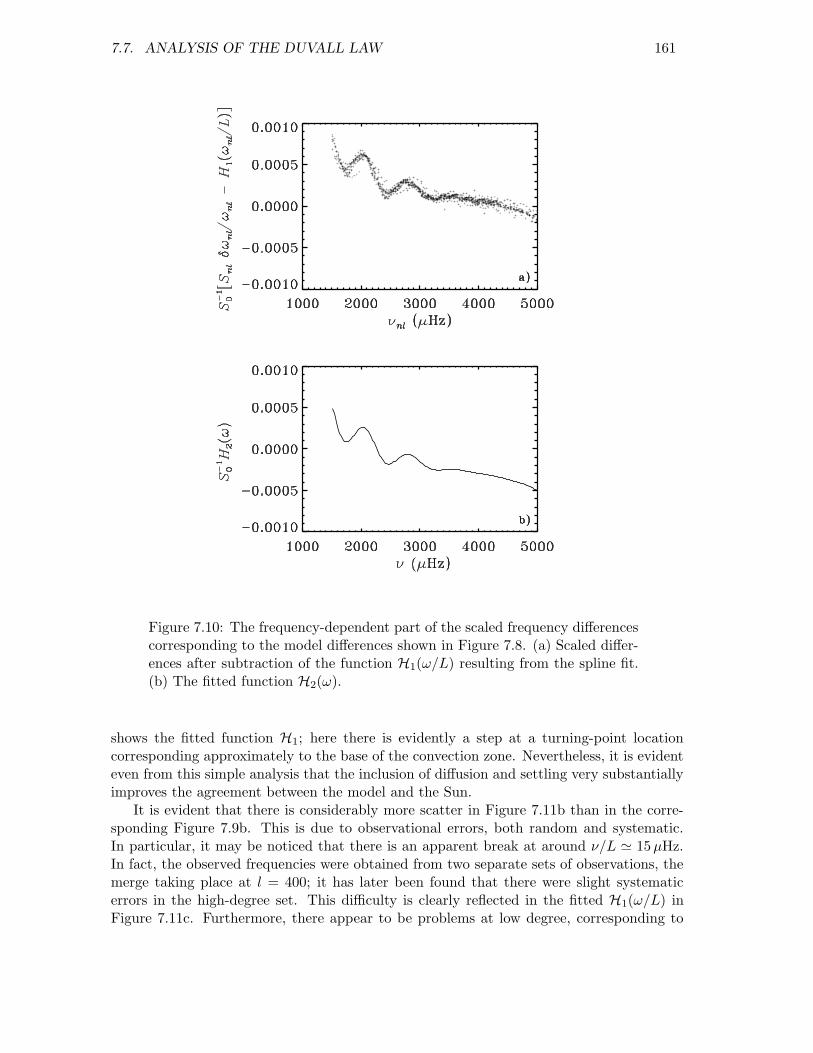
7.7. ANALYSIS OF THE DUVALL LAW 161
Figure 7.10: The frequency-dependent part of the scaled frequency differencescorresponding to the model differences shown in Figure 7.8. (a) Scaled differ-ences after subtraction of the function H1(ω/L) resulting from the spline fit.(b) The fitted function H2(ω).
shows the fitted function H1; here there is evidently a step at a turning-point locationcorresponding approximately to the base of the convection zone. Nevertheless, it is evidenteven from this simple analysis that the inclusion of diffusion and settling very substantiallyimproves the agreement between the model and the Sun.
It is evident that there is considerably more scatter in Figure 7.11b than in the corre-sponding Figure 7.9b. This is due to observational errors, both random and systematic.In particular, it may be noticed that there is an apparent break at around ν/L ' 15µHz.In fact, the observed frequencies were obtained from two separate sets of observations, themerge taking place at l = 400; it has later been found that there were slight systematicerrors in the high-degree set. This difficulty is clearly reflected in the fitted H1(ω/L) inFigure 7.11c. Furthermore, there appear to be problems at low degree, corresponding to

162 CHAPTER 7. ASYMPTOTIC THEORY OF STELLAR OSCILLATIONS
Figure 7.11: Scaled frequency differences between observed frequencies (seetext) and a solar model neglecting settling and diffusion, in the sense (obser-vations) – (model), plotted against ν/(l+ 1/2). The upper abscissa shows thelocation of the lower turning point, which is related to ν/(l + 1/2) throughequation (5.28). In panels (a) and (b) points corresponding to fixed l havebeen connected. (a) Original asymptotically scaled frequency differences. (b)Scaled differences, after subtraction of the function H2(ω) obtained from thespline fit. (c) The fitted function H1(ω/L).

7.7. ANALYSIS OF THE DUVALL LAW 163
Figure 7.12: Scaled frequency differences between observed frequencies (seetext) and a solar model including settling and diffusion, in the sense (obser-vations) – (model), plotted against ν/(l + 1/2). See caption to Figure 7.11.
the highest values of ν/L.The residual after subtraction of the fitted H1 from the scaled differences, and the fitted
H2, are shown in Figure 7.13. In panel (a) are shown the residuals for the model neglectingdiffusion and settling. As before, these are indeed predominantly a function of frequency.

164 CHAPTER 7. ASYMPTOTIC THEORY OF STELLAR OSCILLATIONS
Figure 7.13: The frequency-dependent part of the scaled frequency differencesbetween observations and models. (a) Scaled differences, shown in Figure7.11a, after subtraction of the function H1(ω/L) resulting from the spline fit.(b) The solid line shows the fitted function H2(ω) for this data set, whilethe dashed line shows the corresponding fitted function obtained from thedifferences in Figure 7.12a.
They are dominated by a slowly varying trend which, as argued in Section 7.7.3 belowreflects errors in the near-surface region of the model. However, there is also a weak butclearly noticeable oscillatory signal. As discussed in Section 7.7.3 this probably reflects adifference between the Sun and the model in the hydrogen abundance in the convectiveenvelope. This oscillatory behaviour is also very evident in the fitted H2(ω), shown as asolid line in panel (b). In contrast, H2(ω) for the model with settling and diffusion, shownas a dashed line, gives very little evidence for such oscillations, indicating that the envelopehydrogen abundance for this model is quite similar to that of the Sun.

7.7. ANALYSIS OF THE DUVALL LAW 165
7.7.2 Inversion of the Duvall law
The function F (w) in equation (7.143) can be determined from the observations (cf. Figure7.1). Given F , equation (7.144) is an integral equation of the Abel type, and can be invertedanalytically to obtain the sound speed implicitly, thus:
r = R exp
[− 2
π
∫ a
as
(w−2 − a−2
)−1/2 dF
dwdw
](7.152)
(Gough 1984). This relation was used by Christensen-Dalsgaard et al. (1985) to infer thesound speed in the solar interior. The properties of this inversion technique were discussedin considerable detail by Gough (1986b).
Exercise 7.5:
Confirm that equation (7.152) is a solution to equation (7.144). This is most simplydone by substituting equation (7.144) into equation (7.152).
The asymptotic description leading to equation (7.152) clearly suffers from systematicerrors. It has been found, for example, that for the most deeply penetrating modes of lowdegree the perturbation to the gravitational potential has a substantial effect on the func-tions F (ω/L) obtained by fitting the relation (7.143) to computed or observed frequencies;this may cause problems for the inversion in the solar core. Also, for modes trapped near thesurface the behaviour near the upper turning point depends on the degree; this introduceswhat is effectively an l-dependent term in α. It is possible to generalize equation (7.143) totake such effects into account and hence obtain a substantially more precise inversion (e.g.Vorontsov & Shibahashi 1991).
Alternatively, it appears that the systematic errors cancel to some extent when differ-ences are taken between inversions of different sets of frequencies. Christensen-Dalsgaardet al. (1985) made use of this by considering differences between inversions done for thesolar data and for frequencies for a reference model. A more systematic approach followsfrom the separation of scaled frequency differences in equation (7.147). Here the functionH1(ω/L) is related to the sound-speed difference between the models, or between the Sunand the model, through equation (7.148). As shown by Christensen-Dalsgaard, Gough &Thompson (1989), given a determination of H1, that equation is an integral equation forδrc/c, with the solution
δrc
c= −2a
π
d
d ln r
∫ a
as
(a2 − w2)−1/2H1(w)dw , (7.153)
where as = a(R). [It should be noticed that the right-hand side of equation (7.148) isthe same functional of w as that which arises in the asymptotic expression for the linearfrequency splitting due to latitudinally-independent rotation at a rate Ω(r), with δrc/cinstead of Ω (Gough 1984). Thus it can be inverted in the same way.]
Christensen-Dalsgaard et al. (1989) carried out a careful test of the differential method,as applied to several different pairs of models. Also, Christensen-Dalsgaard, Gough &Thompson (1988) used the method to invert differences between observed frequencies andfrequencies computed for a solar model. Here I illustrate its properties by applying it to the

166 CHAPTER 7. ASYMPTOTIC THEORY OF STELLAR OSCILLATIONS
Figure 7.14: The solid line shows the difference in squared sound speed δrc2/c2
inferred by applying equation (7.153) to the function H1(ω/L) shown in Fig-ure 7.9c. For comparison, the dashed line shows the true difference betweenthe two models. Adapted from Christensen-Dalsgaard, Proffitt & Thompson(1993).
model pair shown in Figure 7.8 and to differences between solar and computed frequenciessuch as those shown in Figures 7.11 and 7.12.
Figure 7.14 shows the δrc2/c2 inferred from the scaled frequency differences in Figure
7.9 between the diffusive and the normal solar model, by applying equation (7.153) to thefitted function H1(ω/L) shown in Figure 7.9c. For comparison, the figure also shows thetrue sound-speed difference, previously plotted in Figure 7.8. It is evident that the inversionreproduces the main features of the true δrc
2/c2 with considerable precision. One noticeabledifference is that the transition at the base of the convection zone is less sharp: as discussedin Section 9.1 it is a general property of inverse analyses that they smooth the properties ofthe true structure. However, otherwise the inferred and the true δrc
2/c2 are quite close overthe entire range, 0.2R < r < 0.95R, where the solution is plotted. At smaller and largerradii the systematic errors associated with the asymptotic representation increasingly affectthe results; hence here the solution has not been obtained.
From the frequency differences illustrated in Figures 7.11 and 7.12 we may now inferthe error in the sound speed in the solar models. Figure 7.15 shows the results of evaluatingδrc/c by applying equation (7.153) to the H1(ω/L) shown in Figures 7.11c and 7.12c. Thesound-speed differences are small, corresponding to errors in T/µ in the models of generallyless than 2 per cent. Nonetheless, the differences are clearly highly systematic. It is inter-esting that the relatively subtle, and often neglected, effect of gravitational settling leadsto a substantial improvement in the agreement between the model and the observations,largely by increasing the depth of the convection zone in the model. This is a strikingillustration of the power of helioseismology to probe the details of the solar interior. How-ever, it should also be pointed out that modest modifications in the opacity, well within the

7.7. ANALYSIS OF THE DUVALL LAW 167
Figure 7.15: The dotted line shows the difference in squared sound speedδrc
2/c2 between the Sun and a solar model without diffusion and settling,inferred by applying equation (7.153) to the functionH1(ω/L) shown in Figure7.11c, corresponding to differences between observed and model frequencies.The solid line shows the corresponding δrc
2/c2 between the Sun and a modelincluding diffusion and gravitational settling, obtained fromH1(ω/L) in Figure7.12c.
precision of current opacity tables, might introduce changes in the sound speed of similarmagnitude. The separation of opacity uncertainties from effects of diffusion and settlingis a major challenge, which will undoubtedly require better physical understanding of theprocesses involved.
The cause of the dominant difference between the Sun and the nondiffusive model isprobably that the depth of the convection zone in the model is too small. In fact, themodel with diffusion has a slightly deeper convection zone. From a more careful analysisof such results of inversions it is possible to obtain an estimate of the convection-zonedepth db which is largely independent of other uncertainties in the model. In this wayChristensen-Dalsgaard, Gough & Thompson (1991) found that db = (0.713± 0.003)R.
It should finally be mentioned that several other techniques have been developed to in-vert the Duvall law (7.143) (Brodsky & Vorontsov 1987, 1988a; Shibahashi 1988; Shibahashi& Sekii 1989). Gough & Thompson (1991) have made a comparison of these different tech-niques. The results suggest that, at least for the cases considered, the differential techniquedescribed here is superior. Nonasymptotic inversion of similar data sets will be discussedin Section 9.2.
7.7.3 The phase-function difference H2(ω)
The function H2(ω) is predominantly determined by the region near the stellar surface.Christensen-Dalsgaard & Perez Hernandez (1992) analyzed the relation of H2(ω) to thedifferences in sound speed and Γ1 in the outer parts of the Sun: differences localized very

168 CHAPTER 7. ASYMPTOTIC THEORY OF STELLAR OSCILLATIONS
near the surface give rise to a component ofH2 that varies slowly with ω, whereas differencesat somewhat greater depth introduce an oscillatory variation with ω in H2, the “frequency”of which increases with the depth of the difference. This is in fact a general property offrequency differences caused by sharply localized modifications to stellar structure (e.g.Thompson 1988; Vorontsov 1988; Gough 1990), and reflects the variation with frequencyin the phase of the eigenfunction at the location of the modification. At the surface thebehaviour of the eigenfunction changes slowly with frequency, whereas at greater deptha change in frequency causes the eigenfunction to “sweep through” the point where themodel was changed, causing a rapid variation in the frequency change. In the case of thevariation of H2 with ω, Christensen-Dalsgaard & Perez Hernandez (1991) found severalcases where the relatively sharp change in Γ1 in the second helium ionization zone causedan oscillatory behaviour of H2(ω). Similar variations in the basic phase function α(ω) wereanalyzed, for example, by Brodsky & Vorontsov (1988b, 1989) and Baturin & Mironova(1990). Vorontsov, Baturin & Pamyatnykh (1992) showed how the phase could be separatedin a quantitative fashion into components varying slowly and rapidly with frequency. Thistype of analysis provides a powerful diagnostic of the properties of the ionization zones ofhydrogen and helium, of great interest both for the analysis of the equation of state andfor attempts to determine the helium abundance of the solar convection zone.
It is very convenient to express H2(ω) in terms of differences between two models, orthe Sun and a model, in a form analogous to equation (5.90). Christensen-Dalsgaard &Perez Hernandez (1992) showed that α(ω), and hence H2(ω), can be determined directlyfrom the model structure, without computing full modes of oscillation. In this way theywere able to find kernels relating H2 to the model changes. The kernels turn out to beparticularly simple if the model changes are expressed in terms of c and the (isothermal)acoustical cut-off frequency
ωa =c
2Hp=
Γ1g
2c(7.154)
(cf. eq. 5.45). Thus I express H2 as
H2(ω) =
∫ R
r0
[Kc(r;ω)
δrc
c+Kωa(r;ω)
δrωa
ωa
]dr + G2(ω) , (7.155)
where r0 is a point suitably deep in the convection zone. Here, as in equation (5.90), theterm G2(ω) contains the contributions from the differences (or errors) in the physics of theoscillations: as argued in Section 5.5.3 such errors are likely to be confined very close tothe stellar surface and hence probably depend on frequency alone, when properly scaled.
The kernel Kc varies slowly with position and frequency, and hence give little interestingcontribution toH2. On the other hand, the kernels Kωa have a very distinct behaviour. Thisis illustrated in Figure 7.16, both as a function of r (at fixed frequency) and as a functionof frequency (at fixed r). The r-dependence is qualitatively similar to the behaviour of thescaled eigenfunctions shown in Figure 5.8: the kernels oscillate within an envelope whichvaries as c(r)−1. The frequency dependence clearly illustrates the behaviour discussedabove in a qualitative manner: at the surface the kernels vary slowly with frequency (theerratic variations at the lowest frequencies are due to numerical errors), and the variationwith frequency becomes increasingly rapid with increasing depth. In fact, as shown byChristensen-Dalsgaard & Perez Hernandez (1992) the kernels may be approximated by
Kωa(r;ω) ' − 1
c(r)cos[2ω(τ(r)− τ ′)] , (7.156)

7.7. ANALYSIS OF THE DUVALL LAW 169
Figure 7.16: The kernels Kωa(r;ω) relating changes in ωa to H2(ω) (cf. eq.7.155). The left-hand column shows the kernels as functions of r at the fre-quencies indicated, whereas the right-hand column shows the kernels againstfrequency, at the radii indicated.
where
τ(r) =
∫ R
r
dr
c(7.157)
is the acoustical depth, i.e., the sound travel time between the point considered and thesurface; also, τ ′ is roughly a constant. It is evident that according to equation (7.156) Kωa

170 CHAPTER 7. ASYMPTOTIC THEORY OF STELLAR OSCILLATIONS
is an oscillatory function of ω, oscillating increasingly rapidly with increasing τ and henceincreasing depth.
Figure 7.17: The adiabatic exponent Γ1 in a normal solar model (solid curve)and in a model with helium diffusion and settling (dashed curve).
Figure 7.18: Fractional differences between a model of the present Sun with dif-fusion and a normal model, without diffusion. The solid curve shows δrc
2/c2,the dashed curve δrΓ1/Γ1 and the dot-dashed curve δrωa/ωa (cf. eq. 7.154).
According to equation (7.155) the variation of Kωa with ω at a certain r correspondsto the H2(ω) arising from a localized change in ωa at that position. Hence a sharp featurein δrωa at some point r = r∗ will give rise to an oscillatory contribution to H2(ω) with a

7.7. ANALYSIS OF THE DUVALL LAW 171
‘frequency’ which, from equation (7.156), is approximately 2τ(r∗). Such contributions arein fact clearly visible both in Figure 7.10b, corresponding to the difference between twomodels differing in the envelope helium abundance, and in Figure 7.13b for the differencesbetween the Sun and a model. The ‘frequency’ of the variation corresponds to a depth ofroughly 0.02R, i.e., the region of the second ionization of helium.
To understand the origin of this feature I first consider the behaviour of Γ1. In regionsof no or full ionization it is very close to 5/3. However, ionization causes a decrease of Γ1
below this value; as illustrated in Figure 7.17, there is a major dip in Γ1 in the overlappingregions of hydrogen and first helium ionization and a smaller, secondary dip in the region ofsecond helium ionization. It is evident that the depth of the second dip must depend on thehelium abundance. The effect is clearly visible by comparing the solid curve in Figure 7.17,for the normal nondiffusive model with an envelope helium abundance Ye = 0.28, with thedashed curve for the model with diffusion and settling, where Ye has been reduced to 0.25.These effects are also evident in the differences between the two models, shown in Figure7.18 (the sound-speed difference was also shown in Figure 7.8, but for the whole model).In particular, there is a fairly sharp feature in δrωa at r ' 0.985R, which is responsible forthe oscillatory contribution to H2(ω) noted in Figure 7.10b.
These results suggest that H2 may provide useful information about the properties ofthe upper parts of the convection zone, including the solar envelope helium abundancewhich is otherwise quite uncertain. In fact, it was noted in Section 5.1.2 that the structureof the adiabatic part of the convection zone is determined by the composition, in particularthe value of Ye, as well as the specific entropy s which is essentially constant; in addition,the equation of state must be known. Indeed, the H2(ω) which results from the differencesbetween the observed and the computed frequencies (cf. Figure 7.13b) shows oscillationswhich are superficially quite similar to those resulting from the difference in Ye, althoughoverlayed by a substantial slowly varying trend. As shown by Figure 7.16, this slowlyvarying component approximately corresponds to the contributions that may arise fromdifferences in the outermost parts of the model. More generally, the uncertain physics inthe layers immediately below the photosphere and in the solar atmosphere may be expectedto give rise to a similar behaviour, as indicated by the function G2(ω) in equation (7.155).This complicates the interpretation of the H2(ω) determined from the observed frequencies.It was shown by Perez Hernandez & Christensen-Dalsgaard (1994a) that the slowly varyingpart of H2 can be suppressed in a consistent way through filtering. Furthermore, PerezHernandez & Christensen-Dalsgaard (1994b) made a fit of the resulting filtered H2 tomodels differing in Ye and s, as well as the surface properties; in this way they inferred thatYe = 0.243 ± 0.002. It might be noted that this is quite close to the value obtained in themodel with helium settling and diffusion.
The results of such fits, or more generally of any attempt to measure Ye from analysisof solar oscillation frequencies, depend critically on the equation of state. Indeed, all suchmethods utilize the variation of Γ1 in the ionization zones; this variation evidently dependson the details of the ionization processes and hence on the thermodynamic properties of theplasma. In fact, Perez Hernandez & Christensen-Dalsgaard (1994b) found that the qualityof the fit depended quite sensitively on the assumed equation of state, giving strong prefer-ence for one formulation over another, even though both were comparatively sophisticated.This indicates that it may be possible to get some separate information about the compo-sition and the thermodynamic properties of matter in the solar convection zone. However,it is evident that one might conceive of errors in the equation of state with an effect similar

172 CHAPTER 7. ASYMPTOTIC THEORY OF STELLAR OSCILLATIONS
to that corresponding to a change in the helium abundance. Such effects evidently cannotbe separated on the basis of an analysis of the oscillation frequencies.
I finally note that the function α(ω) also enters into the asymptotic behaviour of low-degree modes (cf. eq. 7.55); this is visible in the curvature, essentially similar for the differentdegrees, in the echelle diagram of low-degree solar observations in Figure 2.15. This sug-gests that it may be possible to obtain information about the near-surface regions, similarto what can be determined from H2(ω), by analyzing observations of stellar oscillationswhere only modes of degree less than three are generally visible. Brodsky & Vorontsov(1988a) presented a method to determine a function closely related to α(ω) on the basisof low-degree data alone. This was applied to models of main-sequence stars by PerezHernandez & Christensen-Dalsgaard (1993), who found a characteristic dependence on thestellar parameters. Further analyses of the effects on the frequencies or frequency separa-tions of the detailed properties of the helium ionization zones were carried out by Monteiro& Thompson (1998) and Miglio et al. (2003). A demonstration of the practical utility ofthis type of analysis, given realistic observational errors and other uncertainties, requiresmore extensive investigations, however.