R & D Report 1995:1. Asymptotic theory for order sampling / Bengt Rosén. Digitaliserad av Statistiska centralbyrån (SCB) 2016. urn:nbn:se:scb-1995-X101OP9501

INLEDNING

TILL

R & D report : research, methods, development / Statistics Sweden. – Stockholm :

Statistiska centralbyrån, 1988-2004. – Nr. 1988:1-2004:2.

Häri ingår Abstracts : sammanfattningar av metodrapporter från SCB med egen

numrering.

Föregångare:

Metodinformation : preliminär rapport från Statistiska centralbyrån. – Stockholm :

Statistiska centralbyrån. – 1984-1986. – Nr 1984:1-1986:8.

U/ADB / Statistics Sweden. – Stockholm : Statistiska centralbyrån, 1986-1987. – Nr E24-

E26

R & D report : research, methods, development, U/STM / Statistics Sweden. – Stockholm :

Statistiska centralbyrån, 1987. – Nr 29-41.

Efterföljare:

Research and development : methodology reports from Statistics Sweden. – Stockholm :

Statistiska centralbyrån. – 2006-. – Nr 2006:1-.

Asymptotic Theory for Order Sampling

Bengt Rosén

R&D Report Statistics Sweden

Research - Methods - Development 1995:1

Från trycket Mars 1995 Producent Statistiska centralbyrån, utvecklingsavdelningen Ansvarig utgivare Lars Lyberg

Förfrågningar Bengt Rosén tel 08-783 44 90 telefax 08-661 52 61

© 1995, Statistiska centralbyrån, 115 81 STOCKHOLM ISSN 0283-8680

Printed March, 1995 Producer Statistics Sweden Publisher Lars Lyberg

Inquiries Bengt Rosén telephone +46 08 783 44 90. telefax+46 8 661 52 61

© 1995, Statistics Sweden, S-115 81 STOCKHOLM, Sweden ISSN 0283-8680

February 1995

Asymptotic Theory for Order Sampling

Bengt Rosén

Abstract. The paper treats a particular class of sampling schemes, called order sampling schemes, which are executed as follows. Independent random variables, called ordering variables, are associated with the units in the population. A sample of size n is generated by first realizing the ordering variables, and then letting the units with the n smallest ordering variable values constitute the sample.

Although simple to describe and simple to execute, order sampling has an intricate theory. Standard results for linear estimators cannot be applied, since it is impossible to exhibit man­ageable exact expressions even for first order inclusion probabilities, and matters become only worse for second order quantities. These obstacles are circumvented by asymptotic considerations, which lead to approximation results. The instrumental tool is a general limit theorem for "passage variables". This result prepares for asymptotic results for linear statistic under order sampling. In particular, estimation issues are considered.

By altering the distributions of the ordering variables, a wide class of varying probabilities sampling schemes is obtained. At least two special cases have been considered in the litera­ture; successive sampling and sequential Poisson sampling. These sampling schemes are speci­fied, and their asymptotic theory is studied. Sequential Poisson sampling is, since 1990, used in the Swedish Consumer Price Index survey system.

CONTENTS Page

1 Introduction 1 1.1 Outline 1 1.2 Some notation 1

2 Order Sampling 2

3 Asymptotic Distributions for Linear Statistics Under Order Sampling 3 3.1 The main result in approximation version 3 3.2 The limit theorem 4 3.3 Estimation of population characteristics from an order sample 5

4 Asymptotic Results for Sequential Poisson and Successive Sampling 6 4.1 Sequential Poisson sampling 6 4.2 Successive sampling 6

5 A General Limit Result for Passage Variables 8 5.1 Some notation and terminology 8 5.2 A limit theorem for passage variables 9 5.3 Proof of Lemma 5.1 11

6 Proof of Theorem 3.1 12 6.1 The proof 12 6.2 Two auxiliary results 16

References 16

Asymptotic Theory for Order Sampling

1 Introduction 1.1 Outline

We consider probability sampling without replacement from a population U = {1, 2,.... N}. Inclusion probabilities are denoted by n{ = P(Ij = 1), i = 1, 2, ..., N, where I; is the sample inclusion indicator (= 1 if unit i is sampled, and =0 otherwise). A variable on U, x = (x1; x2,..., xN), associates a numerical value to each unit in U. A linear statistic is of the form (1.1), where the values of the variable a = (a^ a2,..., aN) are presumed to be known for all units in the population, while those of x = (xl5 x2,..., xN) are known only for sampled units;

(1.1)

A linear statistic of special interest is the Horvitz - Thompson (HT) estimator x(x)HT, which is obtained by setting aj = 1/K{ in (1.1). x(x)HT yields unbiased estimation of the population total t(x) = X!+ x2+ ...+ xN. The literature provides formulas, in terms of first and second order inclusion probabilities, for the theoretical variance of ^(x)^ as well as for variance estimators.

This paper treats a particular class of sampling schemes, called order sampling schemes, which are executed as follows. With the units in the population are associated independent random variables; ordering variables. A sample of size n is generated by first realizing the ordering variables, and then letting the units with the n smallest values constitute the sample.

Although order sampling is simple to describe and simple to execute, its theory is intricate. Standard results for linear estimators cannot be applied, since it is impossible to exhibit man­ageable expressions even for first order inclusion probabilities, and matters become only worse for second order quantities. To circumvent these obstacles we follow an asymptotic considerations route, which leads to approximation results. The instrumental tool in the con­siderations is a general limit theorem, which is proved in Section 5. Based on this theorem, asymptotic results for linear statistic under order sampling are formulated in Section 3, and proved in Section 6. In particular, estimation issues are treated in Section 3.3.

By varying the distributions of the ordering variables, a wide class of varying probabilities sampling schemes is obtained. At least two special cases have been considered in the litera­ture; successive sampling and sequential Poisson sampling (SPS), which correspond to expo­nential respectively uniform ordering distributions. These sampling schemes are specified in Section 2, and further treated in Section 4. Successive sampling with small sample sizes is considered in most sampling books, see e.g. Cochran (1977), Section 9A.6. Asymptotic results for successive sampling have been studied by i.a. Rosén (1972) and Hâjek (1981). Sequential Poisson sampling is, since 1990, used in the Swedish Consumer Price Index survey system, see Ohlsson (1990). Ohlsson (1995a) shows that SPS provides a mean for coordination of pps-samples by permanent random numbers. The investigations which are reported in this paper were initiated by discussions with Dr. Ohlsson on SPS problems. SPS will, however, not be treated in depth here, since a special study of it is presented in Ohlsson (1995b). As regards applications, we presume that other order sampling situations may be encountered in practice, perhaps not as a result of an imposed sampling scheme, but because "nature" sampled in this way.

1.2 Some notation

Here we list some notation which will be used throughout the paper.

Arithmetic operations on (population) variables shall be interpreted component-wise, e.g. for x = (x1,x2)...,xN)andy = (y1,y2,...,yN),weletx-ymean(x1-y„...,xN-yN).

1

A standardized version of a general linear statistic is given by the sample sum statistic. When the variable is z = (z]5 z2,..., zN) and the sample size is n, it is denoted by S(n;z);

(1.2)

Remark 1.1: The relation

(1.3)

shows that a linear statistic can be viewed as a sample sum. In particular; T(X)H T= S(n; a/n). With (1.3) as background, most of the following results will be formulated in terms of sample sums, although the main interest concerns more general linear statistics. •

Finally some probability notation. P, E and Var denote probability, expected value and vari-

ance, and c stands for centering at expectation, i.e. Zc = Z - EZ. —» denotes convergence in probability, and => convergence in distribution (or synonomously in law). N(p.,a2) denotes the normal distribution with mean jx and variance a2.

2 Order Sampling

DEFINITION 2.1: Order sampling with sample size n and ordering distribution functions F = (F1; F2,..., FN), denoted OS(n; F), is carried out as follows. Independent non-negative random variables Q,, Q2,..., QN with absolutely continuous distributions F on [0,°°) are associated with the units in the population U = {1,2,...,N}, Q{ with unit i. The Q:s are realized, and the units with the n smallest Q-values constitute the sample. The densities of the ordering distributions are denoted (f,, f2,..., fN).

Since the ordering distributions are continuous, the realized Q-values contain (with probability 1) no ties. Hence, the sample has fixed size n. If all ordering distributions are equal, OS(n; F) is simple random sampling, for which the population units have equal inclusion probabilities. However, as soon as all F; are not equal, OS(n; F) has non-equal inclusion probabilities. By varying the ordering distributions, OS(n; F) generates quite a wide class of varying probabilities sampling schemes, two of which are specified below.

DEFINITION 2.2: a) Sequential Poisson sampling is order sampling with uniform ordering distributions. For 6=(6,,62,..,6N), fy >0, SPS(n;6) stands for OS(n;F) with Fj = the uniform distribution on [0, l/GJ, i = 1,2, ...,N.

b) Successive sampling is order sampling with exponential ordering distributions. For 6 = (9i, 62,.., 0N), Q{ > 0, SUC(n; 0) stands for OS(n; F) with;

(2.1)

Remark 2.1: For elaborate discussions of SPS, we refer to Ohlsson (1990, 1995a and b). •

Remark 2.2: Definition 2.2.b of successive sampling is not the usual one, which runs as fol­lows. The sample is generated sequentially by n successive draws without replacement. As long as unit i remains in the population U, it is, at each draw, selected among remaining units, with probability proportional to 6,. The probability for selection of the ordered sample (i,. i2, ..., i ) of different units from U is then, t(6) = 6,+9„, +...+6„ ;

(2.2)

Next we show that Definition 2.2.b also leads to (2.2), with sample order by increasing

Q -values. First some preparations. For X > 0, Exp(Å.) denotes the distribution with density

2

k • exp(- X • t), t > 0. In (i) - (iii) we list well-known properties of independent random variables X and Y with Exp(A,x) and Exp(Xy) distributions respectively, (i) min(X,Y) is Exp^+Ày). (ii) P(X< Y) = Xx/(kx+Xy). (iii) For a random T which is independent of X and Y, the conditional distribution of X and Y given that X > T and Y > T, is the same as the unconditional distribu­tion ("X and Y have no memories").

In the verification of (2.2), we confine to n = 2, which suffices to indicate the general principle. Let j and k be different units in U, and let p(j,k) = P(Qj and Qk are the two smallest Q-values, and Qj<Qk). The following relation (2.3) holds for order sampling in general;

(2.3)

The variables Q, and min{Qj ; i=j} are independent. Under (2.1) Qj is Exp(6j) and, by (i), minfQ; ; i=j} is Exp(t(6) - fy). Hence, by (ii), the left hand factor in (2.3) is 6/1(6). As regards the right hand factor, first note that, by (iii), it equals the corresponding unconditional prob­ability, then argue as before. The variables Qk and minfQ; ; i=j,k} are independent, Qk is Exp(6k) and, by (i), min{Qi;i=j,k} is Exp(T(e)-er6k). Hence, by (ii), P(Qk<min{Qi;i^j,k}) = 6k/(x(6)-6j). Thereby relation (2.2) is obtained (for n=2). •

3 Asymptotic Distributions for Linear Statistics Under Order Sampling

In this section we consider limit results for linear statistics under order sampling. The practical interest in such results stems from the fact that they lay ground for approximations, which can be employed in practical, "finite" situations. We high-light this aspect by formulating approximation results as well as stringent limit results. The latter provide justification of the former and, moreover, the conditions for the validity of a limit result shed light on the question when a corresponding approximation can be expected to be "good enough". In the first two subsections we confine to the standardized linear statistic, the sample sum. In Section 3.3, which treats estimation issues, we illustrate the statement in Remark 1.1, that results about sample sums readily are transformed to results for general linear statistics.

3.1 The main result in approximation version

APPROXIMATION RESULT 3.1: Consider OS(n;F) from U=(1,2,...,N). Let z = (z„z2,

..., zN) be a variable on U, and S(n;z) the corresponding sample sum. Then, with \i and a as specified below, the following holds under general conditions;

Law[S(n; z)] is well approximated by N(^i,a2). (3.1)

Specification of parameters

(3.2)

(3.3)

(3.4)

(3.5)

(3.6)

3

The sum of distribution functions in (3.2) is non-decreasing, as t increases. The formula (3.4)

tacitly presumes that its derivative £ $(£) is positive in t = Ç, which we make to a formal

assumption. Then, the solution to (3.2) is unique. •

3.2 The limit theorem

THEOREM 3.1: For k = 1,2,..., an OS(nk; Fk) sample is drawn from Uk = (1,2,..., Nk). The density for Fki is denoted by fki. Let zk = (zkl, zk2,..., zkNk ) be a variable on Uk and

Sk(nk; zk) be the corresponding sample sum. Define £k, jxk, <j)k and ak in accordance with H.2W3.5Ï. Then.

(3.7) provided that conditions (B1)-(B5) below are satisfied.

(Bl)

(B2)

(B3)

(B4) For some 8>0, some C<°° and some function w(A) which tends to 0 as A—»0, the following inequalities hold for l-ô< t,s< 1+5;

(3.8)

(B5) For some p>0, we have;

(3.9)

Proof of the theorem is given in Section 6.

Remark 3.1: The contents of condition (B2) is that no zki -value is allowed to deviate "extremely" from the majority of z^ -values. (B2) is somewhat involved, though, to the effect that it depends on the ordering distributions as well as on the zkj. A related condition, which pays regard only to the spread of the zu -values, is Noether's condition (N), which is stated below. Let zk and co denote the "ordinary" population mean and population variance;

(3.10)

Introduce the following conditions;

(N)

(B6)

(B7)

Then the following implications hold;

(3.11)

(3.12)

Verification: For any Xi,X2e [min; z^ , maXj z^ ]; max; | zki - X\ \ <2 • max; jz^ - X,2|. Since <j)k

and zk both e [min; z^, max; zki] (cf. (3.4) and (3.10)), we have

(3.13)

4

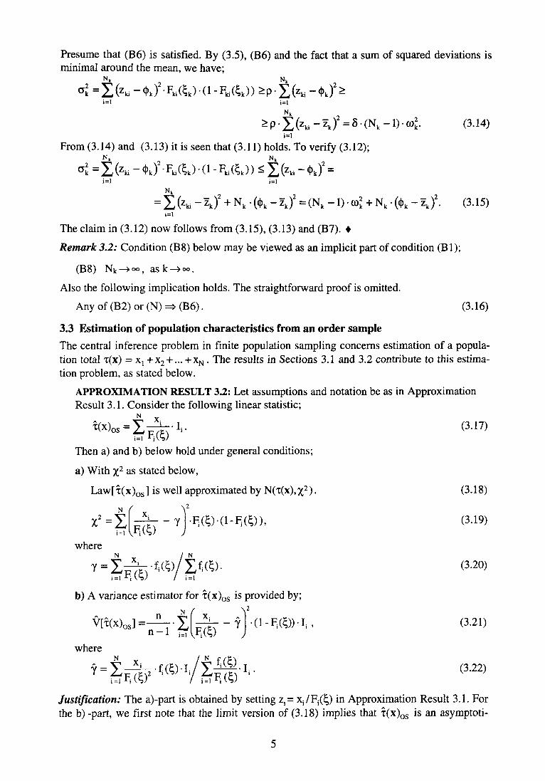
Presume that (B6) is satisfied. By (3.5), (B6) and the fact that a sum of squared deviations is minimal around the mean, we have;

(3.14)

From (3.14) and (3.13) it is seen that (3.11) holds. To verify (3.12);

(3.15)

The claim in (3.12) now follows from (3.15), (3.13) and (B7). •

Remark 3.2: Condition (B8) below may be viewed as an implicit part of condition (Bl);

(B8) Nk->°°, ask->°o.

Also the following implication holds. The straightforward proof is omitted.

Any of (B2) or (N) => (B6). (3.16)

3.3 Estimation of population characteristics from an order sample

The central inference problem in finite population sampling concerns estimation of a popula­tion total T(X) = X! +x2 + ... +xN . The results in Sections 3.1 and 3.2 contribute to this estima­tion problem, as stated below.

APPROXIMATION RESULT 3.2: Let assumptions and notation be as in Approximation Result 3.1. Consider the following linear statistic;

(3.17)

Then a) and b) below hold under general conditions;

a) With x2 as stated below,

Law[x(x)os] is well approximated by N(x(x),x2). (3.18)

(3.19)

(3.20)

b) A variance estimator for î(x)o s is provided by;

(3.21)

(3.22)

Justification: The a)-part is obtained by setting z;= Xj/F;(!;) in Approximation Result 3.1. For the b) -part, we first note that the limit version of (3.18) implies that î(x)os is an asymptoti-

5

cally unbiased estimator of x(x). By combining this with the fact that the HT-estimator x(x)m

is unique as unbiased linear estimator of T(X), one is led to the conjecture that good approxi­mations of OS(n;F) inclusion probabilities, under general conditions are given by;

(3.23)

The justification of the variance estimator (3.21) is heuristic to the effect that it relies on (3.23) being a good approximation. In the first round, disregard the factor n/(n-l) in (3.21) and replace y by y. By taking expectation in (3.21), using (3.23) as an exact relation, and com­paring the result with (3.19), it is seen that V(T(X)) yields (formally) unbiased estimation of X2. However, in a practical situation y is not known, but has to be estimated. By using (3.23) as an exact relation again, it is seen that the denominator and nominator in (3.22) yield (formally) unbiased estimation of the corresponding quantities in 7 in (3.20). Hence, y is a natural estimator of 7. The factor n/(n-l), finally, is inserted on the following ground. In order that (3.21) should yield the standard SRS variance estimator when all Ft are equal, the adjustment factor n/(n-l) is needed. Based on simulations, Rosén (1992), we know that the adjustment works well in many successive sampling situations, and we conjecture that it is good also for general order sampling. •

4 Asymptotic Results for Sequential Poisson and Successive Sampling

Here we specialize the results in Sections 3.1 and 3.2 to sequential Poisson and successive sampling (see Definition 2.2. The parameter 8 = (9j,62,.., 8N) is said to be normalized if e1+e2+..+eN=i. 4.1 Sequential Poisson sampling

Since a study of SPS is presented in Ohlsson (1995b), we are brief on this topic, and we con­fine to specializing Approximation Result 3.1.

APPROXIMATION RESULT 4.1: Consider SPS(n; 8) from U = (1, 2,..., N), with nor­malized 6. Assume that n • 8; < 1, i = 1,2,..., N. Let z be a variable on U and S(n; z) the corresponding sample sum. Then (3.7) holds with the following JJ, and a;

(4.1)

(4.2)

Derivation from Approximation Result 3.1: By Definition 2.2, SPS(n; 8) is OS(n; F) with F;(t) = min(t • 8; ,1), and fs(t) = 8; on te [0,1/ej and =0 outside [0,1/6;], 0<t<°°, i= 1,2,...,N. On the interval 0<t<l/maxi8 i , all f;(t) are continuous, and (3.2) takes the form t ( 8 1 + 8 2 + ..+ 8N ) = 1, which under normalized 8 yields Ç=n. When n • 6j < 1, i = 1,2,..., N, £=n in fact lies on the interval (0, l/max; Q{). It is readily checked that (3.3) and (3.5) here specialize to (4.1) and (4.2). •

4.2 Successive sampling

Here we specialize the limit theorem as well as the approximation result.

APPROXIMATION RESULT 4.2: Consider SUC(n; 8) from U = (1, 2,...,N), with nor­malized 8. Let z be a variable on U and S(n; z) the corresponding sample sum. Then

(3.7) holds with |i and cr as stated below;

6

N

% is the solution to the equation (in t) £ ( 1 -e~6' ')= n. (4.3) i=l

VI

(4.4)

(4.5)

(4.6)

Derivation from Approximation Result 3.1: It is readily checked that (3.2) - (3.5) specialize to (4.3) - (4.6) when, see (2.1), F;(t) = l-e~9i ' and ii(t) = Qi- e~M, 0<t<°°. •

THEOREM 4.1: For k= 1,2,3,..., consider SUC(nk;0k) from Uk=(l,2,...,Nk), with nor­malized 0k. Let zkbe a variable on Uk and Sk(nk;zk) the corresponding sample sum. Let

£k, |ik, <t)k and ok be in accordance with (4.3) - (4.6). Then (3.7) holds, if conditions (C1)-(C4) below are satisfied.

Remark 4.1: The above theorem improves results in Rosén (1972) and Hâjek (1981), to the

effect that the conditions for asymptotic normality are more general. •

Remark 4.2: Here we comment on condition (C4). When the 6:s are normalized, the average

9^-value is 1/Nk. Say that 9U is "small" if 6ki<p/Nk (for some "small" p), otherwise say that it

is "non-small". (C4) requires that the number of non-small 9 is at least a bit larger than the

sample size and, moreover, that the non-small 9 comprise a non-negligible proportion of all 9.

Below we list some conditions which relate to (C4);

(C5) Forsomep>0; Qta> p/Nk, i=l,2,...,Nk, k=l ,2 ,3, . . . .

(C6) For some X<1; nk<A,-Nk, k= 1,2,3,....

The following implications hold;

(4.7)

(4.8)

To realize (4.7), presume that (C4) holds. Then, Nk>#{i: 0,, >p/Nk} >max(y- nk, Ô• Nk} > y- nk, from which (4.7) follows. To realize (4.8), presume that (C5) and (C6) hold. Then, #{i:9ki>p/Nk} =Nk> (by (C6))>max(X"' -nk,Nk}. Hence (C4) is satisfied. •

Proof of Theorem 4.1: We shall show that (CI) - (C4) imply (Bl) - (B5) in Theorem 3.1, which then yields Theorem 4.1. Set,

7

(4.9)

To estimate cp from above, use the inequality 1-e "<x, 0 < x < °° ;

(4.10)

Next we estimate cpk from below. Set Ak = #{i: e ^ p / N J . By (4.9) and (C4) we have;

(4.11)

Since <$\i) < (pk(t) < (p(ku)(t), and £k is the solution to %(t) = 1, £k lies between the solutions to

(p(ku)(t) = 1 and (pk°(t) = 1, which yields (4.12) below, where we also use ln(l-x)"1 <x/(l-x).

(4.12)

As a consequence of (C3) and (4.12), we have, for some C<°°;

(4.13)

We now turn to verification of (Bl) - (B5). (Bl) and (CI) are the same, and so are (B2) and (C2). (B3) is a consequence of the following two estimates, which hold when 6 is normalized;

(4.14)

(4.15)

(4.16)

From (4.16) and (4.13) it is seen that (B4) is satisfied. To verify (B5), finally, we use the in­equality l - e " x > x ( l - e _ x ° ) / x 0 , 0< x < x0, in combination with (4.13);

Thereby the theorem is proved. •

5 A General Limit Result for Passage Variables 5.1 Some notation and terminology We start by settling some notation and terminology to be used in this section. Let [t0,t,], t0<t1, be a specified interval, and z(t) a function on [t0, t,]. M(z) denotes the supremum of | z(t) | on [tn,t,]. The modulus of variation for z on rtn,t,l, w(A; z), is;

(5.1)

A sequence {zk(t)}~=1 of functions on [t0 , t,] is equicontinuous if there is a function w(A),

A > 0, with w(A) -> 0 as A -> 0, such that w(A; zk) < w(A), 0 < A < tj -10, k= 1,2,3,... . A sequence lQkJk=1 °f random variables is bounded in probability, if supk P(|Qk| > M) —> 0, as M —» °o. A

sequence {Zk}~=1 of stochastic process on [t0,t,] satisfies condition (T) if;

(5.2)

8

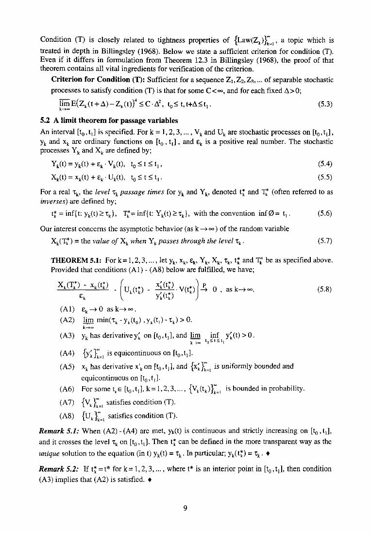
Condition (T) is closely related to tightness properties of {Law(Zk)}~=], a topic which is

treated in depth in Billingsley (1968). Below we state a sufficient criterion for condition (T). Even if it differs in formulation from Theorem 12.3 in Billingsley (1968), the proof of that theorem contains all vital ingredients for verification of the criterion.

Criterion for Condition (T): Sufficient for a sequence Z1.Z2.Z3,... of separable stochastic

processes to satisfy condition (T) is that for some C<°o, and for each fixed A>0;

(5.3)

5.2 A limit theorem for passage variables

An interval [t0,tj] is specified. For k = 1,2,3,..., Vk and Uk are stochastic processes on [ t 0 , t j , yk and xk are ordinary functions on [t0, t , ] , and ek is a positive real number. The stochastic processes Yk and Xk are defined by;

(5.4)

(5.5)

For a real Tk, the level Tk passage times for yk and Yk, denoted t£ and Tk* (often referred to as inverses) are defined by;

(5.6)

Our interest concerns the asymptotic behavior (as k —> °° ) of the random variable

(5.7)

THEOREM 5.1: For k= 1,2,3,..., let yk, xk, ek, Yk, Xk, xk, t and Tk* be as specified above. Provided that conditions (Al) - (A8) below are fulfilled, we have;

(5.8)

Remark 5.1: When (A2) - (A4) are met, yk(t) is continuous and strictly increasing on [t0 , t ,] ,

and it crosses the level xk on [t0 , t j . Then t* can be defined in the more transparent way as the

unique solution to the equation (in t) yk(t) = t k . In particular; yk(t*) = Tk. •

Remark 5.2: If t* =t* for k= 1,2,3,..., where t* is an interior point in [t0,t,], then condition (A3) implies that (A2) is satisfied. •

9

Remark 5.3: A main aspect on the result (5.8) is that it tells that the two terms have the same asymptotic behavior. As a consequence, a limit result for one of the terms holds also for the other. Usually, the term within brackets is simplest to study, and it provides a mean for study­ing the other term. This use of (5.8) is illustrated in Section 6. •

The crucial part of the proof of Theorem 5.1 is stated in the following Lemma 5.1, where we continue to use notation and assumptions as in Theorem 5.1. The situation in Lemma 5.1 is, however, more special. It concerns just one k -situation, and we omit the index k. Moreover, also V and U are presumed to be ordinary (= non-random) functions. Hence, in Lemma 5.1 Y, X, y, x, V and U are real-valued, bounded functions on an interval [^, t,], XQ < tl5 which are

related in accordance with (5.4) and (5.5), e and x being real numbers, e > 0. The level x passage times for y and Y, t* and T*, are defined in accordance with (5.6). Furthermore, we assume that the following counterparts to (A2), (A3) and (A5) are in force;

y(t0)<T<y(t1), (5.9)

The functions y and x have continuous derivatives y' and x' on [to.tj . (5.10)

For some m>0, y'(t)>m>0, to<t<t , . (5.11)

The proof of the following Lemma 5.1 is deferred until the next sub-section.

LEMMA 5.1: Let notation be as stated above. Assume that (5.9) - (5.11) are in force. Define

c by (5.12), and presume that e>0 is small enough for (5.13) and (5.14) to hold;

(5.12)

(5.13)

(5.14)

For R(e) as defined implicitly below, (5.16) then holds;

(5.15)

(5.16)

Remark 5.4: If we add to the other conditions in Lemma 5.1 that also U and V are continuous on [t0,tj], the bound in (5.16) tells that R(e)—>0 as £—>0. Hence, the remainder term e • R(£) in (5.15) becomes negligible as e tends to 0. •

Proof of Theorem 5.1: Set, in accordance with (5.15);

(5.17)

(A2), (A3) and (A5) imply that there arep>0, m > 0 M < °°, and 1^ < «>, such that;

(5.18)

Fix a ô>0. From (A6) and (A7) we conclude that there is a B5<oo, and a kj(5)<<», such that;

(5.19)

Set, in accordance with (5.12);

(5.20)

By virtue of (Al) and (A4) we have for some k2(ô) <°° ;

10

(5.21)

By (Al) and the left inequality in (5.18), the following bound holds on the set {|M(Vk)|)<B8} for some k,(8)<°o;

(5.22]

From (5.21) and (5.22) it is seen that Lemma 5.1 applies on the set {|M(Vk)|<B5} for k suffi­ciently large. Hence, by (5.16);

holds on {|M(Vk)|<B8}, fork>max{k0,k1(8),k2(8),k3(5)}. (5.23)

By (Al), (A4) and (A5), the two first terms in (5.23) tend to 0 as k ->°°. By (A7), (A8) and the definition of condition (T), the two last terms vanish on the set {|M(Vk)| <B5} as k —>°°. By (5.19), {|M(Vk)| <BS} has probability > 1 - 8. Hence, for every fixed 7>0, lim P(|Rk(ek)| > y) < 8. Since 8 is arbitrary, the claim in the theorem follows. •

5.3 Proof of Lemma 5.1 First we list a well-known result concerning Taylor approximation. (5.24) introduces a nota­tion for the remainder term in a one-step Taylor expansion. (5.25) presents an estimate of it, which follows from the mean value theorem. As before, w denotes modulus of variation.

(5.24)

(5.25)

Next we prepare the proof of Lemma 5.1 with two auxiliary lemmas.

LEMMA 5.2 Let notation and assumptions be as in Lemma 5.1. Then;

(5.26)

Proof: By (5.10), (5.11) and (5.9), y is continuous, strictly increasing, and crosses the level % on the interval [ t 0 , t j . Hence, t* is the unique solution to the equation y(t) = x. In particular;

(5.27)

(5.28)

(5.29)

By setting h = e • c in (5.29) and recalling (5.12), it is seen that Y(t*+ £ • c) > x, provided that t*+ e • c<ti. It may happen, though, that t*+ £ • c>ti. If so, note that Y(ti) = y(ti) + £ • V(t0 and (5.14) imply that Y(tj)>T. All in all this implies that Y(min(t*+£ • c, tj))>T.

By very similar reasoning, it can be shown that Y(max(t* - £ • c, t0)) < %. Hence, Y has a level T passage on the interval [max(t*-£-c, t0),min(t*+£-c,tl)], which is included in t* ± E • c. Thereby (5.26) is proved. •

11

LEMMA 5.3: Let notation and assumptions be as in Theorem 5.1, and define Q(e) by (5.30). Then (5.31) holds.

(5.30)

(5.31)

Proof: Since Y need not be continuous nor increasing on [t0 .tj], Y(T*) and x are not as simply related as y(t*) and %. An analog to (5.27) is stated in (5.32), where w(0+ ; z) denotes the limit of w(A ; z) as A—>0, which also can be interpreted as the maximal jump for z on [t0,tj].

(5.32)

(5.33)

Rearrangement in (5.33), (5.27) and comparison with (5.30) yields;

(5.34)

By applying (5.32), (5.25) and (5.26) in (5.34), we get;

(5.35)

By using (5.26) and w(0+ ; z) < w(A ; z) in (5.35), the bound (5.31) is obtained. •

Proof of Lemma 5.1:

(5.36)

Insertion of T* -t* according to (5.30) into (5.36) and comparison with (5.15) yields;

(5.37)

By employing (5.25) in (5.37) we get

(5.38)

Now, application of (5.31) and (5.26) in (5.38) leads to (5.16). •

6 Proof of Theorem 3.1

6.1 The proof

The instrumental tool in the proof will be Theorem 5.1, and we start with some preparations for its application. For the ordering variables Q,, Q2,..., QN in Definition 2.1, introduce the following stochastic processes H;(s) on 0 < s < °°, where H; "counts when Q; occurs". ( 1A

denotes the indicator of the set A);

(6.1)

Hj(s) is a 0-1 random variable with expected value F;(s), which yields;

(6.2)

Define the stochastic processes J(t) and L(t;z) as follows, where z=(z,, z2..., zN) are given real numbers and ^>0 is arbitrary (but fixed);

(6.3)

Let T* be the time when J(t) hits the level n, and A(n; z) the value of L(t;z) at the hitting time;

12

(6.4)

The following relation (6.5) should be evident upon some thought. It provides the link between order sampling and passage variables, which allows application of Theorem 5.1.

The sample sum S(n; z) under OS(n; F) has the same distribution as A(n; z). (6.5)

We adhere to the sequence version in Theorem 3.1. For k= 1,2,3,.., let Jk(t), L^tjzJ, T* and

Ak(nk; zk) be in accordance with what is said above, and let Çk, |j,k, <|)k and ak be in accordance with (3.2) - (3.5). By virtue of (6.5) we have;

(6.6)

As will be proved, Theorem 5.1 yields that (Ak(nk; zk) - fik)/ok is asymptotically N(0,1) - dis­tributed under the conditions in Theorem 3.1. Having shown that, (6.6) tells that the same holds for (Sk(nk;zk) -|ik)/ak, and Theorem 3.1 is thereby proved.

When employing Theorem 5.1, the entities Yk, Xk, xk, yk,Vk, Uk, £k and tk are chosen as stated below. [t0,tj] = [1-5,1+0], where ô is that in (B4). When checking (6.7)-(6.10), recall the left equality in (6.2), and thatc = centering at expectation.

(6.7)

(6.8)

(6.9)

(6.10)

(6.11)

(6.12)

From (6.12) and (3.6) follows that tj in (5.6) here takes the value t£ = 1.

The proof of Theorem 3.1 comprises two main parts, which are stated as separate lemmas below. Together the two lemmas yield that ( Ak(nk; zk) - (ik)/Gk is asymptotically N(0,1)-distrib­uted under (Bl) - (B5), which is the claim in Theorem 3.1. In addition, Section 6.2 contains two lemmas with auxiliary results, which will be used in the sequel.

LEMMA 6.1: Under conditions (B1)-(B5) in Theorem 3.1, we have;

(6.13)

LEMMA 6.2: Under condition (B2) in Theorem 3.1, we have;

(6.14)

Proof of Lemma 6.2: Since Qkl,Qk2> ->QkN a r e independent, so are the processes Hki(t), i= 1, 2,...,Nk. Hence, cf. (6.10),

(6.15)

13

is a sum of independent random variables with means 0. By using (6.2) and (3.5) it is readily checked that the variance of Uk(l) is 1. To verify (6.14) we apply Lyapunov's condition, in 4:th moments version, for the central limit theorem for independent variables.

>. A . . .

.(6.16)

By (B2) the last term in (6.16) tends to 0 as k ->°o, and Lemma 6.2 is proved. •

Proof of Lemma 6.1: First we derive expressions for the two terms in (5.8). By (6.3) and (6.4), it is readily checked that;

(6.17)

Furthermore, (6.10), (3.3) and (3.4) yield;

(6.18)

From (6.17) and (6.18) we get;

(6.19)

The formulas for yk and xk in (6.8) and (6.10), and the assumption that the F^ have densities imply that yk and xk are differentiable on [t0 ,t,], and;

(6.20)

(6.21)

From (6.21) and (3.4) follows that x'k(t*)= x'k(l) = 0. Hence, the term to the right in (5.8) "collapses" to Uk(l). This together with (6.19) yields that if Theorem 5.1 applies in the present situation, it leads to (6.13). It remains, though, to show that Theorem 5.1 in fact does apply, which we do by proving that conditions (B1)-(B5) imply (A1)-(A8).

(Al) follows from (6.11) and (Bl). (A3) is the left part of (B3). By Remark 5.2, (A2) follows from (A3), tj = 1, k= 1,2,.., and the choice of the interval [t0 ,t,]. To verify (A4) we use (6.20);

(6.22)

Formula (6.22), the right hand part of (B3) and the properties of w yield that (A4) is satisfied. When considering (A5), we first show that {xk(l)}~=1 is bounded, and we start from (6.21).

(6.23)

By (3.5), the left square root in (6.23) equals 1. By using (B5) in the right hand square root, we

arrive at the following estimate, which together with (B3) shows that {xk(l)}~ is bounded;

14

(6.24)

Next we show that {xk(t))°°=] is equicontinuous on [to.tj, and we start from (6.21);

(6.25)

By (B3), (6.25) tells that {xk(t)}~=1is equicontinuous on [to.tj]. This together with {x'k(l)}^=1

being bounded verifies (A5). The following estimate implies (A6) (recall (6.8), (6.2) and (3.6));

(6.26)

To show that (A8) is met, we employ condition (5.3), and we start from (6.10);

(6.27)

Here we make an interlude to derive some auxiliary results.

(6.28)

(6.29)

Check: Recall that Fkj is differentiable with continuous derivative fki. By the mean value theo­

rem; | Fki(t • Çk) - Fki(s • Çk) | = 11 - s | • Çk • fki(K), where K is intermediate to t • ^ and s • ^ . By

applying first (6.28) and then (3.9), (6.29) is obtained.

We now return to (6.27). Note that HJt • £k) - H^s • £k) is a 0 -1 random variable with mean

value Fu(t • £k) - Fki(s • £j. By Lemma 6.3 and (6.29), (6.27) can be continued as follows;

(6.30)

15

By (3.5) the sums in (6.30) equal 1. From this and (B2) it is seen that the first term in (6.30) equals 0, and the second equals 6 • C " • (t - s)2. Now condition (5.3) tells that (A8) is satisfied. Verification of (A7) is similar but simpler, and some details are omitted. We start from (6.8);

XI

(6.31)

Now the estimate (6.31) together with (3.6) yields that (5.3) is satisfied, and (A7) is verified.

Hence, Lemma 6.1, and thereby also Theorem 3.1 are proved. •

6.2 Two auxiliary results

The following results are certainly known, but they are proved for the sake of completeness.

LEMMA 6.3: For a 0 -1 random variable Z with P(Z = 1) = p, we have;

(6.32)

Proof: By binomial expansion of (Z - p)4 and use of EZ = EZ2 = EZ3 = EZ4 = p, it follows that E(Zc)4=p.( l-p) .(3p2-3p+l)<p-(l-p)/4.4

LEMMA 6.4: Let Zj, Z2,..., ZN be independent random variables. Then;

(6.33)

Proof: By binomial expansion of ( ^ Z\ )4 = ( Z^ + Z£, )4 and taking expectation we get;

E ( £ n Zn 4 = E(Xr_1 z i )4 + 6-Var(ZN)-Xr 'V a r (Z i ) + E ( Z N ) 4 - By employing induction

in N, this identity readily yields (6.33). •

References Billingsley, P. (1968). Convergence of Probability Measures. John Wiley & Sons, New York.

Cochran, W.G. (1977). Sampling Techniques. John Wiley & Sons, New York.

Hajek, J. (1981). Sampling from a Finite Population. Marcel Dekker, New York.

Ohlsson, E. (1990). Sequential Poisson Sampling from a Business Register and its Application to the Swedish Consumer Price index. Statistics Sweden R&D Report 1990:6.

Ohlsson, E. (1995a). Coordination of Samples Using Permanent Random Numbers. In Business Sur­vey Methods. John Wiley & Sons, New York.

Ohlsson, E. (1995b). Sequential Poisson Sampling. Unpublished manuscript.

Rosén, B. (1972). Asymptotic Theory for Successive Sampling with Varying Probabilities Without Replacement I and II, Ann Math Statist 43, 373-397 and 748-776.

Rosén, B (1991). Variance Estimation for Systematic PPS-Sampling. Statistics Sweden R&D Report 1991:15.

16