Asymptotic stability of solitons for non-linear hyperbolic ...
52
Russian Math. Surveys 0:0 1–000 c 1945 RAS(DoM) and LMS Uspekhi Mat. Nauk 0:0 91–144 DOI Asymptotic stability of solitons for non-linear hyperbolic equations E. A. Kopylova Abstract. Fundamental results on asymptotic stability of solitons are sur- veyed, methods for proving asymptotic stability are illustrated based on the example of a non-linear relativistic wave equation with Ginzburg–Landau potential. Asymptotic stability means that a solution of the equation with initial data close to one of the solitons can be asymptotically represented for large values of the time as a sum of a (possibly different) soliton and a dispersive wave solving the corresponding linear equation. The proof techniques depend on the spectral properties of the linearized equation and may be regarded as a modern extension of the Lyapunov stability the- ory. Examples of non-linear equations with prescribed spectral properties of the linearized dynamics are constructed. Bibliography: 45 titles. Keywords: non-linear hyperbolic equations, asymptotic stability, rela- tivistic invariance, Hamiltonian structure, symplectic projection, invariant manifold, soliton, kink, Fermi’s golden rule, scattering of solitons, asymp- totic state. Contents 1. Introduction 2 1.1. Survey of the literature 3 1.2. Statement of the problem 4 1.3. Results 6 1.4. Methods 7 1.5. Open problems 8 1.6. Structure of the paper 8 Chapter I. Moving solitons 9 2. Main result 9 3. Symplectic projection 10 3.1. Symplectic structure and the Hamiltonian form 10 3.2. Symplectic projection onto the solitary manifold 11 This research was carried out with the financial support of the Russian Foundation for Basic Research (grant no. 12-01-00203-a) and the Austrian Science Fund (FWF): M1329-N13. AMS 2010 Mathematics Subject Classification. Primary 35C08; Secondary 35L05, 35Q56, 35L75, 37K40.
Transcript of Asymptotic stability of solitons for non-linear hyperbolic ...

Russian Math. Surveys 0:0 1–000 c© 1945 RAS(DoM) and LMS
Uspekhi Mat. Nauk 0:0 91–144 DOI
Asymptotic stability of solitonsfor non-linear hyperbolic equations
E.A. Kopylova
Abstract. Fundamental results on asymptotic stability of solitons are sur-veyed, methods for proving asymptotic stability are illustrated based on theexample of a non-linear relativistic wave equation with Ginzburg–Landaupotential. Asymptotic stability means that a solution of the equation withinitial data close to one of the solitons can be asymptotically representedfor large values of the time as a sum of a (possibly different) soliton anda dispersive wave solving the corresponding linear equation. The prooftechniques depend on the spectral properties of the linearized equationand may be regarded as a modern extension of the Lyapunov stability the-ory. Examples of non-linear equations with prescribed spectral propertiesof the linearized dynamics are constructed.
Bibliography: 45 titles.
Keywords: non-linear hyperbolic equations, asymptotic stability, rela-tivistic invariance, Hamiltonian structure, symplectic projection, invariantmanifold, soliton, kink, Fermi’s golden rule, scattering of solitons, asymp-totic state.
Contents
1. Introduction 21.1. Survey of the literature 31.2. Statement of the problem 41.3. Results 61.4. Methods 71.5. Open problems 81.6. Structure of the paper 8
Chapter I. Moving solitons 92. Main result 93. Symplectic projection 10
3.1. Symplectic structure and the Hamiltonian form 103.2. Symplectic projection onto the solitary manifold 11
This research was carried out with the financial support of the Russian Foundation for BasicResearch (grant no. 12-01-00203-a) and the Austrian Science Fund (FWF): M1329-N13.
AMS 2010 Mathematics Subject Classification. Primary 35C08; Secondary 35L05, 35Q56,35L75, 37K40.

2 E.A. Kopylova
4. Linearization on the solitary manifold 124.1. Hamiltonian structure and spectrum 134.2. Decay of the transversal linearized dynamics 154.3. Estimates for the non-linear term 16
5. Symplectic decomposition of the dynamics 176. Modulation equations 187. Decay of the transversal dynamics 19
7.1. Frozen transversal dynamics 207.2. Integral inequalities 227.3. Symplectic orthogonality 227.4. Decay of the transversal component 24
8. Soliton asymptotics 25Chapter II. Standing soliton 269. Statement of the main result 2710. Linearization at the soliton 2711. Asymptotic decomposition of the dynamics 28
11.1. Asymptotic decomposition of z 2911.2. Asymptotic decomposition of f 30
12. Poincare normal forms 3012.1. Normal form for f 3012.2. Normal form for z 31
13. Majorants 3413.1. Initial conditions and estimate for g 3413.2. System of majorants 3513.3. Estimates of the remainders 3513.4. Estimates via the majorants 3613.5. Uniform estimates of the majorants 38
14. Long-time asymptotic behaviour 3814.1. Long-time behaviour of z(t) 3814.2. Soliton asymptotics 39
Chapter III. Examples of non-linear potentials 4215. Piecewise parabolic potentials 42
15.1. The linearized equation 4315.2. Odd eigenfunctions 4415.3. Even eigenfunctions 4515.4. Spectral conditions 46
16. Smooth approximations 48Bibliography 50
1. Introduction
The theory of asymptotic stability of soliton solutions for non-relativistic non-linear equations has been considerably advanced over the past ten years. Solitonsare known to be fundamentally important in the study of evolution equations,mainly because they are often easily found numerically, and also because they gen-erally emerge in the long-time asymptotics of solutions of these equations. The firstresults in this direction were obtained by numerical simulation in 1965 by Zabusky

Asymptotic stability of solitons 3
and Kruskal [45] for the Korteweg-de Vries (KdV) equation. In 1967 Gardner,Greene, Kruskal, and Miura [12] found that the inverse scattering transform can beused to solve the KdV equation analytically. It was seen that any solution of thatequation with rapidly decaying, sufficiently smooth initial data converges to a finitesum of soliton solutions moving to the right and a dispersive wave moving to theleft. See [10] for a complete survey of these studies. These results were extended toother integrable equations by Its, Khruslov, Shabat, Zakharov, and others (see [11]).
The study of the asymptotic stability of soliton solutions was inspired by theproblem of the stability and effective dynamics of elementary particles, because thelatter may be identified with solitons of non-linear field equations. Such an identi-fication is in the spirit of Heisenberg’s theory of elementary particles in the contextof non-linear hyperbolic partial differential equations [13], [14].
According to recent numerical experiments [22], solutions of general non-integra-ble non-linear wave equations with finite-energy initial data can be decomposed,for large values of time, into a finite number of weakly interacting solitons anda decaying dispersive wave. The present paper is devoted to methods for provingsimilar asymptotics with one soliton for non-integrable equations in the case wherethe initial data is close to the solitary manifold.
1.1. Survey of the literature. Soffer and Weinstein [38], [39], [44] (see also [34])were the first to prove the asymptotic stability of solitons for a non-linear U(1)-in-variant Schrodinger equation with potential, for small initial data and small coeffi-cient of the non-linear term.
Later, Buslaev and Perelman [5], [6] established this result in the more diffi-cult instance of a translation-invariant one-dimensional non-linear U(1)-invariantSchrodinger equation in the case when the dynamics linearized at the soliton hasno non-zero eigenvalues. Techniques similar to those of [5], [6] were developed byMiller, Pego, and Weinstein for one-dimensional modified KdV- and regularizedlong-wave(RLW)-equations [30], [32].
Buslaev and Sulem [7] (see also [43]) examined the one-dimensional non-linearSchrodinger equation with a more complicated non-zero discrete spectrum of thelinearized dynamics. For other dimensions, see [8], [17], [37], [42].
For a three-dimensional non-linear Klein–Gordon equation with potential theasymptotic stability of solitons was proved in [40], and for field-particle systems in[15], [16].
Cuccagna [9] proved the asymptotic stability of the wavefront for a three-dimens-ional relativistic wave equation. By definition, a wavefront is a solution thatdepends only on one spatial variable. Since it has infinite energy, such a solutionis not a soliton.
The asymptotic stability of standing solitons for the Dirac equation with poten-tial was established by Boussaid [2] in the three-dimensional case, and for the Diracequation without potential by Boussaid and Cuccagna [3]. The one-dimensionalcase was examined by Pelinovsky and Stefanov [33].
The asymptotic stability of solitons was also investigated in our papers [4], [18],[20], [21], [23], [25]. In their recent joint papers, the author and Komech [27], [28]were the first to prove the asymptotic stability of solitons (kinks) for the relativis-tic non-linear wave equation with Ginzburg–Landau potential. In all the papers

4 E.A. Kopylova
mentioned above, the proof of the asymptotic stability rests primarily on the samebasic strategy. However, this approach faced serious implementation difficulties inthe relativistic case, and this has been an obstacle to the theoretical developmentover the past 20 years.
In the present paper we outline the general strategy of the papers [5]–[7], [16]and present new methods elaborated in [27], [28].
1.2. Statement of the problem. We shall be mostly concerned here with theone-dimensional non-linear wave equation
ψ(x, t) = ψ′′(x, t) + F (ψ(x, t)), x ∈ R. (1.1)
We write F (ψ) = −U ′(ψ), where U(ψ) is a potential of the Ginzburg–Landau type,that is, U(ψ) satisfies the following conditions (see Fig. 1).
Figure 1. Potential U(ψ)
U1. U(ψ) is a smooth even function such that
U(ψ) > 0 for ψ 6= a. (1.2)
U2. U(ψ) is a parabola near the points ±a,
U(ψ) =m2
2(ψ ∓ a)2, |ψ ∓ a| < δ, (1.3)
for some 0 < δ < a/2 and m > 0.
The corresponding stationary equation is
s′′(x)− U ′(s(x)) = 0, x ∈ R. (1.4)
It has constant solutions ψ(x) ≡ 0 and ψ(x) ≡ ±a. The non-constant solutions willbe obtained using the ‘energy integral’
(s′)2
2− U(s) = C,

Asymptotic stability of solitons 5
Figure 2. Phase portrait
where C is an arbitrary constant. The phase portrait of this equation is depictedin Fig. 2. It can be seen that for C = 0 there exists a so-called kink, namely,a finite-energy non-constant solution s(x) of the stationary equation (1.4) suchthat s(x) → ±a as x → ±∞ (see Fig. 3). In addition, condition U2 implies that(s(x)∓ a)′ = m2(s(x)∓ a) as x→∞. Hence,
|s(x)∓ a| = Ce−m|x|, x→ ±∞; (1.5)
that is, the kink exponentially approaches its asymptotes ±a. Equation (1.1) isrelativistically invariant, so the solitons (or kinks) sq,v(x, t) = s(γ(x − vt − q)),q ∈ R, moving with velocity |v| < 1 are also solutions of equation (1.1). Hereγ = 1/
√1− v2 is the Lorentz contraction. We linearize equation (1.1) at the
kink s(x). Substituting ψ(x, t) = s(x) + φ(x, t) into this equation, we formallyobtain
φ(x, t) = −Hφ(x, t) + O(|φ(x, t)|2),where H := −d2/dx2 + m2 + V (x) is the Schrodinger operator with potentialV (x) = −F ′(s(x))−m2 = U ′′(s(x))−m2. It is easily verified that the operator Hhas the following properties.H1. The continuous spectrum of H coincides with the interval [m2,∞).H2. The point λ0 = 0 belongs to the discrete spectrum, and s′(x) is the corre-
sponding eigenfunction.H3. Since s′(x) > 0, λ0 is the ground state, while the remaining points of the
discrete spectrum (if there are any) lie in the interval (0,m2].
We additionally assume that the following condition holds.
U3. The edge point λ = m2 of the continuous spectrum of H is neither an eigen-value nor a resonance.
Remark 1.1. The precise definition of a resonance in the one-dimensional case maybe found in [31] (see also [19] and [24]). Condition U3 is equivalent to the bound-edness of the resolvent of H at λ = m2 (see [31], Theorem 7.2).

6 E.A. Kopylova
Figure 3. Kink
1.3. Results. Let ψv = s(γx), πv = −vψ′v(x). The main result for equation (1.1)is the soliton asymptotics
(ψ(x, t), ψ(x, t)) ∼ (ψv±(x−v±t−q±), πv±(x−v±t−q±))+W0(t)Φ±, t→ ±∞,(1.6)
for solutions with initial data close to some kink, where W0(t) is the dynamicalgroup of the free Klein–Gordon equation, and Φ± are the asymptotic scatteringstates. The terms W0(t)Φ± correspond to dispersive waves that transfer energy toinfinity. The asymptotics (1.6) hold in the global energy norm of the Sobolev spaceH1(R) ⊕ L2(R).
Remark 1.2. The asymptotics (1.6) can be interpreted as the interaction betweenthe incoming soliton with trajectory v−t + q− and the incoming dispersive waveW0(t)Φ−, the result being the emergence of an outgoing soliton with new trajectoryv+t+q+ and a new outgoing dispersive wave W0(t)Φ+. This interaction determinesthe (non-linear) scattering operator S : (v−, q−,Φ−) 7→ (v+, q+,Φ+). However, thedescription of the domain (and the range) of this operator is still a matter for thefuture.
We shall prove the asymptotics (1.6) under two different forms of conditions onthe discrete spectrum.
D1. The discrete spectrum of the operator H is the single point λ0 = 0.
D2. The discrete spectrum of H consists of two points λ0 = 0 and λ1 ∈ (0,m2),where
4λ1 > m2. (1.7)
In the second case we shall also assume the non-degeneracy condition also calledthe Fermi golden rule, which means an effective interaction between the non-linearterm and the continuous spectrum. This interaction is responsible for the scatteringof energy to infinity (see condition (10.0.11) in [7] or condition (1.11) in [28]). Forequation (1.1), the Fermi golden rule is
F.∫ϕ4λ1(x)F
′′(s(x))ϕ2λ1
(x) dx 6= 0, (1.8)

Asymptotic stability of solitons 7
where ϕλ1 is the eigenfunction corresponding to the eigenvalue λ1, and ϕ4λ1 is theodd continuous-spectrum eigenfunction corresponding to the point 4λ1 ∈ (m2,∞).
The first case is addressed in Chapter I, and the second case in Chapter II.For simplicity of exposition, in the second case we examine only odd solutions ofequation (1.1), establishing the asymptotic stability of a standing kink (that is, forv = 0 and q = 0). The asymptotic stability of moving kinks under condition D2can be obtained by combining the approaches of the two chapters.
In Chapter III we construct examples of non-linearities that satisfy our spec-tral conditions. We note that most works on the asymptotic stability of solitonsalso impose a number of conditions on the spectral properties of the correspond-ing linearized dynamics. However, almost everywhere these properties are onlypostulated, and in most cases no examples are known of non-linearities for whichthese properties are satisfied. We construct examples of potentials for which all therequired spectral conditions hold: the properties of the discrete spectrum of thelinearized equation, the absence of resonance, and the Fermi golden rule.
1.4. Methods. The proof of the asymptotic stability of solitons, as given in[5]–[9], [16], and [40], depends upon the characteristic general strategy of moststudies in this direction. This approach is based on the methods of symplecticgeometry for Hamiltonian systems in Hilbert space and methods of spectral theoryfor non-self-adjoint operators. Use is made, in particular, of symplectic projectiononto the solitary manifold and onto symplectically orthogonal directions, separationof the dynamics along the solitary manifold and in the transversal direction, decayof the linearized transversal dynamics, modulation equations for soliton parameters,Poincare normal forms, the method of majorants, and so on. Symplectic projec-tion allows one to eliminate unstable directions corresponding to the zero discretespectrum of the linearized dynamics. These methods may be regarded as a moderndevelopment of the Lyapunov theory of stability.
A similar strategy also applies to relativistic equations. However, the asymptoticstability of kinks for these equations was not established for a long time. Onereason is that solutions of the one-dimensional linear Klein–Gordon equation withpotential were not shown to decay sufficiently quickly, while the well-known decayof order ∼ t−1/2 which holds for the solutions of the free equation is not enough forthe technique involved (see the discussion in the introduction to [9]). Accordingly,our first result in this direction was a proof of the rapid decay of order ∼ t−3/2 inweighted energy norms of the projection of the solution on the continuous spectrum,provided that there are no eigenvalues and resonances at the edge points of thecontinuous spectrum [19], [24], [26].
Furthermore, despite the availability of the general approach, a number of asser-tions and their proofs are significantly different due to the special nature of therelativistic equations, and some assertions are completely new, among which wemention the following estimates.
I. Estimates describing the growth rate of moments of solutions of the non-linearKlein–Gordon equation (see [27], Appendix A); these are the relativistic versionsof the estimates (1.2.5) in [7] that were used there for the non-linear Schrodingerequation.
II. The relativistic version (4.27) of estimates of solutions in L1-L∞-norms.

8 E.A. Kopylova
Decay in weighted energy norms and the estimates I–II play a key role in obtain-ing the corresponding inequalities for majorants. The above properties can also beused to obtain the decay for the transversal component of the equation linearizedat a soliton; this, in turn, guarantees the radiation of energy to infinity, providingfor the asymptotic stability of the solitary manifold.
We remark that our papers [27], [28] were concerned with a slightly more generalsetting. Namely, instead of condition U2 it was assumed there that
U(ψ) =m2
2(ψ ∓ a)2 + O(|ψ ∓ a|K), ψ → ±a, (1.9)
with K > 13. The proof of the asymptotic stability of kinks runs along similar lineswith minor technical modifications.
1.5. Open problems. It is easily verified that the well-known Ginzburg–Landaupotential UGL(ψ) = (ψ2 − a2)2/(4a2) satisfies condition (1.9) with m2 = 2 andK = 3; it also satisfies the conditions D2 and F. However, the edge point λ = 2 ofthe spectrum is a resonance for the corresponding linearized operator. This fact isthe main reason why the asymptotic stability of kinks for an equation with potentialUGL has not been proved as yet.
For general non-linear hyperbolic equations and arbitrary finite-energy initialstates, asymptotics of the form (1.6) and even more general ones
(ψ(x, t), ψ(x, t)) ∼N∑
k=1
(ψvk±(x−vk
±t−qk±), πvk
±(x−vk
±t−qk±))+W0(t)Φ±, t→ ±∞,
have been observed in numerical simulations (Vinnichenko and coauthors [22]).However, the proof of these asymptotics is still a matter for the future. Such asymp-totics are closely related to the problem of stability of elementary particles and thewave-particle duality in the context of Heisenberg’s non-linear theory [13], [14].
1.6. Structure of the paper. This paper is organized as follows. Chapter I isconcerned with methods for proving the asymptotic stability of moving kinks undercondition D1, that is, in the case where there is no additional discrete spectrum.In § 2 we give the necessary definitions and formulate the main result. Section 3is devoted to the symplectic structure of the solitary manifold, and § 4 to the lin-earization of the solution at a kink and to properties of the linearized equation. In§ 5 we separate the dynamics into two components: along the solitary manifold andin the transversal direction. Section 6 is concerned with modulation equations forsoliton parameters. The scheme of the proof of long-time decay of the transversalcomponent is outlined in § 7. The soliton asymptotics (1.6) is established in § 8.
In Chapter II we examine the case when the operator H has an additionaldiscrete spectrum satisfying condition D2. We shall be concerned only with oddsolutions, and we prove the asymptotic stability of the standing kink correspondingto v = q = 0. Properties of the linearized equation are given in § 10. In § 11we obtain the dynamical equations for the discrete and continuous components ofthe solution, and in § 12 we find the Poincare normal forms for these equations.Section 13 is devoted to majorants and their estimates. The soliton asymptotics isderived in § 14.

Asymptotic stability of solitons 9
In Chapter III we give examples of non-linear potentials that satisfy the spectralconditions of the first and second chapters.
Chapter I
Moving solitons
In this chapter we shall be concerned with the asymptotic stability of movingsolitons in the case where there is no non-zero discrete spectrum of the linearizeddynamics.
2. Main result
We write equation (1.1) as the system of two first-order equationsψ(x, t) = π(x, t),π(x, t) = ψ′′(x, t) + F (ψ(x, t)), x ∈ R,
(2.1)
where F (ψ) = −U ′(ψ), and all derivatives are understood in the sense of distribu-tions. This is a Hamiltonian system, and the corresponding Hamiltonian is
H (ψ, π) =∫ [
|π(x)|2
2+|ψ′(x)|2
2+ U(ψ(x))
]dx. (2.2)
In vector form, the Cauchy problem for the system (2.1) is written as
Y (t) = F (Y (t)), t ∈ R, Y (0) = Y0, (2.3)
where Y (t) = (ψ(t), π(t)), Y0 = (ψ0, π0). We also use the vector form of the solitonsolutions:
Yq,v(t) = (ψv(x− vt− q), πv(x− vt− q)), q ∈ R, v ∈ (−1, 1), (2.4)
whereψv(x) = s(γx), πv(x) = −vψ′v(x). (2.5)
Consider the soliton state S(σ) := (ψv(x−b), πv(x−b)) with arbitrary parametersσ := (b, v), where b ∈ R and v ∈ (−1, 1). Clearly, the soliton (2.4) can be writtenin the form S(σ(t)), where
σ(t) = (b(t), v(t)) = (vt+ q, v). (2.6)
The solitary manifold consists of all soliton states:
S := S(σ) : σ ∈ Σ := R× (−1, 1). (2.7)
We also define the phase space for the Cauchy problem (2.3). Given any α ∈ R,p > 1, and k = 0, 1, 2, . . . , we let W p,k
α denote the weighted Sobolev space offunctions with finite norms
‖ψ‖W p,kα
=k∑
i=0
‖(1 + |x|)αψ(i)‖Lp .

10 E.A. Kopylova
We set Hkα := W 2,k
α , L2α := H0
α and introduce the spaces Eα := H1α ⊕ L2
α andW := W 1,2
0 ⊕W 1,10 of vector functions Y = (ψ, π) with finite norms
‖Y ‖Eα= ‖ψ‖H1
α+ ‖π‖L2
αand ‖Y ‖W = ‖ψ‖W 2,1
0+ ‖π‖W 1,1
0.
We shall work in the phase space E := E + S , where E = E0, and S is givenby (2.7). The metric in E is defined as follows:
ρE (Y1, Y2) = ‖Y1 − Y2‖E , Y1, Y2 ∈ E .
Clearly, the Hamiltonian (2.2) is continuous on the phase space E . By adaptingthe techniques of [29], [35], [41] one can readily show that:
(i) for any initial data Y0 ∈ E there exists a unique solution Y (t) ∈ C(R,E ) ofproblem (2.3);
(ii) the map U(t) : Y0 7→ Y (t) is continuous in E for any t ∈ R;(iii) the energy conservation law holds,
H (Y (t)) = H (Y0), t ∈ R.
The main result of the first chapter is the following.
Theorem 2.1. Assume that conditions U1–U3 and D1 are satisfied and assumethat Y (t) is the solution of the Cauchy problem (2.3) with initial data Y0 ∈ E closeto some kink S(σ0) = Sq0,v0 ,
Y0 = S(σ0) +X0, d0 := ‖X0‖Eβ∩W 1, (2.8)
where β > 5/2. Then, for sufficiently small d0, the following asymptotics holds :
Y (x, t) =(ψv±(x−v±t−q±), πv±(x−v±t−q±)
)+W0(t)Φ±+r±(x, t), t→ ±∞
(2.9)with some constants v± and q±. Here W0(t) is the dynamical group of the freeKlein–Gordon equation and Φ± ∈ E are the asymptotic scattering states. Moreover,
‖r±(t)‖E = O(|t|−1/2), t→ ±∞. (2.10)
We note that it suffices to verify the asymptotics (2.9) as t→ +∞, because thesystem (2.1) is time reversible.
3. Symplectic projection
3.1. Symplectic structure and the Hamiltonian form. The system (2.3) isa Hamiltonian system, that is, it can be written as
Y = JDH (Y ), J :=(
0 1−1 0
), (3.1)
where DH is the Frechet derivative of the Hamiltonian (2.2). At an arbitrary pointwe identify the tangent space to E with the space E and consider the symplecticform Ω given on E by
Ω(Y1, Y2) = 〈Y1, JY2〉, Y1, Y2 ∈ E, (3.2)

Asymptotic stability of solitons 11
where 〈Y1, Y2〉 := 〈ψ1, ψ2〉 + 〈π1, π2〉 and 〈ψ1, ψ2〉 =∫ψ1(x)ψ2(x) dx. Clearly, the
form Ω is non-degenerate: Y1 = 0 if Ω(Y1, Y2) = 0 for any Y2 ∈ E.The expression Y1 - Y2 means that the vectors Y1 ∈ E and Y2 ∈ E are symplecti-
cally orthogonal, that is, Ω(Y1, Y2) = 0. A projection operator P : E → E is calleda symplectic orthogonal projection if Y1 - Y2 for Y1 ∈ KerP and Y2 ∈ RangeP.
3.2. Symplectic projection onto the solitary manifold. The tangent spaceTS(σ)S to the manifold S at a point S(σ) is generated by the vectors
τ1 = τ1(v) := ∂bS(σ) = (−ψ′v(y),−π′v(y)),τ2 = τ2(v) := ∂vS(σ) = (∂vψv(y), ∂vπv(y)),
(3.3)
which form a basis for the space TS(σ)S in the ‘moving coordinate system’ y :=x− b. It is worth pointing out that the functions τj depend on y, rather than on x.From (2.5) it follows that, for any α ∈ R and v ∈ (−1, 1),
τj(v) ∈ Eα, j = 1, 2. (3.4)
We claim that the symplectic form Ω is non-degenerate on the tangent spaceTS(σ)S . To prove this we find explicit expressions for the vectors τ1 and τ2. Bythe definition (2.5) of the functions ψv(y) and πv(y),
τ1 =(−γs′(γy), vγ2s′′(γy)
), τ2 =
(vyγ3s′(γy),−γ3s′(γy)− v2yγ4s′′(γy)
).
Hence,Ω(τ1, τ2) = 〈τ1
1 , τ22 〉 − 〈τ2
1 , τ12 〉 = γ4〈s′(γy), s′(γy)〉 > 0. (3.5)
This means that TS(σ)S is a symplectic subspace. The ‘symplectic orthogonalprojection’ onto S is defined in a small neighbourhood of the solitary manifold S .For a detailed proof of this rather simple result we refer the reader to [16], [27],and [28]. The precise formulation is as follows.
Lemma 3.1. The following assertions hold for any α ∈ R.(i) There exist a neighbourhood Oα(S ) of the manifold S in the space Eα and
a map Π : Oα(S ) → S such that Π is uniformly continuous on Oα(S ) in themetric of Eα. Moreover,
ΠY = Y for Y ∈ S , Y − S - TSS , where S = ΠY. (3.6)
(ii) For any q ∈ R, the neighbourhood Oα(S ) is invariant under the translations
Tq : (ψ(x), π(x)) 7→ (ψ(x+ q), π(x+ q)), (3.7)
and moreover, ΠTqY = TqΠ if Y ∈ Oα(S ).(iii) For any v < 1, there exists an rα(v) > 0 such that S(σ) +X ∈ Oα(S ) for
all b ∈ R if |v| 6 v and ‖X‖Eα < rα(v).
The map Π is called the symplectic orthogonal projection onto S .

12 E.A. Kopylova
4. Linearization on the solitary manifold
We shall seek a solution of the system (2.1) in the form of a sum
Y (t) = S(σ(t)) +X(t), (4.1)
where S(σ(t)) is the soliton with parameters σ(t) = (b(t), v(t)), with b(t) ∈ Rand v(t) ∈ (−1, 1) some smooth functions of the variable t ∈ R. In terms of thecomponents of the vector functions Y = (ψ, π) and X = (Ψ,Π), equation (4.1) canbe written as
ψ(x, t) = ψv(t)(x− b(t)) + Ψ(x− b(t), t),π(x, t) = πv(t)(x− b(t)) + Π(x− b(t), t).
(4.2)
Substituting these equations into the system (2.1), we obtain the following equationsin the ‘moving coordinate system’ y = x− b(t):
ψ = v∂vψv(y)− bψ′v(y) + Ψ(y, t)− bΨ′(y, t) = πv(y) + Π(y, t),
π = v∂vπv(y)− bπ′v(y) + Π(y, t)− bΠ′(y, t)= ψ′′v (y) + Ψ′′(y, t) + F (ψv(y) + Ψ(y, t)).
(4.3)
The soliton equation with respect to the variable y = x− b(t) assumes the form
− vψ′v(y) = πv(y), −vπ′v(y) = ψ′′v (y) + F (ψv(y)), (4.4)
and hence by (4.3) this immediately yields the equations for the functions Ψ(t)and Π(t):
Ψ(y, t) = Π(y, t) + bΨ′(y, t) + (b− v)ψ′v(y)− v∂vψv(y),
Π(y, t) = Ψ′′(y, t) + bΠ′(y, t) + (b− v)π′v(y)− v∂vπv(y)+ F (ψv(y) + Ψ(y, t))− F (ψv(y)).
(4.5)
We can rewrite equations (4.5) as
X(t) = A(t)X(t) + T (t) + N (t), t ∈ R, (4.6)
where the term T (t) is independent of X and the term N (t) is at least quadraticin X. The linear operator A(t) = Av,w(t) depends on two parameters v = v(t) andw = b(t), and can be written in the form
Av,w
(ΨΠ
):=
(w∇ 1
∆ + F ′(ψv) w∇
) (ΨΠ
)=
(w∇ 1
∆−m2 − Vv(y) w∇
) (ΨΠ
), (4.7)
where ∇ = d/dx, ∆ = d2/dx2, and the potential Vv(y) is defined by
Vv(y) = −F ′(ψv)−m2. (4.8)
Further, T (t) and N (t) = N (σ,X) are given by
T =(
(w − v)ψ′v − v∂vψv
(w − v)π′v − v∂vπv
), N (σ,X) =
(0
N(v,Ψ)
), (4.9)

Asymptotic stability of solitons 13
where v = v(t), w = w(t), σ = σ(t) = (b(t), v(t)), X = X(t) = (Ψ(t),Π(t)), and
N(v,Ψ) = F (ψv + Ψ)− F (ψv)− F ′(ψv)Ψ. (4.10)
Note that the term A(t)X(t) on the right-hand side of (4.6) is linear in X(t), andN (t) is a term of higher order in X(t). On the other hand, T (t) is a zero-orderterm and does not vanish at X(t) = 0 since S(σ(t)) is not in general a kink if (2.6)does not hold. Also, by (3.3) and (4.9),
T (t) = −(w − v)τ1 − vτ2. (4.11)
Hence, T (t) ∈ TS(σ(t))S for all t ∈ R. This implies the unstable nature of thenon-linear dynamics along the solitary manifold.
4.1. Hamiltonian structure and spectrum. Our aim here is to study thespectral properties of the operator Av,w. Let us examine in more detail the linearequation
X(t) = Av,wX(t), t ∈ R, (4.12)
for some fixed v ∈ (−1, 1) and w ∈ R. Consider the space E+ := H2(R)⊕H1(R).The Hamiltonian properties of equation (4.12) are established in the followinglemma.
Lemma 4.1. (i) For any v ∈ (−1, 1) and w ∈ R, equation (4.12) can be representedin the Hamiltonian form
X(t) = JDHv,w(X(t)), t ∈ R,
where DHv,w is the Frechet derivative of the Hamiltonian
Hv,w(X) =12
∫ [|Π|2 + |Ψ′|2 + (m2 + Vv)|Ψ|2
]dy +
∫ΠwΨ′ dy.
(ii) The energy conservation law holds for the solutions X(t) ∈ C1(R, E+):
Hv,w(X(t)) = const, t ∈ R.
(iii) The skew-symmetry relation holds :
Ω(Av,wX1, X2) = −Ω(X1, Av,wX2), X1, X2 ∈ E. (4.13)
For the proof of Lemma 4.1, see [27].Consider the action of the operator Av,w on tangent vectors τ = τj(v) to the
solitary manifold. Differentiation of (4.4) with respect to b and v gives
−vψ′′v = π′v, −vπ′′v = ψ′′′v + F ′(ψv)ψ′v,−ψ′v − v∂vψ
′v = ∂vπv, −π′v − v∂vπ
′v = ∂vψ
′′v + F ′(ψv)∂vψv.
Hence,
Av,w
(−ψ′v−π′v
)=
((v − w)ψ′′v(v − w)π′′v
), Av,w
(∂vψv
∂vπv
)=
((w − v)∂vψ
′v
(w − v)∂vπ′v
)+
(−ψ′v−π′v
).

14 E.A. Kopylova
As a result,
Av,w[τ1] = (w − v)τ ′1, Av,w[τ2] = (w − v)τ ′2 + τ1. (4.14)
Now we examine the spectral properties of the operator Av = Av,v correspondingto w = v:
Av :=(
v∇ 1∆−m2 − Vv(y) v∇
). (4.15)
The continuous spectrum of Av coincides with the interval Γ := (−i∞,−im/γ] ∪[im/γ, i∞). From (4.14) it follows that the tangent vector τ1(v) is the eigenvec-tor of Av corresponding to the zero eigenvalue, and the tangent vector τ2(v) isa generalized eigenvector (root vector), that is,
Av[τ1(v)] = 0, Av[τ2(v)] = τ1(v). (4.16)
We claim that the root space of the operator Av corresponding to the zero eigenvalueis two-dimensional. For this it suffices to check that the equation Av[u] = τ2 hasno non-zero solutions in the space L2 ⊕ L2. Let us consider this equation in moredetail: (
v∇ 1∆−m2 − Vv(y) v∇
) (u1
u2
)=
(vγ3ys′(γy)
−γ3s′(γy)− v2γ4ys′′(γy)
).
Using the first equation, we obtain u2 = vγ3ys′(γy) − v∇u1. Substitution of u2
into the second equation gives
Hvu1 = −γ3(1 + v2)s′(γy)− 2v2γ4ys′′(γy), (4.17)
whereHv = −(1/γ2)d2/dy2+m2+Vv(y) is a modified Schrodinger operator. Settingu1 = −(1/2)v2γ5y2s′(γy) + u1, we transform the last equation into
Hvu1 = −γ2ψ′v. (4.18)
Remark 4.2. The spectral properties of the operators Hv are identical for all v ∈(−1, 1), since the equality Vv(x) = V0(γx) implies that
Hv = I −1v H0Iv, where Iv : ψ(x) 7→ ψ
(x
γ
). (4.19)
This similarity of operators is related to the relativistic invariance of the initialequation (1.1). In particular, Hv has the properties H1–H3 (with the eigenfunctionψ′v instead of s′), as well as the properties U3 and D1.
The point λ0 = 0 lies in the discrete spectrum of Hv, and ψ′v is the correspondingeigenfunction, so it follows from (4.18) that u1 is a root function of Hv. But this isimpossible because this operator is self-adjoint. Thus, we have shown that the rootspace of Av corresponding to the zero eigenvalue is a two-dimensionalJordan block.
We claim that Av has no eigenvalues other than λ = 0. To this end we considerthe spectral equation(
v∇ 1∆−m2 − Vv(y) v∇
) (u1
u2
)= λ
(u1
u2
).

Asymptotic stability of solitons 15
From the first equation, we find that u2 = −(v∇ − λ)u1 and substitute this intothe second equation. This gives
(Hv + λ2 − 2vλ∇)u1 = 0. (4.20)
Since in view of condition D1 the operator H0 = H corresponding to v = 0 hasonly the zero eigenvalue, A0 also has only the zero eigenvalue. If v 6= 0, then scalarmultiplication of both sides of (4.20) by u1 gives
〈Hvu1, u1〉+ λ2〈u1, u1〉 = 0.
The operator Hv is self-adjoint, so λ2 is a real number. A non-zero eigenvalue of Av
might occur as a bifurcation either from the point λ = 0 or from the edge points±im/γ of the continuous spectrum as the parameter v varies continuously. Weconsider these cases separately.
(i) No bifurcation from λ = 0 is possible, since this is an isolated point of thediscrete spectrum, and we already know that the corresponding root subspace istwo-dimensional for any v ∈ (−1, 1).
(ii) Bifurcation from an edge point is also impossible. Indeed, the eigenvalues λgenerated by edge points must necessarily be purely imaginary because λ2 is real.Let λ ∈ (−im/γ, im/γ) be an eigenvalue of Av. Then Av[u] = λu, where u =(u1, u2) ∈ L2 ⊕ L2 is the corresponding eigenfunction. Consider the new functionp(x) = eγ2vλxu(x). Clearly, p = (p1, p2) also lies in the space L2 ⊕ L2. Equation(4.20) for p1 can be rewritten as (Hv + γ2λ2)p1 = 0, where −γ2λ2 ∈ (0,m2). Inview of condition D1, this equation has no non-zero solutions in L2.
This being so, the operator Av has only the one eigenvalue λ = 0.
4.2. Decay of the transversal linearized dynamics. We consider the linear-ized equation
X(t) = AvX(t), t ∈ R. (4.21)
Let Pdv denote the symplectic orthogonal projection from E onto the tangent space
TS(σ)S . By the linearity,
PdvX =
∑pjl(v)τj(v)Ω(τl(v), X), X ∈ E, (4.22)
where the pjl(v) are smooth coefficients. Note that in the variables y = x − b theprojection Pd
v is independent of b. We set Pcv := I − Pd
v . One of the key steps inthe proof of the asymptotic stability of solitons is to establish the long-time decayof solutions of the transversal linearized equation. For v = 0, the following resultis contained in [19], [24], and for v 6= 0 in [26].
Proposition 4.3. Assume that conditions U1–U3 are satisfied. Let β > 5/2.Then for any X ∈ Eβ the following long-time decay estimate in weighted normsholds :
‖eAvtPcvX‖E−β
6 C(v)(1 + |t|)−3/2‖X‖Eβ, t ∈ R. (4.23)
Here and in what follows, eAvt denotes the dynamical group of equation (4.21).The decay estimate (4.23) readily implies uniform decay with respect to x, that is,

16 E.A. Kopylova
decay in the norm of L∞ holding for any X ∈ Eβ ∩W . In order to prove this, weapply the projection Pc
v to both sides of (4.21):
PcvX = AvPc
vX = A0vP
cvX + VvPc
vX, (4.24)
where
A0v =
(v∇ 1
∆−m2 v∇
), Vv =
(0 0
−Vv 0
). (4.25)
We set Y = PcvX and invoke the Duhamel representation for the solution of (4.24):
eAvtY = eA0vtY +
∫ t
0
eA0v(t−τ)Vve
AvτY dτ, t ∈ R.
Note that eA0vtZ = eA0
0tTvtZ, where the translation operator Tvt is defined in (3.7).This gives
eAvtY = eA00tTvtY +
∫ t
0
eA00(t−τ)Tvt[Vve
AvτY ] dτ, t ∈ R. (4.26)
The potential Vv is compactly supported, and hence by using the inequality (265)in [36], the Holder inequality, and the inequality (4.23) we arrive at the followingestimate for the first component of the vector function eAvtY :
‖(eAvtY )1‖L∞ 6 C(1 + |t|)−1/2‖Y ‖W + C
∫ t
0
(1 + |t− τ |)−1/2‖Vv(eAvτY )1‖W 1,10dτ
6 C(1 + |t|)−1/2‖X‖W + C
∫ t
0
(1 + |t− τ |)−1/2‖eAvτPcvX‖E−β
dτ
6 C(1 + |t|)−1/2‖X‖W + C
∫ t
0
(1 + |t− τ |)−1/2(1 + |τ |)−3/2‖X‖Eβdτ
6 C(1 + |t|)−1/2(‖X‖W + ‖X‖Eβ).
Thus, for any β > 5/2 and X ∈ Eβ ∩W ,
‖(eAvtPcvX)1‖L∞ 6 C(v)(1 + |t|)−1/2(‖X‖W + ‖X‖Eβ
), t ∈ R. (4.27)
4.3. Estimates for the non-linear term. We derive estimates for the non-lin-ear term N(v,Ψ) defined by (4.10). Let R(a) denote a positive function that isbounded for sufficiently small a. Using Cauchy’s formula for the remainder gives
N =Ψ2
2
∫ 1
0
(1− ρ)F ′′(ψv + ρΨ) dρ. (4.28)
By condition U2, the function F ′′(ψ) vanishes in some neighbourhood of thepoints ±a. Applying the Cauchy–Schwarz inequality, we get that
‖N‖L1 = R(‖Ψ‖L∞)‖Ψ‖L∞‖Ψ‖L2−β
= R(‖Ψ‖L∞)‖Ψ‖L∞‖X‖E−β.
Further, differentiating (4.28) with respect to y, we have
N ′ =Ψ2
2
∫ 1
0
(1− ρ)(ψ′v + ρΨ′)F ′′′(ψv + ρΨ) dρ+ ΨΨ′∫ 1
0
(1− ρ)F ′′(ψv + ρΨ) dρ.

Asymptotic stability of solitons 17
Hence,
‖N ′‖L1 = R(‖Ψ‖L∞)[‖Ψ‖L∞‖Ψ‖L2
−β+ ‖Ψ‖L∞‖Ψ′‖L2
−β
]= R(‖Ψ‖L∞)‖Ψ‖L∞‖X‖E−β
.
Thus, the non-linear term N(v,Ψ) is estimated in the W 1,10 -norm as follows:
‖N‖W 1,10
= R(‖Ψ‖L∞)‖Ψ‖L∞‖X‖E−β.
Moreover, (4.28) yields a similar estimate forN(v,Ψ) in the norm of L2β . As a result,
we have the estimate
‖N‖L2β∩W 1,1
0= R(‖Ψ‖L∞)‖Ψ‖L∞‖X‖E−β
. (4.29)
5. Symplectic decomposition of the dynamics
Equation (4.6) was obtained without any additional assumptions on the para-meters σ(t) = (v(t), b(t)) in (4.1). Now we assume that S(σ(t)) := ΠY (t). Thiscan be done provided that, for all t > 0,
Y (t) ∈ Oα(S ), (5.1)
where Oα(S ) is the neighbourhood defined in Lemma 3.1. Condition (5.1) issatisfied for t = 0 in view of the assumption (2.8). Consequently, the quantitiesS(σ(0)) = ΠY (0) and X(0) = Y (0) − S(σ(0)) are defined. Below we shall showthat condition (5.1) with α = −β is satisfied for all t > 0 if d0 in (2.8) is sufficientlysmall. We choose any v < 1 such that
|v(0)| < v, (5.2)
and we let r−β(v) denote the positive number defined in Lemma 3.1, (iii) corre-sponding to α = −β. Then S(σ) +X ∈ O−β(S ) if |v| < v and ‖X‖E−β
< r−β(v).Hence, S(σ(t)) = ΠY (t) and the function X(t) = Y (t)− S(σ(t)) is defined for anyt > 0 such that
|v(t)| < v and ‖X(t)‖E−β< r−β(v). (5.3)
That condition (5.3) holds for all t > 0 is proved using the standard concept of the‘exit time’. We define the majorants
m1(t) := sups∈[0,t]
(1+ s)3/2‖X(s)‖E−β, m2(t) := sup
s∈[0,t]
(1+ s)1/2‖Ψ(s)‖L∞ , (5.4)
where X = (Ψ,Π). We set ν = v − |v(0)| and consider some fixed ε ∈ (0, r−β(v))to be specified below.
Definition 5.1. The exit time t∗ is defined as follows:
t∗ = supt : |v(t)− v(0)| < ν, mj(t) < ε, j = 1, 2. (5.5)
Note that mj(0) < ε if d0 1. Our purpose here is to show that t∗ = ∞ if d0
is sufficiently small. To do so it suffices to show that, for small d0,
|v(t)− v(0)| < ν
2, mj(t) <
ε
2, 0 6 t < t∗. (5.6)

18 E.A. Kopylova
6. Modulation equations
In this section we derive equations for the soliton parameters σ(t) = (b(t), v(t)) ofthe symplectic projection S(σ(t)) of the solution Y (t) of (2.3). Namely, we shall seekthe solution of (2.3) in the form Y (t) = S(σ(t))+X(t), where S(σ(t)) = ΠY (t). Inother words, we shall assume that the following symplectic orthogonality conditionholds:
X(t) - TS(σ(t))S , t < t∗. (6.1)
In view of Lemma 3.1, (iii), the projection ΠY (t) is defined for t < t∗. We canrewrite condition (6.1) in the form
Ω(X(t), τj(t)) = 0, j = 1, 2, (6.2)
where the vectors τj(t) = τj(σ(t)) defined in (3.3) generate the tangent spaceTS(σ(t))S to the manifold S at the point S(σ(t)). For convenience, instead ofthe parameters (b, v) we shall use the parameters (c, v), where
c(t) = b(t)−∫ t
0
v(τ) dτ, c(t) = b(t)− v(t) = w(t)− v(t). (6.3)
We show how to obtain the modulation equations for the parameters c(t) and v(t)from the orthogonality conditions (6.2). To do this we differentiate (6.2) withrespect to t:
0 = Ω(X, τj) + Ω(X, τj) = Ω(Av,wX + T + N , τj) + Ω(X, τj), j = 1, 2. (6.4)
From the skew-symmetry relation (4.13) and the equalities (4.14) it follows that
Ω(Av,wX, τ1) = −Ω(X,Av,w[τ1]) = −cΩ(X, τ ′1), (6.5)Ω(Av,wX, τ2) = −Ω(X,Av,w[τ2]) = −Ω(X, c τ ′2 − τ1)
= −cΩ(X, τ ′2)− Ω(X, τ1) = −cΩ(X, τ ′2), (6.6)
because Ω(X, τ1) = 0. Further, by (4.11),
Ω(T, τ1) = −vΩ(τ2, τ1) = vΩ(τ1, τ2), Ω(T, τ2) = −cΩ(τ1, τ2). (6.7)
Using the equalities (6.5)–(6.7), we rewrite (6.4) as follows:0 = −cΩ(X, τ ′1) + v
(Ω(τ1, τ2) + Ω(X, ∂vτ1)
)+ Ω(N , τ1),
0 = −c(Ω(X, τ ′2) + Ω(τ1, τ2)
)+ vΩ(X, ∂vτ2) + Ω(N , τ2).
(6.8)
Since τ ′2 = −∂vτ1, the determinant of this system equals
D = Ω2(τ1, τ2)− Ω(X, τ ′1)Ω(X, ∂vτ2) = Ω2(τ1, τ2) + O(‖X‖2E−β).
Recall that Ω(τ1, τ2) 6= 0 by (3.5). Hence, the determinant D is not zero for small‖X‖E−β
. Solving the system (6.8) gives the required modulation equations:
c =Ω(τ1, τ2)Ω(N , τ2) + Ω(X, ∂vτ1)Ω(N , τ2)− Ω(X, ∂vτ2)Ω(N , τ1)
D, (6.9)
v =−Ω(τ1, τ2)Ω(N , τ1)− Ω(X, τ ′2)Ω(N , τ1) + Ω(X, τ ′1)Ω(N , τ2)
D. (6.10)

Asymptotic stability of solitons 19
Using these equations, we readily obtain estimates for c and v:
|v(t)|, |c(t)| 6 C0(v)‖X(t)‖2E−β, 0 6 t < t∗, (6.11)
where C0(v) is some constant.
7. Decay of the transversal dynamics
Here we prove the main result characterizing the decay rate of the transversalcomponent X(t).
Proposition 7.1. Under the hypotheses of Theorem 2.1, t∗ = ∞ and
‖X(t)‖E−β6
ε
(1 + |t|)3/2, ‖Ψ(t)‖L∞ 6
ε
(1 + |t|)1/2, t > 0, (7.1)
where ε is defined in Definition 5.1.
To derive these estimates we shall employ equation (4.6) for the transversalcomponent X(t), with consideration of the orthogonality condition (6.1).
Establishing the decay estimate (7.1) encounters two main difficulties commonto all problems of this kind (see, for example, [7]). First, the linear part of equation(4.6) is non-autonomous, and hence methods of scattering theory cannot be applieddirectly. Following the approach of [7], we first examine the frozen linear equation
X(t) = Av1X(t), 0 6 t 6 t1, v1 = v(t1), (7.2)
where the operator Av is defined in (4.15) and t1 is some fixed number in theinterval [0, t∗). The resulting errors are then estimated. Second, even for the frozenequation (7.2) a decay of type (7.1) for an arbitrary solution is impossible withoutthe orthogonality condition (6.1). Indeed, in view of the equalities (4.16), equation(7.2) has secular solutions
X(t) = C1τ1(v) + C2[τ1(v)t+ τ2(v)], (7.3)
which arise when the soliton (2.4) is differentiated with respect to the parametersq and v in the moving coordinate system y = x − v1t. The solutions (7.3) lie inthe tangent space TS(σ1)S , where σ1 = (b1, v1) (with arbitrary b1 ∈ R), imply-ing the unstable nature of the non-linear dynamics along the solitary manifold. Inorder to exclude the secular solutions, we assume that the symplectic orthogonal-ity condition (6.1) is fulfilled. It is this condition that eliminates the increasingsolutions (7.3).
We let Xv = PcvE denote the space that is symplectically orthogonal to the space
TS(σ)S . Now we have at our disposal the symplectically orthogonal decomposition
TS(σ)E = TS(σ)S + Xv, σ = (b, v), (7.4)
so the symplectic orthogonality condition (6.1) can be written in the followingequivalent form:
Pdv(t)X(t) = 0, Pc
v(t)X(t) = X(t), 0 6 t < t∗. (7.5)
Since in view of (4.16) the tangent space TS(σ)S is invariant under the operatorAv, it follows from (4.13) that the space Xv is also invariant, that is, AvX ∈ Xv
for a dense set of X ∈ Xv.

20 E.A. Kopylova
7.1. Frozen transversal dynamics. We fix an arbitrary t1 ∈ [0, t∗) and rewriteequation (4.6) in the ‘frozen’ form
X(t) = A1X(t) + (A(t)−A1)X(t) + T (t) + N (t), 0 6 t 6 t1, (7.6)
where A1 = Av1 and v1 = v(t1). Using the inequalities (6.11), we have
‖T (t)‖Eβ∩W 6 C(v)‖X‖2E−β, 0 6 t 6 t1, (7.7)
since w − v = c. Further, it follows from the estimate (4.29) that
‖N (t)‖Eβ∩W 6 C(v)‖Ψ‖L∞‖X‖E−β, 0 6 t 6 t1. (7.8)
The elimination of the ‘bad’ term (w(t)−v1)∇ in the operator A(t)−A1 is achievedby the following trick. We make the change of variables (y, t) 7→ (y1, t) = (y +d1(t), t), where
d1(t) :=∫ t
t1
(w(s)− v1) ds, 0 6 t 6 t1. (7.9)
In the new variables (y1, t) equation (7.6) for the transversal component takes theform
˙X(t) = A1X(t) + V (t)X(t) + T (t) + N (t), 0 6 t 6 t1, (7.10)
where
X(y1, t) = (Ψ(y1 − d1(t), t),Π(y1 − d1(t), t)), V (t) = Vv(y1 − d1)− Vv1(y1)(7.11)
and T (t) and N (t) denote, respectively, the functions T (t) and N (t) expressed inthe variables (y1, t). Recall that the matrix potential Vv is defined in (4.25).
Now we proceed to estimate the ‘remainders’ in equation (7.10). To this end wefirst show that the translation d1(t) is uniformly small for 0 6 t 6 t1.
Lemma 7.2. For all t1 < t∗,
|d1(t)| 6 C0(v)ε2, 0 6 t 6 t1, (7.12)
where ε is defined in Definition 5.1.
Proof. In view of (6.3),
w(s)− v1 = w(s)− v(s) + v(s)− v1 = c(s) +∫ t1
s
v(τ) dτ. (7.13)
Hence, using definitions (5.4) and (7.9), as well as the estimates (6.11), we get that
|d1(t)| =∣∣∣∣∫ t
t1
(w(s)− v1) ds∣∣∣∣ 6
∫ t1
t
(|c(s)|+
∫ t1
s
|v(τ)| dτ)ds
6 C0(v)m21(t1)
∫ t1
t
(1
(1 + s)3+
∫ t1
s
dτ
(1 + τ)3
)ds 6 C0(v)m2
1(t1) 6 C0(v)ε2
(7.14)
for all 0 6 t 6 t1.

Asymptotic stability of solitons 21
We shall assume henceforth that
ε2 <ν
2C0(v), (7.15)
where ν is defined in § 5. Then, in particular,
|d1(t)| <ν
2< 1. (7.16)
Let us estimate the weighted norms of the ‘translated’ functions T (t) and N (t) interms of the weighted norms of the functions T (t) and N (t). From the inequality
(1 + |y1 − d1|)α 6 (1 + |y1|)α(1 + |d1|)|α| 6 C(α)(1 + |y1|)α, (7.17)
which holds for all α ∈ R, it follows that
‖T (t)‖Eβ6 C(β)‖T (t)‖Eβ
, ‖N (t)‖Eβ6 C(β)‖N (t)‖Eβ
.
Hence, using the estimates (7.7) and (7.8) for T (t) and N (t), we obtain similarestimates for T (t) and N (t):
‖T (t)‖Eβ∩W 6 C(v)‖X‖2E−β,
‖N (t)‖Eβ∩W 6 C(v)‖Ψ‖L∞‖X‖E−β,
0 6 t 6 t1. (7.18)
Finally, we estimate the term V (t)X(t) on the right-hand side of (7.10). We canwrite V (t) in the form
V (t) = Vv(y1−d1)−Vv1(y1) = (Vv(y1−d1)−Vv1(y1−d1))+(Vv1(y1−d1)−Vv1(y1)).(7.19)
As in the case of (7.14), one shows that |v(t)−v1| 6 C0(v)ε2 for 0 6 t 6 t1. Hence,
|Vv(y)− Vv1(y)| 6 |v(t)− v1| maxv∈[v(t),v1]
|∂vVv(y)|
6 C(v)ε2 maxv∈[v(t),v1]
|F ′′(ψv(y))∂vψv(y)|. (7.20)
Further, the inequality (7.12) implies that
|Vv1(y)− Vv1(y1)| 6 |d1(t)| maxz∈[y,y1]
|F ′′(ψv1(z))ψ′v1
(z)|
6 C(v)ε2 maxz∈[y,y1]
|F ′′(ψv1(z))ψ′v1
(z)|. (7.21)
Using condition U1, the definition (4.25), and the estimates (7.19)–(7.21), we finallyobtain
‖V (t)X(t)‖Eβ∩W 6 C(v)ε2‖X‖E−β, 0 6 t 6 t1. (7.22)

22 E.A. Kopylova
7.2. Integral inequalities. We write equation (7.10) in the integral form
X(t) = eA1tX(0) +∫ t
0
eA1(t−s)[V (s)X(s) + T (s) + N (s)
]ds, 0 6 t 6 t1,
(7.23)and apply the symplectic orthogonal projection Pc
1 := Pcv1
:
Pc1X(t) = eA1tPc
1X(0)+∫ t
0
eA1(t−s)Pc1
[V (s)X(s)+ T (s)+ N (s)
]ds, 0 6 t 6 t1.
Here we have used the fact that the operator Pc1 commutes with the group eA1t.
Applying the inequality (4.23), we get that
‖Pc1X(t)‖E−β
6C‖X(0)‖Eβ
(1 + t)3/2+ C
∫ t
0
‖V (s)X(s) + T (s) + N (s)‖Eβ
(1 + |t− s|)3/2ds
for all β > 5/2 and 0 6 t 6 t1. By (7.16), (7.18), and (7.22),
‖Pc1X(t)‖E−β
6C‖X(0)‖Eβ
(1 + t)3/2
+ C
∫ t
0
ε2‖X(s)‖E−β+ ‖X(s)‖2E−β
+ ‖Ψ(s)‖L∞‖X(s)‖E−β
(1 + |t− s|)3/2ds (7.24)
for all β > 5/2 and 0 6 t 6 t1. Similarly, by (4.27), (7.16), (7.18), and (7.22),
‖(Pc1X(t))1‖L∞ 6 C
[‖X(0)‖Eβ∩W
(1 + t)1/2
+∫ t
0
ε2‖X(s)‖E−β+ ‖X(s)‖2E−β
+ ‖Ψ(s)‖L∞‖X(s)‖E−β
(1 + |t− s|)1/2ds
](7.25)
for all β > 5/2 and 0 6 t 6 t1.
Figure 4. Symplectic orthogonality
7.3. Symplectic orthogonality. Our next objective is to replace Pc1X(t) by
X(t) on the left-hand side of the inequalities (7.24) and (7.25). This can be donefor sufficiently small ε by using the symplectic orthogonality (7.5) and the fact that

Asymptotic stability of solitons 23
the spaces X (t) := Pcv(t)E are almost parallel for t ∈ [0, t1] (see Fig. 4). Consider
the difference of projections Pd1 − Pd
v(t), where
Pdv(t)X =
∑pjl(v(t))τj(v(t))Ω(τl(v(t)), X), X ∈ E, (7.26)
and the projection Pd1 = Pd
v(t1)is defined in (4.22). Here τj(v(t)) denotes the
vectors τj(v(t)) from (3.3) expressed in terms of y1. We claim that this differenceis uniformly small with respect to t for sufficiently small ε > 0. Since the τ ′jare smooth functions that decay sufficiently rapidly at infinity, it follows from theinequality (7.12) that
‖τj(v(t))− τj(v(t))‖Eβ6 C(v)ε2, 0 6 t 6 t1, j = 1, 2. (7.27)
Furthermore, for all 0 6 t 6 t1,
‖τj(v(t))− τj(v(t1))‖Eβ=
∥∥∥∥∫ t1
t
v(s)∂vτj(v(s)) ds∥∥∥∥
Eβ
6 C
∫ t1
t
|v(s)| ds 6 C(v)ε2,
|pjl(v(t))− pjl(v(t1))| =∣∣∣∣∫ t1
t
v(s)∂vpjl(v(s)) ds∣∣∣∣ 6 C
∫ t1
t
|v(s)| ds 6 C(v)ε2,
(7.28)since by (5.2) the quantities |∂vpjl(v(s))| are uniformly bounded. By (7.27) and(7.28),
‖Pd1 − Pd
v(t)‖ <12, 0 6 t 6 t1, (7.29)
for sufficiently small ε > 0. We have Pdv(t)X(t) = 0, so from the last inequality it
immediately follows that
‖Pd1X(t)‖E−β
612‖X(t)‖E−β
, 0 6 t 6 t1.
As a result, we infer from the equality Pc1X(t) = X(t) − Pd
1X(t) and the esti-mate (7.16) that
‖X(t)‖E−β6 C‖X(t)‖E−β
6 2C‖Pc1X(t)‖E−β
, 0 6 t 6 t1, (7.30)
for sufficiently small ε > 0, t∗ = t∗(ε), and all t1 < t∗, where the constant C is inde-pendent of t1. Moreover, it follows from the inequality (7.29) that for sufficientlysmall ε > 0
‖(Pd1X(t))1‖L∞ 6
12‖X(t)‖E−β
, 0 6 t 6 t1.
Hence, taking into account the inequality (7.30), we get that
‖Ψ(t)‖L∞ = ‖Ψ(t)‖L∞ 6 ‖(Pc1X(t))1‖L∞ + ‖(Pd
1X(t))1‖L∞
6 ‖(Pc1X(t))1‖L∞ +
12‖X(t)‖E−β
6 ‖(Pc1X(t))1‖L∞ + ‖Pc
1X(t)‖E−β, 0 6 t 6 t1. (7.31)

24 E.A. Kopylova
7.4. Decay of the transversal component. We can now complete the proofof Proposition 7.1. As noted above, it suffices to verify the inequality (5.6). Wefix ε > 0 and t∗ = t∗(ε) to satisfy the estimates (7.15), (7.30), and (7.31). Nowit is possible to replace the functions ‖Pc
1X(t)‖E−βand ‖(Pc
1X(t))1‖L∞ on theleft-hand sides of the inequalities (7.24) and (7.25) by the functions ‖X(t)‖E−β
and‖Ψ(t)‖L∞ :
‖X(t)‖E−β6 C
[‖X(0)‖Eβ
(1 + t)3/2
+∫ t
0
ε2‖X(s)‖E−β+ ‖X(s)‖2E−β
+ ‖Ψ(s)‖L∞‖X(s)‖E−β
(1 + |t− s|)3/2ds
], (7.32)
‖Ψ(t)‖L∞ 6 C
[‖X(0)‖Eβ∩W
(1 + t)1/2
+∫ t
0
ε2‖X(s)‖E−β+ ‖X(s)‖2E−β
+ ‖Ψ(s)‖L∞‖X(s)‖E−β
(1 + |t− s|)1/2ds
], (7.33)
where 0 6 t 6 t1 < t∗. We shall use these estimates to derive integral inequalitiesfor the majorants m1 and m2. Multiplying both sides of (7.32) by (1 + t)3/2 andtaking the supremum over t ∈ [0, t1], we get that
m1(t1) 6 C‖X(0)‖Eβ+ C sup
t∈[0,t1]
∫ t
0
(1 + t)3/2 ds
(1 + |t− s|)3/2
×[ε2m1(s)
(1 + s)3/2+
m21(s)
(1 + s)3+m1(s)m2(s)
(1 + s)2
].
Since m(t) is a monotonically increasing function, it follows from the last inequalitythat
m1(t1) 6 Cd0 + C[ε2m1(t1) +m21(t1) +m1(t1)m2(t1)]I1(t1), t1 < t∗, (7.34)
where d0 is defined in (2.8) and
I1(t1) = supt∈[0,t1]
∫ t
0
(1 + t)3/2
(1 + |t− s|)3/2
ds
(1 + s)3/2.
Splitting the last integral into the two integrals over the intervals 0 6 s 6 t/2 andt/2 6 s 6 t, we easily check that this integral is bounded by a constant independentof t. Therefore, by (7.34) there exists a constant C independent of t1 such that
m1(t1) 6 Cd0 + C[ε2m1(t1) +m2
1(t1) +m1(t1)m2(t1)], t1 < t∗. (7.35)
Similarly, multiplying both sides of (7.33) by (1 + t)1/2, we obtain
m2(t1) 6 Cd0 + C[ε2m1(t1) +m2
1(t1) +m1(t1)m2(t1)], t1 < t∗, (7.36)
where the constant C is independent of t1. Let M(t) be the vector with componentsm1(t) and m2(t). Using the inequalities (7.35) and (7.36), we find that
|M(t1)| 6 Cd0 + C[ε2|M(t1)|+ |M(t1)|2
], t1 < t∗.

Asymptotic stability of solitons 25
Since mi(t1) < ε by (5.5), the function M(t1) is bounded for sufficiently small d0
and ε:|M(t1)| 6 Cd0, t1 < t∗, (7.37)
where the constant C = C(v) is independent of t∗. We choose d0 in (2.8) to besmall enough that d0 < ε/(2C). Now the inequalities (5.6) for the majorants mj
are immediate from (7.37). Further, using the inequalities (6.11), (7.1), and (7.15),we get that
|v(t)− v(0)| 6∫ t
0
|v(s)| ds 6 C0(v)ε2 <ν
2, 0 6 t < t∗,
that is, the first inequality in (5.6) also holds. Hence, t∗ = ∞ and the estimate(7.37) holds for all t1 > 0.
8. Soliton asymptotics
We proceed to derive the main Theorem 2.1 from the inequality (7.1). From(6.11) and (7.1) it follows that for all t > 0
|c(t)|+ |v(t)| 6 C(v, d0)(1 + t)−3. (8.1)
Hence, c(t) = c+ + O(t−2) and v(t) = v+ + O(t−2) as t→∞, and therefore
b(t) = c(t) +∫ t
0
v(s) ds = v+t+ q+ + O(t−1), t→∞, (8.2)
where c+, v+, and q+ are some constants. We can write the solution Y (x, t) ofequation (2.1) in the form
Y (x, t) = Yv(t)(x− b(t), t) +X(x− b(t), t). (8.3)
Since ‖Yv(t)(x − b(t), t) − Yv+(x − v+t − q+, t)‖E = O(t−1), to prove the asymp-totics (2.9) with remainder term (2.10) of order t−1/2 it suffices to extract thedispersive wave W0(t)Φ+ from the term X(x− b(t), t). Substituting (8.3) into (2.1)and using (4.4), we arrive at the following inhomogeneous equation for the vectorfunction X(x− b(t), t) = (Ψ(x− b(t), t),Π(x− b(t), t)):
X(y, t) = A0vX(y, t) +R(y, t), y = x− b(t), (8.4)
where
A0v =
(v∇ 1
∆−m2 v∇
), R(t) =
(−v∂vψv
−v∂vπv − VvΨ(t) +N(v,Ψ(t))
).
Equation (8.4) in the variable x = y + b(t) has the form
˙X(t) = A0
0X(t) + R(t), t > 0,

26 E.A. Kopylova
where X(x, t) = X(x− b(t), t), R(x, t) = R(x− b(t), t), and A00 is the operator A0
v
corresponding to v = 0. Hence,
X(t) = W0(t)X(0) +∫ t
0
W0(t− s)R(s) ds
= W0(t)(X(0) +
∫ ∞
0
W0(−s)R(s) ds)−
∫ ∞
t
W0(t− s)R(s) ds
= W0(t)Φ+ + r+(t),
where W0(t) is the dynamical group of the free Klein–Gordon equation. To provethe asymptotics (2.9), it suffices to verify that
Φ+ = X(0) +∫ ∞
0
W0(−s)R(s) ds ∈ E,
‖r+(t)‖E =∥∥∥∥∫ ∞
t
W0(t− s)R(s) ds∥∥∥∥
E
= O(t−1/2).(8.5)
Condition (2.8) implies that X(0) ∈ E. We can represent R(s) as the sum
R(s) =(−v∂vψv
−v∂vπv
)+
(0
−VvΨ(s) + N(v, Ψ(s))
)= R′(s) + R′′(s).
By virtue of the inequality (8.1),
‖R′(s)‖E = ‖R′(s)‖E = O(s−3). (8.6)
Furthermore, from the estimates (7.1)
‖VvΨ(s)‖L2 = ‖VvΨ(s)‖L2 6 C‖Ψ(s)‖L2−β
6 C(v, d0)(1 + |s|)−3/2,
because the potential Vv is compactly supported. Similarly, by (7.1) and (7.8),
‖N(v, Ψ(s))‖L2 = ‖N(v,Ψ(s))‖L2 6 C(v, d0)(1 + |s|)−3/2.
The last two inequalities imply that ‖R′′(s)‖E = O(s−3/2). Together with (8.6) thismeans that ‖R(s)‖E = O(s−3/2), and hence the integrals in (8.5) converge due tothe ‘unitarity’ of the group W0(t) in the space E. The asymptotic behaviour (8.5)for r+(t) is proved similarly.
Chapter II
Standing soliton
In this chapter we prove the asymptotic stability of kinks in the more complicatedspectral situation when there is an additional discrete spectrum of the linearizeddynamics. For simplicity we examine a ‘standing kink’ (a kink with zero velocityv = 0) and its odd perturbations.

Asymptotic stability of solitons 27
9. Statement of the main result
Thus, we shall be concerned only with odd solutions Y (−x, t) = −Y (x, t). Thespace of odd states is invariant under the dynamical group of equation (2.3), becausein view of condition U1 the potential U(ψ) is an even function, and hence thefunction F (ψ) is odd. The main result here is the following theorem.
Theorem 9.1. Assume that conditions U1–U3, D2, and F are satisfied. Let Y (t)be the solution of the Cauchy problem (2.3) with odd initial data Y0 ∈ E that issufficiently close to the kink,
Y0 = (s(x), 0) +X0, d0 := ‖X0‖Eβ∩W 1, (9.1)
where β > 5/2. Then the following asymptotics holds :
Y (x, t) = (s(x), 0) +W0(t)Φ± + r±(x, t), t→ ±∞, (9.2)
where Φ± ∈ E are the asymptotic scattering states, and W0(t) is the dynamicalgroup of the free Klein–Gordon equation. Moreover,
‖r±(t)‖E = O(|t|−1/3), t→ ±∞. (9.3)
10. Linearization at the soliton
Decomposing the solution of equation (2.3) into a sum Y (t) = S + X(t) withS = (s, 0), we obtain the equation for X(t):
X(t) = AX(t) + N (X(t)), t ∈ R, (10.1)
where
A =(
0 1−∆ +m2 + V (x) 0
)and V (x) = −F ′(s(x))−m2 = U ′′(s(x))−m2.
(10.2)The non-linear part N (X) is
N (X) =(
0N(Ψ)
), N(Ψ) = F (s+ Ψ)− F (s)− F ′(s)Ψ. (10.3)
The continuous spectrum of A coincides with the interval Γ := (−i∞,−im] ∪[im, i∞). The edge points ±im of the continuous spectrum are neither eigenvaluesnor resonances of the operator A by condition U3. We proceed to find the discretespectrum of A. To do so we examine the spectral equation
A
(u1
u2
)=
(0 1−H 0
) (u1
u2
)= Λ
(u1
u2
),
where u = (u1, u2) ∈ L2 ⊕ L2. The first equation gives u2 = Λu1. Substitutinginto the second equation, we obtain (H + Λ2)u1 = 0. From condition D2 it followsthat Λ2 can assume only one value: Λ2 = −λ1. Hence, on the subspace of odd

28 E.A. Kopylova
functions the operator A has two purely imaginary eigenvalues Λ = ±iµ, µ =√λ1.
The corresponding eigenfunctions are as follows:
u =(u1
u2
)=
(ϕλ1
iµϕλ1
), u =
(ϕλ1
−iµϕλ1
), (10.4)
where ϕλ1 is the eigenfunction of H corresponding to the eigenvalue λ1. Note thatthe function ϕλ1 can be assumed to be real, because the differential operator H hasreal coefficients.
Decay of the linearized dynamics. We consider the linearized equation
X(t) = AX(t), t ∈ R.
Let 〈 · , · 〉 denote the inner product in L2(R,C2). We also define the symplecticprojection P d onto the eigenspace X d generated by the eigenfunctions u and u:
P dX =〈X, ju〉〈u, ju〉
u+〈X, ju〉〈u, ju〉
u, j =(
0 −11 0
). (10.5)
Note that if a function X is real, then its projection P dX is also real. Let X c
be the continuous-spectrum subspace of the operator A and let P c = 1 − P d bethe projection onto this subspace. The operator A satisfies estimates analogous to(4.23) and (4.27) in the first chapter. Namely,
‖eAtP cX‖E−β6 C(1 + t)−3/2‖X‖Eβ
, t ∈ R, (10.6)
‖(eAtP cX)1‖L∞ 6 C(1 + t)−1/2(‖X‖W + ‖X‖Eβ), t ∈ R, (10.7)
for any β > 5/2. We shall also require the following estimate, whose proof may befound in [28]:
‖eAt(A∓ 2iµ− 0)−1P cX‖E−β6 C(1 + t)−3/2‖X‖Eβ
, β >52, t ∈ R. (10.8)
11. Asymptotic decomposition of the dynamics
We shall seek the solution of equation (10.1) as the sum X(t) := w(t) + f(t),where the function w(t) = z(t)u+z(t)u lies in the space X d, and the function f(t)lies in X c. Let us derive the dynamical equations for z(t) and f(t).
Applying the projection P d to both sides of (10.1), we get that
zu+ z u = Aw + P dN . (11.1)
Since 〈u, ju〉 = 0, Aw = iµ(zu − z u), and (P d)∗j = jP d, scalar multiplication ofequation (11.1) by ju gives us
(z − iµz)〈u, ju〉 = 〈N , ju〉. (11.2)
Applying the projection P c to both sides of (10.1), we get an equation for f(t):
f = Af + P cN . (11.3)

Asymptotic stability of solitons 29
Remark 11.1. Below we shall prove the following asymptotics for the functions z(t)and f(t):
‖f(t)‖E−β∼ t−1, z(t) ∼ t−1/2, ‖f1(t)‖L∞ ∼ t−1/2, t→∞. (11.4)
Using these asymptotics, we expand the right-hand side of equation (11.2) up toterms of order O(t−3/2) and the right-hand side of (11.3) up to terms of orderO(t−1), and then we prove the asymptotics (11.4) by the method of majorants.
To begin with, we expand the non-linear term N(x,Ψ) defined in (10.3) in a Tay-lor series,
N(x,Ψ) = N2(x,Ψ) +NR(x,Ψ), (11.5)
where
N2(x,Ψ) =F ′′(s(x))
2Ψ2(x), NR(x,Ψ) =
Ψ3(x)3!
∫ 1
0
(1− ρ)2F ′′′(s(x) + ρΨ(x)) dρ.
By condition U2, the function F ′′′(ψ) vanishes in some neighbourhood of thepoints ±a. Hence NR(x,Ψ) = 0 for large x, giving the following estimate:
‖NR‖L2β∩W 1,1
0= R(|z|+ ‖f1‖L∞)
(|z|3 + |z|2‖f‖E−β
+ |z|‖f1‖L∞‖f‖E−β+ ‖f1‖2L∞‖f‖E−β
). (11.6)
We also define the symmetric bilinear form N2[X1, X2] = (0, N2[Ψ1,Ψ2]) and thesymmetric trilinear form N3[X1, X2, X3] = (0, N3[Ψ1,Ψ2,Ψ3]), where
N2[Ψ1,Ψ2] =F ′′(s)
2Ψ1Ψ2, N3[Ψ1,Ψ2,Ψ3] =
F ′′′(s)6
Ψ1Ψ2Ψ3. (11.7)
11.1. Asymptotic decomposition of z. We rewrite equation (11.2) as follows:
z − iµz =〈N , ju〉〈u, ju〉
=〈N2[w,w] + 2N2[w, f ] + N3[w,w,w], ju〉
〈u, ju〉+ ZR, (11.8)
where|ZR| = R(|z|+ ‖f1‖L∞)(|z|2 + ‖f‖E−β
)2. (11.9)
We have
N2[w,w] = (z2+2zz+z2)N2[u, u], N3[w,w,w] = (z3+3z2z+3zz2+z3)N3[u, u, u],(11.10)
and thus (11.8) gives us that
z = iµz+Z2(z2+2zz+z2)+Z3(z3+3z2z+3zz2+z3)+(z+z)〈f, jZ ′1〉+ZR, (11.11)
where
Z2 =〈N2[u, u], ju〉
〈u, ju〉, Z3 =
〈N3[u, u, u], ju〉〈u, ju〉
, Z ′1 = 2N2[u, u]〈u, ju〉
(11.12)
in view of (11.7). Note that (10.4) implies that 〈u, ju〉 is purely imaginary:
〈u, ju〉 = 2iµ|ϕλ1 |2 = iδ, where δ = 2µ|ϕλ1 |2 > 0. (11.13)
Hence, the coefficients Z2, Z3, and Z ′1 are also purely imaginary.

30 E.A. Kopylova
11.2. Asymptotic decomposition of f . We rewrite equation (11.3) as follows:
f = Af + P cN = Af + P cN2[w,w] + FR. (11.14)
For the remainder FR = FR(x, t) we have
FR = P c(NR−2N2[f, w]−N2[f, f ]) = (1−P d)(NR−2N2[f, w]−N2[f, f ]), (11.15)
where NR = (0, NR) and NR is defined in (11.5). Using the estimate (11.6), weobtain
‖FR‖Eβ∩W = R(|z|+ ‖f1‖L∞)(|z|3 + |z| ‖f‖E−β+ ‖f1‖L∞‖f‖E−β
). (11.16)
12. Poincare normal forms
In this section we shall get rid of the ‘non-resonance’ terms in (11.8) and (11.14)and obtain the so-called Poincare ‘normal forms’ for these equations.
12.1. Normal form for f . Writing equation (11.14) in more detail, we obtain
f = Af + (z2 + 2zz + z2)F2 + FR, F2 = P cN2[u, u]. (12.1)
To single out the terms of order z2 ∼ t−1 in (12.1), we represent f as the sum
f = h+ k + g, (12.2)
wherek = a20z
2 + 2a11zz + a02z2 (12.3)
with coefficients aij(x) such that aji(x) = aij(x), and
g(t) = −eAtk(0). (12.4)
Note that h(0) = f(0).
Lemma 12.1. There exist functions aij in the space E−β such that the functionh = f − k − g obeys the equation
h = Ah+HR, (12.5)
where
HR = FR +HI , HI =∑
aij(x)R(|z|+ ‖f1‖L∞)|z|(|z|+ ‖f‖E−β)2.
Proof. Substituting the equalities (12.3), (12.4) into equation (12.1), we get that
h = f − (2a20z + 2a11z)z − (2a11z + 2a02z)z − g
= Af + (z2 + 2zz + z2)F2 + FR
− (2a20z + 2a11z)(iµz + R(|z|+ ‖f‖L∞)(|z|+ ‖f‖E−β
)2)
− (2a11z + 2a02z)(−iµz + R(|z|+ ‖f1‖L∞)(|z|+ ‖f‖E−β
)2)−Ag. (12.6)

Asymptotic stability of solitons 31
On the other hand, (12.5) implies that
h = A(f − a20z2 − 2a11zz − a02z
2 − g) +HR. (12.7)
If we compare the coefficients of z2, zz, and z2 on the right-hand sides of (12.6)and (12.7), we find that
F2 − 2iµa20 = −Aa20, F2 = −Aa11, F2 + 2iµa02 = −Aa02. (12.8)
Since A : Hs1+2 ⊕ Hs2 → Hs2 ⊕ Hs1 is an elliptic operator with no kernel in thespace of odd functions, there exists a continuous inverse operator A−1 : Hs2⊕Hs1 →Hs1+2 ⊕Hs2 , and from the second equation in (12.8) we obtain
a11 = −A−1F2, (12.9)
where F2 = P cN2[u, u] ∈ Hs2 ⊕ Hs1 for any s1, s2 > 0. Further, the coefficientsa20 and a02 are obtained from the first and third equations in (12.8):
a20 = −(A+ 2iµ− 0)−1F2, a02 = a20 = −(A− 2iµ− 0)−1F2. (12.10)
As we shall show below, the estimates (10.8) are guaranteed by such a choice ofinverse operators. The points ±2iµ lie in the continuous spectrum, and hence bythe limiting absorption principle (see [1], [19]), these inverse operators do exist andact continuously from the space Eσ into the space E−σ with any σ > 1/2.
The term HI in the remainder HR can be written as
HI =∑
n
(A− 2iµn− 0)−1Cn, n ∈ −1, 0, 1, (12.11)
where the functions Cn ∈ Ec satisfy the estimate
‖Cn‖Eβ= R(|z|+ ‖f‖E−β
)|z|(|z|+ ‖f‖E−β)2. (12.12)
12.2. Normal form for z. Substituting the decomposition (12.2) into (11.11)for z, we see that
z = iµz + Z2(z2 + 2zz + z2) + Z3(z3 + 3z2z + 3zz2 + z3)
+ Z ′30z3 + Z ′21z
2z + Z ′12zz2 + Z ′03z
3 + ZR, (12.13)
whereZ ′30 = 〈a20, jZ
′1〉, Z ′21 = 〈a11 + a20, jZ
′1〉,
Z ′03 = 〈a02, jZ′1〉, Z ′12 = 〈a02 + a11, jZ
′1〉.
(12.14)
The new remainder ZR is of the form ZR + (z + z)〈f − k, jZ ′1〉, where ZR satisfiesthe estimate (11.9). Since f − k = g + h, we have
|〈f − k, Z ′1〉| 6 C(‖g‖E−β+ ‖h‖E−β
).
This, together with (11.9), gives
|ZR| = R1(|z|+ ‖f‖L∞)[(|z|2 + ‖f‖E−β
)2 + |z| ‖g‖E−β+ |z| ‖h‖E−β
]. (12.15)

32 E.A. Kopylova
It is worth pointing out that the resonance terms involving z2z = |z|2z are of specialimportance in equation (12.13). Namely, Poincare’s method of normal forms letsus eliminate all the polynomial terms on the right-hand side of (12.13) except forthe first term and the resonance terms.
We claim that the real part of the coefficient Z ′21 is strictly negative if thenon-degeneracy condition F is fulfilled. By (11.12), (12.9), and (12.10) it followsthat
Z ′21 =−⟨A−1P cN2[u, u], 2j
N2[u, u]〈u, ju〉
⟩−
⟨(A− 2iµ− 0)−1P cN2[u, u], 2j
N2[u, u]〈u, ju〉
⟩. (12.16)
The operator A−1P cj is self-adjoint, and hence 〈A−1P cjN2[u, u], 2 N2[u, u]〉 isa real number. Consequently, the first term on the right-hand side of (12.16) ispurely imaginary. Therefore,
ReZ ′21 = 2 Re〈(A− 2iµ− 0)−1P cN2[u, u], jN2[u, u]〉
iδ
=2δ
Im〈R(2iµ+ 0)P cN2[u, u], jN2[u, u]〉,
where R(λ) = (A − λ)−1, Reλ > 0, is the resolvent of the operator A. Since theprojection P c commutes with the resolvent, we have
R(2iµ+ 0)P c = P cR(2iµ+ 0)P c.
Furthermore, (P c)∗j = jP c, and therefore
ReZ ′21 =2δ
Im〈R(2iµ+ 0)α, jα〉, α = P cN2[u, u]. (12.17)
Now we employ the following spectral representation (see [7], formula (2.1.9)):
〈R(2iµ+ 0)α, jα〉
=1i
∫ ∞
m
θ(λ) dλ(〈α, ju(iλ)〉〈u(iλ), jα〉
iλ− 2iµ− 0+〈α, ju(iλ)〉〈u(iλ), jα〉
−iλ− 2iµ− 0
)=
∫ ∞
m
θ(λ) dλ(〈u(iλ), jα〉〈u(iλ), jα〉
λ− 2µ+ i0+〈u(iλ), jα〉〈u(iλ), jα〉
λ+ 2µ− i0
),
where θ(λ) = 1/(2πN2(λ)√λ−m ) and N(λ) is a certain real normalizing factor.
Taking into account the equality 1/(ν+i0) = p.v.(1/ν)−iπδ(ν), where p.v. denotesthe Cauchy principal value, we have
〈R(2iµ+ 0)α, jα〉 =∫ ∞
m
θ(λ) dλ(|〈u(iλ), jα〉|2
λ− 2µ+|〈u(iλ), jα〉|2
λ+ 2µ
)− iπθ(2µ)|〈u(2iµ), jα〉|2.

Asymptotic stability of solitons 33
The integrand is real, hence
Im〈R(2iµ+ 0)α, jα〉 = −πθ(2µ)|〈u(2iµ), jα〉|2 < 0, (12.18)
because θ(2µ) > 0 and
〈u(2iµ), jα〉 = 〈u(2iµ), jP cN2[u, u]〉 = 〈u(2iµ), jN2[u, u]〉
= −∫u1(2iµ)(x)N2[u, u](x) dx
= −12
∫ϕ4λ1(x)F
′′(s(x))ϕ2λ1
(x) dx 6= 0
in view of condition F. As a result it follows from (12.17) and (12.18) that
ReZ ′21 < 0. (12.19)
Now we apply Poincare’s method of normal forms to equation (12.13).
Lemma 12.2. There exist coefficients such that the new function
z1 = z + c20z2 + c11zz + c02z
2 + c30z3 + c12zz
2 + c03z3 (12.20)
satisfies the equationz1 = iµz1 + iK|z1|2z1 + ZR, (12.21)
whereRe(iK) = ReZ ′21 < 0. (12.22)
The same estimate as for ZR holds for the remainder ZR:
|ZR| = R1(|z|+ ‖f‖L∞)[(|z|2 + ‖f‖E−β
)2 + |z| ‖g‖E−β+ |z| ‖h‖E−β
]. (12.23)
Proof. Substituting the expression (12.20) for the function z1 into equation (12.13)gives
z1 = (1 + 2c20z + c11z + 3c30z2 + c12z2)z + (c11z + 2c02z + 2c12zz + 3c03z2)z
= iµz + Z2(z2 + 2zz + z2) + Z3(z3 + 3z2z + 3zz2 + z3)
+ Z ′30z3 + Z ′21z
2z + Z ′12zz2 + Z ′03z
3 + ZR
+ (2c20z + c11z)(iµz + Z2(z2 + 2zz + z2) + O(|z|3) + ZR
)+ (3c30z2 + c12z
2)(iµz + O(|z|2) + ZR
)+ (c11z + 2c02z)
(−iµz + Z2(z2 + 2zz + z2) + O(|z|3) + ZR
)+ (2c12zz + 3c03z2)
(−iµz + O(|z|2) + ZR
). (12.24)
On the other hand, putting (12.20) into (12.21) gives
z1 = iµ(z+ c20z2 + c11zz+ c02z
2 + c30z3 + c12zz
2 + c03z3) + iKz2z+ O(|z|4) + ZR.
(12.25)

34 E.A. Kopylova
Comparing the coefficients of z2, zz, and z2 on the right-hand sides of (12.24)and (12.25), we find that
c20 =iZ2
µ, c11 = −2iZ2
µ, c02 = −3iZ2
µ. (12.26)
Further, comparing the coefficients of z2z, we get that
iK = 3Z3 + Z ′21 + (4c20 − c11 − 2c20)Z2. (12.27)
Since the coefficients Z2 and Z3 defined in (11.12) are purely imaginary, the inequal-ity (12.22) follows from the last equality. The estimate (12.23) for the remainderZR is easily verified.
Multiplying (12.21) by z1 and taking the real part, we obtain for y = |z1|2 theequation
y = 2Re(iK) y2 + YR, (12.28)
where
|YR| = R1(|z|+ ‖f1‖L∞)|z|[(|z|2 + ‖f‖E−β
)2 + |z| ‖g‖E−β+ |z| ‖h‖E−β
]. (12.29)
13. Majorants
In this section we define majorants and obtain uniform estimates for them.
13.1. Initial conditions and estimate for g. To start with we formulate ourassumptions about the smallness of the initial data for the functions z, f , and h.According to condition (9.1) the initial conditions can be assumed to satisfy thefollowing inequalities:
|z(0)| 6 ε1/2, (13.1)
‖f(0)‖Eβ= ‖h(0)‖Eβ
6 ε3/2h0, (13.2)
‖f(0)‖Eβ∩W 6 ε1/2f0, (13.3)
where h0 and f0 are fixed constants and ε > 0 is a small number. We have |z1|2 6|z|2 + R(|z|)|z|3 by (12.20). Hence,
y0 = y(0) = |z1(0)|2 6 ε+ C(|z(0)|)ε3/2. (13.4)
Let us also estimate g(t) = −eAtk(0), where k(0) = a20z2(0) + a11z(0)z(0) +
a02z2(0) and the coefficients aij ∈ E−β are defined in (12.9) and (12.10). Since the
coefficients aij also lie in Ec, it follows from (10.6) and (13.1) that
‖g(t)‖E−β6
C|z(0)|2
(1 + t)3/26
Cε
(1 + t)3/2, β >
52. (13.5)
Asymptotic stability of solitons 35
13.2. System of majorants. We define the following functions of T > 0:
M1(T ) = max06t6T
|z(t)|(
ε
1 + εt
)−1/2
, (13.6)
M2(T ) = max06t6T
‖f1(t)‖L∞
(ε
1 + εt
)−1/2
log−1(2 + εt), (13.7)
M3(T ) = max06t6T
‖h(t)‖E−β
(ε
1 + εt
)−3/2
log−1(2 + εt). (13.8)
We also set M = (M1,M2,M3). The main purpose of this subsection is to provethe uniform boundedness of M (T ) for sufficiently small ε > 0.
13.3. Estimates of the remainders. We first estimate the remainders in termsof the corresponding majorants.
I. Consider the remainder YR defined in (12.28). Using the equality f = k+g+hand the estimate (12.29), we get that
|YR| = R2(|z|+ ‖f1‖L∞)|z|[(|z|2 + ‖g‖E−β
+ ‖h‖E−β)2 + |z|(‖g‖E−β
+ ‖h‖E−β)]
= R(M )(
ε
1 + εt
)1/2
M1
[(ε
1 + εtM 2
1 +ε
(1 + t)3/2
+(
ε
1 + εt
)3/2
log(2 + εt)M3
)2
+(
ε
1 + εt
)1/2
M1
(ε
(1 + t)3/2+
(ε
1 + εt
)3/2
log(2 + εt)M3
)]= R(M )
ε5/2
(1 + εt)2√ε+ εt
log(2 + εt)(1 + |M |)5.
Hence,
|YR| = R(M )ε5/2
(1 + εt)2√εt
log(2 + εt)(1 + |M |)5. (13.9)
II. To estimate the remainder FR we employ (11.14). From (12.2) and (11.16),
‖FR‖Eβ∩W = R(|z|+ ‖f1‖L∞)[|z|3 +
(|z|+ ‖f1‖L∞
)(|z|2 + ‖g‖E−β
+ ‖h‖E−β
)]= R(M )
(ε
1 + εt
)3/2[M 3
1 +(M1 + log(2 + εt)M2
)×
(M 2
1 +1
(1 + t)1/2+
(ε
1 + εt
)1/2
log(2 + εt)M3
)], β >
52.
Hence, the remainder FR satisfies the estimate
‖FR‖Eβ∩W = R(M )(
ε
1 + εt
)3/2
log(2+εt)((M 2
1 +1)(M1+M2)+ε1/2(1+|M |)2).
(13.10)

36 E.A. Kopylova
III. Next, we estimate the remainder FR = P cN2[w,w] + FR. By (11.10),
‖P cN2[w,w]‖Eβ∩W = R(M )ε
1 + εtM 2
1 .
This, together with the estimate (13.10), implies that
‖FR‖Eβ∩W = R(M )ε
1 + εt
(M 2
1 + ε1/2(1 + |M |)3). (13.11)
IV. Finally, we examine the remainder HR = FR + HI , where HI is defined in(12.11) and the coefficients Cn satisfy the estimate (12.12). We estimate Cn interms of the majorants. From (12.12),
‖Cn‖Eβ= R(|z|+ ‖f‖E−β
)|z|(|z|+ ‖g‖E−β+ ‖h‖E−β
)2
= R(M )(
ε
1 + εt
)1/2
M1
[(ε
1 + εt
)1/2
M1 +ε
(1 + t)3/2
+(
ε
1 + εt
)3/2
log(2 + εt)M2
]2
.
Hence,
‖Cn‖Eβ= R(M )
(ε
1 + εt
)3/2(M 3
1 + ε1/2(1 + |M |)3), n = 0,±1. (13.12)
13.4. Estimates via the majorants. Here we shall use the majorants to esti-mate solutions of dynamical equations, thereby obtaining relations between themajorants themselves.
I. We first estimate the solution y(t) of equation (12.28), which is the Riccatiequation. As in Proposition 5.6 of [7], the solution of this equation with initialfunction satisfying the inequality (13.4) and the remainder satisfying the estimate(13.9) has the estimate∣∣∣∣y − y0
1 + 2y0 ImKt
∣∣∣∣ 6 R(M )ε5/2
(1 + εt)2√εt
log(2 + εt)(1 + |M |)5. (13.13)
Furthermore, by the estimates (13.4) and (13.13),
y 6 R(M )[
ε
1 + εt+
(ε
1 + εt
)3/2
log(2 + εt)(1 + |M |)5].
We have |z|2 6 y + R(|z|)|z|3, hence
|z|2 6 R(M )[
ε
1 + εt+
(ε
1 + εt
)3/2
log(2 + εt)(1 + |M |)5 +(
ε
1 + εt
)3/2
M 31
].
Taking into account the definition (13.6) of the first majorant M1, we have
M 21 = R(M )
(1 + ε1/2(1 + |M |)5
). (13.14)

Asymptotic stability of solitons 37
II. Further, let us examine equation (11.14) for f . The solution of this equationcan be represented as
f(t) = eAtf(0) +∫ t
0
eA(t−τ)FR(τ) dτ.
Using the estimates (10.7), (13.3), and (13.11), we find that
‖f1‖L∞ 6C
(1 + t)1/2‖f(0)‖Eβ∩W +
∫ t
0
C
(1 + (t− τ))1/2‖FR(τ)‖Eβ∩W dτ
6 C
[f0
(ε
1 + t
)1/2
+ R(M )(M 2
1 + ε1/2(1 + |M |)3) ∫ t
0
dτ
(t− τ)1/2
ε
1 + ετ
]6 C
(ε
1 + εt
)1/2
log(2 + εt)[f0 + R(M )
(M 2
1 + ε1/2(1 + |M |)3)].
This, together with the definition (13.7) of the second majorant M2, implies that
M2 = R(M )(M 2
1 + ε1/2(1 + |M |)3). (13.15)
III. Finally, let us examine equation (12.5) for h. The solution h(t) of thisequation is given by
h(t) = eAth(0) +∫ t
0
eA(t−τ)HR(τ) dτ.
Using the estimates (10.6), (10.8), (13.2), (13.10), and (13.12), we see that
‖h‖E−β6
C
(1 + t)3/2‖h(0)‖Eβ
+∫ t
0
C
(1 + (t− τ))3/2
×(‖FR(τ)‖Eβ
+∑m
‖Cm(τ)‖Eβ
)dτ
6 C
[h0
(ε
1 + t
)3/2
+ R(M )((M 2
1 + 1)(M1 + M2) + ε1/2(1 + |M |)2)
×∫ t
0
log(2 + ετ) dτ(1 + (t− τ))3/2
(ε
1 + ετ
)3/2
+∑m
R(M )(M 3
1 + ε1/2(1 + |M |)3)∫ t
0
dτ
(1 + (t− τ))3/2
(ε
1 + ετ
)3/2].
Therefore,
‖h‖E−β6 C
(ε
1 + εt
)3/2
log(2 + εt)[h0 + R(M )
((M 2
1 + 1)(M1 + M2)
+ ε1/2(1 + |M |)3)]. (13.16)
Consequently, using definition (13.8), we get that
M3 = R(M )[(M 2
1 + 1)(M1 + M2) + ε1/2(1 + |M |)3]. (13.17)

38 E.A. Kopylova
13.5. Uniform estimates of the majorants. We claim that the majorants Mi
are uniformly bounded with respect to T and ε for sufficiently small ε.Putting together the estimates (13.14), (13.15), and (13.17) for the majorants,
we obtain the following inequality:
M 2 = R(M )[1 + (M 4
1 + 1)(M 21 + M 2
2 ) + ε1/2(1 + |M |)6].
Replacing M 21 and M2 on the right-hand side by their estimates (13.14) and (13.15),
we see thatM 2 = R(M )(1 + ε1/2F (M ))
for some continuous function F (M ). This proves the uniform boundedness of thefunction M (T ), since M (0) is small and the function M (T ) is continuous. Thus,we have shown that for sufficiently small ε there exists a constant M independentof T and ε such that |M (T )| 6 M . The following estimates are direct consequencesof this inequality and the definitions (13.6)–(13.8) of the majorants Mi:
|z(t)| 6 M
(ε
1 + εt
)1/2
, ‖f1(t)‖L∞ 6 M
(ε
1 + εt
)1/2
log(1 + εt),
‖f(t)‖E−β6 M
(ε
1 + εt
), ‖h(t)‖E−β
6 M
(ε
1 + εt
)3/2
log(1 + εt),
(13.18)where β > 5/2. We have proved the following result.
Theorem 13.1. Assume that the hypotheses of Theorem 9.1 are satisfied. Then fora sufficiently small ε > 0 there exist functions z(t) ∈ C1(R) and f(x, t) ∈ C(R, E)and a constant M > 0 such that for all t > 0 the solution of equation (2.3) can bewritten in the form
Y (x, t) = S(x) + (z(t) + z(t))u+ f(x, t). (13.19)
Moreover, the functions z(t) and f(x, t) satisfy the estimates
|z(t)| 6 M
(ε
1 + εt
)1/2
, ‖f(t)‖E−β6 M
(ε
1 + εt
), β >
52, t > 0.
(13.20)
14. Long-time asymptotic behaviour
14.1. Long-time behaviour of z(t). Note that the estimate (12.23) for ZR
differs from the estimate for YR only by the factor |z|, and so
|ZR(t)| 6 Cε2(1 + εt)−3/2(εt)−1/2 log(2 + εt), (14.1)
by (13.9) and the boundedness of the majorants.On the other hand, since |z1|2 = y it follows from the inequality (13.13) that∣∣∣∣ |z1(t)|2 − y0
1 + 2 ImKy0t
∣∣∣∣ 6Cε5/2 log(2 + εt)
(1 + εt)2√εt
.

Asymptotic stability of solitons 39
Hence we may rewrite equation (12.21) as
z1 = iµz1 + iKy0
1 + 2 ImKy0tz1 + Z1, (14.2)
where the remainder Z1 satisfies the estimate
|Z1(t)| 6 Cε2(1 + εt)−3/2(εt)−1/2 log(2 + εt) (14.3)
in view of (13.18) and (14.1). We have y0 = ε + O(ε3/2) by (13.4), and hencewe can replace the constant 2 ImKy0 in (14.2) by the constant kε. Next, let ρ =ReK/ ImK. Then the solution z1 of equation (14.2) can be written as
z1(t) =eiµt
(1 + kεt)1/2−iρ
[z1(0) +
∫ t
0
e−iµs(1 + kεs)1/2−iρZ1(s) ds]
= z∞eiµt
(1 + kεt)1/2−iρ+ zR(t),
where
z∞ = z1(0) +∫ ∞
0
e−iµs(1 + kεs)1/2−iρZ1(s) ds,
zR(t) = −∫ ∞
t
eiµt
(1 + kεs
1 + kεt
)1/2−iρ
Z1(s) ds.
Further, |zR(t)| 6 Cε(1 + εt)−1 log(2 + εt) in view of the estimate (14.3) for theremainder Z1. Thus, the function z1(t) has the following asymptotic behaviour:
z1(t) = z∞eiµt
(1 + kεt)1/2−iρ+ O(t−1 log t), t→ +∞. (14.4)
Since z = z1 + O(t−1) by (12.20) and (13.18), it is immediately seen from (14.4)that z(t) has the asymptotic behaviour
z(t) = z∞eiµt
(1 + kεt)1/2−iρ+ O(t−1 log t), t→ +∞. (14.5)
14.2. Soliton asymptotics. We proceed to prove the main Theorem 9.1. Ac-cording to Theorem 13.1, the solution Y (x, y) of equation (2.3) can be writtenas
Y (t) = S + w(t) + f(t), where w(t) = z(t)u+ z(t)u, (14.6)
and the functions z(t) and f(t) satisfy the estimates (13.20). We can incorporate thefunction w(t) into the remainder r+(t) of the asymptotics (9.2), because z(t) ∼ t−1/2
by (14.5). Therefore, to find the asymptotic behaviour it suffices to single out thedispersive wave W0(t)Φ+ from the function f(t). We write equation (11.14) in theform
f = A0f + V f + P cN , (14.7)
where
A0 =(
0 1−∆ +m2 0
), V =
(0 0V 0
)

40 E.A. Kopylova
and N is given in (10.3). For the solution f(t) of equation (14.7), we use theintegral representation:
f(t) = W0(t)f(0) +∫ t
0
W0(t− τ)Q(τ) dτ
= W0(t)(f(0) +
∫ ∞
0
W0(−τ)Q(τ) dτ)−
∫ ∞
t
W0(t− τ)Q(τ) dτ
= W0(t)φ+ + r+(t), (14.8)
where Q(t) is the vector function with coordinates
Q1 = (P cN )1 = −(P dN )1, Q2 = (P cN )2−V f1 = (P cN2[w,w])2+(FR)2−V f1.(14.9)
In order to derive the asymptotic behaviour (9.2), it suffices to check that all theintegrals in (14.8) converge in the norm of the space E, and also that
‖r+(t)‖E = O(t−1/3), t→∞. (14.10)
Since the function ϕλ1 is real, it follows from the definition (10.5) and the equality(11.13) that
Q1 = −(P dN )1 =i
δϕλ1
(〈N , ju〉 − 〈N , ju〉
)= 0.
Consider the function Q2(t). Using (10.5), (11.10), and (11.12), we get that
(P cN2[w,w])2 = N2[w,w]− (P dN2[w,w])2 = (z2 + 2zz + z2)(N2[u, u]− 2iµu1Z2).
Hence, taking into account the equalities (12.2), (12.3), we represent the functionQ2(t) as
Q2 = q20z2 + 2q11zz + q02z
2 +QR, (14.11)
where qij = N2[u1, u1]− 2iZ2µu1 − V (aij)1, QR = (FR)2 − V (f1 − k1), and (aij)1and k1 are the first components of the vector functions aij and k, respectively. Inview of (11.15) and (13.18),
‖(FR)2‖L2 = O(t−3/2 log t), t→∞.
Using the equality (12.2) and the estimates (13.5) and (13.18), we find that
‖V (f1 − k1)‖L2 = ‖V (g1 + h1)‖L2 = O(t−3/2 log t), t→∞.
Hence the remainder QR in (14.11) has the asymptotic behaviour
‖QR‖L2 = O(t−3/2 log t), t→∞. (14.12)
Therefore, the integrals in (14.8) with the function QR converge in E, and thecontribution of this function to the remainder r+(t) is of order O(t−1/2 log t).
It remains to evaluate the contributions to r+(t) from the quadratic terms on theright-hand side of (14.11). Clearly, the functions qij(x) lie in L2, but the functionsz2(t), z2(t), and z(t)z(t) decrease slowly, like O(t−1). Thus, we cannot assert that

Asymptotic stability of solitons 41
the integrals converge absolutely. Nevertheless, we can define these integrals aslimits. For example,∫ ∞
t
W0(t− τ)(
0q11(τ)
)zz dτ := lim
T→∞
∫ T
t
W0(t− τ)(
0q11(τ)
)zz dτ. (14.13)
We prove that these limits exist in the space E.Let us first examine the integral (14.13). From the asymptotics (14.5) it follows
that zz ∼ (1 + kεt)−1. We show that the contribution of the integral (14.13) tor+(t) is of order O(t−1).
Lemma 14.1. Assume that q(x) ∈ L2(R). Then
I(t) :=∥∥∥∥∫ ∞
t
W0(−τ)(
0q
)dτ
1 + τ
∥∥∥∥E
= O(t−1), t→∞. (14.14)
Proof. We set ω = ω(ξ) =√ξ2 +m2 . Then
I(t) ∼∥∥∥∥∫ ∞
t
(− sin(ωτ) q(ξ)− cos(ωτ) q(ξ)
)dτ
1 + τ
∥∥∥∥L2⊕L2
6C
1 + t
∥∥∥∥ q(ξ)ω(ξ)
∥∥∥∥L2
6C1
1 + t, (14.15)
because the formula for integration by parts gives us that∣∣∣∣∫ ∞
t
eiωτ
1 + τdτ
∣∣∣∣ =∣∣∣∣∫ ∞
t
deiωτ
iω(1 + τ)dτ
∣∣∣∣ 6
∣∣∣∣ eiωτ
ω(1 + t)
∣∣∣∣ +∣∣∣∣∫ ∞
t
eiωτ
ω(1 + τ)2dτ
∣∣∣∣6
C
ω(1 + t). (14.16)
The proof is complete.
Now let us examine the integrals (14.13) with the functions q20(x)z2 and q02(x)z2
instead of the function q11(x)zz and show that the contribution of these integralsto the remainder r+(t) is of order O(t−1/3). From the asymptotics (14.5),
z2 ∼ e2iµτ
(1 + kεt)1−2iρ, z2 ∼ e−2iµτ
(1 + kεt)1+2iρ.
In addition, it is readily checked that q02, q20 ∈ L1(R). Therefore, it remains toprove the following result.
Lemma 14.2. Let q(x) ∈ L2(R) ∩ L1(R). Then
I±(t) :=∥∥∥∥∫ ∞
t
W0(−τ)(
0q
)e±2iµτ dτ
(1 + τ)1∓2iρ
∥∥∥∥E
= O(t−1/3), t→∞. (14.17)
Proof. We consider only the integral I−(t) involving the exponential e−2iµτ (theintegral with e+2iµτ is dealt with similarly). For simplicity we shall drop the factor(1 + t)2iρ. As in the case of (14.15), we have
I−(t) ∼∥∥∥∥∫ ∞
t
(− sin(ωτ) q(ξ)− cos(ωτ) q(ξ)
)e−2iµτ dτ
1 + τ
∥∥∥∥L2⊕L2
. (14.18)
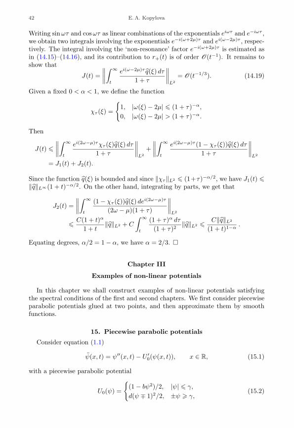
42 E.A. Kopylova
Writing sinωτ and cosωτ as linear combinations of the exponentials eiωτ and e−iωτ ,we obtain two integrals involving the exponentials e−i(ω+2µ)τ and ei(ω−2µ)τ , respec-tively. The integral involving the ‘non-resonance’ factor e−i(ω+2µ)τ is estimated asin (14.15)–(14.16), and its contribution to r+(t) is of order O(t−1). It remains toshow that
J(t) =∥∥∥∥∫ ∞
t
ei(ω−2µ)τ q(ξ) dτ1 + τ
∥∥∥∥L2
= O(t−1/3). (14.19)
Given a fixed 0 < α < 1, we define the function
χτ (ξ) =
1, |ω(ξ)− 2µ| 6 (1 + τ)−α,
0, |ω(ξ)− 2µ| > (1 + τ)−α.
Then
J(t) 6
∥∥∥∥∫ ∞
t
ei(2ω−µ)τχτ (ξ)q(ξ) dτ1 + τ
∥∥∥∥L2
+∥∥∥∥∫ ∞
t
ei(2ω−µ)τ (1− χτ (ξ))q(ξ) dτ1 + τ
∥∥∥∥L2
= J1(t) + J2(t).
Since the function q(ξ) is bounded and since ‖χτ‖L2 6 (1+τ)−α/2, we have J1(t) 6‖q‖L∞(1 + t)−α/2. On the other hand, integrating by parts, we get that
J2(t) =∥∥∥∥∫ ∞
t
(1− χτ (ξ))q(ξ) dei(2ω−µ)τ
(2ω − µ)(1 + τ)
∥∥∥∥L2
6C(1 + t)α
1 + t‖q‖L2 + C
∫ ∞
t
(1 + τ)α dτ
(1 + τ)2‖q‖L2 6
C‖q‖L2
(1 + t)1−α.
Equating degrees, α/2 = 1− α, we have α = 2/3.
Chapter III
Examples of non-linear potentials
In this chapter we shall construct examples of non-linear potentials satisfyingthe spectral conditions of the first and second chapters. We first consider piecewiseparabolic potentials glued at two points, and then approximate them by smoothfunctions.
15. Piecewise parabolic potentials
Consider equation (1.1)
ψ(x, t) = ψ′′(x, t)− U ′0(ψ(x, t)), x ∈ R, (15.1)
with a piecewise parabolic potential
U0(ψ) =
(1− bψ2)/2, |ψ| 6 γ,
d(ψ ∓ 1)2/2, ±ψ > γ,(15.2)

Asymptotic stability of solitons 43
where b, d > 0 and 0 < γ < 1 are constants. We want to determine conditions on band d under which U0(ψ) ∈ C1(R). Equating the values of the function U0 and itsderivative at γ gives
b =1γ, d =
11− γ
, 0 < γ < 1. (15.3)
We note that the second derivative U ′′0 (ψ) is a piecewise constant function withdiscontinuities at the points ψ = ±γ. Consider the stationary equation
s′′0(x) = U ′0(s0(x)) =
−bs0(x), 0 < s0(x) 6 γ,
d(s0(x)− 1), s0(x) > γ.(15.4)
We find a non-zero odd solution (kink) of this equation:
s0(x) =
C sin
√b x, 0 < x 6 q,
Ae−√
d x + 1, x > q,(15.5)
where C > γ, A < 0, and q = (1/√b ) arcsin(γ/C). Equating the values of the
function s0(x) and its derivative at x = q and using (15.3) for b and d, we see that
C =√γ , A = (γ − 1)e
√γ/(1−γ) arcsin
√γ , q =
√γ arcsin
√γ . (15.6)
15.1. The linearized equation. We linearize equation (15.1) near the kink s0(x)by representing the solution ψ(t) of this equation as the sum ψ(t) = s0 + φ(t).Substituting this into (15.1), we get that
φ(x, t) = φ′′(x, t)− U ′0(s0(x) + φ(x, t)) + U ′0(s0(x)).
Taking into account (15.2), we write the last equation as
φ(t) = −H0φ(t) + N (φ(t)), t ∈ R,
where
H0 = − d2
dx2+W0(x), W0(x) = U ′′0 (s0(x)) =
−b, |x| 6 q,
d, |x| > q.(15.7)
The continuous spectrum of the operator H0 coincides with [d,∞), and the discretespectrum lies in the interval [0, d]. The eigenfunction ϕ(x) corresponding to theeigenvalue λ satisfies the equation
−ϕ′′(x)− bϕ(x) = λϕ(x), |x| 6 q,
−ϕ′′(x) + dϕ(x) = λϕ(x), |x| > q.(15.8)
The eigenvalue λ0 = 0 is the ground state, and the positive even function ϕ0(x) =s′0(x) is the corresponding eigenfunction. Hence, the eigenfunction ϕ1(x) corre-sponding to the next eigenvalue λ1 > 0 (if it exists) must be odd.

44 E.A. Kopylova
15.2. Odd eigenfunctions. From equation (15.8) it is seen that the odd eigen-functions have the form
ϕ(x) =
B sinβx, |x| 6 q,
A(sgnx)e−α|x|, |x| > q,(15.9)
where α =√d− λ > 0 and β =
√b+ λ > 0. Equating the values of the function
ϕ(x) and its left and right derivatives at the point x = q, we have
Ae−αq = B sinβq, −Aαe−αq = Bβ cosβq, (15.10)
whereα2 + β2 = b+ d. (15.11)
The system (15.10) has a non-zero solution only if its determinant is zero, that is,
− α = β cotβq. (15.12)
We multiply both sides of equation (15.12) by q and let ξ = βq, η = αq. Takinginto account (15.11), we obtain the system of equations
− η = ξ cot ξ, ξ2 + η2 = R2, (15.13)
where R = q√b+ d denotes the radius of the circle on the (ξ, η)-plane. Substituting
the expressions for b, d, and q in terms of the parameter γ from (15.3) and (15.6),we see that
R =q√
γ(1− γ)=
arcsin√γ
√1− γ
. (15.14)
The solution of the system (15.13) can be found graphically (see Fig. 5). Consid-ering that η > 0, we get the following result:
R ∈ (0, π/2] : the system (15.13) has no solutions,R ∈ (π/2, 3π/2] : the system (15.13) has a unique solution,R ∈ (3π/2, 5π/2] : the system (15.13) has two solutions,. . . . . . . . . . . . . . . . . . . . . . . . . . . . . . . . . . . . . . . . . . . . . . . . . . . . . . . . . . . . .
(15.15)
Let γk, k ∈ N, denote the solution of the equation
arcsin√γk√
1− γk=kπ
2, k ∈ N. (15.16)
Solving this equation numerically, we find that
γ1 ∼ 0.64643, γ2 ∼ 0.8579, γ3 ∼ 0.92472, γ4 ∼ 0.95359, γ5 ∼ 0.96856, . . . .(15.17)
By (15.15),
γ ∈ (0, γ1] : there are no non-zero odd eigenfunctions,γ ∈ (γ1, γ3] : there exists one linearly independent odd
eigenfunction,γ ∈ (γ3, γ5] : there are two linearly independent odd
eigenfunctions,. . . . . . . . . . . . . . . . . . . . . . . . . . . . . . . . . . . . . . . . . . . . . . . . . . . . . . . .

Asymptotic stability of solitons 45
Figure 5. Graphical solution of the system (15.13)
In particular, for γ ∈ (γ1, γ3] we have one odd eigenfunction with the correspondingeigenvalue
λ1 = λ1(γ) = β2 − b =ξ2
q2− b =
1γ
(ξ2
arcsin2√γ− 1
)=
1γ
(sin2 ξ
1− γ− 1
), (15.18)
where ξ is the solution of the equation
ξ2
sin2 ξ=
arcsin2√γ1− γ
. (15.19)
15.3. Even eigenfunctions. From equation (15.8) it follows that even eigenfunc-tions have the form
ϕ(x) =
B cosβx, |x| 6 q,
Ae−α|x|, |x| > q.(15.20)
Proceeding as in the case of (15.13), we obtain the following equations for theparameters ξ = βq and η = αq:
η = ξ tan ξ, ξ2 + η2 = R2. (15.21)
The solution of this system can also be found graphically (see Fig. 6). The resultis:
R ∈ (0, π] : the system (15.21) has one solution,R ∈ (π, 2π] : the system (15.21) has two solutions,. . . . . . . . . . . . . . . . . . . . . . . . . . . . . . . . . . . . . . . . . . . . . . . . . . .
(15.22)
We note that, for any γ ∈ (0, 1), the function ξ = arcsin√γ ∈ (0, π/2) is a solution
of equation (15.21). This solution corresponds to the eigenvalue λ = 0 and the first
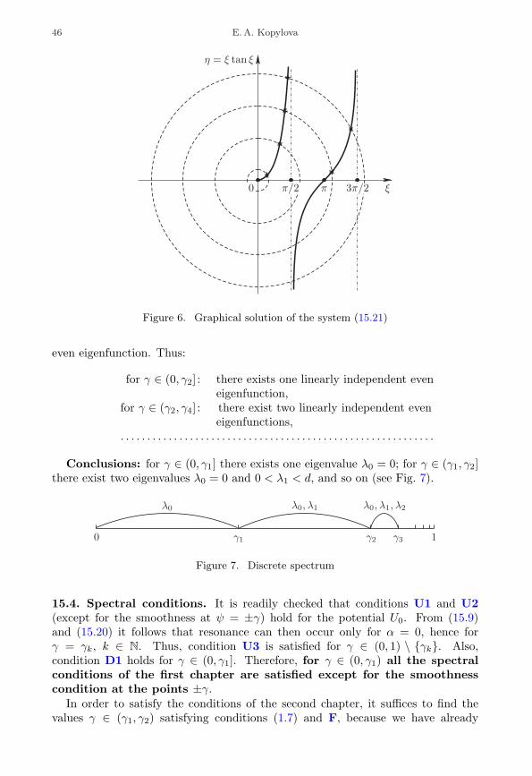
46 E.A. Kopylova
Figure 6. Graphical solution of the system (15.21)
even eigenfunction. Thus:
for γ ∈ (0, γ2] : there exists one linearly independent eveneigenfunction,
for γ ∈ (γ2, γ4] : there exist two linearly independent eveneigenfunctions,
. . . . . . . . . . . . . . . . . . . . . . . . . . . . . . . . . . . . . . . . . . . . . . . . . . . . . . . . . . .
Conclusions: for γ ∈ (0, γ1] there exists one eigenvalue λ0 = 0; for γ ∈ (γ1, γ2]there exist two eigenvalues λ0 = 0 and 0 < λ1 < d, and so on (see Fig. 7).
Figure 7. Discrete spectrum
15.4. Spectral conditions. It is readily checked that conditions U1 and U2(except for the smoothness at ψ = ±γ) hold for the potential U0. From (15.9)and (15.20) it follows that resonance can then occur only for α = 0, hence forγ = γk, k ∈ N. Thus, condition U3 is satisfied for γ ∈ (0, 1) \ γk. Also,condition D1 holds for γ ∈ (0, γ1]. Therefore, for γ ∈ (0, γ1) all the spectralconditions of the first chapter are satisfied except for the smoothnesscondition at the points ±γ.
In order to satisfy the conditions of the second chapter, it suffices to find thevalues γ ∈ (γ1, γ2) satisfying conditions (1.7) and F, because we have already

Asymptotic stability of solitons 47
proved that the operator H0 has exactly two eigenvalues (λ0 = 0 and λ1 ∈ (0, d))for these γ.
Lemma 15.1. Condition (1.7) holds for all γ ∈ (γ1, γ2). Condition F holds for allγ ∈ (γ1, γ2) except for a unique point γ∗.
Proof. 1) In view of (15.18) and (15.19) the inequality (1.7) with m2 = d is equiv-alent to the inequality
4γ
(sin2 ξ(γ)
1− γ− 1
)>
11− γ
,
where ξ(γ) ∈ (π/2, π) is the solution of equation (15.19). After some simple trans-formations, we get that 4 cos2 ξ(γ) < 3γ. Hence, it suffices to verify that
π
2< ξ(γ) < π − arccos
√3γ2
(15.23)
for all γ ∈ (γ1, γ2). The function ξ/ sin ξ is monotonically increasing on the interval(π/2, π), and thus the inequalities (15.23) are equivalent to
π
2<
arcsin√γ
√1− γ
<2(π − arccos(
√3γ/2))√
4− 3γ.
As a result, it follows that (1.7) is satisfied for γ1 < γ < α, where α is the solutionof the equation
arcsin√α√
1− α=
2(π − arccos(√
3α/2))√4− 3α
.
Approximate calculations show that α ∼ 0.921485 > γ2, and hence the inequal-ity (1.7) holds for all γ ∈ (γ1, γ2).
2) We write condition F as∫U ′′′0 (s0(x))ϕ4λ1(x)ϕ
2λ1
(x) dx =∫
d
dxU ′′0 (s0(x))
ϕ4λ1(x)ϕ2λ1
(x)s′0(x)
dx 6= 0. (15.24)
By (15.7)d
dxU ′′0 (s0(x)) = (b+ d)δ(x− q)− (b+ d)δ(x+ q),
so (15.24) means that ϕ4λ1(q)ϕ2λ1
(q) 6= 0. From formula (15.9) it follows thatϕλ1(q) = Ae−αq 6= 0. We show that the equality ϕ4λ1(q) = 0 holds for only onevalue γ ∈ (γ1, γ2). The function ϕ4λ1 is an odd solution of the equation
−ϕ′′4λ1(x)− bϕ4λ1(x) = 4λ1ϕ4λ1(x), |x| 6 q,
−ϕ′′4λ1(x) + dϕ4λ1(x) = 4λ1ϕ4λ1(x), |x| > q.
Hence, ϕ4λ1(q) = sinβq, where β =√b+ 4λ1 > 0. As a result, the equality
ϕ4λ1(q) = 0 is satisfied only if βq = kπ, k ∈ N, which is equivalent to the condition√1 + 4γλ1(γ) arcsin
√γ = kπ, k ∈ N.

48 E.A. Kopylova
Substituting here the expression for λ1(γ) from (15.18)–(15.19), we see that
arcsin√γ
√1− γ
√4 sin2 ξ − 3(1− γ) = kπ,
ξ2
sin2 ξ=
arcsin2√γ1− γ
. (15.25)
Since
0 <arcsin
√γ
√1− γ
√4 sin2 ξ − 3(1− γ) < 2π for γ ∈ (γ1, γ2),
it follows that k = 1. Let θ = arcsin√γ. Then the system (15.25) is equivalent to
the system
4ξ2 − 3θ2 = π2,sin ξξ
=cos θθ
. (15.26)
We find the solution graphically. Let us express θ in terms of ξ from the first andsecond equation and consider the corresponding functions θ1(ξ) and θ2(ξ). Thefunction θ1(ξ) :=
√(4ξ2 − π2)/3 is increasing on the interval (ξ(γ1), ξ(γ2)). In
addition,
θ′1(ξ) =1√3
4ξ√4ξ2 − π2
>1√3
4(π/2)√4(3π/4)2 − π2
=4√15
> 1, ξ(γ1) < ξ < ξ(γ2),
(15.27)because ξ(γ1) = π/2 and ξ(γ2) ∼ 2.3137 < 3π/4. The second function θ2(ξ) isimplicitly given by the equation (sin ξ)/ξ = (cos θ)/θ. Its derivative is
θ′2(ξ) =sin ξ − ξ cos ξ
ξ2θ2
cos θ + θ sin θ> 0,
π
2< ξ < ξ(γ2). (15.28)
Moreover, from (15.26),
θ′2(ξ) =θ
ξ
(sin ξ)/ξ − cos ξ(cos θ)/θ + sin θ
<(sin ξ)/ξ − cos ξ(sin ξ)/ξ + sin θ
< 1,π
2< ξ < ξ(γ2), (15.29)
since | cos ξ| < | cos ξ(γ2)| <√
2/2 and sin θ =√γ >
√γ
1>√
2/2 by (15.17).Furthermore,
θ2
(π
2
)> θ1
(π
2
)= 0, θ2(ξ(γ2)) ∼ 1.1843 < θ1(ξ(γ2)) ∼ 1.9616. (15.30)
From (15.27)–(15.30) it follows that θ1(ξ) = θ2(ξ) for only one value ξ(γ∗) ∈(π/2, ξ(γ2)) (see Fig. 8). Solving the system (15.26) numerically, we get γ∗ ∼ 0.7925.Thus, condition F holds for all γ ∈ (γ1, γ2) except for the one point γ∗.
Thus: for γ ∈ (γ1, γ∗) ∪ (γ∗, γ2) all the conditions of the second chapterare satisfied except for the smoothness condition for the potential at thepoints ±γ.
16. Smooth approximations
Let us approximate the potential U0 by smooth potentials. We consider an evenfunction h(ψ) ∈ C∞0 (R) such that h(ψ) > 0, supph ⊂ [−1, 1], and
∫h(ψ) dψ = 1.
Given any ε ∈ (0, γ), we set
Uε(ψ) :=1ε
∫h
(ψ − ψ′
ε
)U0(ψ′) dψ′. (16.1)
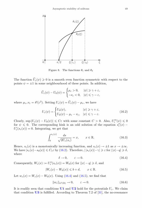
Asymptotic stability of solitons 49
Figure 8. The functions θ1 and θ2
The function Uε(ψ) > 0 is a smooth even function symmetric with respect to thepoints ψ = ±1 in some neighbourhood of these points. In addition,
Uε(ψ)− U0(ψ) =
µε > 0, |ψ| > γ + ε,
−νε < 0, |ψ| 6 γ − ε,
where µε, νε = O(ε2). Setting Uε(ψ) = Uε(ψ)− µε, we have
Uε(ψ) =
U0(ψ), |ψ| > γ + ε,
U0(ψ)− µε − νε, |ψ| 6 γ − ε.(16.2)
Clearly, sup |Uε(ψ) − U0(ψ)| 6 Cε with some constant C > 0. Also, U ′′′ε (ψ) 6 0for ψ 6 0. The corresponding kink is an odd solution of the equation s′′ε (x) −U ′ε(sε(x)) = 0. Integrating, we get that∫ sε(x)
0
ds√2Uε(sε)
= x, x ∈ R. (16.3)
Hence, sε(x) is a monotonically increasing function, and sε(x) → ±1 as x→ ±∞.We have |sε(x)−s0(x)| 6 C1ε by (16.2). Therefore, | |sε(x)|−γ| > ε for | |x|−q| > δ,where
δ → 0, ε→ 0. (16.4)
Consequently, Wε(x) := U ′′ε (sε(x)) = W0(x) for ||x| − q| > δ, and
|Wε(x)−W0(x)| 6 b+ d, x ∈ R. (16.5)
Let wε(x) = Wε(x)−W0(x). Using (16.4) and (16.5), we find that
‖wε‖L2(R) → 0, ε→ 0. (16.6)
It is readily seen that conditions U1 and U2 hold for the potentials Uε. We claimthat condition U3 is fulfilled. According to Theorem 7.2 of [31], the no-resonance

50 E.A. Kopylova
condition at an edge point of the continuous spectrum is equivalent to the require-ment that the resolvent be bounded at this point. The resolvents R0(ω) and Rε(ω)of the operators H0 and Hε := −d2/dx2 +Wε(x) are related by the equation
Rε(ω) = R0(ω)(1 + wεR0(ω))−1, (16.7)
from which it follows by (16.6) that the potentials Uε(ψ) satisfy condition U3 forsufficiently small ε > 0 and all γ ∈ (0, 1) \ γk.
From (16.6) and (16.7) it also follows that the eigenvalues of the operator Hε
converge to eigenvalues of the operator H0 as ε→ 0. As a result:i) for all γ ∈ (0, γ1) and sufficiently small ε, the operator Hε has only the one
eigenvalue zero, that is, the potentials Uε satisfy the spectral condition D1;ii) for γ ∈ (γ1, γ2) and sufficiently small ε, the operator Hε has two eigenvalues
λ0 = 0 and 0 < λ1(ε) < d, with 4λ1(ε) > d, that is, the potentials Uε satisfy thespectral condition D2.
It is easily checked that condition F is also satisfied for small ε and all γ ∈(γ1, γ2) \ γ∗.
Bibliography
[1] S. Agmon, “Spectral properties of Schrodinger operators and scattering theory”,Ann. Scuola Norm. Sup. Pisa Cl. Sci. (4) 2:2 (1975), 151–218.
[2] N. Boussaid, “Stable directions for small nonlinear Dirac standing waves”, Comm.Math. Phys. 268:3 (2006), 757–817.
[3] N. Boussaid and S. Cuccagna, “On stability of standing waves of nonlinear Diracequations”, Comm. Partial Differential Equations 37:6 (2012), 1001–1056; arXiv:1103.4452v3.
[4] V. S. Buslaev, A. I. Komech, E.A. Kopylova, and D. Stuart, “On asymptoticstability of solitary waves in Schrodinger equation coupled to nonlinear oscillator”,Comm. Partial Differential Equations 33:4-6 (2008), 669–705.
[5] В. С. Буслаев, Г. С. Перельман, “Рассеяние лля нелинейного уравненияШрёдингера: состояния, близкие к солитону”, Алгебра и анализ 4:6 (1992),63–102; English transl., V. S. Buslaev and G. S. Perelman, “Scattering for thenonlinear Schrodinger equation: states close to a soliton”, St. Petersburg Math. J.4:6 (1993), 1111–1142.
[6] V. S. Buslaev and G. S. Perelman, “On the stability of solitary waves for nonlinearSchrodinger equations”, Nonlinear evolution equations, Amer. Math. Soc. Transl.Ser. 2, vol. 164, Amer. Math. Soc., Providence, RI 1995, pp. 75–98.
[7] V. S. Buslaev and C. Sulem, “On asymptotic stability of solitary waves fornonlinear Schrodinger equations”, Ann. Inst. H. Poincare Anal. Non Lineaire 20:3(2003), 419–475.
[8] S. Cuccagna, “Stabilization of solutions to nonlinear Schrodinger equations”,Comm. Pure Appl. Math. 54:9 (2001), 1110–1145.
[9] S. Cuccagna, “On asymptotic stability in 3D of kinks for the φ4 model”, Trans.Amer. Math. Soc. 360:5 (2008), 2581–2614.
[10] W. Eckhaus and A. van Harten, The inverse scattering transformation andthe theory of solitons. An introduction, North-Holland Math. Stud., vol. 50,North-Holland Publishing Co., Amsterdam–New York 1981, xi+222 pp.
[11] A. S. Fokas and V.E. Zakharov (eds.), Important developments in soliton theory,Springer Ser. Nonlinear Dynam., Springer-Verlag, Berlin 1993, x+559 pp.

Asymptotic stability of solitons 51
[12] C. S. Gardner, J.M. Greene, M. D. Kruskal, and R. M. Miura, “Method for solvingthe Korteweg–de Vries equation”, Phys. Rev. Lett. 19 (1967), 1095–1097.
[13] W. Heisenberg, “Der derzeitige Stand der nichtlinearen Spinortheorie derElementarteilchen”, Acta Phys. Austriaca 14 (1961), 328–339.
[14] W. Heisenberg, Introduction to the unified field theory of elementary particles,Interscience Publishers, London–New York–Sydney 1966, ix+177 pp.
[15] V. Imaykin, A. Komech, and H. Spohn, “Scattering asymptotics for a chargedparticle coupled to the Maxwell field”, J. Math. Phys. 52:4 (2011), 042701, 33 pp.
[16] V. Imaikin, A. Komech, and B. Vainberg, “On scattering of solitons for theKlein–Gordon equation coupled to a particle”, Comm. Math. Phys. 268:2 (2006),321–367.
[17] E. Kirr and A. Zarnesku, “On the asymptotic stability of bound states in 2D cubicSchrodinger equation”, Comm. Math. Phys. 272:2 (2007), 443–468.
[18] A. Komech and E. Kopylova, “Scattering of solitons for Schrodinger equationcoupled to a particle”, Russ. J. Math. Phys. 13:2 (2006), 158–187; arXiv:math/0609649.
[19] A. I. Komech and E. A. Kopylova, “Weighted energy decay for 1D Klein–Gordonequation”, Comm. Partial Differential Equations 35:2 (2010), 353–374.
[20] A. I. Komech, E. A. Kopylova, and H. Spohn, “Scattering of solitons for Diracequation coupled to a particle”, J. Math. Anal. Appl. 383:2 (2011), 265–290;arXiv: 1012.3109.
[21] A. Komech, E. Kopylova, and D. Stuart, “On asymptotic stability of solitonsin a nonlinear Schrodinger equation”, Commun. Pure Appl. Anal. 11:3 (2012),1063–1079; arXiv: 0807.1878.
[22] A. I. Komech, N. J. Mauser, and A.P. Vinnichenko, “Attraction to solitons inrelativistic nonlinear wave equations”, Russ. J. Math. Phys. 11:3 (2004), 289–307.
[23] E. Kopylova, “On the asymptotic stability of solitary waves in the discreteSchrodinger equation coupled to a nonlinear oscillator”, Nonlinear Anal. 71:7-8(2009), 3031–3046; arXiv: 0805.3403.
[24] Е. А. Копылова, “Дисперсионные оценки для уравнений Шрёдингераи Клейна–Гордона”, УМН 65:1(391) (2010), 97–144; English transl.,E. A. Kopylova, “Dispersive estimates for the Schrodinger and Klein–Gordonequation”, Russian Math. Surveys 65:1 (2010), 95–142.
[25] E. A. Kopylova, “On asymptotic stability of solitary waves in discrete Klein–Gordonequation coupled to nonlinear oscillator”, Appl. Anal. 89:9 (2010), 1467–1492.
[26] E. Kopylova, “On long-time decay for modified Klein–Gordon equation”, Commun.Math. Anal. Conference 03 (2011), 137–152; arXiv: 1009.2649.
[27] E. A. Kopylova and A. I. Komech, “On asymptotic stability of moving kink forrelativistic Ginzburg–Landau equation”, Comm. Math. Phys. 302:1 (2011),225–252; arXiv: 0910.5538.
[28] E. Kopylova and A. I. Komech, “On asymptotic stability of kink for relativisticGinzburg–Landau equation”, Arch. Ration. Mech. Anal. 202:1 (2011), 213–245;arXiv: 0910.5539.
[29] J.-L. Lions, Quelques methodes de resolution des problemes aux limites nonlineaires, Dunod, Paris; Gauthier-Villars, Paris 1969, xx+554 pp.
[30] J. R. Miller and M. I. Weinstein, “Asymptotic stability of solitary waves for theregularized long-wave equation”, Comm. Pure Appl. Math. 49:4 (1996), 399–441.
[31] M. Murata, “Asymptotic expansions in time for solutions of Schrodinger-typeequations”, J. Funct. Anal. 49:1 (1982), 10–56.

52 E.A. Kopylova
[32] R. L. Pego and M. I. Weinstein, “Asymptotic stability of solitary waves”, Comm.Math. Phys. 164:2 (1994), 305–349.
[33] D. E. Pelinovsky and A. A. Stefanov, “Asymptotic stability of small gap solitonsin nonlinear Dirac equations”, J. Math. Phys. 53:7 (2012), 073705, 27 pp.; arXiv:1008.4514.
[34] C.-A. Pillet and C.E. Wayne, “Invariant manifolds for a class of dispersive,Hamiltonian, partial differential equations”, J. Differential Equations 141:2 (1997),310–326.
[35] M. Reed, Abstract non-linear wave equations, Lecture Notes in Math., vol. 507,Springer-Verlag, Berlin–New York 1976, vi+128 pp.
[36] M. Reed and B. Simon, Methods of modern mathematical physics, vol. III:Scattering theory, Academic Press, New York–London 1979, xv+463 pp.
[37] I. Rodnianski, W. Schlag, and A. Soffer, “Dispersive analysis of charge transfermodels”, Comm. Pure Appl. Math. 58:2 (2005), 149–216.
[38] A. Soffer and M. I. Weinstein, “Multichannel nonlinear scattering for nonintegrableequations”, Comm. Math. Phys. 133:1 (1990), 119–146.
[39] A. Soffer and M. I. Weinstein, “Multichannel nonlinear scattering for nonintegrableequations. II. The case of anisotropic potentials and data”, J. Differential Equations98:2 (1992), 376–390.
[40] A. Soffer and M. I. Weinstein, “Resonances, radiation damping and instability inHamiltonian nonlinear wave equations”, Invent. Math. 136:1 (1999), 9–74.
[41] W. A. Strauss, “Nonlinear invariant wave equations”, Invariant wave equations,Proceedings of the “Ettore Majorana” International School of Mathematical Physics(Erice, 1977), Lecture Notes in Phys., vol. 73, Springer, Berlin–New York 1978,pp. 197–249.
[42] Tai-Peng Tsai and Horng-Tzer Yau, “Asymptotic dynamics of nonlinearSchrodinger equations: resonance-dominated and dispersion-dominated solutions”,Comm. Pure Appl. Math. 55:2 (2002), 153–216.
[43] Tai-Peng Tsai, “Asymptotic dynamics of nonlinear Schrodinger equations withmany bound states”, J. Differential Equations 192:1 (2003), 225–282.
[44] M. Weinstein, “Modulational stability of ground states of nonlinear Schrodingerequations”, SIAM J. Math. Anal. 16:3 (1985), 472–491.
[45] N. J. Zabusky and M. D. Kruskal, “Interaction of ‘solitons’ in a collisionless plasmaand the recurrence of initial states”, Phys. Rev. Lett. 15 (1965), 240–243.
E.A. KopylovaKharkevich Institute for Information TransmissionProblems, Russian Academy of Sciences;University of Vienna, AustriaE-mail : [email protected]
Received 6/FEB/13Translated by A. ALIMOV