Asymptotic preserving schemes (AP)for magnetically confined ...
42
C. Negulescu, 15/10/2013 1 Asymptotic preserving schemes (AP) for magnetically confined plasmas Highly anisotropic elliptic/parabolic equations Claudia Negulescu Institut de Mathématiques de Toulouse Université Paul Sabatier
Transcript of Asymptotic preserving schemes (AP)for magnetically confined ...

C. Negulescu, 15/10/2013
1
Asymptotic preserving schemes (AP) formagnetically confined plasmas
Highly anisotropic elliptic/parabolic equations
Claudia Negulescu
Institut de Mathématiques de Toulouse
Université Paul Sabatier

C. Negulescu, 15/10/2013
2Introduction/Motivation
Objective: Numerical study of highly anisotropic, multi-scale problems
• Many pb. in nature exhibit multi-scale behaviours, which can be
rather different in character
• Typical: occurence of one or several small/large parameters
(Reynolds, Peclet, Mach nbr. etc)
• General, unified treatment is impossible
C. Negulescu, 15/10/2013
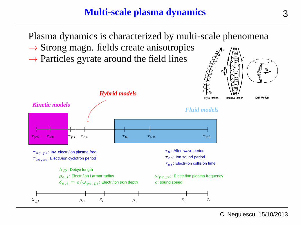
3Multi-scale plasma dynamics
Plasma dynamics is characterized by multi-scale phenomena→ Strong magn. fields create anisotropies→ Particles gyrate around the field lines
Kinetic modelsFluid models
Hybrid models
τpe τce τpi τci τa τcs τei
Lρe ρi
τa : Alfen wave period
τcs : Ion sound period
τei : Electr-ion collision time
τpe,pi : Inv. electr./ion plasma freq.
τce,ci : Electr./ion cyclotron period
λD : Debye length
ρe,i : Electr./ion Larmor radius
c: sound speed
δe δi
δe,i = c/ωpe,pi : Electr./ion skin depth
ωpe,pi : Electr./ion plasma frequency
λD

C. Negulescu, 15/10/2013
4Multi-scale problems
A small-scale numerical simulation is out of reach
requires mesh-sizes dependent on small scale param.ε≪ 1
excessive computational time and memory space are needed tocapture small scales
It is not always of interest to resolve the details at the smallscale. Multi-scale strategies are much more adequate!
homogeneisation, domain decomposition, multi-grids, multi-scalemethods based on wavelets or finite elements, multi-scalevariational methods
Essential feature of these methods
capture efficiently the large scale behavior of the solution, withoutresolving the small scale features

C. Negulescu, 15/10/2013
5Asymptotic Preserving schemes
Difficulty: Resolution of multiscale pb. can be very difficult, ifthe pb. becomes singular, as one of the parametersε→ 0
(P ε) sing. perturbed pb. with sol.fε
the seq.fε converges towardsf0, sol. of a limit pb.(P 0)
the limit pb. (P 0) is different in type from the initial(P ε)
standard schemes would require∆t,∆x ∼ ε for stability
Definition: A schemeP ε,h is AP iff it is convergent forh→ 0uniformely inε, i.e.
P ε,h P ε
P 0,h P 0
ε→
0
ε→
0
h→ 0
h→ 0

C. Negulescu, 15/10/2013
6Asymptotic Preserving schemes
AP-procedure:
requires that the limit problem(P 0) is identified andwell-posed
consists in trying to mimic at discrete level the asymptoticbehaviour of the sing. perturbed pb. sol.fε
requires a sufficient degree of implicitness (not obvious)
Advantages:
gives accurate and stable results, with no restrictions onthe computational mesh
enables to capture automatically the Limit modelP 0, ifε→ 0 (micro-macro transition)
no more coupling needed, ifε(x) is variable

C. Negulescu, 15/10/2013
7Kinetic models and specific limit regimes
• Fundamental kinetic model: Vlasov/Boltzmann equation
∂tf + v · ∇xf +q
m(E + v ×B) · ∇vf = Q(f)
Several small scales/parameters occur, leading to diff. regimes:• Hydrodynamic scaling[Filbet/Jin; Dimarco/Pareschi]
∂tf + v · ∇xf =1
εQ(f)
0 < ε≪ 1: mean free path (Knudsen nbr.)
in the limit ε→ 0, one gets the compressible Euler eq.
AP-scheme: Decomposition of the source term in stiff-and non-stiff part
Q(f)
ε=Q(f)− P (f)
ε+P (f)
ε
C. Negulescu, 15/10/2013
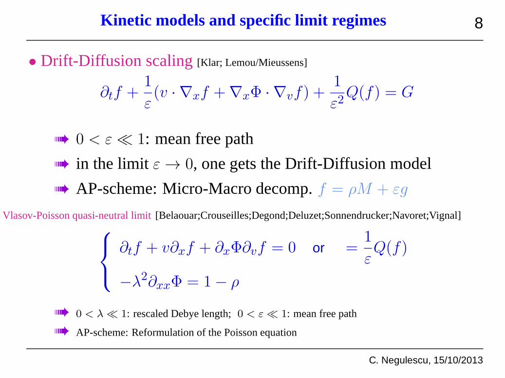
8Kinetic models and specific limit regimes
• Drift-Diffusion scaling[Klar; Lemou/Mieussens]
∂tf +1
ε(v · ∇xf +∇xΦ · ∇vf) +
1
ε2Q(f) = G
0 < ε≪ 1: mean free path
in the limit ε→ 0, one gets the Drift-Diffusion model
AP-scheme: Micro-Macro decomp.f = ρM + εg
• Vlasov-Poisson quasi-neutral limit[Belaouar;Crouseilles;Degond;Deluzet;Sonnendrucker;Navoret;Vignal]
∂tf + v∂xf + ∂xΦ∂vf = 0 or =1
εQ(f)
−λ2∂xxΦ = 1− ρ
0 < λ≪ 1: rescaled Debye length;0 < ε≪ 1: mean free path
AP-scheme: Reformulation of the Poisson equation
C. Negulescu, 15/10/2013
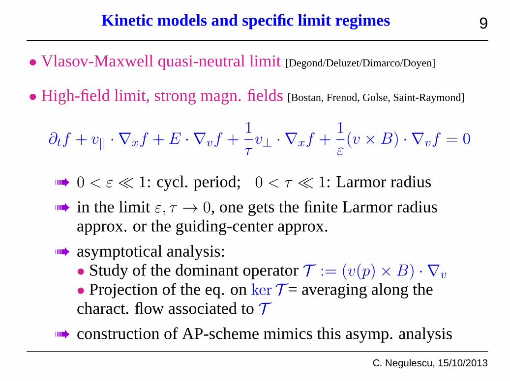
9Kinetic models and specific limit regimes
• Vlasov-Maxwell quasi-neutral limit[Degond/Deluzet/Dimarco/Doyen]
• High-field limit, strong magn. fields[Bostan, Frenod, Golse, Saint-Raymond]
∂tf + v|| · ∇xf + E · ∇vf +1
τv⊥ · ∇xf +
1
ε(v × B) · ∇vf = 0
0 < ε≪ 1: cycl. period; 0 < τ ≪ 1: Larmor radius
in the limit ε, τ → 0, one gets the finite Larmor radiusapprox. or the guiding-center approx.
asymptotical analysis:• Study of the dominant operatorT := (v(p)× B) · ∇v
• Projection of the eq. onker T = averaging along thecharact. flow associated toT
construction of AP-scheme mimics this asymp. analysis

C. Negulescu, 15/10/2013
10Fluid models and specific limit regimes
• Euler-Poisson quasi-neutral limit[Crispel/Degond/Vignal]
∂tn+∇ · (nu) = 0
∂t(nu) +∇ · (nu⊗ u) +∇p(n) = n∇Φ
−λ2∆Φ = 1− n
0 < λ≪ 1: rescaled Debye length
• High-field limit, Euler-Lorentz[Brull;Degond;Deluzet;Mouton;Sangam;Vignal]
∂tn+∇ · (nu) = 0
∂t(nu) +∇ · (nu⊗ u) +1
τ∇p(n) =
1
τn (E + u× B)
0 < τ ≪ 1: rescaled gyro-period

C. Negulescu, 15/10/2013
11Fluid models and specific limit regimes
• Low Mach-nbr. limit[Degond/Tang; Cordier/Degond/Kumbaro]
∂tn+∇ · (nu) = 0
∂t(nu) +∇ · (nu⊗ u) +1
ε2∇p(n) = 0
0 < ε≪ 1: rescaled Mach-nbr.
in the limit ε→ 0, one gets the incompressible Euler eq.
AP-scheme: Stiff term is decomposed as
1
ε2∇p(n) = α∇p(n) +
1− αε2
ε2∇p(n)
• Highly anisotropic potential/temp. eq.[Deluzet/Lozinski/Mentrelli/Narski/Negulescu]
−1
ε∇|| · (A||∇||φ)−∇⊥ · (A⊥∇⊥φ) = f
∂tT −1
ε∇|| · (K||∇||T )−∇⊥ · (K⊥∇⊥T ) = 0

C. Negulescu, 15/10/2013
12
Anisotropic elliptic equation
Work based on:
[1] P. Degond, F. Deluzet, C. Negulescu "An asymptotic preserving scheme for strongly
anisotropic elliptic problems", SIAM-MMS.
[2] P. Degond, F. Deluzet, A. Lozinski, J. Narski, C. Negulescu "Duality based
Asymptotic-Preserving Method for highly anisotropic diffusion equations", CMS.
[3] P. Degond, A. Lozinski, J. Narski, C. Negulescu "An Asymptotic-Preserving method for
highly anisotropic elliptic equations based on a micro-macro decomposition", JCP.

C. Negulescu, 15/10/2013
13Introduction/Motivation
Macroscopic nature of magnetically confined plasma dynamicscan be described via the one-fluid (MHD) model• Continuity equation of plasma charge
∂tρc + div · j = 0 ,
ρc := qni − ene , j = qniui − eneue , q = eZ
• Quasi-neutrality (|ne − Zni| ≪ ne) implies
ρc ≈ 0 ⇒ ∇ · j = 0
• Ohm’s law
j = σ(E + v × B) , v =nemeue + nimiuineme + nimi
, E = −∇φ

C. Negulescu, 15/10/2013
14Mathematical problem
Theme: Numerical resolution of highly anisotropic elliptic eq.
−∇ · (A∇φ) = f , on Ω
φ = 0 on ∂ΩD , ∂zφ = 0 on ∂Ωz ,
whereΩ ⊂ R2 or Ω ⊂ R3 and∂Ω = ∂ΩD ∪ ∂Ωz.• Diffusion matrixA is given by
A =
(
A⊥ 0
0 1
εAz
)
, −∂
∂x
(
A⊥∂φ
∂x
)
−1
ε
∂
∂z
(
Az∂φ
∂z
)
= f ,
• A⊥, Az of same order of magnitude, bounded from below/above• 0 < ε≪ 1 very small
• anisotropy aligned with thez-coordinate

C. Negulescu, 15/10/2013
15The Singular Perturbation pb. (P-model)
(P )
−∂
∂x
(
A⊥∂φ
∂x
)
−1
ε
∂
∂z
(
Az∂φ
∂z
)
= f , on Ω ,
∂φ
∂z= 0 on Ωx × ∂Ωz , φ = 0 on ∂Ωx × Ωz ,
Letting formallyε→ 0, yields the reduced problem (R-model)
(R)
−∂
∂z
(
Az∂φ
∂z
)
= 0 , on Ω ,
∂φ
∂z= 0 on Ωx × ∂Ωz , φ = 0 on ∂Ωx × Ωz ,
→ R is an ill-posed problem !
→ R exhibits an infinit amount of solutionsφ(x).

C. Negulescu, 15/10/2013
16The Limit problem (L-model)
• Numerical burden: Discretization matrix of P-model is very
ill-conditioned, cond ∼ 1ε .
→ standard resolution meth. for lin. syst. no more efficient for 0 < ε << 1
• However,φε (sol. of P-model)→ε→0 φ0, sol. of
(L)
−∂
∂x
(
A⊥∂φ
∂x
)
= f(x) , on Ωx ,
φ = 0 on ∂Ωx ,
wheref(x) := 1Lz
∫ Lz
0 f(x, z)dz is the average alongz-coord.
Identification of Limit-model:
Supposeφε → φ0, whereφ0(x) dep. only onx
Integrate(Pε) in z and pass to the limitε→ 0
Averaging inz is the proj. on the kernel of dominant op.

C. Negulescu, 15/10/2013
17Transition between(Pε) and (L) pb.
Let us denote by:
|| the direction of the anisotropy (herez-direction)
⊥ the perpendicular direction (herex-direction) the bilinear forms
a||(φ, ψ) :=
∫
ΩA||∇||φ · ∇||ψ dx dz , a⊥(φ, ψ) :=
∫
Ω(A⊥∇⊥φ) · ∇⊥ψ dx dz .
How to switch from sing. perturbed pb.: findφε ∈ V , sol. of
(Pε) a||(φε, ψ) + εa⊥(φ
ε, ψ) = ε(f, ψ) , ∀ψ ∈ V ,
to Limit model: findφ0 ∈ G, sol. of
(L) a⊥(φ0, ψ) = ε(f, ψ) , ∀ψ ∈ G ,
Goal: AP-scheme which switches automatically, with no hugh num. costs

C. Negulescu, 15/10/2013
18Duality-Based decomposition
• Introduction of mathematical framework
V := φ ∈ H1(Ω) / φ|∂ΩD= 0 , (φ, ψ)V := (∇||φ,∇||ψ)L2 + ε(∇⊥φ,∇⊥ψ)L2
• Identification of Kernel of dominant operator
G := φ ∈ V | ∇‖φ = 0 , (φ, ψ)G := (∇⊥φ,∇⊥ψ)L2 ,
A := φ ∈ V |(φ, ψ) = 0 , ∀ψ ∈ G = φ ∈ V |∫
Lzφ(x, z) dz = 0
• Definition of the orthogonal projection on the Kernel
P : V → G such thatPφ :=1
Lz
∫
Lz
φ(x, z) dz
• Definition of decompositionV = G ⊕⊥ A
φε ∈ V ⇒ φε = pε + qε , pε = Pφε ∈ G , qε = (I − P )φε ∈ A
C. Negulescu, 15/10/2013
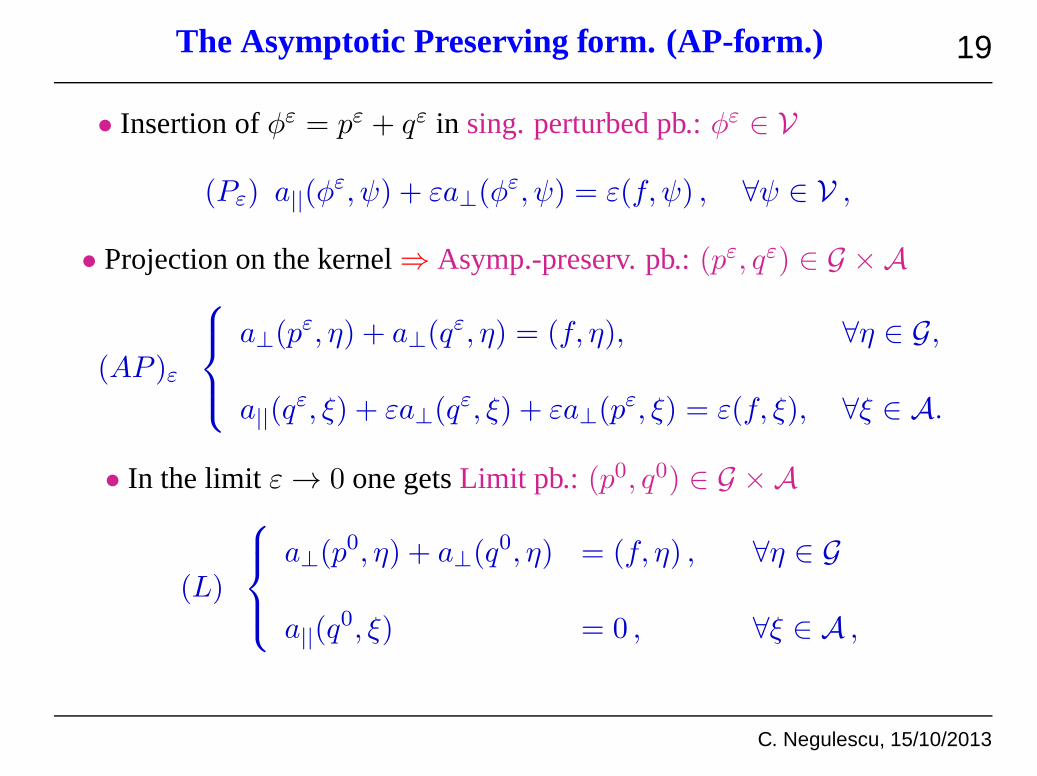
19The Asymptotic Preserving form. (AP-form.)
• Insertion ofφε = pε + qε in sing. perturbed pb.:φε ∈ V
(Pε) a||(φε, ψ) + εa⊥(φ
ε, ψ) = ε(f, ψ) , ∀ψ ∈ V ,
• Projection on the kernel⇒ Asymp.-preserv. pb.:(pε, qε) ∈ G × A
(AP )ε
a⊥(pε, η) + a⊥(q
ε, η) = (f, η), ∀η ∈ G,
a||(qε, ξ) + εa⊥(q
ε, ξ) + εa⊥(pε, ξ) = ε(f, ξ), ∀ξ ∈ A.
• In the limit ε→ 0 one getsLimit pb.: (p0, q0) ∈ G × A
(L)
a⊥(p0, η) + a⊥(q
0, η) = (f, η) , ∀η ∈ G
a||(q0, ξ) = 0 , ∀ξ ∈ A ,

C. Negulescu, 15/10/2013
20Summary of the AP-idea
P-model AP-model
R-model L-model
ǫ → 0 ǫ → 0
reform.
ǫ → 0
φǫ = φ′ǫ + φǫ
φǫ ∈ V
equiv.
reform.
(sol. of (P)) (sol. of (AP))
(sol. of (L))
(φ′ǫ, φǫ) ∈ A × G
(0, φ0) ∈ A × G
V := ψ(·, ·) ∈ H1(Ω) / ψ = 0 on ∂Ωx × Ωz V = G ⊕⊥ A
G := φ ∈ V | ∇‖φ = 0 = φ(·) ∈ H1(Ωx) / φ = 0 on ∂Ωx ,
A := φ ∈ V |(φ, ψ) = 0 , ∀ψ ∈ G = φ ∈ V |
∫
Lz
φ(x, z) dz = 0
C. Negulescu, 15/10/2013
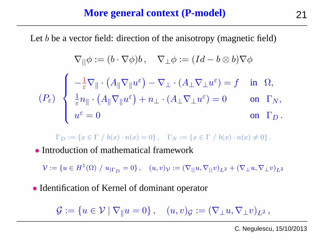
21More general context (P-model)
Let b be a vector field: direction of the anisotropy (magnetic field)
∇||φ := (b · ∇φ)b , ∇⊥φ := (Id− b⊗ b)∇φ
(Pε)
−1ε∇‖ ·
(
A‖∇‖uε)
−∇⊥ · (A⊥∇⊥uε) = f in Ω,
1εn‖ ·
(
A‖∇‖uε)
+ n⊥ · (A⊥∇⊥uε) = 0 on ΓN ,
uε = 0 on ΓD .
ΓD := x ∈ Γ / b(x) · n(x) = 0 , ΓN := x ∈ Γ / b(x) · n(x) 6= 0 .
• Introduction of mathematical framework
V := u ∈ H1(Ω) / u|ΓD= 0 , (u, v)V := (∇||u,∇||v)L2 + (∇⊥u,∇⊥v)L2
• Identification of Kernel of dominant operator
G := u ∈ V | ∇‖u = 0 , (u, v)G := (∇⊥u,∇⊥v)L2 ,

C. Negulescu, 15/10/2013
22Limit problem (L-model)
The solutionuε of pb. (P )ε
(P )ε
∫
ΩA||∇||u
ε · ∇||v dx+ ε
∫
Ω(A⊥∇⊥u
ε) · ∇⊥v dx = ε(f, v) , ∀v ∈ V ,
converges forε→ 0 towardsu0, sol. of
(L)
∫
Ω(A⊥∇⊥u
0) · ∇⊥v dx =
∫
Ωfv dx , ∀v ∈ G .
P-model AP-model
R-model L-model
ǫ → 0 ǫ → 0
reform.
ǫ → 0
equiv.
reform.
(sol. of (P)) (sol. of (AP))
(sol. of (L))
uǫ ∈ V (uǫ, qǫ) ∈ V × L
(u0, q0) ∈ V × L
∇||pǫ = 0
uǫ = pǫ + ǫqǫ
Goal: AP-scheme which switches automatically between(Pε) and(L).
C. Negulescu, 15/10/2013
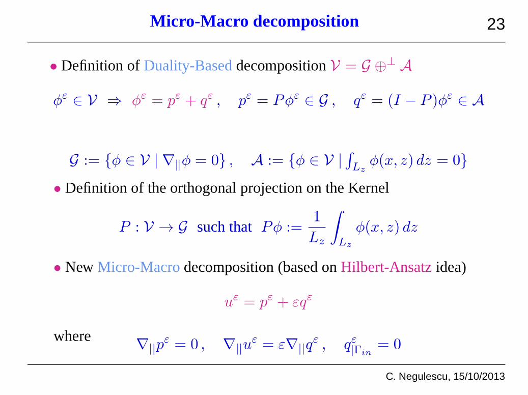
23Micro-Macro decomposition
• Definition of Duality-BaseddecompositionV = G ⊕⊥ A
φε ∈ V ⇒ φε = pε + qε , pε = Pφε ∈ G , qε = (I − P )φε ∈ A
G := φ ∈ V | ∇‖φ = 0 , A := φ ∈ V |∫
Lzφ(x, z) dz = 0
• Definition of the orthogonal projection on the Kernel
P : V → G such thatPφ :=1
Lz
∫
Lz
φ(x, z) dz
• NewMicro-Macrodecomposition (based onHilbert-Ansatzidea)
uε = pε + εqε
where∇||p
ε = 0 , ∇||uε = ε∇||q
ε , qε|Γin= 0
C. Negulescu, 15/10/2013
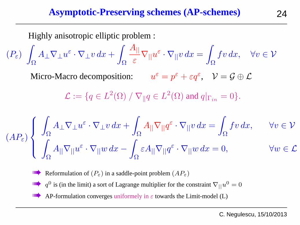
24Asymptotic-Preserving schemes (AP-schemes)
Highly anisotropic elliptic problem :
(Pε)
∫
ΩA⊥∇⊥u
ε · ∇⊥v dx+
∫
Ω
A||
ε∇||u
ε · ∇||v dx =
∫
Ωfv dx, ∀v ∈ V
Micro-Macro decomposition: uε = pε + εqε, V = G ⊕ L
L := q ∈ L2(Ω) /∇‖q ∈ L2(Ω) andq|Γin = 0.
(APε)
∫
ΩA⊥∇⊥u
ε · ∇⊥v dx+
∫
ΩA||∇||q
ε · ∇||v dx =
∫
Ωfv dx, ∀v ∈ V
∫
ΩA||∇||u
ε · ∇||w dx−
∫
ΩεA||∇||q
ε · ∇||w dx = 0, ∀w ∈ L
Reformulation of(Pε) in a saddle-point problem(APε)
q0 is (in the limit) a sort of Lagrange multiplier for the constraint∇||u0 = 0
AP-formulation convergesuniformely inε towards the Limit-model (L)

C. Negulescu, 15/10/2013
25Numerical results
• Exact solutionuεe, Num. sol. (AP)uεA, Num. sol. (P)uεP , Num.sol. (L)uεL
uεe = sin(
πy + α(y2 − y) cos(πx))
+ ε cos (2πx) sin (πy)
100
10000
1e+06
1e+08
1e+10
1e+12
1e+14
1e+16
1e+18
1e+20
1e-30 1e-25 1e-20 1e-15 1e-10 1e-05 1
(P)(MM)(DB)
→ Cond. of the discretization matrix of pb. (P) degenerates ifε→ 0, whereas it remainsε-independent for the AP-scheme

C. Negulescu, 15/10/2013
26Numerical results
1e-07
1e-06
1e-05
0.0001
0.001
0.01
0.1
1
10
1e-15 1e-10 1e-05 1
(P)(L)
(AP)
1e-05
0.0001
0.001
0.01
0.1
1
10
100
1e-15 1e-10 1e-05 1
(P)(L)
(AP)
The AP-scheme is unif. precise inε, of order3 in theL2-norm and of order2 in theH1-norm (Q2-FE)
This AP-scheme does not require to adapt the grid withrespect to the fieldb
The AP-formulation can treat variable anisotropies

C. Negulescu, 15/10/2013
27
Anisotropic parabolic equation
Work based on:
[1] A. Mentrelli, C. Negulescu "Asymptotic-Preserving schemefor highly anisotropic non-linear
diffusion equations", Journal of Comp. Phys.
[2] A. Lozinski, J. Narski, C. Negulescu "Highly anisotropic temperature balance equation and its
asymptotic-preserving resolution", submitted to M2AN.

C. Negulescu, 15/10/2013
28Introduction/Motivation
• Two-fluid description of plasma dynamics
∂tnα +∇ · (nαuα) = Snα ,
mαnα [∂tuα + (uα · ∇)uα] = nαeα(E + uα ×B)−∇ · Pα +Rα ,
32nαkB [∂tTα + (uα · ∇)Tα] = −∇ · qα − Pα : ∇uα +Qα ,
• Fourier law:qα := −κα∇Tα
• Anisotropy due to the magn. field:κα,|| ∼ T5/2α , κα,⊥ indep. onTα
Theme: Efficient numerical resolution of temperature equation
∂tT −1
ε∇|| · (K||T
5/2∇||T )−∇⊥ · (K⊥∇⊥T ) = 0,
whereT := T||T ||∞
andε := 1
||T ||5/2∞
≪ 1 → Anisotropic, degenerate
nonlinear parabolic equation

C. Negulescu, 15/10/2013
29The 2D temperature balance equation
(Pε)
∂tT − 1ε∇|| · (K||T
5/2∇||T )−∇⊥ · (K⊥∇⊥T ) = 0 , in [0, S]× Ω ,
1εn|| · (K||T
5/2(t, ·)∇||T (t, ·)) + n⊥ · (K⊥∇⊥T (t, ·)) = −γT (t, ·) , on [0, S]× Γ⊥ ,
∇⊥T (t, ·) = 0 , on [0, S]× Γ|| , 0 < ε ≪ 1
T (0, ·) = T0(·) , in Ω .
b
v|| := (v · b)b , v⊥ := (Id− b⊗ b)v ,
∇||φ := (b · ∇φ)b , ∇⊥φ := (Id− b⊗ b)∇φ ,
∇|| · v := ∇ · v|| , ∇⊥ · v := ∇ · v⊥ .
Γ|| := x ∈ Γ / b(x) · n(x) = 0 ,
Γ⊥ = Γin ∪ Γout := x ∈ Γ / b(x) · n(x) < 0 ∪ x ∈ Γ / b(x) · n(x) > 0 .

C. Negulescu, 15/10/2013
30Numerical difficulties
• Putting formallyε = 0 in (Pε), yields
(R)
−∇|| · (K||T5/2∇||T ) = 0 , in [0, S]× Ω ,
n|| · (K||T5/2(t, ·)∇||T (t, ·)) = 0 , on [0, S]× Γ⊥ ,
∇⊥T (t, ·) = 0 , on [0, S]× Γ|| ,
T (0, ·) = T 0(·) , in Ω .
→ (R) is an ill-posed pb., admitting infinitly many solutions!
→ (Pε) is a so-called singularly perturbed problem
Aim: Development of an asymp.-preserv. scheme for the resol. of(Pε), which is
accurate independent onε
capable to capture the limit model(P0), for ε → 0
functional on cartesian grids, which have not to be adapted to the field lines

C. Negulescu, 15/10/2013
31Mathematical results (Weak solution)
• More general formulation (A||,A⊥ satisfy pos., boundedness + coercivity cond.)
(Pm)
∂tu−∇|| · (A|||u|m−1∇||u)−∇⊥ · (A⊥∇⊥u) = 0 , in [0, S]× Ω ,
A|||u|m−1n|| · ∇||u+ A⊥n⊥ · ∇⊥u = −γ u , on [0, S]× Γ⊥ ,
∇⊥u = 0 , on [0, S]× Γ|| ,
u(0, ·) = u0(·) , in Ω ,
• Weak solution: Let u0 ∈ L∞(Ω), QT := (0, T )× Ω, V := H1(Ω), D = L2(0, T ;V)
W := u ∈ L∞(Q∞), such that∀T > 0
∇⊥u ∈ L2(QT ) , |u|m−1∇||u ∈ L2(QT ) , ∂tu ∈ L2(0, T ;V∗)
.
u ∈ W is called a weak solution of(Pm), if u(0, ·) = u0 and if ∀T > 0 :
∫ T
0〈∂tu(t, ·), φ(t, ·)〉V∗,V dt+
∫ T
0
∫
ΩA|||u|
m−1∇||u · ∇||φ dxdt
+
∫ T
0
∫
ΩA⊥∇⊥u · ∇⊥φdxdt + γ
∫ T
0
∫
Γ⊥
uφdσ dt = 0, ∀φ ∈ D

C. Negulescu, 15/10/2013
32Mathematical results (Ex./Unique/Pos.)
• Theorem:Letm ≥ 1, u0 ∈ L∞(Ω) and0 < β ≤ u0 ≤M <∞ onΩ
⇒ ∃! weak solutionu ∈ W of (Pm), satisfyingce−Kt ≤ u ≤M a.e.
onQ∞, with a suff. smallc > 0 and a suff. largeK > 0.
• Proof:
Regularization + fixed point argument:
aα(u) := [α+min(|u|,M)]m−1 for fixed0 < α < 1
⇒ ∃!uα ∈W 12 (0, S;H
1(Ω), L2(Ω))
A priori estimates:indep. onα
Passage to the limit:α→ 0 ⇒ existence ofu ∈ W
Positivity and uniqueness (Comparision principle + Construction
of a weak sub-solution)

C. Negulescu, 15/10/2013
33Semi-discretization in space
• Singularly perturbed problem: FindT (t, ·) ∈ V := H1(Ω)
(Pε)
〈∂tT (t, ·), v〉V∗,V + 1ε
∫
ΩK|||T |5/2∇||T (t, ·) · ∇||v dx
+∫
ΩK⊥∇⊥T (t, ·) · ∇⊥v dx+ γ∫
Γ⊥T (t, ·)v dσ = 0, ∀v ∈ V
• Asymp.-Preserv. reform.: Find(T (t, ·), q(t, ·)) ∈ V × L
(AP )
〈∂tT, v〉V∗,V +
∫
Ω(K⊥∇⊥T ) · ∇⊥v dx+
∫
ΩK||∇||q · ∇||v dx+ γ
∫
ΓN
Tv dσ = 0 ,
∀v ∈ V
∫
ΩK||T
5/2∇||T · ∇||w dx−
∫
ΩεK||∇||q · ∇||w dx = 0, ∀w ∈ L .
Idea: Introduction of auxiliary variableqε ∈ L, such that ∇||qε = 1εT
5/2ε ∇||Tε
L := q ∈ L2(Ω) /∇‖q ∈ L2(Ω) andq|Γin= 0.

C. Negulescu, 15/10/2013
34Limit problem
• Putting formallyε = 0 in (AP ), yields
(L)
〈∂tT , v〉V∗,V +
∫
Ω(K⊥∇⊥T ) · ∇⊥v dx+
∫
ΩK‖∇‖q · ∇‖v dx+ γ
∫
Γ⊥
Tv ds = 0,
∀v ∈ V∫
ΩK‖T
5/2∇‖T · ∇‖w dx = 0, ∀w ∈ L
• Limit-pb. is a well-posed saddle point problem
q acts as a Lagrangian for the constraintT (t, ·) ∈ G
G := p ∈ V /∇‖p = 0 in Ω
this q provides the uniqueness of the solution
Indeed, the sequenceT ε(t, ·) tends in the limitε→ 0 towards the sol. of
(L) 〈∂tT (t, ·), v〉V∗,V +
∫
ΩK⊥∇⊥T (t, ·) · ∇⊥v dx+ γ
∫
Γ⊥
T (t, ·)v dσ = 0, ∀v ∈ G

C. Negulescu, 15/10/2013
35Semi-discretization in time (Euler implicit)
(AP )
〈∂tT, v〉V∗,V +
∫
Ω(K⊥∇⊥T ) · ∇⊥v dx+
∫
ΩK||∇||q · ∇||v dx+ γ
∫
ΓN
Tv dσ = 0 ,
∀v ∈ V∫
ΩK||T
5/2∇||T · ∇||w dx−
∫
ΩεK||∇||q · ∇||w dx = 0, ∀w ∈ L .
(Θ, χ) :=∫
ΩΘχdx , a‖nl(Ψ,Θ, χ) :=∫
ΩK‖Ψ5/2∇‖Θ · ∇‖χdx ,
a‖(Θ, χ) :=∫
ΩK‖∇‖Θ · ∇‖χdx , a⊥(Θ, χ) :=∫
ΩK⊥∇⊥Θ · ∇⊥χdx ,
Find (Tn+1h , qn+1
h ) ∈ Vh × Lh ⊂ V × L, solution of:
(EAP )
(Tn+1h , vh) + τ
(
a⊥(Tn+1h , vh) + a‖(q
n+1h , vh) + γ
∫
Γ⊥Tn+1h vh ds
)
= (Tnh , vh)
∀vh ∈ Vh
a‖nl(Tnh , T
n+1h , wh)− εa‖(q
n+1h , wh) = 0 , ∀wh ∈ Lh .
C. Negulescu, 15/10/2013
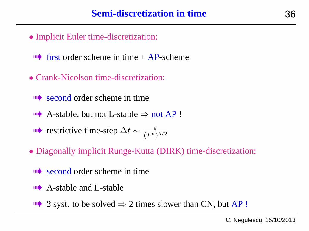
36Semi-discretization in time
• Implicit Euler time-discretization:
first order scheme in time +AP-scheme
• Crank-Nicolson time-discretization:
secondorder scheme in time
A-stable, but not L-stable⇒ not AP!
restrictive time-step∆t ∼ ε(Tn)5/2
• Diagonally implicit Runge-Kutta (DIRK) time-discretization:
secondorder scheme in time
A-stable and L-stable
2 syst. to be solved⇒ 2 times slower than CN, butAP !

C. Negulescu, 15/10/2013
37Numerical results
• Magnetic field: b = B|B| , B =
(
α(2y − 1) cos(πx) + π
πα(y2 − y) sin(πx)
)
• Initial condition: (a) Constr. of analytic solution
(b) Gaussian peak:
T (t = 0, x, y) =Tm2
(
1 + e−50(x−0.5)2−50(y−0.5)2)
,
• Cartesian grids, finite element method (Q2-FEM)
L2-errors between the exact and num. sol. as a function ofε

C. Negulescu, 15/10/2013
38Numerical results
0 0.2 0.4 0.6 0.8 10
0.2
0.4
0.6
0.8
1
x
y(a) ε = 1
0
20
40
60
80
100
0 0.2 0.4 0.6 0.8 10
0.2
0.4
0.6
0.8
1
x
y
(b) ε = 0.5
0
20
40
60
80
0 0.2 0.4 0.6 0.8 10
0.2
0.4
0.6
0.8
1
x
y
(c) ε = 10−1
0
10
20
30
40
50
60
0 0.2 0.4 0.6 0.8 10
0.2
0.4
0.6
0.8
1
x
y
(d) ε = 10−6
0
10
20
30
40
50

C. Negulescu, 15/10/2013
39Closed magnetic field lines
• Magn. field lines:can be closed in real tokamak plasma simulations
⇒ Difficulties in using previous AP-scheme, due to determination of
auxiliary var.qε such that∇||qε =1εT
5/2ε ∇||Tε
L := q ∈ L2(Ω) /∇‖q ∈ L2(Ω) andq|Γin = 0.
• Example of magn. field lines:
B = ∇×(ψ(x, y)ez)+B(x, y)ez , ψ(x, y) = cos(x)+Acos(y−ωt)
−2 −1.5 −1 −0.5 0 0.5 1 1.5 2−4
−3
−2
−1
0
1
2
3
4

C. Negulescu, 15/10/2013
40Asymptotic Preserving method
• Idea:Introduction of astabilization term
(AP )1h
〈∂tTh, vh〉+
∫
Ω(K⊥∇⊥Th) · ∇⊥vh dx+
∫
ΩK‖qh · ∇‖vh dx+ γ
∫
Γ⊥
Thvh ds = 0,
∀vh ∈ Vh∫
ΩK‖T
5/2h ∇‖Th · wh dx− ε
∫
ΩK‖qhwh dx = 0
(AP )2h
〈∂tTh, vh〉+
∫
Ω(K⊥∇⊥Th) · ∇⊥vh dx+
∫
ΩK‖∇‖qh · ∇‖vh dx+ γ
∫
Γ⊥
Thvh ds = 0,
∀vh ∈ Vh∫
ΩK‖T
5/2h ∇‖Th · ∇‖wh dx− ε
∫
ΩK‖∇‖qh · ∇‖wh dx = h3
∫
Ωqhwh dx,
• Advantages:
permits to determine uniquelyqh, without imposing Dirichlet B.C.
on the inflow boundaryΓin
permits to treat closed field lines

C. Negulescu, 15/10/2013
41Numerical results
C. Negulescu, 15/10/2013
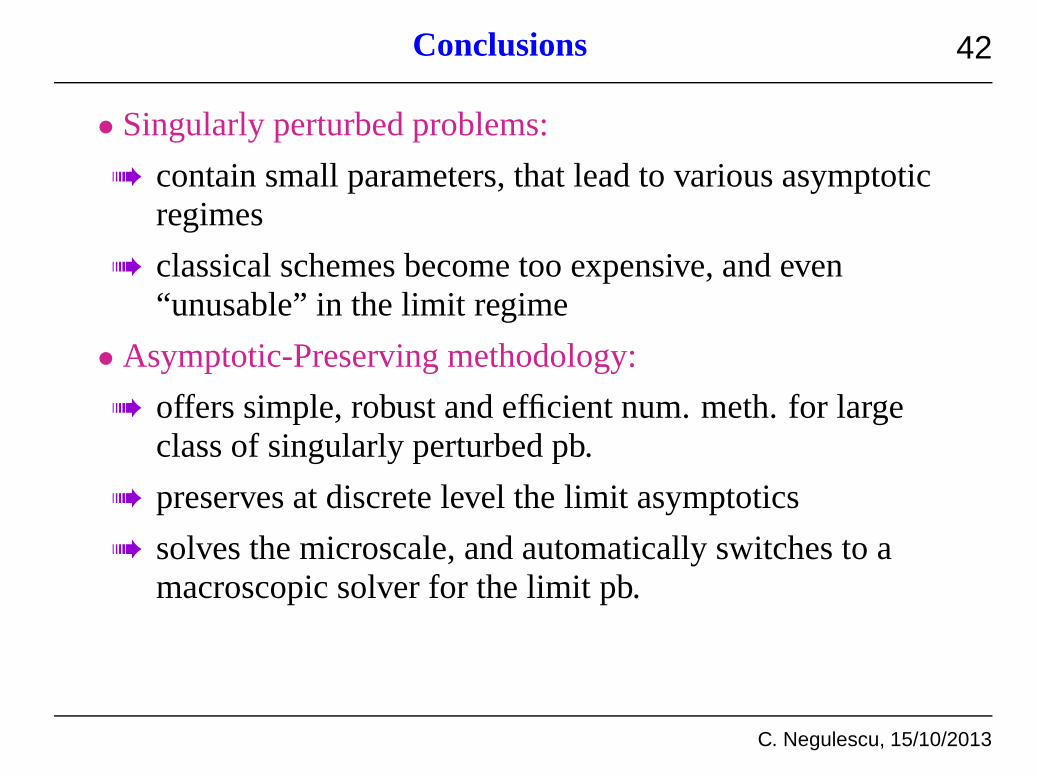
42Conclusions
• Singularly perturbed problems:
contain small parameters, that lead to various asymptoticregimes
classical schemes become too expensive, and even“unusable” in the limit regime
• Asymptotic-Preserving methodology:
offers simple, robust and efficient num. meth. for largeclass of singularly perturbed pb.
preserves at discrete level the limit asymptotics
solves the microscale, and automatically switches to amacroscopic solver for the limit pb.