NASA/CR-2003-212022

Asymptotic

Distribution

of Eigenfrequencies for a Coupled Euler-Bernoulli and Timoshenko Beam Model

Marianna A. ShubovTexas Tech UniversityLubbock, Texas

Cheryl A. PetersonUniversity of California, Los AngelesLos Angeles, California

Under UCLA Grant Number NCC4-121

November 2003

The NASA STI Program Office . . . in Profile

Since its founding, NASA has been dedicatedto the advancement of aeronautics and space science. The NASA Scientific and Technical Information (STI) Program Office plays a keypart in helping NASA maintain thisimportant role.

The NASA STI Program Office is operated byLangley Research Center, the lead center forNASA’s scientific and technical information.The NASA STI Program Office provides access to the NASA STI Database, the largest collectionof aeronautical and space science STI in theworld. The Program Office is also NASA’s institutional mechanism for disseminating theresults of its research and development activities. These results are published by NASA in theNASA STI Report Series, which includes the following report types:

• TECHNICAL PUBLICATION. Reports of completed research or a major significantphase of research that present the results of NASA programs and include extensive dataor theoretical analysis. Includes compilations of significant scientific and technical data and information deemed to be of continuing reference value. NASA’s counterpart of peer-reviewed formal professional papers but has less stringent limitations on manuscriptlength and extent of graphic presentations.

• TECHNICAL MEMORANDUM. Scientificand technical findings that are preliminary orof specialized interest, e.g., quick releasereports, working papers, and bibliographiesthat contain minimal annotation. Does notcontain extensive analysis.

• CONTRACTOR REPORT. Scientific and technical findings by NASA-sponsored contractors and grantees.

• CONFERENCE PUBLICATION. Collected papers from scientific andtechnical conferences, symposia, seminars,or other meetings sponsored or cosponsoredby NASA.

• SPECIAL PUBLICATION. Scientific,technical, or historical information fromNASA programs, projects, and mission,often concerned with subjects havingsubstantial public interest.

• TECHNICAL TRANSLATION. English- language translations of foreign scientific and technical material pertinent toNASA’s mission.

Specialized services that complement the STIProgram Office’s diverse offerings include creating custom thesauri, building customizeddatabases, organizing and publishing researchresults . . . even providing videos.

For more information about the NASA STIProgram Office, see the following:

• Access the NASA STI Program Home Pageat

http://www.sti.nasa.gov

• E-mail your question via the Internet to help@sti.nasa.gov

• Fax your question to the NASA Access HelpDesk at (301) 621-0134

• Telephone the NASA Access Help Desk at(301) 621-0390

• Write to:NASA Access Help DeskNASA Center for AeroSpace Information7121 Standard DriveHanover, MD 21076-1320

NASA/CR-2003-212022

Asymptotic Distribution of Eigenfrequencies for a Coupled Euler-Bernoulli and Timoshenko Beam Model

Marianna A. ShubovTexas Tech UniversityLubbock, Texas

Cheryl A. PetersonUniversity of California, Los AngelesLos Angeles, California

November 2003

National Aeronautics andSpace Administration

Dryden Flight Research CenterEdwards, California 93523-0273

NOTICE

Use of trade names or names of manufacturers in this document does not constitute an official endorsementof such products or manufacturers, either expressed or implied, by the National Aeronautics andSpace Administration.

Available from the following:

NASA Center for AeroSpace Information (CASI) National Technical Information Service (NTIS)7121 Standard Drive 5285 Port Royal RoadHanover, MD 21076-1320 Springfield, VA 22161-2171(301) 621-0390 (703) 487-4650

Asymptotic distribution of eigenfrequencies

for a coupled Euler-Bernoulli and Timoshenko

beam model.

Marianna A. Shubov

Department of Mathematics and StatisticsTexas Tech University, Lubbock, TX 79409

Phone: (806)-742-2336E-mail: marianna.shubov@ttu.edu

Fax: (806)-742-1112

Cheryl A. Peterson

Flight Systems Research CenterDepartment of Electrical Engineering

School of Engineering and Applied SciencesUniversity of California, Los Angeles, CA 90024

Phone: (310)-206-8148

CONTENTS

ABSTRACT . . . . . . . . . . . . . . . . . . . . . . . . . . . . . . . . . . . iv

I. Introduction . . . . . . . . . . . . . . . . . . . . . . . . . . . . . . . . . 1

II. Dynamics Generator and Its General Spectral Properties . . . . 6

2.1 Dynamics Generator . . . . . . . . . . . . . . . . . . . . . . . . . 6

2.2 Operator Setting . . . . . . . . . . . . . . . . . . . . . . . . . . . 7

2.3 Properties of the Dynamics Generator . . . . . . . . . . . . . . 9

III. General Solution of Spectral Equation . . . . . . . . . . . . . . . . 10

3.1 Precise Statement of the Asymptotics of the Spectrum. . . . 10

3.2 Operator Pencil . . . . . . . . . . . . . . . . . . . . . . . . . . . . 11

3.3 Characteristic Equation . . . . . . . . . . . . . . . . . . . . . . . 15

IV. Asymptotic Analysis of the Roots of the Characteristic Polynomial 19

4.1 Cardano’s Formulae . . . . . . . . . . . . . . . . . . . . . . . . . 19

4.2 First Pair of Roots of the Characteristic Equation . . . . . . 25

4.3 Second Pair of Roots of the Characteristic Equation . . . . . 27

4.4 Third Pair of Roots of the Characteristic Equation . . . . . . 29

4.5 General Solution to the Spectral Equation for the

Operator Pencil . . . . . . . . . . . . . . . . . . . . . . . . . . . . . 31

V. The Left–Reflection Matrix . . . . . . . . . . . . . . . . . . . . . . . 32

5.1 Two–step Procedure for Applying Boundary Conditions . . 32

5.2 Left–Reflection Matrix . . . . . . . . . . . . . . . . . . . . . . . . 34

VI. Right–Reflection Matrix . . . . . . . . . . . . . . . . . . . . . . . . 42

VII. Spectral Asymptotics . . . . . . . . . . . . . . . . . . . . . . . . . . . 55

7.1 Spectral Equation. . . . . . . . . . . . . . . . . . . . . . . . . . . 55

7.2 The α–branch of the Spectrum . . . . . . . . . . . . . . . . . . . 58

7.3 The h–branches of the Spectrum . . . . . . . . . . . . . . . . . 60

7.4 Rouche’s Theorem . . . . . . . . . . . . . . . . . . . . . . . . . . 62

VIII.Conclusion . . . . . . . . . . . . . . . . . . . . . . . . . . . . . . . . . . 66

ii

BIBLIOGRAPHY . . . . . . . . . . . . . . . . . . . . . . . . . . . . . . . . . 69

iii

ABSTRACT

This research is devoted to the asymptotic and spectral analysis of a coupled

Euler–Bernoulli and Timoshenko beam model. The model is governed by a system of

two coupled differential equations and a two parameter family of boundary conditions

modelling the action of self–straining actuators. The aforementioned equations of

motion together with a two–parameter family of boundary conditions form a coupled

linear hyperbolic system, which is equivalent to a single operator evolution equation

in the energy space. That equation defines a semigroup of bounded operators. The

dynamics generator of the semigroup is our main object of interest. For each set

of boundary parameters, the dynamics generator has a compact inverse. If both

boundary parameters are not purely imaginary numbers, then the dynamics generator

is a nonselfadjoint operator in the energy space. We calculate the spectral asymptotics

of the dynamics generator. We find that the spectrum lies in a strip parallel to the

horizontal axis, and is asymptotically close to the horizontal axis – thus the system

is stable, but is not uniformly stable.

iv

CHAPTER I

Introduction

We study the spectral properties and derive the spectral asymptotics of a family

of nonselfadjoint operators generated by a coupled Euler–Bernoulli and Timoshenko

beam model. Such a model actually occurs in classical aeroelastic textbooks such

as [1,2,3]. We formulate and prove spectral asymptotics of nonselfadjoint operators

that are the dynamics generators for hyperbolic systems, which govern the motion of

a coupled Euler–Bernoulli and Timoshenko beam model subject to a two–parameter

family of nonconservative boundary conditions. The specific model that we consider

includes a two parameter family of boundary conditions which model the action of

piezo–electric materials. The precise formulation of the problem and its partial anal-

ysis are presented in paper [4].

Before we turn to the description of the model and outline the main findings in

this research, we would like to emphasize the connection between the present math-

ematical study and the problem of flutter analysis of an aircraft wing in a subsonic

air flow. The model discussed in this paper describes the so–called ground vibrations

of a long and slender aircraft wing. Such a problem is the first step in the analysis

of a response of an aircraft wing to the turbulent air flow when an aircraft is in–

flight. The problem of ground vibrations has been known for a long time. However,

an extensive mathematical and engineering literature related to the problem (often

called the bending–torsion vibration model) deals either with numerical calculations

or experimental verification of the numerical results. Analytical investigation of the

properties of the vibrating coupled beams with nonconservative boundary conditions

has been, in fact, an open problem. In the present paper, we present the first in the

literature on aeroelasticity analytical formulae for the eigenfrequencies of the ground

vibrations. Such an important step forward in the study of this problem has become

possible not only due to the mathematical and physical backgrounds of the authors,

1

but also due to two additional special reasons. Namely, the major part of the analysis

has been accomplished when the first author (M.A. Shubov) has been awarded with

Interdisciplinary Grant in the Mathematical Sciences (IGMS) by the National Sci-

ence Foundation (NSF Award Number: 9972748; Amount: $100,000; Initial period:

09/01/99–08/31/00; Extension with Expiration Date: 08/31/01). Due to this award,

the first author had a one–year visit to Flight Systems Research Center (FSRC) at

UCLA. During this stay at FSRC, the first author was able to acquire substantial

knowledge in the area of aircraft engineering while working together with the research

team of the Center and by discussing different topics with the Director of FSRC, Prof.

A.V. Balakrishnan. In addition to the research, done on the problem and presented in

this paper, the author was able to create a basis for future research on mathematical

problems arising in aircraft engineering.

The second author (C.A. Peterson) participated in this study as a graduate student

of Dr. M.A. Shubov. For her research, the second author has been awarded with two

Texas Space Grant Consortium Fellowships (in 2000–2001 and in 2001–2002 school

years). At the school year 2002–2003, the second author is a Post–graduate Research

Engineer at FSRC (UCLA), where she is working on numerical simulations to verify

the efficiency of the spectral asymptotics obtained analytically in the present paper.

Now we briefly describe the organization of the paper.

• In Chapter I, we introduce a coupled system of differential equations, which will be

our main system in the present work. We also introduce a two–parameter family of

boundary conditions, which contains two control parameters (see also [5, 6]).

• In Chapter II, we justify the new setting of the initial boundary–value problem in

the form of the first order in time evolution equation. The asymptotic properties of

the spectrum of the dynamics generator is our main interest in the work.

• In Chapter III, we initiate methodical study of the spectrum of the dynamics gen-

erator. As the first step, we reduce the problem for the spectrum of the generator to

the problem of finding spectral asymptotics for the corresponding operator pencil. We

recall the definitions related to operator pencils and provide the explanation why the

2

pencil considered in the present work is highly nonstandard and extremely compli-

cated. We show that the first necessary step is to analyze the asymptotic behavior of

the fundamental system of solutions of the sixth order ordinary differential equation

involving the spectral parameter λ (see Eq.(3.16) below). The latter analysis requires

us to derive asymptotics for the roots of the sixth order polynomial of a special type.

• In Chapter IV, we derive asymptotic approximations for the roots of the charac-

teristic polynomial, which is associated to the aforementioned sixth order ordinary

differential equation. Namely, we obtain the approximations for six roots of the sixth

order polynomial, approximations when the spectral parameter |λ| → ∞ and those

approximations are uniform with respect to the spatial variable x. Technically, this

Chapter is very complicated and the results obtained in it are of crucial importance

for the remaining Chapters V–VIII.

• In Chapter V, we introduce a special method to solve the boundary problem, i.e.,

we use the so–called two–step procedure. This is a relatively new method that has

been introduced in papers [7–9] to solve the boundary–value problem for a spatially

nonhomogeneous Timoshenko beam model. By using the aforementioned procedure,

we examine the effect of applying the boundary conditions from the left and from

the right separately. Namely, in Section 5.2, we look for a solution of the spectral

equation for the operator pencil, a solution which satisfies only three left–hand side

boundary conditions without any restrictions on the behavior of such a solution at the

right–hand side of the flexible structure. In this Section, we introduce an important

notion which we call the left–reflection matrix and denote it as Rl.

• In Chapter VI, we derive an asymptotic approximation for the right–reflection ma-

trix, which is similar to the left–reflection matrix of Chapter V. The right reflection

matrix is useful to describe the solution of the main differential equation, which sat-

isfies only the right–hand side boundary conditions without imposing any restrictions

on the solution at the left end.

• In Chapter VII, we incorporate all information obtained in the previous two Chap-

ters to derive the spectral asymptotics. The main tool in proving asymptotical for-

3

mulae (3.2)–(3.3) with the necessary accuracy is the well–known Rouche’s Theorem.

Euler–Bernoulli/Timoshenko Beam Model

From now on, we will focus on the boundary–value problem consisting of a system

of two coupled hyperbolic partial differential equations in two unknown functions h

and α, with h(t, x) being a deflection at a point x at a time moment t and α(t, x)

being a torsion angle at a point x and a time t. We assume that the spatial extent of

the flexible structure is L and t > 0.

mh(t, x) + Sα(t, x) + EIh′′′′

(t, x) = 0, −L < x < 0; 0 < t,

Sh(t, x) + Iαα(t, x)−GJα′′(t, x) = 0, −L < x < 0; 0 < t,

(1.1)

where m is a mass per unit length, S is a mass moment per unit length, EI is a

bending stiffness, GJ is a torsion stiffness, and Iα is a moment of inertia. The system

is supplied with a two–parameter family of boundary conditions

h(t,−L) = h′(t,−L) = 0 α(t,−L) = 0; (1.2)

h′′′(t, 0) =0,

EIh′′(t, 0) + ghh′(t, 0) =0,

GJα′(t, 0) + gαα(t, 0) =0.

(1.3)

In (1.1)–(1.3), we have denoted the time derivative by the over dot.

We notice now that the set of boundary conditions at the left end is standard.

However, the right–hand side boundary conditions are highly nonstandard, i.e., they

contain two arbitrary parameters gh and gα. These parameters are used in current

mathematical and engineering literature in order to model the action of “smart ma-

terials” (see [10–13]). Technically, the analysis can be carried out for any complex

values of the boundary parameters. An important case for practical applications is

4

the one when gh and gα are positive numbers. In this case, gh is called a bending

control gain and gα is called a torsion control gain.

In addition to the boundary conditions, we introduce a set of initial conditions in

a standard manner

h(0, x) = h0(x), h(t, x)∣∣t=0

= h1(x), α(0, t) = α0(x), α(t, x)∣∣t=0

= α1(x). (1.4)

To conclude the Introduction, we note that we consider a beam that is perfectly

elastic, and rigid in cross sections perpendicular to the lengthwise direction. It has an

elastic axis, implying that the wing is unswept and without structural discontinuities,

so that elastic coupling between bending and twisting is eliminated. The elastic axis

is straight, and rotary inertia and shear deformation is neglected.

5

CHAPTER II

Dynamics Generator and Its General Spectral Properties

2.1 Dynamics Generator

To analyze the initial boundary–value problem (1.1)–(1.3), we will present it as a

first order in time evolution equation. The dynamics generator will be our main object

of interest. We will show that the dynamics generator is a 4 × 4 matrix differential

operator, which acts in the so–called energy space. To introduce the formula for

the dynamics generator and to describe its domain, we carry out the following steps.

First, we can verify that our system of equations

mh(t, x) + Sα(t, x) = −EIh′′′′

(t, x),

Sh(t, x) + Iαα(t, x) = GJα′′(t, x).

(2.1)

can be represented in the form

1 0 0 0

0 1 0 0

0 0 m S

0 0 S Iα

h(t, x)

α(t, x)

h(t, x)

α(t, x)

=

0 0 1 0

0 0 0 1

−EI∂4

∂x40 0 0

0 GJ∂2

∂x20 0

h(t, x)

α(t, x)

h(t, x)

α(t, x)

. (2.2)

If we introduce a 4–component vector Y by the formula Y = (h, α, h, α)T (the

superscript “T” means transposition), and denote the matrices in (2.2) by M and A,

then Eq.(2.2) can be written in the form

MY = AY. (2.3)

Now we introduce an important assumption

∆ = mIα − S2 > 0. (2.4)

Due to (2.4), we can rewrite Eq.(2.3) as

Y = M−1AY = i[−iM−1A]Y. (2.5)

6

Denoting L = −iM−1A, we finally rewrite Eq.(2.5) in the desired form

Y = iLY. (2.6)

If ΦT (t, x) = {φ0(t, x), φ1(t, x), φ2(t, x), φ3(t, x)} = {h, α, h, α}, −L ≤ x ≤ 0,

t ≥ 0, then the initial–boundary value problem (1.1)–(1.3) can be rewritten in the

form of the first order in time evolution equation

Φ = iLΦ, Φ∣∣t=0

= Φ0, (2.7)

with the dynamics generator L being defined on smooth functions Φ = (φ0, φ1, φ2, φ3)T

by the formula

L = −i

0 0 1 0

0 0 0 1

−IαEI

∆

∂4

∂x4

−S GJ

∆

∂2

∂x20 0

S EI

∆

∂4

∂x4

mGJ

∆

∂2

∂x20 0

. (2.8)

subject to the following boundary conditions:

φ0(−L) = φ′0(−L) = φ1(−L) = 0,,

φ′′′0 (0) = 0,

EIφ′′0(0) + ghφ′2(0) = 0,

GJφ′1(0) + gαφ3(0) = 0.

(2.9)

2.2 Operator Setting

Let us consider the energy of the system by carrying out the following steps.

Let us multiply the first equation from system (2.1) by ht and the second equation

from system (2.1) by αt and then add the resulting two equations. If we denote the

resulting sum as EQ1, we have

EQ1 = mhtt(t, x)ht(t, x) + Sαtt(t, x)ht(t, x) + EI h′′′′(t, x)ht(t, x)+

Shtt(t, x)αt(t, x) + Iααtt(t, x)αt(t, x)−GJ α′′(t, x)αt(t, x) = 0.(2.10)

7

Let us take the complex conjugate of Eq.(2.10) and denote this equation by EQ2. It

can be verified by a direct calculation that we have the following result:

EQ1 + EQ2 = md

dt|ht(t, x)|2 + S

d

dt

(αt(t, x)ht(t, x) + αt(t, x)ht(t, x)

)+

EI(h′′′′(t, x)ht(t, x) + h

′′′′(t, x)ht(t, x)

)+ Iα

d

dt|αt(t, x)|2−

GJ (α′′(t, x)αt(t, x) + α′′(t, x)αt(t, x)) = 0.

(2.11)

Eq.(2.11) suggests that a convenient expression for the energy of the system can be

taken in the form of the following functional:

E(t) =1

2

∫ 0

−L

[EI |h′′(t, x)|2 + GJ |α′(t, x)|2 + m |ht(t, x)|2 +

Iα |αt(t, x)|2 + S(αt(t, x)ht(t, x) + αt(t, x)ht(t, x)

)]dx.

(2.12)

The following Lemma regarding this energy has been proved in our paper [14].

Lemma 2.1. Under condition (2.4), the energy of vibrations, given by formula

(2.12), is nonnegative and is equal to zero if and only if h(t, x) = α(t, x) = 0,

x ∈ [−L, 0], t ≥ 0.

With this energy of vibrations, we can define the operator setting of the problem.

First we describe the state space of the system, which will be denoted by H. Let Hbe a set of 4–component vector–valued functions Φ = (φ0, φ1, φ2, φ3)

T obtained as a

closure of smooth functions satisfying the conditions

φ0(−L) = φ′0(−L) = φ1(−L) = 0 (2.13)

in the following energy norm:

‖Φ‖2H =

1

2

∫ 0

−L

[EI |φ′′0(x)|2 + GJ |φ′1(x)|2 + m |φ2(x)|2 + Iα |φ3(x)|2 +

S(φ2(x)φ3(x) + φ2(x)φ3(x)

)]dx.

(2.14)

This is shown to be a norm in our paper [14]. The operator L is given by formula

8

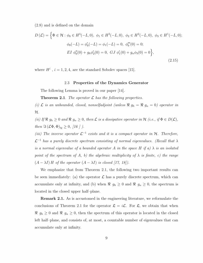
(2.8) and is defined on the domain

D (L) ={

Φ ∈ H : φ0 ∈ H4(−L, 0), φ1 ∈ H2(−L, 0), φ2 ∈ H2(−L, 0), φ3 ∈ H1(−L, 0);

φ0(−L) = φ′0(−L) = φ1(−L) = 0, φ′′′0 (0) = 0;

EI φ′′0(0) + ghφ′2(0) = 0, GJ φ′1(0) + gαφ3(0) = 0

},

(2.15)

where H ι , ι = 1, 2, 4, are the standard Sobolev spaces [15].

2.3 Properties of the Dynamics Generator

The following Lemma is proved in our paper [14].

Theorem 2.1. The operator L has the following properties.

(i) L is an unbounded, closed, nonselfadjoint (unless < gh = < gα = 0) operator in

H.

(ii) If < gh ≥ 0 and < gα ≥ 0, then L is a dissipative operator in H (i.e., if Φ ∈ D(L),

then = (LΦ, Φ)H ≥ 0, [16 ] ).

(iii) The inverse operator L−1 exists and it is a compact operator in H. Therefore,

L−1 has a purely discrete spectrum consisting of normal eigenvalues. (Recall that λ

is a normal eigenvalue of a bounded operator A in the space H if a) λ is an isolated

point of the spectrum of A, b) the algebraic multiplicity of λ is finite, c) the range

(A− λI) H of the operator (A− λI) is closed [17, 18]).

We emphasize that from Theorem 2.1, the following two important results can

be seen immediately: (a) the operator L has a purely discrete spectrum, which can

accumulate only at infinity, and (b) when < gh ≥ 0 and < gα ≥ 0, the spectrum is

located in the closed upper half–plane.

Remark 2.1. As is accustomed in the engineering literature, we reformulate the

conclusions of Theorem 2.1 for the operator L = iL. For L, we obtain that when

< gh ≥ 0 and < gα ≥ 0, then the spectrum of this operator is located in the closed

left half–plane, and consists of, at most, a countable number of eigenvalues that can

accumulate only at infinity.

9

CHAPTER III

General Solution of Spectral Equation

3.1 Precise Statement of the Asymptotics of the Spectrum.

We formulate now a precise statement of the spectral results, which will be proven

in the rest of the paper.

Theorem 3.1. (a) The operator L has a countable set of complex eigenvalues.

Under the assumption

gα 6=√

Iα GI, (3.1)

the set of eigenvalues is located in a strip parallel to the real axis.

(b) The entire set of the eigenvalues asymptotically splits into two disjoint subsets. We

call them the h–branch and the α–branch and denote these branches by {λhn}n∈Z and

{λαn}n∈Z respectively. If < gα ≥ 0 and < gh > 0, then the α–branch is asymptotically

close to some horizontal line in the upper half–plane. If < gh = < gα = 0, then the

operator L is selfadjoint and thus its spectrum is real. The entire set of eigenvalues

may have only two points of accumulation: +∞ and −∞ in the sense that < λh(α)n →

±∞ and = λh(α)n < const as n → ±∞ (see formulae (3.2) and (3.3) below).

(c) The following asymptotic formula is valid for the h–branch of the spectrum:

λhn = ±π2/L2

√IαEI/∆(|n| − 1/4)2 + O(1), |n| → ∞. (3.2)

In formula (3.2), the sign “+” should be taken for n > 0 and “−” for n < 0.

(d) The following asymptotic formula is valid for the α–branch of the spectrum:

λαn =

πn

L√

Iα/GJ+

i

2L√

Iα/GJln

gα +√

Iα GJ

gα −√

Iα GJ+ O(|n|−1/2), |n| → ∞. (3.3)

In (3.3), the principle value of the logarithm is understood.

10

3.2 Operator Pencil

In this section, we introduce an operator–valued polynomial function, which we

call an operator pencil. To introduce this operator pencil, which is associated to the

dynamics generator L, we start with the spectral equation for this operator

LΦ = λΦ, Φ ∈ D(L). (3.4)

Using the explicit formula for L, we obtain

−i

0 0 1 0

0 0 0 1

−IαEI

∆

∂4

∂x4

−S GJ

∆

∂2

∂x20 0

S EI

∆

∂4

∂x4

mGJ

∆

∂2

∂x20 0

φ0

φ1

φ2

φ3

= λ

φ0

φ1

φ2

φ3

. (3.5)

Rewriting Eq.(3.5) component–wise yields the following four equations:

φ2 = iλφ0, (3.6)

φ3 = iλφ1, (3.7)

IαEI

∆φIV

0 +S GJ

∆φ′′1 = −iλφ2, (3.8)

S EI

∆φIV

0 +mGJ

∆φ′′1 = iλφ3. (3.9)

Our goal is to eliminate the three components φ1, φ2, and φ3 from system (3.6)–(3.9)

and to derive a single equation with respect to the one component φ0. Substituting

Eqs.(3.6) and (3.7) into Eqs.(3.8) and (3.9) to eliminate φ2 and φ3, we obtain

Iα EI φIV0 + S GJ φ′′1 = ∆λ2φ0, (3.10)

S EIφIV0 + mGJφ′′1 = −∆λ2φ1, (3.11)

where ∆ is defined in (2.4). We will now eliminate φ1 from Eqs. (3.10) and (3.11).

To this end, let us solve Eq.(3.10) for φ′′1 and obtain

φ′′1 =1

S GJ[−IαEIφIV

0 + λ2∆φ0]. (3.12)

11

Differentiating both sides of the latter equation gives

φIV1 =

1

S GJ[−IαEIφV I

0 + λ2∆φ′′0]. (3.13)

By twice differentiating both sides of Eq.(3.11), we obtain

S EIφV I0 + mGJφIV

1 = −λ2∆φ′′1. (3.14)

Substituting (3.12) and (3.13) into Eq.(3.14) and multiplying both sides by S GJ

gives

S2 GJ EIφV I0 + mGJ [−IαEIφV I

0 + λ2∆φ′′0] = λ2∆[IαEIφIV0 − λ2∆φ0]. (3.15)

Collecting like terms in Eq.(3.15) and then simplifying, we arrive at the following

final form of the equation for the component φ0:

EI GJφV I0 + λ2IαEIφIV

0 − λ2m GJφ′′0 − λ4∆φ0 = 0. (3.16)

Thus, we have defined an equation, in which φ0 and its derivatives are the only

unknown functions. We notice that the left–hand side of Eq.(3.16) is a fourth order

polynomial with respect to λ. However, coefficients in that polynomial are high

order differential operations. It is convenient to introduce special notation for this

operation.

Let P(·) be a polynomial operation defined by the formula

P(λ)φ0 = EI GJφV I0 + λ2IαEIφ

′′′′0 − λ2mGJφ′′0 − λ4∆φ0, (3.17)

where φ0 is a smooth function for x ∈ [−L, 0]. In order to determine the domain of

P(·), we have to calculate the conditions, which φ0 inherits from the domain of the

operator L. To do this, we will take the boundary conditions from the domain of the

dynamics generator L (see 2.9) and rewrite them in terms of φ0 and its derivatives.

First of all, we need to write φ1 in terms of φ0. To carry out this elimination, we return

to the system of two equations (3.10) and (3.11). From this system of two equations,

we will eliminate φ′′1 to obtain one equation involving φ0 and its derivatives and φ1

12

which will then be solved for. We will accomplish the following sequence of steps:

first, we divide Eq.(3.10) by S and Eq.(3.11) by m; secondly, we subtract the second

equation from the first one and have

φIV0

[Iα EI

S− S EI

m

]=

∆λ2

Sφ0 +

∆λ2

mφ1. (3.18)

Simplifying Eq.(3.18) and taking into account formula (2.4) for ∆, we obtain the

representation for φ1 in terms of φ0

φ1 =EI

Sλ−2φIV

0 − m

Sφ0. (3.19)

This expression for φ1 will be substituted along with (3.6) and (3.7), into the boundary

conditions (2.9) to obtain precise boundary conditions needed for the function φ0 to

be in the domain of the operator pencil.

The first two boundary conditions, being only in terms of φ0, remain unchanged,

i.e., we have φ0(−L) = 0 and φ′0(−L) = 0. Substituting (3.19) into the third boundary

condition yields

EIφIV0 (−L)− λ2mφ0(−L) = 0. (3.20)

So far, we have determined the left–hand boundary conditions. Now we derive

appropriate forms for the right–hand boundary conditions. The fourth boundary

condition of (2.9), being only in terms of φ0, remains the same, i.e. φ′′′0 (0) = 0. The

fifth boundary condition of (2.9), after substitution of (3.6), becomes

EIφ′′0(0) + iλghφ′0(0) = 0. (3.21)

The only boundary condition that remains to be determined is the sixth one. This

condition after substitution of (3.7) becomes

GJφ′1(0) + iλgαφ1(0) = 0. (3.22)

Replacing φ1 according to formula (3.19) leads to

GJ

[EI

Sλ−2φV

0 (0)− m

Sφ′0(0)

]+ gαiλ

[EI

Sλ−2φIV

0 (0)− m

Sφ0(0)

]= 0. (3.23)

13

Multiplying Eq.(3.23) by Sλ2 and rearranging its terms, we arrive at the following

boundary condition:

EI GJ φV0 (0) + iλEI gαφIV

0 (0)− λ2m GJ φ′0(0)− iλ3gαmφ0(0) = 0. (3.24)

Therefore, the problem of finding the eigenvalues and eigenfunctions of the op-

erator L (see Eq.(3.5)) has been reduced to the problem of finding those values of

the parameter λ for which the sixth order ordinary differential equation (3.16) has

nontrivial solutions satisfying six boundary conditions.

Now we are in a position to introduce a pencil associated with the operator L.

We recall [19] that a polynomial operator pencil A(λ) is an operator–valued function

defined by the formula A(λ) = λn + λn−1An−1 + ... + A0 in which Ak are linear op-

erators. Those operators may be either bounded or unbounded and either selfadjoint

or nonselfadjoint. The degree n of this polynomial is called the order of the pencil.

Let P(·) be the fourth order operator pencil that acts on a function φ ∈ H6(−L, 0)

by the formula

P(λ)φ = EI GJφV I + λ2IαEIφIV − λ2mGJφ′′ − λ4∆φ (3.25)

and is defined on the domain

D(P) = {φ ∈ H6(−L, 0) : φ(−L) = φ′(−L) = φIV (−L) = 0;

EIφ′′(0) + ghiλφ′(0) = 0, φ′′′(0) = 0,

EI GJ φV (0) + EI gαiλφIV (0)−mGJ λ2φ′(0)− gαmiλ3φ(0) = 0}.

(3.26)

We note that H6 is the standard Sobolev space [15]. We call a nontrivial solution

φ ∈ D(P) of the pencil equation P(λ)φ = 0 an eigenfunction of the pencil P(·)and the corresponding value of λ an eigenvalue of P(·). It is clear that having an

eigenfunction of the pencil and using (3.19), we can find φ1 and then find all four

components of the eigenvector of the operator L.

We mention that P(·) is a nonstandard pencil due to the fact that the spectral

parameter λ enters the domain explicitly. These type of pencils have not been con-

sidered in the monograph [19]. However, it is convenient to keep the terminology

14

because there exists an extensive literature in which the pencils with the parameter

dependent boundary conditions appear naturally.

3.3 Characteristic Equation

In this section, we initiate the analysis of the pencil equation P(λ)φ = 0. In

particular, in the present section we focus on the differential equation (3.16), which

is a sixth order ordinary differential equation with constant coefficients containing

the complex parameter λ. We are looking for the asymptotic representation for the

fundamental system of its solutions. It is important to mention that we are looking

for the asymptotics with respect to λ when |λ| → ∞ and those asymptotics must be

uniform with respect to the spatial variable x ∈ [−L, 0].

As is well–known, to find the fundamental system of solutions of the sixth order

ordinary differential equation, we have to find appropriate approximations for the

roots of the sixth order polynomial, which is the characteristic polynomial for the

differential equation. The characteristic equation has the following form:

EI GJ(x2)3 + λ2Iα EI(x2)2 − λ2mGJ(x2)−∆λ4 = 0. (3.27)

Clearly, Eq.(3.27) is of a sixth order, but if we change an independent variable, we

can reduce it to a cubic equation. Namely, let

y = x2, (3.28)

and then rewriting Eq.(3.27) in terms of y, we have

EI GJy3 + λ2Iα EIy2 − λ2mGJy −∆λ4 = 0. (3.29)

Using Cardano’s Formulae [20], we can obtain the solution of a cubic polynomial.

However, in order to apply those formulae, we need the cubic polynomial to be monic

with no quadratic term. Let us reduce the polynomial in (3.29) to the desired form.

Dividing both sides of (3.29) by EI GJ yields

y3 +

(Iαλ2

GJ

)y2 −

(mλ2

EI

)y − ∆λ4

EI GJ= 0, (3.30)

15

which is a monic polynomial. Next we need to make the quadratic term in (3.30)

vanish. To do so, we notice that for a polynomial such as

f(x) = x3 + a2x2 + a1x + a0, (3.31)

the substitution

x = z − a2/3 (3.32)

will result in a polynomial in z, with no quadratic term [20]. So if we substitute

y = z − 1

3

(Iα

GJλ2

)(3.33)

into Eq.(3.30), then we have an equation adjusted to Cardano’s Formulae. Taking

into account that

y3 = y(y2) =

(z − Iαλ2

3GJ

) (z2 − 2Iαλ2

3GJz +

(Iαλ2

3GJ

)2)

= z3 − Iαλ2

GJz2 +

1

3

(Iαλ2

GJ

)2

z −(

Iαλ2

3GJ

)3

,

(3.34)

and substituting (3.33) and (3.34) into Eq.(3.30), we obtain

[z3 − Iαλ2

GJz2 +

1

3

(Iαλ2

GJ

)2

z −(

Iαλ2

3GJ

)3]

Iαλ2

GJ

[z2 − 2Iαλ2

3GJz +

(Iαλ2

3GJ

)2]−

(mλ2

EI

)[z − 1

3

(Iαλ2

GJ

)]− ∆λ4

EI GJ= 0,

(3.35)

and cancel the two quadratic terms as expected. Then we combine same powers of z

and have

z3 +

[1

3

(Iαλ2

GJ

)2

− 2

3

(Iαλ2

GJ

)2

− mλ2

EI

]z+

[−

(Iαλ2

3GJ

)3

+1

32

(Iαλ2

GJ

)3

+1

3

(mλ2

EI

)(Iαλ2

GJ

)− ∆λ4

EI GJ

]= 0.

(3.36)

16

Simplifying the coefficients in Eq.(3.36), we finally obtain the monic cubic polynomial

with no quadratic term as

z3 −[

1

3

(Iαλ2

GJ

)2

+mλ2

EI

]z +

[2

(Iαλ2

3GJ

)3

+Iαm− 3∆

3EI GJλ4

]= 0. (3.37)

It is this polynomial that we will apply Cardano’s Formulae to in the next section.

We recall that our goal is to find asymptotic approximations for six roots of

Eq.(3.27) when |λ| → ∞. However, before proceeding to find the six roots, we will

see what knowledge may be gained by investigating the asymptotic behavior of the

solutions of a simpler equation than Eq.(3.37). We will call this simpler equation the

model equation. Let us rewrite Eq.(3.37) in the asymptotical form as |λ| → ∞.

z3 − λ4

3

(Iα

GJ

)2

(1 + O(λ−2))z + λ6 2I3α

33(GJ)3(1 + O(λ−2) = 0. (3.38)

By omitting the lower order terms O(λ−2) in Eq.(3.35), we obtain the model equation

z3 − λ4

3

(Iα

GJ

)2

z + λ6 2I3α

33(GJ)3= 0. (3.39)

Assuming that a solution z1 will be a multiple of λ2, we substitute

z1 = aλ2 (3.40)

into Eq.(3.39) and divide by λ6 to obtain a cubic equation for the multiple a

a3 −(

Iα

GJ

)21

3a +

2

33

(Iα

GJ

)3

= 0, (3.41)

from which we guess that a solution a will be a multiple of Iα/GJ . So, now making

the substitution a = bIα/GJ and then dividing by (Iα/GJ)3 yields

b3 − 1

3b +

2

33= 0. (3.42)

One can check directly that a solution of this equation is b = 1/3. Thus we find that

one solution z1 of the model equation (3.39) can be found by successive substitutions

into (3.40) as follows:

z1 = aλ2 =Iαλ2

3GJ= λ2R

3, (3.43)

17

where

R =Iα

GJ. (3.44)

Factoring the model equation yields

(z − Iαλ2

3GJ

) (z2 +

Iαλ2

3GJz − 2

9

(Iα

GJ

)2

λ4

)= 0. (3.45)

The roots of the quadratic polynomial (3.45) are

z2 =1

3

(Iα

GJ

)λ2, z3 = −2

3

(Iα

GJ

)λ2. (3.46)

Thus we have the following three solutions to the model equation:

z1 = z2 =Iαλ2

3GJ, z3 = −2

3

(Iα

GJ

)λ2. (3.47)

Note that z1 = z2. From the latter fact, we can expect that two roots of Eq.(3.37)

will have a similar behavior in nature, while the third solution will behave differently.

This exact difference in behavior remains to be seen.

18

CHAPTER IV

Asymptotic Analysis of the Roots of the Characteristic

Polynomial

4.1 Cardano’s Formulae

It is well–known, Cardano’s Formulae [20] give a solution for a monic cubic equa-

tion with no quadratic term such as

z3 + pz + q = 0, (4.1)

where p and q are constants. The solution given by Cardano’s Formulae to Eq.(4.1)

can be represented in the form

z = u− v, (4.2)

where

u =3

√−q

2+

√(q

2

)2

+(p

3

)3

, v =3

√q

2+

√(q

2

)2

+(p

3

)3

. (4.3)

We will use formulae (4.2) and (4.3) to find solutions to the characteristic equation

(3.27). Recall that we made substitution (3.28) that

x2 = y, (4.4)

to obtain a cubic polynomial. Next we substituted the shift of (3.32) to obtain a

cubic equation with no quadratic term. Making this substitution into (4.4) gives us

x2 = z − λ2Iα

3 GJ. (4.5)

When we apply the Cardano Formulae to this z using (4.2), we will have that

x2 = u− v − λ2Iα

3 GJ. (4.6)

Solving for x, we find the first pair of solutions of the characteristic equation (3.27)

x1,2 = ±√

u− v − λ2Iα

3 GJ, (4.7)

19

where u and v are as in (4.3) and the p and q in these expressions can be found upon

comparison of (4.1) with (3.37).

We now proceed to make the necessary preliminary calculations. Upon inspection

of (4.3), we find that we need to calculate (q/2)2, (p/3)3. For (q/2)2 we have

(q

2

)2

=

(Iα

3GJ

)6

λ12 +I3α(Iαm− 3∆)

34EI(GJ)4λ10 +

(Iαm− 3∆

6EI GJ

)2

λ8, (4.8)

where q was found from (3.37). Similarly we obtain p from (3.37) and calculate

(p

3

)3

= −[(

Iα

3GJ

)6

λ12 +

(Iα

3GJ

)4 ( m

EI

)λ10

+1

3

(Iα

3GJ

)2 ( m

EI

)2

λ8 +( m

3EI

)3

λ6

].

(4.9)

Finally, we sum (4.8) and (4.9) and simplify as follows:

(q

2

)2

+(p

3

)3

=

[I3α(Iαm− 3∆)

34EI(GJ)4− I4

αm

34EI(GJ)4

]λ10

+

[(Iαm− 3∆

6EI GJ

)2

− 1

3

(Iα

3GJ

)2 ( m

EI

)2]

λ8 −( m

3EI

)3

λ6

=− I3α∆

33EI(GJ)4λ10 − I2

αm2 + 18Iαm∆− 27∆2

334(EI GJ)2λ8 −

( m

3EI

)3

λ6.

(4.10)

Notice that the terms containing λ12 cancelled each other out. By simplifying the

second term’s numerator, we have

I2αm2 + 18Iαm∆− 33∆2 = I2

αm2 + 18Iαm(Iαm− S2)− 33(Iαm− S2)2

= −8I2αm2 + 36IαmS2 − 33S4.

(4.11)

20

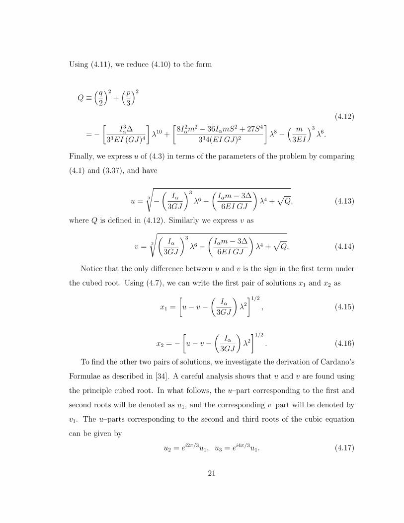
Using (4.11), we reduce (4.10) to the form

Q ≡(q

2

)2

+(p

3

)2

=−[

I3α∆

33EI (GJ)4

]λ10 +

[8I2

αm2 − 36IαmS2 + 27S4

334(EI GJ)2

]λ8 −

( m

3EI

)3

λ6.

(4.12)

Finally, we express u of (4.3) in terms of the parameters of the problem by comparing

(4.1) and (3.37), and have

u =3

√−

(Iα

3GJ

)3

λ6 −(

Iαm− 3∆

6EI GJ

)λ4 +

√Q, (4.13)

where Q is defined in (4.12). Similarly we express v as

v =3

√(Iα

3GJ

)3

λ6 −(

Iαm− 3∆

6EI GJ

)λ4 +

√Q, (4.14)

Notice that the only difference between u and v is the sign in the first term under

the cubed root. Using (4.7), we can write the first pair of solutions x1 and x2 as

x1 =

[u− v −

(Iα

3GJ

)λ2

]1/2

, (4.15)

x2 = −[u− v −

(Iα

3GJ

)λ2

]1/2

. (4.16)

To find the other two pairs of solutions, we investigate the derivation of Cardano’s

Formulae as described in [34]. A careful analysis shows that u and v are found using

the principle cubed root. In what follows, the u–part corresponding to the first and

second roots will be denoted as u1, and the corresponding v–part will be denoted by

v1. The u–parts corresponding to the second and third roots of the cubic equation

can be given by

u2 = ei2π/3u1, u3 = ei4π/3u1. (4.17)

21

The v–parts corresponding to the second and third roots of the cubic equation

can be given by

v2 = e−i2π/3v1, v3 = e−i4π/3v1. (4.18)

Substituting these results in the formulae similar to (4.7) gives us formulae for the

other four solutions to the characteristic equation. We present below the formulae

for the remaining four roots of the characteristic equation

x3 =

[ei2π/3u1 − e−i2π/3v1 −

(Iα

3GJ

)λ2

]1/2

, (4.19)

x4 = −[ei2π/3u1 − e−i2π/3v1 −

(Iα

3GJ

)λ2

]1/2

, (4.20)

x5 =

[ei4π/3u1 − e−i4π/3v1 −

(Iα

3GJ

)λ2

]1/2

, (4.21)

and

x6 = −[ei4π/3u1 − e−i4π/3v1 −

(Iα

3GJ

)λ2

]1/2

. (4.22)

Recall that the exponentials in the formulae for the roots can be written as

ei2π/3 = −1

2+ i

√3

2= e−i4π/3, ei4π/3 = −1

2− i

√3

2= e−i2π/3, (4.23)

and these alternate expressions will be used for later calculations.

We could easily make all necessary substitutions into (4.7) and (4.19)–(4.22) to

obtain exact solutions to the characteristic equation in terms of the parameters of the

system. However, they are extremely complex, and are not convenient to us in such a

form. We will use methods of asymptotic analysis to rewrite each root xi in the form

xi = fi(λ) + c1i + c2iλ−ni + O(λ−mi), i = 1, 2, . . . 6, (4.24)

where fi is a linear combination of positive powers of λ, cji are constants, and ni, mi

are real numbers such that 0 < ni < mi.

22

Let us use the following notations:

vi =3

√aiλ6 + ciλ4 +

√biλ10 + diλ8 + eiλ6, i = 1, 2, 3, (4.25)

ui =3

√−aiλ6 − ciλ4 +

√biλ10 + diλ8 + eiλ6, i = 1, 2, 3, (4.26)

where the precise values of the constants can be found by comparison with formulae

(4.25), (4.26) and (4.13),(4.14). We note that in the rest of this chapter, we will use

the binomial theorem

(1 + x)n = 1 + nx +n(n− 1)

2!x2 +

n(n− 1)(n− 2)

3!x3 + . . . . (4.27)

We begin with the square root common to both (4.25) and (4.26). Without

misunderstanding, we omit the subscript “i” for the rest of this section. If we apply

the binomial theorem and simplify, we will have

√bλ10 + dλ8 + eλ6 =

√bλ5

√1 + (d/b)λ−2 + (e/b)λ−4

≡√

bλ5[1 + d′λ−2 + e′λ−4]1/2

=√

bλ5[1 + (1/2)[d′λ−2 + e′λ−4]− (1/8)[d′λ−2 + e′λ−4]2 + . . .

=√

bλ5[1 + (1/2)d′λ−2 + O(λ−4)]

=√

bλ5 + (√

bd′/2)λ3 + O(λ).

(4.28)

In (4.28), we have made the substitution d′ = d/b, and d′ = e/b. Making further

substitutions√

b = b′ and d′′ =√

bd′/2 yields the result

√bλ10 + dλ8 + eλ6 = b′λ5 + d′′λ3 + O(λ). (4.29)

Note, that in (4.29) there are no terms containing either λ4 or λ2. Substituting (4.29)

into (4.25) will give an asymptotic expression for v

v = 3√

aλ6 + cλ4 + b′λ5 + d′′λ3 + O(λ). (4.30)

23

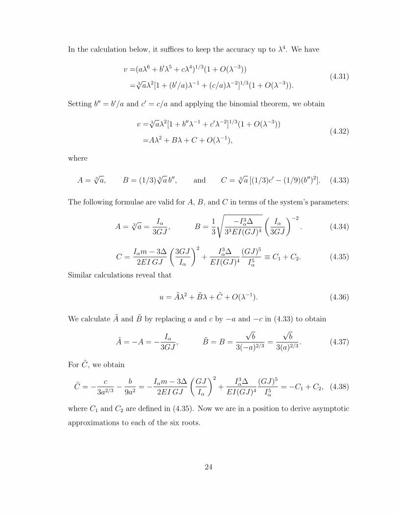
In the calculation below, it suffices to keep the accuracy up to λ4. We have

v =(aλ6 + b′λ5 + cλ4)1/3(1 + O(λ−3))

= 3√

aλ2[1 + (b′/a)λ−1 + (c/a)λ−2]1/3(1 + O(λ−3)).(4.31)

Setting b′′ = b′/a and c′ = c/a and applying the binomial theorem, we obtain

v = 3√

aλ2[1 + b′′λ−1 + c′λ−2]1/3(1 + O(λ−3))

=Aλ2 + Bλ + C + O(λ−1),(4.32)

where

A = 3√

a, B = (1/3) 3√

a b′′, and C = 3√

a [(1/3)c′ − (1/9)(b′′)2]. (4.33)

The following formulae are valid for A, B, and C in terms of the system’s parameters:

A = 3√

a =Iα

3GJ, B =

1

3

√−I3

α∆

33EI(GJ)4

(Iα

3GJ

)−2

. (4.34)

C =Iαm− 3∆

2EI GJ

(3GJ

Iα

)2

+I3α∆

EI(GJ)4

(GJ)5

I5α

≡ C1 + C2. (4.35)

Similar calculations reveal that

u = Aλ2 + Bλ + C + O(λ−1). (4.36)

We calculate A and B by replacing a and c by −a and −c in (4.33) to obtain

A = −A = − Iα

3GJ, B = B =

√b

3(−a)2/3=

√b

3(a)2/3. (4.37)

For C, we obtain

C = − c

3a2/3− b

9a2= −Iαm− 3∆

2EI GJ

(GJ

Iα

)2

+I3α∆

EI(GJ)4

(GJ)5

I5α

= −C1 + C2, (4.38)

where C1 and C2 are defined in (4.35). Now we are in a position to derive asymptotic

approximations to each of the six roots.

24

4.2 First Pair of Roots of the Characteristic Equation

We begin with the formula for x1 (see (4.15))

x1 =

√u− v −

(Iα

3GJ

)λ2. (4.39)

Substituting expressions for u and v from (4.13) and (4.14), and recalling that v is

the same with the appropriate sign changes yields

x1 =

3

√−

(Iα

3GJ

)3

λ6 − Iαm− 3∆

6EI GJλ4 +

√Q −

3

√(Iα

3GJ

)3

λ6 +Iαm− 3∆

6EI GJλ4 +

√Q− Iα

3GJλ2

1/2

,

(4.40)

where Q is given in (4.12). To calculate an asymptotic approximation for x1, we

substitute asymptotic approximations (4.32) and (4.36) into formula (4.39) to obtain

x1 =

√Aλ2 + Bλ + C − Aλ2 −Bλ− C − Iα

3GJλ2 + O(λ−1). (4.41)

where A, B, and C are given by formulae (4.34) and (4.35) and A, B, and C are

given in (4.37) and (4.38). The results of calculations from (4.35), (4.37) and (4.38)

allow us to write

x1 =

√−Aλ2 + Bλ− C1 + C2 − Aλ2 −Bλ− C1 − C2 − Iα

3GJλ2 + O(λ−1). (4.42)

Combining like terms yields

x1 =

√(−2A− Iα

3GJ

)λ2 − 2C1 (1 + O(λ−3)). (4.43)

We continue calculations to obtain an expression for x1 in the desired form (4.24).

Making the substitution A1 = −2A − Iα(3GJ)−1 and then factoring out the term

containing λ2 leads to the result

x1 = A1/21 λ

[1− 2C1

A1

λ−2

]1/2

(1 + O(λ−3)). (4.44)

25

Setting C2 = −2C1/A1 and using the binomial theorem, we obtain that

x1 = A1/21 λ

[1 +

1

2C2λ

−2 − 1

8C2

2λ−4 + O(λ−6)

] (1 + O(λ−3)

). (4.45)

Opening the brackets in (4.45) leads to the formula

x1 = A1/21 λ +

1

2A

1/21 C2λ

−1 + O(λ−2), (4.46)

which yields an expression for x1 in the desired form

x1 = A2λ + C3λ−1 + O(λ−2), (4.47)

where we have made the substitution A2 = A1/21 and C3 = 1

2A

1/21 . The asymptotic

expression of the second root can be given in the form

x2 = −x1 = −A2λ− C3λ−1 + O(λ−2). (4.48)

It remains to find expressions for A2 and C3 in terms of the parameters of the

system. We calculate A2 as

A2 = A1/21 =

(−2A− Iα

3GJ

)1/2

=

(−2

Iα

3GJ− Iα

3GJ

)1/2

= i

√Iα

GJ. (4.49)

We also calculate C3 as

C3 =1

2A

1/21 C2 = − C1

A1/21

. (4.50)

Using the substitution involving A1 and calculation (4.35) gives

C3 =−(Iαm− 3∆)

i(2EI GJ)

(GJ

Iα

)21(

2Iα

3GJ+

Iα

3GJ

)1/2=

i(Iαm− 3∆)

2EI GJ

(Iα

GJ

)2 (Iα

GJ

)1/2.

(4.51)

Finally substitution of ∆ = Iαm− S2 yields

C3 =i(Iαm− 3(Iαm− S2))

2EI GJ

(GJ

Iα

)5/2

=i(3S2 − 2Iαm)

2EI GJ

(GJ

Iα

)5/2

. (4.52)

Thus, we have obtained asymptotic expressions (4.46) and (4.48) for two roots

with the constants A2 and C3 being given in terms of the parameters of the system

in (4.49) and (4.52).

26

4.3 Second Pair of Roots of the Characteristic Equation

In this section we calculate asymptotic approximations to the roots x3 and x4

beginning with formulae (4.19) and (4.20). We start with the expression for x3

x3 =

√ei2π/3u− e−i2π/3v − Iα

3GJλ2. (4.53)

Using formulae (4.23), we rewrite (4.53) in the form

x3 =

√√√√(−1

2+ i

√3

2

)u +

(1

2+ i

√3

2

)v − Iα

3GJλ2. (4.54)

We separate the real and the imaginary parts in (4.54) to obtain

x3 =

√1

2(v − u) + i

√3

2(v + u)− Iα

3GJλ2. (4.55)

Using asymptotic formulae (4.32) and (4.36) for u and v, we calculate

v − u = Aλ2 + Bλ + C + O(λ−1)− Aλ2 − Bλ− C

= (A− (−A))λ2 + (B −B)λ + (C1 + C2)− (−C1 + C2) + O(λ−1)

= 2Aλ2 + 2C1 + O(λ−1).

(4.56)

To derive (4.56), we have used (4.35), (4.37), and (4.38). Similarly we calculate

v + u =(A + A)λ2 + (B + B)λ + C + C + O(λ−1)

=(A− A)λ2 + (B + B)λ + (C1 + C2) + (−C1 + C2) + O(λ−1)

=2Bλ + 2C2 + O(λ−1).

(4.57)

Now we notice that the leading term in the expression for (v − u) is quadratic with

respect to λ while the leading term in the expression for (v +u) is linear with respect

to λ. Substituting (4.56) and (4.57) into formula (4.55) for x3, we have

x3 =

√Aλ2 + C1 + O(λ−1) + i

√3(Bλ + C2 + O(λ−1))− Iα

3GJλ2. (4.58)

27

Combining terms having the same powers of λ and substituting the expression for A

from (4.34), we obtain

x3 =

√Iα

3GJλ2 − Iα

3GJλ2 + i

√3Bλ + (C1 + i

√3C2) + O(λ−1), (4.59)

which shows us that the terms containing λ2 cancel. Making the substitutions B3,1 =

i√

3B, C3,3 = C1 + i√

3C2, we can represent x3 as

x3 =√

B3,1λ + C3,3 + O(λ−1). (4.60)

Applying the binomial theorem to (4.60) and setting C3,4 = C3,3/B3,1 and B3,2 =

(B3,1)1/2, we modify the representation for x3 and have

x3 =[B3,1λ + C3,3]1/2(1 + O(λ−2))

=B1/23,1 λ1/2

[1 +

C3,3

B3,1

λ−1

]1/2

(1 + O(λ−2)

=B3,2λ1/2[1 + C3,4λ

−1]1/2(1 + O(λ−2)).

(4.61)

After application of the binomial theorem to the factor [1 + C3,4λ−1]1/2, we obtain

x3 = B3,2λ1/2

[1 +

1

2C3,4λ

−1 +1

8C2

3,4λ−2 + O(λ−3)

](1 + O(λ−2)). (4.62)

Making the substitution C3,5 = 12C3,4 and simplifying (4.62), we obtain

x3 = B3,2λ1/2 + B3,2C3,5λ

−1/2 + O(λ−3/2). (4.63)

Replacing B3,2C3,5 with C3,6, we obtain the desired asymptotic approximation for x3

x3 = B3,2λ1/2 + C3,6λ

−1/2 + O(λ−3/2). (4.64)

It remains to calculate expressions for B3,2 and C3,6 in terms of the parameters of

the system. For B3,2 we calculate by using formulae (4.34)

B3,2 = B1/23,1 = [i

√3B]1/2 = i

[ √3Iα

√Iα∆

3√

3(GJ)2√

EI· 32(GJ)2

3I2α

]1/2

= i

[∆

Iα EI

]1/4

, (4.65)

where ∆ is defined in (2.4). Using (4.65), we obtain for C3,6 the following expression:

28

C3,6 = B3,2C3,5 =1

2B

1/23,1 C3,4 =

1

2B

1/23,1

C3,3

B3,1

=C3,3

2B3,2

=C1 + i

√3C2

2B3,2

. (4.66)

Here we have recognized that we have calculate B1/23,1 as B3,2 in (4.65). We calculate

C1 and C2 separately. First we calculate C1 using appropriate substitutions starting

with results in calculation (4.35)

C1 =

(Iαm− 3∆

6EI GJ

) (1

3

)(3GJ

Iα

)2

=(Iαm− 3∆)(GJ)

2 EI I2α

. (4.67)

Similarly starting from (4.35) we have

C2 =

(I3α∆

33EI(GJ)4

)((3GJ)5

9I5α

)=

∆ GJ

EI I2α

. (4.68)

Having C1 and C2, we obtain for C3,6

C3,6 =

(Iαm− 3∆)(GJ)

2(EI)(Iα)2+ i√

3∆(GJ)

EI(Iα)2

−2i

[Iαm− S2

Iα EI

]1/4. (4.69)

Keeping in mind that x4 = −x3, we complete the approximations for the second pair

of roots of Eq. (3.27).

4.4 Third Pair of Roots of the Characteristic Equation

To calculate the approximations for the two remaining roots of Eq.(3.27), we will

use the same approach as in Section 4.3. Thus, we briefly outline the main steps of

the derivation. We recall that

x5 =

√ei4π/3u− e−i4π/3v − Iα

3GJλ2. (4.70)

Substituting (4.23) into (4.70) and separating real and imaginary parts under the

square root, we have

x5 =

√1

2(v − u)− i

√3

2(v + u)− Iα

3GJλ2. (4.71)

29

Substituting asymptotic formulae (4.56) and (4.57) for (v−u) and (v+u) respectively

and collecting like terms, we obtain

x5 =

√−i√

3Bλ + C1 − i√

3C2 + O(λ−1). (4.72)

It can be easily seen that

x5 =

√−i√

3Bλ + C1 − i√

3C2 (1 + O(λ−2)). (4.73)

Next we substitute B5,1 = −i√

3B and C5,3 = C1 − i√

3C2 to have

x5 =√

B5,1λ + C5,3 (1 + O(λ−2)) = B1/25,1 λ1/2

[1 +

C5,3

B5,1

λ−1

]1/2

(1 + O(λ−2)). (4.74)

Setting B5,2 = B1/25,1 and C5,4 = C5,3/B5,1 and then using the binomial theorem, we

have

x5 =B5,2λ1/2[1 + 1/2C5,4λ

−1 + O(λ−2)](1 + O(λ−2)

=B5,2λ1/2 + 1/2B5,2C5,4λ

−1/2 + O(λ−3/2).(4.75)

Finally, we arrive at the desired expression for x5, i.e.,

x5 = B5,2λ1/2 + C5,5λ

−1/2 + O(λ−3/2), (4.76)

where C5,5 stands for 1/2B5,2C5,4.

To conclude this section, we derive formulae for the coefficients in terms of the

problem’s structural parameters. Using formulae (4.34), we have

B5,2 = B1/25,1 = [−i

√3B]1/2 =

[ √3Iα

√Iα∆

3√

3(GJ)2√

EI· 32(GJ)2

3I2α

]1/2

=

[∆

Iα EI

]1/4

, (4.77)

Using formulae (4.67) and (4.68), we calculate C5,5

C5,5 =1

2(−i

√3B)1/2 C5,3

B5,1

=1

2

−i(√

3B)1/2(C1 − i√

3C2)

−i√

3B

=1

2

(C1 − i√

3C2)

(−i√

3B)1/2=

(Iαm− 3∆)(GJ)

2(EI)(Iα)2− i√

3∆(GJ)

EI(Iα)2

2

[Iαm− S2

Iα EI

]1/4.

(4.78)

Since x6 = −x5, we have the approximation for x6 as well.

30

4.5 General Solution to the Spectral Equation for the

Operator Pencil

In this section, we bring the results of the last three sections together in order to

write the general solution of the differential equation P(λ)φ = 0. We recall that in

Sections 4.2–4.4, we have calculated the approximations to the roots of the charac-

teristic equation (3.27). For convenience, we reproduce those results below.

x1,2 = ±i

√Iα

GJλ + C3λ

−1 + O(λ−2), (4.79)

x3,4 = ±i

[∆

Iα EI

]1/4

λ1/2 + C3,6λ−1/2 + O(λ−3/2), (4.80)

x5,6 = ±[

∆

Iα EI

]1/4

λ1/2 + C5,6λ−1/2 + O(λ−3/2), (4.81)

with C3, C3,6, and C5,5 begin defined in (4.52)), (4.69) and (4.78).

The general solution to the sixth order ordinary differential equation can be repre-

sented as a linear combination of exponential–like functions. To simplify subsequent

calculations, we introduce the notation

x1,2 = ±iΓ(λ), x3,4 = ±iγ(λ), x5,6 = ±γ(λ), (4.82)

where Γ, γ, and γ are defined by the following formulae:

γ(λ) = Pλ1/2 + O(λ−1/2) = Pλ1/2(1 + O(λ−1)), (4.83)

γ(λ) = Pλ1/2 + O(λ−1/2) = Pλ1/2(1 + O(λ−1)), (4.84)

Γ(λ) = Qλ + O(λ−1) = Qλ(1 + O(λ−2)), (4.85)

where P =

[∆

IαEI

]1/4

, Q = R1/2 =

[Iα

GJ

]1/2

. (4.86)

Using notations (4.83)–(4.86), we may write the general solution Ψ of the equation

P(λ)φ = 0 in the following form:

Ψ(λ, x) =A(λ)eγ(λ)(x+L) + B(λ)eiγ(λ)(x+L) + C(λ)eiΓ(λ)(x+L)+

D(λ)e−γ(λ)(x+L) + E(λ)e−iγ(λ)(x+L) + F(λ)e−iΓ(λ)(x+L),(4.87)

with A(·), B(·), C(·), D(·), E(·), and F(·) being arbitrary functions of λ.

31

CHAPTER V

The Left–Reflection Matrix

5.1 Two–step Procedure for Applying Boundary Conditions

As stated in Section 3.2, our ultimate goal is to find such values of the complex

parameter λ, for which the equation LΨ = λΦ has nontrivial solutions, i.e., to find the

eigenvalues and eigenvectors of the operator L. We have shown that the aforemen-

tioned problem is equivalent to the problem of finding eigenvalues and eigenfunctions

of the pencil P(·), i.e., to the problem of finding the values of λ for which the equation

P(λ)φ = 0 has nontrivial solutions. This is exactly the problem we will focus on in

Chapters V–VII. Thus, we are looking for a solution of the equation

P(λ)Ψ = 0, (5.1)

which can be represented in the form (4.87). More precisely, we are looking for those

λ ∈ C, for which there exist coefficients A(λ), B(λ), C(λ), D(λ),E(λ), and B(λ), such

that Ψ(x, λ) satisfies the boundary conditions given in (3.26).

Substituting Ψ into these boundary conditions gives us a linear system of six equa-

tions in six unknowns A(·), B(·), C(·), D(·), E(·), and F(·). LetM be the 6×6 matrix

of coefficients from the aforementioned system. Since our system is homogeneous, it

can be written as MZ = 0, where ZT (λ) = {A(λ),B(λ), C(λ),D(λ), E(λ),F(λ)}.Thus, we have to find approximations for the solutions of the equation detM(λ) = 0.

It turns out that directly finding approximations for the roots of this determinant is

an extremely difficult problem. So, we suggest an alternative approach. Namely, let

us introduce two 3–component vectors

X(λ) = (A(λ),B(λ), C(λ))T , Y (λ) = (D(λ), E(λ),F(λ))T , (5.2)

and first select only three boundary conditions, the conditions which have to be

imposed on the solution Ψ to satisfy the boundary conditions at the left end of the

32

beam. As a result, we obtain the relation between the vectors X(·) and Y (·), which

can be written in the form

X(λ) = Rl(λ)Y (λ). (5.3)

A corresponding 3 × 3 matrix Rl(·) in (5.3) we call the left–reflection matrix.

Therefore, if the vectors X(·) and Y (·) are connected through the left–reflection

matrix, the corresponding function (4.87) satisfies equation (5.1) and the left end

boundary conditions. Secondly, let us select only the right–end boundary conditions.

We obtain from three right end boundary conditions, that the following relation

between X(·) and Y (·) holds:

X(λ) = Rr(λ)Y (λ), (5.4)

where the 3 × 3 matrix Rr(·) we call the right–reflection matrix. So, if the vectors

X(·) and Y (·) are connected through relation (5.4), the corresponding function (4.87)

satisfies equation (5.1) and three boundary conditions at the right end.

It can be easily verified that to satisfy all six boundary conditions, the following

equation must be valid:

A(λ)

B(λ)

C(λ)

D(λ)

E(λ)

F(λ)

=

0 Rr(λ)

R−1l (λ) 0

A(λ)

B(λ)

C(λ)

D(λ)

E(λ)

F(λ)

. (5.5)

Eq.(5.5) is certainly equivalent to the following one:

33

I−

0 Rr

R−1l 0

A(λ)

B(λ)

C(λ)

D(λ)

E(λ)

F(λ)

= 0, (5.6)

where I is the identity matrix. We notice that a solution of Eq.(5.6) is nontrivial if

and only if

det

I−

0 Rr(λ)

R−1l (λ) 0,

= 0, (5.7)

or equivalently

det(I− R−1l (λ)Rr(λ)) = 0. (5.8)

We may factor out R−1l and obtain

det(R−1l (λ)) det(Rl(λ)− Rr(λ)) = 0, (5.9)

so that since R−1l exists (as will be shown later), we obtain

det(Rl(λ)− Rr(λ)) = 0. (5.10)

Thus we have reduced the problem involving a 6× 6 matrix to a similar problem

for a 3× 3 matrix. From now on, we will carry out the following steps:

• calculate the left and right–reflection matrices;

• find approximations for the roots of Eq.(5.10).

5.2 Left–Reflection Matrix

In this section, we will derive an asymptotic approximation for the left–reflection

matrix Rl. Let us substitute the general solution Ψ(·) given in (4.87) into each of

34

the three left–hand boundary conditions of the operator pencil. Substituting into the

first one gives us the first equation for unknown coefficients

A(λ) + B(λ) + C(λ) +D(λ) + E(λ) + F(λ) = 0. (5.11)

Substituting Ψ(·) from (4.87) into the second one gives us the second equation

A(λ)γ(λ)+B(λ)iγ(λ)+ C(λ)iΓ(λ)−D(λ)γ(λ)−E(λ)iγ(λ)−F(λ)iΓ(λ) = 0. (5.12)

with γ(·), γ(·), and Γ(·) being defined in (4.83)–(4.85). And lastly substituting Ψ(·)into the third boundary condition (3.20) yields

[A(λ)γ4(λ) +B(λ)γ4(λ) + C(λ)Γ4(λ) +D(λ)γ4(λ) + E(λ)γ4(λ) +F(λ)Γ4(λ)] + 0 = 0.

(5.13)

Rearranging the above three equations so that the functions A(·), B(·), and C(·) are

on one side while the functions D(·), E(·), and F(·) are on the other side results in

the following linear system of three equations:

A(λ) + B(λ) + C(λ) = −D(λ)− E(λ)−F(λ), (5.14)

γ(λ)A(λ) + iγ(λ)B(λ) + iΓ(λ)C(λ) = γ(λ)D(λ) + iγ(λ)E(λ) + iΓ(λ)F(λ), (5.15)

γ4(λ)A(λ)+ γ4(λ)B(λ)+Γ4(λ)C(λ) = −γ4(λ)D(λ)− γ4(λ)E(λ)−Γ4(λ)F(λ). (5.16)

Clearly, the three equation (5.14)–(5.16) can be written as one matrix equation

1 1 1

γ(λ) iγ(λ) iΓ(λ)

γ4(λ) γ4(λ) Γ4(λ)

A(λ)

B(λ)

C(λ)

=

−1 −1 −1

γ(λ) iγ(λ) iΓ(λ)

−γ4(λ) −γ4(λ) −Γ4(λ)

D(λ)

E(λ)

F(λ)

. (5.17)

Thus we have a matrix equation in the form

A(λ)X(λ) = B(λ)Y (λ), (5.18)

35

where the vectors X(·) and Y (·) are defined in (5.2). If we solve Eq.(5.18) for X(·)

X(λ) = A−1(λ)B(λ)Y (λ), (5.19)

then we observe that the left–reflection matrix as described in (5.3) can be given as

Rl(λ) = A−1(λ)B(λ). (5.20)

While the straightforward calculation of the above left–reflection matrix is possi-

ble, we exploit the similarity of the entries of A and B to make the calculation easier.

We notice that

B(λ) = −A(λ) + V(λ), (5.21)

where

V(λ) = 2

0 0 0

γ(λ) iγ(λ) iΓ(λ)

0 0 0

. (5.22)

Thus the calculation of Rl(·) can be simplified, for using this expression for B(·) in

terms of A(·) we have that

Rl(λ) = A−1(λ)B(λ) = A−1(λ)(−A(λ) + V(λ)) = −I+ A−1(λ)V(λ). (5.23)

This alternate expression for Rl(·) will make its calculation easier because only the

middle column of A−1(·) is needed for the calculation of A−1(·)V(·) since V(·) has

only one non–zero row. So recalling that

A(λ) =

1 1 1

γ(λ) iγ(λ) iΓ(λ)

γ4(λ) γ4(λ) Γ4(λ)

, (5.24)

36

we calculate asymptotic approximations to the middle column of A−1(·) using Cramer’s

Rule. First we calculate detA by expansion with respect to the bottom row entries

(detA)(λ) = γ4(λ)

∣∣∣∣∣∣1 1

iγ(λ) iΓ(λ)

∣∣∣∣∣∣− γ4(λ)

∣∣∣∣∣∣1 1

iγ(λ) iΓ(λ)

∣∣∣∣∣∣+ Γ4(λ)

∣∣∣∣∣∣1 1

γ(λ) iγ(λ)

∣∣∣∣∣∣.

(5.25)

Substituting expressions (4.83)–(4.85) into (5.25), we find that the terms containing

γ4 and γ4 behave as O(λ3) when |λ| → ∞, while the term containing Γ4 behaves as

O(λ4.5) when |λ| → ∞. The latter fact means that we can proceed as follows:

(detA)(λ) = Γ4(λ)(iγ(λ)−γ(λ))+O(λ3) = Γ4(λ)(iγ(λ)−γ(λ))(1+O(λ−1.5)). (5.26)

Substituting formulae (4.83) and (4,84) into (5.26) leads to

(detA)(λ) = Γ4(λ)[Pλ1/2(i− 1) + O(λ−1/2)](1 + O(λ−1.5))

= Γ4(λ)[Pλ1/2(i− 1)](1 + O(λ−1)).(5.27)

Now we proceed to find each specific entry of the middle column of the matrix

A−1(·) given by (5.24). Let C2j, j = 1, 2, 3, be a cofactor corresponding to the second

row, and the j–th entry of A(·). Beginning with the first entry of A−1(·), we have

A−112 (λ) =

C21

(detA)(λ)=

−1

(detA)(λ)

∣∣∣∣∣∣1 1

γ4(λ) Γ4(λ)

∣∣∣∣∣∣=

−(Γ4(λ)− γ4(λ))

Γ4(λ)[Pλ1/2(i− 1)](1 + O(λ−1/2).

(5.28)

Recalling that Γ(·) behaves as O(λ) while γ(·) behaves as O(λ1/2), we may rewrite

the numerator so that

A−112 (λ) =

−Γ4(λ)(1 + O(λ−2))

Γ4(λ)[Pλ1/2(i− 1) + O(λ−1/2)]=

1 + O(λ−2)

(1− i)Pλ1/2(1 + O(λ−1)). (5.29)

Now using the fact that

1

1 + O(λm)= 1 + O(λm) + O(λ2m) + . . . = 1 + O(λm), m < 0, (5.30)

we can finally write

A−112 (λ) =

1

(1− i)P−1λ−1/2(1 + O(λ−1)). (5.31)

37

Thus we have obtained an asymptotic expression of A−112 . In what follows, it is con-

venient to use the notation

ωij(λ) = 1 + O(λ−1), (5.32)

which means that on the intersection of the i− th row and the j − th column, there

is a factor 1 + O(λ−1). Thus we may finally write that

A−112 =

1 + i

2P−1λ−1/2ω12. (5.33)

Calculations of the other two needed entries of A−1(·) will proceed in a similar manner.

Calculating A−122 (·), we have

A−122 (λ) =

C22

(detA)(λ)=

(−1)4

Γ4(λ)[Pλ1/2(i− 1)]ω22(λ)

∣∣∣∣∣∣1 1

γ4(λ) Γ4(λ)

∣∣∣∣∣∣

=Γ4(λ)− γ4(λ)

Γ4(λ)[Pλ1/2(i− 1)]ω22(λ).

(5.34)

Substituting expressions (4.83) into the numerator we find that γ4(·) behaves as

O(λ2). Thus we may rewrite the numerator and have

A−122 (λ) = −i + 1

2P−1λ−1/2ω22(λ). (5.35)

Calculating the remaining entry, we have

A−132 (λ) =

C23

(detA)(λ)=

−1

Γ4(λ)[Pλ1/2(i− 1)](1 + O(λ−1))

∣∣∣∣∣∣1 1

γ4(λ) γ4(λ)

∣∣∣∣∣∣

=γ4(λ)− γ4(λ)

Γ4(λ)[Pλ1/2(i− 1)](1 + O(λ−1)).

(5.36)

Using formulae (4.83) and (4.84), we can see that γ4(λ) − γ4(λ) = O(λ). Substi-

tuting the expression for Γ(·) from (4.85) and simplifying, we obtain

A−132 (λ) =

O(λ)

P λ4(1 + O(λ−2))[Pλ1/2(i− 1)](1 + O(λ−1))= O(λ−3.5). (5.37)

Using formula (5.22) for V and (5.23) for Rl, we obtain

38

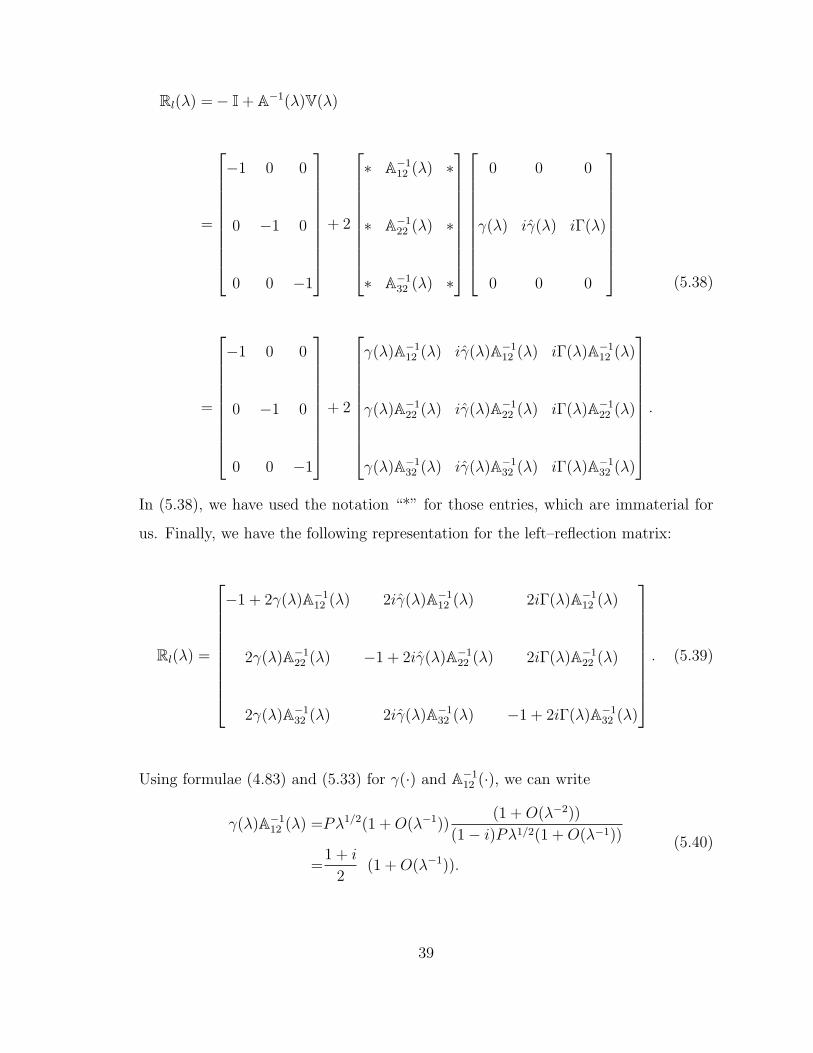
Rl(λ) =− I+ A−1(λ)V(λ)

=

−1 0 0

0 −1 0

0 0 −1

+ 2

∗ A−112 (λ) ∗

∗ A−122 (λ) ∗

∗ A−132 (λ) ∗

0 0 0

γ(λ) iγ(λ) iΓ(λ)

0 0 0

=

−1 0 0

0 −1 0

0 0 −1

+ 2

γ(λ)A−112 (λ) iγ(λ)A−1

12 (λ) iΓ(λ)A−112 (λ)

γ(λ)A−122 (λ) iγ(λ)A−1

22 (λ) iΓ(λ)A−122 (λ)

γ(λ)A−132 (λ) iγ(λ)A−1

32 (λ) iΓ(λ)A−132 (λ)

.

(5.38)

In (5.38), we have used the notation “*” for those entries, which are immaterial for

us. Finally, we have the following representation for the left–reflection matrix:

Rl(λ) =

−1 + 2γ(λ)A−112 (λ) 2iγ(λ)A−1

12 (λ) 2iΓ(λ)A−112 (λ)

2γ(λ)A−122 (λ) −1 + 2iγ(λ)A−1

22 (λ) 2iΓ(λ)A−122 (λ)

2γ(λ)A−132 (λ) 2iγ(λ)A−1

32 (λ) −1 + 2iΓ(λ)A−132 (λ)

. (5.39)

Using formulae (4.83) and (5.33) for γ(·) and A−112 (·), we can write

γ(λ)A−112 (λ) =Pλ1/2(1 + O(λ−1))

(1 + O(λ−2))

(1− i)Pλ1/2(1 + O(λ−1))

=1 + i

2(1 + O(λ−1)).

(5.40)

39

A similar calculation for γ(·)A−112 (·) yields

γ(λ)A−112 (λ) =Pλ1/2(1 + O(λ−1/2))

(1 + O(λ−2))

(1− i)Pλ1/2(1 + O(λ−1))

=1 + i

2(1 + O(λ−1)).

(5.41)

Using (4.85) and (5.33), we calculate Γ(·)A−112 (·) and have

Γ(λ)A−112 (λ) =

√Iα/GJλ(1 + O(λ−2))

(1 + O(λ−2))

(1− i)Pλ1/2(1 + O(λ−1))

=

√Iα

GJP−1λ1/2 (i + 1)

2(1 + O(λ−1)).

(5.42)

Now we move on to the second row of the matrix Rl. Using (4.84) and (5.35), we

calculate that

γ(λ)A−122 (λ) = −Pλ1/2 (i + 1)

2P−1λ−1/2ω22 = −(i + 1)ω22

2. (5.43)

Thus we substitute this expression into the entire expression for (Rl)22 in (5.39) and

simplify to have

(Rl)22 (λ) = −1 + 2A−122 (λ)iγ(λ) = −1− i(i + 1)ω22(λ) = −iω22(λ). (5.44)

Now considering the entry (Rl)21, we substitute (4.84) and (5.35) and have

(Rl)21 (λ) = 2γ(λ)A−122 (λ) = −[Pλ1/2ω22(λ)](i + 1)P−1λ−1/2ω22(λ) = −(i + 1)ω22(λ).

(5.45)

Turning now to (Rl)23 (·), we calculate a part of it by substitution (4.85) and (5.35)

Γ(λ)A−122 (λ) =

[√Iα

GJλ(1 + O(λ−2))

][−(i + 1)

2P−1λ−1/2ω22(λ)

]

=− (i + 1)

2

√Iα

GJP−1λ1/2ω22(λ).

(5.46)

Thus we may calculate the entry (Rl)23 (·) as

(Rl)23 (λ) = 2iΓ(λ)A−122 (λ) = (1− i)

√Iα

GJP−1λ1/2ω23(λ). (5.47)

40

Finally we evaluate the third row of Rl(·). We calculate a portion of the first entry

using (4.83) as well as (5.36) to find that

γ(λ)A−132 (λ) = Pλ1/2(1 + O(λ−1))O(λ−3.5) = O(λ−3). (5.48)

Similarly, we calculate a portion of the second entry as

γ(λ)A−132 (λ) = Pλ1/2(1 + O(λ−1))O(λ−3.5) = O(λ−3). (5.49)

And finally we calculate a portion of the last entry as

Γ(λ)A−132 (λ) =

√Iα

GJλ(1 + O(λ−2))O(λ−3.5) = O(λ−2.5). (5.50)

Substituting the results of (5.40)–(5.42), (5.44)–(5.46), and (5.48)–(5.50) into

(5.39) for Rl(·) and simplifying, we obtain the following asymptotic approximation to

the left–reflection matrix:

Rl(λ) =

iω11(λ) (i− 1)ω12(λ)

√Iα

GJP−1(i− 1)λ1/2ω13(λ)

−(i + 1)ω21(λ) −iω22(λ)

√Iα

GJP−1(1− i)λ1/2ω23(λ)

O(λ−3) O(λ−3) −1 + O(λ−2.5)

. (5.51)

41

CHAPTER VI

Right–Reflection Matrix

Now we will look for the right–reflection matrix Rr by substituting the general

solution Ψ(·) from (4.87) into the right end boundary conditions (3.21) and (3.24).

In what follows, it is convenient to introduce new notation

exp{γ(λ)L} ≡ e(λ) ≡ eγ(λ)L,

exp{iγ(λ)L} ≡ e(λ) ≡ eiγ(λ)L,

exp{iΓ(λ)L} ≡ e+(λ) ≡ eiΓ(λ)L.

(6.1)

We also recall that by (4.86)

P =

[∆

Iα EI

]1/4

, R1/2 = Q =

[Iα

GJ

]1/2

. (6.2)

Beginning with the first right end boundary condition Ψ′′′(0) = 0 (as stated in

(2.15)), we substitute Ψ(·) from (4.87) and use definition (6.1) to obtain

γ3(λ)A(λ)e(λ)− iγ3(λ)B(λ)e(λ)− iΓ3(λ)C(λ)e+(λ)−γ3(λ)D(λ)e(λ)−1 + iγ3(λ)E(λ)e(λ)−1 + iΓ3(λ)F(λ)e+(λ)−1 = 0.

(6.3)

To proceed, we need the following estimates:

γ(λ)

γ(λ)= (1 + O(λ−1)),

Γ(λ)

γ(λ)=

Q

Pλ1/2 (1 + O(λ−1)). (6.4)

Thus after dividing (6.3) by γ3(λ) and substituting (6.4) into the result, we obtain

A(λ)e(λ)− i(1 + O(λ−1))B(λ)e(λ)− iQ3

P 3λ3/2(1 + O(λ−1))C(λ)e+(λ)

−D(λ)e(λ)−1 + i(1 + O(λ−1))E(λ)e(λ)−1 + iQ3

P 3λ3/2(1 + O(λ−1))F(λ)e+(λ)−1 = 0.

(6.5)

Let us leave the terms containing A(·), B(·) and C(·) on the left side of equation (6.5)

while moving the terms with D(·), E(·), and F(·) to the right side to obtain

A(λ)e(λ)− i(1 + O(λ−1))B(λ)e(λ)− iQ3

P 3λ3/2(1 + O(λ−1))C(λ)e+(λ) =

D(λ)e(λ)−1 − i(1 + O(λ−1))E(λ)e(λ)−1 − iQ3

P 3λ3/2(1 + O(λ−1))F(λ)e+(λ)−1.

(6.6)

42

Now we turn to the second right–hand side boundary condition of the operator pencil

given in (3.21) as

EIϕ′′0(0) + ghiλϕ′0(0) = 0. (6.7)

Substituting in Ψ(·) from (4.87) and using notation (6.1), we obtain

EI[γ2(λ)A(λ)e(λ)− γ2(λ)B(λ)e(λ)− Γ2(λ)C(λ)e+(λ) + γ2(λ)D(λ)e(λ)−1−γ2(λ)E(λ)e(λ)−1 − Γ2(λ)F(λ)e+(λ)−1] + ghiλ[γ(λ)A(λ)e(λ) + iγ(λ)B(λ)e(λ)+

iΓ(λ)C(λ)e+(λ)− γ(λ)D(λ)e(λ)−1 − iγ(λ)E(λ)e(λ)−1 − iΓ(λ)F(λ)e+(λ)−1] = 0.

(6.8)

For the next step, we need the following approximations:

1

γ(λ)= P−1λ−1/2(1 + O(λ−1)),

γ(λ)

γ2(λ)= P−1λ−1/2(1 + O(λ−1)),

Γ(λ)

γ2(λ)= QP−2(1 + O(λ−1)).

(6.9)

We divide (6.8) by γ2(·) using approximations (6.4) and (6.9), and then collect to-

gether terms involving each of A(·), B(·), C(·), D(·), E(·) and F(·) respectively. Let

Q1 be the coefficient for A(·). Q1 has the following asymptotic approximation:

Q1 ≡ [EI + ghiλP−1λ−1/2(1 + O(λ−1))]e(λ) = [EI + ghP−1iλ1/2](1 + O(λ−1))e(λ).

(6.10)

The coefficient for B(·), denoted by Q2, has the following asymptotic approximation:

Q2 ≡ −[EI

(γ(λ)

γ(λ)

)2

+ ghλγ(λ)

γ2(λ)

]e(λ) = [−EI − ghP

−1λ1/2](1 + O(λ−1))e(λ).

(6.11)

The coefficient Q3 before C(·) can be approximated as

Q3 ≡−[EI

(Γ(λ)

γ(λ)

)2

+ ghλΓ(λ)

γ2(λ)

]e+(λ)

=[−EIQ2P−2λ− ghλQP−2](1 + O(λ−1))e+(λ).

(6.12)

The coefficient Q4 before D(·) can be approximated as

Q4 ≡[EI − ghiλ

γ(λ)

γ2(λ)

]e(λ)−1 = [EI − ghP

−1iλ1/2](1 + O(λ−1))e(λ)−1. (6.13)

43

The coefficient Q5 before E(·) can be approximated as

Q5 ≡[−EI(

γ(λ)

γ(λ))2 + ghλ

γ(λ)

γ2(λ)

]e(λ)−1 = [−EI + ghP

−1λ1/2](1 + O(λ−1))e(λ)−1.

(6.14)

The coefficient Q6 before F(·) can be approximated as

Q6 ≡[−EI(

Γ(λ)

γ(λ))2 + ghλ

Γ(λ)

γ2(λ)

]e+(λ)−1

=[−EIQ2P−2λ + ghλQP−2](1 + O(λ−1))e+(λ)−1.

(6.15)

Thus we can write the second right–hand boundary condition by summing the results

of (6.10)–(6.15) and setting the sum equal to zero. Again we leave the terms involving

A(·), B(·) and D(·) on the left side and take the other terms to the right side to rewrite

Eq.(6.8) in the form

Q1A(λ) + Q2B(λ) + Q3 C(λ) = − [Q4D(λ) + Q5 E(λ) + Q6F(λ)] .

The latter equation has the following asymptotic approximation:[EI + gh

1

Piλ1/2

](1 + O(λ−1))A(λ)e(λ) +

[−EI − gh

1

Pλ1/2

]×

(1 + O(λ−1))B(λ)e(λ)−[EI

Q2

P 2λ + ghλ

Q

P 2

](1 + O(λ−1))C(λ)e+(λ) =

[−EI + gh

1

Piλ1/2

](1 + O(λ−1))D(λ)e(λ)−1 +

[EI − gh

1

Pλ1/2

]×

(1 + O(λ−1))E(λ)e(λ)−1 +

[EI

Q2

P 2λ− ghλ

Q

P 2

](1 + O(λ−1))F(λ)e+(λ)−1.

(6.16)

Examining the third right–hand boundary condition given in (3.24), we realize

that we need the function Ψ(·), along with its first, fourth, and fifth derivatives

evaluated at zero. So using Ψ(·) from (4.87) and definition (6.1) yields

Ψ(λ, 0) = A(λ)e(λ)+B(λ)e(λ)+C(λ)e+(λ)+D(λ)e(λ)−1+E(λ)e(λ)−1+F(λ)e+(λ)−1.

(6.17)

The first derivative of the general solution evaluated at x = 0 is

Ψ′(λ, 0) = γ(λ)A(λ)e(λ) + iγ(λ)B(λ)e(λ) + iΓ(λ)C(λ)e+(λ)−γ(λ)D(λ)e(λ)−1 − iγ(λ)E(λ)e(λ)−1 − iΓ(λ)F(λ)e+(λ)−1.

(6.18)

44

The fourth derivative of the function Ψ(·) evaluated at x = 0 is

Ψ′′′′

(λ, 0) = γ4(λ)A(λ)e(λ) + γ4(λ)B(λ)e(λ) + Γ4(λ)C(λ)e+(λ)+

γ4(λ)D(λ)e(λ)−1 + γ4(λ)E(λ)e(λ)−1 + Γ4(λ)F(λ)e+(λ)−1.(6.19)

And the fifth derivative of the function Ψ(·) evaluated at x = 0 is

ΨV (λ, 0) = γ5(λ)A(λ)e(λ) + iγ5(λ)B(λ)e(λ) + iΓ5(λ)C(λ)e+(λ)−γ5(λ)D(λ)e(λ)−1 − iγ5(λ)E(λ)e(λ)−1 − iΓ5(λ)F(λ)e+(λ)−1.

(6.20)

After substituting results (6.18)–(6.20) into the sixth boundary condition (3.24), we

divide the resulting equation by γ2(·). The following approximations are valid:

γ4(λ)

γ2(λ)= P 2λ(1 + O(λ−1)),

1

γ2(λ)=

1

P 2λ−1(1 + O(λ−1)),

Γ5(λ)

γ2(λ)=

Q5

P 2λ4(1 + O(λ−1)),

Γ4(λ)

γ2(λ)=

Q4

P 2λ3(1 + O(λ−1)),

(6.21)

where P and Q are defined in (4.86). Now we substitute (6.17)–(6.20) into the third

right–hand boundary condition (3.24) leaving the terms involving A(·), B(·) and C(·)on the left side, and moving the terms involving D(·), E(·) and F(·) to the right side.

Let us collect together all the terms involving A(·)e(·) and denote the coefficient

for A(·)e(·) by A31. For A31, we have

A31(λ) = EI GJγ3(λ) + iEI gαλγ2(λ)−mGJ λ2 − igαmλ3γ−2(λ)

=

[EI GJP 3λ3/2 + iEI gαP 2λ2 −mGJ

1

Pλ3/2 − igαm

1

P 2λ2

](1 + O(λ−1/2))

= i

[EI gαP 2 − gαm

1

P 2

]λ2(1 + O(λ−1/2)).

(6.22)

Let us collect together all terms involving D(·)e(·)−1 and denote them by B31. For

B31, we have

B31(λ) = EI GJγ3(λ)− iEI gαλγ2(λ)−mGJ λ2 + igαmλ3γ−2(λ)

= i

[−EI gαP 2 + gαm

1

P 2

]λ2(1 + O(λ−1/2)).

(6.23)

45

Let us collect together all the terms involving B(·)e(·) and denote them by A32. For

A32, we have

A32(λ) = iEI GJγ5(λ)γ−2(λ) + iEI gαλγ4(λ)γ−2(λ)− imGJ λ2γ(λ)γ−2(λ)

− igαmλ3γ−2(λ) =

[iEI gαλP 2λ− igαmλ3 1

P 2λ−1

](1 + O(λ−1/2))

= i

[EI gαP 2 − gαm

1

P 2

]λ2(1 + O(λ−1/2)).

(6.24)

Let us collect together all the terms involving E(·)e(·)−1 and denote them by B32. For

B32, we have

B32(λ) =iEI GJγ5(λ)γ−2(λ)− iEI gαλγ4(λ)γ−2(λ)− imGJ λ2γ(λ)γ−2(λ)

+ igαmλ3γ−2(λ) =

[−iEI gαλP 2λ + igαmλ3 1

P 2λ−1

](1 + O(λ−1/2))

=i

[−EI gαP 2 + gαm

1

P 2

]λ2(1 + O(λ−1/2)).

(6.25)

Let us collect together all the terms involving C(·)e+(·) and denote them by A33. For

A33, we have

A33(λ) = iEI GJΓ5(λ)γ−2(λ) + iEI gαλΓ4(λ)γ−2(λ)− imGJ λ2Γ(λ)γ−2(λ)

− igαmλ3γ−2(λ) = iEI GJQ5

P 2λ4(1 + O(λ−1)) + iEI gαλ

Q4

P 2λ3(1 + O(λ−1))

= i

[EI GJ

Q5

P 2+ EIgα

Q4

P 2

]λ4(1 + O(λ−1)).

(6.26)

Let us collect together all the terms involving F(·)e+(·)−1 and denote them by B33.

For B33, we have

B33(λ) = iEI GJΓ5(λ)γ−2(λ)− iEI gαλΓ4(λ)γ−2(λ)− imGJ λ2Γ(λ)γ−2(λ)

+ igαmλ3γ−2(λ) = iEI GJQ5

P 2λ4(1 + O(λ−1))− iEI gαλ

Q4

P 2λ3(1 + O(λ−1))

= i

[EI GJ

Q5

P 2− EIgα

Q4

P 2

]λ4(1 + O(λ−1)).

(6.27)

46

Thus, we can write the third boundary condition (3.24) in the form

A31(λ)A(λ)e(λ) + A32(λ)B(λ)e(λ) + A33(λ)C(λ)e+(λ) =

B31(λ)D(λ)e(λ)−1 + B32(λ)E(λ)e(λ)−1 + B33(λ)F(λ)e+(λ)−1,(6.28)

where the coefficients Aij, Bij, i = 3, j = 1, 2, 3, are given by formulae (6.22)–(6.27).

Setting

E(λ) = diag(e(λ), e(λ), e+(λ)), (6.29)

we can write the three right–hand boundary conditions in the matrix form. This

matrix form, which will appear below, contains two matrices denoted by A(·) and

B(·). They are similar to the ones appearing in formula (5.18). Without any misun-

derstanding, we will use the notation keeping in mind that the new matrices A(·) and

B(·) are different from the ones which appeared in Section 5.2. Thus, we have

A(λ)E(λ) X(λ) = B(λ)E−1(λ) Y (λ), (6.30)

where the entries of the matrices of A(·) and B(·) are given in (6.6), (6.16), and

(6.22)–(6.28).

To rewrite the matrix equation (6.30) explicitly, it is convenient to introduce the

following notation: ωij(λ) and ωij(λ); ωij(λ), with i, j = 1, 2, 3, means that there is a

factor (1 + O(λ−1/2)) on the intersection of the i-th row and the j-th column in the

matrix below, and ωij(λ), with i, j = 1, 2, 3, means that there is a factor (1+O(λ−1))

on the intersection of the i-th row and the j-th column in the matrix below. With

the aforementioned notation, the matrix equation (6.30) then becomes

47

1 −iω12(λ) iQ3

P 3 λ3/2ω13(λ)

Q1(λ)e(λ)−1 Q2(λ)e(λ)−1 Q3(λ)e+(λ)−1

A31(λ) A32(λ) A33(λ)

E(λ)X(λ) =

1 −iω12(λ) −iQ3

P 3 λ3/2ω13(λ)

−Q4(λ)e(λ) −Q5(λ)e(λ) −Q6(λ)e+(λ)

−B31(λ) −B32(λ) −B33(λ)

E

−1(λ)Y (λ),

(6.31)

where Q1, Q2, Q3, Q4, Q5, and Q6 are defined by formulae (6.10)–(6.15); the entries

A3i(λ), i = 1, 2, 3, are defined by formulae (6.22), (6.24), and (6.26); the entries

B3i(λ), i = 1, 2, 3, are defined by formulae (6.23), (6.25), and (6.27) respectively.

Assuming that the matrix A−1(·) exists, we solve (6.30) for X(·) and obtain

X(λ) = E−1(λ)A−1(λ)B(λ)E−1(λ)Y (λ). (6.32)

Comparing (5.1) with (6.32), we conclude that the right–reflection matrix can be

represented as

Rr(λ) = E−1(λ)A−1(λ)B(λ)E−1(λ). (6.33)

It is this right–reflection matrix that will be calculated in the remainder of this

section. While we could certainly compute A(·)−1B(·) in a straightforward manner,

we will instead notice that B(·) can be thought of as a “perturbation” of A(·), i.e., let

B(λ) = A(λ)− V(λ). (6.34)

For V(·), we obtain the expression

48

V(λ) = 2

1 0 0

0 EI 0

0 0 iλ2gα

×

0 0 0

ω21(λ) −ω22(λ) −λQ2

P 2ω23(λ)

[EI P 2 − m

P 2

]ω31(λ)

[EI P 2 − m

P 2

]ω32(λ) EI

Q4

P 4λ2ω33(λ)

(6.35)

Thus the matrix A(·)−1B(·) can be written as

A(λ)−1B(λ) = A(λ)−1(A(λ)− V(λ)) = I− A(λ)−1V(λ). (6.36)

Since V(·) has a row of zeros, it will be more efficient to calculate A(λ)−1V(λ) instead

of A(λ)−1B(λ).

Now we begin to calculate an asymptotic representation for A(λ)−1. From (6.31),

we derive that

A(λ) =

1 −iω12(λ) −iλ1/2 Q3

P 2 ω13(λ)

iλ1/2 gh

Pω21(λ) −λ1/2 gh

Pω22(λ) −λ

Q

P 2[EIQ + gh] ω32(λ)

i [EI P 2gα− iλ2 [EI P 2gα− iEIQ4

P 4[GJQ+

mgα

P 2

]λ2ω31(λ)

mgα

P 2

]ω32(λ) gα] λ4ω33(λ)

(6.37)

49

Setting

A(λ) ≡

1 −iω12(λ) a13λ3/2ω13(λ)

a21λ1/2ω21(λ) a22λ

1/2ω22(λ) a23λω23(λ)

a31λ2ω31(λ) a32λ

2ω32(λ) a33λ4ω33(λ)

, (6.38)

we calculate an asymptotic approximation to detA(λ) by expanding along the entries

of the third row and noting that the highest power of λ comes from the term with a33

det(A(λ)) = a33λ4ω33(λ)[a22λ

1/2(1 + O(λ−1/2)) + a21iλ1/2(1 + O(λ−1/2))]

= a33(a22 + ia21)λ9/2(1 + O(λ−1/2)).

(6.39)

Next we calculate each entry of A(·)−1 by dividing the appropriate cofactor by

detA(λ). Beginning with the top row, we calculate (A(λ)−1)11

(A(λ)−1)11 =|A(λ)|11

detA(λ)=

a22a33λ9/2(1 + O(λ−1/2))− a23a32λ

3(1 + O(λ−1/2))

a33(a22 + ia21)λ9/2(1 + O(λ−1/2))

=a22

a22 + ia21

(1 + O(λ−1/2)),

(6.40)

where |A(·)|11 is a cofactor of A(·) corresponding to a11. Note that in (6.40), we have

kept the entire formal result, and have not deleted the second term even though it is

not within the accuracy of the asymptotic calculations. Now we proceed to find the

remaining entries in the first row. The second entry is

(A(λ)−1)12 =− |A(λ)|21

detA(λ)=

ia33λ4 + a32λ

2a13λ3/2(1 + O(λ−1))

a33(a22 + ia21)λ9/2(1 + O(λ−1/2))

=i

a22 + ia21

λ−1/2(1 + O(λ−1/2)),

(6.41)

and the third entry of the first row is calculated as

(A(λ)−1)13 =|A(λ)|31

detA(λ)=−ia23λ− a22λ

1/2(1 + O(λ−1/2))a13λ3/2

a33(a22 + ia21)λ9/2(1 + O(λ−1/2))= O(λ−5/2).

(6.42)

50

Now we move to the second row of A(λ)−1, whose first entry is

(A(λ)−1)21 =− |A(λ)|12

detA(λ)=−[a21λ

1/2a33λ4 − a31a23λ

2λ(1 + O(λ−1/2))]

a33(a22 + ia21)λ9/2(1 + O(λ−1/2))

=− a21

(a22 + ia21)(1 + O(λ−1/2)).

(6.43)

The second entry is

(A(λ)−1)22 =|A(λ)|22

detA(λ)=

a33λ4 − a13a31λ

7/2(1 + O(λ−1/2))

a33(a22 + ia21)λ9/2(1 + O(λ−1/2))= O(λ−1/2). (6.44)

The third entry is

(A(λ)−1)23 = − |A(λ)|32

detA(λ)=

a23λ− a21a13λ2(1 + O(λ−1/2))

a33(a22 + ia21)λ9/2(1 + O(λ−1/2))= O(λ−5/2). (6.45)

Finally we turn to the third row, whose first entry is

(A(λ)−1)31 =|A(λ)|13

detA(λ)=

[a21a32λ5/2 − a31a22λ

5/2](1 + O(λ−1/2))

a33(a22 + ia21)λ9/2(1 + O(λ−1/2))= O(λ−2). (6.46)

The second entry is

(A(λ)−1)32 = − |A(λ)|23

detA(λ)= − [a32λ

2 + ia31λ2](1 + O(λ−1/2))

a33(a22 + ia21)λ9/2(1 + O(λ−1/2))= O(λ−5/2). (6.47)

The third entry is

(A(λ)−1)33 =|A(λ)|33

detA(λ)=

a22λ1/2 + ia21λ

1/2(1 + O(λ−1/2))

a33(a22 + ia21)λ9/2(1 + O(λ−1/2))= O(λ−4). (6.48)

Now we express the entries of A(λ)−1 in terms of the original parameters. We

return to (6.37) and (6.38) to calculate that

a22 + ia21 = −2ghP−1. (6.49)

Now we can return to the results of (6.40)–(6.48) to calculate each individual entry

of A(λ)−1. We find that (6.40) becomes

(A(λ)−1)11 =1

2

(1 + O(λ−1/2)

). (6.50)

We find that (6.41) and (6.42) become

(A(λ)−1)12 = O(λ−1/2), (A(λ)−1)13 = O(λ−5/2). (6.51)

51

We find that (6.43) becomes

(A(λ)−1)21 =−a21

a22 + ia21

ω(λ) =i

2

(1 + O(λ−1/2)

). (6.52)

It can be verified that the asymptotic precisions of the remaining terms are

(A(λ)−1)22 = O(λ−1/2), (A(λ)−1)23 = O(λ−5/2), (A(λ)−1)31 = O(λ−2),

(A(λ)−1)32 = O(λ−5/2), (A(λ)−1)33 = O(λ−4).(6.53)

Taking into account (6.50)–(6.53), we obtain the following representation:

A(λ)−1 =

1

2(1 + O(λ−1/2)) O(λ−1/2) O(λ−5/2)

i

2(1 + O(λ−1/2)) O(λ−1/2) O(λ−5/2)

O(λ−2) O(λ−5/2) O(λ−4)

. (6.54)

Now we are in a position to compute the right–reflection matrix. Using (6.33) and

(6.36), we recall that

Rr(λ) = E−1(λ)[I− A(λ)−1V(λ)

]E−1(λ), (6.55)

where A(λ)−1 is given by (6.54) and

V(λ) =

0 0 0

2EIω21(λ) −2EIω22(λ) −2EIQ2

P 2λω23(λ)

2v31λ2ω31(λ) 2v32λ

2ω32(λ) 2v32λ4ω33(λ)

, (6.56)

where

v31 ≡ (V(λ))31 = iEI gαP 2 − igαmP−2,

v32 ≡ (V(λ))32 = iEI gαP 2 − igαmP−2 = (V(λ))31,

v33 ≡ (V(λ))33 = iEI gαQ4P−2.

(6.57)

52

We compute A(λ)−1V(λ) as

A(λ)−1V(λ) =

O(λ−1/2) O(λ−1/2) r13λ3/2 (1 + O(λ−1))

O(λ−1/2) O(λ−1/2) r23λ3/2 (1 + O(λ−1))

O(λ−2) O(λ−2) r33 (1 + O(λ−1))

, (6.58)

where the precise values of the constants r13 and r23 are not important for us. How-

ever, the expression for r33 is crucially important. We now calculate r33 and have (see

(6.48))

(A(λ)−1)33 =1

a33

λ−4(1 + O(λ−1/2)) =P 2

iQ4EI [GJ Q + gα]λ−4(1 + O(λ−1/2)), (6.59)

which we then use to find that

r33(1 + O(λ−1)) = A(λ)−133 2v33λ

4(1 + O(λ−1))

=2EI gαQ4(1 + O(λ−1/2))

[EI GJQ5 + EI gαQ4]=

2gα(1 + O(λ−1/2))

GJQ + gα

=2gα(1 + O(λ−1/2))

(IαGJ)1/2 + gα

.

(6.60)

Using the latter result, we calculate that

I− A(λ)−1V(λ) =

(1 + O(λ−1/2)

)O(λ−1/2) −r13λ

3/2 (1 + O(λ−1))

O(λ−1/2)(1 + O(λ−1/2)

) −r23λ3/2 (1 + O(λ−1))

O(λ−2) O(λ−2) (1− r33) (1 + O(λ−1))

.

(6.61)

Now we are in a position to calculate the right–reflection matrix. We have

53

Rr = E−1(λ)(I− A(λ)−1V(λ))E−1(λ)

=

e(λ)−1 0 0

0 e(λ)−1 0

0 0 e+(λ)−1

(1 + O(λ−1/2)

)O(λ−1/2) −r13λ

3/2 (1 + O(λ−1))

O(λ−1/2)(1 + O(λ−1/2)

) −r23λ3/2 (1 + O(λ−1))

O(λ−2) O(λ−2) (1− r33) (1 + O(λ−1))

×

e(λ)−1 0 0

0 e(λ)−1 0

0 0 e+(λ)−1

(6.62)

Rr =

e(λ)−2(1 + O(λ−1/2)) [e(λ)e(λ)]−1 O(λ−1/2) − [e(λ)e+(λ)]−1 r13λ3/2(1 + O(λ−1))

[e(λ)e(λ)]−1 O(λ−1/2) e(λ)−2(1 + O(λ−1/2)) − [e(λ)e+(λ)]−1 r23λ3/2(1 + O(λ−1))

[e(λ)e+(λ)]−1 O(λ−2) [e(λ)e+(λ)]−1 O(λ−2) e+(λ)−2(1− r33)(1 + O(λ−1))

(6.63)

Thus, computation of the right–reflection matrix Rr is complete.

54

CHAPTER VII

Spectral Asymptotics

7.1 Spectral Equation.

In this section, we are in a position to give an asymptotic form for the equa-

tion, whose solutions will give us asymptotic representations for the spectrum. We

reproduce the main equation from Section 5.1

det(Rl(λ)− Rr(λ)) = 0. (7.1)

Using asymptotic approximations for the reflection matrices from Chapters V and

VI (see formulae (5.51) and (6.63)), we have

Rl(λ)− Rr(λ) =

iω11(λ) (i− 1)ω12(λ)

√Iα

GJP−1(i− 1)λ1/2ω13(λ)

−(i + 1)ω21(λ) −iω22(λ)

√Iα

GJP−1(1− i)λ1/2ω32(λ)

O(λ−3) O(λ−3) −1 + O(λ−2.5)

−

e(λ)−2ω11(λ) [e(λ)e(λ)]−1 O(λ−1/2) − [e(λ)e+(λ)]−1 r13λ3/2ω13(λ)

[e(λ)e(λ)]−1 O(λ−1/2) e(λ)−2ω22(λ) − [e(λ)e+(λ)]−1 r23λ3/2ω23(λ)

[e(λ)e+(λ)]−1 O(λ−2) [e(λ)e+(λ)]−1 O(λ−2) e+(λ)−2(1− r33)ω33(λ),

(7.2)

which is

55

Rl(λ)− Rr(λ) =

iω11(λ)− e(λ)−2ω(λ)11 (i− 1)ω12(λ)− [e(λ)e(λ)]−1O(λ−1/2)

−(i + 1)ω21(λ)− [e(λ)e(λ)]−1O(λ−1/2) −iω22(λ)− e(λ)−2ω22(λ)

O(λ−3)− [e(λ)e+(λ)]−1O(λ−2) O(λ−3)− [e(λ)e+(λ)]−1O(λ−2)

Q

P(i− 1)λ1/2ω13(λ) + [e(λ)e+(λ)]−1r13λ

3/2ω13(λ)

Q

P(1− i)λ1/2ω23(λ) + [e(λ)e+(λ)]−1r23λ

3/2ω23(λ)

−1 + O(λ−2.5)− e+(λ)−2(1− r33)ω33(λ)

.

(7.3)

We now recall that L is a dissipative operator, which means that its eigenvalues

must be in the closed upper half–plane. So we may write

λ = x + iy, λ1/2 = x + iy, (7.4)

where x ∈ R, and y, x, y > 0. Let us write the expressions for e(λ), e(λ), and e+(λ)

in terms of x and y. We recall definitions (6.1) and (4.83) to calculate e(λ) as

e(λ) = eγ(λ)L = ePL(x+iy)(1 + O(λ−1/2)) = ePLxeiPLy(1 + O(λ−1/2)). (7.5)

Notice that e(λ) is unbounded in the upper half–plane, but e(λ)−1 is bounded. In a

similar manner, we calculate e(λ) as

e(λ) = eiγ(λ)L = eiPLλ1/2(1+O(λ−1)) = ePLi(x+iy)(1+O(λ−1/2)) = e−PLyeiPLx(1+O(λ−1/2)).

(7.6)

56

Notice that e(λ) is bounded in the upper half–plane, but e(λ)−1 is unbounded. We

calculate e+(λ) as

e+(λ) = eiΓ(λ)L = eiQLλ(1+O(λ−2)) = e−QLyeiQLx(1 + O(λ−1)). (7.7)

Notice that e+(λ) is bounded in the upper half–plane, but e+(λ)−1 is not. If we now

multiply both sides of the reflection matrices by the non–singular matrix

E(λ) =

1 0 0

0 e(λ) 0

0 0 e+(λ)

, (7.8)

whose entries are bounded, then we will arrive at a matrix, whose entries are all

bounded in the upper half–plane. Thus we have changed problem (7.1) into the one

involving a matrix, whose entries are bounded in the upper half–plane. Thus, we are

looking for the solutions of the following equation:

57

0 = det(Rl(λ)− Rr(λ)) = det E(λ) det(Rl(λ)− Rr(λ)) det E(λ)

= det[E(λ)(Rl(λ)− Rr(λ))E(λ)

]

= det

iω11(λ)− e(λ)−2ω(λ)11 (i− 1)e(λ)ω12(λ)− e(λ)−1O(λ−1/2)

−(i + 1)e(λ)ω21(λ)− e(λ)−1O(λ−1/2) −ie(λ)2ω22(λ)− ω22(λ)

e+(λ)O(λ−3)− e(λ)−1O(λ−2) e(λ)e+(λ)O(λ−3)−O(λ−2)

Q

P(i− 1)e+(λ)λ1/2ω13(λ) + e(λ)−1r13λ

3/2ω13(λ)

Q

P(1− i)e(λ)e+(λ)λ1/2ω23(λ) + r23λ

3/2ω23(λ)

−e+(λ)2 + e+(λ)2O(λ−2.5)− (1− r33)ω33(λ)

.

(7.9)

Let us expand this determinant with respect to the entries of the bottom row.

Taking into account that e+(λ) and e−1(λ) are bounded in the upper half–plane, we

can rewrite Eq.(7.9) as follows:

O(λ−1/2) = [e+(λ)2 + (1− r33)(1 + O(λ−1))][(i− e(λ)−2)(−ie(λ)2 − 1)(1 + O(λ−1/2))(λ)

+ {(i + 1)e(λ)(1 + O(λ−1/2)) + e(λ)−1O(λ−1/2)}(i− 1)e(λ)(1 + O(λ−1))].

(7.10)

7.2 The α–branch of the Spectrum

In this section, we derive the leading term of the asymptotic approximation for

the α–branch of the spectrum. The estimate for the remainder term will be justified

in Section 7.4. We now return to Eq.(7.10). Due to the fact that all terms in this

equation are bounded, we can rewrite it in the following form:

[e2+(λ) + (1− r33)

] [(e−2(λ)− i)(ie2(λ) + 1)− 2e2(λ)

]= O(λ−1/2). (7.11)

58

If we replace the right–hand side of Eq.(7.11) with zero, we obtain a new equation,

which we will call the model equation. In Sections 7.2 and 7.3, we will study the

distribution of the roots of the model equation and in Section 7.4, we will use Rouche’s

Theorem to complete the proof of our main result.

We start with the equation

0 = e+(λ)2 + (1− r33). (7.12)

We then substitute (7.7) and arrive at the equation

1 = r33 − e+(λ)2 = r33 − ei2LQλ(1+O(λ−2)). (7.13)

Let us consider the simpler equation

ei2LQλ = r33 − 1. (7.14)

Obviously the solutions of Eq.(7.14) are given by the formula

i2LQλn = ln(r33 − 1) + 2πin, n ∈ Z. (7.15)

Thus for each n ∈ Z, we will have a corresponding λn. Solving for these λn, we have

λαn = − i

2LQln(r33 − 1) +

πn

LQ. (7.16)

Next we substitute our expression for r33 found in (6.80) to have

λαn =

i

2LQln

[gα +

√IαGJ

gα −√

IαGJ

]+

πn

LQ. (7.17)

Formula (7.17) gives us the leading term in the asymptotical representation for the

α–branch of the eigenvalues. Note that under our assumption gα 6= √IαGJ , the

logarithmic term is well–defined.

59

7.3 The h–branches of the Spectrum

In this section, we investigate the roots of the second part of the model equation,

i.e., we consider the following equation

0 = −e(λ)2 − i + ie(λ)−2e(λ)2 − e(λ)−2. (7.18)

Using (7.5) and (7.6) and omitting the lower order terms, we write the latter equation

in terms of x and y as

i = −e−2PLye2PLix + ie−2PLxe−i2PLye−2PLye2PLix + e−2PLxe−i2PLy. (7.19)

From the general theory, we know that the eigenvalues accumulate at infinity.

There are three ways for λ to go to infinity. The simplest way is when x = y → ∞.

In that case, the right hand side of Eq.(7.19) would approach zero, while the left hand

side is a constant. Due to the obvious contradiction, we exclude this case. We will

investigate the two remaining cases. As the first case, we consider the domain for (x, y)

bounded by the positive real semi–axis 0 ≤ x < ∞ and the diagonal x = y > 0. As

the second case, we consider the domain for (x.y) bounded by the diagonal x = y > 0

and the positive imaginary semi–axis 0 ≤ y < ∞.

Case 1. Let x > y, x → ∞. We notice then that the last two terms in (7.18)

approach zero. Discarding these lower order terms, we have a new model equation

−i = e−2PLyei2PLx. (7.20)

We are interested in finding those pairs (x, y) that will solve this equation. Eq.(7.20)

can be rewritten in the form

ei(−π/2+2πn) = e−2PLy+i2PLx. (7.21)

So we may write that

i(−π/2 + 2πn) = −2PLyn + i2PLxn. (7.22)

Equating real and imaginary parts, we find that y = 0 and

−π

2+ 2πn = 2PLxn, n ≥ 1, (7.23)

60

or

xn =π

PL(n− 1/4), yn = 0. (7.24)

Thus we may write by comparison with (7.3) that

λ1/2n =

π

PL(n− 1/4), (7.25)

which we square to obtain an approximation to part of this branch of the eigenvalues

λhn =

( π

PL

)2

(n− 1/4)2, n ≥ 1. (7.26)

Formulae (7.26) gives us the leading term in the asymptotics. The lower order terms

will be discovered in Section 7.3.

Case II. Let y > x, y → ∞. Discarding lower order terms, we have the new

model equation from (7.19)

i = e−2PLxe−i2PLy. (7.27)

The equivalent form of Eq.(7.27) is

ei(π/2+2πn) = e−2PLxn−i2PLyn . (7.28)

So we may write that

i(π

2+ 2πn

)= −2PLxn − i2PLyn. (7.29)

Upon equating real and imaginary parts, we obtain

yn =π

PL(n− 1/4), xn = 0. (7.30)

Thus, we may write by comparison with (7.4) that

λ1/2n = i

π

PL(|n| − 1/4), n ≤ −1, (7.31)

which we square to obtain an approximation to the second part of this branch of the

eigenvalues as

λhn = −

( π

PL

)2

(|n| − 1/4)2. (7.32)

The lower order asymptotical terms will be discussed in Section 7.4.

61

7.4 Rouche’s Theorem

In this section, we justify the accuracy of the calculated eigenvalues. Our main

tool is Rouche’s Theorem. By using this theorem, we will find circles of radii εn

around the approximated eigenvalues λn displayed in (7.19), (7.26), and (7.32) so

that the actual eigenvalue λn is in the circle of radius εn centered at λn.

Returning to Eq.(7.11), we rewrite it in the form

K1(λ)K2(λ) = O(λ−1/2), (7.33)

where complex–valued functions K1 and K2 are defined by the formulae

K1(λ) = e2+(λ) + (1− r33), K2(λ) = e2(λ)− i + ie−2(λ)e2(λ)− e2(λ), (7.34)

with r33 being defined in (6.60). We present a very detailed proof for the case of

the α–branch eigenvalues. All proofs for the h–branch eigenvalues can be done in

a similar fashion. Let us consider a sufficiently distant eigenvalue λαn from the α–

branch and show that there exists a circle of a small radius εn centered at the root of

Eq.(7.16), which we denoted as λαn, such that λα

n is exactly inside the circle. For the

aforementioned circle, we will use the notation Bεn (λαn). It can be directly verified

that the following estimate is valid:

supn∈Z

|K2(λαn)| < ∞. (7.35)

We will proceed with the proof assuming that the branches are separated, i.e.,

infn,m∈Z

|λαn − λh

m| = d > 0. (7.36)

We note that if condition (7.36) is not satisfied, the proofs would be technically more

complicated. However, the main direction of the proof will be essentially the same.

Taking into account (7.36), we complement (7.35) with an additional estimate

infn∈Z

|K2(λαn)| > 0. (7.37)

Using (7.35) and (7.37), we can rewrite Eq.(7.33) for λ ∈ Bεn (λαn) in the form

K1(λ) = O(λ−1/2). (7.38)

62

In what follows, we will use the following version of Rouche’s Theorem:

Assume that f and g are two analytic functions in the closed disk centered at the

point a of radius r (which we denote as Br(a) ∪ ∂Br(a)). If the following estimate is

valid

|f(λ)| > |g(λ)| > 0, λ ∈ ∂Br(a), (7.39)

then the number of zeros counting their multiplicities of the functions (f + g) and f

coincide in Br(a).

Recalling from (6.1) the definition of e+(λ), we may rewrite Eq.(7.34) as

ei2Γ(λ)L + (1− r33) = O(λ−1/2). (7.40)

Substituting the expression for Γ(·) from (4.85), we have

ei2L(Qλ+O(λ−1)) + (1− r33) + O(λ−1/2) =

ei2LQλeO(λ−1) + (1− r33) + O(λ−1/2) = 0.(7.41)

Simplifying Eq.(7.41), we arrive at the desired form

ei2LQλ + (1− r33) = O(λ−1/2). (7.42)

It is convenient to introduce a new function

K1(λ) = ei2LQλ + (1− r33). (7.43)

and rewrite Eq.(7.41) in the form

K1(λ) + O(λ−1/2) = 0. (7.44)

Let g(λ) be an analytic function defined by

g(λ) = K1(λ)− K1(λ). (7.45)

We evaluate the function K1(λ) on the circle of radius εn about λ◦n from (7.17). The

the estimate of the value of εn will be identified later. We have

K1(λ◦n + εne

iϕ) = ei2LQ(λ◦n+εneiϕ) + (1− r33)

= ei2LQλ◦nei2LQεneiϕ

+ (1− r33), 0 ≤ ϕ < 2π.(7.46)

63

Recalling that λ◦n is a solution of the equation K1(λ) = 0, we replace the first expo-

nential with (1− r33) and factor it out to obtain

K1(λ◦n + εneiϕ) = (1− r33)

[ei2LQεneiϕ − 1

], 0 ≤ ϕ < 2π. (7.47)

We apply the Mean Value Theorem and have

K1(λ◦n + εneiϕ) = (1− r33)

d

dεn

ei2LQεneiϕ

∣∣∣∣εn=ξn

εn

= (1− r33)i2LQeiϕei2LQξneiϕ

εn. 0 < ξn < εn.

(7.48)

From (7.48), we immediately obtain the estimate

∣∣∣K1(λ◦n + εne

iϕ)∣∣∣ = |1− r33| |2LQ| |1 + O(ξn)| |εn| , 0 < ξn < εn. (7.49)

It is clear that for a large enough n, we can bound the term |1 + O(ξn)| > C0 for

0 < C0 < 1. For convenience of further calculation, we take C0 = 1/2. Thus for large

enough n, we have ∣∣∣K1(λ◦n + εne

iϕ)∣∣∣ > |1− r33| |LQ| |εn| . (7.50)

Now we turn to g(λ) as defined in (7.45). Evaluating this function on the circle

λ = λ◦n + εneiϕ, 0 ≤ ϕ < 2π and then using formula (7.17) for λ◦n we calculate that

∣∣g(λ◦n + εneiϕ)

∣∣ =∣∣O((λ◦n + εneiϕ)−1/2)

∣∣ =∣∣O(n−1/2)

∣∣ <C√n

(7.51)

for some absolute constant C. In order to apply Rouche’s Theorem, we would like to

show that ∣∣∣K1(λ◦n + εneiϕ)

∣∣∣ >∣∣g((λ◦n + εne

iϕ)−1/2)∣∣ , 0 ≤ ϕ < 2π. (7.52)

Taking into account (7.50), relation (7.51) can be rewritten as

∣∣∣K1(λ◦n + εne

iϕ)∣∣∣ > |1− r33| |LQ| |εn| ≥ C√

n>

∣∣g(λ◦n + εneiϕ)

∣∣ . (7.53)

If we choose a circle of radius εn = C/√

n, where

C =C

|1− r33| |LQ| , (7.54)

64

then we will be able to apply Rouche’s Theorem. The latter fact justifies the accuracy

of the asymptotic formulae (3.3).

As was already mentioned, the justification of the h–branch spectral asymptotics

can be done in a similar fashion.

65

CHAPTER VIII

Conclusion

In the present paper, we investigated asymptotic properties of a system of two

coupled differential equations in two unknown functions h and α. This system was

supplied with a two parameter family of nonselfadjoint boundary conditions, which

have been introduced to model the action of smart materials on a beam. We have

found a related Dynamics Generator, which governs the vibrations of the model and

denoted it by L. We formulated the important properties of this operator, and com-

menced to compute the asymptotics of it’s spectrum.

To compute the spectral asymptotics, we found an operator pencil related to the

operator L. This operator pencil has the same spectrum as the operator L. To find the

spectral asymptotics for the pencil, we have solved a highly nonstandard boundary–

value problem, which consists of the sixth order ordinary differential equation and six

boundary conditions. Both the equation and the three boundary conditions contain

the spectral parameter. To find a fundamental system of solutions of the aforemen-

tioned ordinary differential equation, we have analyzed the characteristic equation.

We have used Cardano’s Formulae to compute the approximations for the six solu-

tions to the characteristic equation related to the Operator Pencil’s spectral equation.

Having six roots of the characteristic equation, we have constructed the general solu-

tion to the spectral equation of the operator pencil. To apply the boundary conditions

of the operator pencil, we have developed a new method . Namely, we have introduced

the left and right reflection matrices, which allowed us to simplify the problem and

make an analytical study possible. In numerous papers on this bending–torsion vi-

bration model, the only study performed by different authors were either numerical

simulations or wind tunnel experimentations.

We have found two branches of the spectrum, and computed the spectral asymp-

totics of each branch by making use of the well known Rouche’s Theorem. One branch

lies asymptotically close to a line in the upper half-plane and parallel to the horizon-

66

tal axis. The other branch lies in the upper half-plane and is close to the horizontal

axis. These calculations give the approximation to the spectra of both the operator

pencil, and of the operator L. The geometry of the spectrum tells us that solutions to

the original system of coupled differential equations though stable, are not uniformly

stable.

Our future research plans contain the following steps:

• Calculation of asymptotic representations for the eigenfunctions of the operator

Lghgα ; the asymptotics is assumed to be with respect to the number of the

eigenvalue, when this number tends to infinity and is assumed to be uniform

with respect to the spatial variable x ∈ [−L, 0];

• Proof that the set of eigenfunctions is complete in the energy space;

• Proof that the set of eigenfunctions is minimal (linearly independent) in the

energy space;

• Study the cases when the set of eigenfunctions forms an unconditional basis

(the Riesz basis) of the energy space;

• Apply the asymptotic, spectral, and the Riesz basis property results to solve dif-

ferent boundary and distributed control problems using the method of spectral

decomposition.

67

Acknowledgement.

The first author is grateful to the Flight Systems Research Center of the University

of California at Los Angeles and especially to its Director, Prof. A.V. Balakrishnan,

for the opportunity to spend a one–year period at FSRC under the support of the

National Science Foundation grant DMS # 9972748 (IGMS). Partial support by the

National Science Foundation Grants ECS #0080441, DMS#0072247, and the Ad-

vanced Research Program-2002 of Texas Grant 0036-44-016 is highly appreciated by

the first author as well. Partial support by two NASA/Texas Space Grant Consortium

Fellowships is highly appreciated by the second author.

68

BIBLIOGRAPHY

[1] Ashley, H. and Landahl, M., Aerodynamics of Wings and Bodies, Dover Publ.Inc., New York, (1985).

[2] Bisplinghoff, R.L., Ashley, H., and Halfman, R.L., Aeroelasticity, Dover Publ.Inc., New York, (1996).

[3] Fung, Y.C., An Introduction to the Theory of Aeroelasticity, Dover Publ. Inc.,New York, (1993).

[4] Balakrishnan, A.V., Control of structures with self-straining actuators:coupled Euler/ Timoshenko model, Nonlinear Problems in Aviation andAerospace, Gordon and Breach Sci. Publ., Reading, United Kingdom, (1998).

[5] Balakrishnan, A.V., Damping performance of strain actuated beams, Comput.Appl. Math., 18, (1), (1999), p.31–86.

[6] Balakrishnan, A.V., Theoretical limits of damping attainable by smart beamswith rate feedback. In: Smart Structures and Materials, 1997; Mathematicsand Control in Smart Structures, Vasundara V., Jagdish C., Eds., Proc. SPIE,3039, (1997), p.204–215.

[7] Shubov, M.A., Spectral operators generated by Timoshenko beam model, Sys-tem and Control Letters, 38, (4–5), (1999), p.249–258.

[8] Shubov, M.A., Exact controllability of damped Timoshenko beam, IMA J. ofMathematical Control and Inf., 17, (2000), p.375–395.

[9] Shubov, M.A., Asymptotics and spectral analysis of Timoshenko beam model,Mathematische Nachrischten, 241, (2002), p.125–162.

[10] Balakrishan, A.V., Aeroelastic control with self–straining actuators: contin-uum models. in: Smart Structures and Materials, Mathematics Control inSmart Structures, Varadan V., Ed., Proceedings of SPIE, 3323, (1998), p.44–54.

[11] Balakrishnan, A.V., Subsonic flutter suppression using self-straining acuta-tors, to appear in: Journal of the Franklin Institute, Special Issue on Control,Udwadia F.,Ed., 338, (2/3), (2001), p.149–170.

[12] Tzou, H.S., and Gadre, M., Theoretical analysis of a multi-layered thin shellcoupled with piezoelectric shell actuators for distributed vibration controls, J.Sound Vibr., 132, p.433–450, (1989).

69

[13] Yang, S.M., and Lee, Y.J., Modal analysis of stepped beams with piezoelectricmaterials, J. Sound Vibr., 176, p.289–300.

[14] Balakrishnan, A.V., Shubov, M.A., Peterson, C.A., and Martin, C.A., Asymp-totic and Spectral results for nonselfadjoint operators generated by coupledEuler–Bernoulli and Timoshenko beam model, Preprint of Texas Tech Univer-sity, (2002).

[15] Adams, R.A., Sobolev Spaces, Academic Press, New York, (1975).

[16] Sz.–Nagy, B., and Foias, C., Harmonic Analysis of Operators on Hilbert Space,North Holland Publ. Co., (1970).

[17] Gohberg, I.Ts., and Krein, M.G., Introduction to the Theory of Linear Non-selfadjoint Operators, Trans. of Math. Monogr., 18, AMS, Providence, RI,(1996).

[18] Istratescu, V.I., Introduction to Linear Operator Theory, Pure Appl. MathSeries of Monog., Marcel Dekker Inc., New York, (1981).

[19] Marcus, A.S., Introduction to the Spectral Theory of Polynomial Operator Pen-cils, Transl. Math. Monogr., AMS, Vol. 71, (1988).

[20] Artin, M., Algebra, Prentice-Hall, Inc., New Jersey, (1991).

70

REPORT DOCUMENTATION PAGE

Form ApprovedOMB No. 0704-0188

Public reporting burden for this collection of information is estimated to average 1 hour per response, including the time for reviewing instructions, searching existing data sources, gathering andmaintaining the data needed, and completing and reviewing the collection of information. Send comments regarding this burden estimate or any other aspect of this collection of information,including suggestions for reducing this burden, to Washington Headquarters Services, Directorate for Information Operations and Reports, 1215 Jefferson Davis Highway, Suite 1204, Arlington,VA 22202-4302, and to the Office of Management and Budget, Paperwork Reduction Project (0704-0188), Washington, DC 20503.

1. AGENCY USE ONLY (Leave blank) 2. REPORT DATE 3. REPORT TYPE AND DATES COVERED

4. TITLE AND SUBTITLE 5. FUNDING NUMBERS

6. AUTHOR(S)

8. PERFORMING ORGANIZATION REPORT NUMBER

7. PERFORMING ORGANIZATION NAME(S) AND ADDRESS(ES)

9. SPONSORING/MONITORING AGENCY NAME(S) AND ADDRESS(ES) 10. SPONSORING/MONITORING AGENCY REPORT NUMBER

11. SUPPLEMENTARY NOTES

12a. DISTRIBUTION/AVAILABILITY STATEMENT 12b. DISTRIBUTION CODE

13. ABSTRACT (Maximum 200 words)

14. SUBJECT TERMS 15. NUMBER OF PAGES

16. PRICE CODE

17. SECURITY CLASSIFICATION OF REPORT

18. SECURITY CLASSIFICATION OF THIS PAGE

19. SECURITY CLASSIFICATION OF ABSTRACT

20. LIMITATION OF ABSTRACT

NSN 7540-01-280-5500 Standard Form 298 (Rev. 2-89)

Prescribed by ANSI Std. Z39-18298-102

Asymptotic Distribution of Eigenfrequencies for a CoupledEuler-Bernoulli and Timoshenko Beam Model UCLA Grant Number NCC4-121

Marianna A. Shubov and Cheryl A. Peterson

NASA Dryden Flight Research CenterP.O. Box 273Edwards, California 93523-0273

H-2528

National Aeronautics and Space AdministrationWashington, DC 20546-0001 NASA/CR-2003-212022

This research is devoted to the asymptotic and spectral analysis of a coupled Euler-Bernoulli and Timoshenkobeam model. The model is governed by a system of two coupled differential equations and a two parameterfamily of boundary conditions modelling the action of self-straining actuators. The aforementioned equationsof motion together with a two-parameter family of boundary conditions form a coupled linear hyperbolicsystem, which is equivalent to a single operator evolution equation in the energy space. That equation defines asemigroup of bounded operators. The dynamics generator of the semigroup is our main object of interest. Foreash set of boundary parameters, the dynamics generator has a compact inverse. If both boundary parametersare not purely imaginary numbers, then the dynamics generator is a nonselfadjoint operator in the energy space.We calculate the spectral asymptotics of the dynamics generator. We find that the spectrum lies in a strip parallelto the horizontal axis, and is asymptotically close to the horizontal axis. - thus the system is stable, but is notuniformly stable.

Aeroelastic mode, Bending-torsion vibration model, Integro-differentialequations, Reflection matrix, Theodorsen function

79

Unclassified Unclassified Unclassified Unlimited

November 2003 Contractor Report

UCLA Grant Number NCC4-121; NASA Technical Monitor Kenneth W. Iliff, NASA Dryden Flight Research Center. Othercontributors were the National Science Foundation (Division of Mathematical Science and Division of Engineering Sciences), theAdvanced Research Program-2002 of Texas, and partial support by two NASA/Texas Space Grant Consortium Fellowships.

Unclassified—UnlimitedSubject Categories 02, 59, 66

This report is available at http://www.dfrc.nasa.gov/DTRS/