Working Paper No. 2018001 

 

   

 

 Asymmetric Peer Effects in Capital 

Structure Dynamics 

 Hyun Joong Im   

  

 

 

 

 

 

 

 

Copyright © 2018 by Hyun Joong Im. All rights reserved. 

PHBS working papers are distributed for discussion and comment purposes only. Any additional   

reproduction for other purposes requires the consent of the copyright holder.   

 

Asymmetric peer effects in capital structuredynamicsI

Hyun Joong Ima,∗

aHSBC Business School, Peking University, University Town, Nanshan District, Shenzhen,518055, China

Abstract

Using a semiparametric smooth-coefficient partial adjustment model, this studyfinds evidence for asymmetric peer effects on capital structure adjustment speedsbetween overlevered and underlevered firms. Overlevered firms’ adjustment speedsand peer firm shocks have a U-shaped relationship, while underlevered firms’ ad-justment speeds monotonically increase with peer firm shocks.

Keywords: Peer effects, Capital structure, Speed of adjustment, Leveragedynamics

1. Introduction

While the roles played by peer firms in various corporate decisions have longbeen confirmed,1 such peer firm effects in capital structure choices have largelybeen understudied partly due to inherent identification challenges. Most of theprior research of peer effects in capital structure decisions has, therefore, providedeither exploratory evidence based on survey results (Graham and Harvey, 2001) orindirect evidence based on industry-average leverage ratios (Welch, 2004; Frankand Goyal, 2009). The first direct evidence of peer effects in capital structurechoices is provided by Leary and Roberts (2014). Using a novel identification

IThe author thank Steve Bond, Hursit Selcuk Celil, and Chang Yong Ha for insightful com-ments, and Ya Kang and Terry Lim for research assistance.

∗Corresponding authorEmail address: hyun.im@phbs.pku.edu.cn (Hyun Joong Im)

1Examples include, among many others, Faulkender and Yang (2010) for CEO compensation,Kaustia and Knüpfer (2012) for stock market entry decision, Foucault and Fresard (2014) forcorporate investment, and Hunter et al. (2014) for fund performance evaluation.

1

strategy immune from a particular type of endogeneity bias called the reflectionproblem (Manski, 1993), they show that firms’ financing decisions are, in largepart, responses to the financing decisions of peer firms.

However, the issue of peer effects in the context of capital structure dynamicsstill has not been studied widely yet. Fischer et al. (1989) and Hovakimian et al.(2001), among others, show that capital structure adjustment speed is determinedby the costs of being off the target as well as the costs of adjusting toward the tar-get. In this spirit, a series of empirical studies have investigated how quickly firmsconverge to their leverage targets (Fama and French, 2002; Leary and Roberts,2005; Flannery and Rangan, 2006; Huang and Ritter, 2009; Frank and Goyal,2009). Recent literature have shown that leverage adjustment speed is influencedby various forces including macroeconomic factors (Cook and Tang, 2010), thegap between cash flows and investment opportunities (Faulkender et al., 2012),and institutional differences across countries (Öztekin and Flannery, 2012). Moti-vated by the growing attention on the capital adjustment speed in the literature, weaim to provide insight into how peer firms might influence firms’ dynamic capitalstructure decisions—specifically the speed of adjustment, and into the possibleinterplay between peer effects and firms’ current leverage standing.

In this paper, we investigate if the speed of leverage adjustment is influencedby peer firms’ financial policies. To identify peer effects in dynamic capital struc-ture decisions, we use peer firms’ idiosyncratic equity return shocks as an instru-mental variable (IV) to capture exogenous variation in their financial policies.2

Peer firm equity shocks are an attractive IV to identify peer effects in a firm’scapital structure adjustment behavior in a dynamic context because isolating theidiosyncratic component of stock returns is crucial for eliminating underlyingsources of common variations and dynamic feedback and spillover effects causedby them. Specifically, we investigate if peer shocks have a significant asymmet-ric impact on a firm’s leverage adjustment speed toward its leverage target byexamining how differently overlevered and underlevered firms change their lever-age adjustment speeds in response to the magnitude of the peer firm idiosyncraticequity shocks. As we do not know the exact functional form describing the rela-tionship between the adjustment speeds and the peer firm shocks, we propose touse a semiparametric smooth-coefficient partial adjustment model.

2See Leary and Roberts (2014) for an extensive analysis on the relevance and desirability ofthe peer firm idiosyncratic equity shocks as a source of exogenous variation in peer firm financialpolicy.

2

2. Data and methodology

We use annual accounting data from the CRSP/Compustat Merged Database(CCM) and monthly stock return data from the the Center for Research in SecurityPrices (CRSP) for the years 1988–2014. Our dataset consists of all manufacturingfirms with the two-digit North American Industry Classification System (NAICS)sector code of 31, 32, or 33. We require that each firm have at least 10-year longobservations. We exclude firms with missing or negative total assets, negativebook equity, or whose stocks are not traded on the three major stock exchangesin the U.S. (i.e., NYSE, NASDAQ, and AMEX). All variables are winsorizedat the 1st and 99th percentiles to minimize the effects of outliers. There are atotal of 24,827 firm-year observations corresponding to 1,847 firms. Peer groupsare defined based on three-digit Standard Industrial Classification (SIC) codesand there are 100 peer groups represented in our sample. On average, we haveapproximately 9.6 firms per industry-year subsample.

To analyze peer effects in firms’ capital structure decisions in a dynamic trade-off framework, we extend the following partial adjustment model of leverage pro-posed by Flannery and Rangan (2006) and Faulkender et al. (2012):

yi,t − yi,t−1 = λ(y?i,t − yi,t−1)+κt + εi,t , (1)

where yi,t is firm i’s leverage at the end of year t, yi,t−1 is firm i’s leverage at the endof year t−1, y?i,t is firm i’s target leverage ratio, κt is an error component reflectingyear fixed effects, and εi,t is a white-noise error term. yi,t − yi,t−1 measures theleverage adjustment made during year t, and y?i,t − yi,t−1 measures the deviationfrom the target leverage ratio. Each year, a typical firm closes a proportion λ of thegap between where it stands (yi,t−1) and where it wishes to be (y?i,t). As a leveragemeasure (yi,t), we consider both book leverage ratio (BDRi,t) and market leverageratio (MDRi,t).

To estimate target leverage ratios, we first model a firm’s target leverage (y?i,t)as a linear function of various firm and industry characteristics (Xi,t−1) with firmfixed effects (η?

i ) included: y?i,t = α+η?i +βXi,t−1. Xi,t−1 includes various lever-

age factors used in Flannery and Rangan (2006): firm size (LnTA), market-to-book ratio (MB), profitability (EBIT _TA), asset tangibility (FA_TA), deprecia-tion and amortization (DEP_TA), R&D intensity (RD_TA), a zero R&D dummy(D_RD), and industry median leverage ratios (INDBDR or INDMDR). Table 1presents definitions for the main variables used in this study.

3

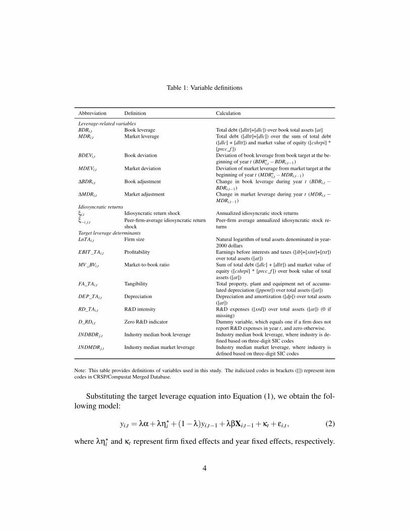
Table 1: Variable definitions

Abbreviation Definition Calculation

Leverage-related variablesBDRi,t Book leverage Total debt ([dltt]+[dlc]) over book total assets [at]MDRi,t Market leverage Total debt ([dltt]+[dlc]) over the sum of total debt

([dlc] + [dltt]) and market value of equity ([cshrpi] *[prcc_f ])

BDEVi,t Book deviation Deviation of book leverage from book target at the be-ginning of year t (BDR?

i,t −BDRi,t−1)MDEVi,t Market deviation Deviation of market leverage from market target at the

beginning of year t (MDR?i,t −MDRi,t−1)

∆BDRi,t Book adjustment Change in book leverage during year t (BDRi,t −BDRi,t−1)

∆MDRi,t Market adjustment Change in market leverage during year t (MDRi,t −MDRi,t−1)

Idiosyncratic returnsξi,t Idiosyncratic return shock Annualized idiosyncratic stock returnsξ−i, j,t Peer-firm-average idiosyncratic return

shockPeer-firm average annualized idiosyncratic stock re-turns

Target leverage determinantsLnTAi,t Firm size Natural logarithm of total assets denominated in year-

2000 dollarsEBIT _TAi,t Profitability Earnings before interests and taxes ([ib]+[xint]+[txt])

over total assets ([at])MV _BVi,t Market-to-book ratio Sum of total debt ([dlc] + [dltt]) and market value of

equity ([cshrpi] * [prcc_f ]) over book value of totalassets ([at])

FA_TAi,t Tangibility Total property, plant and equipment net of accumu-lated depreciation ([ppent]) over total assets ([at])

DEP_TAi,t Depreciation Depreciation and amortization ([dp]) over total assets([at])

RD_TAi,t R&D intensity R&D expenses ([xrd]) over total assets ([at]) (0 ifmissing)

D_RDi,t Zero R&D indicator Dummy variable, which equals one if a firm does notreport R&D expenses in year t, and zero otherwise.

INDBDR j,t Industry median book leverage Industry median book leverage, where industry is de-fined based on three-digit SIC codes

INDMDR j,t Industry median market leverage Industry median market leverage, where industry isdefined based on three-digit SIC codes

Note: This table provides definitions of variables used in this study. The italicized codes in brackets ([]) represent itemcodes in CRSP/Compustat Merged Database.

Substituting the target leverage equation into Equation (1), we obtain the fol-lowing model:

yi,t = λα+λη?i +(1−λ)yi,t−1 +λβXi,t−1 +κt + εi,t , (2)

where λη?i and κt represent firm fixed effects and year fixed effects, respectively.

4

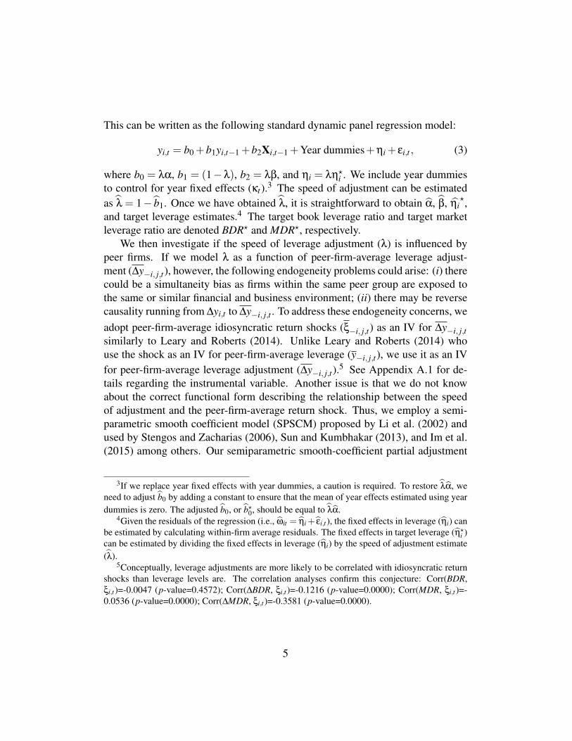
This can be written as the following standard dynamic panel regression model:

yi,t = b0 +b1yi,t−1 +b2Xi,t−1 +Year dummies+ηi + εi,t , (3)

where b0 = λα, b1 = (1−λ), b2 = λβ, and ηi = λη?i . We include year dummies

to control for year fixed effects (κt).3 The speed of adjustment can be estimatedas λ = 1− b1. Once we have obtained λ, it is straightforward to obtain α, β, ηi

?,and target leverage estimates.4 The target book leverage ratio and target marketleverage ratio are denoted BDR? and MDR?, respectively.

We then investigate if the speed of leverage adjustment (λ) is influenced bypeer firms. If we model λ as a function of peer-firm-average leverage adjust-ment (∆y−i, j,t), however, the following endogeneity problems could arise: (i) therecould be a simultaneity bias as firms within the same peer group are exposed tothe same or similar financial and business environment; (ii) there may be reversecausality running from ∆yi,t to ∆y−i, j,t . To address these endogeneity concerns, weadopt peer-firm-average idiosyncratic return shocks (ξ−i, j,t) as an IV for ∆y−i, j,tsimilarly to Leary and Roberts (2014). Unlike Leary and Roberts (2014) whouse the shock as an IV for peer-firm-average leverage (y−i, j,t), we use it as an IVfor peer-firm-average leverage adjustment (∆y−i, j,t).

5 See Appendix A.1 for de-tails regarding the instrumental variable. Another issue is that we do not knowabout the correct functional form describing the relationship between the speedof adjustment and the peer-firm-average return shock. Thus, we employ a semi-parametric smooth coefficient model (SPSCM) proposed by Li et al. (2002) andused by Stengos and Zacharias (2006), Sun and Kumbhakar (2013), and Im et al.(2015) among others. Our semiparametric smooth-coefficient partial adjustment

3If we replace year fixed effects with year dummies, a caution is required. To restore λα, weneed to adjust b0 by adding a constant to ensure that the mean of year effects estimated using yeardummies is zero. The adjusted b0, or b?0, should be equal to λα.

4Given the residuals of the regression (i.e., ωit = ηi+ εi,t ), the fixed effects in leverage (ηi) canbe estimated by calculating within-firm average residuals. The fixed effects in target leverage (η?

i )can be estimated by dividing the fixed effects in leverage (ηi) by the speed of adjustment estimate(λ).

5Conceptually, leverage adjustments are more likely to be correlated with idiosyncratic returnshocks than leverage levels are. The correlation analyses confirm this conjecture: Corr(BDR,ξi,t )=-0.0047 (p-value=0.4572); Corr(∆BDR, ξi,t )=-0.1216 (p-value=0.0000); Corr(MDR, ξi,t )=-0.0536 (p-value=0.0000); Corr(∆MDR, ξi,t )=-0.3581 (p-value=0.0000).

5

model (SPSCPAM) can be written as follows:

yi,t − yi,t−1 = φ(ξ−i, j,t)+λ(ξ−i, j,t)(y?i,t − yi,t−1)+ εi,t , (4)

where φ(·) and λ(·) are smooth but unknown functions of ξ−i, j,t . This approachwill allow us to know the functional form describing the relationship between thespeed of adjustment and the peer-firm-average return shock.

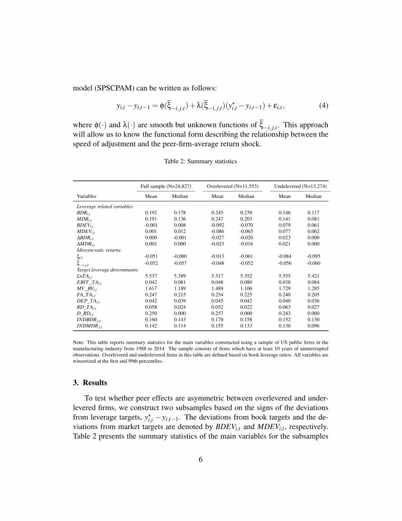
Table 2: Summary statistics

Full sample (N=24,827) Overlevered (N=11,553) Undelevered (N=13,274)

Variables Mean Median Mean Median Mean Median

Leverage related variablesBDRi,t 0.192 0.178 0.245 0.239 0.146 0.117MDRi,t 0.191 0.136 0.247 0.203 0.141 0.081BDEVi,t -0.001 0.008 -0.092 -0.070 0.079 0.061MDEVi,t 0.001 0.012 -0.086 -0.065 0.077 0.062∆BDRi,t 0.000 -0.001 -0.027 -0.020 0.023 0.000∆MDRi,t 0.001 0.000 -0.023 -0.016 0.021 0.000Idiosyncratic returnsξi,t -0.051 -0.080 -0.013 -0.061 -0.084 -0.095ξ−i, j,t -0.052 -0.057 -0.048 -0.052 -0.056 -0.060Target leverage determinantsLnTAi,t 5.537 5.389 5.517 5.352 5.555 5.421EBIT _TAi,t 0.042 0.081 0.048 0.080 0.038 0.084MV _BVi,t 1.617 1.189 1.489 1.106 1.729 1.285FA_TAi,t 0.247 0.215 0.254 0.225 0.240 0.205DEP_TAi,t 0.042 0.039 0.045 0.042 0.040 0.036RD_TAi,t 0.058 0.024 0.052 0.022 0.063 0.027D_RDi,t 0.250 0.000 0.257 0.000 0.243 0.000INDBDR j,t 0.160 0.143 0.170 0.158 0.152 0.130INDMDR j,t 0.142 0.114 0.155 0.133 0.130 0.096

Note: This table reports summary statistics for the main variables constructed using a sample of US public firms in themanufacturing industry from 1988 to 2014. The sample consists of firms which have at least 10 years of uninterruptedobservations. Overlevered and underlevered firms in this table are defined based on book leverage ratios. All variables arewinsorized at the first and 99th percentiles.

3. Results

To test whether peer effects are asymmetric between overlevered and under-levered firms, we construct two subsamples based on the signs of the deviationsfrom leverage targets, y?i,t − yi,t−1. The deviations from book targets and the de-viations from market targets are denoted by BDEVi,t and MDEVi,t , respectively.Table 2 presents the summary statistics of the main variables for the subsamples

6

of overlevered and underlevered firms as well as for the full sample. First, wefind that most key determinants of target leverage (i.e., firm size, profitability,asset tangibility, depreciation, R&D intensity and industry median leverage) arevery similar across the subsamples. However, we observe that growth opportuni-ties are somewhat different between the subsamples—underlevered firms tend tohave more growth opportunities. Second, we observe notable differences in theannualized idiosyncratic return shocks across subsamples. For example, mean id-iosyncratic return shocks are -1.3% and -8.4% for overlevered and underleveredfirms, respectively. Nevertheless, peer firm shocks measured as peer-firm-averageidiosyncratic return shocks are less noticeably different across the two subsam-ples. Mean peer firm shocks for overlevered and underlevered firms are -4.8%and -5.6%, respectively. Third, this table suggests that it is very important to in-vestigate overlevered and underlevered firms separately. For the full sample, bothmean book deviation and mean book adjustment are close to zero, but they arevery different from zero in the two subsamples. Mean book deviation for overlev-ered (underlevered) firms is -9.2% (7.9%), and mean book adjustment for over-levered (underlevered) firms is -2.7% (2.3%).6 Therefore, prior empirical resultsbased on the full sample should be interpreted with a caution as they may capturenet effects only when the results are asymmetric between the two subsamples.

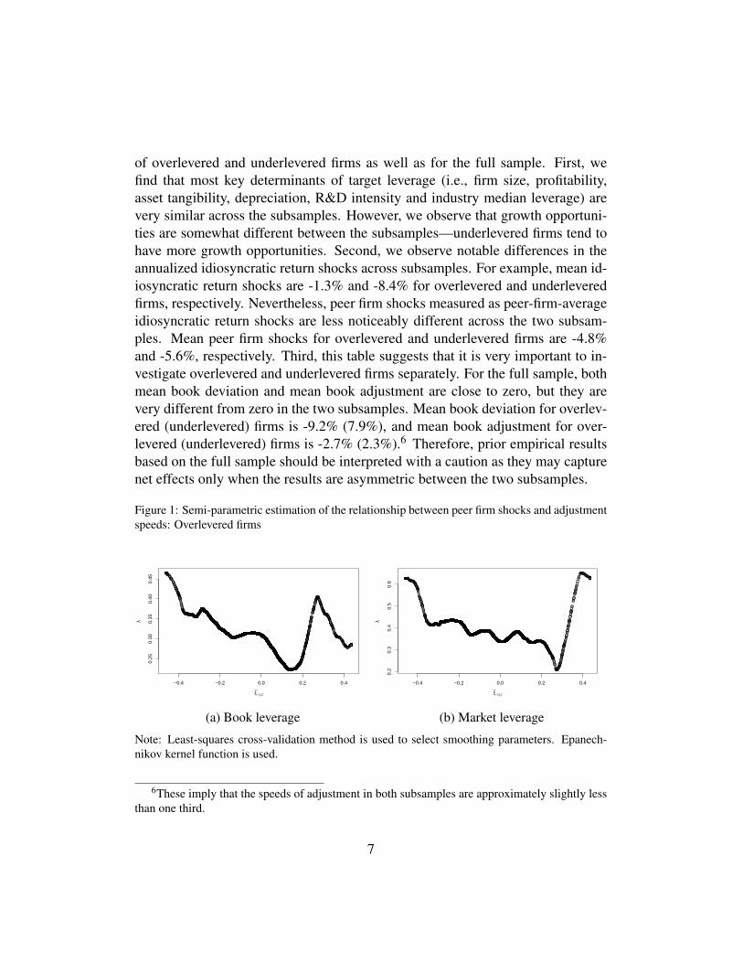
Figure 1: Semi-parametric estimation of the relationship between peer firm shocks and adjustmentspeeds: Overlevered firms

−0.4 −0.2 0.0 0.2 0.4

0.25

0.30

0.35

0.40

0.45

ξ−i,j,t

λ

(a) Book leverage

−0.4 −0.2 0.0 0.2 0.4

0.2

0.3

0.4

0.5

0.6

ξ−i,j,t

λ

(b) Market leverage

Note: Least-squares cross-validation method is used to select smoothing parameters. Epanech-nikov kernel function is used.

6These imply that the speeds of adjustment in both subsamples are approximately slightly lessthan one third.

7

Our main empirical results based on the estimation of SPSCPAMs stated inEquation (4) are presented below, separately for overlevered and underleveredfirms. Figure 1 reports the estimation results for the relationship between over-levered firms’ adjustment speeds (λ) and peer firm shocks (ξ−i, j,t). Panel (a)shows that overlevered firms’ book adjustment speeds and peer firm shocks havea quadratic, specifically U-shaped, relationship. This suggests that overleveredfirms adjust their leverage much faster when peer firms experience extremely badshocks or extremely good shocks compared with when peer firms experience mildshocks. Panel (b) shows that these phenomena are more pronounced for the mar-ket leverage measure.

When there are negative equity shocks to peers (e.g., default, scandals, law-suits, failure in patent applications), peer firms will lower their leverage faster thanwhen there are positive equity shocks to peers. After peer firms’ misfortunes suchas default or hostile takeover arise, shareholders of overlevered firms will forcemanagers to reduce the deviations from optimal leverage ratios. As influencedby peer firms’ failures, firms tend to converge to optima faster in terms of invest-ment, financing, and payout decisions. However, when there are positive shocksto peers, peer firms will increase the speed of leverage adjustment again but fordifferent reasons. When there are positive peer shocks (e.g., grant of patents, ap-pointment of a good CEO, resolution of a legal dispute), firms adjust their lever-age more quickly to avoid being financially distressed or being a target of hostiletakeovers driven by the loss of competitive advantage. The key assumption is thatfirms tend to have some “loose nuts and bolts” at times, but firms tend to tightenthose nuts and bolts after they observe peer firms’ serious misfortunes or whenthey are worried about the loss of competitiveness arising from peers’ fortunes.

Figure 2 reports the estimation results for the relationship between underlev-ered firms’ adjustment speeds (λ) and peer firm shocks (ξ−i, j,t). Panel (a) showsthat underlevered firms’ book adjustment speed monotonically increases with peerfirm shocks. In fact, the adjustment speed increases monotonically from 25% to38% as the shock to the peer firm moves away from negative, and becomes posi-tive. Panel (b) shows that a similar pattern is observed when we use market lever-age instead of book leverage, although there is more significant variation. Thissuggests that underlevered firms adjust their leverage very slowly when peer firmsexperience extremely bad shocks, but tend to adjust their leverage faster whenpeer firms face better shocks. One possible explanation for the low adjustmentspeed when peer shocks are negative is that an underlevered firm’s leverage is al-ready too low and is immune from this negative event such as default or a hostiletakeover, hence we do not observe any significant response from the management

8

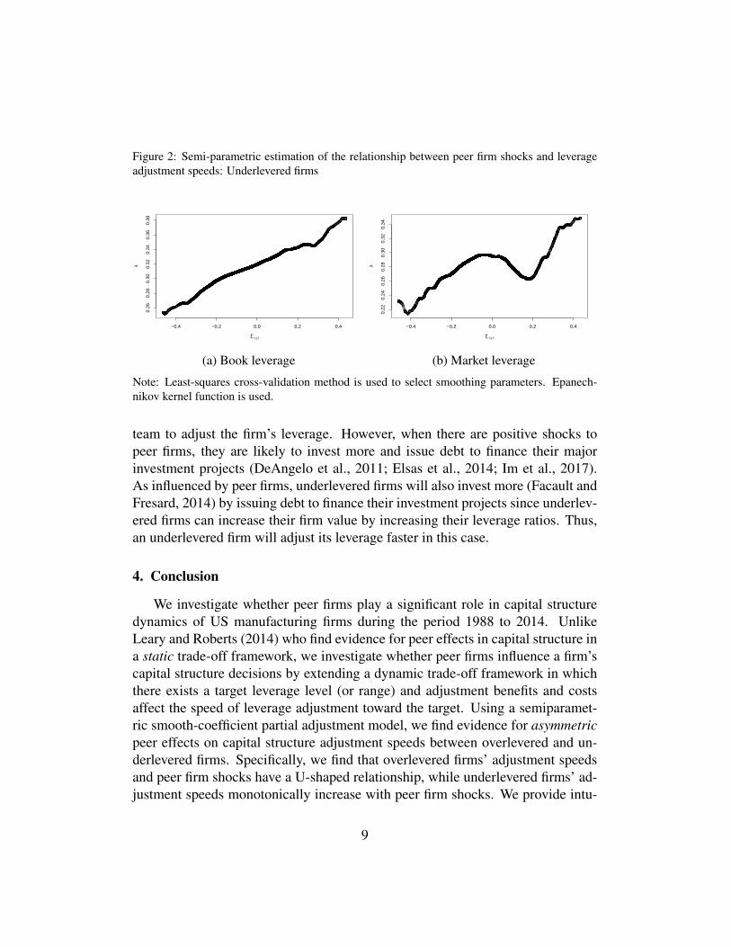
Figure 2: Semi-parametric estimation of the relationship between peer firm shocks and leverageadjustment speeds: Underlevered firms

−0.4 −0.2 0.0 0.2 0.4

0.26

0.28

0.30

0.32

0.34

0.36

0.38

ξ−i,j,t

λ

(a) Book leverage

−0.4 −0.2 0.0 0.2 0.4

0.22

0.24

0.26

0.28

0.30

0.32

0.34

ξ−i,j,t

λ

(b) Market leverage

Note: Least-squares cross-validation method is used to select smoothing parameters. Epanech-nikov kernel function is used.

team to adjust the firm’s leverage. However, when there are positive shocks topeer firms, they are likely to invest more and issue debt to finance their majorinvestment projects (DeAngelo et al., 2011; Elsas et al., 2014; Im et al., 2017).As influenced by peer firms, underlevered firms will also invest more (Facault andFresard, 2014) by issuing debt to finance their investment projects since underlev-ered firms can increase their firm value by increasing their leverage ratios. Thus,an underlevered firm will adjust its leverage faster in this case.

4. Conclusion

We investigate whether peer firms play a significant role in capital structuredynamics of US manufacturing firms during the period 1988 to 2014. UnlikeLeary and Roberts (2014) who find evidence for peer effects in capital structure ina static trade-off framework, we investigate whether peer firms influence a firm’scapital structure decisions by extending a dynamic trade-off framework in whichthere exists a target leverage level (or range) and adjustment benefits and costsaffect the speed of leverage adjustment toward the target. Using a semiparamet-ric smooth-coefficient partial adjustment model, we find evidence for asymmetricpeer effects on capital structure adjustment speeds between overlevered and un-derlevered firms. Specifically, we find that overlevered firms’ adjustment speedsand peer firm shocks have a U-shaped relationship, while underlevered firms’ ad-justment speeds monotonically increase with peer firm shocks. We provide intu-

9

itive explanations to our findings, although we agree that there may be alternativeexplanations.

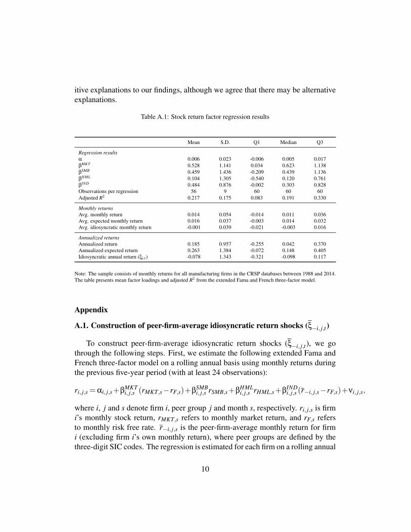
Table A.1: Stock return factor regression results

Mean S.D. Q1 Median Q3

Regression resultsα 0.006 0.023 -0.006 0.005 0.017βMKT 0.528 1.141 0.034 0.623 1.138βSMB 0.459 1.436 -0.209 0.439 1.136βHML 0.104 1.305 -0.540 0.120 0.761βIND 0.484 0.876 -0.002 0.303 0.828Observations per regression 56 9 60 60 60Adjusted R2 0.217 0.175 0.083 0.191 0.330

Monthly returnsAvg. monthly return 0.014 0.054 -0.014 0.011 0.036Avg. expected monthly return 0.016 0.037 -0.003 0.014 0.032Avg. idiosyncratic monthly return -0.001 0.039 -0.021 -0.003 0.016

Annualized returnsAnnualized return 0.185 0.957 -0.255 0.042 0.370Annualized expected return 0.263 1.384 -0.072 0.148 0.405Idiosyncratic annual return (ξi,t ) -0.078 1.343 -0.321 -0.098 0.117

Note: The sample consists of monthly returns for all manufacturing firms in the CRSP databases between 1988 and 2014.The table presents mean factor loadings and adjusted R2 from the extended Fama and French three-factor model.

Appendix

A.1. Construction of peer-firm-average idiosyncratic return shocks (ξ−i, j,t)

To construct peer-firm-average idiosyncratic return shocks (ξ−i, j,t), we gothrough the following steps. First, we estimate the following extended Fama andFrench three-factor model on a rolling annual basis using monthly returns duringthe previous five-year period (with at least 24 observations):

ri, j,s =αi, j,s+βMKTi, j,s (rMKT,s−rF,s)+β

SMBi, j,s rSMB,s+β

HMLi, j,s rHML,s+β

INDi, j,s (r−i, j,s−rF,s)+νi, j,s,

where i, j and s denote firm i, peer group j and month s, respectively. ri, j,s is firmi’s monthly stock return, rMKT,s refers to monthly market return, and rF,s refersto monthly risk free rate. r−i, j,s is the peer-firm-average monthly return for firmi (excluding firm i’s own monthly return), where peer groups are defined by thethree-digit SIC codes. The regression is estimated for each firm on a rolling annual

10

basis using historical monthly returns during the five-year period. We require atleast 24 months of historical data in the estimation. We compute expected returnsusing the estimated factor loadings and realized factor returns one year hence.We then compute idiosyncratic returns as the difference between realized returnsand expected returns. The regression results are summarized in Table A.1. Onaverage, adjusted R2 is as high as 21.7%. Mean idiosyncratic monthly return isaround -10 basis points, which is comparable to that in Leary and Roberts (2014).Second, we calculate firm i’s annualized idiosyncratic shocks in year t (ξi,t) asthe difference between annualized actual stock returns and annualized expectedstock returns. Finally, we calculate firm i’s peer-firm-average idiosyncratic returnshocks in year t (ξ−i, j,t) by taking the average of peer firms’ annualized year-tidiosyncratic shocks (excluding firm i’s).

A.2. Estimation of target leverage ratios

To implement the semiparametric smooth-coefficient partial adjustment modelstated in Equation (4), we first need to estimate target leverage ratios (y?i,t) and cal-culate the deviations from target leverage ratios (y?i,t − yi,t−1).7 As mentioned inSection 2, the estimation of leverage targets requires the estimation of a standarddynamic panel regression model stated in Equation (3). Note that there are sev-eral estimation issues arising from the simultaneous inclusion of fixed effects andlagged dependent variables. For instance, the ordinary least squares (OLS) andwithin groups (WG) estimates of the coefficient of the lagged dependent variabletend to be biased upwards and downwards, respectively. This is particularly truewhen the data have a short panel length (Nickell, 1981; Bond, 2002). There-fore, the coefficients of Xi,t−1 in Equation (2) are also likely to be biased. Usingsimulated panel data, Flannery and Hankins (2013) show that the estimation per-formance of various econometric methodologies varies substantially dependingon data complications, such as fixed effects, the persistence of the dependent vari-able, endogenous independent variables, and error term autocorrelations. Theyfind that the LSDVC estimator proposed by Bruno (2005) performs the best inthe absence of endogenous independent variables whereas the System GMM es-timator (Arellano and Bover, 1995; Blundell and Bond, 1998) appears to be the

7As in Faulkender et al. (2012), we first estimate target leverage ratios before estimating thespeed of leverage adjustment. Unlike Faulkender et al. (2012) who use a parametric partial ad-justment model to estimate adjustment speeds, we employ a semiparametric partial adjustmentmodel.

11

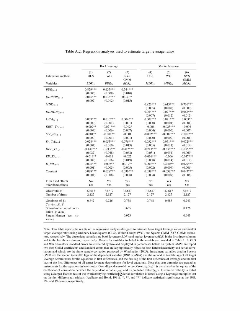
Table A.2: Regression analyses used to estimate target leverage ratios

Book leverage Market leverage

(1) (2) (3) (4) (5) (6)Estimation method OLS WG SYS

GMMOLS WG SYS

GMMVariables BDRi,t BDRi,t BDRi,t MDRi,t MDRi,t MDRi,t

BDRi,t−1 0.829*** 0.637*** 0.744***(0.005) (0.008) (0.010)

INDBDR j,t−1 0.045*** 0.038*** 0.030**(0.007) (0.012) (0.015)

MDRi,t−1 0.823*** 0.613*** 0.736***(0.005) (0.008) (0.009)

INDMDR j,t−1 0.054*** 0.077*** 0.063***(0.007) (0.012) (0.013)

LnTAi,t−1 0.003*** 0.010*** 0.004*** 0.002*** 0.021*** 0.003**(0.000) (0.001) (0.001) (0.000) (0.001) (0.001)

EBIT _TAi,t−1 -0.009** -0.021*** -0.012* -0.006 -0.023*** -0.004(0.004) (0.006) (0.007) (0.004) (0.006) (0.007)

MV _BVi,t−1 -0.001** -0.001** -0.001 -0.002*** -0.002*** -0.002***(0.000) (0.001) (0.001) (0.000) (0.000) (0.001)

FA_TAi,t−1 0.028*** 0.053*** 0.076*** 0.032*** 0.071*** 0.072***(0.004) (0.010) (0.013) (0.005) (0.011) (0.014)

DEP_TAi,t−1 -0.149*** -0.213*** -0.412*** -0.213*** -0.238*** -0.475***(0.027) (0.048) (0.062) (0.031) (0.051) (0.069)

RD_TAi,t−1 -0.019** -0.011 -0.022 -0.036*** -0.006 -0.047***(0.009) (0.016) (0.019) (0.008) (0.014) (0.017)

D_RDi,t−1 0.005*** 0.007** 0.012** 0.009*** 0.010** 0.029***(0.001) (0.003) (0.005) (0.002) (0.004) (0.006)

Constant 0.028*** 0.028*** 0.036*** 0.038*** -0.032*** 0.043***(0.004) (0.008) (0.008) (0.004) (0.009) (0.008)

Firm fixed effects No Yes Yes No Yes YesYear fixed effects Yes Yes Yes Yes Yes Yes

Observations 32,617 32,617 32,617 32,617 32,617 32,617Number of firms 2,127 2,127 2,127 2,127 2,127 2,127

Goodness-of-fit—Corr(yi,t , yi,t)

20.742 0.726 0.738 0.748 0.683 0.743

Second-order serial corre-lation (p-value)

0.655 0.176

Sargan-Hansen test (p-value)

0.923 0.943

Note: This table reports the results of the regression analyses designed to estimate book target leverage ratios and markettarget leverage ratios using Ordinary Least Squares (OLS), Within Groups (WG), and System GMM (SYS GMM) estima-tors, respectively. The dependent variables are book leverage (BDR) and market leverage (MDR) in the first three columnsand in the last three columns, respectively. Details for variables included in the models are provided in Table 1. In OLSand WG estimators, standard errors are clustered by firm and displayed in parentheses below. In System GMM, we reporttwo-step GMM coefficients and standard errors that are asymptotically robust to both heteroskedasticity and serial corre-lation, and which use the finite-sample correction proposed by Windmeijer (2005). Instrument variables used in SystemGMM are the second to twelfth lags of the dependent variable (BDR or MDR) and the second to twelfth lags of all targetleverage determinants for the equations in first-differences, and the first lag of the first-difference of leverage and the firstlags of the first-differences of all target leverage determinants for level equations. Note that year dummies are treated asinstruments for the equations in levels only. Overall goodness-of-fit score, Corr(yi,t , yi,t)

2, is calculated as the square of thecoefficient of correlation between the dependent variable (yi,t ) and its predicted value (yi,t ). Instrument validity is testedusing a Sargan-Hansen test of the overidentifying restrictions. Serial correlation is tested using a Lagrange multiplier teston the first-differenced residuals (Arellano and Bond, 1991). *, **, and *** indicate statistical significance at the 10%,5%, and 1% levels, respectively.

12

best choice in the presence of endogeneity and even second-order serial correla-tion if the dataset includes shorter panels. We reports the results based on thethree econometric methodologies to highlight that the results are significantly in-fluenced by the choice of estimation methods, but we use the System GMM resultsto estimate target leverage ratios.

Our regression results are reported in Table A.2. Columns 1–3 and Columns4–5 present the estimation results for book and market leverage ratios, respec-tively. For each leverage measure, we report estimation results based on OLS,WG, and System GMM estimators. We include year fixed effects to account fortemporal variations in all three specifications. The System GMM results are sat-isfactory for the following reasons. First, the coefficients of the lagged dependentvariable estimated by the System GMM lies between the OLS and WG estimates,as predicted by Nickell (1981) and Bond (2002). Second, the goodness-of-fitscores of the System GMM model are higher than those of the WG model andslightly lower than those of the OLS model. Note that the goodness-of-fit scoreshould be lower in the WG and System GMM models than in the OLS modelas a term reflecting unobserved heterogeneity is a component of the error termin the WG and System GMM models. Third, Arellano and Bond’s (1991) serialcorrelation tests find no significant evidence of the second-order serial correla-tion in the first-differenced residuals (p-value=0.655 for BDR; p-value=0.176 forMDR). Finally, Sargan-Hansen tests of overidentifying restrictions do not rejectthese specifications (p-value=0.923 for BDR; p-value=0.943 for MDR). Overall,the signs of the main determinants of leverage targets are consistent with theoret-ical predictions. Size, asset tangibility, zero R&D indicator, and industry medianleverage are positively associated with the target leverage estimates. Profitability,market-to-book, non-debt tax shield proxies, and R&D intensity are all negativelyassociated with the target estimates generally in all regression models. Most ofthe relationships are consistent with the findings of the related literature, i.e., Famaand French (2002), Flannery and Rangan (2006), and Faulkender et al. (2012).

13

References

Arellano, M., Bond, S., 1991. Some tests of specification for panel data: Montecarlo evidence and an application to employment equations. The Review ofEconomic Studies 58 (2), 277–297.

Arellano, M., Bover, O., 1995. Another look at the instrumental variable estima-tion of error-components models. Journal of Econometrics 68 (1), 29–51.

Blundell, R., Bond, S., 1998. Initial conditions and moment restrictions in dy-namic panel data models. Journal of Econometrics 87 (1), 115–143.

Bond, S. R., 2002. Dynamic panel data models: a guide to micro data methodsand practice. Portuguese Economic Journal 1 (2), 141–162.

Bruno, G. S., 2005. Approximating the bias of the LSDV estimator for dynamicunbalanced panel data models. Economics Letters 87 (3), 361–366.

Cook, D. O., Tang, T., 2010. Macroeconomic conditions and capital structureadjustment speed. Journal of Corporate Finance 16 (1), 73–87.

DeAngelo, H., DeAngelo, L., Whited, T. M., 2011. Capital structure dynamicsand transitory debt. Journal of Financial Economics 99 (2), 235–261.

Elsas, R., Flannery, M. J., Garfinkel, J. A., 2014. Financing major investments:information about capital structure decisions. Review of Finance 18 (4), 1341–1386.

Fama, E. F., French, K. R., 2002. Testing trade-off and pecking order predictionsabout dividends and debt. The Review of Financial Studies 15 (1), 1–33.

Faulkender, M., Flannery, M. J., Hankins, K. W., Smith, J. M., 2012. Cash flowsand leverage adjustments. Journal of Financial Economics 103 (3), 632–646.

Faulkender, M., Yang, J., 2010. Inside the black box: The role and composition ofcompensation peer groups. Journal of Financial Economics 96 (2), 257–270.

Fischer, E. O., Heinkel, R., Zechner, J., 1989. Dynamic capital structure choice:Theory and tests. The Journal of Finance 44 (1), 19–40.

14

Flannery, M. J., Hankins, K. W., 2013. Estimating dynamic panel models in cor-porate finance. Journal of Corporate Finance 19, 1–19.

Flannery, M. J., Rangan, K. P., 2006. Partial adjustment toward target capital struc-tures. Journal of Financial Economics 79 (3), 469–506.

Foucault, T., Fresard, L., 2014. Learning from peers’ stock prices and corporateinvestment. Journal of Financial Economics 111 (3), 554–577.

Frank, M. Z., Goyal, V. K., 2009. Capital structure decisions: which factors arereliably important? Financial Management 38 (1), 1–37.

Graham, J. R., Harvey, C. R., 2001. The theory and practice of corporate finance:Evidence from the field. Journal of Financial Economics 60 (2), 187–243.

Hovakimian, A., Opler, T., Titman, S., 2001. The debt-equity choice. Journal ofFinancial and Quantitative Analysis 36 (1), 1–24.

Huang, R., Ritter, J. R., 2009. Testing theories of capital structure and estimatingthe speed of adjustment. Journal of Financial and Quantitative Analysis 44 (2),237–271.

Hunter, D., Kandel, E., Kandel, S., Wermers, R., 2014. Mutual fund perfor-mance evaluation with active peer benchmarks. Journal of Financial Economics112 (1), 1–29.

Im, H. J., Mayer, C., Sussman, O., 2017. Investment spike financing.

Im, H. J., Park, Y. J., Shon, J., 2015. Product market competition and the value ofinnovation: Evidence from US patent data. Economics Letters 137, 78–82.

Kaustia, M., Knüpfer, S., 2012. Peer performance and stock market entry. Journalof Financial Economics 104 (2), 321–338.

Leary, M. T., Roberts, M. R., 2005. Do firms rebalance their capital structures?The Journal of Finance 60 (6), 2575–2619.

Leary, M. T., Roberts, M. R., 2014. Do peer firms affect corporate financial pol-icy? The Journal of Finance 69 (1), 139–178.

Li, Q., Huang, C. J., Li, D., Fu, T.-T., 2002. Semiparametric smooth coefficientmodels. Journal of Business & Economic Statistics 20 (3), 412–422.

15

Manski, C. F., 1993. Identification of endogenous social effects: The reflectionproblem. The Review of Economic Studies 60 (3), 531–542.

Nickell, S., 1981. Biases in dynamic models with fixed effects. Econometrica:Journal of the Econometric Society, 1417–1426.

Öztekin, Ö., Flannery, M. J., 2012. Institutional determinants of capital structureadjustment speeds. Journal of Financial Economics 103 (1), 88–112.

Stengos, T., Zacharias, E., 2006. Intertemporal pricing and price discrimination:a semiparametric hedonic analysis of the personal computer market. Journal ofApplied Econometrics 21 (3), 371–386.

Sun, K., Kumbhakar, S. C., 2013. Semiparametric smooth-coefficient stochasticfrontier model. Economics Letters 120 (2), 305–309.

Welch, I., 2004. Capital structure and stock returns. Journal of Political Economy112 (1), 106–131.

Windmeijer, F., 2005. A finite sample correction for the variance of linear efficienttwo-step GMM estimators. Journal of Econometrics 126 (1), 25–51.

16