ASYMMETRIC ADJUSTMENTS OF PRICE AND OUTPUT

P.A. Tinsley and Reva Krieger�

version: June 1997

Abstract: Asymmetries in price adjustment can reconcile contrasts between rapid price movements ininflationary episodes, consistent with classical theories of flexible pricing, and sluggish price responsesin contractions, consistent with Keynesian theories of sticky price adjustments. Nonparametric analysisof SIC two-digit industry data indicates that negative asymmetries are more pronounced for real outputsthan for nominal outputs, suggesting reversed positive asymmetries in producer pricing. Pricing decisionrules are estimated to distinguish between asymmetries in conditioning shocks and asymmetries in producerresponses. Two rational motives for asymmetric pricing are supported.

Keywords: Asymmetric trend deviations, rational error correction, producer pricing.

�Authors' addresses are: Federal Reserve Board, Washington, D.C. 20551, ptinsley@frb.gov; and InternationalMonetary Fund, Washington, D.C. 20431, rkrieger@imf.org. Views presented are those of the authors and do notnecessarily represent those of the Federal Reserve Board or the International Monetary Fund. Our thanks to R.Sweeney and two referees for useful suggestions. Forthcoming inEconomic Inquiry.

1

I. INTRODUCTION

A sharp difference persists in economics regarding the dynamic adjustments of prices.

In classical theories, markets are continuously cleared by flexible prices with instantaneous

adjustments of prices to agents' perceptions of monetary policy. In contrast, Keynesian theories

suggest non-auction prices are slow to adjust to equilibrium with short-run clearing achieved by

adjustments of transacted quantities. A sufficient reason for the continued split in descriptions is

that both views are supported by empirical evidence. The case for sticky prices is not easily squared

with the rapid movements of prices in inflationary episodes, as reviewed by Sargent [1982]. On the

other hand, the assumption of instantaneously flexible producer prices seems inconsistent with the

lengthy spells of rigid prices documented in Carlton [1986] and Blinder [1991] and the sluggish

price responses estimated by Sims [1992] and Christiano, Eichenbaum, and Evans [1994].

A third alternative is that both classical and Keynesian characterizations may be describing

price behavior in different stages of business cycles if producers respond asymmetrically to positive

and negative deviations from trends. Prompt producer corrections of prices that are below trends

can account for the essential classical feature of flexible price responses to expected inflation.

Conversely, resistance to margin reductions for prices that are above trends can support the

Keynesian description of sluggish adjustment that leaves prices at excessively high levels over

extended intervals.1

This paper examines the case for asymmetric pricing in four steps:

� A recent literature, vid. Sichel [1993], indicates that manufacturing output exhibits various

negative asymmetries, such as larger trend deviations (in absolute value) at cyclical troughs

than at peaks. In section II, a search for similar asymmetries in the outputs of SIC two-digit

industries finds that negative asymmetries in trend deviations are more pronounced in real

outputs than in nominal outputs. This suggests an offsetting positive asymmetry in industry

prices where below-trend prices are more readily raised than above-trend prices are lowered.

� Although suggestive, reported measures of asymmetric data features are atheoretic so sources

of asymmetric behavior are ambiguous. To help distinguish between the roles of exogenous

shocks and endogenous responses in producer pricing, benchmark structural models of

symmetric pricing are examined in section III. The standard frictions model of gradual price

corrections based on costly adjustment of price levels, such as Rotemberg [1982; 1987], is

rejected for prices of manufacturing industries. Empirical models of industry pricing appear to

be consistent with an extended definition of frictions where producers aim to smooth moving

averages of prices and inflation rates.

1Although short-run inflexibility of nominal prices is a tenet of new-Keynesian theories of business cyclecontractions, an awkward implication of symmetrically sticky price models is that prices may get stuck also at levelsthat are too low for market clearing.

2

� The extended frictions model of symmetric pricing is then used in section IV to identify sources

of asymmetries in producer pricing. Empirical tests indicate that the effects of trend deviations

in output on price adjustments are either statistically insignificant or inconsistent with positive

asymmetries in pricing, and that asymmetric pricing appears to be a structural decision that

depends on whether the industry price is below or above its trend.

� Section V reviews several interpretations of asymmetric pricing and suggests a representative

indicator for each theory. Industry values of these indicators are compared with industry

estimates of asymmetric pricing; the cross-industry correlations support two rational motives

for positive asymmetries in producer pricing. Section VI concludes.

II. ASYMMETRIES IN INDUSTRY OUTPUT

This section presents nonparametric measures of asymmetric behavior in output. In contrast

to previous work on macroeconomic aggregates, discussion is aimed at outputs of SIC two-digit

industries in manufacturing. A comparison between real and nominal outputs is also introduced

which suggests an asymmetry in industry pricing.

Descriptions of asymmetric behavior were prominent in prewar business cycle literature, such

as Mitchell [1927], Means [1935], and Haberler [1938]. The issue of cyclical asymmetries then

fell into disfavor with the postwar emergence of models of agent behavior based on stochastic

linear difference equations. However, over the last decade, several studies have resuscitated

atheoretic measurement of cycle asymmetries, with mixed findings for asymmetry. Neftci [1984]

presents evidence of asymmetry in the aggregate rate of unemployment, with unemployment

faster to rise and slower to fall. Falk [1986] and DeLong and Summers [1986] confirm the

positive asymmetry in the unemployment rate but find no evidence of matching asymmetries in

the movements of detrended GNP. By contrast, Goodwin and Sweeney [1993] provide evidence

of negative asymmetry in real GNP growth where positive growth rates are constrained by a real

output ceiling, as suggested by Friedman [1993]. Because the amplitudes of cyclical fluctuations

are larger in goods than in services, recent analyses of McNevin and Neftci [1991], McQueen

and Thorley [1993], and Sichel [1993] examine cyclical movements in industrial production and

indicate that the behavior of goods output appears to be different in recessions than in expansions.

The patterns of asymmetric movements reported for aggregate output vary by study, in part due

to different definitions of asymmetry. The premise advanced by Mitchell [1927] is that output falls

faster from cyclical peak to trough than in the expansion from trough to peak. Termed “steepness”

asymmetry by Sichel [1993], a pattern of slow ascents and rapid descents will be described here as

negativegrowth rate asymmetry. Asymmetries in positive and negative growth rates of detrended

output are supported for production of durable goods in McNevin and Neftci [1991] but rejected

for total industrial production by Sichel [1993].

3

A contrasting pattern of cyclical asymmetry was suggested by the nonlinear business cycle

model of Hicks [1950] where output expansions are eventually constrained by capacity ceilings

due to shortages of labor or fixed capital. Because capacity ceilings place upper bounds on output

growth in expansions that are not matched by comparable lower bounds on output contractions

in recessions, the average squared negative deviation from trend may exceed the average squared

positive deviation from trend.2 Sichel [1993] indicates that trend deviations at troughs are larger (in

absolute value) than trend deviations at peaks for industrial production, depending on the method

of detrending. Dubbed “deepness” asymmetry by Sichel, this pattern is described here as negative

gap asymmetry, to emphasize that this is a pattern of trend deviations in log levels rather than in

log differences.

The analysis of industry outputs that follows is directed at three unresolved issues:

� First, are asymmetries reported for aggregate goods output also reproduced in industry

disaggregations? If asymmetric motion is only apparent in total goods output then it is unlikely

to be an intrinsic characteristic of producer behavior but a result of aggregation, perhaps due to

cyclical shifts in the composition of aggregate demand.

� Second, are either of the asymmetric patterns catalogued by Sichel [1993] pervasive in

industry behavior? As indicated later, if displacements away from a trend are due largely to

unanticipated shocks then asymmetry in gaps on different sides of the trend, due to different

producer responses to positive and negative shocks, is amenable to structural interpretations.

By contrast, asymmetry in detrended growth rates is more difficult to rationalize in a

typical shock/response model of behavior because the set of positive (negative) growth rates

encompasses both the return from a trough (peak) turning point to the trend and the subsequent

departure from the trend to the next peak (trough).

� Third, if systematic asymmetries are detected in industry outputs, are they also reproduced in

nominal output? If the same asymmetries in real output are reproduced in nominal output then

an intrinsic asymmetry in producer pricing, such as the “administered pricing” conjecture of

Means [1935], is unlikely to be an important cause of cyclical asymmetries in output.

Selecting the Trends of Industry Outputs and Prices.

Although the empirical literature cited above presents evidence of asymmetries in economic

time series, there does not appear to be a consensus among economists that asymmetric responses

are a fundamental characteristic of agent behavior. In the case of trending variables, a sufficient

reason for scepticism is that empirical evidence of asymmetries appears to depend on the method

2Asymmetry in squared deviations is not inconsistent with standard detrending constructions that yield equal sums(in absolute value) of negative and positive trend deviations.

4

of detrending, vid. Canova [1993]. If the true trend is overstated then the average of negative

deviations from trend will tend to exceed the average of positive deviations, biasing results towards

a finding of negative asymmetry, and vice versa for underestimates of the trend. The analytical

focus of the literature on asymmetric trend deviations is further blurred by the wide assortment of

available detrending methods.3

In the case of manufacturing industries, postwar time series on industry outputs and prices are

consistent with difference-stationary behavior so it appears appropriate to select I(1) trends that

are cointegrated with the relevant industry prices and outputs. For log industry output,qt, the trend

measures used here are based on FRB staff estimates of capacity utilization, Raddock [1985]. The

industry log utilization rates are stationary, so the sample mean of an industry utilization rate may

be interpreted as the long-run preferred utilization rate of producers. Trend output or the log of

preferred output,q�t , is constructed by subtracting the log of the industry utilization rate from log

output,q�t � qt � ut. The log of the preferred utilization rate is normalized to zero by removing

the sample mean to ensure that the sum of sample trend deviations is zero,P

t ut = 0.

The log of industry nominal output,nt, is the sum of log output plus log price,nt = qt + pt.

Under imperfect competition by identical producers, the optimal industry price can be expressed

as a markup over marginal cost.4 Under the assumption that gross production is Cobb-Douglas,

the log price trend,p�, of each industry is constructed by cointegration regressions on weighted

indexes of the log prices of raw and intermediate materials inputs and unit labor costs, where

the index weights reflect the input requirements of the relevant industry. As one would hope for

exogenous trend constructions, vid. Gonzalo and Granger [1995], systematic reductions in the

trend deviations of both industry price and output are dominated by the error correction responses

of industry price,�pt, and output,�qt, whereas error correction responses of trend price,�p�t ,

and trend output,�q�t , are negligible.5

Contrasts of real and nominal output trend deviations.

Asymmetries in trend deviations by industry real and nominal output are displayed in table I.

The basic measure of asymmetry in table I is the ratio of the positive semi-variance (the mean of

squared positive deviations from trend) to the negative semi-variance (the mean of squared negative

3Cautions against indiscriminate use of detrending methods include those of Nelson and Kang [1981] ondeterministic trends, Osborn [1993] on detrending by moving average filters, and Harvey and Jaeger [1993] ondetrending by the Hodrick-Prescott filter.

4In standard formulations, such as Waterson [1984], the log margin islog[1� (s�)�1]�1 where� denotes the priceelasticity of industry demand ands is the number of producers, illustrating monoply or competitive solutions ass! 1or s!1

5An appendix on the integration orders, cointegrating trends, and error correction responses of industry prices andoutputs is available from the authors.

5

deviations from trend). The entries in table I will be one if the distribution of trend deviations is

symmetrical but less than one if the distribution is negatively skewed.6

Negative asymmetry in growth rates is rejected for detrended real GNP by DeLong and

Summers [1986] and Sichel [1993]. The first two columns of table I indicate the extent of

asymmetry in the growth rates of detrended industry outputs,�qt � �q�t . Trend output,q�t , is

measured in the first column by a simple linear trend, labeledOLS trend, and in the second column

by the cointegrating construction based on FRB capacity utilization rates, labeledI(1) trend.

Negative asymmetry in growth rates appears to be reasonably widespread among manufacturing

industries, and the degree of asymmetry is relatively insensitive to the choice of trend. The ratio of

positive to negative semi-variances for the growth rates of real output is less than unity at a90%

significance level or better for seven industries and considerably less than unity for all but three or

four industries.

The third column in table I displays the ratio of semi-variances in the growth rates of trend

deviations in industry nominal outputs. Here, there appears to be much less evidence of negative

asymmetry in growth rates. The semi-variance ratios for nominal output are generally larger

than those for real output and about a third of the ratios are greater than one, indicating that the

positive growth rates of detrended nominal output are larger than the negative growth rates in those

industries.

The right half of table I displays asymmetries in the levels of trend deviations where the relevant

measure is the gap deviation,qt � q�t . As with the growth rate measures, the first two columns in

the right half of table I measure the asymmetry in squared output gaps for two measures of trend

in output. In the case of the linearOLS trend, there is no clear tendency towards negative gap

asymmetry with about half of the industries above one and the remainder below. However, because

OLS regressions minimize the sum of squared deviations, the linear trend is biased against gap

asymmetry. Even if negative gap asymmetry exists, the OLS estimator pulls down the estimated

trend in order to reduce the squared outlier effects of the larger negative gaps.

A different picture emerges in the next column of table I, labeledI(1) trend, which uses the

cointegrating trends based on preferred utilization of capacity output. This measure suggests

negative gap asymmetry in output is even more pervasive across industries than the asymmetry

of growth rates shown in the first half of the table. The ratio of the semi-variances of positive trend

gaps to negative trend gaps is less than one for all but one industry. More striking than the general

incidence of negative gap asymmetry is the severity of the average shortfall from trend utilization

6Let �t denote a deviation from trend in periodt. As noted earlier, the mean trend deviation is zero by construction,Pt �t = 0. Asymmetry in “gaps” is measured by the ratio of the mean of squared positive deviations to the mean of

squared negative deviations,(P

t[�+

t ]2=n+)=(

Pt[�

�

t ]2=n�), where there aren+ positive trend deviations,�+t > 0,

andn� negative trend deviations,��t < 0. Asymmetry in growth rates is similarly measured by the ratio of the meanof squared positive first-differences in the trend deviations to the mean of squared negative first-differences.

6

of capacity production that occurs in many industries. In about half of the industries, the average

squared negative output gap is more than double the size of the average squared positive output

gap.

The last column in table I shows asymmetry gap measures for industry nominal output. The

incidence of negative asymmetry is much less evident for nominal output. By contrast with the

measure for real output in the preceding column, the measure of gap asymmetry for nominal output

moves toward or past unity for most industries, and negative gap asymmetry remains statistically

significant for only three industries.

The finding that negative gap asymmetry is more pervasive and marked for real output than

for nominal output also suggests a reverse positive asymmetry in pricing. If industry price is

symmetrically sluggish about its own trend, we might expect the gap asymmetry in real output to

be more-or-less reproduced in nominal output. The fact that negative gap asymmetry in nominal

output is generally much closer to unity or even replaced by positive asymmetry suggests that

negative asymmetries in real output are often matched by positive asymmetries in prices, yielding

more symmetric distributions for nominal output gaps.

Although results in table I indicate sizable asymmetries in the production and pricing of

manufacturing producers, it is important to not overinterpret what can be established by atheoretic

measurement. Negative gap asymmetry for output may indicate that the average negative shock

to output is larger than the average positive shock or that production is slower to recover from

adverse shocks. Indeed, in the absence of an articulated model of producer behavior, it is not clear

whether motion away from trends represent unforeseen displacements due to shocks or planned

overshooting of trends by producers.

To reduce such ambiguities associated with atheoretic analysis, the remainder of the paper

explores possible sources of asymmetries using structural models of producer behavior. Specific

dynamic optimality conditions will be discussed in some detail later. However, a brief preview of

this structural framework is provided by a representative Euler condition for optimal adjustment of

a producer decision variable such as output or price

Etff(yt�i; yt; yt+ij�)� y�t g = 0; (1)

wheref(:) is a two-sided function of leads and lags in the decision variable,y; � denotes the

parameters off(:) that are shaped largely by the nature of the frictions or “adjustment costs”

that confront producers; and the forcing term of the Euler equation,y�t , is the effective trend or

long-run target of the decision variable. In the absence of adjustment costs,f(:) � yt, and the

expected gap or trend deviation,Etfyt � y�t g, is zero. This simple structural model of producer

behavior suggests two sources of asymmetries in realized gaps. One is exogenous and stems from

7

potential asymmetries in unpredictable shocks to the forcing term; the other is endogenous due to

asymmetric responses by producers, captured by state-conditional movements in the parameters of

the Euler equation,�.

Output, price, or both may be viewed as the effective instrument(s) of producers. The remainder

of this paper focuses on friction models of pricing,yt � pt. The reason for this is the evidence

in table I that many industries exhibit both negative gap asymmetries in output and positive gap

asymmetries in pricing. If output movements capture the original source of asymmetry then

the negative asymmetry in output should be able to explain the positive asymmetry in pricing.

An alternative conjecture is that resistance to downward adjustments of nominal prices, as in

Means [1935] and Tobin [1972], may exacerbate contractions of industry production in recessions.

This interpretation suggests an endogenous characterization of asymmetric pricing where the

parameters of linear pricing rules,�, exhibit asymmetric responses to positive and negative trend

deviations in price. Tests of both interpretations of asymmetric pricing are discussed in a later

section.

III. STRUCTURAL MODELS OF SYMMETRIC PRICE ADJUSTMENTS

Although the final goal of this paper is to identify asymmetries in pricing, this section first

develops a symmetric pricing model to be used as a testbed for asymmetric variations. Without a

reasonable benchmark model, estimated asymmetries could plausibly be attributed to features of

uninteresting ad hoc fixes, such as autocorrelated errors.

The standard frictions model of gradual price responses, such as Rotemberg [1982; 1987],

is based on costly adjustment of price levels. The initial subsection shows that the standard

model is not supported by manufacturing prices, where empirical problems include substantial

residual autocorrelation and rejection of the overidentifying restrictions associated with rational

expectations. The second subsection develops a more general model of frictions in dynamic pricing

that appears to be accepted by industry data.

Rational pricing under quadratic costs of adjusting levels.

By construction, a cointegrating target price path,p�t , is an equilibrium objective for the

industry price,pt, in the absence of stochastic shocks. However, once displaced from the target

path, due to errors in estimating costs or demand, various frictions or dynamic market strategies

may impede an immediate return to the target path.

A tractable description of gradual price adjustments is provided by Rotemberg [1982; 1987]

where a second-order expansion of profits about an equilibrium profit-maximizing price represents

producers as minimizing the discounted sum of squared deviations about the equilibrium price path

8

and the cost of squared changes in the level of the price.

pt = argmin

Etf

1Xi=0

Bi[b0(pt+i � p�t+i)2 + b1(pt+i � pt+i�1)

2]g

!; (2)

whereEtf:g denotes producer expectations given information throught� 1, andB is a (quarterly)

discount factor.7

The associated first-order condition for optimal price adjustment is described by a second-order

Euler equation, written here as a function of two first-order polynomials in lag,L, and leadF ,

operators whereLxt = xt�1 andFxt = xt+1.

EtfA(BF )A(L)pt � A(1)A(B)p�tg = 0: (3)

On the left-hand-side of3, A(L) denotes the first-order polynomial in the lag operator,A(L) �

(1��L), andA(BF ) is the matching factor polynomial in the lead operator. These polynomials are

balanced on the other side of the minus sign by the sums of the polynomial weights,A(1) � 1� �

andA(B) � 1� �B.8

As is well-known, e.g., Tinsley [1970b], the optimal decision rule under quadratic adjustment

costs can be written as a partial adjustment of the decision instrument towards a moving target.

Multiplying equation3 by the inverse of the lead polynomial,A(BF )�1, and rearranging gives

�pt = EtfA(1)A(B)A(BF )�1p�t + (�pt � A(L)pt)g; (4)

= A(1)A(B)Etf1Xi=0

(�B)ip�t+ig � A(1)pt�1;

= A(1)[St(�B; p�)� pt�1];

whereSt(:) denotes the moving target of discounted forward trend prices.9

In the case of I(1) difference-stationary variables, such as the industry prices considered here,

the decision rule in equation4 can be reformulated also as arational error correction rule, Tinsley

[1993]. To show this, we first identify the unobserved expectations,Etf:g, by assuming that agents'

7B is set to:98, approximating the postwar annual real return to equity of about8 percent. No empirical results inthis paper are overturned by modest variations inB.

8The characteristic roots of 3 are� and(�B)�1, where� is the fractional root of the equation,(1 � �B)(��1 �1)� b0=b1 = 0. This solution will always exist forb0=b1 > 0.

9As noted by Rotemberg [1987], the optimal price response under quadratic price level friction is equivalent to thestaggered price adjustment model of Calvo [1983] where producers are subject to an invariant distribution of randomdelays in price signals.

9

forecasts are rational and captured by the VAR model,

zet = Hzt�1; (5)

where then � 1 vector zt�1 defines the effective information set of the agents,H is then �

n companion matrix of the relevant linearized forecast model,10 and the superscript “e” denotes

forecasts conditioned on the lagged information set,zt�1.

If p�t is the�th element ofzt, multiperiod price trend predictions of the forecast model in5 are

denoted by

p�et+j = �0�Hj+1zt�1; (6)

where then� 1 selector vector,��, has a one in the�th element and zeroes elsewhere.

Next, forecasts from6 are substituted into the decision rule4 to give

�pt = A(1)[A(B)1Xi=0

�0�(�BH)iHzt�1 � pt�1]; (7)

= A(1)[A(B)1Xj=0

(�B)j�0�(zt�1 +

1Xi=0

(�BH)i[H � I]zt�1)� pt�1];

= �A(1)(pt�1 � p�t�1) + A(1)�0�[I � �BH]�1[H � I]zt�1;

= �A(1)�t�1 + S1t (�B;�p�jH):

In the last line of7, the regressor in the first term on the right hand side of the equal sign is the

standard notation for the error correction term in the trend deviation,�t�1 = pt�1 � p�t�1. The

second term,S1t (:jH), is a compact reference to the discounted forecasts of expected forward

changesin the target path,�p�t+i, that are conditioned on the forecast model in5.11

Another important way to interpret the second term in the last line of equation7 is to rewrite

it as the inner product of a restricted coefficient vector,h�, and the producers' information set,

S1t (:) = h0�zt�1. Note from the third line in7 that then � 1 coefficient vector,h�, is completely

defined by the adjustment cost parameter,�, the discount factor,B, and theH coefficients of the

10As illustrated in Swamy and Tinsley [1980] and Harvey [1989], companion matrices are a convenient tool forrewriting a system of high-order ARMA equations in a first-order format. In the case of a multivariate pth-order VAR,xt =

Pp

i=1 Aixt�i (where theAi areq � q matrices), the companion matrix is

H =

�A1 A2 : : : Ap

Ipq�q 0q

�:

11Assuming the relevant VAR forecast model is expressed in levels, the second and third lines of equation 7 containthe term[H � I ] to obtain forecasts of target price differences,�p�t+i.

10

forecast model in5. This is a very transparent way of showing the effect of the overidentifying

restrictions that are imposed under rational expectations (RE) by the forecast model in5 on the

coefficients of the rational error correction rule in7. By contrast, in a conventional error correction

regression, the coefficients associated with regressors in the agents' information set,zt�1, are

unrestricted.12

An estimate of the two-root decision rule7 for the aggregate manufacturing price is shown

in the first row of table II. Although this simple equation provides a respectableR2 of .40, there

are two problems with this equation. First, the estimated residual is heavily autocorrelated, as

indicated by a p-value of .00 for the Breusch-Godfrey statistic in the column labeledBG(12).

Second, the next column to the right in table II reports the p-value of a likelihood ratio test that

adds the VAR model regressors of the price trend as unrestricted regressors; this test rejects the

rational expectations (RE) restrictions imposed by the VAR forecast model at a p-value of .00.

To save space, we do not show the results of applying the standard two-root adjustment model to

every industry but essentially the same problems are encountered for all industries. In any case, it

is shown below that the standard two-root model is nested in the more general model of frictions

presented in the next subsection.

Rational pricing under quadratic costs of adjusting moving averages.

Both of the empirical deficiencies noted for the first equation in table II can be eliminated

by relaxing the restriction that agents are subject only to costs of adjusting the current levels

of industry prices. While maintaining the quadratic expansion characteristic of symmetric cost

functions, polynomials in the lag operator can provide less restrictive approximations of adjustment

cost functions and lead to natural interpretations of higher-order Euler equations.

One generalization of the quadratic adjustment cost terms in criterion2 is to allow

friction penalties to apply not only to changes in the price level but also to changes in any

kth-order difference associated with producer smoothing of industry inflation rates or higher-order

differences.13

pt = argmin

Etf

1Xi=0

Bi[b0(pt+i � p�t+i)2 +

mXk=1

bk((1� L)kpt+i)2]g

!: (20)

12In the empirical estimates shown in the tables, the relevant industry VAR forecast model contains four quarterlylags of the input price arguments of the industry price trend,p�t . Methods of estimating the rational error correctiondecision rules described in this section are discussed in Tinsley [1993].

13Signalling conventions in oligopolistic markets or instrument uncertainty regarding customer responses to pricebehavior may motivate smoothing of both levels and derivatives of prices. In a similar vein, Greenwald and Stiglitz[1989] note “price rigidities appear to exist to a greater extent regarding past rates of change (i.e. inflation inertia)rather than past levels (i.e. pure price level inertia)” (p.364).

11

Another generalization is to extend the quadratic adjustment costs in criterion2 from

one-period changes in the price level,(1 � L)pt+i, to changes in moving averages,(1 �

L)Pk�1

j=0 pt+i�j = (1� Lk)pt+i, such as might be associated with seasonal or term contracts.

pt = argmin

Etf

1Xi=0

Bi[b0(pt+i � p�t+i)2 +

mXk=1

bk((1� Lk)pt+i)2]g

!: (200)

Under either of these extended criteria, the format of the associated Euler equation of the

optimal price path isexactlythe same as that shown earlier in the Euler equation3 for the standard

criterion 2.14 However, the order of the factor polynomial,A(L), may now exceed one,m � 1,

whereA(L) = (1+a1L+a2L2+: : :+amL

m). Thus, instead of two roots,� and(�B)�1, the Euler

equation now containsm pairs of roots where each pair is reciprocal about the discount factor,B.15

The derivation of the optimal decision rule associated with either criterion20 or criterion200

proceeds similarly to the procedure shown earlier in equations4 through7 for the standard case

whereA(:) is a first-order polynomial. The generalization of the rational error correction format is

�pt = �A(1)�t�1 + A�(L)�pt�1 + S1t (G;�p�): (8)

As in the two-root decision rule in7, the coefficient of the error correction term,�t�1, continues

to be defined as the negative sum of coefficients in the factor polynomial,�A(1). However, the

remaining terms are different and have two important consequences for the dynamic specification

of the optimal pricing rule.

First, autoregressive lags of the industry price may now appear as regressors in the rational

error correction decision rule8, with coefficients denoted by theA�(L) component polynomial.

The latter is the(m� 1)-order polynomial obtained by rewriting them-order lag polynomial in a

level and difference format,A(L) � A(1)L+ (1� A�(L)L)(1� L).16

14The Euler equation for20 is: Etfb0(pt � p�t ) +Pm

k=1 bk[(1� L)(1� BF )]kptg = 0 and the Euler equation for200 is: Etfb0(pt � p�t ) +

Pm

k=1 bk[(1� Lk)(1�BkF k)]ptg = 0. Because these Euler equations are symmetric inL

andBF , each has the factor polynomial representation shown in equation 3, vid. Tinsley [1993].

15Another example of a higher-order Euler equation that is a special case of the moving-average smoothing incriterion200 is the example of staggered contracts, Taylor [1980], where some agents negotiate a 1-period contract,some a 2-period contract, others a 3-period contract, and so on. Ignoring discounting, denote the aggregate of newcontracts formulated in periodt byxct = EtfA(1)A(F )

�1x�t g and the associated aggregate of all existing contracts int asxt = A(1)A(L)�1xct , whereA(:) is an m-order polynomial that approximates the expiration schedule of contracts.Substituting out the contract prices yields the Euler equation 3 forB = 1: EtfA(F )A(L)xt �A(1)2x�t g = 0.

16The coefficients ofA�(:) are simple moving sums of the coefficients ofA(:). To illustrate, ifa = [a1; a2; : : : ; am]0

is them� 1 vector of the unknown parameters in theA(:) polynomial and� = [A(1); a�1; a�

2; : : : ; a�m�1]

0 is the vectorof transformed parameters, then� = �1 + Ta, where�1 is anm � 1 vector with one in the top element and zeroeselsewhere, andT is anm �m transformation matrix with all elements on and above the main diagonal equal to oneand zeroes elsewhere.

12

Second, forecasts of future changes in the trend price are now discounted by multiple discount

factors. As in the standard two-root case, the forward-looking term in the optimal decision rule

can still be written as the inner product of a restricted coefficient vector,h�, times the producers'

information vector,S1t (G;�p�) � h0

�zt. As one might expect in the case of higher-order Euler

equations, derivation of the vector,h�, is more complicated but the essential role of overidentifying

restrictions imposed by the parameters,H, of the VAR forecast model remains the same. However,

instead of discounting the forecasts of forward changes in the trend price by the single root,�B,

forecasts are now discounted by them roots of the lead polynomial,A(BF ). As indicated by the

notation in the last term of equation8, thesem roots are contained in the matrix,G.17

An empirical example of the more general specification of dynamic adjustment in the rational

error correction decision rule of equation8 is shown for the manufacturing price in the second line

of table II. The column headed bylag indicates the estimated order of theA(L) polynomial factor.

In the case of the second line, the lag order is three (m = 3) indicating that two autoregressive

terms,�pt�1 and�pt�2, are significant as additional regressors. The three roots ofA(L) are used

also to compute the three discount factors used to weight the VAR forecasts of future target price

changes inS1t (:). In contrast to the statistical problems exhibited by the two-root decision rule

in the first line of table II, the six-root decision rule in the second line does not exhibit residual

autocorrelation (the p-value is .31) and the RE restrictions imposed on the decision rule by the

VAR target price forecasts are now accepted.

The remaining rows of table II show the results of applying the extended error correction

decision rule in8 to the prices of SIC two-digit industries. Generally, all industries show significant

error correction to the gap deviation from the target price; the order of the factor polynomial,A(L),

always exceeds one;18 and rational expectations (RE) restrictions are accepted for all industries.

The last column in table II measures the change in theR2 that is due to the presence of the

forward-looking expectations term,S1t (:). For the standard two-root pricing rule in the first line

of table II, the entry is .36 indicating that removing forward-looking expectations,S1t (:), lowers

17As derived in Tinsley [1993], the closed-form solution of the restricted coefficient vector is now

h� = A(1)A(B)(�0m[I �G]�1 [H 0 � I ])[I �GH 0]�1(�m ��);

where�m is anm�1 vector with a one in the bottom element and zeroes elsewhere; denotes the Kronecker product;and them�m matrixG is a companion matrix of the forward polynomial,A(BF ),

G =

�0 Im�1

�amBm �am�1B

m�1 : : : �a1B

�:

18Although seasonal variations are small in most producer prices, Beaulieu and Miron [1990], and seasonaldummies are included, the polynomial order for several industries suggests seasonal responses.

13

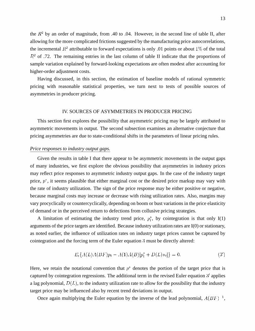
theR2 by an order of magnitude, from .40 to .04. However, in the second line of table II, after

allowing for the more complicated frictions suggested by the manufacturing price autocorrelations,

the incrementalR2 attributable to forward expectations is only .01 points or about1% of the total

R2 of .72. The remaining entries in the last column of table II indicate that the proportions of

sample variation explained by forward-looking expectations are often modest after accounting for

higher-order adjustment costs.

Having discussed, in this section, the estimation of baseline models of rational symmetric

pricing with reasonable statistical properties, we turn next to tests of possible sources of

asymmetries in producer pricing.

IV. SOURCES OF ASYMMETRIES IN PRODUCER PRICING

This section first explores the possibility that asymmetric pricing may be largely attributed to

asymmetric movements in output. The second subsection examines an alternative conjecture that

pricing asymmetries are due to state-conditional shifts in the parameters of linear pricing rules.

Price responses to industry output gaps.

Given the results in table I that there appear to be asymmetric movements in the output gaps

of many industries, we first explore the obvious possibility that asymmetries in industry prices

may reflect price responses to asymmetric industry output gaps. In the case of the industry target

price,p�, it seems plausible that either marginal cost or the desired price markup may vary with

the rate of industry utilization. The sign of the price response may be either positive or negative,

because marginal costs may increase or decrease with rising utilization rates. Also, margins may

vary procyclically or countercyclically, depending on boom or bust variations in the price elasticity

of demand or in the perceived return to defections from collusive pricing strategies.

A limitation of estimating the industry trend price,p�t , by cointegration is that only I(1)

arguments of the price targets are identified. Because industry utilization rates are I(0) or stationary,

as noted earlier, the influence of utilization rates on industry target prices cannot be captured by

cointegration and the forcing term of the Euler equation3 must be directly altered:

EtfA(L)A(BF )pt � A(1)A(B)[p�t +D(L)ut]g = 0: (30)

Here, we retain the notational convention thatp� denotes the portion of the target price that is

captured by cointegration regressions. The additional term in the revised Euler equation30 applies

a lag polynomial,D(L), to the industry utilization rate to allow for the possibility that the industry

target price may be influenced also by recent trend deviations in output.

Once again multiplying the Euler equation by the inverse of the lead polynomial,A(BF )�1,

14

and rearranging gives the revised decision rule

�pt = �A(1)�t�1 + A�(L)�pt�1 + h0�zt�1 + EtfA(1)A(B)A(BF )�1D(L)utg; (9)

= �A(1)�t�1 + A�(L)�pt�1 + h0�zt�1 +D(L)[h0uzt�1]:

Rational forecasts of forward industry utilization rates in the second line of9 are obtained by

applying a restricted coefficient vector,hu, to the information set contained inzt�1.19 For the

equations presented here, four-quarter autoregressions in the industry utilization rates are used

to generate forward utilization forecasts.D(L) is arbitrarily set to a first-order polynomial, the

minimum order that allows us to distinguish between transient price level responses to output

gaps,D(1) = 0, and persistent level responses,D(1) 6= 0.

The first few columns in table III provide several of the key statistics reported in table II, such

as the level and difference decomposition of the factor polynomial,A(L). The statistics may vary

slightly from those in table II because these are the final equations that include either estimated

price responses to output gaps or asymmetric responses to lagged price gaps (discussed in the next

subsection) or both.

Two statistics for utilization rate regressors are reported in table III in the columns headed

by output gap effects. The first is the p-value of a likelihood ratio test for adding the industry

output gap regressors in the RE format required by equation9. A p-value less than .10 indicates a

significant price response to utilization rates. For example, the first line for manufacturing indicates

that manufacturing utilization is a significant determinant of manufacturing prices, with a p-value

of .03. As shown in the remainder of this column, utilization rate forecasts are significant in about

a third of the industries. Generally, this occurs in industries with relatively homogeneous products,

such as textiles (SIC 22) or motor vehicles SIC 371), where an aggregate industry capacity concept

may be more applicable.

The second statistic is the sum of the estimated weights,D(1), on lags of the present-value

of expected utilization rates. The sum of estimated weights for manufacturing is small (and

statistically insignificant), indicating any persistent level effect on industry prices from higher or

lower utilization rates is modest.

The result most relevant for analysis of pricing asymmetries is that the weight sum is positive

for all industries except motor vehicles. This is the traditional sign expected for capacity bottleneck

pressure on industry pricing. However, positive price responses cannot transform negative gap

19The closed-form solution of the coefficient vector for RE forecasts of utilization rates is

hu = A(1)A(B)[�0m H 0][Inm �GH 0]�1(�m �u]

where�u denotes the selector vector forut in zt.

15

asymmetries in outputs into positive gap asymmetries for prices. Thus, output asymmetry is

unlikely to be the source of the positive gap asymmetry noted for industry prices in section II.

Asymmetric pricing due to state-conditional adjustments.

Having taken account of industry price responses to trend deviations in industry output, we

now turn to the nature of price responses to the trend deviations of prices. That is, in contrast to the

usual cyclical analysis of pricing which is geared to output deviations from trend, it seems plausible

that price trend deviations themselves might be a promising indicator of potential asymmetries

in adjustments to price trends. Given direct measurements of price trend deviations, a tractable

analysis is to determine if the roots of the factor polynomials are different when the price is above

trend,�t�1 > 0, or below,�t�1 < 0.

Initial experimentation with the estimated decision rules of all industries indicated that any

detectable switching effect would be confined to a sign split only on the error correction response,

A(1). The intuition for this attractive simplification can be seen by examining the structure of the

error correction decision rule for the two-root case, which is restated here as

�pt = �A(1)�t�1 + A(1)A(B)�1St(�B;�p�): (10)

In contrast to the null hypothesis of symmetric adjustment, the alternative suggested by the results

in table I is that price adjustment speed is slower when the price is above trend. In other words,

when the price gap is positive, the root of the factor polynomial moves towards unity, driving

the error correction response,A(1) � (1 � �), toward zero. However, the remaining term in

equation10 is relatively insensitive to moderate increases in�. First, the present-value summation,

St(:), whose weights sum to one, is unlikely to vary much with moderate increases in the effective

discount rate,�B, which has an upper bound ofB. Second, for discount factors,B, near unity,

the effective coefficient,A(1)=A(B), of the present-value sum is approximately one and also

insensitive to variations in�.

The first two columns in table III under the headingasymmetric price gap effectslist the

p-values of two tests for asymmetric error correction responses of industry prices to signed patterns

of the price gaps. The estimated price response to a positive price gap,�+t�1, is significantly different

from the estimated response to a negative price gap,��t�1, if the p-value in the column headed

by LR(�+t�1; ��

t�1), is .10 or less. This test suggests asymmetric error correction responses are

significant in total manufacturing and in about40% of the SIC two-digit industries. In all cases, the

coefficient of the positive price gap is significantly smaller than the coefficient of the negative price

gap, indicating a positive skew in price adjustments. In fact, the coefficient of the positive price

gap in these industries, shown in the column headed byA+(1), is also not significantly different

16

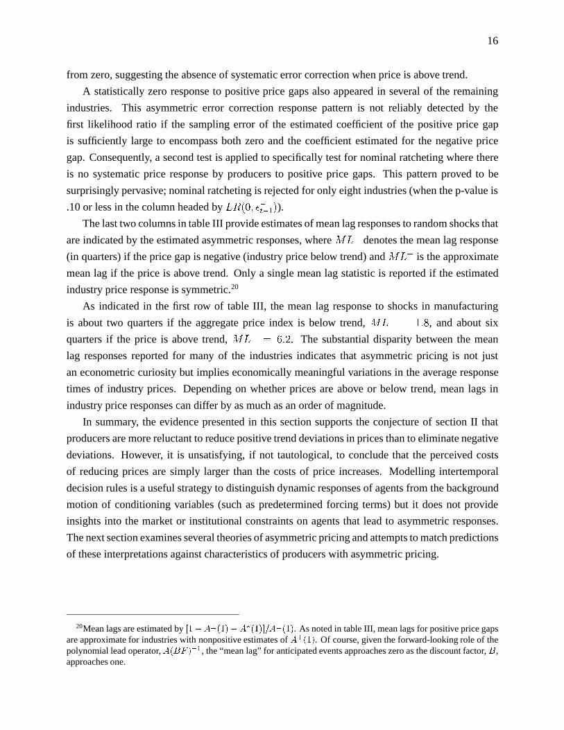
from zero, suggesting the absence of systematic error correction when price is above trend.

A statistically zero response to positive price gaps also appeared in several of the remaining

industries. This asymmetric error correction response pattern is not reliably detected by the

first likelihood ratio if the sampling error of the estimated coefficient of the positive price gap

is sufficiently large to encompass both zero and the coefficient estimated for the negative price

gap. Consequently, a second test is applied to specifically test for nominal ratcheting where there

is no systematic price response by producers to positive price gaps. This pattern proved to be

surprisingly pervasive; nominal ratcheting is rejected for only eight industries (when the p-value is

.10 or less in the column headed byLR(0; ��t�1)).

The last two columns in table III provide estimates of mean lag responses to random shocks that

are indicated by the estimated asymmetric responses, whereML� denotes the mean lag response

(in quarters) if the price gap is negative (industry price below trend) andML+ is the approximate

mean lag if the price is above trend. Only a single mean lag statistic is reported if the estimated

industry price response is symmetric.20

As indicated in the first row of table III, the mean lag response to shocks in manufacturing

is about two quarters if the aggregate price index is below trend,ML� = 1:8, and about six

quarters if the price is above trend,ML+ = 6:2. The substantial disparity between the mean

lag responses reported for many of the industries indicates that asymmetric pricing is not just

an econometric curiosity but implies economically meaningful variations in the average response

times of industry prices. Depending on whether prices are above or below trend, mean lags in

industry price responses can differ by as much as an order of magnitude.

In summary, the evidence presented in this section supports the conjecture of section II that

producers are more reluctant to reduce positive trend deviations in prices than to eliminate negative

deviations. However, it is unsatisfying, if not tautological, to conclude that the perceived costs

of reducing prices are simply larger than the costs of price increases. Modelling intertemporal

decision rules is a useful strategy to distinguish dynamic responses of agents from the background

motion of conditioning variables (such as predetermined forcing terms) but it does not provide

insights into the market or institutional constraints on agents that lead to asymmetric responses.

The next section examines several theories of asymmetric pricing and attempts to match predictions

of these interpretations against characteristics of producers with asymmetric pricing.

20Mean lags are estimated by[1�A�(1)�A�(1)]=A�(1). As noted in table III, mean lags for positive price gapsare approximate for industries with nonpositive estimates ofA+(1). Of course, given the forward-looking role of thepolynomial lead operator,A(BF )�1, the “mean lag” for anticipated events approaches zero as the discount factor,B,approaches one.

17

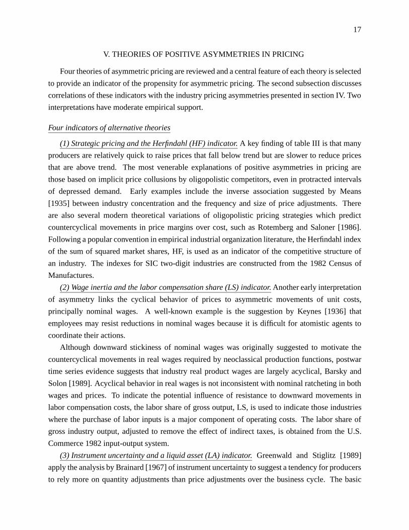
V. THEORIES OF POSITIVE ASYMMETRIES IN PRICING

Four theories of asymmetric pricing are reviewed and a central feature of each theory is selected

to provide an indicator of the propensity for asymmetric pricing. The second subsection discusses

correlations of these indicators with the industry pricing asymmetries presented in section IV. Two

interpretations have moderate empirical support.

Four indicators of alternative theories

(1) Strategic pricing and the Herfindahl (HF) indicator.A key finding of table III is that many

producers are relatively quick to raise prices that fall below trend but are slower to reduce prices

that are above trend. The most venerable explanations of positive asymmetries in pricing are

those based on implicit price collusions by oligopolistic competitors, even in protracted intervals

of depressed demand. Early examples include the inverse association suggested by Means

[1935] between industry concentration and the frequency and size of price adjustments. There

are also several modern theoretical variations of oligopolistic pricing strategies which predict

countercyclical movements in price margins over cost, such as Rotemberg and Saloner [1986].

Following a popular convention in empirical industrial organization literature, the Herfindahl index

of the sum of squared market shares, HF, is used as an indicator of the competitive structure of

an industry. The indexes for SIC two-digit industries are constructed from the 1982 Census of

Manufactures.

(2) Wage inertia and the labor compensation share (LS) indicator.Another early interpretation

of asymmetry links the cyclical behavior of prices to asymmetric movements of unit costs,

principally nominal wages. A well-known example is the suggestion by Keynes [1936] that

employees may resist reductions in nominal wages because it is difficult for atomistic agents to

coordinate their actions.

Although downward stickiness of nominal wages was originally suggested to motivate the

countercyclical movements in real wages required by neoclassical production functions, postwar

time series evidence suggests that industry real product wages are largely acyclical, Barsky and

Solon [1989]. Acyclical behavior in real wages is not inconsistent with nominal ratcheting in both

wages and prices. To indicate the potential influence of resistance to downward movements in

labor compensation costs, the labor share of gross output, LS, is used to indicate those industries

where the purchase of labor inputs is a major component of operating costs. The labor share of

gross industry output, adjusted to remove the effect of indirect taxes, is obtained from the U.S.

Commerce 1982 input-output system.

(3) Instrument uncertainty and a liquid asset (LA) indicator.Greenwald and Stiglitz [1989]

apply the analysis by Brainard [1967] of instrument uncertainty to suggest a tendency for producers

to rely more on quantity adjustments than price adjustments over the business cycle. The basic

18

elements are that producers are risk averse and that price adjustments are perceived to be more

risky than quantity adjustments.

Originally advanced to interpret the (symmetric) inertia of producer prices, this theory can

be modified to explain positive asymmetry in producer prices by adding an asymmetry due to

costs of illiquidity. This altered conjecture has two essential ingredients: (i) the profit variance

associated with price changes is significantly larger than the variance effects of output changes;

and (ii) producer risk varies countercyclically due to imperfect credit markets. Under the first

condition, costs associated with altered production, such as worker hires or layoffs, are relatively

predictable but the profit implications of price changes are more uncertain due to unpredictable

customer or competitor responses.

Under the second condition, risk-neutral firms confronting imperfect credit markets will prefer

self-financing and seek to avoid the costs of bankruptcy or technical insolvency which can trigger

restrictive covenants imposed by creditors. In boom periods with large accumulations of retained

earnings, the probability of exhausting internal liquid asset reserves is small; little weight is

placed on the risk exposure associated with price variations and both price and output are varied

to maximize the discounted stream of expected profits. However, in bad times, self-financing

protection is inevitably eroded by drains on liquid asset buffer stocks, and there is greater concern

about the uncertainty of projected receipts and maintenance of cash flows. Producers become more

cautious about changing prices to alter expected sales and respond to reduced demand prospects

by scaling back the rate of planned production.

The ratio of liquid assets to the capitalized value of earnings, LA, appears to be an appropriate

indicator of a preference for self-financing.21 Note that we are not interested in historical

movements of industry liquid asset ratios but the cross-industry ranking as a guide to the average

self-financing protection selected by industries. Liquid assets are defined as cash and securities

plus inventories less short-term debt; industry data is obtained from the U.S. Department of

Commerce's 1982 Quarterly Financial Report for manufacturing.

(4) Expected inflation and a trend inflation (TI) indicator.The fourth interpretation of

asymmetric pricing is based on the direct costs of changing nominal prices. As outlined in

Tsiddon [1993] and Ball and Mankiw [1994], if menu costs are associated with price changes, a

positive expected drift in the industry price trend will induce asymmetric price responses where

producers are relatively quick to close negative price gaps but slower to reverse positive price

21As in Tinsley [1970a], using a simplifying assumption that earnings in each period are independently distributedand accumulated over a planning horizon, the probability of exhausting liquid asset reserves is exponentially decliningin the ratio of initial reserves to expected earnings divided by the squared coefficient of variation of earnings. Givenimperfect access to credit markets, firms in industries with more volatile earnings will hold higher liquid asset reserves,on average, to met a given probability of technical insolvency. Because equity earnings are highly volatile from periodto period, expected earnings are replaced by the capitalized value of average earnings.

19

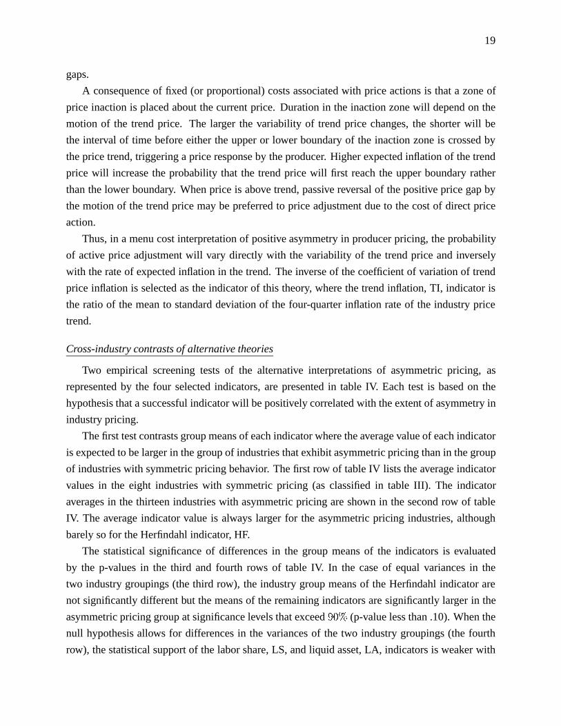
gaps.

A consequence of fixed (or proportional) costs associated with price actions is that a zone of

price inaction is placed about the current price. Duration in the inaction zone will depend on the

motion of the trend price. The larger the variability of trend price changes, the shorter will be

the interval of time before either the upper or lower boundary of the inaction zone is crossed by

the price trend, triggering a price response by the producer. Higher expected inflation of the trend

price will increase the probability that the trend price will first reach the upper boundary rather

than the lower boundary. When price is above trend, passive reversal of the positive price gap by

the motion of the trend price may be preferred to price adjustment due to the cost of direct price

action.

Thus, in a menu cost interpretation of positive asymmetry in producer pricing, the probability

of active price adjustment will vary directly with the variability of the trend price and inversely

with the rate of expected inflation in the trend. The inverse of the coefficient of variation of trend

price inflation is selected as the indicator of this theory, where the trend inflation, TI, indicator is

the ratio of the mean to standard deviation of the four-quarter inflation rate of the industry price

trend.

Cross-industry contrasts of alternative theories

Two empirical screening tests of the alternative interpretations of asymmetric pricing, as

represented by the four selected indicators, are presented in table IV. Each test is based on the

hypothesis that a successful indicator will be positively correlated with the extent of asymmetry in

industry pricing.

The first test contrasts group means of each indicator where the average value of each indicator

is expected to be larger in the group of industries that exhibit asymmetric pricing than in the group

of industries with symmetric pricing behavior. The first row of table IV lists the average indicator

values in the eight industries with symmetric pricing (as classified in table III). The indicator

averages in the thirteen industries with asymmetric pricing are shown in the second row of table

IV. The average indicator value is always larger for the asymmetric pricing industries, although

barely so for the Herfindahl indicator, HF.

The statistical significance of differences in the group means of the indicators is evaluated

by the p-values in the third and fourth rows of table IV. In the case of equal variances in the

two industry groupings (the third row), the industry group means of the Herfindahl indicator are

not significantly different but the means of the remaining indicators are significantly larger in the

asymmetric pricing group at significance levels that exceed90% (p-value less than .10). When the

null hypothesis allows for differences in the variances of the two industry groupings (the fourth

row), the statistical support of the labor share, LS, and liquid asset, LA, indicators is weaker with

20

p-values above .10.

The second set of screening tests in table IV uses regression analysis to estimate the degree

of positive association between indicator values and a measure of the extent of asymmetry in

industry pricing. The sample for the regressions is the cross-section of industries in the group that

exhibited asymmetric pricing. The dependent variable of each cross-section regression is an index

of asymmetric pricing,ML+=ML�, defined as the ratio of the industry mean lag responses to

positive and negative price gaps shown in table III.

The fifth row of table IV displays the bivariate correlations of the asymmetric pricing index

with the relevant industry indicator. The significance of the correlations is indicated by t-ratios in

parentheses. The asymmetric pricing index is most strongly correlated with the liquid asset ratio,

LA, and the trend inflation indicator, TI, where both correlations are moderately strong and have

significance levels well above90%.

The approach in the next row of table IV is to provide an adjustment for possible sampling

errors in the cross-industry indicators. All indicators, except for the trend inflation indicator, TI,

are based on industry values in a given year (1982). On the assumption that the cross-industry

ranks of these indicators are more likely to be invariant to any sampling errors associated with

cardinal measurements drawn from a single year, the industry ranks of the indicators are used as

the relevant regressors in the sixth row of table IV. The major casualty of this adjustment is the

Herfindahl indicator, HF.

Because it is unlikely that there is only a single explanation of asymmetries in industry pricing,

the last two rows of table IV employ multivariate regressions in an attempt to parse the explained

variation in the asymmetric index among competing indicators. The explanatory power of the

multiple indicator regressions is little affected by retaining only the liquid asset indicator, LA,

and the trend inflation indicator, TI, as regressors, as shown in the last row of table IV. The

liquid asset indicator remains statistically significant with a p-value less than .10, whereas the

p-value of the coefficient of the trend inflation indicator is about .15. Bounds on the explanatory

contributions of the indicators can be established by comparing theR2 of the last equation in table

IV with the squares of the simple correlations in the fifth row. This contrast suggests that the liquid

asset indicator, LA, may be explaining from20% to 36% of the total cross-industry variation in

asymmetric pricing, and the trend inflation indicator, TI, may contribute from12% to 28% of the

cross-industry variation.

21

VI. CONCLUDING COMMENTS

This paper provides evidence to support two stylized facts: Production in many manufacturing

industries exhibits negative asymmetry, where shortfalls from trend output are larger, on average,

than positive trend deviations. By contrast, positive asymmetry is more common in producer

pricing where positive trend deviations are more persistent than the deviations of prices below

unit cost trends.

Reasons for these asymmetries in producer responses and the nature of causal interactions

between output and price asymmetries are not resolved in this paper. Although two interpretations,

menu costs and instrument uncertainty, are supported by the simple cross-industry regressions in

the preceding section, this is only suggestive evidence at best. These two candidate theories have

very different implications for interpreting producer behavior and for the design of stabilization

polices.

Under menu costs, expected inflation is a source of asymmetric pricing responses to shocks.

The deadweight loss of inefficient sectoral allocations due to asymmetric price adjustments will

diminish at lower rates of expected inflation. Indeed, if menu costs are symmetric and aggregate

inflation is the sole source of expected drift in industry target prices, this source of asymmetry in

producer pricing will vanish if the expected rate of aggregate inflation is zero.

However, the complication raised in the preceding section is that expected inflation is probably

not the sole cause of asymmetric pricing. Another plausible determinant is instrument uncertainty

where the preferred producer response to unfavorable shocks may be output contraction rather

than price adjustment. If the choice between output or price responses is influenced by the internal

liquidity of firms then the sacrifice ratios of disinflation policies may depend on the cyclical timing

of policy.22 Asymmetric reliance by producers on output responses to reduced demand is also

consistent with concave industry supply functions, where negative output gaps are accompanied

by little or no change in price but output expansions above preferred operating rates may be paired

with large changes in prices. Stabilization polices will increase average output if the supply of

output is a concave function of price.23

Any source of positive price asymmetry may induce negative asymmetries in output, not only

in the same industry through downward sloping demand schedules but also in other industries

through aggregate demand spillover effects of reduced expenditures on material and labor inputs.

However, the instrument uncertainty interpretation suggests that producers respond to unfavorable

22State-conditional aggregate effects of monetary policy are not always cleanly linked with the existence ofstate-dependent producer pricing rules; compare the flexible aggregate price responses in Caplin and Spulber [1987]with the state-dependent real output effects in Caplin and Leahy [1991].

23Denoting the supply of output at a given price byQ(P ), supply is concave inP if Q(:) lies on or below a tangentat the average price,EfPg. It follows, by Jensen's inequality, thatQ(EfPg) � EfQ(P )g.

22

shocks with output adjustmentsin place ofprice responses. This implies that negative output

asymmetry should be matched with positive pricing asymmetry within the same industry. Although

the reductions or reversals of negative asymmetry in the nominal outputs of industries discussed

in section II are suggestive, the possibility of matched asymmetries in price and production (or

employment) decision rules would appear to be a useful topic for future research.

Finally, to underscore the risks of sharp priors on the order of Euler equations, we note that the

empirical models of producer pricing strongly reject the nested specification that price dynamics

are due only to costs of adjusting price levels. The results for both symmetric and asymmetric

responses indicate that the traditional two-root Euler equation description of dynamic pricing

requires ad hoc empirical fixes, including autocorrelated errors and non-rational expectations.

No ad hoc adjustments appear to be necessary if the specification of frictions is relaxed to

accommodate producer incentives to smooth moving averages of prices and rates of inflation.

REFERENCES

Ball, L. and G. Mankiw. “Asymmetric Price Adjustment and Economic Fluctuations.”Economic Journal, 104, March

1994, 247-61.

Barsky, R. and G. Solon. “Real Wages Over the Business Cycle.” NBER Working Paper Series, 2888, March 1989.

Beaulieu, J. and J. Miron. “The Seasonal Cycle in U.S. Manufacturing.” NBER Working Paper Series, 3450, September

1990.

Blinder, A. “Why are Prices Sticky? Preliminary Results From an Interview Study.”American Economic Review, 81(2),

May 1991, 89-96.

Brainard, W. “Uncertainty and the Effectiveness of Policy.”American Economic Review, May 1967, 411-25.

Calvo, G. “Staggered Prices in a Utility-Maximizing Framework.”Journal of Monetary Economics, 12(3), September,

1983, 383-98.

Canova, F. “Detrending and Business Cycle Facts.” CEPR Discussion Paper 782, June 1993.

Caplin, A. and D. Spulber. “Menu Costs and the Neutrality of Money.”Quarterly Journal of Economics, 102, November

1987, 703-26.

Caplin, A. and J. Leahy. “State-Dependent Pricing and the Dynamics of Money and Output.”Quarterly Journal of

Economics, 156(3), August 1991, 683-708.

Carlton, D. “The Rigidity of Prices.”American Economic Review, September 1986, 637-58.

Christiano, L. M. Eichenbaum, and C. Evans. “Identification and the Effects of Monetary Policy Shocks.” Federal

Reserve Bank of Chicago Working Paper 94-7, May 1994.

DeLong, B. and L. Summers. “Are Business Cycles Symmetrical?” inThe American Business Cycle, edited by R.

Gordon. Chicago: The University of Chicago Press, 1986, 166-79.

Falk, B. “Further Evidence on the Asymmetric Behavior of Economic Time Series over the Business Cycle.”Journal of

Political Economy, 94(5), October 1986, 1096-109.

Friedman, M. “The ' Plucking Model' of Business Fluctuations Revisited.”Economic Inquiry, 31, April 1993, 171-7.

23

Goodwin, T. and R. Sweeney. “International Evidence on Friedman's Theory of the Business Cycle.”Economic Inquiry,

31, April 1993, 178-93.

Gonzalo, J. and C. Granger. “Estimation of Common Long-Memory Components in Cointegrated Systems.”Journal of

Business and Economic Statistics, 13(1), January 1995, 27-35.

Greenwald, B. and J. Stiglitz. “Toward a Theory of Rigidities.”American Economic Review, 79, 1989, 364-9.

Haberler, G.Prosperity and Depression. Geneva: League of Nations, 1938.

Harvey, A.Forecasting, Structural Time Series Models, and the Kalman Filter. Cambridge: Cambridge University Press,

1989.

Harvey, A. and A. Jaeger. “Detrending, Stylized Facts, and the Business Cycle.”Journal of Applied Econometrics, 8(3),

July-September 1993, 231-47.

Hicks, J.A Contribution to the Theory of the Trade Cycle. Oxford: Clarendon Press, 1950.

Keynes, J.The General Theory of Employment, Interest and Money. London: Macmillan, 1936.

Lauer, G. and C. Han. “Power of Cochran's Test in the Behrens-Fisher Problem.”Technometrics, 16(4), November

1974, 545-9.

McNevin, B. and S. Neftci. “Some Evidence on the Non-Linearity of Economic Time Series: 1890-1981,” inCycles and

Chaos in Economic Equilibrium, edited by J. Benhabib. Princeton: Princeton University Press, 1991, 429-45.

McQueen, G. and S. Thorley. “Asymmetric Business Cycle Turning Points.”Journal of Monetary Economics, 31, June

1993, 341-62.

Means, G. “Price Inflexibility and the Requirements of a Stabilizing Monetary Policy.”Journal of the American

Statistical Association, 1935, 401-13.

Mitchell, W. Business Cycles. New York: National Bureau of Economic Research, 1927.

Neftci, S. “Are Economic Time Series Asymmetric Over the Business Cycle?”Journal of Political Economy, 92, April

1984, 307-28.

Nelson, C. and H. Kang. “Spurious Periodicity in Inappropriately Detrended Time Series.”Econometrica, 49, 1981,

741-51.

Osborn, D. “Moving Average Detrending of Integrated Processes.” University of Manchester, working paper, March

1993.

Raddock, R. “Revised Federal Reserve Rates of Capacity Utilization.”Federal Reserve Bulletin, 71, October 1985,

754-66.

Rotemberg, J. “Sticky Prices in the United States.”Journal of Political Economy, 90(6), December 1982, 1187- 211.

Rotemberg, J. “The New Keynesian Microfoundations,” inNBER Macroeconomics Annual 1987, edited by S. Fischer.

Cambridge: MIT Press, 1987, 69-104.

Rotemberg, J. and G. Saloner. “A Supergame-Theoretic Model of Price Wars During Booms.”American Economic

Review, 76(3), June, 1986, 390-407.

Sargent, T. “The Ends of Four Big Inflations,” inInflation: Causes and Effects, edited by R. Hall. Chicago: University

of Chicago Press, 1982, 41-97.

Sichel, D. “Business Cycle Asymmetry: A Deeper Look.”Economic Inquiry, 31, April 1993, 224-36.

Sims, C. “Interpreting the Macroeconomic Time Series Facts.”European Economic Review, 36(5), June 1992, 975-

1011.

Swamy, P. and P. Tinsley. “Linear Prediction and Estimation Methods for Regression Models with Stationary Stochastic

24

Coefficients.”Journal of Econometrics, 12(2), February 1980, 103-42.

Taylor, J. “Aggregate Dynamics and Staggered Contracts.”Journal of Political Economy, 88(1), February 1980, 1-23.

Tinsley, P. “Capital Structure, Precautionary Balances, and Valuation of the Firm: The Problem of Financial Risk.”

Journal of Financial and Quantitative Analysis, March 1970(a), 33-61.

Tinsley, P. “On Ramps, Turnpikes, and Distributed Lag Approximations of Optimal Intertemporal Adjustment.”Western

Economic Journal, December 1970(b), 397-411.

Tinsley, P. “Fitting Both Data and Theories: Polynomial Adjustment Costs and Error-Correction Decision Rules.” FRB

FEDS Working Paper 93-21, 1993.

Tobin, J. “Inflation and Unemployment.”American Economic Review, March 1972, 1-18.

Tsiddon, D. “The (Mis)Behavior of the Aggregate Price Level.”Review of Economic Studies, 60(4), October 1993,

889-902.

Waterson, M.Economic Theory of the Industry.Cambridge: Cambridge University Press, 1984.

25

Table I

Asymmetries in Industry Output and Price Trend Deviationsa

ratio of semi-variancesb

growth rates of trend deviations levels of trend deviations

industry SIC real output real output nominal output real output real output nominal output

[OLS trend] [I(1) trend] [I(1) trend] [OLS trend] [I(1) trend] [I(1) trend]

manufacturing 20-39 .47** .50** .67 1.45 .77 .91

food 20 .54*** .55*** 1.19 1.68 .92 3.45

tobacco 21 1.18 .78 1.00 .70* .71 1.24

textiles 22 .82 .95 .76 1.49 .50 .61

apparel 23 .70 .64 .77 .73 .21* .52

lumber 24 .54** .62 .44* .45* .21*** .41*

furniture 25 .54* .48* .44* 1.32 .69 .52*

paper 26 .70 .64 .85 1.49 .41 .77

printing and 27 .76 .72 1.06 1.02 .37* .66publishing

chemicals 28 .63 .55 1.48 1.48 .51* .75

petroleum 29 .66 .70 1.44 1.70 .36* .55refining

rubber and 30 .78 .72 .60 2.20 .53* .60plastics

leather 31 1.33 1.38 .90 .86 .31*** 1.13

stone, clay 32 .86 .73 .92 1.38 .81 .70and glass

primary 33 .48* .67* .60** .93 .41 .48metals

fabricated 34 .54** .50** .65** 1.66 .74 .85metals

nonelectrical 35 .42** .59** .70 .68 .77 1.16machinery

electrical 36 .70 .57** .74 1.28 .64 .75machinery

motor vehicles 371 1.07 1.04 1.11 .60* .36** .34***

other 37x .79 .70 .92 1.85 1.13 2.06transportation

instruments 38 .61* .63* 1.66 .80 .76 2.44

miscellaneous 39 .89 1.10 1.21 1.06 .67 .72

aThe trend in industry log output is represented, alternatively, by the linear trend of log output [OLS trend] and by a

cointegrating trend based on FRB utilization rates [I(1) trend]. Trend deviations in industry nominal output are the sum

of log trend deviations in industry output and price, see text. Sample spans are 1967Q1-1991Q4 for SIC 21, 23, 24, 25,

27, 31, and 39, and 1954Q1-1991Q4 for remaining industries.

bRatio of squared positive mean deviations over squared negative mean deviations. The relevant ratio is less than

unity at 90%(*), 95%(**), and 99%(***) confidence levels; standard errors are corrected for serial correlation using a

Newey-West covariance construction with a bandwidth of� five quarters.

26

Table II

Error Correction Decision Rules for Industry Producer Price Indexesa

�pt = �A(1)�t�1 +A�(L)�pt�1 + S1

t(G;�p�) + at:

adjustment cost price trend(�p�)

parameters expectations

industry SIC lag A(1) A�(1) R2 SEE BG(12) b LR(�p�e) c �R2 d

manufacturing 20-39 1 .10 .40 .0106 .00 .00 .36 (90%)(2.6)

3 .07 .63 .72 .0068 .31 .96 .01 (1%)(2.7) (13.2)

food 20 7 .25 .58 .30 .0311 .61 .13 .00 (0%)(4.6) (3.8)

tobacco 21 2 .18 - .12 .31 .0193 .35 .96 .14 (45%)(3.5) (1.7)

textiles 22 3 .11 .50 .60 .0108 .25 .27 .00 (0%)(4.1) (8.4)

apparel 23 2 .06 .60 .59 .0049 .45 .12 .05 (8%)(1.8) (8.6)

lumber 24 4 .07 .48 .25 .0288 .87 .27 .00 (0%)(1.6) (3.5)

furniture 25 2 .08 .21 .62 .0058 .47 .59 .07 (11%)(2.6) (3.8)

paper 26 2 .13 .60 .62 .0104 .39 .20 .03 (5%)(4.6) (11.2)

printing and 27 2 .11 .50 .65 .0109 .69 .51 .03 (5%)publishing (5.1) (9.4)

chemicals 28 3 .06 .73 .75 .0107 .62 .28 .01 (1%)(3.2) (15.8)

petroleum 29 7 .30 .80 .43 .0552 .11 .24 .05 (12%)refining (5.5) (5.8)

rubber and 30 2 .19 .51 .65 .0090 .56 .20 .08 (12%)plastics (4.9) (9.9)

(Footnotes at end of table)

27

Table II Cont.

Error Correction Decision Rules for Industry Producer Price Indexesa

�pt = �A(1)�t�1 +A�(L)�pt�1 + S1

t (G;�p�) + at:

adjustment cost price trend(�p�)

parameters expectations

industry SIC lag A(1) A�(1) R2 SEE BG(12) b LR(�p�e) c �R2 d

leather 31 5 .08 .29 .38 .0445 .76 .26 .00 (0%)(1.7) (1.6)

stone, clay 32 5 .07 .62 .67 .0081 .31 .70 .03 (4%)and glass (3.4) (9.7)

primary 33 2 .11 .56 .41 .0201 .94 .60 .05 (12%)metals (2.7) (6.3)

fabricated 34 2 .10 .71 .68 .0099 .63 .14 .05 (7%)metals (4.7) (13.9)

nonelectrical 35 5 .08 .61 .83 .0046 .64 .20 .03 (4%)machinery (3.1) (12.4)

electrical 36 4 .08 .27 .75 .0052 .51 .18 .02 (3%)machinery (5.8) (3.6)

motor 371 5 .15 .13 .73 .0089 .90 .37 .00 (0%)vehicles (4.9) (1.2)

other 37x 5 .08 .42 .67 .0076 .60 .24 .06 (9%)transportation (3.9) (4.9)

instruments 38 2 .12 .22 .26 .0181 .98 .56 .03 (12%)(4.0) (2.9)

miscellaneous 39 2 .15 .26 .39 .0138 .18 .96 .07 (18%)(3.6) (3.7)

aSample span 1954Q1 - 1991Q4; t-ratios in parentheses. As in the text,p denotes the log producer price;p� is

the cointegrated price trend;�t is the cointegrating discrepancy,pt � p�t ; andS1

t (G;�p�) is the present-value effect of

anticipated price trend changes.

bBreusch-Godfrey test (p-value) of residual autocorrelation (12 lags).

cLikelihood ratio test (p-value) of RE restrictions on predictions of price trend changes,�p�e.

dChange inR2 due to present-value effect of anticipated price trend changes,S1

t (G;�p�).

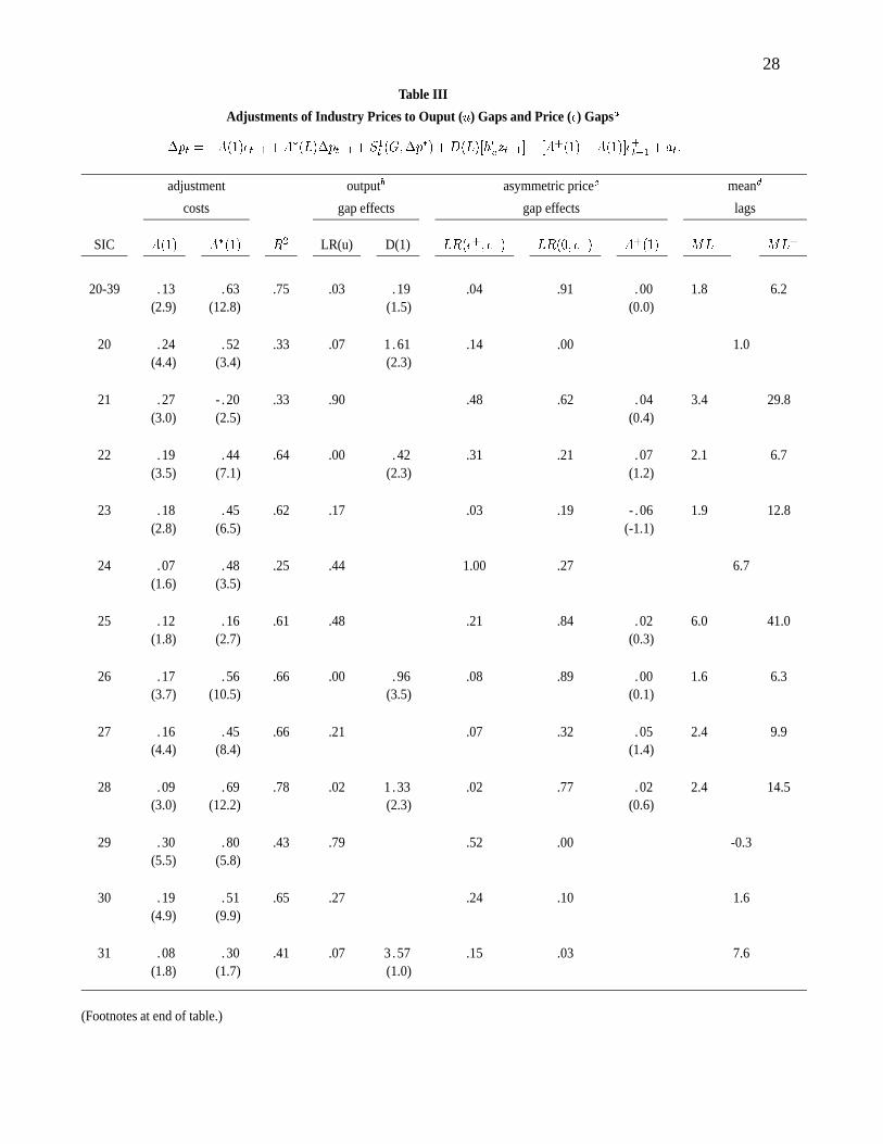
28

Table III

Adjustments of Industry Prices to Ouput (u) Gaps and Price (�) Gapsa

�pt = �A(1)�t�1 +A�(L)�pt�1 + S1t(G;�p�) +D(L)[h0

uzt�1]� [A+(1)�A(1)]�+

t�1+ at:

adjustment outputb asymmetric pricec meand

costs gap effects gap effects lags

SIC A(1) A�(1) R2 LR(u) D(1) LR(�+; ��) LR(0; ��) A+(1) ML� ML+

20-39 .13 .63 .75 .03 .19 .04 .91 .00 1.8 6.2(2.9) (12.8) (1.5) (0.0)

20 .24 .52 .33 .07 1 .61 .14 .00 1.0(4.4) (3.4) (2.3)

21 .27 - .20 .33 .90 .48 .62 .04 3.4 29.8(3.0) (2.5) (0.4)

22 .19 .44 .64 .00 .42 .31 .21 .07 2.1 6.7(3.5) (7.1) (2.3) (1.2)

23 .18 .45 .62 .17 .03 .19 - .06 1.9 12.8(2.8) (6.5) (-1.1)

24 .07 .48 .25 .44 1.00 .27 6.7(1.6) (3.5)

25 .12 .16 .61 .48 .21 .84 .02 6.0 41.0(1.8) (2.7) (0.3)

26 .17 .56 .66 .00 .96 .08 .89 .00 1.6 6.3(3.7) (10.5) (3.5) (0.1)

27 .16 .45 .66 .21 .07 .32 .05 2.4 9.9(4.4) (8.4) (1.4)

28 .09 .69 .78 .02 1 .33 .02 .77 .02 2.4 14.5(3.0) (12.2) (2.3) (0.6)

29 .30 .80 .43 .79 .52 .00 -0.3(5.5) (5.8)

30 .19 .51 .65 .27 .24 .10 1.6(4.9) (9.9)

31 .08 .30 .41 .07 3 .57 .15 .03 7.6(1.8) (1.7) (1.0)

(Footnotes at end of table.)

29

Table III Cont.

Adjustments of Industry Prices to Ouput (u) Gaps and Price (�) Gapsa

�pt = �A(1)�t�1 +A�(L)�pt�1 + S1t(G;�p�) +D(L)[h0

uzt�1]� [A+(1)�A(1)]�+

t�1+ at:

adjustment outputb asymmetric pricec meand

costs gap effects gap effects lags

SIC A(1) A�(1) R2 LR(u) D(1) LR(�+; ��) LR(0; ��) A+(1) ML� ML+

32 .11 .62 .72 .00 .70 .07 .35 .04 2.4 9.3(3.8) (10.2) (3.0) (1.0)

33 .18 .48 .44 .08 .30 .42 .32 .09 1.9 4.9(1.8) (5.1) (1.7) (1.0)

34 .23 .53 .67 .40 .00 .86 .00 1.0 9.6(4.6) (8.9) (0.0)

35 .15 .57 .85 .61 .00 .07 - .06 1.9 11.9(3.5) (12.3) (-1.6)

36 .08 .27 .75 .86 .30 .06 7.7(5.8) (3.6)

371 .16 .01 .75 .02 - .17 .74 .03 5.0(5.3) (0.1) (-2.1)

37x .19 .25 .69 .82 .00 .51 - .00 3.0 29.1(3.9) (2.8) (-0.2)

38 .26 .14 .29 .96 .01 .91 - .01 2.3 15.5(4.0) (1.9) (-0.2)

39 .15 .26 .39 .47 .27 .01 3.9(3.6) (3.7)

aSample span 1954Q1 - 1991Q4; t-ratios in parentheses. As in the text,p denotes the log producer price;p� is the

cointegrated price trend;�t is the price gap,pt � p�t ; �+t and��t denote the positive and negative price gaps.S1t (G;�p�)

is the present-value effect of anticipated price trend changes; andD(L)[h0uzt�1] is the present-value effect of anticipated

output gaps.

bLR(u) is the p-value to accept industry output gap terms,D(L)[h0uzt�1], as significant regressors.

cLR(�+; ��) is the p-value to accept different error-correction responses to the split price gaps,�+ and��; LR(0; ��)

is the p-value to reject a zero error-correction response to positive price gaps,�+.

dMean lag in quarters, conditional on the sign of the price gap. For several industries, the mean lag estimate for

positive price gaps,ML+, is constructed by adding one or two standard errors to nonpositive estimates ofA+(1).

30

Table IV

Proximate Causes of Asymmetric Pricing

industry characteristicsa

herfindahl labor liquid asset trend inflation

index (HF) share (LS) ratio (LA) variation (TI)

industry mean contrastsb

mean of symmetric 754 .24 .21 .59pricing industries

mean of asymmetric 758 .30 .29 .88pricing industries

p-values formean difference:

- equal variances .50 .08 .08 .02

- unequal variances .50 .21 .18 .04

regressions to explain

asymmetric pricing indexc

bivariate correlations:

with industry .45 .14 .60 .53characteristic (1.7) (0.5) (2.5) (2.1)

with rank of industry .23 .22 .54 .53characteristic (0.8) (0.7) (2.1) (2.1)

multivariate regressions:

(R2= :53) .85x10�3 - . 15 9.4 2.7

(0.8) (-0.0) (1.4) (1.3)

(R2= :48) 11.2 2.9

(1.9) (1.5)

aHF - Herfindahl concentration index; LS - employee compensation share of gross output; LA - ratio of net liquid

assets to equity; TI - ratio of mean to standard deviation of four-quarter inflation in industry price trend.

bIndustries exhibiting symmetric or asymmetric pricing as indicated in table III. The p-values are for a one-tail test that

the mean of asymmetric industries exceeds the mean of symmetric industries; p-values for unequal variances are based on

Cochran's test, Lauer and Han [1974].

cDependent variable, defined only for industries exhibiting asymmetric pricing responses, is the ratio of mean lags

shown in table III for positive and negative price gaps,ML+=ML�. Parentheses contain t-ratios.