Radio Science Activities with the ESA-Dresden 1.2 m Ku Band

(10 – 12 GHz) Radio Telescope

Marc CornwallPersonal AssignmentMSc: Space Studies [2007]International Space University (ISU)Advisors: Joachim Köppen, Hugh Hill

Acknowledgements

The author wishes to thank unreservedly:

Prof J. Köppen for his continued technical assistance, with expert and friendly suggestions and advice

Prof H. Hill for his continued logistical assistance and advice

Joel Hermann and Nicolas Moncussi of CNS Lab for assisting with the setup of the ISU EDRT

The “Radio” team for making this a fun filled project

Table of Contents

List of Tables and Figures........................................................................IList of Terms and Acronyms..................................................................IIIWhy Radio Science?...............................................................................1

A Brief History...................................................................................................1Radio Today......................................................................................................2Radio in Education............................................................................................2

The ESA-Dresden Radio Telescope.........................................................3Introduction.......................................................................................................3ISU EDRT Components and Assembly............................................................3

Locating the ISU Outdoor Unit.................................................................................3The Dish Stand.........................................................................................................4Wind Loading and Stability of the IOU.....................................................................4The IOU and the Rotator Units.................................................................................9Configuration of the ISU Indoor Unit and Lightening Safety..................................10

ISU EDRT Calibration.....................................................................................11Positioning Calibration with Satellites.....................................................................11Positioning Accuracy with Astra 1H........................................................................15Noise and Sensitivity with the Sun and Astra 1H...................................................17

Commissioning and Field Observations with the EDRT........................22Catching the Sun.............................................................................................22A Date with the Moon......................................................................................22Charting the Radio Sky...................................................................................23

Lessons Learned from the ISU EDRT....................................................28References...........................................................................................30

List of Tables and Figures

Fig. 1. Reber with his 9.5 m parabolic reflector [RAT]...........................................1Fig. 2. The EDRT Outdoor Unit [Knöchel et al, 20054]..........................................3Fig. 3. The EDRT Indoor Unit [Knöchel et al, 20054].............................................3Fig. 4. Dish Stand showing vertical pole with drilled hole and close-ups of the assembly vertex [Assembly Manual pp. 1 & 5]......................................................4Fig. 5. Diagram illustrating North-South alignment of the IOU...............................4Fig. 6. Concrete Slabs for stability of the Outdoor Unit [Assembly Manual pp. 2 & 6]........................................................................................................................... 5Fig. 7. Windload estimates for the EDRT Fore (collecting) and Aft surfaces.........6Table 1. Windload estimates for the EDRT with reference to the Beaufort scale. .6Fig. 8. Mass Distribution of the ISU EDRT............................................................7Fig. 9. Torque on the ISU EDRT about Dish Stand vertex....................................8Table 2. Torque on the ISU EDRT about Dish Stand vertex with Beaufort reference...............................................................................................................8Fig. 10. Rubber Band wrapped around Mast Clamps [Assembly Manual p. 14]. . .9Fig. 11. Rubber Band anchored to Dish Support Frame [Assembly Manual p. 14].............................................................................................................................. 9Fig. 12. G5500 [Assembly Manual p. 20]..............................................................9Fig. 13. ISU EDRT Architecture...........................................................................10Fig. 14. Custom made junction of the ISU EDRT allowing disconnection of Control Cables.....................................................................................................11Fig. 15. Location of Astra satellites relative to location of EDRT.........................12Fig. 16. The AMA 301 CRT Screen displays the spectrum of Astra 1H..............13Fig. 17. Plot of Satellite Positions, showing the form of the Clarke Belt..............14Fig. 18. Clarke Belt generated by GorbTrack [Walda, 20047]..............................14Fig. 19. Pulsed Elvation Scans Across Astra 1H illustrating lack of symmetry and thus inaccuracy in positioning system [degrees represent actual pointing of the EDRT]..................................................................................................................16Fig. 20. Pulsed Elevation Scans Upward Across Astra 1H, revealing the uncertainty in positioning.....................................................................................17Fig. 21. Contour Plot of the Ku Band radio sky, revealing source free regions of sky.......................................................................................................................18Fig. 22. Plot of observed and modeled system and sky contribution to the received signal....................................................................................................19Fig. 23. Solar Drift Scan from March 16, 2007 at approximately 13:00 local time............................................................................................................................ 20Fig. 24. Solar Flux with Frequency [Generated with Data from Learnmonth Observatory]........................................................................................................20Fig. 25. Solar drift scan of March 16, 2007 [time converted to degrees].............22Fig. 26. Drift scan of the Moon (times shown are local time)...............................23Fig. 27. The Valentine Scan of the ISU EDRT Ku Band radio environment........24Fig. 28. EDRT Ku Band radio environment covering Az 90° – 180° and El 7° – 53°.......................................................................................................................25Fig. 29. Contour image of the ISU radio sky from Az 90° – 180° and El 7° – 53°26

I

Fig. 30. The Clarke Belt Exposed (Astra 1H still stands out)...............................27

II

List of Terms and Acronyms

EDRT – ESA-Dresden Radio TelescopeESA – European Space AgencyLNB – Low Noise BlockAMA 301 – Multifunctional commercial receiver unit of the EDRTRadioAstro – Software package provided with the EDRT to facilitate positioning and signal measurementIOU – ISU Outdoor Unit of the EDRTIIU – ISU Indoor Unit of the EDRTIRO – ISU Radio ObservatoryClarke Belt – Belt of the sky occupied by geostationary satellitesAz – Azimuth, coordinate along the local horizon completing a full 360° circuit starting from 0° in the North.El – Elevation, coordinate concerned with angular distance above the horizon starting from 0° at the horizon up to 90° at the centre of the local sky, the Zenith.EIRP – Effective Isotropic Radiated Power: a power figure used with directional antennas to reference the power which would have to be supplied to an isotropic antenna to generate the same power as the directional antennaHPBW – Half Power Beam Width is the width of the antenna beam 3 dB below the peak sensitivity

III

Why Radio Science?

A Brief History

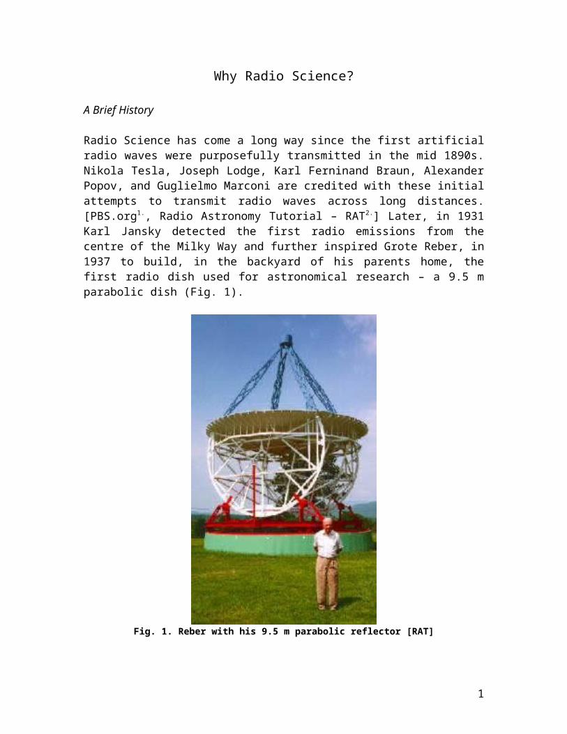
Radio Science has come a long way since the first artificial radio waves were purposefully transmitted in the mid 1890s. Nikola Tesla, Joseph Lodge, Karl Ferninand Braun, Alexander Popov, and Guglielmo Marconi are credited with these initial attempts to transmit radio waves across long distances. [PBS.org1, Radio Astronomy Tutorial – RAT2] Later, in 1931 Karl Jansky detected the first radio emissions from the centre of the Milky Way and further inspired Grote Reber, in 1937 to build, in the backyard of his parents home, the first radio dish used for astronomical research – a 9.5 m parabolic dish (Fig. 1).

Fig. 1. Reber with his 9.5 m parabolic reflector [RAT]

In 1944, Henk Van de Holst, of Holland predicted the existence of the 21 cm hydrogen line, and nearly simultaneously, in 1951, it was detected by 3 teams spread across the globe (Harvard Leiden and Sydney). [Sullivan, 200413]. The 21 cm line occurs in the microwave region of the vast radio atmospheric window, which allows electromagnetic radiation at radio frequencies to arrive at the Earth’s surface. Radio science steadily grew with the detection of the most distant and powerful objects in the Universe Quasars (Quasi-Stellar Radio

1

Sources), and the Cosmic Microwave Background (telling us about the infant Universe) leading up to the discovery of the Pulsar (fast spinning neutron star aiming with radio jets at its poles) by Jocelyn Bell in 1967.

Radio Today

Radio communication is, no doubt, one of the most important aspects of the technological society today. It is used in media broadcasts, exclusively in mobile devices (save for infrared communications) and is indispensable in Space communications technologies. One dare not exclude the importance of Radio Astronomy, which takes astronomers closer to a complete description of the electromagnetic universe. Astronomers are taking it a step further, now with Very Long Baseline Interferometry that synthesizes radio dishes thousands of km in diameter and reveal radio sources, such as massive jets of gas and plasma emanating from the cores of active galaxies, in the finest detail. A continued good understanding of radio phenomena is therefore essential for the uninterrupted functioning of today’s global technological society and a deeper understanding of this vast Universe we live in.

Radio in Education

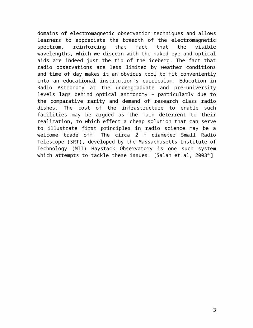
The broad physics and engineering principles which are applicable to radio science makes it an ideal tool for teaching the same in the classroom. It is one of the safer domains of electromagnetic observation techniques and allows learners to appreciate the breadth of the electromagnetic spectrum, reinforcing that fact that the visible wavelengths, which we discern with the naked eye and optical aids are indeed just the tip of the iceberg. The fact that radio observations are less limited by weather conditions and time of day makes it an obvious tool to fit conveniently into an educational institution’s curriculum. Education in Radio Astronomy at the undergraduate and pre-university levels lags behind optical astronomy – particularly due to the comparative rarity and demand of research class radio dishes. The cost of the infrastructure to enable such facilities may be argued as the main deterrent to their realization, to which effect a cheap solution that can serve to illustrate first principles in radio science may be a welcome trade off. The circa 2 m diameter Small Radio Telescope (SRT), developed by the Massachusetts Institute of Technology (MIT) Haystack Observatory is one such system which attempts to tackle these issues. [Salah et al, 20033]

2

The ESA-Dresden Radio Telescope

Introduction

The ESA-Dresden Radio Telescope (EDRT) is a radio receiver system based primarily on commercially available satellite TV equipment. It was developed primarily to address the issues of educational radio astronomy, identified in the previous section, in the interest of the European Space Agency (ESA) and its member states. The system consists of: a 1.2 m offset parabolic reflector with an altazimuth mount and positioning system; a Ku Band (10 – 12 GHz) Low Noise Block (LNB) – Fig. 2 – and a multifunctional commercial receiver (AMA 301) signal reception system; a basic software package to enable positioning and signal measurement from a computer interface (RadioAstro) – Fig. 3. [Knöchel et al, 20054]

Fig. 2. The EDRT Outdoor Unit [Knöchel et al, 20054]

Fig. 3. The EDRT Indoor Unit [Knöchel et al, 20054]

ISU EDRT Components and Assembly

Locating the ISU Outdoor Unit

The ISU Outdoor Unit (IOU) was mounted on the highest platform of the ISU building – i.e. the roof – with, for the most part, an unobstructed view of the entire sky. This was the prime place for a radio installation, as it joined several other satellite receiver dishes previously installed.

3

The Dish Stand

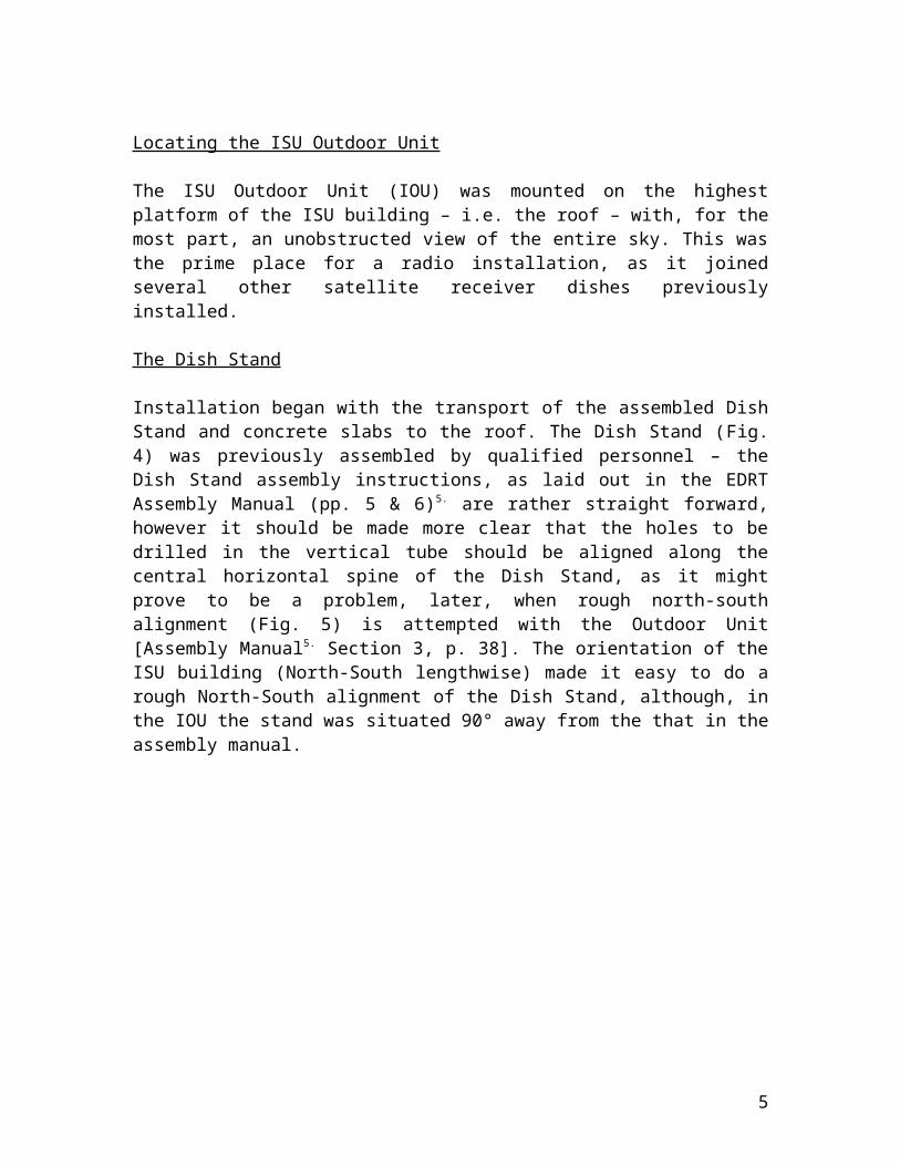
Installation began with the transport of the assembled Dish Stand and concrete slabs to the roof. The Dish Stand (Fig. 4) was previously assembled by qualified personnel – the Dish Stand assembly instructions, as laid out in the EDRT Assembly Manual (pp. 5 & 6)5 are rather straight forward, however it should be made more clear that the holes to be drilled in the vertical tube should be aligned along the central horizontal spine of the Dish Stand, as it might prove to be a problem, later, when rough north-south alignment (Fig. 5) is attempted with the Outdoor Unit [Assembly Manual5 Section 3, p. 38]. The orientation of the ISU building (North-South lengthwise) made it easy to do a rough North-South alignment of the Dish Stand, although, in the IOU the stand was situated 90° away from the that in the assembly manual.

Fig. 4. Dish Stand showing vertical pole with drilled hole and close-ups of the

assembly vertex [Assembly Manual pp. 1 & 5] Fig. 5. Diagram illustrating North-South

alignment of the IOU

Wind Loading and Stability of the IOU

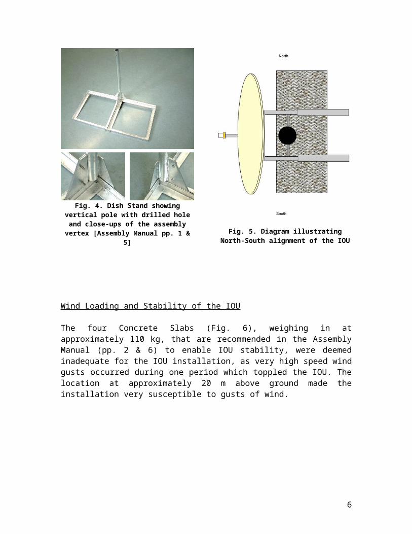
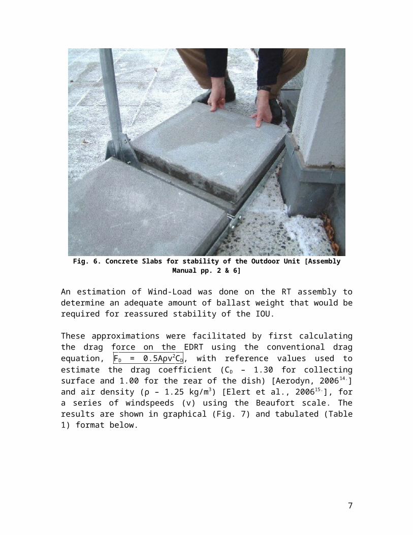
The four Concrete Slabs (Fig. 6), weighing in at approximately 110 kg, that are recommended in the Assembly Manual (pp. 2 & 6) to enable IOU stability, were deemed inadequate for the IOU installation, as very high speed wind gusts occurred during one period which toppled the IOU. The location at approximately 20 m above ground made the installation very susceptible to gusts of wind.

4

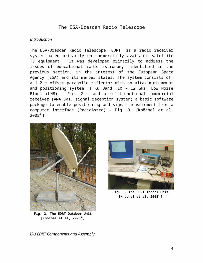
Fig. 6. Concrete Slabs for stability of the Outdoor Unit [Assembly Manual pp. 2 & 6]

An estimation of Wind-Load was done on the RT assembly to determine an adequate amount of ballast weight that would be required for reassured stability of the IOU.

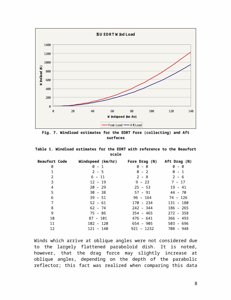
These approximations were facilitated by first calculating the drag force on the EDRT using the conventional drag equation, FD = 0.5Aρv2CD, with reference values used to estimate the drag coefficient (CD – 1.30 for collecting surface and 1.00 for the rear of the dish) [Aerodyn, 200614] and air density (ρ – 1.25 kg/m3) [Elert et al., 200615], for a series of windspeeds (v) using the Beaufort scale. The results are shown in graphical (Fig. 7) and tabulated (Table 1) format below.

5

ISU EDRT Wind Load

0

200

400

600

800

1000

1200

1400

0 20 40 60 80 100 120 140

Windspeed (km/hr)

Win

dloa

d (N

)

Fore Load Aft Load

Fig. 7. Windload estimates for the EDRT Fore (collecting) and Aft surfaces

Table 1. Windload estimates for the EDRT with reference to the Beaufort scale

Beaufort Code Windspeed (km/hr) Fore Drag (N) Aft Drag (N)0 0 – 1 0 – 0 0 – 01 2 – 5 0 – 2 0 – 12 6 – 11 2 – 8 2 – 63 12 – 19 9 – 23 7 – 174 20 – 29 25 – 53 19 – 415 30 – 38 57 – 91 44 – 706 39 – 51 96 – 164 74 – 1267 52 – 61 170 – 234 131 – 1808 62 – 74 242 – 344 186 – 2659 75 – 86 354 – 465 272 – 358

10 87 – 101 476 – 641 366 – 49311 102 – 120 654 – 905 503 – 69612 121 – 140 921 – 1232 708 – 948

Winds which arrive at oblique angles were not considered due to the largely flattened paraboloid dish. It is noted, however, that the drag force may slightly increase at oblique angles, depending on the depth of the parabolic reflector; this fact was realized when comparing this data to that produced in a software tool, ANTWINDTM 11, distributed by Andrew Corporation. The windload generated by ANTWINDTM for an analogous setup was similar but approximately 1.39 times greater in magnitude. This is thought to be due to the greater depth in the parabolic reflector model used by the software.

6

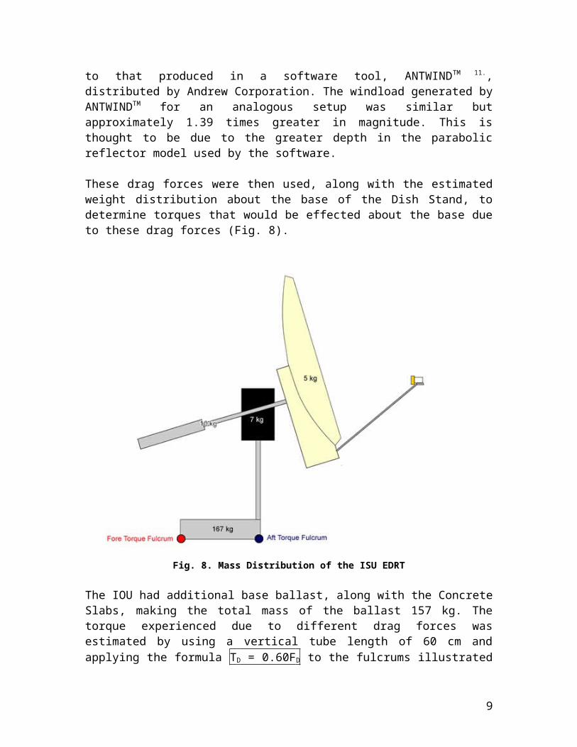
These drag forces were then used, along with the estimated weight distribution about the base of the Dish Stand, to determine torques that would be effected about the base due to these drag forces (Fig. 8).

Fig. 8. Mass Distribution of the ISU EDRT

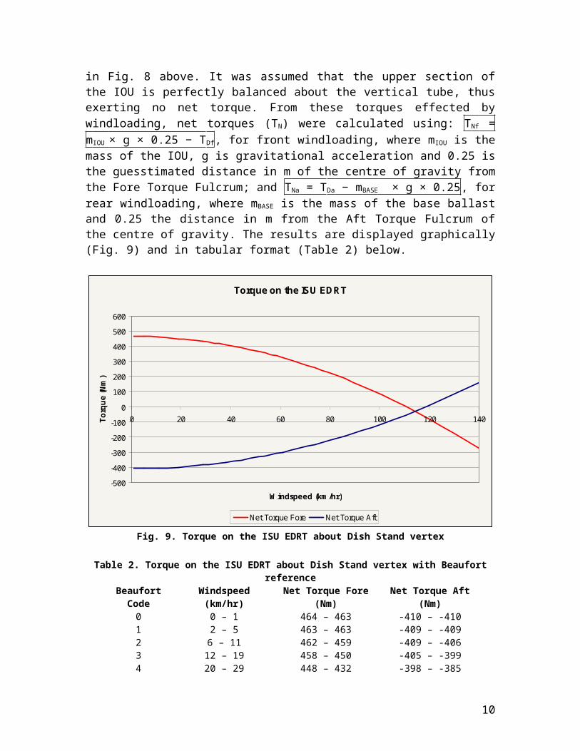
The IOU had additional base ballast, along with the Concrete Slabs, making the total mass of the ballast 157 kg. The torque experienced due to different drag forces was estimated by using a vertical tube length of 60 cm and applying the formula TD = 0.60FD to the fulcrums illustrated in Fig. 8 above. It was assumed that the upper section of the IOU is perfectly balanced about the vertical tube, thus exerting no net torque. From these torques effected by windloading, net torques (TN) were calculated using: TNf = mIOU × g × 0.25 − TDf, for front windloading, where mIOU is the mass of the IOU, g is gravitational acceleration and 0.25 is the guesstimated distance in m of the centre of gravity from the Fore Torque Fulcrum; and TNa = TDa − mBASE × g × 0.25, for rear windloading, where mBASE is the mass of the base ballast and 0.25 the distance in m from the Aft Torque Fulcrum of the centre of gravity. The results are displayed graphically (Fig. 9) and in tabular format (Table 2) below.

7

Torque on the ISU EDRT

-500

-400

-300

-200

-100

0

100

200

300

400

500

600

0 20 40 60 80 100 120 140

Windspeed (km/hr)

Torq

ue (N

m)

Net Torque Fore Net Torque Aft

Fig. 9. Torque on the ISU EDRT about Dish Stand vertex

Table 2. Torque on the ISU EDRT about Dish Stand vertex with Beaufort referenceBeaufort Code Windspeed (km/hr) Net Torque Fore (Nm) Net Torque Aft (Nm)

0 0 – 1 464 – 463 -410 – -4101 2 – 5 463 – 463 -409 – -4092 6 – 11 462 – 459 -409 – -4063 12 – 19 458 – 450 -405 – -3994 20 – 29 448 – 432 -398 – -3855 30 – 38 430 – 409 -383 – -3686 39 – 51 406 – 365 -365 – -3347 52 – 61 362 – 323 -331 – -3028 62 – 74 319 – 257 -298 – -2519 75 – 86 251 – 185 -246 – -195

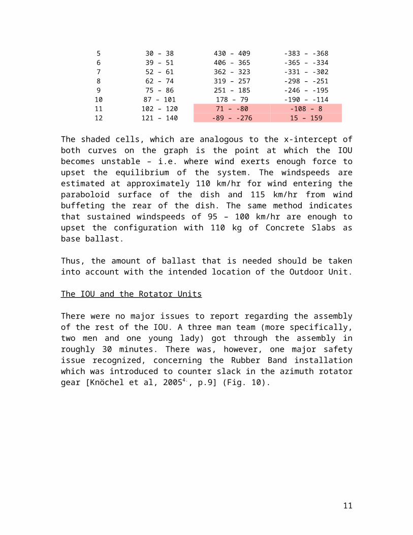
10 87 – 101 178 – 79 -190 – -11411 102 – 120 71 – -80 -108 – 812 121 – 140 -89 – -276 15 – 159

The shaded cells, which are analogous to the x-intercept of both curves on the graph is the point at which the IOU becomes unstable – i.e. where wind exerts enough force to upset the equilibrium of the system. The windspeeds are estimated at approximately 110 km/hr for wind entering the paraboloid surface of the dish and 115 km/hr from wind buffeting the rear of the dish. The same method indicates that sustained windspeeds of 95 – 100 km/hr are enough to upset the configuration with 110 kg of Concrete Slabs as base ballast.

Thus, the amount of ballast that is needed should be taken into account with the intended location of the Outdoor Unit.

8

The IOU and the Rotator Units

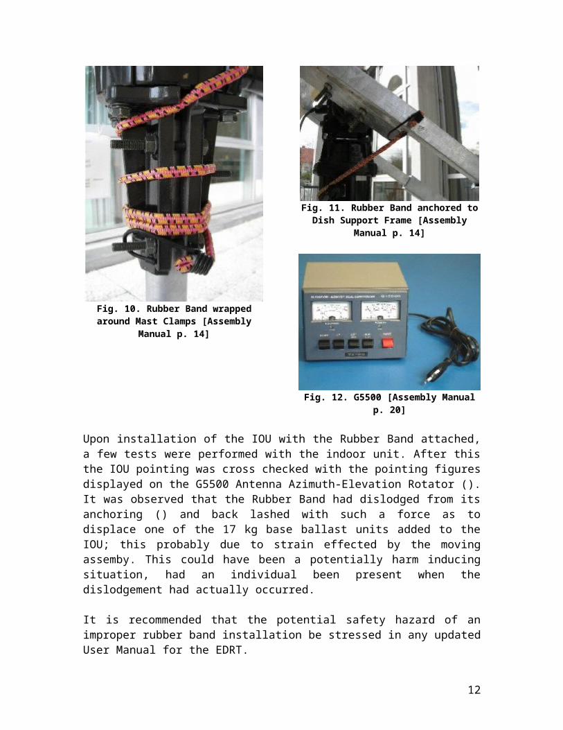
There were no major issues to report regarding the assembly of the rest of the IOU. A three man team (more specifically, two men and one young lady) got through the assembly in roughly 30 minutes. There was, however, one major safety issue recognized, concerning the Rubber Band installation which was introduced to counter slack in the azimuth rotator gear [Knöchel et al, 20054, p.9] (Fig. 10).

Fig. 10. Rubber Band wrapped around Mast Clamps [Assembly Manual p. 14]

Fig. 11. Rubber Band anchored to Dish Support Frame [Assembly Manual p. 14]

Fig. 12. G5500 [Assembly Manual p. 20]

Upon installation of the IOU with the Rubber Band attached, a few tests were performed with the indoor unit. After this the IOU pointing was cross checked with the pointing figures displayed on the G5500 Antenna Azimuth-Elevation Rotator (). It was observed that the Rubber Band had dislodged from its anchoring () and back lashed with such a force as to displace one of the 17 kg base ballast units added to the IOU; this probably due to strain effected by the moving assemby. This could have been a potentially harm inducing situation, had an individual been present when the dislodgement had actually occurred.

It is recommended that the potential safety hazard of an improper rubber band installation be stressed in any updated User Manual for the EDRT.

9

Configuration of the ISU Indoor Unit and Lightening Safety

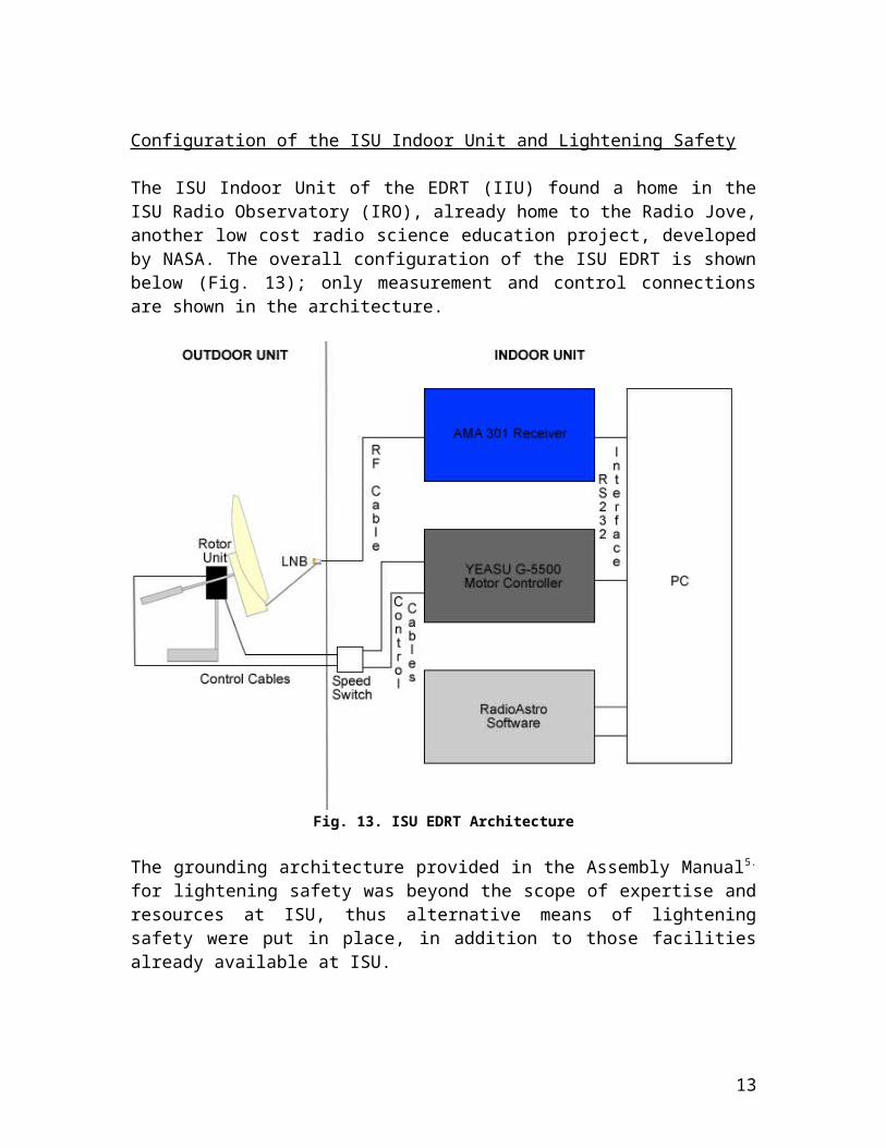
The ISU Indoor Unit of the EDRT (IIU) found a home in the ISU Radio Observatory (IRO), already home to the Radio Jove, another low cost radio science education project, developed by NASA. The overall configuration of the ISU EDRT is shown below (Fig. 13); only measurement and control connections are shown in the architecture.

Fig. 13. ISU EDRT Architecture

The grounding architecture provided in the Assembly Manual5 for lightening safety was beyond the scope of expertise and resources at ISU, thus alternative means of lightening safety were put in place, in addition to those facilities already available at ISU.

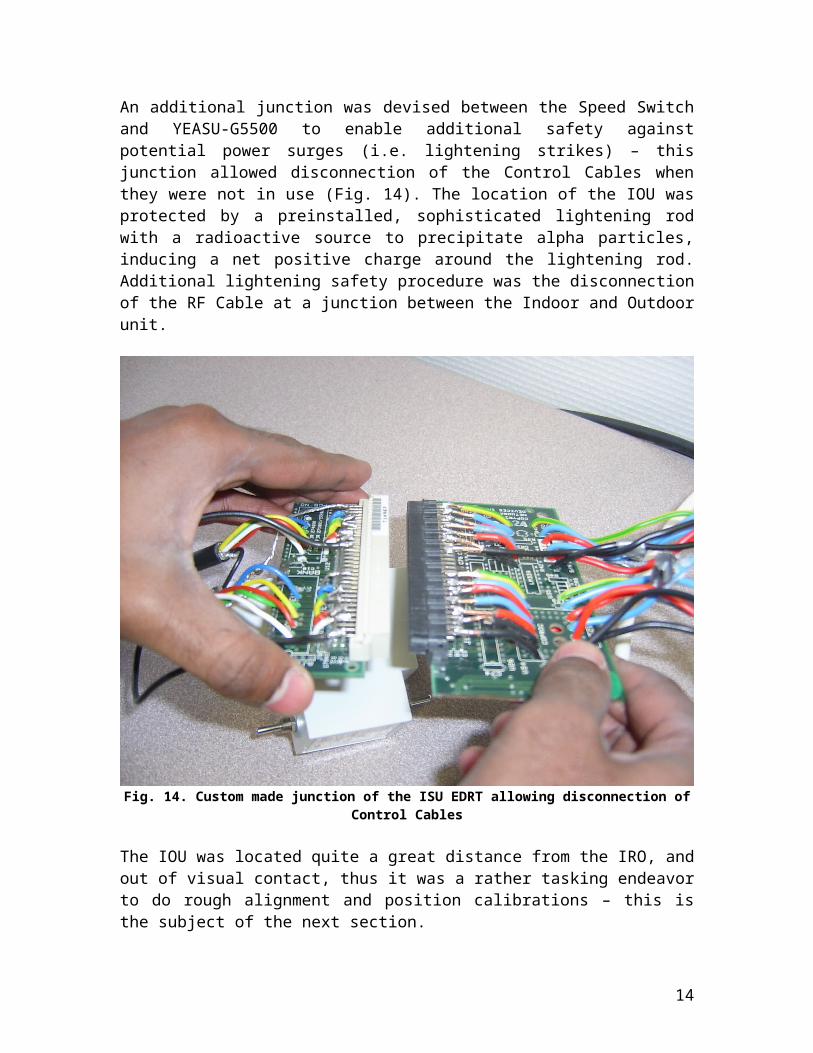
An additional junction was devised between the Speed Switch and YEASU-G5500 to enable additional safety against potential power surges (i.e. lightening strikes) – this junction allowed disconnection of the Control Cables when they were not in use (Fig. 14). The location of the IOU was protected by a preinstalled, sophisticated lightening rod with a radioactive source to precipitate alpha particles, inducing a net positive charge around the lightening rod. Additional

10

lightening safety procedure was the disconnection of the RF Cable at a junction between the Indoor and Outdoor unit.

Fig. 14. Custom made junction of the ISU EDRT allowing disconnection of Control Cables

The IOU was located quite a great distance from the IRO, and out of visual contact, thus it was a rather tasking endeavor to do rough alignment and position calibrations – this is the subject of the next section.

ISU EDRT Calibration

Unless otherwise stated, all radio measurements are taken at the frequency of 12500 MHz at horizontal polarization.

Positioning Calibration with Satellites

The positioning system comprises potentiometers located in the Rotator Unit and YEASU-G5500 Control Unit. The potentiometers in the Rotator Unit have a voltage corresponding to a particular angular position of the motors; similarly the YEASU-G5500 potentiometers associate a particular voltage received from the control cables to an angular deflection of the Azimuth (Az) or Elevation (El) dial. As will be seen later in the Commissioning and Field Observations section, this

11

potentiometer setup served to be a source of active deviations in the position reading.

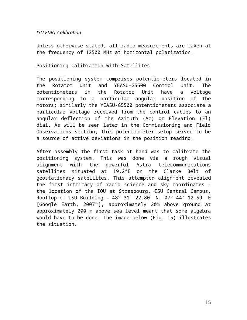
After assembly the first task at hand was to calibrate the positioning system. This was done via a rough visual alignment with the powerful Astra telecommunications satellites situated at 19.2°E on the Clarke Belt of geostationary satellites. This attempted alignment revealed the first intricacy of radio science and sky coordinates – the location of the IOU at Strasbourg, ISU Central Campus, Rooftop of ISU Building – 48° 31’ 22.80” N, 07° 44’ 12.59” E [Google Earth, 20076], approximately 20m above ground at approximately 200 m above sea level meant that some algebra would have to be done. The image below (Fig. 15) illustrates the situation.

Fig. 15. Location of Astra satellites relative to location of EDRT

The image shows that while the Astra satellites are displaced 19.2°E of 0° on the Clarke Belt, which corresponds to 0° longitude on Earth, the location from the EDRT, East of 180° in the EDRT sky is actually 19.2 – 7.75, i.e. 11.45°E or 168.55° Az. One may make the mistake of looking for the satellite at 19.2° East of 180° along the horizon (161.8° Az).

After the rough alignment the strong satellite signal was found with some trial and error. The analogue dials on the G5500 were very hard to read accurately (± 7° absolute accuracy). A digital readout was favorable and thus the RadioAstro software was employed to see the position at the precision of 1°.

Telecommunications satellites can be easily identified via the narrow bandwidth spikes that their individual transponders produce on a radio spectrum. The CRT video screen of the AMA 301 proved invaluable in this respect as the distinctive profile of a different satellite was immediately recognizable due to the occupations of different frequencies by the transponders on each satellite, to avoid electromagnetic interference. Attempts were made to identify satellites by

12

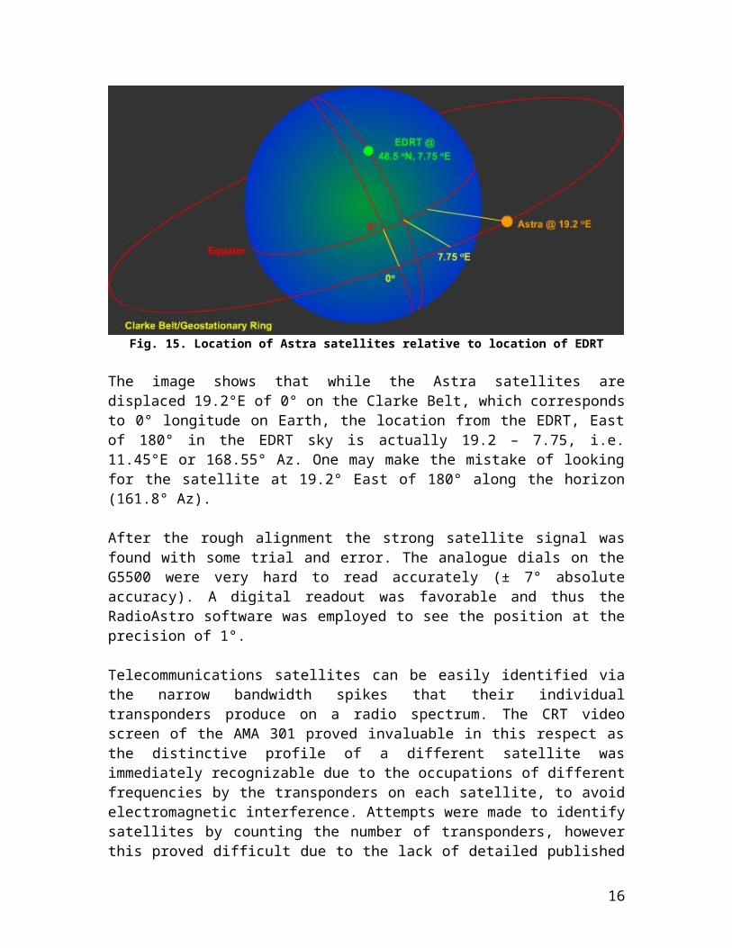
counting the number of transponders, however this proved difficult due to the lack of detailed published data on these technical characteristics; the spectrum of the Astra 1H satellite as displayed by the AMA 301 is shown below (Fig. 16).

Fig. 16. The AMA 301 CRT Screen displays the spectrum of Astra 1H

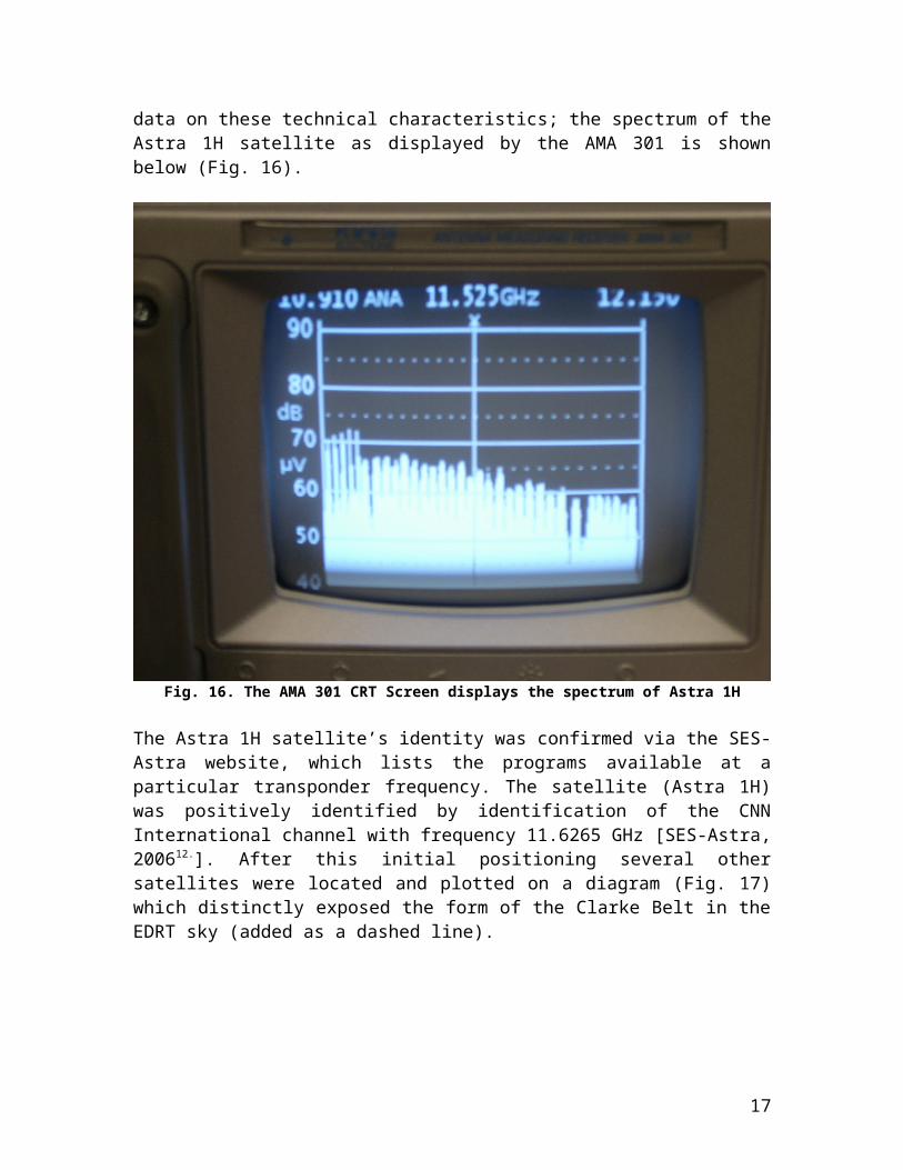
The Astra 1H satellite’s identity was confirmed via the SES-Astra website, which lists the programs available at a particular transponder frequency. The satellite (Astra 1H) was positively identified by identification of the CNN International channel with frequency 11.6265 GHz [SES-Astra, 200612]. After this initial positioning several other satellites were located and plotted on a diagram (Fig.17) which distinctly exposed the form of the Clarke Belt in the EDRT sky (added as a dashed line).

13

Clarke Belt

153, 29

128, 17

147, 27

121, 14

184, 34

207, 30

224, 24

237, 16

168, 33

0

5

10

15

20

25

30

35

40

90 100 110 120 130 140 150 160 170 180 190 200 210 220 230 240 250 260 270

Azimuth

Elev

atio

n

Fig. 17. Plot of Satellite Positions, showing the form of the Clarke Belt

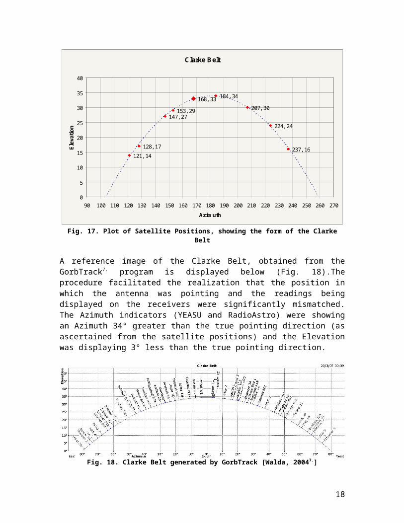
A reference image of the Clarke Belt, obtained from the GorbTrack7 program is displayed below (Fig. 18).The procedure facilitated the realization that the position in which the antenna was pointing and the readings being displayed on the receivers were significantly mismatched. The Azimuth indicators (YEASU and RadioAstro) were showing an Azimuth 34° greater than the true pointing direction (as ascertained from the satellite positions) and the Elevation was displaying 3° less than the true pointing direction.

Fig. 18. Clarke Belt generated by GorbTrack [Walda, 20047]

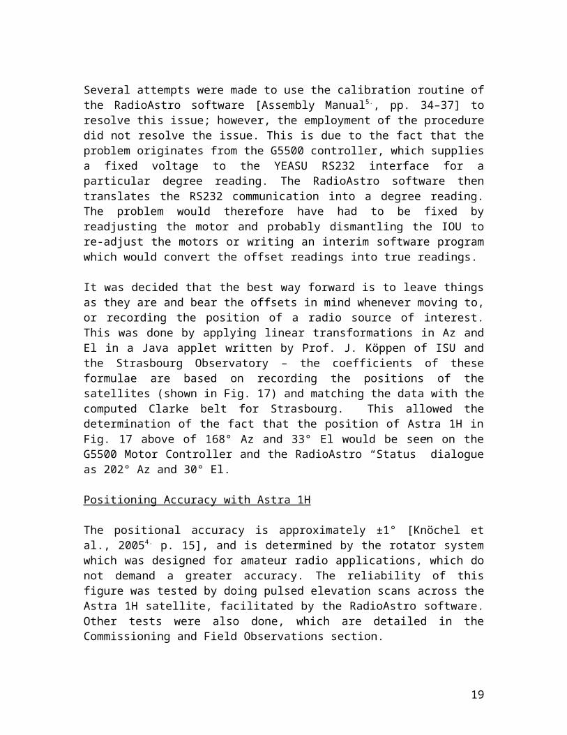
Several attempts were made to use the calibration routine of the RadioAstro software [Assembly Manual5, pp. 34–37] to resolve this issue; however, the employment of the procedure did not resolve the issue. This is due to the fact that the problem originates from the G5500 controller, which supplies a fixed voltage to the YEASU RS232 interface for a particular degree reading. The

14

RadioAstro software then translates the RS232 communication into a degree reading. The problem would therefore have had to be fixed by readjusting the motor and probably dismantling the IOU to re-adjust the motors or writing an interim software program which would convert the offset readings into true readings.

It was decided that the best way forward is to leave things as they are and bear the offsets in mind whenever moving to, or recording the position of a radio source of interest. This was done by applying linear transformations in Az and El in a Java applet written by Prof. J. Köppen of ISU and the Strasbourg Observatory – the coefficients of these formulae are based on recording the positions of the satellites (shown in Fig. 17) and matching the data with the computed Clarke belt for Strasbourg. This allowed the determination of the fact that the position of Astra 1H in Fig. 17 above of 168° Az and 33° El would be seen on the G5500 Motor Controller and the RadioAstro “Status” dialogue as 202° Az and 30° El.

Positioning Accuracy with Astra 1H

The positional accuracy is approximately ±1° [Knöchel et al., 20054 p. 15], and is determined by the rotator system which was designed for amateur radio applications, which do not demand a greater accuracy. The reliability of this figure was tested by doing pulsed elevation scans across the Astra 1H satellite, facilitated by the RadioAstro software. Other tests were also done, which are detailed in the Commissioning and Field Observations section.

RadioAstro is a basic astronomy software that allows the positioning of the the EDRT with resolution of 1°. It has the limitation that it cannot go below El 5°, which would have been a rather useful feature for the purposes of antenna temperature calibration using the ambient temperature of the ground. The software also facilitates near real-time measurement, recording and storage of power values using a basic signal processing and plotting software. The pulsed feature which RadioAstro sports allows the speed of the Az and El motors to be changed independently, thus facilitating tracking of astronomical radio sources.

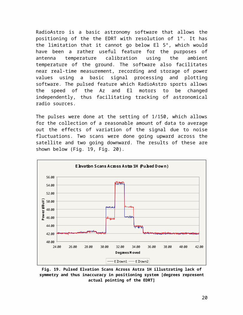
The pulses were done at the setting of 1/150, which allows for the collection of a reasonable amount of data to average out the effects of variation of the signal due to noise fluctuations. Two scans were done going upward across the satellite and two going downward. The results of these are shown below (Fig. 19, Fig.20).

15

Elevation Scans Across Astra 1H (Pulsed Down)

40.00

42.00

44.00

46.00

48.00

50.00

52.00

54.00

56.00

24.00 26.00 28.00 30.00 32.00 34.00 36.00 38.00 40.00 42.00

Degrees Moved

Pow

er (d

BuV)

ElDown1 ElDown2

Fig. 19. Pulsed Elvation Scans Across Astra 1H illustrating lack of symmetry and thus inaccuracy in positioning system [degrees represent actual pointing of the EDRT]

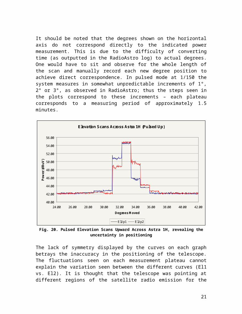
It should be noted that the degrees shown on the horizontal axis do not correspond directly to the indicated power measurement. This is due to the difficulty of converting time (as outputted in the RadioAstro log) to actual degrees. One would have to sit and observe for the whole length of the scan and manually record each new degree position to achieve direct correspondence. In pulsed mode at 1/150 the system measures in somewhat unpredictable increments of 1°, 2° or 3°, as observed in RadioAstro; thus the steps seen in the plots correspond to these increments – each plateau corresponds to a measuring period of approximately 1.5 minutes.

16

Elevation Scans Across Astra 1H (Pulsed Up)

40.00

42.00

44.00

46.00

48.00

50.00

52.00

54.00

56.00

24.00 26.00 28.00 30.00 32.00 34.00 36.00 38.00 40.00 42.00

Degrees Moved

Pow

er (d

BuV)

ElUp1 ElUp2

Fig. 20. Pulsed Elevation Scans Upward Across Astra 1H, revealing the uncertainty in positioning

The lack of symmetry displayed by the curves on each graph betrays the inaccuracy in the positioning of the telescope. The fluctuations seen on each measurement plateau cannot explain the variation seen between the different curves (El1 vs. El2). It is thought that the telescope was pointing at different regions of the satellite radio emission for the two scans, hence the difference in recorded power level for the same degree (or time) reading. It can be seen that this inaccuracy is of the order 1°, 2° or 3° as observed in the pulsed increments displayed in the RadioAstro status dialogue.

Noise and Sensitivity with the Sun and Astra 1H

It was noticed that the noise background of the sky increased with decreasing El as illustrated in sky scan images discussed later (Fig. 27). Characterizing and minimizing the noise environment is an important aspect of radio science due to the fact that source variation and random noise variations need to be separated to determine the true flux from the source. To this effect several elevation scans were done, one use of which would be to model a relationship for the noise contribution of the sky background and the receiver system. Scans where the sky was free of significant radio sources were averaged, and a model was used to extract approximate values for the noise contribution of the receiving system and the sky background. This model states that the receiver power (PR) is given by PR (dBµV) = 10log10 [10[(PR)/10] + (10(PSKY/10))cosec(El)]. PR represents the noise background from the receiver and LNB and PSKY the sky background.

17

As there were many scan samples, and it would be tedious to analyze them singly to isolate the most suitable ones, they were converted to a 2D matrix of the Ku Band power values along the Azimuth and Elevation of the sky and plotted on a contour (Fig. 21), generated by Matlab, to reveal the source free regions. It is worthy to note that there was sometimes a 1° variation in the position readings during these scans, where, for a scan in elevation, the Az value started at is 1° less than the value the scan ends on. This was determined to be due to the YEASU-G5500 motor controller warming up, as after prolonged use, the figures remained constant.

Fig. 21. Contour Plot of the Ku Band radio sky, revealing source free regions of sky

It is clear that the regions around Az 110° (20 on the plot) and Az 130° – 140° (40 – 50 on the plot) are source free and should be prime candidates for modeling the sky and LNB contribution to the noise background. The Clarke Belt GEO satellites can be seen rising from Az 120° up towards El 28° at the right end of the plot. The streaks along elevation towards Az 90° represent elevated noise levels and are thought to be due to weather conditions, it is surmised that high humidity and cloud conditions contributed to the observed anomalies as it was positively observed on one occasion that cloudy, humid weather coincided with the times these scans were taken. Additionally, a Holiday Inn hotel is located close to Az 90° at low elevations, and may be the source of the elevated radio emission observed there.

18

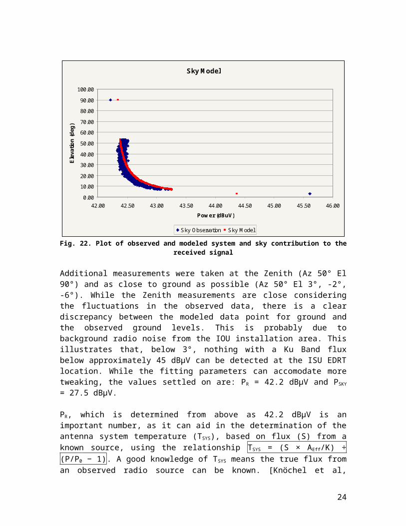
The plot of the radio background with elevation is shown below (Fig. 22).

Sky Model

0.00

10.00

20.00

30.00

40.00

50.00

60.00

70.00

80.00

90.00

100.00

42.00 42.50 43.00 43.50 44.00 44.50 45.00 45.50 46.00

Power (dBuV)

Elev

atio

n (d

eg)

Sky Observation Sky Model

Fig. 22. Plot of observed and modeled system and sky contribution to the received signal

Additional measurements were taken at the Zenith (Az 50° El 90°) and as close to ground as possible (Az 50° El 3°, -2°, -6°). While the Zenith measurements are close considering the fluctuations in the observed data, there is a clear discrepancy between the modeled data point for ground and the observed ground levels. This is probably due to background radio noise from the IOU installation area. This illustrates that, below 3°, nothing with a Ku Band flux below approximately 45 dBµV can be detected at the ISU EDRT location. While the fitting parameters can accomodate more tweaking, the values settled on are: PR

= 42.2 dBµV and PSKY = 27.5 dBµV.

PR, which is determined from above as 42.2 dBµV is an important number, as it can aid in the determination of the antenna system temperature (TSYS), based on flux (S) from a known source, using the relationship TSYS = (S × AEff/K) ÷ (P/P0 − 1). A good knowledge of TSYS means the true flux from an observed radio source can be known. [Knöchel et al, 20058] The Sun was used to determine TSYS for the EDRT. AEff is taken from Knöchel et al8 as 0.842546 m2. Data is used from an EDRT Solar Drift Scan dated March 16, 2007 with maximum pass estimated at 12:26:01 Universal Time – UT (Fig. 23). The maximum is taken as 49.5 dBµV.

19

Solar Flux

41.0

42.0

43.0

44.0

45.0

46.0

47.0

48.0

49.0

50.0

13:0

1:29

13:0

3:51

13:0

6:13

13:0

8:35

13:1

0:57

13:1

3:19

13:1

5:41

13:1

8:03

13:2

0:26

13:2

2:48

13:2

5:10

13:2

7:32

13:2

9:54

13:3

2:17

13:3

4:39

13:3

7:01

13:3

9:23

13:4

1:45

13:4

4:07

13:4

6:29

13:4

8:51

13:5

1:14

13:5

3:36

13:5

5:58

13:5

8:20

14:0

0:42

Time (HH:MM:SS)

Pow

er (d

BuV)

Fig. 23. Solar Drift Scan from March 16, 2007 at approximately 13:00 local time

Reference data for the solar flux from that period was obtained from the IPS of the Learnmonth Observatory (http://www.ips.gov.au/Solar/3/4/2) for the date of March 21, 2007 as earlier data could not be accessed. The solar flux at 12.5 GHz was obtained from the observed and calculated data sets available via a graphical plot (Fig. 24).

Solar Flux wtih Frequency

0

100

200

300

400

500

600

200 2200 4200 6200 8200 10200 12200 14200

Frequency (MHz)

Flux

(sfu

)

Fig. 24. Solar Flux with Frequency [Generated with Data from Learnmonth Observatory]

The solar flux is estimated at 360 sfu (3.6×10 -20 Wm-2Hz-1), which corresponds to a TSYS of 503 K. The gain used in the Calibration Report of Knöchel et al8 was

20

used to obtain a G/T ratio of 0.09 dBi/K. The fact that the solar flux used is not for the exact day means this calculation should be taken with caution, particularly that uncertainty in solar flux contributes significantly to the uncertainty in determining TSYS; however, it demonstrates the methodology quite well.

With the determination of TSYS the received power from a source, as indicated on the receiver, can then be translated into the actual flux from the source – this is tried with the Astra 1H satellite. The plots in Fig. 19 and Fig. 20 are used as reference values where the maximum power of the satellite (P) is taken to be 55 dBµV and the noise background (P0) as 42.2 dBµV. With this the power flux of the Astra 1H satellite is calculated – with rearrangement of the TSYS relationship for flux – to be 5.19 nWm-2Hz-1.

Official SES-Astra documentation lists the Effective Isotropic Radiated Power (EIRP) of the Astra 1H transmit antenna as 51 dBW [SES-Astra, 20069]. Converted to power in watts the Astra 1H transmits at a power of 126 kW [Radio Spectrum Management10]. As the power density will decrease with distance, the power at the distance of the EDRT, which is 42,169.7 km according to GorbTrack7 (the earth radius of 6378 km was subtracted), is PAstra1H ÷ 4π × (DAstra1H)2. Thus, the power (SAstra1H) incident on a unit surface area of the EDRT Dish is expected to be 7.82 pWm-2Hz-1.

The source and nature of the discrepancies in the values determined is unclear – in any event both seem to be largely over estimated. One possible cause in the latter analysis might be that free space loss was not taken into account, as well at the fact that an EIRP value of 51 dBW is a maximum value and will vary depending on where exactly in the satellite footprint the receiving station is located. This issue is still being investigated.

21

Commissioning and Field Observations with the EDRT

Catching the Sun

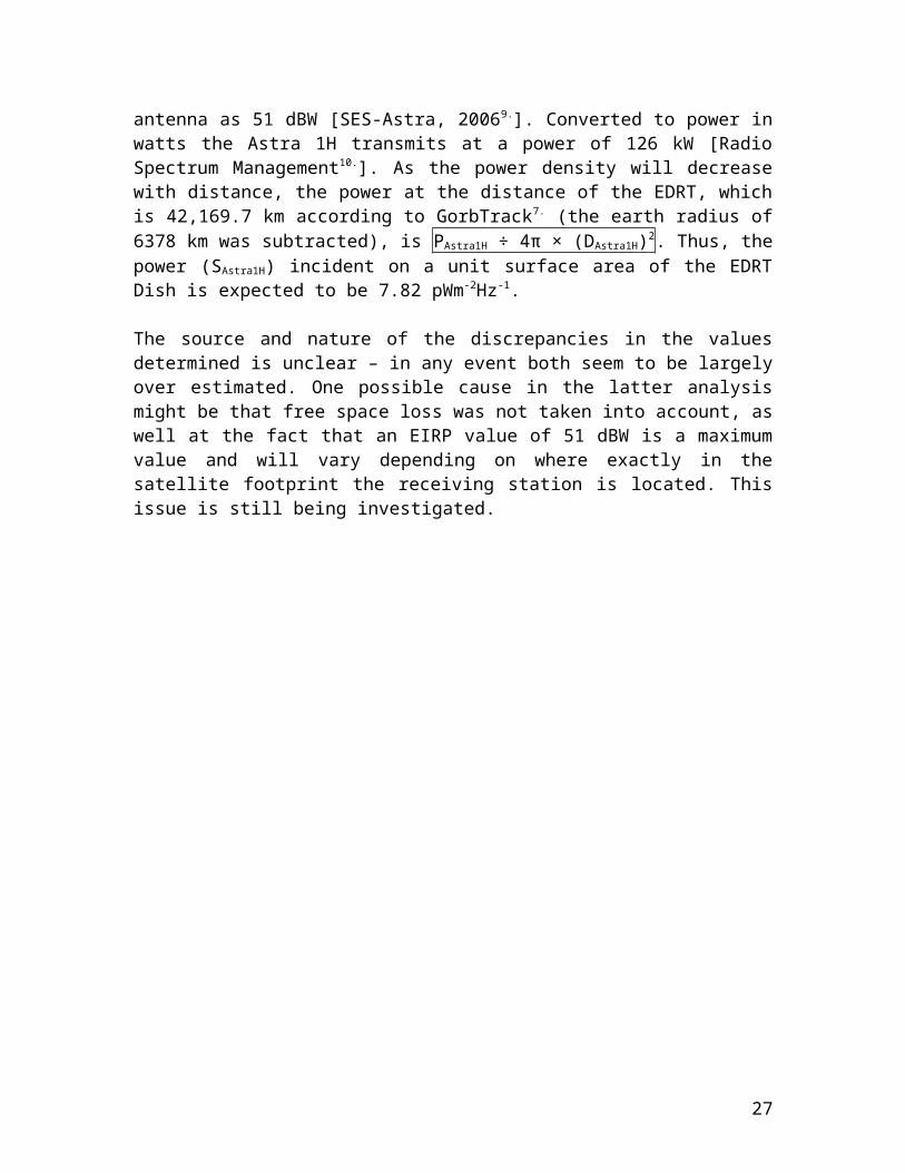
A modified plot of the solar drift scan of March 16, 2007 is presented below, where the coordinates are converted to degrees (Fig. 25). The conversion was facilitated with the Cartes du Ciel software program [Chevalley et al., 200616] by entering the Sun’s position at the beginning and end of the scan, then using the time and Az degree differences to determine how fast the Sun moves across the EDRT sky per degree.

Solar Flux

41.0

42.0

43.0

44.0

45.0

46.0

47.0

48.0

49.0

50.0

0.0 2.0 4.0 6.1 8.1 10.1 12.1 14.1 16.2 18.2

Equivalent Degrees

Pow

er (d

BuV)

Fig. 25. Solar drift scan of March 16, 2007 [time converted to degrees]

The drift scan was performed by pointing the telescope to the position of the Sun 30 minutes ahead of time, then allowing it to drift into the EDRT beam. This procedure highlighted issues with the positioning accuracy of the telescope, as the peak did not occur at the position expected. While the telescope was set for a peak at 13:30 (9.1°), the peak occurred at 13:26 (8.1°), 4 minutes off, which corresponds to an uncertainty of ±1° in position. With this can, the Half Power Beam Width (HPBW) of the dish can also be estimated – i.e. the width of the beam 3 dB below the peak. In this case the HPBW is estimated at 2.3°.

A Date with the Moon

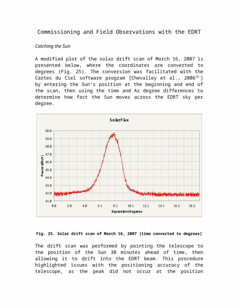
A lunar scan (Fig. 26) was achieved on March 03, 2007 at circa 00:00 UT by commanding the EDRT to move to the Moon’s position at that time, with the intention of producing a half lunar drift scan. However the plot below was instead observed, where, instead of a half bell curve, a full bell curve was produced.

Lunar Flux

44

44.1

44.2

44.3

44.4

44.5

44.6

1:01

:26

1:02

:03

1:02

:41

1:03

:20

1:03

:58

1:04

:36

1:05

:14

1:05

:52

1:06

:30

1:07

:07

1:07

:45

1:08

:23

1:09

:01

1:09

:39

1:10

:17

1:10

:54

1:11

:32

1:12

:10

1:12

:49

1:13

:27

1:14

:05

1:14

:43

1:15

:21

1:15

:59

1:16

:37

Time (HH:MM:SS)

Pow

er (d

BuV)

Fig. 26. Drift scan of the Moon (times shown are local time)

This illustrates that the Moon’s pass through the antenna beam was delayed by approximately 7 minutes, suggesting that the antenna was centered on the wrong position. In 7 minutes the Moon would have moved by 2° which illustrates the magnitude of the uncertainty, and reinforces the uncertainty range of 1° – 3° determined previously with the Astra 1H scans.

Charting the Radio Sky

As a final testimony to the capabilities of the EDRT, a motion to scan the entire Ku Band radio environment visible to the ISU EDRT was attempted1.

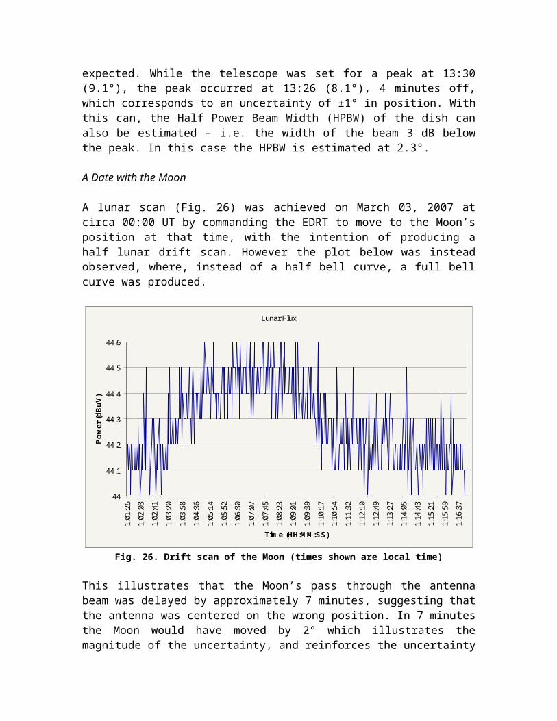
The first scan was completed on February 14, 2007, dubbed “The Valentine Scan” (Fig. 27). It was achieved in good time by scanning in Az from 90° – 270° with the Az speed switch set to “Slow”. The Az scans were done with 2° steps in elevation.

1 The colormap images were generated in Matlab by simply producing a matrix from the mass of data and using the 3D plotting functionality of Matlab (“surf” and “contour” in this case) to generate the plots. The colormap was produced by the “shading interp” Matlab function.

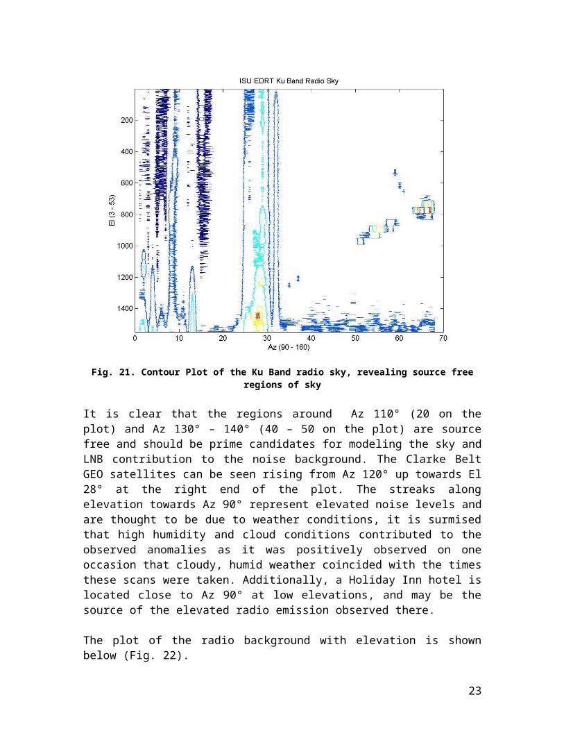
Fig. 27. The Valentine Scan of the ISU EDRT Ku Band radio environment

There is a discontinuity at the lowest elevation, as illustrated on the El axis, where an 4°step was made. This was due to the fact that an El of -6° means the telescope was pointing at the ground, which would have a constant flux between -6° and -2°.

The Astra 1H satellite stands out powerfully at Az 164° (as given in GorbTrack7). Another powerful radio source stands out above the lower elevation background at approximately Az 237°, El 16° (see Fig. 17), which can be identified with the PAS 3 satellite of Panamsat – it is co-located with the PAS 6B satellite but is the only of the pair with coverage over Europe.

To achieve higher resolution and sensitivity, another scanning method was employed, where the pulsed tracking mode of the RadioAstro software was used. The pulsed scanning allows higher dwell time in a single position, thus increasing sensitivity and allowing for the averaging of noise fluctuations. The caveat, as noted with the Astra 1H scans (Fig. 19, Fig. 20) is that unpredictable jumps of 2° or 3° are done. The scans were made in El from 53° to 7°, below which the software does not allow the telescope to point (also consider the offsets previously identified when calibrating the positioning accuracy). If lower elevations were required this would have to be done manually. Each scan consumed 50 minutes of time with some 1550 measurements per scan, and, to

achieve greater resolution, the scans were done in steps of Az 1°. As should be apparent, the task of covering the full 180° of sky that was covered in the Valentine Scan would take approximately 150 hrs to complete – more than the time officially allotted to the entirety of this project. The scans were done from Az 90° up to Az 180°, thus covering 90° Az and about 1/8 th of the EDRT radio sky. One result is shown below (Fig. 28).

Fig. 28. EDRT Ku Band radio environment covering Az 90° – 180° and El 7° – 53°

The increased sensitivity of the system is evident with satellites being revealed in the radio sky, which were not evident above the background in the Valentine Scan. Astra 1H is, however, still king of the Ku Band radio sky, standing some 10 dBµV above its neighbors in power.

The contour image, below (Fig. 29) facilitates better visual correlation between the distinct radio sources and the Clarke Belt plots in Fig. 17 and Fig. 18.

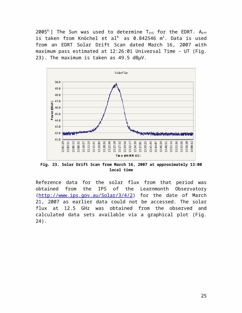
Fig. 29. Contour image of the ISU radio sky from Az 90° – 180° and El 7° – 53°

With reference to the aforementioned figures and GorbTrack7 a satellite candidate can be identified with each prominent radio source.

The satellite radio sources, start from approximately Az 118°, El 15° with Intelsat 902, Az 147°, El 27° – Intelsat 802, Az 157°, El 30° – Arabsat 3A, Astra 1H, and stop at a few possible candidates for Az 184°, El 34° – Astra 1C, HotBird 3 and Az 186°, El 33° – Telecom 2C.

Additionally, the noisy environment at Az 90° – 100° may be identified with the Holiday Inn hotel that is situated in that position relative to the EDRT location. As previously noted with Fig. 21, the vertical streaks are associated with increased background noise, which coincide with cloudy and humid weather.

In an attempt to expose more subtleties in the sky image, the contour plot was logarithmized, thus compressing the range between very high and very low power values, and making the lower values more visible. The logarithmic contour plot – below (Fig. 30) – greatly exposes the Clarke Belt as seen by the EDRT; more satellites are exposed in the area of the sky appearing empty in the above plots and their emissions are seen to overlap. Astra 1H powerfully emitting in the red regions of the contour, and indeed being the broadest satellite source, however, remains king of the ISU EDRT radio sky.

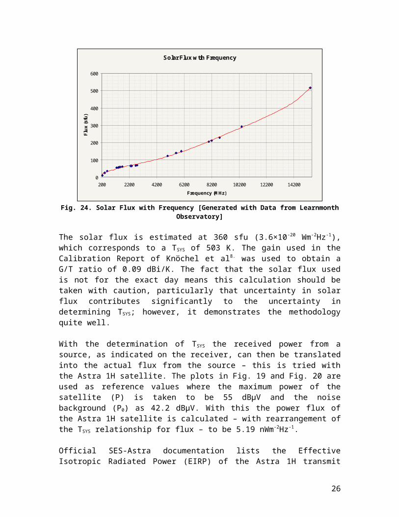
Fig. 30. The Clarke Belt Exposed (Astra 1H still stands out)

Lessons Learned from the ISU EDRT

This trial run with the ESA-Dresden Radio Telescope (EDRT) illustrated that it is a good teaching tool, which can stimulate interest in the numerous areas of science that are applicable to the project. It also has the potential to highlight many of the issues scientists have to face with larger, more sensitive, and more complex installations, be that attractive or detractive.

Undertaken in this report was a brief look at the history of radio science, starting from Tesla, Lodge, Braun, Popov and Marconi’s early attempts to communicate with radio waves. Society’s dependence on radio communications today was highlighted with a few examples of the applications of radio communications technologies. The rise of radio astronomy was also threaded into this history. The shortage of radio astronomy education below the specialized level in educational institutions was highlighted, where cost and size of the facilities required were seen as major inhibitors to implementation. Some low cost solutions in existence were mentioned.

It was seen that the EDRT functions reasonably within the domain identified in the reports and manuals that accompanied the equipment.

It was surmised that access to the location of the EDRT be taken actively into consideration at first installation. The windload on the ISU EDRT was estimated and illustrated that sustained winds of greater than 110 km/hr had the potential to topple IOU. Windspeeds of greater than 95 km per hour can topple the configuration illustrated in the manual which had less ballast than the IOU. Safety concerns were expressed regarding the Rubber Band and its potential to dislodge and backlash causing serious injury or damage. Lightening protection was also an issue and steps were taken to protect the ISU EDRT and its users.

Calibration highlighted the inaccuracies in the positioning of the ISU EDRT which, in the normal “Go to Position” mode of the RadioAstro software, is up to 2°. In the pulsed tracking mode of RadioAstro, the system positioning had a resolution of 1° – 3°. The positioning inaccuracies were also highlighted when attempts at drift scans of the Sun or Moon were made, where they were missed by up to 2°.

The system detected the Sun and Moon with power levels comparable to those reported in previous reports and manuals, which suggests that its sensitivity is up to specifications. The G/T ratio of the EDRT was tentatively calculated to be 0.09 dBi/K, which is at the lower end of the sensitivity spectrum for radio dishes.

A mapping of the radio sky that can be seen by the ISU EDRT was started and completed at a reasonably high resolution (in terms of integration time) from 90° to 180°. The Clarke Belt of geostationary satellites was exposed in the radio sky

mapping and satellites were identified, some with greater certainty than others. This was a rather time intensive endeavour.

Other projects that are currently underway include an analysis of scans were the telescope was left at one position in the sky to attempt a capture of radio emission from the galactic centre. There were some regular variations observed on first glance bases, and it was decided these were worth looking into. It is not yet certain whether or not the galactic centre was detected, but there were several consistent peaks at the time it was expected to rise.

In short, the analysis of the capabilities of ISU EDRT is still well underway as there are many more activities that can be carried out with the system. One may envision joint interferometric observations using EDRTs at different installations. This would introduce students to the cutting edge of current radio science techniques. It can be seen where students will enjoy the experience with the telescope, while gaining solid hands on experience and grasping fundamental skills and knowledge in the ways of science and engineering.

References2

1. PBS.org. Tesla Life and Legacy – Coming to America, Who Invented Radio?. [online].Url: http://www.pbs.org/tesla/ll/ll_whoradio.html [accessed 17/03/07].

2. Radio Astronomy Tutorial. The History of Radio Astronomy. [online].Url: http://www.haystack.edu/edu/undergrad/materials/tut4.html [accessed 17/03/07].

3. Salah, J.E., Pratap, P., Rogers, A.E.E. 2003. The Educational Role of Small Telescopes in Radio Astronomy. T.D. Oswalt (ed.), The Future of Small Telescopes in the New Millenium. Vol. II, 323-336. Kluwer Academic Publishers, Printed in the Netherlands.

4. Knöchel, U., Haiduk, F., Fritzsche, B.. 2005. Radio Astronomy at Schools. European Space Agency Contract Report. Contract 18369/04/NL/CP. Fraunhofer-Institut für Integrierte Schaltungen. November 02, 2005.

5. Assembly Manual of the ESA-Dresden Radio Telescope, European Space Agency Contract Report: Radio Astronomy at Schools. Contract 18369/04/NL/CP. Fraunhofer-Institut für Integrierte Schaltungen. September 2005

6. Google Earth 4.0.2722, Build Date, Jan 5 2007, Build Time: 11:17:17, Renderer: OpenGL, Operating System: Microsoft Windows XP (Service Pack 2), Video Driver: ATI Technologies Inc. (00006.00014.00010.06546), Max Texture Size: 2048x2048, Server: kh.google.com

7. Walda, B. 2004. GorbTrack version 0.4. January, 2004. Lelystad, The Netherlands. gorbtrack@hotmail.com.Url: http://members.chello.nl/~berry.walda/

8. Knöchel, U., Haiduk, F.. 2005. Calibration Report. European Space Agency Contract Report. Contract 18369/04/NL/CP. Fraunhofer-Institut für Integrierte Schaltungen. August 08, 2005.

9. SES-Astra. 2006. Astra 1H Factsheet. [online]. November 2006.Url: http://www.ses-astra.com/corpSite/documentsShared/satellite_factsheets/0_1H_Footprint_FactSheet.pdf [accessed 20/03/07].

2 Harvard Reference style adapted from: Anglia Ruskin University, University Library. 2007. Guide to Harvard Referencing System. [online]. February 19, 2007Url: http://libweb.anglia.ac.uk/referencing/harvard.htm#3.11. [accessed 17/03/07].

10.Ministry of Economic Development. Radio Spectrum Management. Information Library. dbW / Watts Converter. [online].Url: http://www.rsm.govt.nz/formsfees/dbw-watts.html. [accessed 21/03/07].

11.ANTWINDTM. Updated June 03, 1998. Distributed by Andrew Corporation. [online].Url: http://www.andrew.com/downloads/antwind/default.aspx. [accessed 21/03/07].

12.SES-Astra. 2006. Channel Finder – TV. [online].Url: http://www.ses-astra.com/backoffice/findAChannel_en/index.php?action=viewChannel&channelID=364. [accessed 21/07/2007].

13.Sullivvan, W.T. 2004. Discovery and First Observations of the 21-CM Hydrogen Line. Bulletin of the American Astronomical Society, 37 #3. [online].Url: http://www.aas.org/publications/baas/v37n3/dps2005/799.htm. [accessed 22/03/07].

14.Aerodyn. 2006. Data Base. Drag Coefficients for Bluff Bodies. Advanced Topics in Aerodynamics. Release 4.1.1. September 206. [online].Url: http://aerodyn.org/. [accessed 18/01/07].

15.Elert, G. Students. 2006. Density of Air. The Physics Factbook. [online].Url: http://hypertextbook.com/facts/2000/RachelChu.shtml. [accessed 18/01/07].

16.Chevalley, P., Dean, P. 2006. Carted de Ciel Version 3 beta 0.1.2. December 03, 2006, 19:03:55. [online].Url: http://www.ap-i.net/skychart. [accessed 13/01/2007].