Astro 321Set 1: FRW Cosmology

Wayne Hu

FRW Cosmology• The Friedmann-Robertson-Walker (FRW sometimes Lemaitre,

FLRW) cosmology has two elements

• The FRW geometry or metric

• The FRW dynamics or Einstein/Friedmann equation(s)

• Same as the two pieces of General Relativity (GR)

• A metric theory: geometry tells matter how to move

• Field equations: matter tells geometry how to curve

• Useful to separate out these two pieces both conceptually and forunderstanding alternate cosmologies, e.g.

• Modifying gravity while remaining a metric theory

• Breaking the homogeneity or isotropy assumption under GR

FRW Geometry• FRW geometry = homogeneous and isotropic on large scales

• Universe observed to be nearly isotropic (e.g. CMB, radio pointsources, galaxy surveys)

• Copernican principle: we’re not special, must be isotropic to allobservers (all locations)

Implies homogeneity

Verified through galaxy redshift surveys

• FRW cosmology (homogeneity, isotropy & field equations)generically implies the expansion of the universe, except forspecial unstable cases

Isotropy & Homogeneity• Isotropy: CMB isotropic to 10−3, 10−5 if dipole subtracted

• Redshift surveys show return to homogeneity on the >100Mpcscale

COBE DMR Microwave Sky at 53GHz

SDSS Galaxies

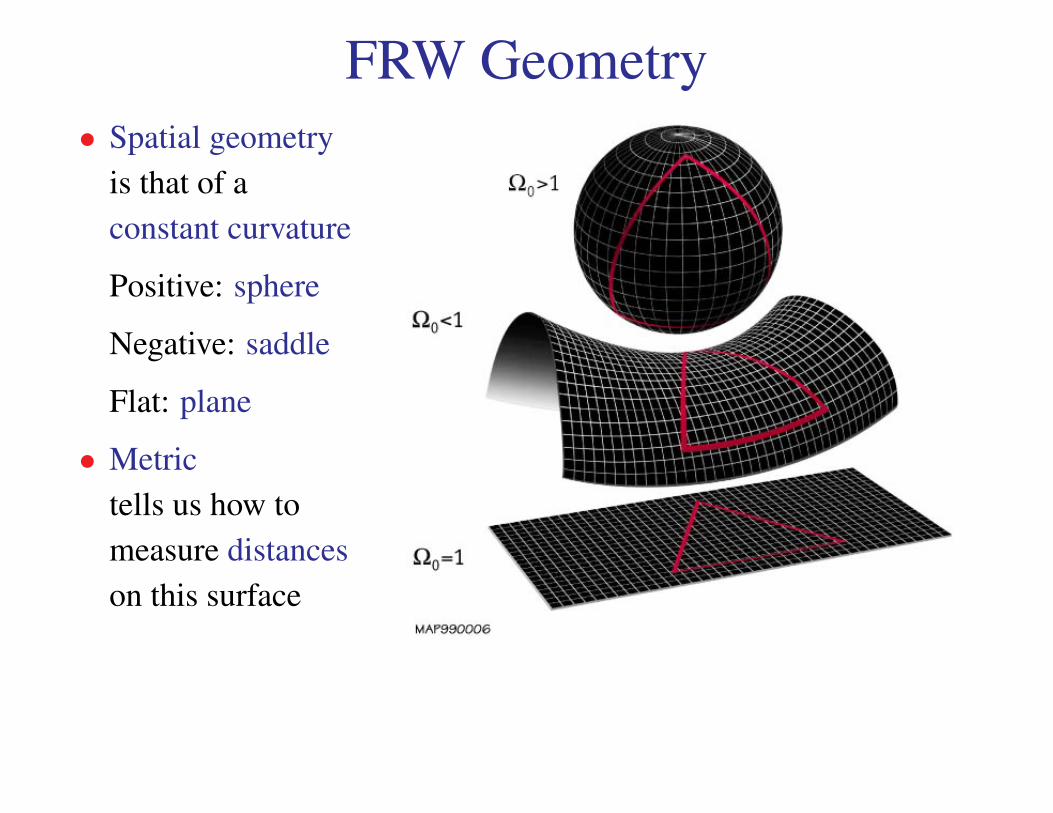
FRW Geometry. • Spatial geometry

is that of aconstant curvature

Positive: sphere

Negative: saddle

Flat: plane

• Metrictells us how tomeasure distanceson this surface

FRW Geometry• Closed geometry of a sphere of radius R

• Suppress 1 dimension α represents total angular separation (θ, φ)

dD

D

dα

DAdα

D A=

Rsin(D

/R)

dΣ

FRW Geometry• Two types of distances:• Radial distance on the arc D

Distance (for e.g. photon) traveling along the arc• Angular diameter distance DA

Distance inferred by the angular separation dα for a knowntransverse separation (on a constant latitude) DAdα

Relationship DA = R sin(D/R)

• As if background geometry (gravitationally) lenses image

• Positively curved geometry DA < D and objects are further thanthey appear

• Negatively curved universe R is imaginary andR sin(D/R) = i|R| sin(D/i|R|) = |R| sinh(D/|R|)

and DA > D objects are closer than they appear

Angular Diameter Distance• 3D distances restore usual spherical polar angles

dΣ2 = dD2 +D2Adα

2

= dD2 +D2A(dθ2 + sin2 θdφ2)

• GR allows arbitrary choice of coordinates, alternate notation is touse DA as radial coordinate

• DA useful for describing observables (flux, angular positions)

• D useful for theoretical constructs (causality, relationship totemporal evolution)

Angular Diameter Distance• The line element is often also written using DA as the coordinate

distance

dD2A =

(dDA

dD

)2

dD2

(dDA

dD

)2

= cos2(D/R) = 1− sin2(D/R) = 1− (DA/R)2

dD2 =1

1− (D2A/R)2

dD2A

and defining the curvature K = 1/R2 the line element becomes

dΣ2 =1

1−D2AK

dD2A +D2

A(dθ2 + sin2 θdφ2)

where K < 0 for a negatively curved space

Volume Element• Metric also defines the volume element

dV = (dD)(DAdθ)(DA sin θdφ)

= D2AdDdΩ

where dΩ = sin θdθdφ is solid angle

• Most of classical cosmology boils down to these three quantities,(comoving) radial distance, (comoving) angular diameter distance,and volume element

• For example, distance to a high redshift supernova, angular size ofthe horizon at last scattering and BAO feature, number density ofclusters...

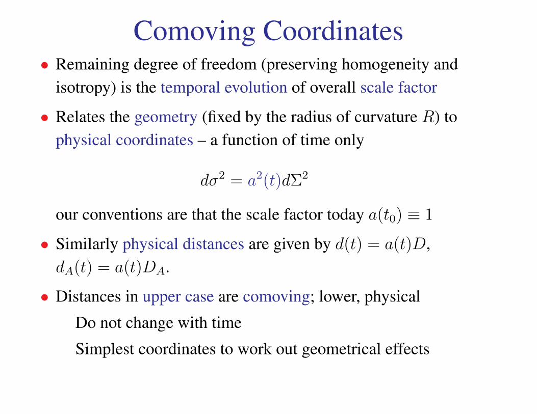
Comoving Coordinates• Remaining degree of freedom (preserving homogeneity and

isotropy) is the temporal evolution of overall scale factor

• Relates the geometry (fixed by the radius of curvature R) tophysical coordinates – a function of time only

dσ2 = a2(t)dΣ2

our conventions are that the scale factor today a(t0) ≡ 1

• Similarly physical distances are given by d(t) = a(t)D,dA(t) = a(t)DA.

• Distances in upper case are comoving; lower, physical

Do not change with time

Simplest coordinates to work out geometrical effects

Time and Conformal Time• Proper time (with c = 1)

dτ 2 = dt2 − dσ2

= dt2 − a2(t)dΣ2

• Taking out the scale factor in the time coordinate

dτ 2 ≡ a2(t) (dη2 − dΣ2)

dη = dt/a defines conformal time – useful in that photonstravelling radially from observer then obey

∆D = ∆η =

∫dt

a

so that time and distance may be interchanged

Horizon• Distance travelled by a photon in the whole lifetime of the universe

defines the horizon

• Since dτ = 0, the horizon is simply the elapsed conformal time

Dhorizon(t) =

∫ t

0

dt′

a= η(t)

• Horizon always grows with time

• Always a point in time before which two observers separated by adistance D could not have been in causal contact

• Horizon problem: why is the universe homogeneous and isotropicon large scales especially for objects seen at early times, e.g.CMB, when horizon small

FRW Metric• Proper time defines the metric gµν

dτ 2 ≡ gµνdxµdxν

Einstein summation - repeated lower-upper pairs summed

Signature follows proper time convention (rather than properlength, compatibility with Peacock’s book - I tend to favorlength so beware I may mess up overall sign in lectures)

• Usually we will use comoving coordinates and conformal time asthe xµ unless otherwise specified – metric for other choices arerelated by a(t)

• We will avoid real General Relativity but rudimentary knowledgeuseful

Hubble Parameter• Useful to define the expansion rate or Hubble parameter

H(t) ≡ 1

a

da

dt=d ln a

dt

fractional change in the scale factor per unit time - ln a = N is alsoknown as the e-folds of the expansion

• Cosmic time becomes

t =

∫dt =

∫d ln a

H(a)

• Conformal time becomes

η =

∫dt

a=

∫d ln a

aH(a)

Redshift.

Recession Velocity

Expansion Redshift

• Wavelength of light “stretches”with the scale factor

• Given an observed wavelengthtoday λ, physical restwavelength at emission λ0

λ =1

a(t)λ0 ≡ (1 + z)λ0

δλ

λ0

=λ− λ0

λ0

= z

• Interpreting the redshift as a Doppler shift, objects recede in anexpanding universe

Distance-Redshift Relation• Given atomically known rest wavelength λ0, redshift can be

precisely measured from spectra

• Combined with a measure of distance, distance-redshiftD(z) ≡ D(z(a)) can be inferred

• Related to the expansion history as

D(a) =

∫dD =

∫ 1

a

d ln a′

a′H(a′)

[d ln a′ = −d ln(1 + z) = −a′dz]

D(z) = −∫ 0

z

dz′

H(z′)=

∫ z

0

dz′

H(z′)

Hubble Law• Note limiting case is the Hubble law

limz→0

D(z) = z/H(z = 0) ≡ z/H0

independently of the geometry and expansion dynamics

• Hubble constant usually quoted as as dimensionless h

H0 = 100h km s−1Mpc−1

• Observationally h ∼ 0.7 (see below)

• With c = 1, H−10 = 9.7778 (h−1 Gyr) defines the time scale

(Hubble time, ∼ age of the universe)

• As well as H−10 = 2997.9 (h−1 Mpc) a length scale (Hubble scale

∼ Horizon scale)

Measuring D(z)• Standard Ruler: object of known physical size

λ = a(t)Λ

subtending an observed angle α on the sky α

α =Λ

DA(z)≡ λ

dA(z)

dA(z) = aDA(a) =DA(z)

1 + z

where, by analogy to DA, dA is the physical angular diameterdistance

• Since DA → Dhorizon whereas (1 + z) unbounded, angular size ofa fixed physical scale at high redshift actually increases with radialdistance

Measuring D(z)• Standard Candle: object of known luminosity L with a measured

flux S (energy/time/area)

• Comoving surface area 4πD2A

• Frequency/energy redshifts as (1 + z)

• Time-dilation or arrival rate of photons (crests) delayed as(1 + z):

F =L

4πD2A

1

(1 + z)2≡ L

4πd2L

• So luminosity distance

dL = (1 + z)DA = (1 + z)2dA

• As z → 0, dL = dA = DA

Olber’s Paradox• Surface brightness

S =F

∆Ω=

L

4πd2L

d2A

λ2

• In a non-expanding geometry (regardless of curvature), surfacebrightness is conserved dA = dL

S = const.

• So since each site line in universe full of stars will eventually endon surface of star, night sky should be as bright as sun (not infinite)

• In an expanding universe

S ∝ (1 + z)−4

Olber’s Paradox• Second piece: age finite so even if stars exist in the early universe,

not all site lines end on stars

• But even as age goes to infinity and the number of site lines goesto 100%, surface brightness of distant objects (of fixed physicalsize) goes to zero

• Angular size increases

• Redshift of energy and arrival time

Measuring D(z)• Ratio of fluxes or difference in log flux (magnitude) measurable

independent of knowing luminosity

m1 −m2 = −2.5 log10(F1/F2)

related to dL by definition by inverse square law

m1 −m2 = 5 log10[dL(z1)/dL(z2)]

• If absolute magnitude is known

m−M = 5 log10[dL(z)/10pc]

absolute distances measured, e.g. at low z = z0 Hubble constant

dL ≈ z0/H0 → H0 = z0/dL

• Also standard ruler whose length, calibrated in physical units

Measuring D(z)• If absolute calibration of standards unknown, then both standard

candles and standard rulers measure relative sizes and fluxes

For standard candle, e.g. compare magnitudes low z0 to a high zobject involves

∆m = mz −mz0 = 5 log10

dL(z)

dL(z0)= 5 log10

H0dL(z)

z0

Likewise for a standard ruler comparison at the two redshifts

dA(z)

dA(z0)=

H0dA(z)

z0

• Distances are measured in units of h−1 Mpc.

• Change in expansion rate measured as H(z)/H0

Hubble Constant. • Hubble in 1929 used the

Cepheid period luminosityrelation to infer distances tonearby galaxies therebydiscovering the expansionof the universe

• Hubble actually inferred too large a Hubble constant ofH0 ∼ 500km/s/Mpc

• Miscalibration of the Cepheid distance scale - absolutemeasurement hard, checkered history

• H0 now measured as 74.2± 3.6km/s/Mpc by SHOES calibratingoff AGN water maser

Hubble Constant History• Took 70 years to settle on this value with a factor of 2 discrepancy

persisting until late 1990’s

• Difficult measurement since local galaxies where individualCepheids can be measured have peculiar motions and so theirvelocity is not entirely due to the “Hubble flow”

• A “distance ladder” of cross calibrated measurements

• Primary distanceindicators cepheids, novae planetary nebula orglobular cluster luminosity function, AGN water maser

• Use more luminous secondary distance indications to go out indistance to Hubble flow

Tully-Fisher, fundamental plane, surface brightnessfluctuations, Type 1A supernova

Maser-Cepheid-SN Distance Ladder.

1500 13001400

1

2

3

4

0

Flux

Den

sity

(Jy)

550 450 -350 -450

0.1 pc

2.9 mas

10 5 0 -5 -10Impact Parameter (mas)

-1000

0

1000

2000

LOS

Vel

ocity

(km

/s)

Herrnstein et al (1999)NGC4258

• Water maser aroundAGN, gas in Keplerian orbit

• Measure proper motion,radial velocity, accelerationof orbit

• Method 1: radial velocity plusorbit infer tangential velocity = distance × angular proper motion

vt = dA(dα/dt)

• Method 2: centripetal acceleration and radial velocity from lineinfer physical size

a = v2/R, R = dAθ

Maser-Cepheid-SN Distance Ladder• Calibrate Cepheid period-luminosity relation in same galaxy

• SHOES project then calibrates SN distance in galaxies withCepheids

Also: consistent with recent HST parallax determinations of 10galactic Cepheids (8% distance each) with ∼ 20% larger H0

error bars - normal metalicity as opposed to LMC Cepheids.

• Measure SN at even larger distances out into the Hubble flow

• Riess et al H0 = 74.2± 3.6km/s/Mpc more precise (5%) than theHST Key Project calibration (11%).

• Ongoing VLBI surveys are trying to find Keplerian water masersystems directly out in the Hubble flow (100 Mpc) to eliminaterungs in the distance ladder

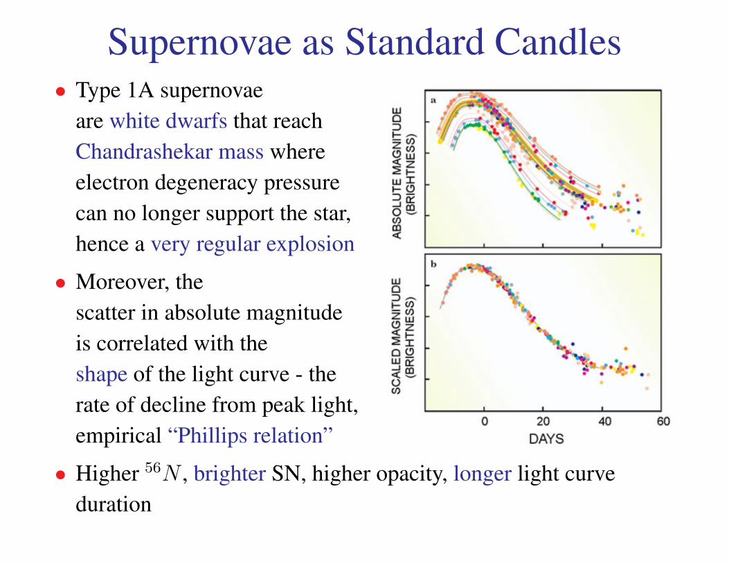
Supernovae as Standard Candles. • Type 1A supernovae

are white dwarfs that reachChandrashekar mass whereelectron degeneracy pressurecan no longer support the star,hence a very regular explosion

• Moreover, thescatter in absolute magnitudeis correlated with theshape of the light curve - therate of decline from peak light,empirical “Phillips relation”

• Higher 56N , brighter SN, higher opacity, longer light curveduration

Beyond Hubble’s Law.

14

16

18

20

22

24

0.0 0.2 0.4 0.6 0.8 1.01.0

0.5

0.0

0.5

1.0

mag

. res

idua

lfr

om e

mpt

y co

smol

ogy

0.25,0.750.25, 0 1, 0

0.25,0.75

0.25, 0

1, 0

redshift z

Supernova Cosmology ProjectKnop et al. (2003)

Calan/Tololo& CfA

SupernovaCosmologyProject

effe

ctiv

e m

B

ΩΜ , ΩΛ

ΩΜ , ΩΛ

• Type 1A are therefore“standardizable” candlesleading to a very lowscatter δm ∼ 0.15 and visibleout to high redshift z ∼ 1

• Two groups in 1999found that SN more distant ata given redshift than expected

• Cosmic acceleration

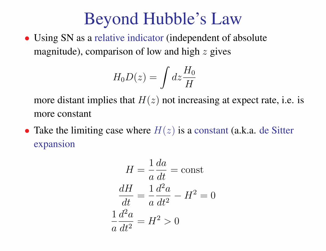
Beyond Hubble’s Law• Using SN as a relative indicator (independent of absolute

magnitude), comparison of low and high z gives

H0D(z) =

∫dzH0

H

more distant implies that H(z) not increasing at expect rate, i.e. ismore constant

• Take the limiting case where H(z) is a constant (a.k.a. de Sitterexpansion

H =1

a

da

dt= const

dH

dt=

1

a

d2a

dt2−H2 = 0

1

a

d2a

dt2= H2 > 0

Beyond Hubble’s Law• Indicates that the expansion of the universe is accelerating

• Intuition tells us (FRW dynamics shows) ordinary matterdecelerates expansion since gravity is attractive

• Ordinary expectation is that

H(z > 0) > H0

so that the Hubble parameter is higher at high redshift

• Or equivalently that expansion rate decreases as it expands

FRW Dynamics• This is as far as we can go on FRW geometry alone - we still need

to know how the scale factor a(t) evolves given matter-energycontent

• General relativity: matter tells geometry how to curve, scale factordetermined by content

• Build the Einstein tensor Gµν out of the metric and use Einsteinequation (overdots conformal time derivative)

Gµν( = Rµν −1

2gµνR) = −8πGTµν

G00 = − 3

a2

[(a

a

)2

+1

R2

]

Gij = − 1

a2

[2a

a−(a

a

)2

+1

R2

]δij

Einstein Equations• Isotropy demands that the stress-energy tensor take the form

T 00 = ρ

T ij = −pδij

where ρ is the energy density and p is the pressure

• It is not necessary to assume that the content is a perfect fluid -consequence of FRW symmetry

• So Einstein equations become(a

a

)2

+1

R2=

8πG

3a2ρ

2a

a−(a

a

)2

+1

R2= −8πGa2p

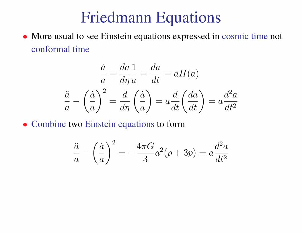
Friedmann Equations• More usual to see Einstein equations expressed in cosmic time not

conformal time

a

a=da

dη

1

a=da

dt= aH(a)

a

a−(a

a

)2

=d

dη

(a

a

)= a

d

dt

(da

dt

)= a

d2a

dt2

• Combine two Einstein equations to form

a

a−(a

a

)2

= −4πG

3a2(ρ+ 3p) = a

d2a

dt2

Friedmann Equations• Friedmann equations:

H2(a) +1

a2R2=

8πG

3ρ

1

a

d2a

dt2= −4πG

3(ρ+ 3p)

• Acceleration source is ρ+ 3p requiring p < −3ρ for positiveacceleration

• Curvature as an effective energy density component

ρK = − 3

8πGa2R2∝ a−2

Critical Density• Friedmann equation for H then reads

H2(a) =8πG

3(ρ+ ρK) ≡ 8πG

3ρc

defining a critical density today ρc in terms of the expansion rate

• In particular, its value today is given by the Hubble constant as

ρc(z = 0) =3H2

0

8πG= 1.8788× 10−29h2g cm−3

• Energy density today is given as a fraction of critical

Ω ≡ ρ

ρc(z = 0)

• Note that physical energy density ∝ Ωh2 (g cm−3)

Critical Density• Likewise radius of curvature then given by

ΩK = (1− Ω) = − 1

H20R

2→ R = (H0

√Ω− 1)−1

• If Ω ≈ 1, then true density is near critical ρ ≈ ρc and

ρK ρc ↔ H0R 1

Universe is flat across the Hubble distance

• Ω > 1 positively curved

DA = R sin(D/R) =1

H0

√Ω− 1

sin(H0D√

Ω− 1)

• Ω < 1 negatively curved

DA = R sin(D/R) =1

H0

√1− Ω

sinh(H0D√

1− Ω)

Newtonian Energy Interpretation• Consider a test particle of mass m as part of expanding spherical

shell of radius r and total mass M .

.

r

mv

M=4πr3ρ/3

• Energy conservation

E =1

2mv2 − GMm

r= const

1

2

(dr

dt

)2

− GM

r= const

1

2

(1

r

dr

dt

)2

− GM

r3=

const

r2

H2 =8πGρ

3− const

a2

Newtonian Energy Interpretation. • Constant determines whether

the system is bound andin the Friedmann equation isassociated with curvature – notgeneral since neglects pressure

• Nonetheless Friedmannequation is the same withpressure - but mass-energywithin expanding shell is not constant

• Instead, rely on the fact that gravity in the weak field regime isNewtonian and forces unlike energies are unambiguously definedlocally.

Newtonian Force Interpretation• An alternate, more general Newtonian derivation, comes about by

realizing that locally around an observer, gravity must lookNewtonian.

• Given Newton’s iron sphere theorem, the gravitational accelerationdue to a spherically symmetric distribution of mass outside someradius r is zero (Birkhoff theorem in GR)

• We can determine the acceleration simply from the enclosed mass

∇2ΨN = 4πG(ρ+ 3p)

∇ΨN =4πG

3(ρ+ 3p)r =

GMN

r2

where ρ+ 3p reflects the active gravitational mass provided bypressure.

Newtonian Force Interpretation• Hence the gravitational acceleration

r

r= −1

r∇ΨN = −4πG

3(ρ+ 3p)

• We’ll come back to this way of viewing the effect of the expansionon spherical collapse including the dark energy.

Conservation Law• The two Friedmann equation are redundant in that one can be

derived from the other via energy conservation

• (Consequence of Bianchi identities in GR:∇µGµν = 0)

dρV + pdV = 0

dρa3 + pda3 = 0

ρa3 + 3a

aρa3 + 3

a

apa3 = 0

ρ

ρ= −3(1 + w)

a

a

• Time evolution depends on “equation of state” w(a) = p/ρ

• If w = const. then the energy density depends on the scale factoras ρ ∝ a−3(1+w).

Multicomponent Universe• Special cases:

• nonrelativistic matter ρm = mnm ∝ a−3, wm = 0

• ultrarelativistic radiation ρr = Enr ∝ νnr ∝ a−4, wr = 1/3

• curvature ρK ∝ a−2, wK = −1/3

• (cosmological) constant energy density ρΛ ∝ a0, wΛ = −1

• total energy density summed over above

ρ(a) =∑i

ρi(a) = ρc(a = 1)∑i

Ωia−3(1+wi)

• If constituent w also evolve (e.g. massive neutrinos)

ρ(a) = ρc(a = 1)∑i

Ωie−

∫d ln a 3(1+wi)

Multicomponent Universe• Friedmann equation gives Hubble parameter evolution in a

H2(a) = H20

∑Ωie

−∫d ln a 3(1+wi)

• In fact we can always define a critical equation of state

wc =pcρc

=

∑wiρi − ρK/3∑i ρi + ρK

• Critical energy density obeys energy conservation

ρc(a) = ρc(a = 1)e−∫d ln a 3(1+wc(a))

• And the Hubble parameter evolves as

H2(a) = H20e−

∫d ln a 3(1+wc(a))

Acceleration Equation• Time derivative of (first) Friedmann equation

dH2

dt=

8πG

3

dρcdt

2H

[1

a

d2a

dt2−H2

]=

8πG

3H[−3(1 + wc)ρc][

1

a

d2a

dt2− 2

4πG

3ρc

]= −4πG

3[3(1 + wc)ρc]

1

a

d2a

dt2= −4πG

3[(1 + 3wc)ρc]

= −4πG

3(ρ+ ρK + 3p+ 3pK)

= −4πG

3(1 + 3w)ρ

• Acceleration equation says that universe decelerates if w > −1/3

Expansion Required• Friedmann equations “predict” the expansion of the universe.

Non-expanding conditions da/dt = 0 and d2a/dt2 = 0 require

ρ = −ρK ρ = −3p

i.e. a positive curvature and a total equation of statew ≡ p/ρ = −1/3

• Since matter is known to exist, one can in principle achieve this byadding a balancing cosmological constant

ρ = ρm + ρΛ = −ρK = −3p = 3ρΛ

ρΛ = −1

3ρK , ρm = −2

3ρK

Einstein introduced ρΛ for exactly this reason – “biggest blunder”;but note that this balance is unstable: ρm can be perturbed but ρΛ, atrue constant cannot

Cosmic Microwave Radiation• Existence of a ∼ 10K radiation background predicted by Gamow

and Alpher in 1948 based on the formation of light elements in ahot big bang (BBN)

• Peebles, Dicke, Wilkinson & Roll in 1965 independently predictedthis background and proceeded to build instrument to detect it

• Penzias & Wilson 1965 found unexplained excess isotropic noisein a communications antennae and learning of the Peebles et alcalculation announced the discovery of the blackbody radiation

• Thermal radiation proves that the universe began in a hot densestate when matter and radiation was in equilibrium - ruling out acompeting steady state theory

Cosmic Microwave Radiation• Modern measurement from COBE satellite of blackbody

spectrum. T = 2.725K giving Ωγh2 = 2.471× 10−5

frequency (cm–1)

Bν

(× 1

0–5 )

GHz

error × 50

50

2

4

6

8

10

12

10 15 20

200 400 600

Cosmic Microwave Radiation• Radiation is isotropic to 10−5 in temperature→ horizon problem

Total Radiation• Adding in neutrinos to the radiation gives the total radiation (next

lecture set) content as Ωrh2 = 4.153× 10−5

• Since radiation redshifts faster than matter by one factor of 1 + z

even this small radiation content will dominate the total energydensity at sufficiently high redshift

• Matter-radiation equality

1 + zeq =Ωmh

2

Ωrh2

1 + zeq = 3130Ωmh

2

0.13

Dark Matter• Since Zwicky in the 1930’s non-luminous or dark matter has been

known to dominate over luminous matter in stars (and hot gas)

• Arguments based on internal motion holding system up againstgravitational force

• Equilibrium requires a balance pressure of internal motions

rotation velocity of spiral galaxies

velocity dispersion of galaxies in clusters

gas pressure or thermal motion in clusters

radiation pressure in CMB acoustic oscillations

Classical Argument• Classical argument for measuring total amount of dark matter

• Assuming that the object is somehow typical in its non-luminousto luminous density: “mass-to-light ratio”

• Convert to dark matter density as M/L× luminosity density

• From galaxy surveys the luminosity density in solar units is

ρL = 2± 0.7× 108hLMpc−3

(h’s: L ∝ Fd2 so ρL ∝ L/d3 ∝ d−1 and d in h−1 Mpc

• Critical density in solar units is

ρc = 2.7754× 1011h2MMpc−3

so that the critical mass-to-light ratio in solar units is

M/L ≈ 1400h

Dark Matter: Rotation Curves. • Flat rotation curves:

GM/r2 ≈ v2/r

M ≈ v2r/G

so M ∝ r out to tens of kpc

• Implies M/L > 30h

and perhaps more –closure if flat out to ∼ 1 Mpc.

• Mass required to keep rotationcurves flat much larger than implied by stars and gas.

• Hence “dark” matter

Dark Matter: Clusters• Similar argument holds in clusters of galaxies

• Velocity dispersion replaces circular velocity

• Centripetal force is replaced by a “pressure gradient” T/m = σ2

and p = ρT/m = ρσ2

• Zwicky got M/L ≈ 300h.

• Generalization to the gas distribution also gives evidence for darkmatter

Dark Matter: Bullet Cluster• Merging clusters: gas (visible matter) collides and shocks (X-rays),

dark matter measured by gravitational lensing passes through

Hydrostatic Equilibrium• Evidence for dark matter in X-ray clusters also comes from direct

hydrostatic equilibrium inference from the gas: balance radialpressure gradient with gravitational potential gradient

• Infinitesimal volume of area dA and thickness dr at radius r andinterior mass M(r): pressure difference supports the gas

[pg(r)− pg(r + dr)]dA =GmM

r2=GρgM

r2dV

dpgdr

= −ρgdΦ

dr

with pg = ρgTg/m becomes

GM

r= −Tg

m

(d ln ρgd ln r

+d lnTgd ln r

)• ρg from X-ray luminosity; Tg sometimes taken as isothermal

CMB Hydrostatic Equilibrium• Same argument in the CMB with radiation pressure in the gas

balancing the gravitational potential gradients of linear fluctuations

• Best measurement of the dark matter density to date:Ωch

2 = 0.1109± 0.0056, Ωbh2 = (2.258± 0.057)× 10−2.

• Unlike other techniques, measures the physical density of the darkmatter rather than contribution to critical since the CMBtemperature sets the physical density and pressure of the photons

Gravitational Lensing• Mass can be directly measured in the gravitational lensing of

sources behind the cluster

• Strong lensing (giant arcs) probes central region of clusters

• Weak lensing (1-10%) elliptical distortion to galaxy image probesouter regions of cluster and total mass

Giant Arcs• Giant arcs in galaxy clusters: galaxies, source; cluster, lens

Cosmic Shear• On even larger scales, the large-scale structure weakly shears

background images: weak lensing

Dark Energy• Distance redshift relation depends on energy density components

H0D(z) =

∫dz

H0

H(a)

• SN dimmer, distance further than in a matter dominated epoch

• Hence H(a) must be smaller than expected in a matter onlywc = 0 universe where it increases as (1 + z)3/2

H0D(z) =

∫dze

∫d ln a 3

2(1+wc(a))

• Distant supernova Ia as standard candles imply that wc < −1/3 sothat the expansion is accelerating

• Consistent with a cosmological constant that is ΩΛ = 0.74

• Coincidence problem: different components of matter scaledifferently with a. Why are two components comparable today?

Cosmic Census• With h = 0.71 and CMB Ωmh

2 = 0.133, Ωm = 0.26 - consistentwith other, less precise, dark matter measures

• CMB provides a test of DA 6= D through the standard rulers of theacoustic peaks and shows that the universe is close to flat Ω ≈ 1

• Consistency has lead to the standard model for the cosmologicalmatter budget:

• 74% dark energy

• 26% non-relativistic matter (with 83% of that in dark matter)

• 0% spatial curvature