
ASTRAL Tutorial - Tandy Warnowtandy.cs.illinois.edu/astral-warnow-tutorial-v2.pdfASTRAL versions •...
51
ASTRAL Tutorial • Instructor: Tandy Warnow, [email protected] • Main developer: Siavash Mirarab, [email protected] • Github site: https://github.com/smirarab/ASTRAL • Email: [email protected] 1
Transcript of ASTRAL Tutorial - Tandy Warnowtandy.cs.illinois.edu/astral-warnow-tutorial-v2.pdfASTRAL versions •...
ASTRAL Tutorial
• Instructor: Tandy Warnow, [email protected]
• Main developer: Siavash Mirarab, [email protected]
• Github site: https://github.com/smirarab/ASTRAL
• Email: [email protected]
1
This tutorial• Basic ASTRAL approach and statistical consistency
• How to use ASTRAL
• Using Best ML gene trees instead of Multi-Locus Bootstrapping
• Collapsing low support branches
• Modifying the search space
• Whether to filter or not
• Using multiple individuals
• Using SIESTA with ASTRAL (handling multiple optimal solutions)
• Interpreting the output
• Understanding branch support
• Understanding branch lengths
• Literature about ASTRAL
• Another Symposium (right before Evolution 2018) on Phylogenomics, in Montpellier!
2
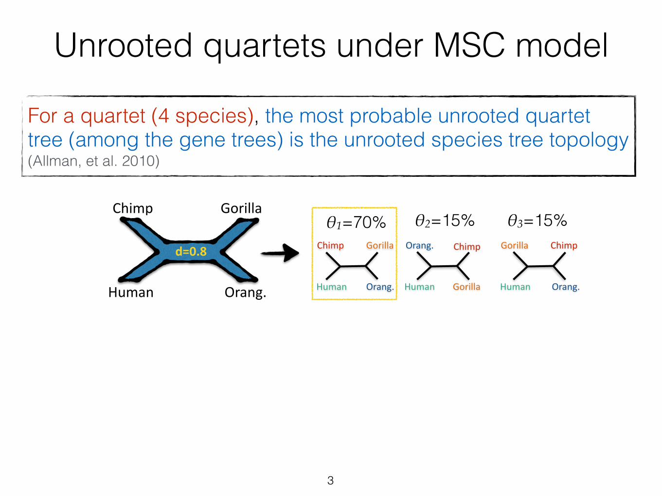
Unrooted quartets under MSC model
For a quartet (4 species), the most probable unrooted quartet tree (among the gene trees) is the unrooted species tree topology (Allman, et al. 2010)
3
Orang.
Gorilla Chimp
HumanOrang.
GorillaChimp
Human
Orang.
Gorilla
Chimp
Human
θ2=15% θ3=15%θ1=70%Gorilla
Orang.
Chimp
Human
d=0.8
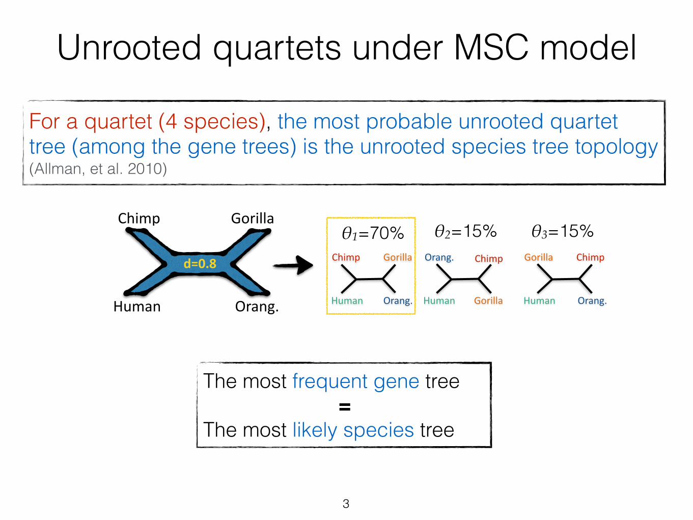
The most frequent gene tree = The most likely species tree
4
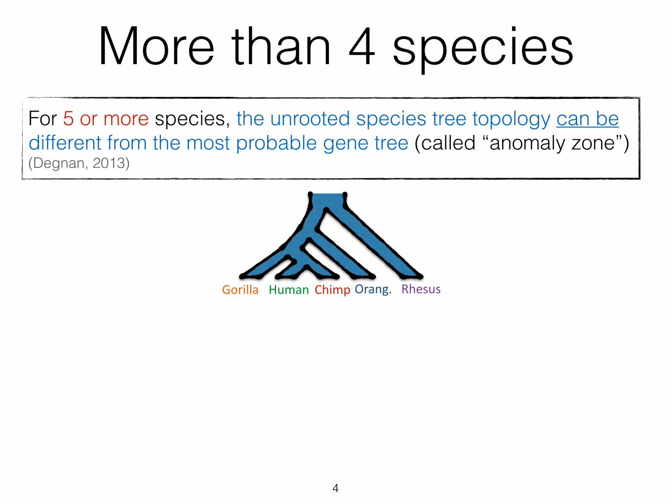
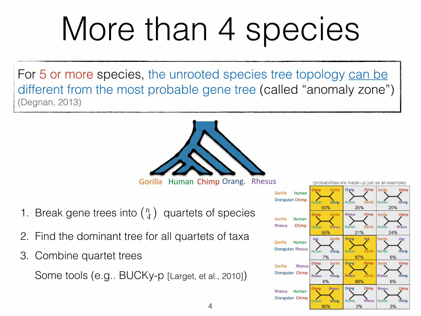
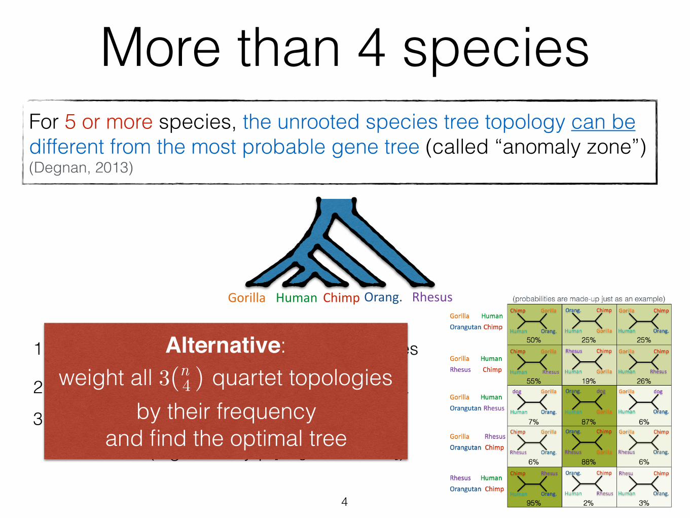
Orang.Gorilla ChimpHuman Rhesus
More than 4 speciesFor 5 or more species, the unrooted species tree topology can be different from the most probable gene tree (called “anomaly zone”) (Degnan, 2013)
4
Orang.Gorilla ChimpHuman Rhesus
1. Break gene trees into (n 4 ) quartets of species
2. Find the dominant tree for all quartets of taxa
3. Combine quartet trees
Some tools (e.g.. BUCKy-p [Larget, et al., 2010])
More than 4 speciesFor 5 or more species, the unrooted species tree topology can be different from the most probable gene tree (called “anomaly zone”) (Degnan, 2013)
Alternative: weight all 3(n
4 ) quartet topologies by their frequency
and find the optimal tree
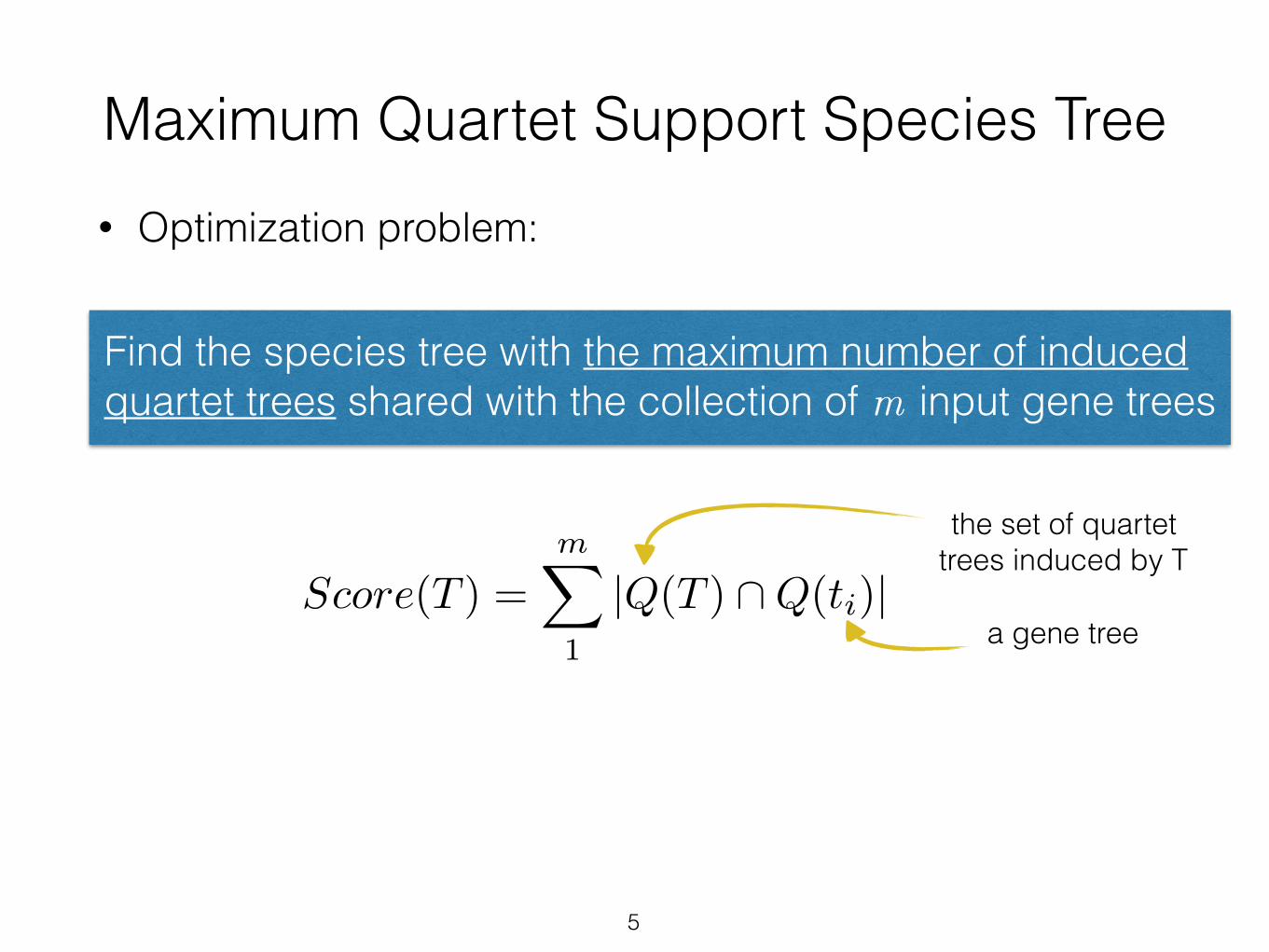
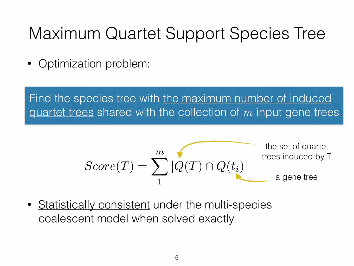
Maximum Quartet Support Species Tree• Optimization problem:
•
5
Find the species tree with the maximum number of induced quartet trees shared with the collection of m input gene trees
the set of quartet trees induced by T
a gene treeScore(T ) =
mX
1
|Q(T ) \Q(ti)|
Maximum Quartet Support Species Tree• Optimization problem:
•
• Statistically consistent under the multi-species coalescent model when solved exactly
5
Find the species tree with the maximum number of induced quartet trees shared with the collection of m input gene trees
the set of quartet trees induced by T
a gene treeScore(T ) =
mX
1
|Q(T ) \Q(ti)|
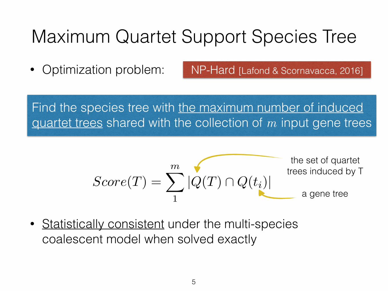
Maximum Quartet Support Species Tree• Optimization problem:
•
• Statistically consistent under the multi-species coalescent model when solved exactly
5
Find the species tree with the maximum number of induced quartet trees shared with the collection of m input gene trees
the set of quartet trees induced by T
a gene tree
NP-Hard [Lafond & Scornavacca, 2016]
Score(T ) =mX
1
|Q(T ) \Q(ti)|
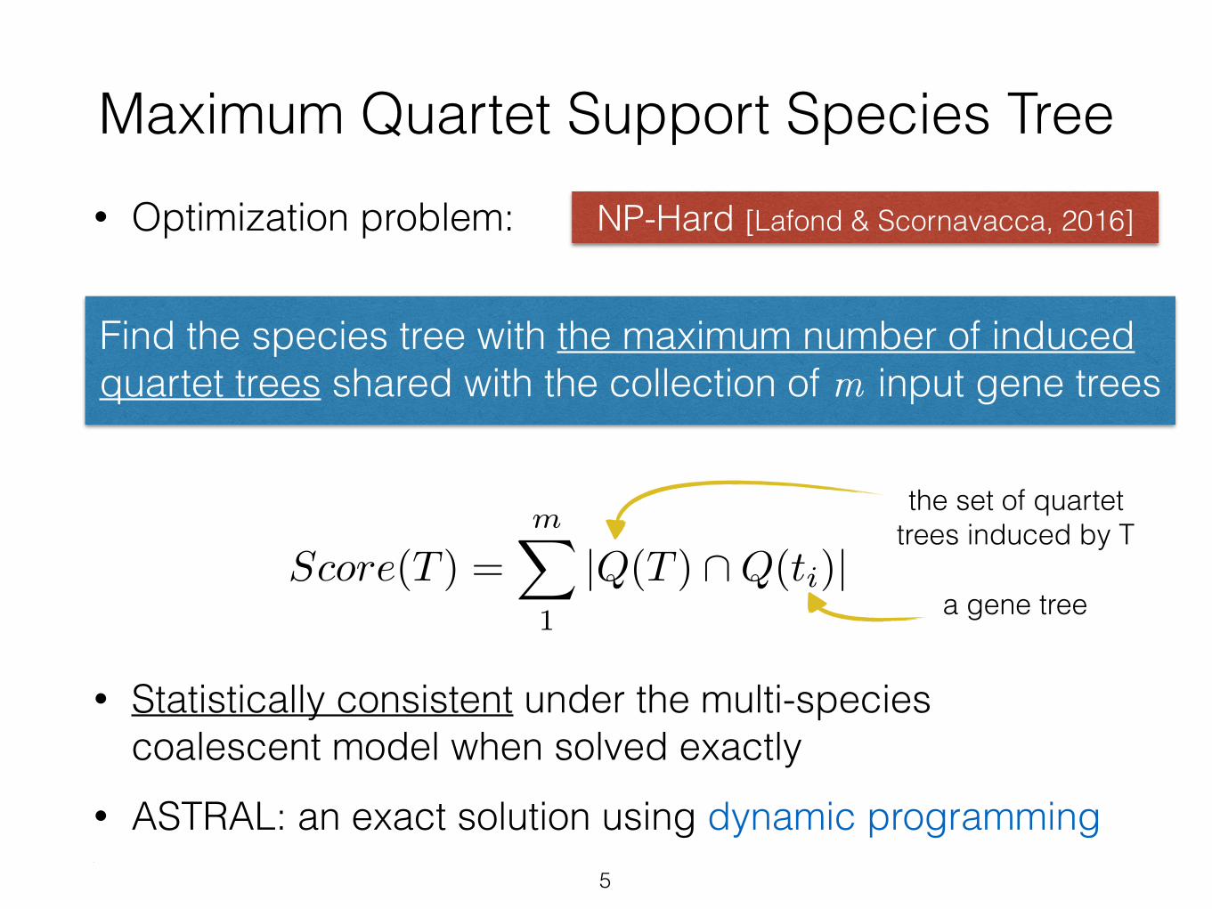
Maximum Quartet Support Species Tree• Optimization problem:
•
• Statistically consistent under the multi-species coalescent model when solved exactly
• ASTRAL: an exact solution using dynamic programming••
5
Find the species tree with the maximum number of induced quartet trees shared with the collection of m input gene trees
the set of quartet trees induced by T
a gene tree
NP-Hard [Lafond & Scornavacca, 2016]
Score(T ) =mX
1
|Q(T ) \Q(ti)|
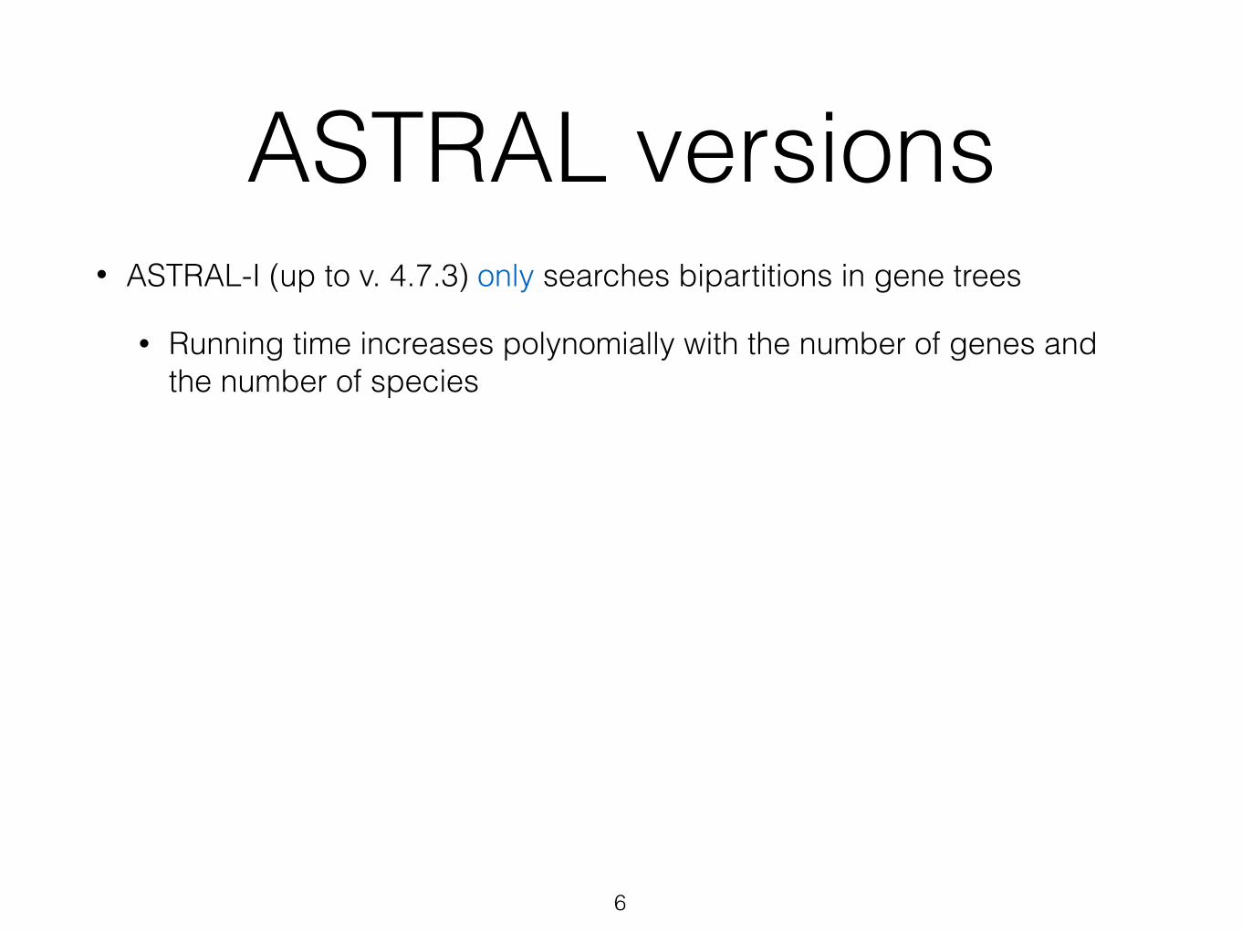
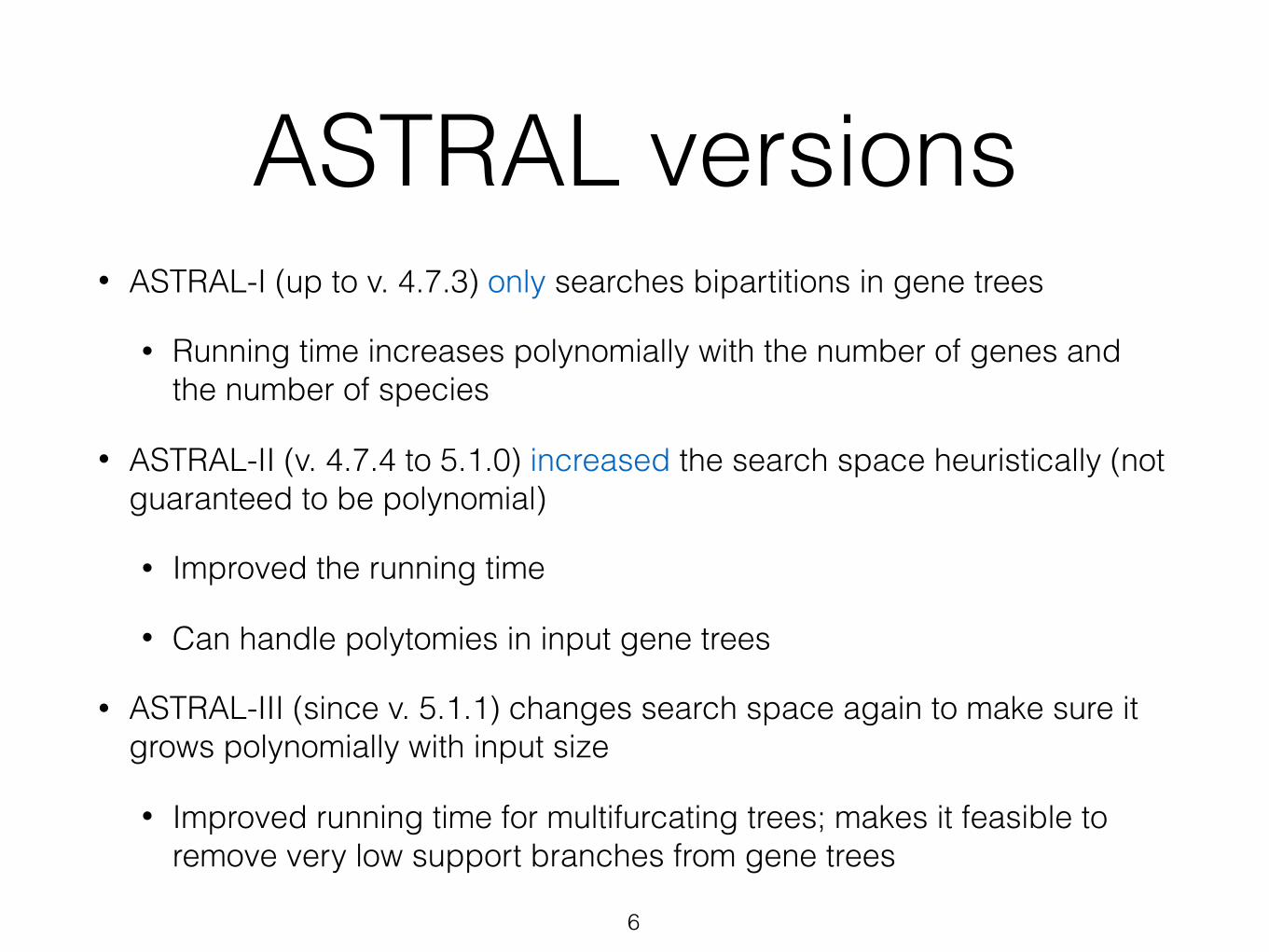
ASTRAL versions• ASTRAL-I (up to v. 4.7.3) only searches bipartitions in gene trees
• Running time increases polynomially with the number of genes and the number of species
6
ASTRAL versions• ASTRAL-I (up to v. 4.7.3) only searches bipartitions in gene trees
• Running time increases polynomially with the number of genes and the number of species
• ASTRAL-II (v. 4.7.4 to 5.1.0) increased the search space heuristically (not guaranteed to be polynomial)
• Improved the running time
• Can handle polytomies in input gene trees
• ASTRAL-III (since v. 5.1.1) changes search space again to make sure it grows polynomially with input size
• Improved running time for multifurcating trees; makes it feasible to remove very low support branches from gene trees
6
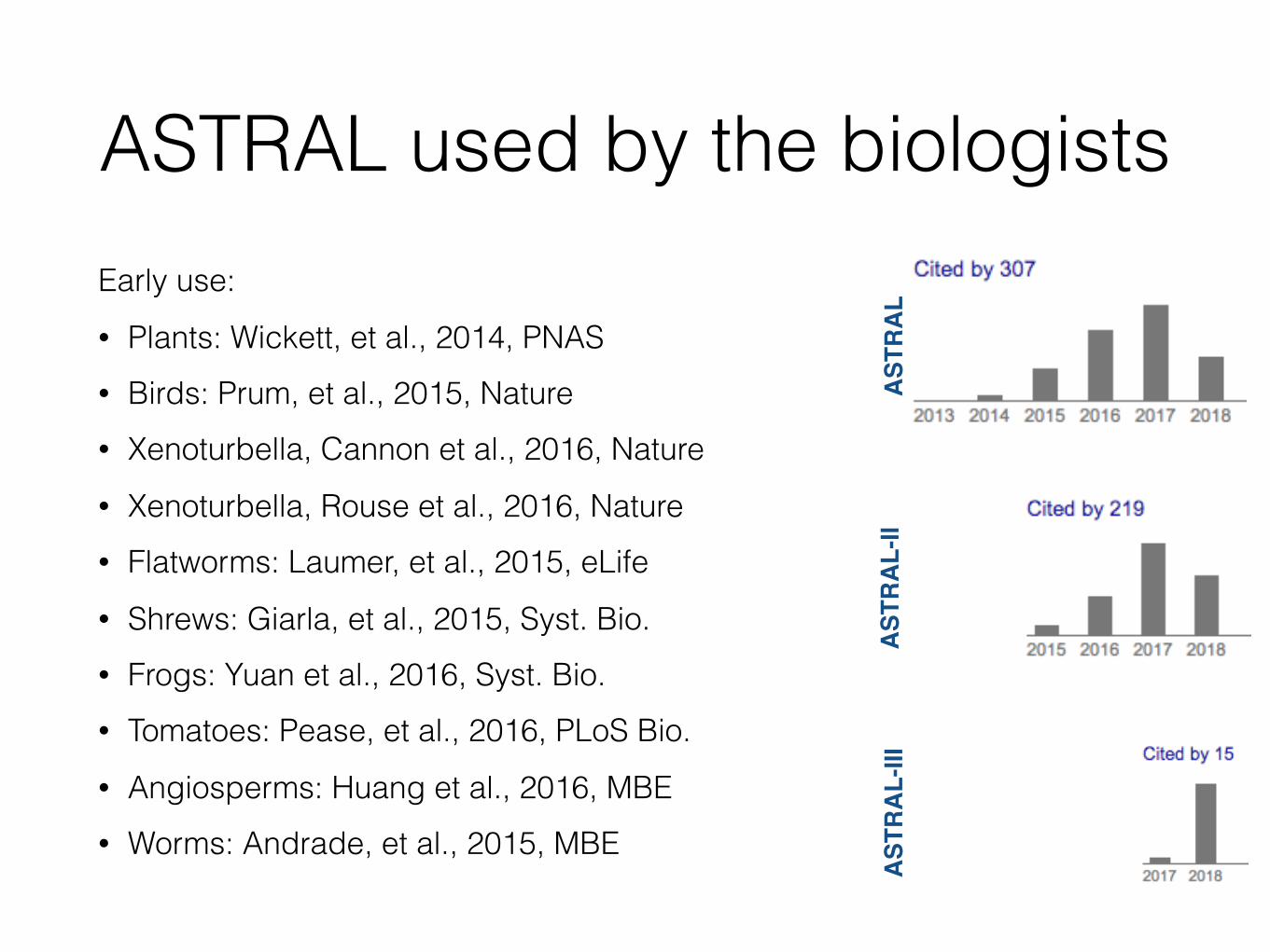
ASTRAL used by the biologistsEarly use: • Plants: Wickett, et al., 2014, PNAS • Birds: Prum, et al., 2015, Nature • Xenoturbella, Cannon et al., 2016, Nature • Xenoturbella, Rouse et al., 2016, Nature • Flatworms: Laumer, et al., 2015, eLife • Shrews: Giarla, et al., 2015, Syst. Bio. • Frogs: Yuan et al., 2016, Syst. Bio. • Tomatoes: Pease, et al., 2016, PLoS Bio. • Angiosperms: Huang et al., 2016, MBE • Worms: Andrade, et al., 2015, MBE
ASTRAL-II
ASTRAL
ASTRAL-III
bestML versus MLBS
8
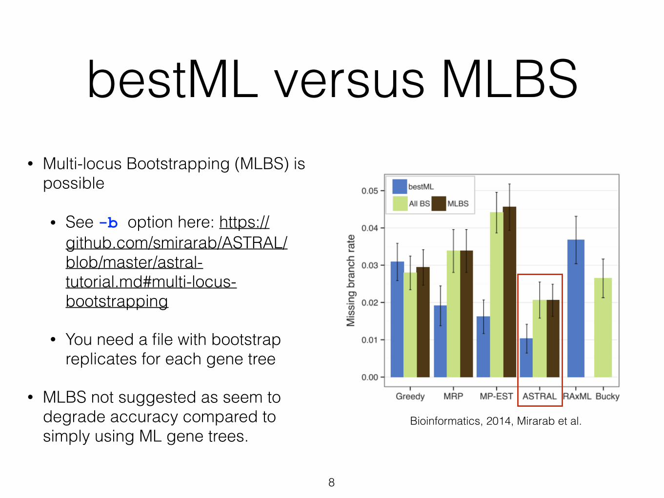
• Multi-locus Bootstrapping (MLBS) is possible
• See -b option here: https://github.com/smirarab/ASTRAL/blob/master/astral-tutorial.md#multi-locus-bootstrapping
• You need a file with bootstrap replicates for each gene tree
• MLBS not suggested as seem to degrade accuracy compared to simply using ML gene trees.
Bioinformatics, 2014, Mirarab et al.
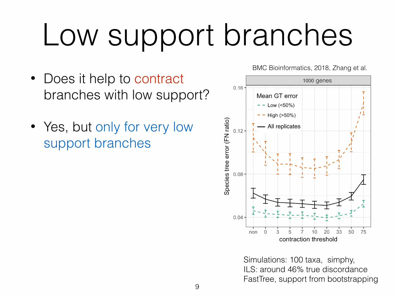
Low support branches• Does it help to contract
branches with low support?
• Yes, but only for very low support branches
9
Simulations: 100 taxa, simphy, ILS: around 46% true discordance FastTree, support from bootstrapping
genes
All replicates
BMC Bioinformatics, 2018, Zhang et al.
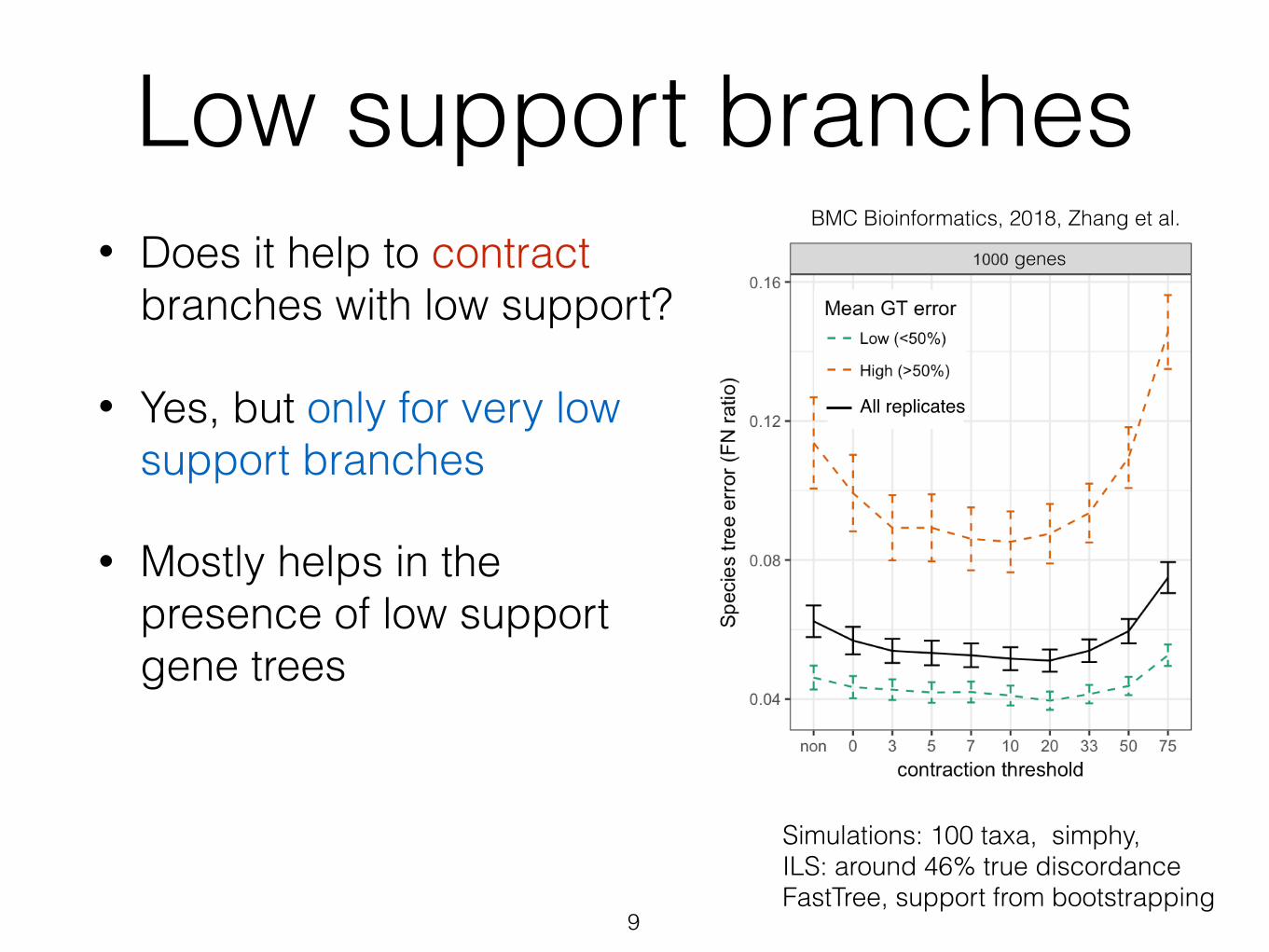
Low support branches• Does it help to contract
branches with low support?
• Yes, but only for very low support branches
• Mostly helps in the presence of low support gene trees
9
Simulations: 100 taxa, simphy, ILS: around 46% true discordance FastTree, support from bootstrapping
genes
All replicates
BMC Bioinformatics, 2018, Zhang et al.
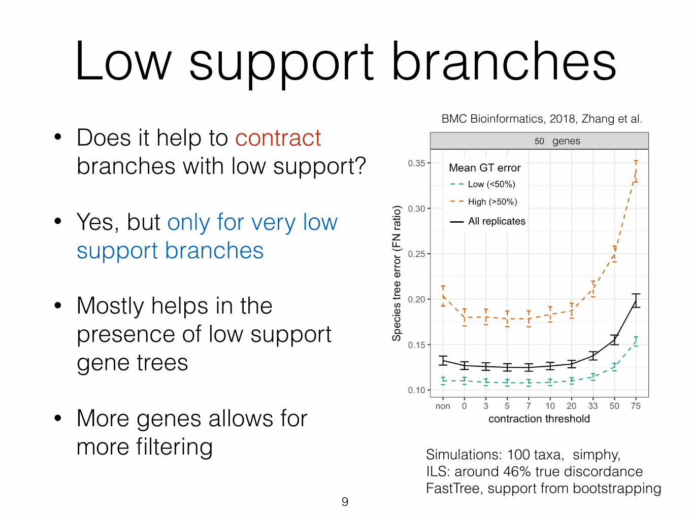
Low support branches• Does it help to contract
branches with low support?
• Yes, but only for very low support branches
• Mostly helps in the presence of low support gene trees
• More genes allows for more filtering
9
Simulations: 100 taxa, simphy, ILS: around 46% true discordance FastTree, support from bootstrapping
genes
All replicates
BMC Bioinformatics, 2018, Zhang et al.
Modifying the Search Space
• For small enough datasets, you can run ASTRAL in *exact* mode, which will find the globally optimal tree! (-x option)
• ASTRAL’s default usage will not run in exact mode, and will constrain the search space largely using the gene trees.
• It may be beneficial to *expand* the search space, using the “-e” or “-f” options (see tutorial at GitHub site). In particular, you can add species trees you’ve estimated using other methods, such as concatenation, SVDquartets, or species trees that other studies have suggested.
10
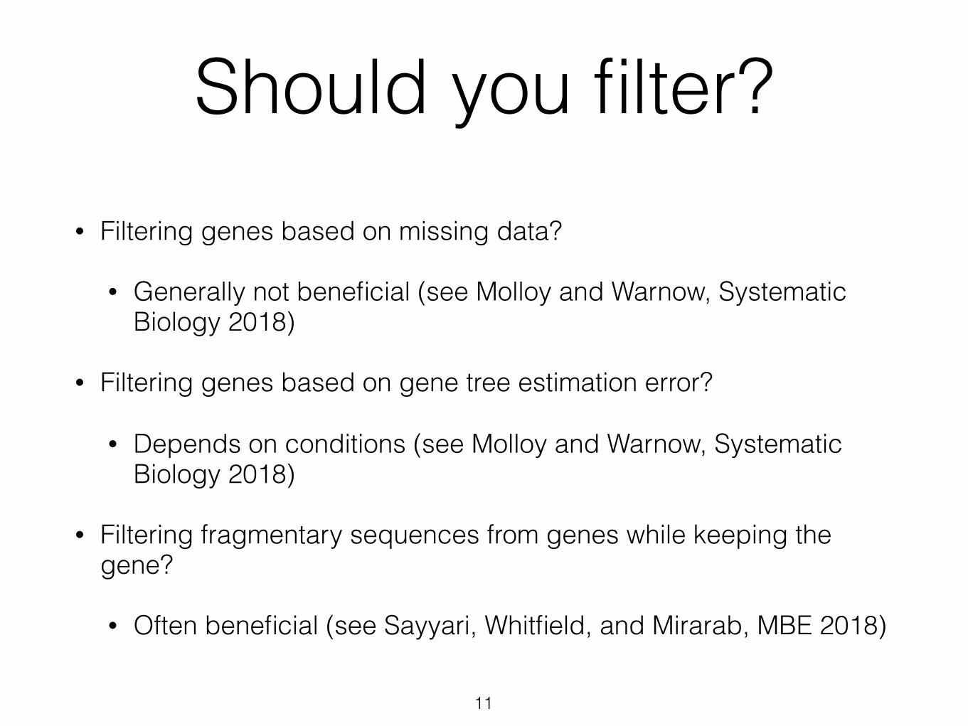
Should you filter?• Filtering genes based on missing data?
• Generally not beneficial (see Molloy and Warnow, Systematic Biology 2018)
• Filtering genes based on gene tree estimation error?
• Depends on conditions (see Molloy and Warnow, Systematic Biology 2018)
• Filtering fragmentary sequences from genes while keeping the gene?
• Often beneficial (see Sayyari, Whitfield, and Mirarab, MBE 2018)
11
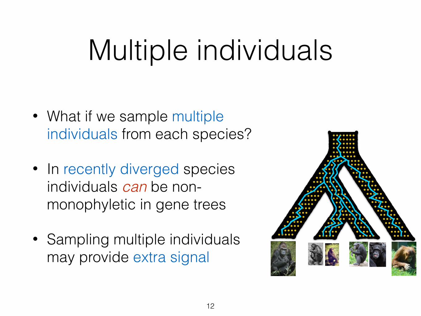
Multiple individuals
• What if we sample multiple individuals from each species?
• In recently diverged species individuals can be non-monophyletic in gene trees
• Sampling multiple individuals may provide extra signal
12
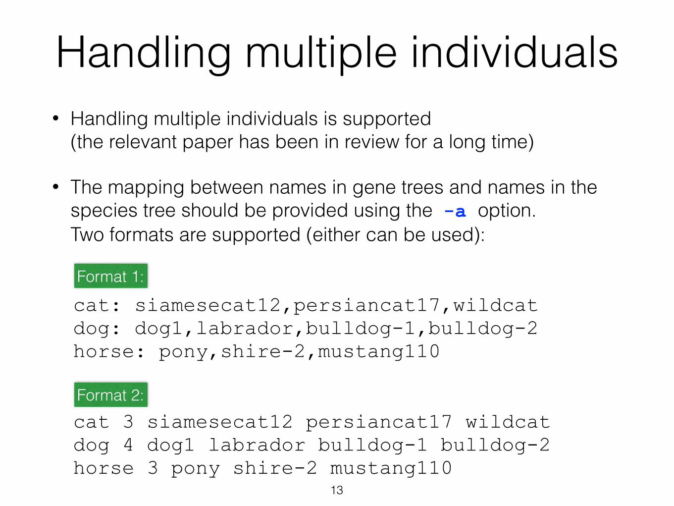
Handling multiple individuals• Handling multiple individuals is supported
(the relevant paper has been in review for a long time)
• The mapping between names in gene trees and names in the species tree should be provided using the -a option. Two formats are supported (either can be used):
13
cat: siamesecat12,persiancat17,wildcat dog: dog1,labrador,bulldog-1,bulldog-2 horse: pony,shire-2,mustang110
cat 3 siamesecat12 persiancat17 wildcat dog 4 dog1 labrador bulldog-1 bulldog-2 horse 3 pony shire-2 mustang110
Format 1:
Format 2:
Using SIESTA with ASTRAL
• ASTRAL solves an optimization problem, and there can be several optimal solutions.
• You can use SIESTA (Vachaspati and Warnow, BMC Genomics 2018) to enumerate the optimal trees and compute a consensus tree. Open source software at https://github.com/pranjalv123.
14

Interpreting the Output
15
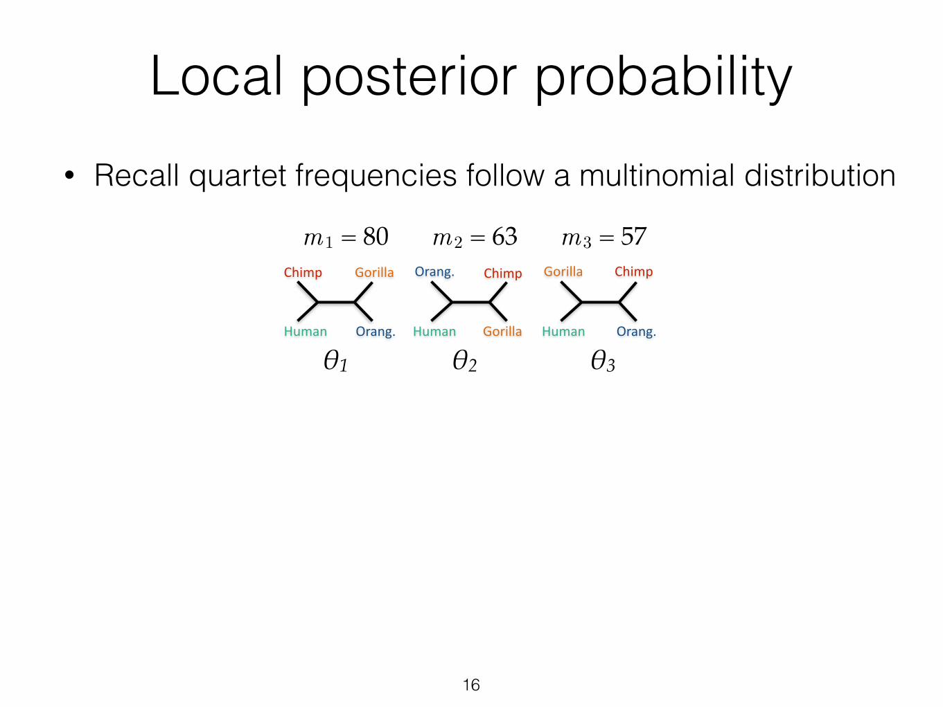
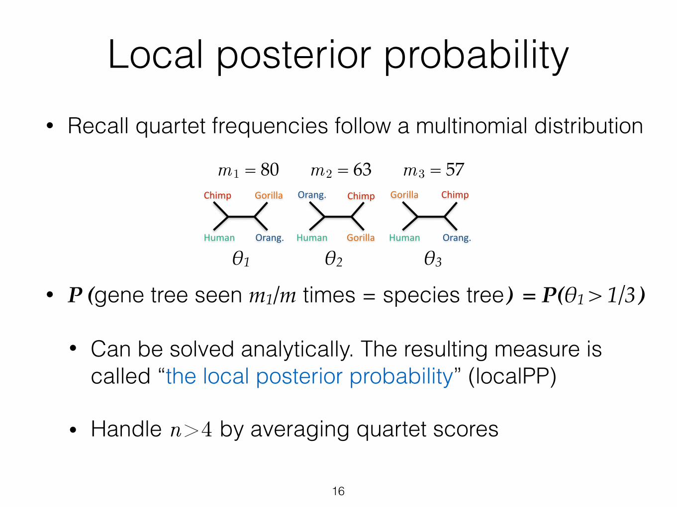
Local posterior probability• Recall quartet frequencies follow a multinomial distribution
16
Orang.
Gorilla Chimp
HumanOrang.
GorillaChimp
Human
Orang.
Gorilla
Chimp
Human
m2 = 63 m3 = 57m1 = 80
θ2 θ3θ1
Local posterior probability• Recall quartet frequencies follow a multinomial distribution
• P (gene tree seen m1/m times = species tree) = P(θ1 > 1/3)
• Can be solved analytically. The resulting measure is called “the local posterior probability” (localPP)
• Handle n>4 by averaging quartet scores
16
Orang.
Gorilla Chimp
HumanOrang.
GorillaChimp
Human
Orang.
Gorilla
Chimp
Human
m2 = 63 m3 = 57m1 = 80
θ2 θ3θ1
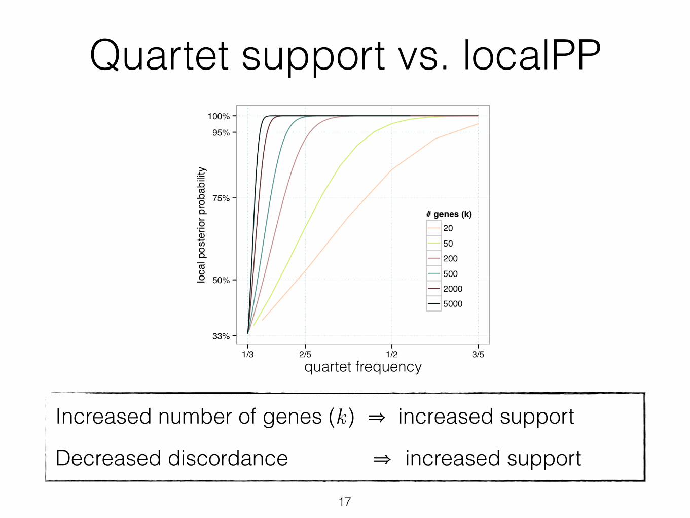
Quartet support vs. localPP
17
!3Background: How many targets are enough? The number of loci required for confidently resolving a phylogenetic relationship depends on its “hardness”. Discordant gene trees due to incomplete lineage sorting (ILS) can make branches of a species tree very difficult to resolve. ILS is a function of the branch length and population size. This means that shorter branches or larger population sizes increase ILS, and can make species tree reconstruction more difficult. The co-PI has recently developed a new approach for estimating the support of a branch in a coalescent-based framework based on the proportion of gene trees that support quartet topologies in gene trees[31]. This new approach is analogous to finding the probability that a three-sided die is loaded towards each facet by observing outcomes of many tosses. We can also ask the reverse question: if we have an estimate of the degree of bias of a die, how many tosses are needed to confidently find its loaded side. Similarly, this approach[31] sheds light on the relationship between the number of genes required to achieve a level of support for a branch of a certain length in coalescent units (Fig. 3). While the co-PI’s method of calculating support, which is implemented in ASTRAL [32, 33], gives the basic mathematical framework, more method development is needed (see below).
Research Approach Specimens Suitable specimens of more than 80 species of Sabellidae and >120 Terebelliformia species have been collected from localities around the world in the last 15 years by the PI. Further collecting will be undertaken for some key taxa for a few more transcriptomes and for targeted DNA capture. We also have agreements from other experts in Sabellidae and Terebelliformia to provide other needed ethanol-preserved specimens for targeted capture. We will obtain ~ 50% of the known sabellid diversity and ~25% of terebelliforms for targeted capture sequencing (~500 species total). Our plan is to sample all genera, particularly focusing on their type species. This should allow for the generation of robust phylogenies, from which we will revise the taxonomy. Specimens will be vouchered at the SIO Benthic Invertebrate Collection and biodiversity information curated on the Encyclopedia of Life. Sequencing (transcriptomes and targeted capture of DNA) A targeted capture approach will be used with an appropriate number of loci (see below) to generate robust phylogenies of Sabellidae and Terebelliformia. Two different sets of targets will be designed from transcriptomes, across Sabellidae and Terebelliformia repectively. We have already generated new transcriptomes for nine sabellids, a serpulid and a fabriciid (bold terminals in Fig. 4), and nine Terebelliformia (bold terminals in Fig. 5) and combined this data with the few publicly available transcriptomes. Based on direct sequencing data already obtained for several genes for Sabellidae and Terebelliformia [Rouse in prep.; Stiller et al. in prep.], our sampling arguably spans the extant diversity of each clade. Several more transcriptomes will be needed to ensure the targeted capture methods will be robust. Methods for generating these transcriptomes will follow those previously used by us[6, 34]. How many targets are needed? A targeted capture pipeline typically starts from a large number of loci sequenced from a small number of species using genome-wide approaches (e.g., transcriptomics)[7, 8, 35]. This initial dataset is then used to select a smaller subset of loci for the targeted capture phase, which involves a larger set of species. To reduce the cost and effort, one would want to minimize the number of loci in the second phase, as long as sufficient loci are selected to confidently resolve relationships of interest. To date the number of loci has been determined in an ad hoc manner, either by the ultra conserved elements discovered[7, 8] or limitations of the targeted capture technology[13]. Initial analyses of our two datasets demonstrates how the number of
Fig. 3. Impact of number of genes (colors) and amount of ILS (x-axis) on support (posterior probability) for a branch (y-axis). Under the coalescent model, for four species separated with an unrooted branch of length d, the probability of a gene tree being identical to the species tree is 1-2/3e-d (we use this as a measure of ILS). We measure support using local pp [31] for various numbers of gene trees (assuming no gene tree estimation error). More ILS (ie., low 1-2/3e-d) requires more genes to get high support.
quartet frequency
Increased number of genes (k ) ⇒ increased support
Decreased discordance ⇒ increased support
18
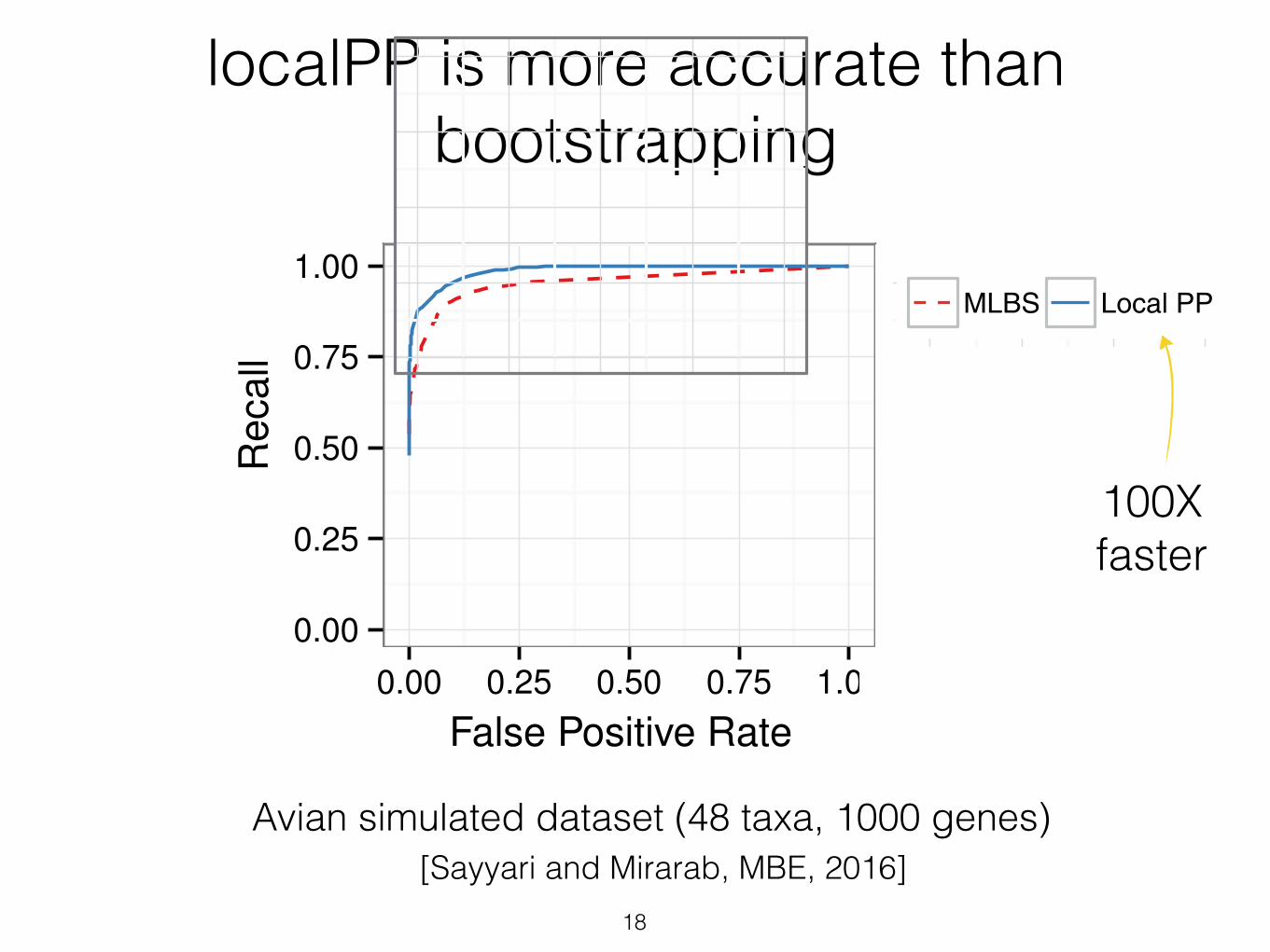
localPP is more accurate than bootstrapping
250 500
1000 1500
0.00
0.25
0.50
0.75
1.00
0.00
0.25
0.50
0.75
1.00
0.00 0.25 0.50 0.75 1.000.00 0.25 0.50 0.75 1.00
False Positive Rate
Recall
MLBS Local PP
250 500
1000 1500
0.00
0.25
0.50
0.75
1.00
0.00
0.25
0.50
0.75
1.00
0.00 0.25 0.50 0.75 1.000.00 0.25 0.50 0.75 1.00
False Positive Rate
Recall
MLBS Local PP
250 500
1000 1500
0.00
0.25
0.50
0.75
1.00
0.00
0.25
0.50
0.75
1.00
0.00 0.25 0.50 0.75 1.000.00 0.25 0.50 0.75 1.00
False Positive Rate
Recall
MLBS Local PP
250 500
1000 1500
0.00
0.25
0.50
0.75
1.00
0.00
0.25
0.50
0.75
1.00
0.00 0.25 0.50 0.75 1.000.00 0.25 0.50 0.75 1.00
False Positive Rate
Recall
MLBS Local PP
Avian simulated dataset (48 taxa, 1000 genes)
the ROC curves show (fig. 5), for the same number offalse positives branches, local posterior probabilities result inbetter recall than MLBS. This pattern is more pronouncedfor shorter alignments, which have increased gene treeerror. For example, for the 250 bp model condition, if wechoose a support threshold that results in 0.01 FPR, with localposterior values, we still recover 84% of correct branches,whereas with MLBS, the same FPR results in retaining70% of correct branches. Thus, for a desired level of precision,better recall can be obtained using local posteriorprobabilities.
Branch LengthBranch length accuracy on the avian dataset was a function ofgene tree estimation error whether ASTRAL or MP-EST wasused (table 4). With true gene trees, branch length log error
FIG. 4. Branch length accuracy on the A-200 dataset with Medium ILS. See supplementary figures S7 and S8, Supplementary Material online forlow and high ILS. The estimated branch length is plotted against the true branch length in log scale (base 10). Blue line: a fitted generalizedadditive model with smoothing (Wood 2011).
Table 3. Branch Length Accuracy on the A-200 Dataset.
Dataset n Log Err RMSE
True gt Est. gt True gt Est. gt
Low ILS 1,000 0.10 0.42 5.57 6.75Low ILS 200 0.16 0.44 6.22 6.99Low ILS 50 0.25 0.48 6.84 7.29Med ILS 1,000 0.03 0.20 0.22 0.86Med ILS 200 0.07 0.22 0.44 0.91Med ILS 50 0.13 0.26 0.74 1.05High ILS 1,000 0.06 0.15 0.03 0.13High ILS 200 0.11 0.18 0.07 0.15High ILS 50 0.18 0.24 0.14 0.19
NOTE.—Logarithmic error (Log Err) and RMSE are shown for true species treesscored with true gene trees or estimated gene trees (Est. gt).
250 500
1000 1500
0.00
0.25
0.50
0.75
1.00
0.00
0.25
0.50
0.75
1.00
0.00 0.25 0.50 0.75 1.000.00 0.25 0.50 0.75 1.00False Positive Rate
Rec
all
MLBS Local PP
FIG. 5. ROC curve for the avian dataset based on MLBS and local PPPPsupport values. Boxes show different numbers of sites per gene (con-trolling gene tree estimation error).
Fast Coalescent-Based Support Computation . doi:10.1093/molbev/msw079 MBE
9
by guest on May 28, 2016
http://mbe.oxfordjournals.org/
Dow
nloaded from
[Sayyari and Mirarab, MBE, 2016]
100Xfaster
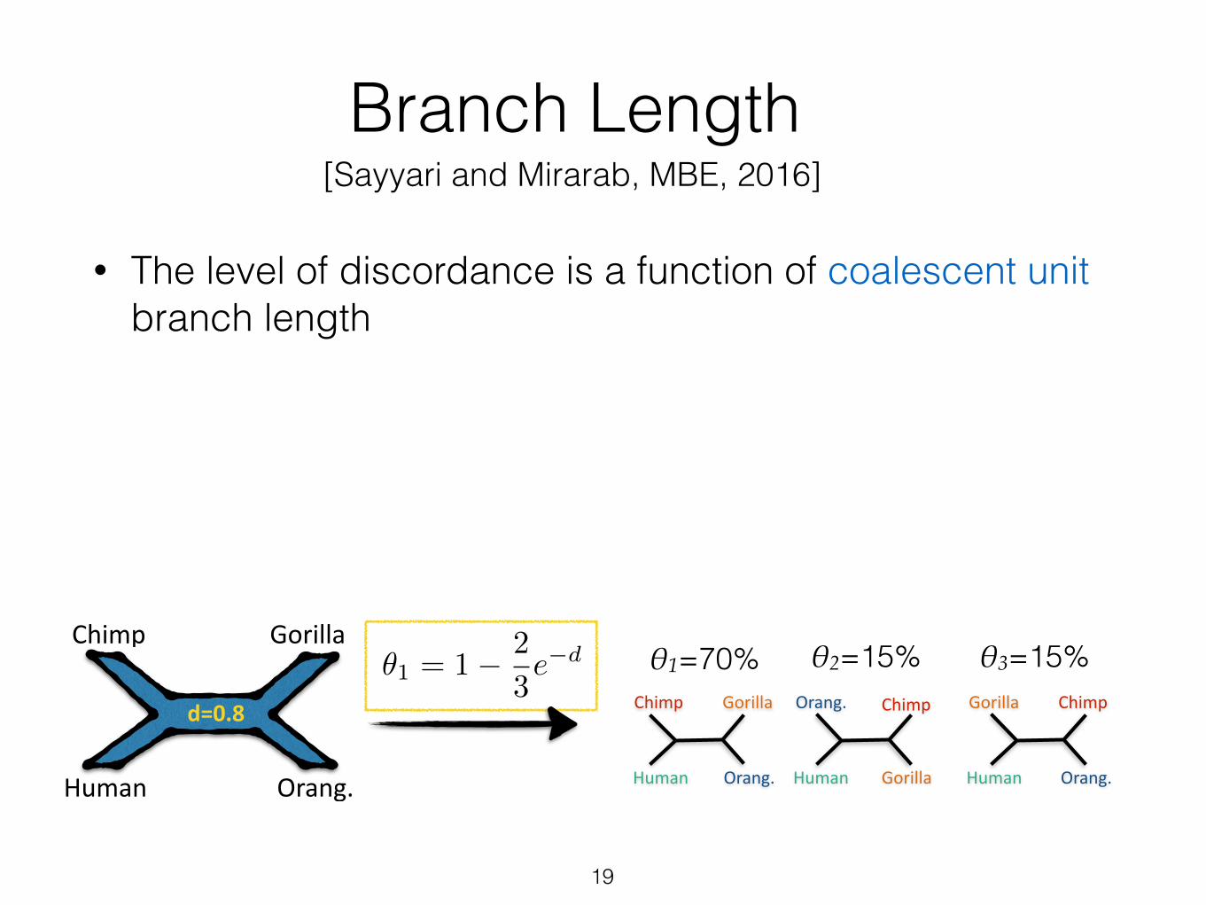
Branch Length
• The level of discordance is a function of coalescent unit branch length
19
[Sayyari and Mirarab, MBE, 2016]
Orang.
Gorilla Chimp
HumanOrang.
GorillaChimp
Human
Orang.
Gorilla
Chimp
Human
θ2=15% θ3=15%θ1=70%Gorilla
Orang.
Chimp
Human
d=0.8
✓1 = 1� 2
3e�d
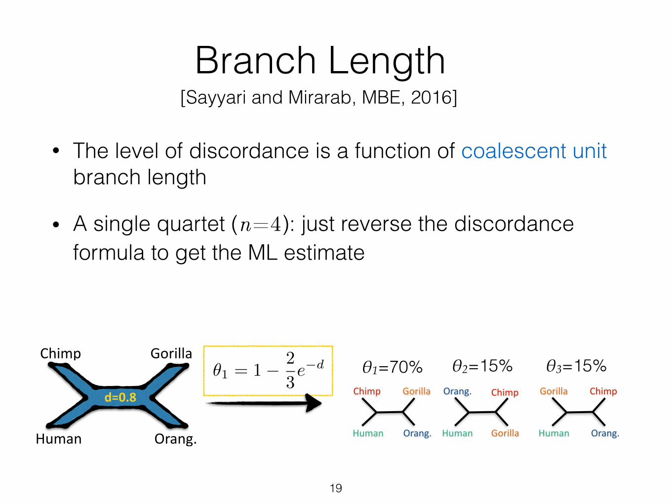
Branch Length
• The level of discordance is a function of coalescent unit branch length
• A single quartet (n=4): just reverse the discordance formula to get the ML estimate
19
[Sayyari and Mirarab, MBE, 2016]
Orang.
Gorilla Chimp
HumanOrang.
GorillaChimp
Human
Orang.
Gorilla
Chimp
Human
θ2=15% θ3=15%θ1=70%Gorilla
Orang.
Chimp
Human
d=0.8
✓1 = 1� 2
3e�d
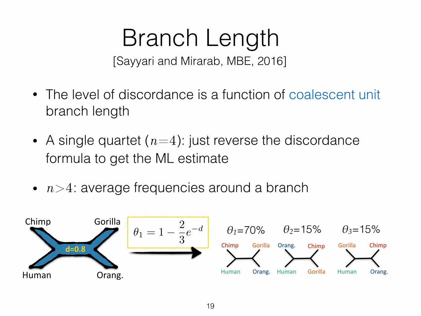
Branch Length
• The level of discordance is a function of coalescent unit branch length
• A single quartet (n=4): just reverse the discordance formula to get the ML estimate
• n>4: average frequencies around a branch
19
[Sayyari and Mirarab, MBE, 2016]
Orang.
Gorilla Chimp
HumanOrang.
GorillaChimp
Human
Orang.
Gorilla
Chimp
Human
θ2=15% θ3=15%θ1=70%Gorilla
Orang.
Chimp
Human
d=0.8
✓1 = 1� 2
3e�d
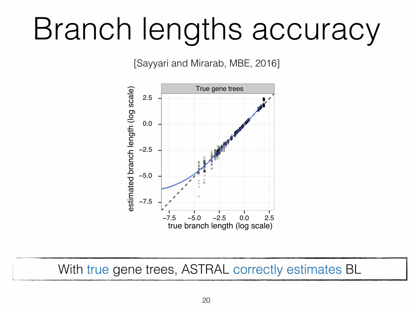
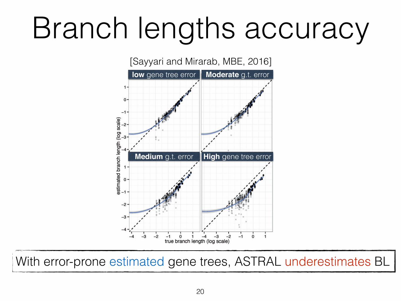
Branch lengths accuracy
20
True gene trees
1500 1000
500 250
−7.5
−5.0
−2.5
0.0
2.5
−7.5
−5.0
−2.5
0.0
2.5
−7.5 −5.0 −2.5 0.0 2.5 −7.5 −5.0 −2.5 0.0 2.5true branch length (log scale)
estim
ated
bra
nch
leng
th (l
og s
cale
)
−7.5
−5.0
−2.5
0.0
2.5
−7.5 −5.0 −2.5 0.0 2.5true branch length (log scale)
estim
ated
bra
nch
leng
th (l
og s
cale
)
With true gene trees, ASTRAL correctly estimates BL
[Sayyari and Mirarab, MBE, 2016]
Branch lengths accuracy
20
True gene trees
1500 1000
500 250
−7.5
−5.0
−2.5
0.0
2.5
−7.5
−5.0
−2.5
0.0
2.5
−7.5 −5.0 −2.5 0.0 2.5 −7.5 −5.0 −2.5 0.0 2.5true branch length (log scale)
estim
ated
bra
nch
leng
th (l
og s
cale
)
−7.5
−5.0
−2.5
0.0
2.5
−7.5 −5.0 −2.5 0.0 2.5true branch length (log scale)
estim
ated
bra
nch
leng
th (l
og s
cale
)
was only 0.06, corresponding to branches that are about 14%shorter or longer than the true branch. As gene tree estima-tion error increases with reduced number of sites (see table 1for gene tree error statistics), the branch length error also
increases. Thus, while 1,500 bp genes give 0.17 log error,250 bp genes result in 0.59 error, which corresponds tobranches that are on average 3.9 times too short or long.Moreover, unlike true gene trees, the error in branch lengthsestimated based on estimated gene trees is biased towardunderestimation (fig. 6), a pattern that increases in intensitywith shorter alignments.
ASTRAL and MP-EST have similar branch length accuracymeasured by log error for highly accurate gene trees, butASTRAL has an advantage with increased gene tree error(supplementary fig. S10, Supplementary Material online andtable 4). Error measured by root mean squared error (RMSE)(which emphasizes the accuracy of long branches) is compa-rable for the two methods, but MP-EST has a slight advantagegiven accurate gene trees.
Biological DatasetsFor each biological dataset, we show MLBS support and thelocal posterior probabilities, computed based on RAxML genetrees available from respective publications. We also collapsegene tree branches with <33% bootstrap support and usethese collapsed gene trees to draw local posterior probabili-ties. For ease of discussion, we show local posterior probabil-ities as percentages and refer to them simply as posterior orcollapsed posterior (for values based on collapsed gene trees).We discuss the confidence in important branches in eachtree.
1KP. Three of the key relationships studied by Wickett et al.(2014) are the sister branch to land plants, the base of theangiosperms, and the relationship among Bryophytes (horn-worts, liverworts, and mosses). In the ASTRAL tree, manybranches have full support regardless of the measure of thesupport used, but the remaining branches reveal interestingpatterns (fig. 7). The sister relationship betweenZygnematales and land plants receives a moderate 80% BS,but has 100% posterior. Wickett et al. (2014) also recoveredthis relationship by concatenation of various data partitions.There are 12 other branches that have collapsed posteriorsthat are at least 10% higher than BS (fig. 7); no branch hassubstantially higher BS than collapsed posterior. Collapsedposterior for monophyly of Bryophytes and for Amborellaas sister to other angiosperms are 100% (compared with97% and 93% BS, respectively).
When we collapse low-support branches in gene trees,posterior goes up for several branches: nine branches haveimprovements of 10% or more, and only two branches havecomparable reductions. An interesting case is Coleochaetalesas sister to Zygnematalesþ land plants, which has only 62%BS and 61% posterior, but has 100% collapsed posterior.Finally, note that several branches have low posterior, evenafter collapsing.
Our estimated branch lengths are short for several nodes.For example, the branch that unites (ChloranthalesþMagnoliids) and Eudicots has a length of 0.14 in coalescentunits. Other branches that have been historically hard to re-cover also tend to have short branches; however, these arenot necessarily extremely short branches that would
FIG. 6. ASTRAL branch length accuracy on the avian dataset. Logtransformed estimated branch lengths are shown versus true branchlengths, and a generalized additive model is fitted to the data. Onebranch with length 10"6 is trimmed out here, but full results, includ-ing MP-EST, is shown in supplementary figure S9, SupplementaryMaterial online.
Table 4. Branch Length Accuracy for the Avian Dataset.
No. of sites Log Err RMSE
ASTRAL MPEST ASTRAL MPEST
True gt. 0.06 (0.10) 0.07 (0.11) 0.44 (0.44) 0.30 (0.30)1,500 0.17 (0.20) 0.14 (0.18) 0.83 (0.83) 0.70 (0.70)1,000 0.22 (0.27) 0.22 (0.25) 1.08 (1.07) 1.01 (1.00)500 0.37 (0.42) 0.42 (0.46) 1.65 (1.64) 1.65 (1.64)250 0.59 (0.63) 0.81 (0.84) 2.25 (2.24) 2.28 (2.26)
NOTE.—Logarithmic error and root mean squared error are shown for true speciestrees scored with true gene trees or estimated gene trees with various numbers ofsites using ASTRAL and MP-EST. An extremely short branch with length 10"6 wasremoved from the calculations, but error including that branch is shownparenthetically.
Sayyari and Mirarab . doi:10.1093/molbev/msw079 MBE
10
by guest on May 28, 2016
http://mbe.oxfordjournals.org/
Dow
nloaded from
low gene tree error
High gene tree error
Moderate g.t. error
Medium g.t. error
With true gene trees, ASTRAL correctly estimates BLWith error-prone estimated gene trees, ASTRAL underestimates BL
[Sayyari and Mirarab, MBE, 2016]
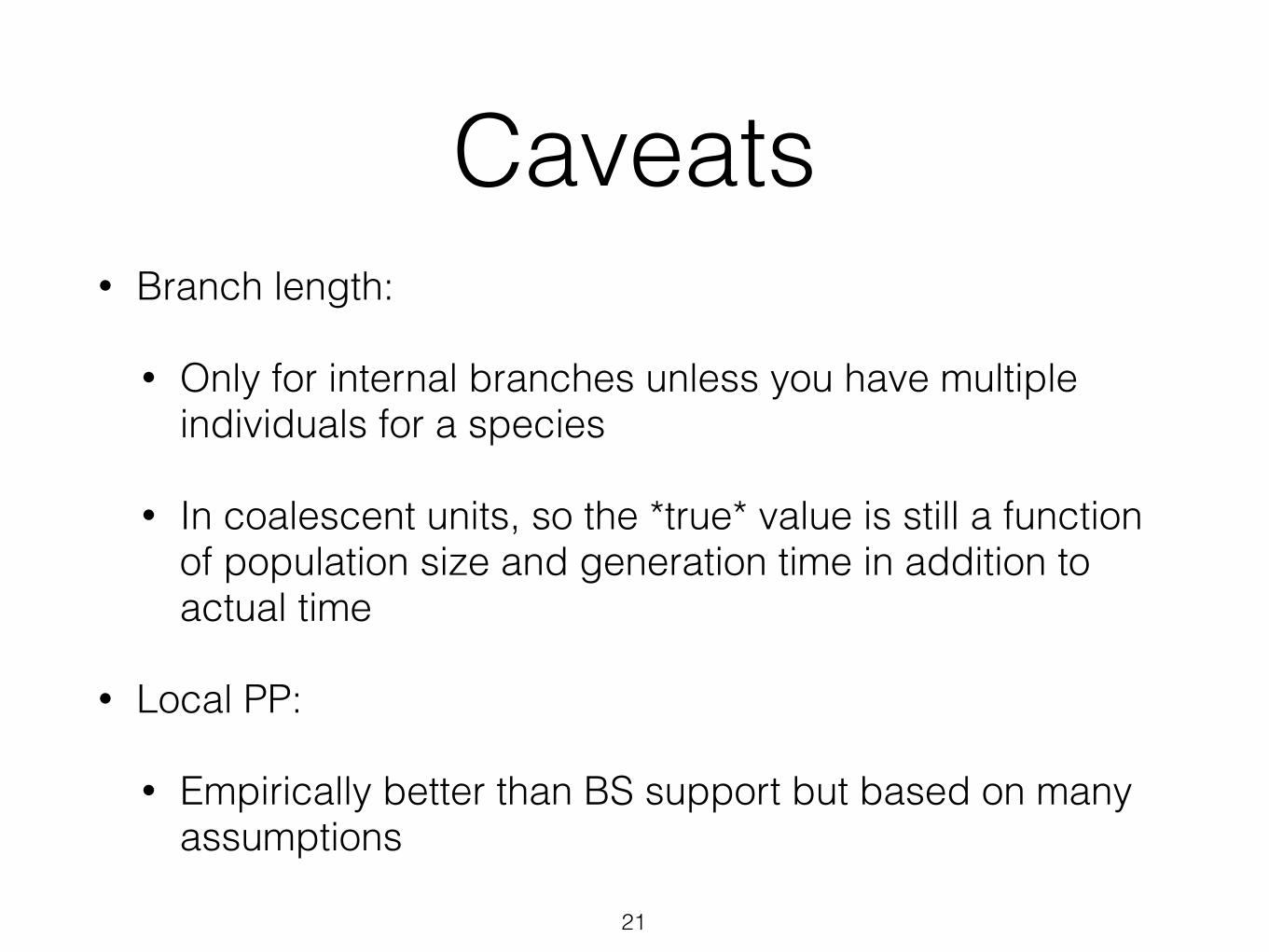
Caveats• Branch length:
• Only for internal branches unless you have multiple individuals for a species
• In coalescent units, so the *true* value is still a function of population size and generation time in addition to actual time
• Local PP:
• Empirically better than BS support but based on many assumptions
21

Examples
22
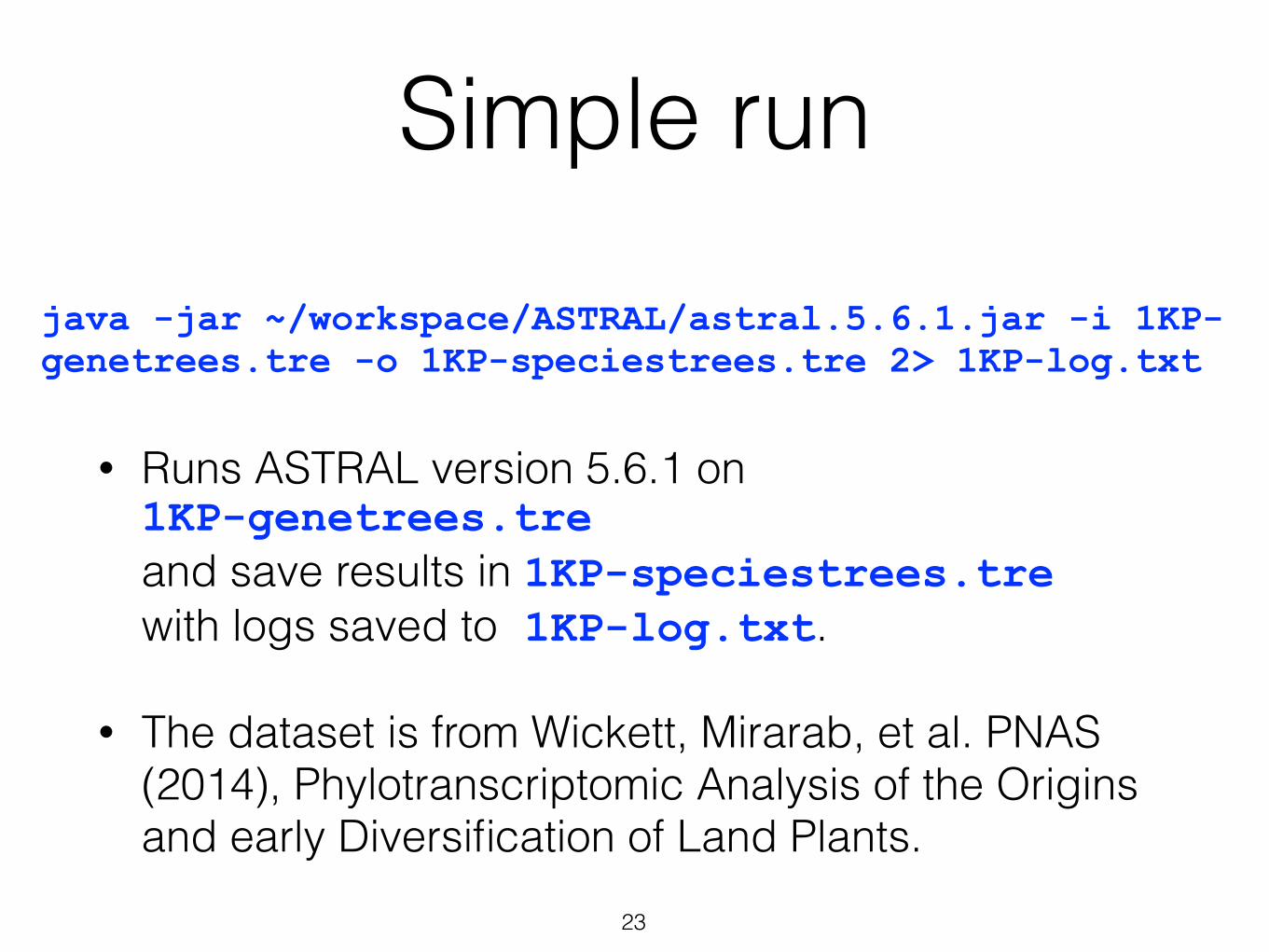
Simple run
• Runs ASTRAL version 5.6.1 on 1KP-genetrees.tre and save results in 1KP-speciestrees.tre with logs saved to 1KP-log.txt.
• The dataset is from Wickett, Mirarab, et al. PNAS (2014), Phylotranscriptomic Analysis of the Origins and early Diversification of Land Plants.
23
java -jar ~/workspace/ASTRAL/astral.5.6.1.jar -i 1KP-genetrees.tre -o 1KP-speciestrees.tre 2> 1KP-log.txt
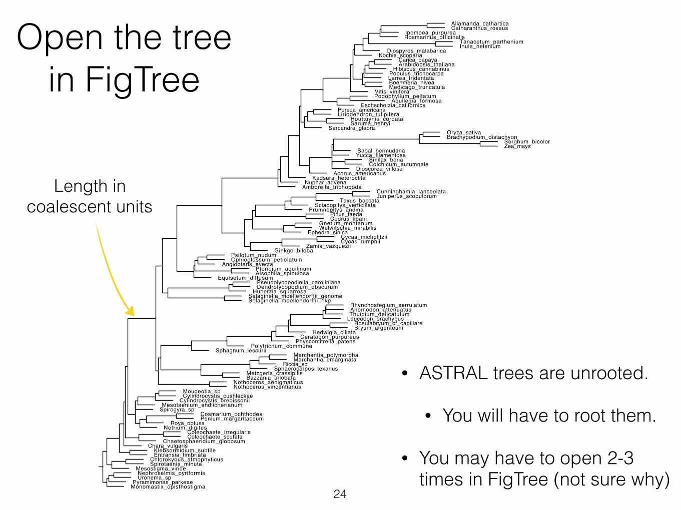
Open the tree in FigTree
• ASTRAL trees are unrooted.
• You will have to root them.
• You may have to open 2-3 times in FigTree (not sure why)
24
Equisetum_diffusum
Bazzania_trilobata
Rhynchostegium_serrulatum
Riccia_sp
Hibiscus_cannabinus
Bryum_argenteum
Juniperus_scopulorum
Vitis_vinifera
Eschscholzia_californicaPodophyllum_peltatum
Physcomitrella_patens
Mesostigma_viride
Rosulabryum_cf_capillare
Prumnopitys_andina
Acorus_americanus
Selaginella_moellendorffii_1kp
Carica_papaya
Roya_obtusa
Chlorokybus_atmophyticus
Spirogyra_sp
Sorghum_bicolor
Thuidium_delicatulum
Sciadopitys_verticillata
Pseudolycopodiella_caroliniana
Taxus_baccata
Sarcandra_glabra
Boehmeria_nivea
Persea_americana
Catharanthus_roseus
Arabidopsis_thaliana
Nuphar_advena
Spirotaenia_minuta
Cycas_rumphii
Penium_margaritaceum
Dioscorea_villosa
Cycas_micholitzii
Kadsura_heteroclita
Sphagnum_lescurii
Ceratodon_purpureus
Aquilegia_formosa
Angiopteris_evecta
Coleochaete_irregularis
Kochia_scoparia
Cunninghamia_lanceolata
Netrium_digitus
Marchantia_polymorpha
Inula_helenium
Nothoceros_aenigmaticus
Ipomoea_purpurea
Yucca_filamentosa
Cylindrocystis_cushleckae
Gnetum_montanum
Metzgeria_crassipilis
Ginkgo_bilobaPsilotum_nudum
Dendrolycopodium_obscurum
Monomastix_opisthostigma
Liriodendron_tulipifera
Mougeotia_sp
Mesotaenium_endlicherianum
Diospyros_malabarica
Ephedra_sinica
Allamanda_cathartica
Zamia_vazquezii
Rosmarinus_officinalis
Saruma_henryi
Pteridium_aquilinum
Sphaerocarpos_texanus
Klebsormidium_subtile
Colchicum_autumnale
Amborella_trichopoda
Pinus_taeda
Leucodon_brachypus
Pyramimonas_parkeae
Sabal_bermudana
Cosmarium_ochthodes
Chaetosphaeridium_globosum
Huperzia_squarrosa
Zea_mays
Chara_vulgaris
Medicago_truncatula
Nephroselmis_pyriformis
Tanacetum_parthenium
Alsophila_spinulosa
Populus_trichocarpa
Cedrus_libani
Anomodon_attenuatus
Oryza_sativa
Marchantia_emarginata
Brachypodium_distachyon
Cylindrocystis_brebissonii
Uronema_sp
Entransia_fimbriata
Nothoceros_vincentianus
Smilax_bona
Larrea_tridentata
Polytrichum_commune
Coleochaete_scutata
Selaginella_moellendorffii_genome
Welwitschia_mirabilis
Ophioglossum_petiolatum
Houttuynia_cordata
Hedwigia_ciliata
Length in coalescent units
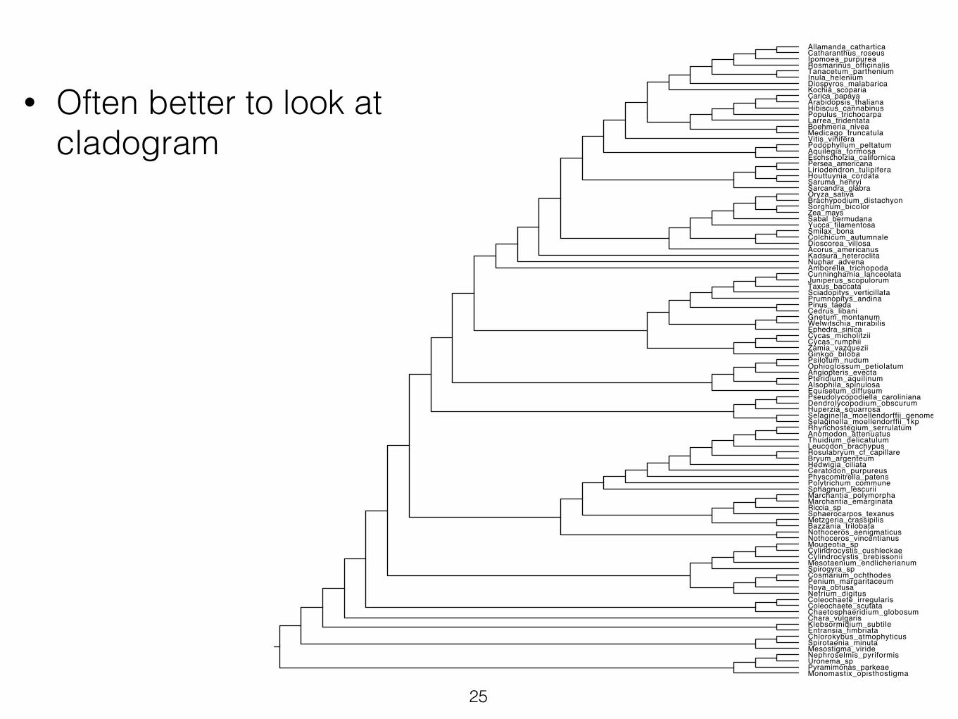
• Often better to look at cladogram
25
Entransia_fimbriata
Smilax_bona
Mougeotia_sp
Klebsormidium_subtile
Angiopteris_evecta
Marchantia_emarginata
Pinus_taedaCedrus_libani
Acorus_americanus
Psilotum_nudum
Eschscholzia_californica
Ophioglossum_petiolatum
Hibiscus_cannabinus
Sarcandra_glabra
Amborella_trichopoda
Catharanthus_roseus
Cylindrocystis_brebissonii
Oryza_sativa
Bazzania_trilobata
Uronema_sp
Chlorokybus_atmophyticus
Pyramimonas_parkeae
Brachypodium_distachyon
Houttuynia_cordata
Carica_papaya
Populus_trichocarpa
Dioscorea_villosa
Ephedra_sinica
Selaginella_moellendorffii_1kp
Diospyros_malabarica
Cylindrocystis_cushleckaeMesotaenium_endlicherianum
Coleochaete_scutata
Pteridium_aquilinum
Sorghum_bicolor
Cycas_micholitzii
Chara_vulgaris
Cycas_rumphii
Nuphar_advena
Arabidopsis_thaliana
Prumnopitys_andina
Pseudolycopodiella_caroliniana
Nephroselmis_pyriformis
Metzgeria_crassipilis
Aquilegia_formosa
Riccia_sp
Chaetosphaeridium_globosum
Physcomitrella_patens
Vitis_vinifera
Leucodon_brachypus
Roya_obtusa
Sciadopitys_verticillata
Larrea_tridentata
Equisetum_diffusum
Penium_margaritaceum
Sphaerocarpos_texanus
Zea_mays
Liriodendron_tulipifera
Marchantia_polymorpha
Ipomoea_purpurea
Sabal_bermudana
Rosulabryum_cf_capillare
Medicago_truncatula
Dendrolycopodium_obscurum
Ceratodon_purpureus
Allamanda_cathartica
Selaginella_moellendorffii_genome
Yucca_filamentosa
Saruma_henryi
Mesostigma_viride
Podophyllum_peltatum
Thuidium_delicatulum
Inula_heleniumRosmarinus_officinalis
Welwitschia_mirabilis
Spirogyra_sp
Colchicum_autumnale
Cosmarium_ochthodes
Kadsura_heteroclita
Coleochaete_irregularis
Rhynchostegium_serrulatum
Monomastix_opisthostigma
Taxus_baccata
Gnetum_montanum
Persea_americana
Alsophila_spinulosa
Sphagnum_lescurii
Cunninghamia_lanceolata
Netrium_digitus
Spirotaenia_minuta
Kochia_scoparia
Huperzia_squarrosa
Juniperus_scopulorum
Polytrichum_commune
Zamia_vazquezii
Nothoceros_vincentianus
Tanacetum_parthenium
Ginkgo_biloba
Boehmeria_nivea
Hedwigia_ciliata
Nothoceros_aenigmaticus
Anomodon_attenuatus
Bryum_argenteum
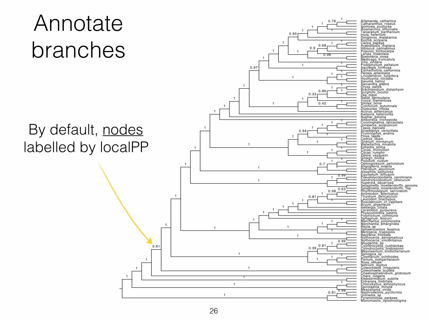
Annotate branches
26
Entransia_fimbriata
Smilax_bona
Mougeotia_sp
Klebsormidium_subtile
Angiopteris_evecta
Marchantia_emarginata
Pinus_taedaCedrus_libani
Acorus_americanus
Psilotum_nudum
Eschscholzia_californica
Ophioglossum_petiolatum
Hibiscus_cannabinus
Sarcandra_glabra
Amborella_trichopoda
Catharanthus_roseus
Cylindrocystis_brebissonii
Oryza_sativa
Bazzania_trilobata
Uronema_sp
Chlorokybus_atmophyticus
Pyramimonas_parkeae
Brachypodium_distachyon
Houttuynia_cordata
Carica_papaya
Populus_trichocarpa
Dioscorea_villosa
Ephedra_sinica
Selaginella_moellendorffii_1kp
Diospyros_malabarica
Cylindrocystis_cushleckaeMesotaenium_endlicherianum
Coleochaete_scutata
Pteridium_aquilinum
Sorghum_bicolor
Cycas_micholitzii
Chara_vulgaris
Cycas_rumphii
Nuphar_advena
Arabidopsis_thaliana
Prumnopitys_andina
Pseudolycopodiella_caroliniana
Nephroselmis_pyriformis
Metzgeria_crassipilis
Aquilegia_formosa
Riccia_sp
Chaetosphaeridium_globosum
Physcomitrella_patens
Vitis_vinifera
Leucodon_brachypus
Roya_obtusa
Sciadopitys_verticillata
Larrea_tridentata
Equisetum_diffusum
Penium_margaritaceum
Sphaerocarpos_texanus
Zea_mays
Liriodendron_tulipifera
Marchantia_polymorpha
Ipomoea_purpurea
Sabal_bermudana
Rosulabryum_cf_capillare
Medicago_truncatula
Dendrolycopodium_obscurum
Ceratodon_purpureus
Allamanda_cathartica
Selaginella_moellendorffii_genome
Yucca_filamentosa
Saruma_henryi
Mesostigma_viride
Podophyllum_peltatum
Thuidium_delicatulum
Inula_heleniumRosmarinus_officinalis
Welwitschia_mirabilis
Spirogyra_sp
Colchicum_autumnale
Cosmarium_ochthodes
Kadsura_heteroclita
Coleochaete_irregularis
Rhynchostegium_serrulatum
Monomastix_opisthostigma
Taxus_baccata
Gnetum_montanum
Persea_americana
Alsophila_spinulosa
Sphagnum_lescurii
Cunninghamia_lanceolata
Netrium_digitus
Spirotaenia_minuta
Kochia_scoparia
Huperzia_squarrosa
Juniperus_scopulorum
Polytrichum_commune
Zamia_vazquezii
Nothoceros_vincentianus
Tanacetum_parthenium
Ginkgo_biloba
Boehmeria_nivea
Hedwigia_ciliata
Nothoceros_aenigmaticus
Anomodon_attenuatus
Bryum_argenteum
1
1
1
1
1
1
1
0.94
1
1
1
1
1
0.99
1
1
1
1
1
1
1
1
1
0.7
0.39
1
0.63
0.81
1
1
0.61
1
0.68
1
11
1
1
1
1
1
1
0.98
1
1
1
1
0.42
1
1
1
1
1
1
1
1
0.98
0.86
1
1
1
1
1
1
1
1 1
1
1
1
1
1
0.76
1
0.81
1
1
0.9
0.81
1
1
1
0.98
0.97
1
1
1
1
1
1
1
1
1
11
0.99
1
0.95
0.331
1
By default, nodes labelled by localPP
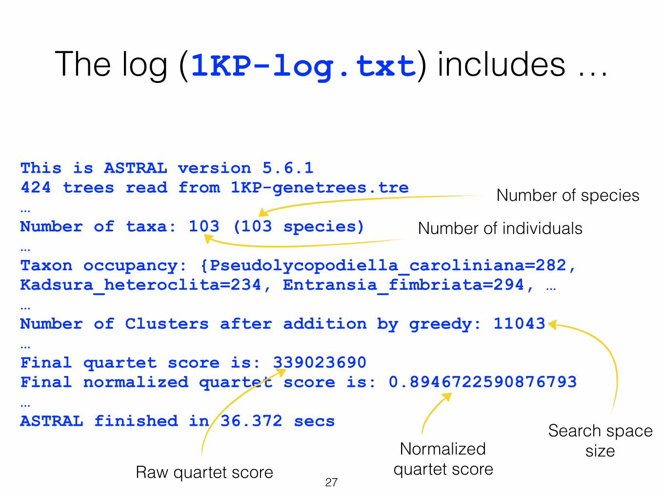
The log (1KP-log.txt) includes …
27
This is ASTRAL version 5.6.1 424 trees read from 1KP-genetrees.tre … Number of taxa: 103 (103 species) … Taxon occupancy: {Pseudolycopodiella_caroliniana=282, Kadsura_heteroclita=234, Entransia_fimbriata=294, … … Number of Clusters after addition by greedy: 11043 … Final quartet score is: 339023690 Final normalized quartet score is: 0.8946722590876793 … ASTRAL finished in 36.372 secs
Number of individuals
Number of species
Search space sizeNormalized
quartet scoreRaw quartet score
Main publications• Mirarab, Siavash, Rezwana Reaz, Md. Shamsuzzoha Bayzid, Théo
Zimmermann, M. S. Swenson, and Tandy Warnow. “ASTRAL: Genome-Scale Coalescent-Based Species Tree Estimation.” Bioinformatics 30, no. 17 (2014): i541–48. https://doi.org/10.1093/bioinformatics/btu462.
• Mirarab, S., and T. Warnow. “ASTRAL-II: Coalescent-Based Species Tree Estimation with Many Hundreds of Taxa and Thousands of Genes.” Bioinformatics 31, no. 12 (2015). https://doi.org/10.1093/bioinformatics/btv234.
• Zhang, Chao, Maryam Rabiee, Erfan Sayyari, and Siavash Mirarab. “ASTRAL-III: Polynomial Time Species Tree Reconstruction from Partially Resolved Gene Trees.” BMC Bioinformatics 19, no. S6 (2018): 153. https://doi.org/10.1186/s12859-018-2129-y.
• Sayyari, Erfan, and Siavash Mirarab. “Fast Coalescent-Based Computation of Local Branch Support from Quartet Frequencies.” Molecular Biology and Evolution 33, no. 7 (2016): 1654–68. https://doi.org/10.1093/molbev/msw079.
28
Some other ASTRAL-related papers• Testing for polytomies in species trees using quartet frequencies (Sayyari and Mirarab).
Genes (2018) (Note: Implemented in option -t 10)
• Filtering loci is not beneficial! (Molloy and Warnow), Systematic Biology (2018)
• ASTRAL consistent under models of missing data (Nute, Molloy, Chou, and Warnow). BMC Genomics (2018)
• SIESTA improves ASTRAL (Vachaspati and Warnow). BMC Genomics (2018)
• Visualizing Discordance using DiscoVista (Sayyari, Whitfield, and Mirarab). Molecular Phylogenetics and Evolution (2018)
• Fragmentary sequences can negatively impact ASTRAL trees (Sayyari, Whitfield, and Mirarab). Molecular Biology and Evolution (2017)
• How many genes does ASTRAL need? (Shekhar, Roch, and Mirarab). Transactions on Computational Biology and Bioinformatics (2017)
• Using ASTRAL as a supertree method (Vachaspati and Warnow). Bioinformatics (2017)
• Performance under ILS and HGT (Davidson, Vachaspati, Mirarab, and Warnow). BMC Genomics (2015).
29
For more info• Contact me: Tandy Warnow, [email protected]
• Main developer: Siavash Mirarab, [email protected]
• Software available at Github site: https://github.com/smirarab/ASTRAL
• See tutorial and README at GitHub site: https://github.com/smirarab/ASTRAL/blob/master/astral-tutorial.md
• Email: [email protected]
• More related papers at http://tandy.cs.illinois.edu/papers-all.html and http://eceweb.ucsd.edu/~smirarab/publications.html
• Related software (ASTRID, SVDquest, FastRFS, SIESTA) on github, and linked from http://tandy.cs.illinois.edu/software.html. See also https://github.com/esayyari/DiscoVista for DiscoVista.
30
Phylogenomics Software Symposium
• Location: ISEM, Montpellier, France on August 17, 2018
• Travel awards available for up to $500 per person
• Tutorial on phylogenomics provided by Siavash Mirarab
• Research talks by Mirarab, Nakhleh, Kosiol, Tannier, Warnow (and other contributed talks)
• Free - no fee, but registration required (limited to 50 people)
• See http://tandy.cs.illinois.edu/PhyloSynth-Symposium.html for more information
31
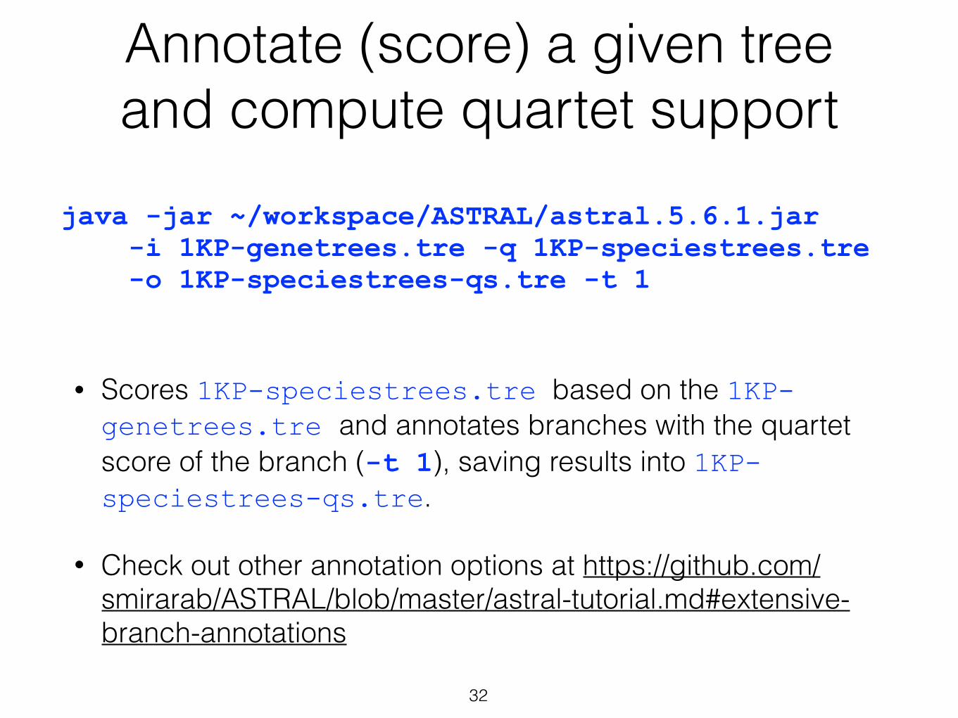
Annotate (score) a given tree and compute quartet support
• Scores 1KP-speciestrees.tre based on the 1KP-genetrees.tre and annotates branches with the quartet score of the branch (-t 1), saving results into 1KP-speciestrees-qs.tre.
• Check out other annotation options at https://github.com/smirarab/ASTRAL/blob/master/astral-tutorial.md#extensive-branch-annotations
32
java -jar ~/workspace/ASTRAL/astral.5.6.1.jar -i 1KP-genetrees.tre -q 1KP-speciestrees.tre -o 1KP-speciestrees-qs.tre -t 1
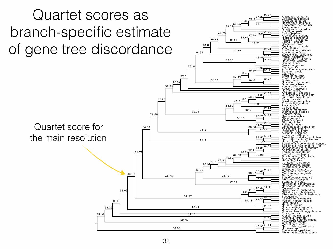
Quartet scores as branch-specific estimate of gene tree discordance
33
Quartet score for the main resolution
Brachypodium_distachyon
Alsophila_spinulosa
Selaginella_moellendorffii_genome
Eschscholzia_californica
Riccia_sp
Ophioglossum_petiolatum
Kochia_scoparia
Ephedra_sinica
Sarcandra_glabra
Nephroselmis_pyriformis
Cycas_micholitzii
Liriodendron_tulipifera
Zamia_vazquezii
Chlorokybus_atmophyticus
Smilax_bona
Nothoceros_aenigmaticus
Pseudolycopodiella_caroliniana
Entransia_fimbriata
Marchantia_emarginata
Persea_americana
Sphaerocarpos_texanus
Ipomoea_purpurea
Chara_vulgaris
Nothoceros_vincentianus
Marchantia_polymorpha
Welwitschia_mirabilis
Mougeotia_sp
Podophyllum_peltatum
Taxus_baccata
Cylindrocystis_brebissoniiSpirogyra_sp
Rhynchostegium_serrulatum
Rosulabryum_cf_capillare
Physcomitrella_patens
Larrea_tridentata
Sciadopitys_verticillata
Cosmarium_ochthodesPenium_margaritaceum
Coleochaete_irregularis
Sorghum_bicolor
Ceratodon_purpureus
Ginkgo_biloba
Medicago_truncatula
Houttuynia_cordata
Gnetum_montanum
Metzgeria_crassipilis
Rosmarinus_officinalis
Nuphar_advena
Uronema_sp
Cedrus_libani
Mesotaenium_endlicherianum
Acorus_americanus
Catharanthus_roseus
Hedwigia_ciliataBryum_argenteum
Chaetosphaeridium_globosum
Sabal_bermudana
Cycas_rumphii
Kadsura_heteroclita
Equisetum_diffusum
Netrium_digitus
Cylindrocystis_cushleckae
Inula_helenium
Selaginella_moellendorffii_1kp
Polytrichum_commune
Populus_trichocarpa
Angiopteris_evecta
Roya_obtusa
Tanacetum_parthenium
Colchicum_autumnale
Monomastix_opisthostigma
Psilotum_nudum
Allamanda_cathartica
Diospyros_malabarica
Boehmeria_niveaVitis_vinifera
Sphagnum_lescurii
Coleochaete_scutata
Pinus_taeda
Bazzania_trilobata
Prumnopitys_andina
Carica_papaya
Anomodon_attenuatus
Dendrolycopodium_obscurum
Thuidium_delicatulum
Mesostigma_viride
Dioscorea_villosa
Aquilegia_formosa
Hibiscus_cannabinus
Spirotaenia_minuta
Zea_mays
Pteridium_aquilinum
Huperzia_squarrosa
Arabidopsis_thaliana
Amborella_trichopoda
Oryza_sativa
Juniperus_scopulorum
Saruma_henryi
Yucca_filamentosa
Leucodon_brachypus
Klebsormidium_subtile
Cunninghamia_lanceolata
Pyramimonas_parkeae
48.11
70.41
37.78
55.64
90.25
65.36
87.08
64.57
95.51
51.6
36.96
86.81
75.2
92.65
57.27
72.05
67.74
51.14
82.35
34.03
49.47
92.72
61.25
43.33
40.24
37.22
98.52
33.4898.4
34.3
95.77
69.74
45.03
70.15
76.64
93.95
43.26
58.96
96.9
45.5
42.97
93.18
78.39
98.12
50.75
41.94
91.86
67.53
93.79
58.95
49.52
38.95
99.97
89.7
66.4
39.62
41.88
82.16
71.69
58.96
84.83
47.94
51.89
51.75
96.57
39.25
36.52
81.83
57.51
58.89
95.29
99.11
97.73
90.51
46.9
54.59
64.15
68.29
42.25
41.61
38.67
90.38
43.86
60.47
88.99
88.19
97.39
53.11
81.34
45.5
62.82
84.47
53.71
53.04
38.09
43.5
40.93
62.11
69.27
46.05
42.53
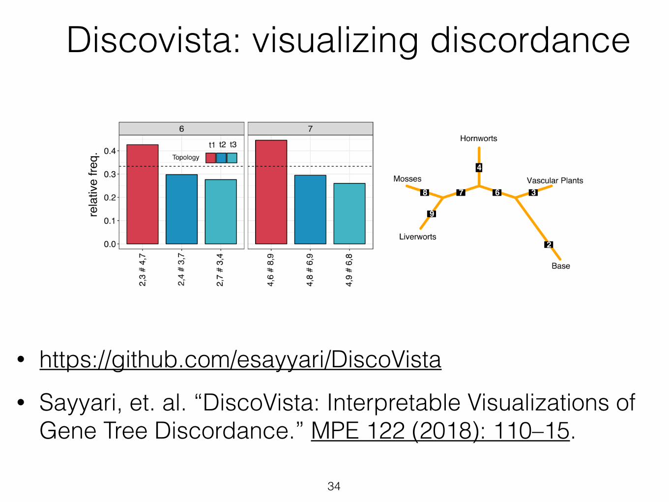
• https://github.com/esayyari/DiscoVista • Sayyari, et. al. “DiscoVista: Interpretable Visualizations of
Gene Tree Discordance.” MPE 122 (2018): 110–15.
34
Discovista: visualizing discordance
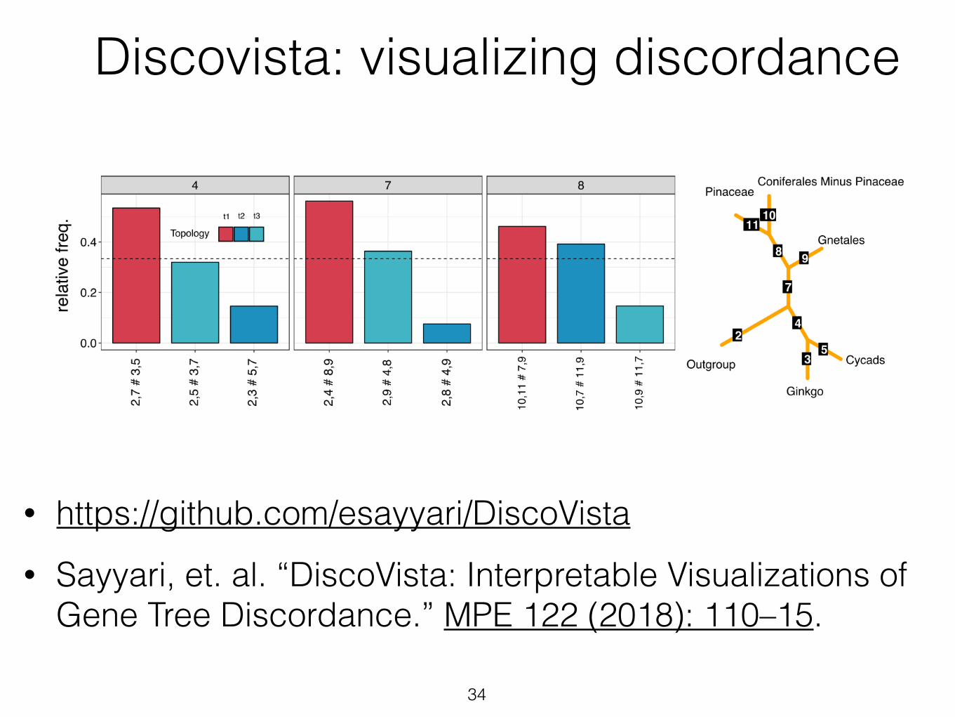
• https://github.com/esayyari/DiscoVista • Sayyari, et. al. “DiscoVista: Interpretable Visualizations of
Gene Tree Discordance.” MPE 122 (2018): 110–15.
34
Discovista: visualizing discordance
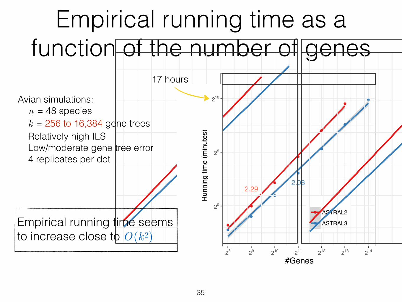
Empirical running time as a function of the number of genes
35
Zhang et al. Page 13 of 34
●
●
●
●
●
●
●
●
●
●
●
●
●
2.272.09
●
●
●
●
●
●
●
●
●
●
●
●
●
2.292.06
500 1500
28 29 210 211 212 213 214 28 29 210 211 212 213 214
20
25
210
#Genes
Run
ning
tim
e (m
inut
es)
●
●
ASTRAL2
ASTRAL3
Figure 5 Running time versus k. Average running times (4 replicates) are shown for ASTRAL-IIand ASTRAL-III on the avian dataset with 500bp or 1500bp alignments with varying numbers ofgens (k), shown in log scale (see Fig. S2 for normal scale). A line is fit to the data points in thelog/log space and line slopes are shown. ASTRAL-II did not finish on 214 genes in 48 hour.
branches has minimal impact on the discordance (eight discordant branches with
binned MP-EST instead of nine). However, contracting low support branches with
3%–33% thresholds dramatically reduces the discordance with the reference tree (2,
2, 4, 2, 3, and 3 discordant branches, respectively, for 3%, 5%, 7%, 10%, 20%, and
33%). Three thresholds (3%, 5%, and 10%) produce an identical tree (Fig. 4d). The
remaining di↵erences are among the branches that are deemed unresolved by Jarvis
et al. and change among the reference trees as well [5]. Contracting at 50% and 75%
thresholds, however, increases discordance to five and six branches, respectively.
Thus, consistent with simulations, contracting very low support branches seems
to produce the best results, when judged by similarity with the reference trees. To
summarize, ASTRAL-III obtained on unbinned but collapsed gene trees agreed with
all major relations in Jarvis et al., including the novel Columbea group, whereas
the unresolved tree missed important clades (Fig. 4).
3.2 RQ2: Running time improvements
We study the improvements in running time as various parameters change.
3.2.1 Varying the number of genes (k)
We compare ASTRAL-III to ASTRAL-II on the avian simulated dataset, changing
the number of genes from 28 to 214 and forcing X to be the same for both versions to
enable comparing impacts of improved weight calculation. We allow each replicate
run to take up to two days. ASTRAL-II is not able to finish on the dataset with
k = 214, while ASTRAL-III finishes on all conditions. ASTRAL-III improves the
running time over ASTRAL-II and the extent of the improvement depends on k
(Fig. 5). With 1000 genes or more, there is at least a 2.1X improvement. With
213 genes, the largest value where both versions could run, ASTRAL-III finishes
on average 3.2 times faster than ASTRAL-II (234 versus 758 minutes). Moreover,
fitting a line to the average running time in the log-log scale graph reveals that
on this dataset, the running time of ASTRAL-III on average grows as O(k2.08),
which is better than that of ASTRAL-II at O(k2.28), and both are better than the
theoretical worst case, which is O(k2.726).
Avian simulations: n = 48 species k = 256 to 16,384 gene trees Relatively high ILS Low/moderate gene tree error 4 replicates per dot
Empirical running time seems to increase close to O(k2)
17 hours
36
Zhang et al. Page 34 of 34
●
● ●
● ●
●
1.09
10k
20k
50k
100k
200k
500k
1M
200 500 1000 2000 5000 10000#Species
Size
of X
●
●
●
●
●
●
1.83
1
10
100
1000
200 500 1000 2000 5000 10000#Species
Run
ning
tim
e (m
inut
es)
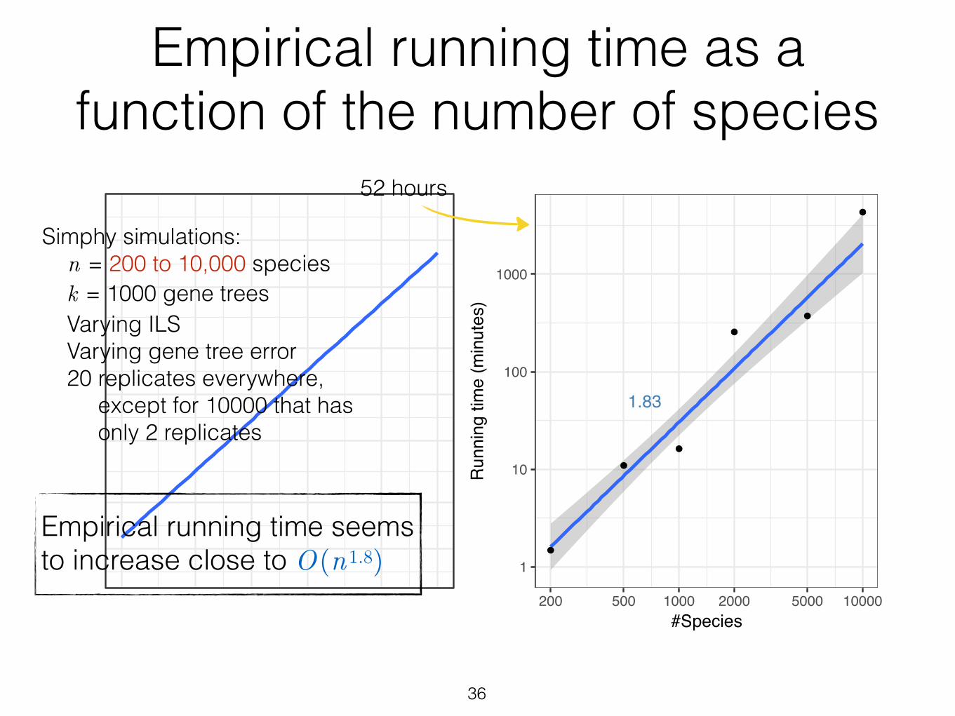
Figure S8 Empirical running time of ASTRAL-III with n. Average running time is shown forASTRAL-III for datasets with varying n. Averages are over 20 replicates. One replicate of 2000species dataset could not finish in 2 days and is removed from the analysis. Note that thesedatasets have factors other than n that change as well (e.g., the amount of ILS, etc.). Thus, theserunning times should be treated as ball-park estimates. Finally, we note that on the 10,000dataset, we have only 2 replicates and not 20.
Empirical running time as a function of the number of species
Empirical running time seems to increase close to O(n1.8)
Simphy simulations: n = 200 to 10,000 species k = 1000 gene trees Varying ILS Varying gene tree error 20 replicates everywhere, except for 10000 that has only 2 replicates
52 hours