Mark E. Sorrells

Genomic Selection:

A Step Change in Plant Breeding

People who contributed to research in this presentation • Jean-Luc Jannink – USDA/ARS, Cornell University

• Elliot Heffner – Pioneer Hi-Bred International

• Nicolas Heslot – Ph.D. Student, Cornell University

• Jessica Rutkoski - Ph.D. Student, Cornell University

• Julie Dawson – Post doc, Cornell University

• Jeff Endelman – Post doc, Cornell University

Presentation Overview

Genomic (Genome-Wide) Selection

• Characterizing GxE using marker effects

• Integration in a breeding program

• Biparental and Multi-Family predictions

• Recurrent Genomic Selection

Molecular Breeding Goals

• Allele discovery

• Allele characterization & validation

• Parental & progeny selection for superior alleles at multiple

loci to generate transgressive segregation

Increase response (R) from selection

1) More accurate selection (rA)

2) Larger selection differential (S)

• Increase selection intensity by reducing costs

3) Shorter selection cycle time (t)

 

R =rA

2St

Test

varieties and

release

Phenotype

(lines have

already been

genotyped)

Train

prediction

model

Make crosses

and advance

generations

Genotype

Elite lines

informative for

model

improvement

New

Germplasm

Line

Development

Cycle

Genomic

Selection

Advance lines

with highest

GEBV

Model

Training

Cycle

GS in a Plant Breeding Program Heffner, Sorrells & Jannink. Crop Science 49:1-12

Genomic selection reduces cycle time & cost by reducing frequency of phenotyping

Training Population Breeding Population

Factors Affecting the Accuracy of GEBVs

• Level and distribution of LD between markers and QTL

• Meuwissen 2009: Minimum number of markers for across family= Ne*L where Ne is the

effective population size and L is the genome size in Morgans E.g. Wheat: 50x30=1500

• Marker number must scale with effective population size.

• Size of training population

• Larger is better and over time re-training models will be required

• Meuwissen 2009: Minimum number of records for across family prediction = 2*Ne*L E.g.

Wheat: 2X50x30=3000

• Heritability of the trait

• More records are required for low heritability traits

• Distribution of QTL effects

• Many small effect QTL or low LD favor BLUP for capturing small effect QTL that may not

be in LD with a marker

• Prediction based on relationship decays faster than prediction based on LD.

Choosing a Statistical Model for GS

Problem: Must estimate many QTL effects from a limited number of phenotypes or

records (large ‘p’ small ‘n’ problem)

Previous Approach: Least Squares regression for variable selection

• Markers are fixed effects and an arbitrary threshold for significance is

used to fit the markers

• Results in overestimation of significant effects and loss of small effects

• Options: Variable selection or shrinkage estimation can be used to deal

with oversaturated regression models

Current methods: Linear mixed models, Bayesian estimation, Machine Learning

• No Testing for significance

• Many QTL effects, set as random effects, can be estimated simultaneously

Choosing a Statistical Model for GS

Accuracy (r) = Pearson’s correlation

coefficient using:

• Breeding values based on phenotype

• Breeding values estimated based on GS

prediction models

r is analogous to the square root of the

narrow sense heritability

Model performance is based on correlation between GEBV and True

Breeding Value (TBV)

Optimizing Prediction using Marker Effects

Nicolas Heslot

• Limagrain Europe Barley

• 996 F6 &F7 lines

• 58 environments

• 13,682 plots

• Unbalanced – only 18 genotypes present in >50% of

the environments

• Bayesian LASSO GS model

• Characterize allele-effect estimates for each test location

• Identify outlier environments

• Group relevant mega-environments

Outlier environments were identified but there was no appreciable gain in accuracy.

Use of Marker Effects to Cluster Environments

Dissimilar

Similar

Marker effects for all lines in each environment formed a balanced dataset for computing Euclidean distances

4 clear subgroups but not related to region or year

Train GS model in each environment

Compute mean accuracy of each training environment for predicting

line performance in the other environments, rank them

Remove environment one at a time starting from the least predictive

Train and cross validate a GS model on the remaining training

population: Predictive set

Predict the removed data with the GS model: Unpredictive set

Use both accuracy measurements to decide the

cut-off point

Uses the predictive ability of an

environment to optimize the composition

of the training population derived from

the complete dataset

Optimizing the Composition of the Training Population

(Heslot et al TAG in review)

0 10 20 30 40 50 60

0.0

0.2

0.4

0.6

0.8

number of environments excluded from the predictive set

accu

racy

legend:

predictive set

unpredictive set

prediction

Optimizing the Composition of the Training Population (Heslot et al TAG in review)

Acc

ura

cy

Number of Environments Excluded from Training Population

• Predictive set • Unpredictive set • Validation

Remove least predictive environments one at a time, then cross validate Prediction accuracy rose from 0.54 to 0.61 and no change in heritability Some outlier environments were included in the optimal model Accuracy in the validation set increased from 0.279 to 0.292 Only 1 of the 996 barley lines were excluded in the optimal model training set

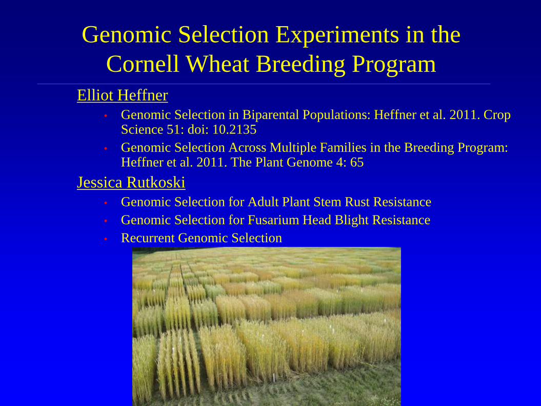
Elliot Heffner

• Genomic Selection in Biparental Populations: Heffner et al. 2011. Crop Science 51: doi: 10.2135

• Genomic Selection Across Multiple Families in the Breeding Program: Heffner et al. 2011. The Plant Genome 4: 65

Jessica Rutkoski

• Genomic Selection for Adult Plant Stem Rust Resistance

• Genomic Selection for Fusarium Head Blight Resistance

• Recurrent Genomic Selection

Genomic Selection Experiments in the

Cornell Wheat Breeding Program

• Biparental Populations

• Cayuga x Caledonia (Soft White Winter)

• 209 DH lines; 399 DArT Markers

• Preharvest Sprouting 16 environments (6 years)

• 9 Milling and Baking Quality traits - 3 years, one location per year

• Foster x KanQueen (Soft Red Winter)

• 175 DH lines; 574 DArT Markers

• 9 Milling and Baking Quality traits - 3 years, one location per year

• Across Multiple Families - Master Nursery

• 400 advanced breeding lines (F7+)

• Augmented field design

• Three locations over 3 years, 2007-2009

• DArT markers ~ 1500 polymorphisms

• 13 agronomic traits

Genomic Selection Experiments in the

Cornell Wheat Breeding Program Elliot Heffner

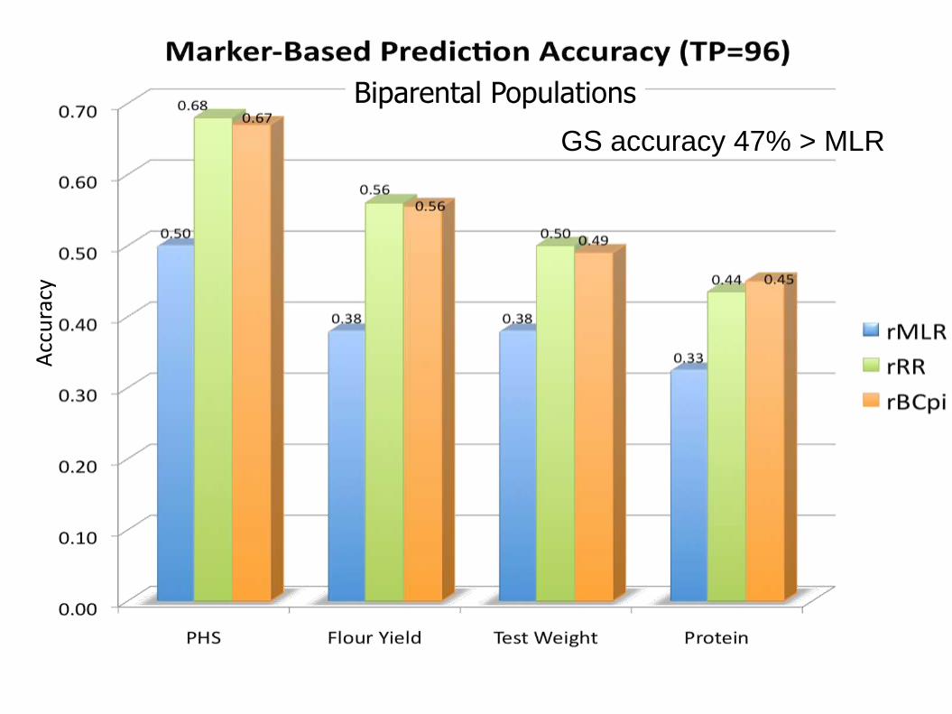
Evaluation Methods for GS in Biparental Populations

• Prediction Models

• MLR: Multiple Linear Regression - Forward/Backward p<0.2

• RR: Ridge Regression BLUP - equal variance, all markers

• BayesCpi: Equal variance, optimized pi for non-zero markers

• Phenotypic Prediction Accuracy

• Based on the Correlation of Phenotypes from TP year with the VP Phenotypes in the Validation Years

• Cross Validation

• Model Training based on one year, validation on remaining (different) years

• Lines in Validation Population (VP) are not included in the Training Population (TP)

• Training Population Sizes = 24, 48, 96

• Marker Number = 64, 128, 256, 384, 399, 574

0.00

0.10

0.20

0.30

0.40

0.50

0.60

0.70

0.80

0.90

PHS Flour Yield Test Weight Protein

0.61

0.50

0.45 0.45

0.84

0.73

0.58 0.60

0.82

0.72

0.57

0.62

Mar

ker

PA /

Ph

en

o P

A

Relative Marker-Based Prediction Accuracy TP=96

MLR

RR

Bcpi

Phenotypic PA 0.82 0.73 0.85 0.84 Phenotypic PA

Biparental Populations

Acc

ura

cy

Biparental Populations

GS accuracy 47% > MLR

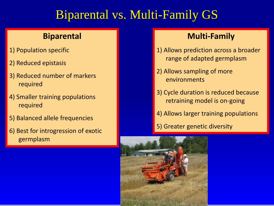
Biparental vs. Multi-Family GS

Multi-Family

1) Allows prediction across a broader range of adapted germplasm

2) Allows sampling of more environments

3) Cycle duration is reduced because retraining model is on-going

4) Allows larger training populations

5) Greater genetic diversity

Biparental

1) Population specific

2) Reduced epistasis

3) Reduced number of markers required

4) Smaller training populations required

5) Balanced allele frequencies

6) Best for introgression of exotic germplasm

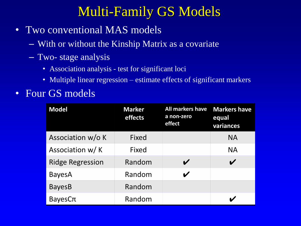
• Two conventional MAS models

– With or without the Kinship Matrix as a covariate

– Two- stage analysis

• Association analysis - test for significant loci

• Multiple linear regression – estimate effects of significant markers

• Four GS models

Model Marker effects

All markers have a non-zero effect

Markers have equal variances

Association w/o K Fixed NA

Association w/ K Fixed NA

Ridge Regression Random ✔ ✔

BayesA Random ✔

BayesB Random

BayesCπ Random ✔

Multi-Family GS Models

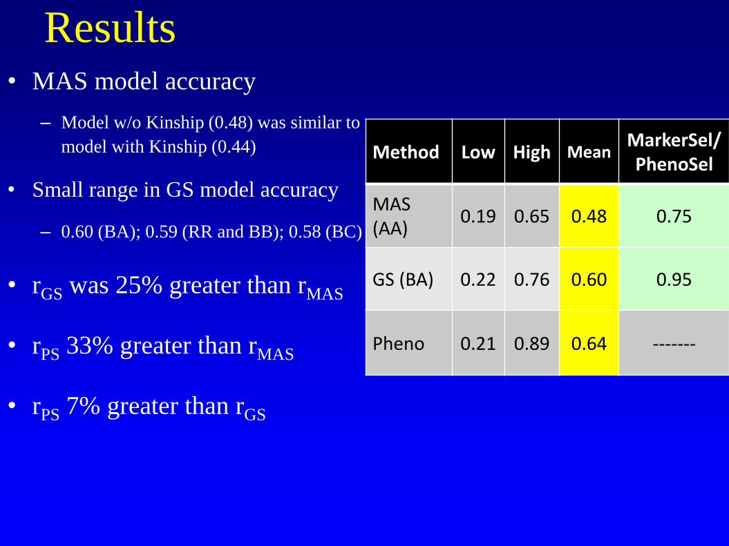
Results • MAS model accuracy

– Model w/o Kinship (0.48) was similar to

model with Kinship (0.44)

• Small range in GS model accuracy

– 0.60 (BA); 0.59 (RR and BB); 0.58 (BC)

• rGS was 25% greater than rMAS

• rPS 33% greater than rMAS

• rPS 7% greater than rGS

Method Low High Mean MarkerSel/PhenoSel

MAS (AA)

0.19 0.65 0.48 0.75

GS (BA) 0.22 0.76 0.60 0.95

Pheno 0.21 0.89 0.64 -------

0.84 0.88

0.92 0.92 0.96

1.01 1.08 1.09

0.00

0.20

0.40

0.60

0.80

1.00

1.20

r GS

/ r P

S Relative GS and PS Prediction Accuracy: Multi-Family

TP Size = 288 Marker Number =1158

NS

0.75/0.89 0.75/0.85 0.76/0.83 0.45/0.49 0.59/0.61 0.57/0.57 0.28/0.26 0.22/0.21

NS

H E A D

D A T E

H E I G H T

P R O T E I N

T E S T

W E I G H T

L O D G I N G

Y I E L D

F L O U R

Y I E L D

P R E

H R V

S P T

*

GS A

ccura

cy/P

S A

ccura

cy

GS/PS

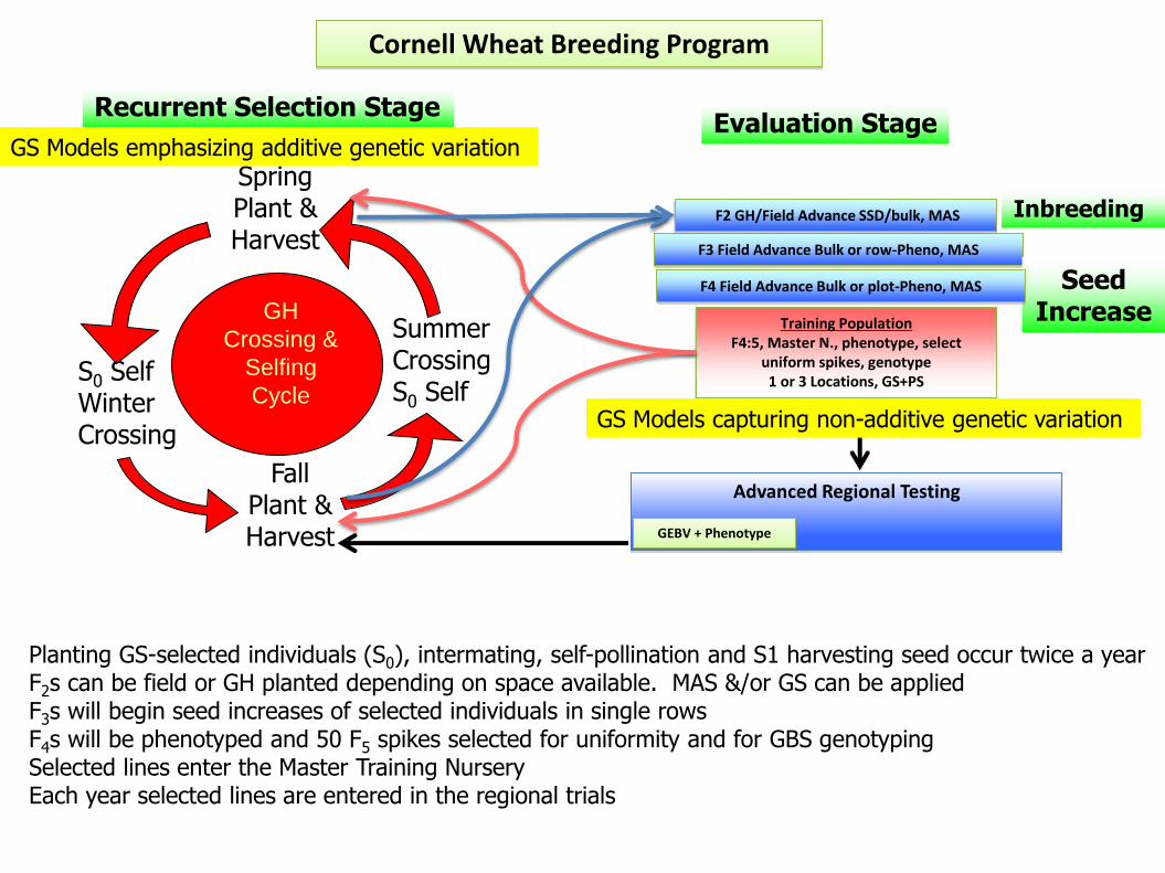
Advanced Regional Testing

F3 Field Advance Bulk or row-Pheno, MAS

Cornell Wheat Breeding Program

GEBV + Phenotype

Training Population F4:5, Master N., phenotype, select

uniform spikes, genotype 1 or 3 Locations, GS+PS

GH

Crossing &

Selfing

Cycle S0 Self Winter Crossing

Spring Plant & Harvest

Fall Plant & Harvest

Summer Crossing S0 Self

Recurrent Selection Stage

F2 GH/Field Advance SSD/bulk, MAS Inbreeding

Seed Increase

Planting GS-selected individuals (S0), intermating, self-pollination and S1 harvesting seed occur twice a year F2s can be field or GH planted depending on space available. MAS &/or GS can be applied F3s will begin seed increases of selected individuals in single rows F4s will be phenotyped and 50 F5 spikes selected for uniformity and for GBS genotyping Selected lines enter the Master Training Nursery Each year selected lines are entered in the regional trials

Evaluation Stage

F4 Field Advance Bulk or plot-Pheno, MAS

GS Models emphasizing additive genetic variation

GS Models capturing non-additive genetic variation

Genomic selection for quantitative disease resistance in wheat

Jessica Rutkoski

Stem rust of wheat, Puccinia graminis f.sp. tritici

Fusarium head blight of wheat Fusarium spp.

• Cooperative Nursery Data – 3 years, 3 nurseries, 60

environments

• Traits: Incidence (Inc), Severity (Sev), Fusarium damaged

kernels (FDK), Incidence/Severity/Kernel quality index (ISK),

Deoxynevalenol (DON), Heading Date (HD)

J. Miller

M. McMullen

M. McMullen

• GS Models: Ridge Regression, Bayesian LASSO, Reproducing

Kernel Hilbert Spaces, Random Forest, Association mapping

with a Q+K matrix+multiple linear regression with markers as

fixed effects

• Population Size: Training – 132, Predicted – 33

• Cross validation: 5 fold, repeated 10 times

Evaluation of GS Models for Fusarium Head

Blight Resistance (Rutkoski et al The Plant Genome In press)

Model Accuracies for Fusarium Head Blight Resistance

0

0.1

0.2

0.3

0.4

0.5

0.6

0.7

HD FDK DON Inc Sev

RF

RKHS

RR

BL

MLRAcc

ura

cy

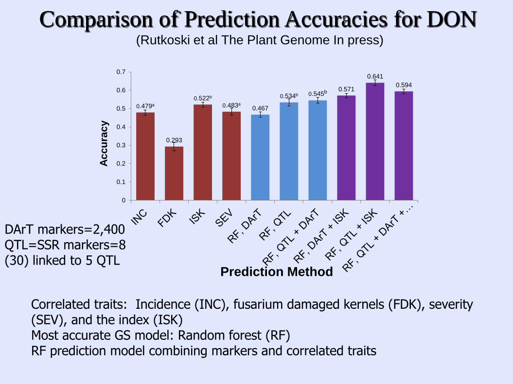
0.479a

0.293

0.522b

0.483a 0.467

0.534b 0.545b 0.571

0.641

0.594

0

0.1

0.2

0.3

0.4

0.5

0.6

0.7

Accu

rac

y

Prediction Method

Comparison of Prediction Accuracies for DON (Rutkoski et al The Plant Genome In press)

Correlated traits: Incidence (INC), fusarium damaged kernels (FDK), severity (SEV), and the index (ISK) Most accurate GS model: Random forest (RF) RF prediction model combining markers and correlated traits

DArT markers=2,400 QTL=SSR markers=8 (30) linked to 5 QTL

Durable Rust Resistance in Wheat

Funded by the Bill & Melinda Gates Foundation

Since the 1999 discovery of virulence on Sr31 in Uganda, Ug99 races have

overcome Sr36 and Sr24 and spread north to Iran and south to South Africa

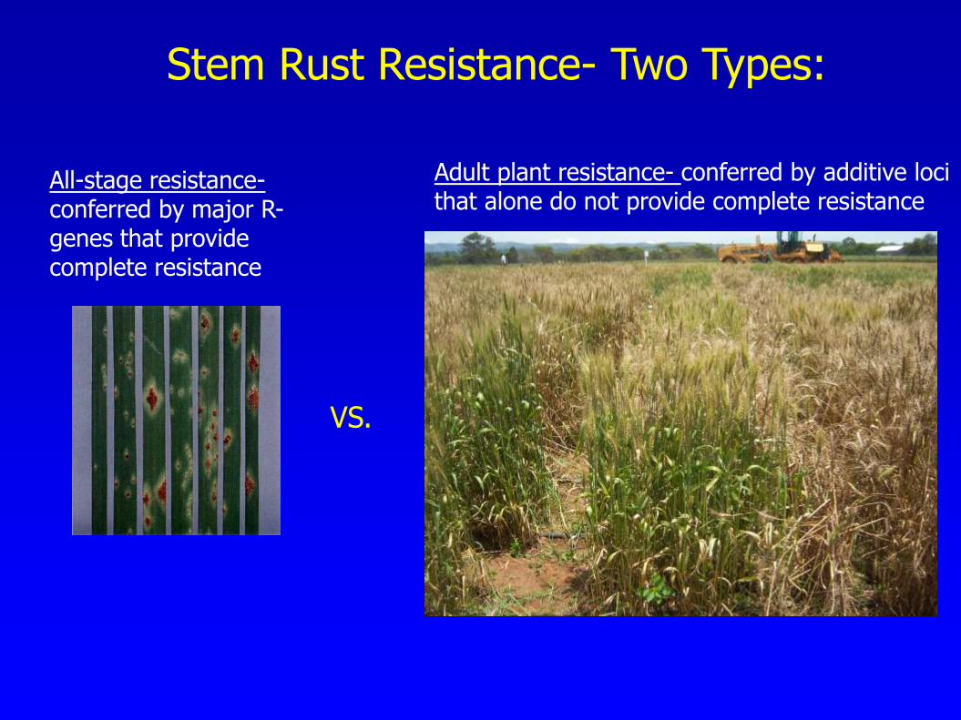
VS.

All-stage resistance- conferred by major R- genes that provide complete resistance

Adult plant resistance- conferred by additive loci that alone do not provide complete resistance

Stem Rust Resistance- Two Types:

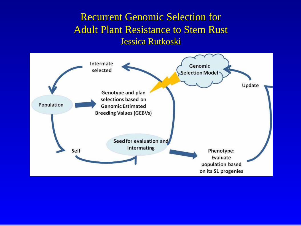
Recurrent Genomic Selection for

Adult Plant Resistance to Stem Rust Jessica Rutkoski

Summary: Genomic Selection

• GS differs from MAS and Association Breeding in that the underlying

genetic control and biological function is not known.

• Breeders can implement GS without the upfront cost of obtaining that

knowledge.

• GS preserves the creative nature of phenotypic selection to sometimes

arrive at solutions outside the engineer’s scope.

• Most important advantages are reductions in the length of the selection

cycle and associated phenotyping cost resulting in greater genetic gain

per year.

Acknowledgements • Special Thanks to Pioneer Hi-Bred for Supporting these Symposia & Graduate Training

• Bill & Melinda Gates Foundation grant to Cornell University for Borlaug Global Rust Initiative

Durable Rust Resistance in Wheat.

• Bill & Melinda Gates Foundation grant to Cornell University & CIMMYT to implement a pilot project

on genomic selection in wheat & maize breeding programs

• USDA Cooperative State Research, Education and Extension Service, Coordinated Agricultural Project

2005-05130-Wheat Applied Genomics

• USDA National Institute of Food and Agriculture, NRI Triticeae Coordinated Agricultural Project

2011-68002-30029 Improving Barley and Wheat Germplasm for Changing Environments

• USDA National Needs Fellowship Grant 2005-38420-15785: Provided Fellowship for Elliot Heffner

• USDA National Needs Fellowship Grant 2008-38420-04755: Provided Fellowship for Jessica

Rutkoski

• Limagrain Europe (France) provided support for Nicolas Heslot

• US Wheat & Barley Scab Initiative: Provided funding for the fusarium head blight research

Questions?