
Assignment Problems with Complementaritiesnguye161/one-sided.pdf · Assignment Problems with...
49
Assignment Problems with Complementarities * Th` anh Nguyen † , Ahmad Peivandi ‡ , Rakesh Vohra § November 2015 Abstract The problem of allocating bundles of indivisible objects without transfers arises in many practical settings, including the assignment of courses to students, of siblings to schools, and of truckloads of food to food banks. In these settings, the complementarities in preferences are small compared with the size of the market. We exploit this to design mechanisms satisfying efficiency, envy-freeness, and asymptotic strategy-proofness. We introduce two mechanisms, one for cardinal and the other for ordinal preferences. When agents do not want bundles of size larger than k, these mechanisms over-allocate each good by at most k - 1 units, ex-post. These results are based on a generalization of the Birkhoff-von Neuman theorem on how probability shares of bundles can be expressed as lotteries over approximately feasible allocations, which is of independent interest. 1 Introduction This paper studies the problem of allocating bundles of indivisible objects without transfers. The problem arises naturally when there are complementarities in preferences—for example, in the assignment of courses to students (Budish [2011]); of CPU time, memory and disk space to computing tasks (Gutman and Nisan [2012]); of truck loads of food to food banks (Houlihan [2006]); of siblings to schools (Abdulkadiro˘ glu et al. [2006]); and of couples to hospital residency positions (Kojima et al. [2013], Ashlagi et al. [2014]). Well-known methods for allocating indivisible goods studied in the literature, such as the prob- abilistic serial mechanism (PS) of Bogomolnaia and Moulin [2001], the competitive equilibrium with equal income mechanism (CEEI) of Hylland and Zeckhauser [1979], and random serial dicta- * This paper is a merger of Peivandi [2012] and Nguyen and Vohra [2013]. † Purdue University, [email protected] ‡ Georgia State University, [email protected] § University of Pennsylvania, [email protected] 1
Transcript of Assignment Problems with Complementaritiesnguye161/one-sided.pdf · Assignment Problems with...

Assignment Problems with Complementarities∗
Thanh Nguyen†, Ahmad Peivandi‡, Rakesh Vohra§
November 2015
Abstract
The problem of allocating bundles of indivisible objects without transfers arises in many
practical settings, including the assignment of courses to students, of siblings to schools, and
of truckloads of food to food banks. In these settings, the complementarities in preferences are
small compared with the size of the market. We exploit this to design mechanisms satisfying
efficiency, envy-freeness, and asymptotic strategy-proofness. We introduce two mechanisms,
one for cardinal and the other for ordinal preferences. When agents do not want bundles of size
larger than k, these mechanisms over-allocate each good by at most k−1 units, ex-post. These
results are based on a generalization of the Birkhoff-von Neuman theorem on how probability
shares of bundles can be expressed as lotteries over approximately feasible allocations, which
is of independent interest.
1 Introduction
This paper studies the problem of allocating bundles of indivisible objects without transfers.
The problem arises naturally when there are complementarities in preferences—for example, in
the assignment of courses to students (Budish [2011]); of CPU time, memory and disk space to
computing tasks (Gutman and Nisan [2012]); of truck loads of food to food banks (Houlihan
[2006]); of siblings to schools (Abdulkadiroglu et al. [2006]); and of couples to hospital residency
positions (Kojima et al. [2013], Ashlagi et al. [2014]).
Well-known methods for allocating indivisible goods studied in the literature, such as the prob-
abilistic serial mechanism (PS) of Bogomolnaia and Moulin [2001], the competitive equilibrium
with equal income mechanism (CEEI) of Hylland and Zeckhauser [1979], and random serial dicta-
∗This paper is a merger of Peivandi [2012] and Nguyen and Vohra [2013].†Purdue University, [email protected]‡Georgia State University, [email protected]§University of Pennsylvania, [email protected]
1

torship (RSD), were designed for unit demand agents. Existing generalizations of these methods
to the multi-unit demand setting fail to preserve the attractive features of their antecedents.1
This paper considers multi-unit demand preferences and proposes an alternative approach to
design mechanisms for both cardinal and ordinal preferences. Our mechanisms exhibit strong
efficiency and equity properties and are asymptotically strategy-proof. However, this come at the
cost of feasibility. These mechanisms are approximately infeasible, equivalently, approximately
wasteful (some resources are withheld from consumption). The degree of infeasibility (or wasteful-
ness) is determined by the degree of complementarity exhibited in the preferences. The smaller the
degree of complementarity in preferences, the smaller the degree of infeasibility (or wastefulness)
in the resulting allocations.
Our first mechanism, called MAXCU,2 works with cardinal utilities. We assume agents are
interested in bundles of, at most, size k, a number significantly smaller than the available supply
of any good. Course allocation is a representative application of this setting. Each good is a
course, and the available supply of each good is the number of seats in the classroom in which the
course will be held. Typically, a student is not able to take more than 5 courses in any term, so
k = 5. MAXCU is ex-ante envy-free, asymptotically strategy-proof, efficient, and approximately
feasible. We show that ex-post, MAXCU might over allocate, at most k − 1 units of each good.
This means, ex-post, we over-allocate at most 4 seats per class. In a classroom with 50 seats, this
can easily be accommodated by adding 4 seats. Alternatively, before running the mechanism, one
could reduce the available number of seats in each class by 4. The resulting ex-post allocations
would be feasible.
Unlike the generalizations of the CEEI due to Budish [2011], which uses ordinal preferences
and is based on computing a competitive equilibrium with equal income, our mechanism is based
on a linear programming approach that maximizes social welfare. In the absence of transfers, a
welfare-maximizing mechanism lacks a device to discourage agents from claiming an excessively
large utility for their most preferred bundle of objects. To see this, consider an example with two
agents, two diamonds, and two rocks. Each agent can consume at most two items and prefers
diamonds to rocks. Any mechanism that implements the unconstrained welfare-optimal solution
1These generalizations are discussed in Section 5.2MAXCU stands for maximizing cardinal utilities.
2

encourages each agent to report a utility of zero for rocks and the largest possible utility for
diamonds. We circumvent this difficulty by imposing ex-ante envy-freeness. This forces an equal
division of diamonds and rocks between the two agents, negating the incentive to exaggerate
utilities.
However, when agents have multi-unit demands, the envy-free welfare-optimal solution might
be fractional and not implementable as a lottery. Second, the solution of the welfare-maximizing
problem may be sensitive to the reported valuations of the agents. To overcome the first difficulty,
we derive a generalization of the Birkhoff-von Neuman theorem about approximate implementa-
tion of fractional solutions. This generalization is of independent interest and can be used as a
component of other mechanisms. This is illustrated in our paper by generalizing the PS mecha-
nism to a setting where agents have multi-unit demands. To overcome the second difficulty, we
perturb the reported utilities before computing the envy-free welfare-optimal solution. With these
ideas, we show that MAXCU is near welfare-maximizing and asymptotically strategy-proof.3
The chief virtue of this method is that it allows the designer to specify the outcome in terms of
probability shares in bundles. Specifically, it gives one greater control over the outcomes.4 Second,
it allows for a succinct description of the mechanism (recall that the set of possible outcomes is
significantly larger than the number of possible bundles that an agent can receive). Subject to a
restriction on preferences, the method has a complexity that is polynomial in the |N | and |G|.
Our second mechanism, called bundled probabilistic serial (BPS), is a natural extension of the
PS mechanism of Bogomolnaia and Moulin [2001]. Here, agents select the best available bundle
and “eat” that bundle at the same rate until one of the items in the bundle is no longer available.
We again use our implementation result to convert the solution into a near feasible lottery. Similar
to Bogomolnaia and Moulin [2001], we show this mechanism to be weakly strategy-proof, envy-
free, and approximately Pareto optimal. Unlike earlier extensions of the PS mechanism to multi-
unit settings that rule out complementarities altogether (as in Che and Kojima [2010] and Kojima
[2009]), our mechanism accommodates limited complementarities in preferences.
The next section introduces notation, the setting and precise restrictions on preferences we
3The relation between envy-freeness and strategy-proofness has been observed, for example, in Jackson andKremer [2007].
4For example, we show how to use this mechanism to implement a competitive equilibrium with equal incomes.
3

impose, and the approximate implementation result. Section 3 introduces and analyzes our first
mechanism. Section 4 describes the second mechanism, which is the generalization of probabilistic
serial mechanism. Section 5 discusses related literature. Section 6 concludes, and the appendix
contains technical proofs.
2 Notation and Approximate Implementation
As noted earlier, the equivalence between probability shares and lotteries relies on the Birkhoff-
von Neuman theorem. This section introduces an approximate generalization of the Birkhoff-von
Neuman theorem that accommodates complementarities in preferences.
In the combinatorial assignment problem, we have a set N of agents and a set G of goods.
For each j ∈ G, the available supply of good j is an integer sj . A bundle is represented by a
non-negative vector B ∈ N|G|, where the jth-coordinate Bj indicates the number of copies of good
j in the bundle B. The size of a bundle B, denoted size(B), is defined as the total number of
items in B, i.e.,∑
j∈GBj . Agent i is interested in obtaining at most one bundle. Here we will
assume that the maximum size of a single bundle is at most k. In the course allocation problem,
for example, students are agents, and each good j corresponds to a course, with the number of
available seats being sj . Each student requires at most 1 seat in each class. In practice, students
can only consume a bundle of size at most 5, so k = 5. In the problem of assigning couples to
hospital residency positions, k = 2. Each bundle consists of 2 positions in the same hospital or in
two different but nearby hospitals.
We assume that each agent receives at most one bundle of goods. To describe the set of
feasible allocations of objects to agents, we introduce the variables xi(B) ∈ 0, 1 for each agent
i and a bundle B such that xi(B) = 1 if agent i obtains bundle B and xi(B) = 0 otherwise.
The set of feasible integral allocations5 can be described by the following constraints. First,
each agent is only interested in bundles of size at most k; thus, we assign xi(B) = 0 for all B of
5We use the term “integral allocation” to distinguish it from an allocation produced by a lottery.
4

size larger than k:
xi(B) ∈ 0, 1 ∀i, B
xi(B) = 0 if size(B) > k
(Integral)
Second, each agent receives at most one bundle of goods:
∑B
xi(B) ≤ 1 ∀i ∈ N. (Demand)
Third, for each type of good j, we do not allocate more than its available supply:
∑i∈N
∑B3j
Bj · xi(B) ≤ sj ∀j ∈ G. (Supply)
We call x a feasible fractional allocation if it satisfies (Demand) and (Supply) and
0 ≤ xi(B) ≤ 1 ∀i, B
xi(B) = 0 if size(B) > k.
(Fractional)
Every lottery over feasible integral allocations corresponds to a feasible fractional allocation
by setting xi(B) equal to the probability that agent i obtains bundle B. The opposite, however,
is not always true, except when k = 1 (this is the Birkhoff-von Neuman theorem).
When k > 1, the Birkhoff-von Neuman theorem fails. Our main result in this section shows
that for general k, every feasible fractional allocation can be expressed as a lottery over integral
allocations that might over-allocate at most k − 1 units of each good. Specifically, to define
approximate supply constraints:
∑i∈N
∑B3j
Bj · xi(B) ≤ sj + k − 1 ∀j ∈ G. (Supply+k-1 )
Our result is the following:
Theorem 2.1 Any (fractional) solution of (Fractional–Demand–Supply) can be implemented as
a lottery over (integral) allocations that satisfy (Integral–Demand–Supply+k-1).
5

The proof of Theorem 2.1 is given in Appendix A. Note that in Theorem 2.1 the over-allocation
amount is independent of market size and only depends on the size of the largest bundles.
To obtain an intuition for this result, consider the case k = 1, which yields the Birkhoff-von
Neuman theorem. Specifically, when k = 1, any (fractional) solution x of (Fractional–Demand–
Supply) can be implemented as a lottery over allocations that satisfy (Integral–Demand–Supply).
To prove a generalization of this theorem, it is useful to view the Birkhoff-von Neuman theorem
in a different but equivalent way. Namely, given any (fractional) x satisfying (Fractional–Demand–
Supply) and any cost vector u, there is an (integral) x satisfying (Integral–Demand–Supply) such
that u · x ≥ u · x. (See Figure 1 for an illustration.)
u
x
x
Figure 1: x can be expressed as a lottery over integral allocations
The statement above no longer holds for k > 1. However, it can be used to generalize the
Birkhoff-von Neuman theorem by allowing x to satisfy a relaxed supply constraint. In particular,
consider the following example.
Example 1 Consider an economy consisting of one copy each of three goods, a, b, c, and 3 agents,
1, 2, 3. Consider a fractional allocation x1(a, b) = x2(b, c) = x3(a, c) = 12 . It is straight-
forward to check that x satisfies both (Demand) and (Supply), but it cannot be implemented as a
lottery over feasible integral allocations. This is because there exists a cost vector u such that for all
feasible integral allocation x, u · x < u · x. Specifically, let u1(a, b) = u2(b, c) = u3(a, c) = 1
and ui(B) = 0 otherwise. We have u · x = 32 . However, because all three goods are in unit
supply, we can allocate at most one of the bundles a, b, b, c or a, c to the agents. That is,
u · x ≤ 1 < 32 = u · x for all integral allocation x.
On the other hand, if we allow over-allocating a good by at most 1 item, then the allocation
6
that assigns a, b to 1 and b, c to 2 will have a cost of 2, which is larger than u · x = 3/2. In
fact, the fractional allocation x can be implemented by the following lottery: with 1/2 probability
assign a, b to 1 and b, c to 2, with 1/2 probability assign a, c to 3.
Our extension of the Birkhoff-von Neuman theorem relies on the following lemma.
Lemma 2.2 Given any (not necessarily non-negative) utility vector ui(B) and any fractional
vector x satisfying Fractional, (Demand), and (Supply), we can find in polynomial time an integral
vector x satisfying (Integral), (Demand), and (Supply+k-1) such that u · x ≥ u · x.
The proof of Lemma 2.2 is provided in Appendix A.1.6
The main idea in the proof of Lemma 2.2 is to take an extreme point solution, x∗, of
(Fractional), (Demand), and (Supply) that maximizes u · x and round it into an integer solution
x. Now x will satisfy (Integral) and (Demand) but violate (Supply), but not by too much. This
last claim follows from the fact that each component of x∗ can appear in at most k inequalities of
the form (Supply) and that x∗ is an extreme point. Hence, no row of (Supply) can contain many
non-zero components of x∗. Thus, in rounding up these components, we limit the magnitude of
the violation of the corresponding constraint.
Given Lemma 2.2, the proof of Theorem 2.1 is as follows.
Proof of Theorem 2.1: For ease of exposition, let Q be the set consisting of all real vectors sat-
isfying (Fractional), (Demand), and (Supply); let Ek be the set of integral solutions to (Integral),
(Demand), and (Supply+k-1).
Suppose Theorem 2.1 does not hold. Then, there is an x ∈ Q that is not in the convex hull of
Ek. Hence, there exists a hyperplane that separates x from Ek. Let u be the vector of coefficients
of that hyperplane. We can choose it so that ux > uz for all z ∈ Ek, which contradicts Lemma 2.2.
The proof of Theorem 2.1 can be converted into an an algorithm to implement x as a lot-
tery over integral solutions of Ek in polynomial time using standard arguments in optimization
(see Grotschel et al. [1981]). However, this algorithm can be impractical for large markets. In
6It is an extension of a recent result in Combinatorial Optimization by Kiraly et al. [2012]. In Kiraly et al.[2012], it is assumed that Bj is either 0 or 1, but our proof does not require such an assumption.
7

Appendix A.2, we provide a practical polynomial time algorithm to construct a lottery with an
expectation that is arbitrarily close to the given vector x in Q. Note that the ε error, in this im-
plementation can be chosen arbitrarily small, independent of the problem parameters. However,
ε influences the running time of the algorithm that constructs the lottery. A smaller ε implies a
longer running time.
3 Maximizing Social Welfare
In this section, we introduce a general mechanism (called MAXCU, which stands for Maximizing
Cardinal Utility) for allocating bundles of objects when agents have cardinal preferences over
bundles. As discussed in the introduction, in the absence of transfers, identifying an integer
allocation in (Demand-Supply) that maximizes a weighted sum of utilities subject to fairness and
incentive compatibility is difficult. The absence of a numeraire, like money, makes it difficult to
discourage agents from claiming an excessively large utility for their most preferred bundle of
objects. To overcome this, we introduce (interim) envy-freeness as a constraint into the program
(Demand-Supply). We then show how Theorem 2.1 can be used to find an approximately feasible
allocation so as to maximize a weighted sum of utilities. Using this result, we show that when
the economy is large, MAXCU is almost efficient and asymptotically strategy-proof.
k-demand Preferences
We first formally define k-demand preferences. If u(B) is an agent’s utility for the bundle B ∈ N|G|,
we require u(∅) = 0 and that u(·) have one of the following properties. The first is that no agent
has preferences for bundles that are too large; that is,
u(B) = 0 ∀B such that size(B) ≥ k + 1. (1)
The second is the monotone cover of the first that allows for free disposal and ensures monotonicity;
that is,
u(B) = maxA⊆B:
u(A) : size(A) ≤ k for B ∈ N|G|. (2)
8

One setting where (1) or (2) will hold is course assignment. Each good j ∈ G is a course, sj is
the number of seats in the course, and each i ∈ N is a student. There is an upper limit, k, on
the number of courses any student can take. k is usually small relative to sj for each j ∈ G. For
example, k will be at most 4, while sj is usually at least 20 and is frequently much larger.
Our mechanism is based on three ideas. First, find a fractional allocation that is envy-free and
maximizes a weighted sum of utilities. Second, approximately implement the fractional allocation
as a lottery. Third, perturb each agent’s utility slightly before finding the optimal fractional
allocation to ensure asymptotic strategy-proofness.
In Section 3.1 we formally introduce the mechanism, MAXCU, and the main result. Section 3.2
establishes the approximate efficicency of MAXCU. Section 3.3 discusses how to approximately
implement the competitive equilibrium outcome as a special case of MAXCU. In Section 3.4, we
prove that by perturbing the objective function in MAXCU, the mechanism is asymptotically
strategy-proof.
3.1 Mechanism MAXCU
To implement MAXCU, choose a positive weight wi for each agent i and solve the linear program
of maximizing∑
i∈N∑
B wi ·ui(B)xi(B) subject to (Demand-Supply) and the envy-free condition
defined below.
An allocation x satisfying (Demand-Supply) is envy-free if
∑B
ui(B)xi(B) ≥∑B
ui(B)xj(B) ∀i ∀j 6= i. (EnvyFree)
In words, agent i prefers the lottery he or she is faced with to the lottery offered to any other
agent. Moulin [1995] (page 166) lists envy-freeness as one of “the two most important tests of
equity.”.
Formally, the mechanism MAXCU is defined as follows.
Definition 3.1 Given positive weights w, let x∗ be an optimal solution of
max∑i∈N
∑B
wi · ui(B)xi(B) : s.t. (Demand), (Supply), (EnvyFree). (3)
9

(If there are multiple solutions, select one with a fixed tie-breaking rule. Note, xi(B) = 0 for all i
and B is a feasible solution to 3.)
By Theorem 2.1, x∗ can be implemented as a lottery over integral assignments satisfying
(Demand) and (Supply+k-1). The mechanism MAXCU takes as input a report of each agent’s
utility function, returns the optimal (fractional) solution to program (3), and implements it as a
lottery.
To illustrate this mechanism, consider the following example.
Example 2 Consider an economy consisting of three goods, a, b, c, each with unit supply, and 3
agents, 1, 2, 3. Each agent can consume at most 2 items. Each agent’s utility for a single item
is $1. Agent 1’s utility for a, b is $4; agent 2’s utility for b, c is $4, and agent 3’s utility for
a, c is $4. All other bundles of size 2 give utility of $2 to each agent.
Take the weight vector w to be the vector of all 1s. Then, MAXCU will find a fractional
allocation x∗ that maximizes total utility subject to (Demand), (Supply), and (EnvyFree). This
gives x∗1(a, b) = x∗2(b, c) = x∗3(a, c) = 1/2. As in Example 1, x∗ can be implemented as a lottery
over near-feasible allocations as follows: with 1/2 probability assign a, b to 1 and b, c to 2 with
1/2 probability assign a, c to 3.
Mechanism MAXCU has several attractive properties. First, it gives the designer control over
the outcome through selection of the weights wi. For example, by choosing wi = 1 for all i,
mechanism MAXCU selects an allocation of maximum total utility. We show in Section 3.2 that
this mechanism is almost optimal among the envy-free randomized mechanisms. For another
choice of the wis, mechanism MAXCU can implement a generalization of the CEEI mechanism
of Hylland and Zeckhauser [1979]. This is discussed in Section 3.3.
Second, mechanism MAXCU is incentive compatible in large markets. Specifically, in Sec-
tion 3.4 we show that if (3) has a unique optimal solution, one can implement x∗ in a way that is
asymptotically strategy-proof.7 Thus, under this condition, mechanism MAXCU is approximately
efficient subject to ex-ante envy-free and is asymptotically strategy-proof.
7The assumption that (3) has a unique optimal solution is a mild one, because we can always guarantee this byperturbing wi slightly.
10
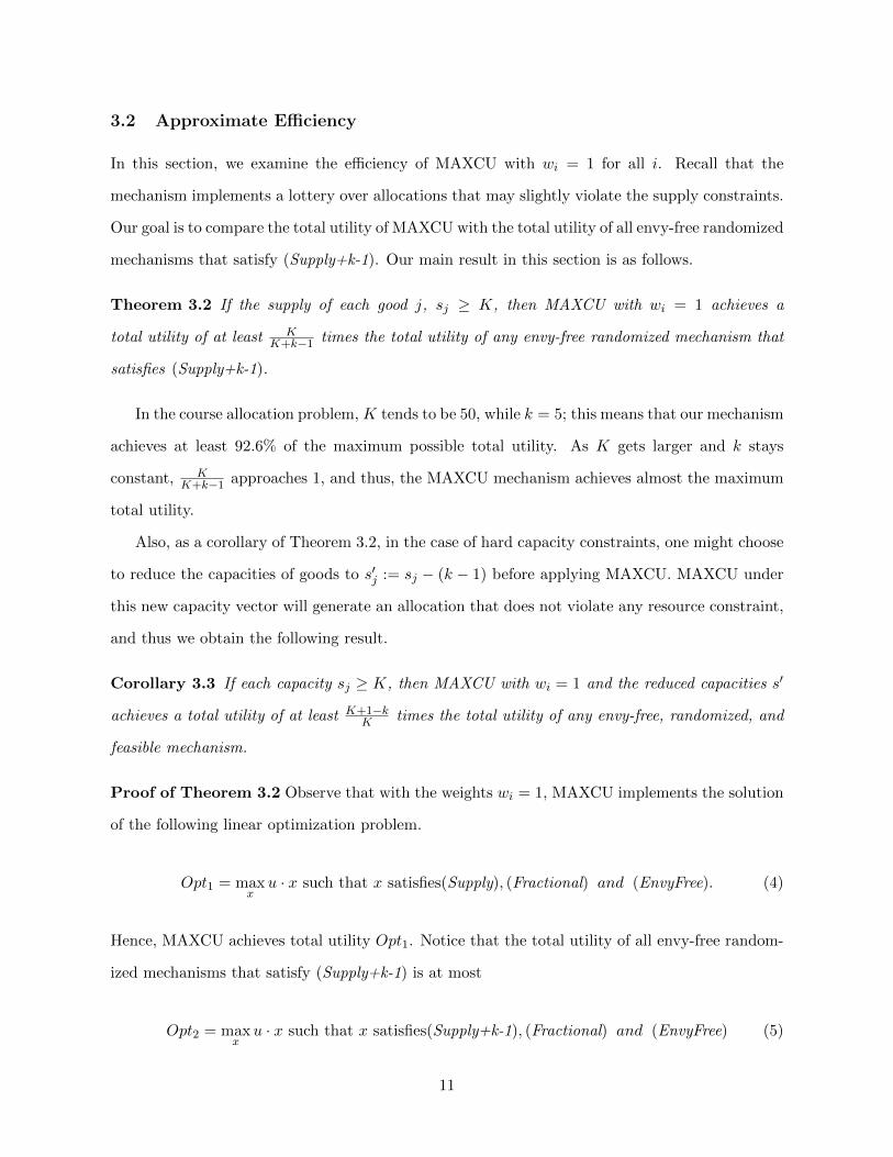
3.2 Approximate Efficiency
In this section, we examine the efficiency of MAXCU with wi = 1 for all i. Recall that the
mechanism implements a lottery over allocations that may slightly violate the supply constraints.
Our goal is to compare the total utility of MAXCU with the total utility of all envy-free randomized
mechanisms that satisfy (Supply+k-1). Our main result in this section is as follows.
Theorem 3.2 If the supply of each good j, sj ≥ K, then MAXCU with wi = 1 achieves a
total utility of at least KK+k−1 times the total utility of any envy-free randomized mechanism that
satisfies (Supply+k-1).
In the course allocation problem, K tends to be 50, while k = 5; this means that our mechanism
achieves at least 92.6% of the maximum possible total utility. As K gets larger and k stays
constant, KK+k−1 approaches 1, and thus, the MAXCU mechanism achieves almost the maximum
total utility.
Also, as a corollary of Theorem 3.2, in the case of hard capacity constraints, one might choose
to reduce the capacities of goods to s′j := sj − (k − 1) before applying MAXCU. MAXCU under
this new capacity vector will generate an allocation that does not violate any resource constraint,
and thus we obtain the following result.
Corollary 3.3 If each capacity sj ≥ K, then MAXCU with wi = 1 and the reduced capacities s′
achieves a total utility of at least K+1−kK times the total utility of any envy-free, randomized, and
feasible mechanism.
Proof of Theorem 3.2 Observe that with the weights wi = 1, MAXCU implements the solution
of the following linear optimization problem.
Opt1 = maxx
u · x such that x satisfies(Supply), (Fractional) and (EnvyFree). (4)
Hence, MAXCU achieves total utility Opt1. Notice that the total utility of all envy-free random-
ized mechanisms that satisfy (Supply+k-1) is at most
Opt2 = maxx
u · x such that x satisfies(Supply+k-1), (Fractional) and (EnvyFree) (5)
11

Thus, to prove our theorem, it is enough to show that:
Opt1 ≥K
K + k − 1Opt2. (6)
To see (6), let x∗ be the optimal solution of (5). Thus, x∗ satisfies (Supply+k-1), (Fractional), and
(EnvyFree). Consider KK+k−1x
∗. It is straightforward to verify that KK+k−1x
∗ continues to satisfy
(Fractional) and (EnvyFree). Furthermore, because sj ≥ K:
sjsj + k − 1
≥ K
K + k − 1.
Therefore, KK+k−1(sj + k− 1) ≤ sj . This shows that if we scale x∗ down by a factor of K
K+k−1 , the
new solution, KK+k−1x
∗, satisfies (Supply). Recall that Opt1 is the maximum total utility for all
allocations satisfying (Supply), (Fractional), and (EnvyFree). Hence,
K
K + k − 1x∗ · u ≤ Opt1.
This implies Opt1 ≥ KK+k−1Opt2.
3.3 Implementing the CEEI mechanism with MAXCU
In the original CEEI mechanism, agents are restricted to unit demands and are endowed with
equal budgets of fictitious money. Each agent i has a utility uij for good j. We extend each
agent’s utility function to probability shares in each good in the obvious way:
ui(x) =∑j
uijxij ,
where xij is the probability share or fraction of good j allocated to agent i. A competitive
equilibrium allocation of probability shares in the economy just described is determined. Under
the unit demand restriction, the Birkhoff-von Neuman theorem implies that the competitive
equilibrium allocation can be implemented as a lottery. From the properties of a competitive
equilibrium, it follows that the CEEI mechanism is ex-ante Pareto optimal and ex-ante envy-
12

free. Recall that there exist positive weights wii∈N (Negishi weights) such that this competitive
equilibrium allocation maximizes weighted social welfare subject to ex-ante envy-freeness. Hence,
MAXCU with the correct Negishi weights can implement the CEEI mechanism.
The idea extends to the case of k-demand preferences as well. Namely, we extend each agent’s
utility function over bundles to a utility function over bundles of divisible goods. This extension is
concave. Treating the goods as divisible, we give each agent the same fictitious budget. Market-
clearing prices (one price for each good rather than each bundle) exist (see Appendix B.1 for
a short proof via the celebrated results of Arrow-Debreu-McKenzie). This fractional allocation,
while feasible, may not be implementable. Under Theorem 2.1 it can be implemented so that it
over-allocates each good by at most k−1 units.8 This is a generalization of the CEEI mechanism,
which we call the bundled competitive equilibrium from equal income B-CEEI mechanism.
Notice that an equilibrium allocation of bundles can always be obtained by maximizing a
suitable weighted sum of utilities subject to (Demand), (Supply); furthermore, an outcome of a
competitive equilibrium with equal budgets is envy-free. Thus, our mechanism MAXCU with the
proper weights wi can implement the outcome of the B-CEEI mechanism.
We continue Example 2 to illustrate how one can use MAXCU with a suitable weight vector
w to implement the B-CEEI mechanism.
Example 3 Consider Example 2, provide each agent with $1. In Appendix B.1, we show that
there exists item prices of individual goods a, b, and c such that market clears. In this example,
pa = pb = pc = 1. With a budget of $1, to maximize his or her utility, agent 1 would purchase
1/2 of the bundle a, b; similarly, agent 2 would purchase 1/2 of the bundle b, c and agent 3
would purchase 1/2 of the bundle a, c. This gives us the fractional allocation x∗.
From the property of a competitive equilibrium with equal budgets, we know that x∗ satisfies
(EnvyFree), (Demand), and (Supply); furthermore, x∗ is Pareto optimal. Thus, x∗ can be obtained
as an optimal solution of
max∑i∈N
∑B
wi · ui(B)xi(B) : s.t. (Demand), (Supply), (EnvyFree),
8Equivalently, we find prices at which the excess demand for each good is at most k − 1.
13

for a proper positive weight vector w. In fact, as in Example 2, choosing wi = 1 will suffice to
select x∗. x∗, then, is implemented as a lottery over near-feasible allocations, with 1/2 probability
assigns a, b to 1 and b, c to 2; and with 1/2 probability assigns a, c to 3.
It is instructive to compare the B-CEEI mechanism to Budish’s (Budish [2011]) generalization
of the CEEI mechanism—call it the A-CEEI mechanism. A-CEEI is a randomized mechanism for
the combinatorial assignment problem based on computing an approximate competitive equilib-
rium from approximately equal incomes. B-CEEI is a randomized mechanism for the combinatorial
assignment problem based on computing an exact competitive equilibrium from equal incomes.
The preference information required of agents by A-CEEI is ordinal but of B-CEEI is cardinal.
A-CEEI and B-CEEI are both approximately Pareto optimal, asymptotically strategy-proof, and
violate the resource constraints. Budish bounds the violation in terms of the Euclidean distance
between the supply vector and the vector of the number of goods allocated. That bound is√
min2k,|G||G|2 . In B-CEEI, the maximum violation in each type of good is at most k − 1. The
two bounds are not comparable. A-CEEI is ex-post approximately envy-free while B-CEEI is
ex-ante envy-free. The notion of approximate envy-free used in Budish [2011] can be described
in the following way. Suppose agent i is awarded the bundle B and agent i′ awarded the bundle
B′. If agent i prefers B′ to B, then, there is a j ∈ B′ such that agent i prefers B to B′ \ j. When
complementarities in preferences are strong, this is a weak requirement. To see why, suppose
agent i assigns positive utility to bundle B′ but zero utility to any strict subset of B′.
In the next subsection, we introduce notation to define precisely what is meant by asymptotic
strategy-proofness as well as prove that the mechanism just described is asymptotically strategy-
proof.
3.4 Asymptotic Strategy-Proofness
In this section, we define the notion of asymptotic strategy-proofness when agents have cardinal
utilities. First, we specify how the economy will “grow”. In this we follow Che and Kojima [2010].
For each q ∈ N, denote the set of objects in the q−economy by G and the set of agents by Nq.
Each object j ∈ G in the q−economy has sqj ≥ k copies. Furthermore, limq→∞ sqj = ∞ for all
j ∈ G. The preference of each agent in N q is determined by the agent’s type. Let Θ be a finite
14

set of types, and for each θ ∈ Θ, let nqθ be the number of agents of type θ in the q−economy.
The type of an agent encodes his or her preferences, which are represented by a von-Neumann
Morgenstern utility function defined on bundles of goods. For an agent of type θ ∈ Θ, let
uθ(B) ≥ 0 be his utility for bundle B ∈ Nq|G|. We will also use the notation uθi (B) (or for short
ui(B) ) for the utility of agent i for bundle B when his type is θ. We assume that an agent’s
utility depends exclusively on his type and outcome. Furthermore, we assume for each type, the
utility function satisfies either (1) or (2). Without loss of generality, we also assume uθ(∅) = 0 for
all types θ. Given a lottery (a probability distribution) over a set of bundles, an agent’s utility
is his expected utility from the lottery.
We assume that the number of copies of each object and the number of agents of each type
grow at the same rate as q.
Assumption 3.1 There exist positive real numbers (s∗j )j∈G and (n∗θ)θ∈Θ such that: limq→∞sqjq =
s∗j and limq→∞|nqθ|q = n∗θ ∈ R, ∀θ ∈ Θ.
Given a type profile, an allocation is envy-free if all agents weakly prefer the lottery assigned
to them to any lottery assigned to another. That is,
uθi(xi) ≥ uθi(xj).
Let A denote the set of (approximately) feasible allocations. For every |N q| > 0, a mechanism
Φ(Nq) is a mapping from a profile of agents’ types to a lottery over (approximately) feasible
allocations. More precisely,
Φ(Nq) : Θ|Nq | → ∆(A).
We sometimes use Φ instead of Φ(Nq) for short.
It will be useful to consider a mechanism from the perspective of an agent i. Let
Φ|Nq |i : Θ×Θ|N
q−1| → ∆(Ai),
where Ai denotes the possible bundles that agent i obtains, and Φi(θi, θ−i) denotes the lottery
over bundles that agent i receives when he or she reports θi and other agents report θ−i.
15
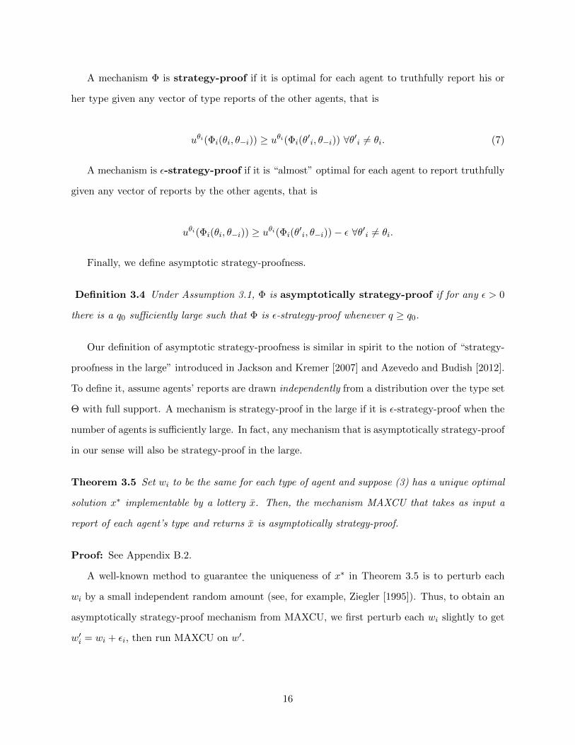
A mechanism Φ is strategy-proof if it is optimal for each agent to truthfully report his or
her type given any vector of type reports of the other agents, that is
uθi(Φi(θi, θ−i)) ≥ uθi(Φi(θ′i, θ−i)) ∀θ′i 6= θi. (7)
A mechanism is ε-strategy-proof if it is “almost” optimal for each agent to report truthfully
given any vector of reports by the other agents, that is
uθi(Φi(θi, θ−i)) ≥ uθi(Φi(θ′i, θ−i))− ε ∀θ′i 6= θi.
Finally, we define asymptotic strategy-proofness.
Definition 3.4 Under Assumption 3.1, Φ is asymptotically strategy-proof if for any ε > 0
there is a q0 sufficiently large such that Φ is ε-strategy-proof whenever q ≥ q0.
Our definition of asymptotic strategy-proofness is similar in spirit to the notion of “strategy-
proofness in the large” introduced in Jackson and Kremer [2007] and Azevedo and Budish [2012].
To define it, assume agents’ reports are drawn independently from a distribution over the type set
Θ with full support. A mechanism is strategy-proof in the large if it is ε-strategy-proof when the
number of agents is sufficiently large. In fact, any mechanism that is asymptotically strategy-proof
in our sense will also be strategy-proof in the large.
Theorem 3.5 Set wi to be the same for each type of agent and suppose (3) has a unique optimal
solution x∗ implementable by a lottery x. Then, the mechanism MAXCU that takes as input a
report of each agent’s type and returns x is asymptotically strategy-proof.
Proof: See Appendix B.2.
A well-known method to guarantee the uniqueness of x∗ in Theorem 3.5 is to perturb each
wi by a small independent random amount (see, for example, Ziegler [1995]). Thus, to obtain an
asymptotically strategy-proof mechanism from MAXCU, we first perturb each wi slightly to get
w′i = wi + εi, then run MAXCU on w′.
16

4 Generalizing the Probabilistic Serial Mechanism
Mechanism MAXCU requires that agents communicate cardinal preferences, which is sometimes
impractical. Hence, we turn our attention to mechanisms that rely on ordinal information alone.
We generalize the well-known probabilistic serial (PS) mechanism for allocating indivisible goods
when agents have strict preferences and unit demands (introduced by Bogomolnaia and Moulin
[2001]). The PS mechanism begins with each agent consuming, at the same constant rate, his or
her most preferred object. When the supply of an object is exhausted, agents consuming that
object switch to consuming the next available object on their preference list. At termination, the
fraction of each object an agent has consumed determines the probability shares in that object.
These probability shares can be implemented as a lottery over feasible allocations. It is well
known that the PS mechanism is envy-free, ordinally efficient, and asymptotically strategy-proof.
We define ordinal efficiency for cases when agents have preferences over bundles rather than
single objects. Recall that a bundle is represented by a non-negative vector B ∈ N|G|, where the
jthcoordinate indicates the number of copies of good j in the bundle B. A bundle can also be
represented as a multi-set, and in some of the examples below it will be convenient to do so.
Assume that agents have strict preferences over bundles. Let ≺i be agent i’s ordinal preference
ranking over bundles. As each agent receives a lottery over allocations, we extend a preference or-
dering over bundles to a partial ordering over lotteries of bundles via stochastic dominance. Recall
that a lottery over allocations induces probability shares x over bundles that satisfy (Demand)
and (Supply). Thus, we may identify each lottery with a solution of (Demand) and (Supply).9 An
allocation x satisfying (Demand) and (Supply) weakly stochastically dominates an allocation y for
agent i, if for all B ⊆ G: ∑SiB
xi(S) ≥∑SiB
yi(S).
Allocation x stochastically dominates y for agent i, if the above inequality holds strictly for some
bundle B. A mechanism is ordinally efficient if there is no other random assignment that weakly
stochastically dominates the mechanism’s allocation with respect to all agents’ preferences over
bundles.
9Recall, each feasible fractional solution of (Demand) and (Supply) does not correspond to a lottery over feasibleintegral allocations.
17
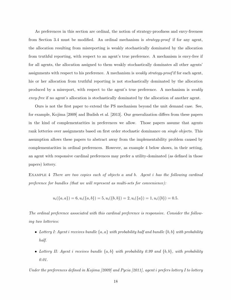
As preferences in this section are ordinal, the notion of strategy-proofness and envy-freeness
from Section 3.4 must be modified. An ordinal mechanism is strategy-proof if for any agent,
the allocation resulting from misreporting is weakly stochastically dominated by the allocation
from truthful reporting, with respect to an agent’s true preference. A mechanism is envy-free if
for all agents, the allocation assigned to them weakly stochastically dominates all other agents’
assignments with respect to his preference. A mechanism is weakly strategy-proof if for each agent,
his or her allocation from truthful reporting is not stochastically dominated by the allocation
produced by a misreport, with respect to the agent’s true preference. A mechanism is weakly
envy-free if no agent’s allocation is stochastically dominated by the allocation of another agent.
Ours is not the first paper to extend the PS mechanism beyond the unit demand case. See,
for example, Kojima [2009] and Budish et al. [2013]. Our generalization differs from these papers
in the kind of complementarities in preferences we allow. Those papers assume that agents
rank lotteries over assignments based on first order stochastic dominance on single objects. This
assumption allows these papers to abstract away from the implementability problem caused by
complementarities in ordinal preferences. However, as example 4 below shows, in their setting,
an agent with responsive cardinal preferences may prefer a utility-dominated (as defined in those
papers) lottery.
Example 4 There are two copies each of objects a and b. Agent i has the following cardinal
preference for bundles (that we will represent as multi-sets for convenience):
ui(a, a) = 6, ui(a, b) = 5, ui(b, b) = 2, ui(a) = 1, ui(b) = 0.5.
The ordinal preference associated with this cardinal preference is responsive. Consider the follow-
ing two lotteries:
• Lottery I: Agent i receives bundle a, a with probability half and bundle b, b with probability
half.
• Lottery II: Agent i receives bundle a, b with probability 0.99 and b, b, with probability
0.01.
Under the preferences defined in Kojima [2009] and Pycia [2011], agent i prefers lottery I to lottery
18

II, since under lottery I agent i has a higher chance of receiving copies of object a. However, agent
i has a higher expected utility for lottery II.
4.1 Bundled Probabilistic Serial Mechanism
A natural generalization of the PS mechanism for multi-unit demand is to have agents consume
bundles rather than individual objects. When the supply of an object is exhausted, agents switch
to their most preferred bundle not containing objects whose supply has been exhausted. This
mechanism, which we call the Bundled Probabilistic Serial (BPS) mechanism, returns probability
shares in bundles. Therefore, it produces outcomes that, in general, cannot be implemented. Re-
call that Kojima [2009] and Budish et al. [2013] circumvent this difficulty by assuming preferences
satisfy first order stochastic dominance on single objects. In this restricted case, the BPS mech-
anism reduces to the PS mechanism. However, if we assume preferences satisfy the k-demand
condition, we may invoke Theorem 2.1. Under these conditions, the BPS mechanism is envy-free,
ordinally efficient, strategy-proof, and over-allocates each good by at most k − 1 units. These
results, along with a formal description of the BPS mechanism, are stated below.
To define the BPS mechanism formally, let t(0) = 0 ≤ t(1) ≤ t(2) ≤ t(v) ≤ t(v + 1)... be the
instances in time when the supply of at least one good falls to zero. Also, let BPS(v) be the
fractional allocation that the algorithm produces up to time t(v). Initially BPS(0) = 0, which
is an allocation in which no agent receives an object. At time t(v), the set of goods in non-zero-
supply is denoted G(v). Initially, G(0) = G. Let zv be the integral allocation, not necessarily
feasible, where each agent is assigned his or her most preferred bundle consisting only of objects
in G(v). Let mj(v) be the total number of copies of object j that appear in zv.10 Denote by rvj
the measure of object j consumed at time t(v), therefore r0j = 0. The BPS mechanism consists of
the following steps:
• Starting with available supply of G(v − 1), the latest time at which the current supply of
good j would be exhausted is
tj(v) = supt ∈ [0, 1]|rv−1j +mj(v − 1)(t− t(v − 1)) ≤ sj.
10Agents are allowed to consume multiple copies of an object in G(v).
19

• Therefore, the first instance at which any good is exhausted is t(v) = minj∈G(v−1) tj(v).
• At time t(v), the set of goods with non-zero supply is
G(v) = G(v − 1) \ j ∈ G(v − 1)|tj(v) = t(v).
• The measure of object j consumed up to time t(v) is
rvj = rv−1i +mj(v − 1)(tj(v)− tj(v − 1)).
• The allocation returned by the BPS mechanism at time t(v) is
BPS(v) = BPS(v − 1) + (t(v)− t(v − 1))zv−1.
The term (t(v) − t(v − 1)) represents the fraction of the bundle in zv−1 that each agent
receives in the time interval (t(v − 1), t(v)].
• BPS terminates at time t(v) where v is the smallest index such that t(v) = 1.
Theorem 4.1 The BPS mechanism is ordinally efficient, envy-free, weakly strategy-proof, and
under k-demand preferences can be implemented so that it over-allocates each good by at most
k − 1 units.
As the first three items admit a proof similar to the proof of Theorem 1 and Proposition 1
in Bogomolnaia and Moulin [2001], we content ourselves with a sketch. (See Appendix C for a
formal proof.)
The greedy nature of BPS implies that a fractional assignment that stochastically dominates
the BPS assignment must be infeasible. Similarly, for weak strategy-proofness, if a misreport
stochastically dominates truth telling, the feasibility constraints would be violated. Envy-freeness
follows from the fact that once BPS stops allocating probability shares of a bundle to agents,
then at least one of the objects in that bundle is unavailable. Therefore, no other agent can be
allocated probability shares from that bundle afterwards.
20
The last item follows from Theorem 2.1 as the probability shares produced by BPS satisfy
(Demand) and (Supply).
4.2 Limited Complementarities
We extend BPS to environments in which agents are interested in larger bundles with limited
complementarities. We assume complementarities are present only in bundles with size at most
k. This extension is analogous to the extensions of unit-demand preferences considered in Kojima
[2009], Pycia [2011], and Budish et al. [2013].
In particular, we define limited complementary preferences (LCP) as follows. There is an
underlying partition P1, P2 . . . , Pt of G such that |Pr| ≤ k for all r = 1, . . . , t. We assume this
partition is common knowledge. Furthermore, we assume agents are interested in at most one
copy of each good. The preferences of agents have complementarities among the goods inside
each Pr, but not across different elements of the partition. Namely, each agent i has preferences,
i, on the following set of bundles
B = B : ∃r s.t B ⊂ Pr.
As an example, suppose four goods 1, 2, 3, 4. The given partition is (1,2); (3,4). Preferences of
an agent, for example, can be (1, 2) (2) (3, 4) (1) (3) (4) ∅.
Based on this linear preference order, we can define preferences over expected assignments
that possibly assign a positive probability over large bundles. Specifically, given an expected
assignment x, let xi(B) =∑
S:S∩Pt=B xi(S). Thus, x is an expected assignment that assigns
positive probability to subsets of the elements of the partition and B ⊂ Pt. As an example,
assume x assigns 1/2 probability to the bundle (1,2,3) and probability 1/2 to the bundle (1,2),
then, under the partition (1,2); (3,4), x assigns probability 1 to (1,2) and probability 1/2 to (3).
Next, we define preferences over expected assignments. Namely, agent i prefers x to y if he prefers
x to y, where the preference between x and y is given by the stochastic dominance relation.
LCP contains the preferences defined in Kojima [2009], Pycia [2011], and Budish et al. [2013]
as a special case. It suffices to choose as the underlying partition one that places each object into
its own set.
21
LCP preferences arise in the bandwidth allocation problem. Blocks within the same spectrum
band are complements up to a certain maximum number of blocks, and blocks from different
bands are substitutes (see Schweitzer [2014]). Another example is consumption over time. Each
element of the partition represents the set of available objects in a time period. Within a time
period, there is no restriction on preferences; however, objects from different time periods are
substitutes.
Preferences with both complementarities and substitutes have have been studied before; see
Sun and Yang [2006] and Teytelboym [2014]. Their set-up is different in that goods in the same
element are substitutes while they are complements across elements.
The extension of PS is straightforward. Each agent, at the speed of 1, is allocated probability
shares of his or her most preferred available bundle consisting of objects from of a single element
of the partition. There are two constraints in this mechanism. First, the total time an agent
spends consuming subsets of an element of a partition is 1. Second, the mechanism stops when
there is no available bundle in which an agent is interested. We call this extended mechanism
the bundled probabilistic serial mechanism under limited complementarity assumption(BPSLC).
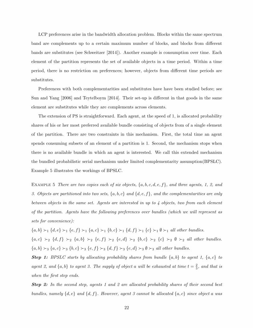
Example 5 illustrates the workings of BPSLC.
Example 5 There are two copies each of six objects, a, b, c, d, e, f, and three agents, 1, 2, and
3. Objects are partitioned into two sets, a, b, c and d, e, f, and the complementarities are only
between objects in the same set. Agents are interested in up to 4 objects, two from each element
of the partition. Agents have the following preferences over bundles (which we will represent as
sets for convenience):
a, b 1 d, e 1 e, f 1 a, c 1 b, c 1 d, f 1 c 1 ∅ 1 all other bundles.
a, c 2 d, f 2 a, b 2 e, f 2 e, d 2 b, c 2 c 2 ∅ 2 all other bundles.
a, b 3 a, c 3 b, c 3 e, f 3 d, f 3 e, d 3 ∅ 3 all other bundles.
Step 1: BPSLC starts by allocating probability shares from bundle a, b to agent 1, a, c to
agent 2, and a, b to agent 3. The supply of object a will be exhausted at time t = 23 , and that is
when the first step ends.
Step 2: In the second step, agents 1 and 2 are allocated probability shares of their second best
bundles, namely d, e and d, f. However, agent 3 cannot be allocated a, c since object a was
22

exhausted in step 1. Therefore, agent 3 is allocated probability shares in b, c. Note that all three
agents are allocated bundles from a, b, c for 23 unit of time, and this mechanism allocates bundles
from a partition to agents for at most one unit of time. Therefore, in this step, probability shares
are allocated for 13 period of time, and this step terminates at time 2
3 + 13 .
Step 3: The mechanism continues to allocate probability shares from d, e and d, f to agents
1 and 2. However, the mechanism starts allocating agent 3 probability shares from e, f. After
23 period of time the supply of object d is exhausted. Therefore, this step of the mechanism stops
at time 23 + 1
3 + 23 .
Step 4: Note that agents 1 and 2 will not be allocated probability shares from e, f, since both
were allocated probability shares of bundles from the partition d, e, f for one period of time. In
this step, agents 1 and 2 are allocated probability shares from b, c, and agent 3 is allocated a
probability share from e, f. This step ends after 16 unit of time, when the supply of object b is
exhausted.
Step 5: The mechanism continues to allocate probability shares from bundle e, f to agent 3.
Agents 1 and 2 receive probability shares from c. The mechanism stops after 16 unit of time,
since the supply of both objects e and f are exhausted.
The mechanism terminates as all agents have received probability shares of bundles from each
partition for 1 unit of time. The mechanism returns the following probability shares: Agent 1
receives a, b with probability 23 , d, e with probability 1, b, c with probability 1
6 , and c with
probability 16 . Agent 2 receives a, c with probability 2
3 , d, f with probability 1, b, c with
probability 16 , and c with probability 1
6 . Agent 3 is allocated a, b with probability 23 , b, c with
probability 13 , and e, f with probability 1.
Similar to the BPS mechanism in Section 4.1, the expected assignment may not be imple-
mentable. However, it is approximately implementable as given in the following result.
23
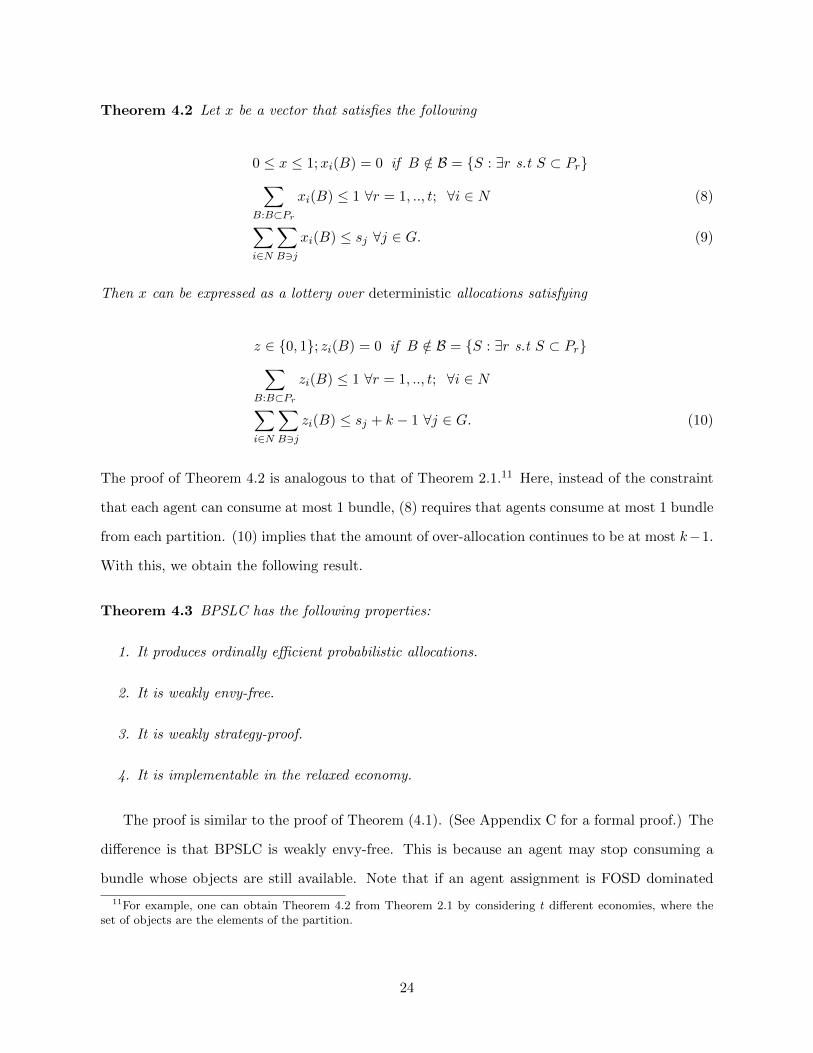
Theorem 4.2 Let x be a vector that satisfies the following
0 ≤ x ≤ 1;xi(B) = 0 if B /∈ B = S : ∃r s.t S ⊂ Pr∑B:B⊂Pr
xi(B) ≤ 1 ∀r = 1, .., t; ∀i ∈ N (8)
∑i∈N
∑B3j
xi(B) ≤ sj ∀j ∈ G. (9)
Then x can be expressed as a lottery over deterministic allocations satisfying
z ∈ 0, 1; zi(B) = 0 if B /∈ B = S : ∃r s.t S ⊂ Pr∑B:B⊂Pr
zi(B) ≤ 1 ∀r = 1, .., t; ∀i ∈ N
∑i∈N
∑B3j
zi(B) ≤ sj + k − 1 ∀j ∈ G. (10)
The proof of Theorem 4.2 is analogous to that of Theorem 2.1.11 Here, instead of the constraint
that each agent can consume at most 1 bundle, (8) requires that agents consume at most 1 bundle
from each partition. (10) implies that the amount of over-allocation continues to be at most k−1.
With this, we obtain the following result.
Theorem 4.3 BPSLC has the following properties:
1. It produces ordinally efficient probabilistic allocations.
2. It is weakly envy-free.
3. It is weakly strategy-proof.
4. It is implementable in the relaxed economy.
The proof is similar to the proof of Theorem (4.1). (See Appendix C for a formal proof.) The
difference is that BPSLC is weakly envy-free. This is because an agent may stop consuming a
bundle whose objects are still available. Note that if an agent assignment is FOSD dominated
11For example, one can obtain Theorem 4.2 from Theorem 2.1 by considering t different economies, where theset of objects are the elements of the partition.
24

by the assignment of another agent, then because of the symmetry of this mechanism and the
feasibility constraints, one of the feasibility constraints would be violated.
The BPS mechanism under the k-demand preference assumption is suitable for environments
where agents are interested in only a few objects. If k is large, the BPS mechanism may allocate
to agents bundles that are too large, resulting in large ex-post envy. This problem is also present
in the RSD mechanism. Example 6 below shows why BPSLC is fairer compared to RSD and
BPS.
Example 6 Suppose there are 2 agents and 4 objects, numbered 1, 2, 3, 4. Objects are parti-
tioned into two subsets, 1, 2 and 3, 4. Agent 1 ranks objects as 1, 2, 3, 4, but agent 2 ranks
objects as 3, 4, 1, 2.
RSD as well as BPS will allocate one agent his best bundle, 1, 3, and the other his worst
bundle, 2, 4. However the BPSLC allocates agent 1 the bundle 1, 4, and agent 2 gets 2, 3.
Clearly this is an improvement in terms of fairness.
4.3 Asymptotic properties of BPS
While the BPS mechanism is not strategy-proof, it is, as we show in this section, asymptotically
strategy-proof. The notion of asymptotic strategy-proofness differs from that given in section 3.3.
There we had defined asymptotic strategy-proofness for cardinal preferences; see equation (7) and
definition 3.4. Here we must modify the definition to account for ordinal preferences.
Recall that agent is endowed with a type θ ∈ Θ, and there are a finite number of types. In
this case, a type θ determines an agent’s ranking over bundles.
Definition 4.4 Allocation x ε−stochastically dominates y for agents i with respect to ordinal
preference i if ∑SiB
xi(S) + ε >∑SiB
yi(S).
An ordinal mechanism is asymptotically strategy-proof if for all ε > 0 there is a q sufficiently large
such that the allocation returned from truthful reporting ε−stochastically dominates any allocation
resulting from misreporting in the q−economy.
Theorem 4.5 BPS and BPSLC are asymptotically strategy-proof.
25

Proof: Asymptotic strategy-proofness follows from characterizing the limit of the BPS mecha-
nism, which generalizes Theorem 1 in Che and Kojima [2010]. To prove this, we first define a
continuum economy as the limit of the q—economy as q →∞. Let BPS∗ be the BPS mechanism
in the continuum economy. We show that the BPS mechanisms converge to BPS∗. The difficulty
in our case, compared with Che and Kojima [2010], arises because of the complementarities in
agents’ preferences. In the unit demand case, once consumption of an object begins, it continues
until its supply is exhausted. In our case, consumption of an object occurs in fits and starts.
Therefore, a simple adaptation of their proof is not possible. We show this result by proving
that the available supply of each object at each step of the mechanism converges to the available
supply in the continuum model. For a complete proof, see Appendix D.12
5 Related Literature
The literature on the allocation of indivisible goods is extensive and can be divided into two
strands. The first strand of literature develops and studies mechanisms that specify a lottery
over outcomes, while the second strand focuses on mechanisms that specify probability shares
in objects. Examples of the first type of mechanism are random serial dictatorship (RSD) and
top-trading with random endowments (TTC).13 Neither explicitly randomizes over each possible
outcome given the large number of possible outcomes. Instead, they specify a procedure for
assigning goods to agents from a randomly chosen starting point.14 These methods are typically
strategy-proof and Pareto optimal but lack other desirable properties like ordinal efficiency and
envy-freeness. Indeed, strategy-proofness and ex-post Pareto optimality rule out most mechanisms
except some form of dictatorship (Papai [2001], Ehlers and Klaus [2003] and Hatfield [2009]).
Hashimoto [2013] has proposed a generalization of the RSD mechanism that is feasible and
strategy-proof and converges to the outcomes of a version of the CEEI mechanism (for bundles) in
12In the unit demand case, the PS and RSD mechanisms were shown to be asymptotically equivalent by Che andKojima [2010]. Liu and Pycia [2013] generalized this result to show that any two mechanisms that satisfy ordinalefficiency, symmetry, and asymptotic strategy-proofness coincide asymptotically. PS and RSD are two examplesof mechanisms in this class. Pycia [2011] generalized this result to the case of agents with multi-unit demand,assuming that agents rank lotteries over assignments based on first-order stochastic dominance on single objects.
13See, for example, Abdulkadiroglu and Sonmez [1998] and references therein.14In RSD, for example, agents are randomly assigned a priority ordering that determines who gets to choose first.
In TTC, agents are randomly assigned a good, which they can then trade with others.
26

large markets. To obtain feasibility, Hashimoto’s mechanism withholds some goods. Specifically,
a fraction ε of goods that are in “excess” demand are withheld, but ε goes to 0 while the number
of agents goes to infinity. The rate at which ε converges to 0 is sensitive to the type-space and
the prior distribution. The drawback of this approach is that the economy may be implausibly
large before the proposed allocations are acceptably close to meeting the desired criteria. In our
setting, one can also withhold k − 1 units from each good to ensure feasibility. However, unlike
Hashimoto [2013], our “excess” demand is measured by an additive error and does not depend on
market size or prior distributions.
A drawback of dictatorship mechanisms is that they may perform poorly in terms of ex-ante
efficiency and fairness, especially when agents have multi-unit demands (see, for example, Budish
and Cantillon [2012]). This particular deficiency of dictatorship mechanisms naturally increases
interest in more ex-ante efficient and equitable mechanisms, regardless of their strategy-proofness.
These mechanisms specify probability shares in objects rather than lotteries over feasible out-
comes. Examples are PS and CEEI (Bogomolnaia and Moulin [2001], Hylland and Zeckhauser
[1979]). Under the unit demand assumption, there is an equivalence between probability shares
and lotteries over feasible outcomes. As probability shares are in a sense “easier” to specify, these
mechanisms produce outcomes with many more desirable properties than either RSD or TTC.
Moreover, several recent papers (Kojima and Manea [2010], Azevedo and Budish [2012]) show
that when the economy is large, these mechanisms are essentially strategy-proof.
Generalizations of these mechanisms to multi-unit demand have been proposed (see Kojima
[2009] and Budish [2011]). There are significant differences between these mechanisms and ours,
and these are described in Section 3.3 and Section 4. Our work is also related to Budish et al.
[2013], which considers a bi-hierarchical constraint structure and obtains exact implementation.15
In the context of course allocation, the bi-hierarchical constraint structure severely restricts the
set of bundles that can be allocated to students. Our paper does no more than limit the size of
the bundle students can be assigned. In the context of course allocation and similar settings in
which agents desire bundles of limited size, such a restriction is natural.
Recently, Akbarpour and Nikzad [2014] generalized Budish et al. [2013] to consider feasibility
15In the combinatorial optimization literature, this structure is called an intersecting laminar system.
27

constraints more complex than simple capacity constraints. They do not consider complemen-
tarities in preferences, and their approximation result holds only probabilistically rather than
ex-post. Specifically, they bound the probability that a given good is not over-allocated by a
certain amount, while our result guarantees that ex post all goods are not over-allocated by more
than k − 1.16
Our paper also contributes to the literature on approximate competitive equilibria with indi-
visibilities and non-convex preferences (Starr [1969], Broome [1972], Emmerson [1972], Mas-Colell
[1977], and Garratt [1995]). These approximation results bite only when the size of the economy
as measured by the number of goods becomes very large—usually too large for applications like
the course allocation problem. This is a consequence of the generality of the constraint structure.
Our approach, on the other hand, takes advantage of the “limited” complementarity property in
the preferences to get a stronger bound that is independent of market size.
6 Conclusion
Attractive mechanisms for the allocation of indivisible goods when there are complementarities
in preferences are rare. The positive results known have usually been obtained for continuum
markets. This paper introduces two new mechanisms for allocating indivisible goods that are
approximately feasible. The novel feature of these mechanisms is that the error bounds do not
depend on the size of the market but on the degree of complementarity exhibited by the prefer-
ences.
Acknowledgements
We thank the referees, Eric Budish and Roger Myerson, for their many useful suggestions.
16For example, in the context of course allocation, the bounds in Akbarpour and Nikzad [2014] are too large tobe applicable.
28

References
A. Abdulkadiroglu and T. Sonmez. Random Serial Dictatorship and the Core from Random
Endowments in House Allocation Problems. Econometrica, 66(3):689–702, May 1998.
A. Abdulkadiroglu, P. Pathak, A. E. Roth, and T. Sonmez. Changing the boston school choice
mechanism. Nber working papers, National Bureau of Economic Research, Inc, Jan. 2006.
M. Akbarpour and A. Nikzad. Approximate random allocation mechanisms. Working Paper,
2014.
I. Ashlagi, M. Braverman, and A. Hassidim. Stability in large matching markets with comple-
mentarities. Operations Research, 62(4):713–732, 2014.
E. M. Azevedo and E. Budish. Strategyproofness in the large as a desideratum for market design.
In ACM Conference on Electronic Commerce, page 55, 2012.
A. Bogomolnaia and H. Moulin. A new solution to the random assignment problem. Journal of
Economic Theory, 100(2):295–328, October 2001.
J. Broome. Approximate equilibrium in economies with indivisible commodities. Journal of
Economic Theory, 5(2):224–249, 1972.
E. Budish. The combinatorial assignment problem: Approximate competitive equilibrium from
equal incomes. Journal of Political Economy, 119(6):1061 – 1103, 2011.
E. Budish and E. Cantillon. The multi-unit assignment problem: Theory and evidence from
course allocation at harvard. American Economic Review, 102(5):2237–71, 2012.
E. Budish, Y.-K. Che, F. Kojima, and P. Milgrom. Designing random allocation mechanisms:
Theory and applications. American Economic Review, 103(2):585–623, September 2013.
Y.-K. Che and F. Kojima. Asymptotic Equivalence of Probabilistic Serial and Random Priority
Mechanisms. Econometrica, 78(5):1625–1672, 09 2010.
L. Ehlers and B. Klaus. Coalitional strategy-proof and resource-monotonic solutions for multiple
assignment problems. Social Choice and Welfare, 21(2):265–280, 2003.
29

R. D. Emmerson. Optima and market equilibria with indivisible commodities. Journal of Eco-
nomic Theory, 5(2):177–188, 1972.
R. Garratt. Decentralizing lottery allocations in markets with indivisible commodities. Economic
Theory, 5(2):295–313, 1995.
M. Grotschel, L. Lovasz, and A. Schrijver. The ellipsoid method and its consequences in combi-
natorial optimization. Combinatorica, 1(2):169–197, 1981.
A. Gutman and N. Nisan. Fair allocation without trade. In Proceedings of the 11th International
Conference on Autonomous Agents and Multiagent Systems - Volume 2, AAMAS ’12, pages
719–728, 2012.
T. Hashimoto. The generalized random priority mechanism with budgets. Working Paper, 2013.
J. W. Hatfield. Strategy-proof, efficient, and nonbossy quota allocations. Social Choice and
Welfare, 33(3):505–515, 2009.
P. Houlihan. How food banks came to love the free market. Chicago Booth Magazine, pages
34–39, 2006.
A. Hylland and R. Zeckhauser. The efficient allocation of individuals to positions. Journal of
Political Economy, 87(2):293–314, April 1979.
M. O. Jackson and I. Kremer. Envy-freeness and implementation in large economies. Review of
Economic Design, 11(3):185–198, 2007.
T. Kiraly, L. Lau, and M. Singh. Degree bounded matroids and submodular flows. Combinatorica,
32(6):703–720, 2012. ISSN 0209-9683.
F. Kojima. Random assignment of multiple indivisible objects. Mathematical Social Sciences, 57
(1):134–142, 2009.
F. Kojima and M. Manea. Incentives in the probabilistic serial mechanism. Journal of Economic
Theory, 145(1):106–123, 2010.
30

F. Kojima, P. A. Pathak, and A. E. Roth. Matching with couples: Stability and incentives in
large markets. The Quarterly Journal of Economics, 128(4):1585–1632, 2013.
Q. Liu and M. Pycia. Ordinal efficiency, fairness, and incentives in large markets. Working Paper,
2013.
A. Mas-Colell. Indivisible commodities and general equilibrium theory. Journal of Economic
Theory, 16(2):443–456, 1977.
H. Moulin. Cooperative Microeconomics. London, Prentice Hall, 1995.
T. Nguyen and R. Vohra. The allocation of indivisible objects via rounding. Working Paper,
2013.
S. Papai. Strategyproof and nonbossy multiple assignments. Journal of Public Economic Theory,
3(3):257–271, 2001.
A. Peivandi. Random allocation of bundles. Working paper, Northwestern University, 2012.
M. Pycia. Ordinal efficiency, fairness, and incentives in large multi-unit-demand assignments.
Working Paper, 2011.
S. M. Schweitzer. Large-scale Multi-item Auctions: Evidence from Multimedia-supported Experi-
ments. KIT Scientific Publishing, 2014.
R. M. Starr. Quasi-equilibria in markets with non-convex preferences. Econometrica, 37(1):25–38,
1969.
N. Sun and Z. Yang. Equilibria and indivisibilities: gross substitutes and complements. Econo-
metrica, 74(5):1385–1402, 2006.
A. Teytelboym. Gross substitutes and complements: a simple generalization. Economics Letters,
123(2):135–138, 2014.
G. Ziegler. Lectures on Polytopes. Graduate Texts in Mathematics. Springer New York, 1995.
ISBN 9780387943657.
31

A Appendix A: Iterative Rounding Algorithm
A.1 Proof of Lemma 2.2
The proof uses an algorithm called the Iterative Rounding Algorithm (IRA). The goal of the
(IRA) is to identify an x ∈ arg maxc · x : Dx ≤ d, x ≥ 0 that is integral. Here D is an
arbitrary matrix and d an arbitrary vector. The (IRA) begins by choosing an extreme point
x∗ ∈ arg maxc ·x : Dx ≤ d, x ≥ 0. If x∗ is integral, we are done. If not, the (IRA) will eliminate
one or more constraints and resolve the linear program.
Step 0: Initiate xopt := x∗.
Step 1: If xopt is integral, stop and output xopt; otherwise, continue to either Step 2a or 2b.
Step 2a: If any coordinate of xopt is integral, fix the value of those coordinates, and update the
linear program.
To describe the updated linear program, let C and C be the set of columns of D that
correspond to the non-integer and integer valued coordinates of xopt, respectively. Let DC ,
and DC be the sub-matrix of D that consists of columns in C and the complement C,
respectively. Similarly, for vector x, let xC and xC be the sub-vector of x that consists of
all coordinates in C and C. The updated linear program is:
maxcC · xC : s.t. DC · xC ≤ d−DC · xopt
C.
In other words, we replace c by cC ; x by xC ; D by DC and d by d−DC · xopt
Cand move to
Step 3.
Step 2b If all coordinates of xopt are fractional, delete certain rows of D (to be specified later)
and the corresponding constraints from the linear program. Update the linear program and
move to Step 3.
Step 3 Solve the updated linear program maxc·x s.t. Dx ≤ d to get an extreme point solution.
Let this be the new xopt and return to Step 1.
32
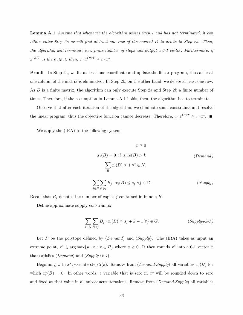
Lemma A.1 Assume that whenever the algorithm passes Step 1 and has not terminated, it can
either enter Step 2a or will find at least one row of the current D to delete in Step 2b. Then,
the algorithm will terminate in a finite number of steps and output a 0-1 vector. Furthermore, if
xOUT is the output, then, c · xOUT ≥ c · x∗.
Proof: In Step 2a, we fix at least one coordinate and update the linear program, thus at least
one column of the matrix is eliminated. In Step 2b, on the other hand, we delete at least one row.
As D is a finite matrix, the algorithm can only execute Step 2a and Step 2b a finite number of
times. Therefore, if the assumption in Lemma A.1 holds, then, the algorithm has to terminate.
Observe that after each iteration of the algorithm, we eliminate some constraints and resolve
the linear program, thus the objective function cannot decrease. Therefore, c · xOUT ≥ c · x∗.
We apply the (IRA) to the following system:
x ≥ 0
xi(B) = 0 if size(B) > k∑B
xi(B) ≤ 1 ∀i ∈ N.
(Demand)
∑i∈N
∑B3j
Bj · xi(B) ≤ sj ∀j ∈ G. (Supply)
Recall that Bj denotes the number of copies j contained in bundle B.
Define approximate supply constraints:
∑i∈N
∑B3j
Bj · xi(B) ≤ sj + k − 1 ∀j ∈ G. (Supply+k-1 )
Let P be the polytope defined by (Demand) and (Supply). The (IRA) takes as input an
extreme point, x∗ ∈ arg maxu · x : x ∈ P where u ≥ 0. It then rounds x∗ into a 0-1 vector x
that satisfies (Demand) and (Supply+k-1).
Beginning with x∗, execute step 2(a). Remove from (Demand-Supply) all variables xi(B) for
which x∗i (B) = 0. In other words, a variable that is zero in x∗ will be rounded down to zero
and fixed at that value in all subsequent iterations. Remove from (Demand-Supply) all variables
33

xi(B) for which x∗i (B) = 1 and adjust the right hand sides of (Supply) accordingly. In other
words, a variable set to 1 (or 0) by x∗ is fixed at 1 (or 0) in all subsequent iterations. In the
system that remains, pick a non-negative extreme point that optimizes the vector u and repeat.
At some iteration, when the remaining supply of good j is s′j , we may obtain an extreme point,
with each variable taking a value strictly less than 1. Call it y. At this point we must execute
step 2(b)—that is, identify a constraint to be omited. We show in Lemma A.2, below that in this
case, there exists a j ∈ G such that
∑i∈N
∑B3j
Bj · dy∗i (B)e ≤ s′j + k − 1.
For each such j, remove the corresponding constraint (Supply) and proceed to Step 3. Suppose
the (IRA) terminates in a 0-1 vector x.
There are three observations to be made about x.
1. At each iteration, inequality (Demand) holds. Thus, x satisfies (Demand).
2. By Lemma A.1, u · x ≥ u · x∗.
3. Because xi(B) = 1 only if x∗i (B) > 0, it follows that for the inequalities in (Demand)
discarded,∑
i∈N Bj ·∑
B3j xi(B) ≤ sj + k − 1.
We now show that the constraints in Step 2(b) to be discarded do indeed exist.
Lemma A.2 Let ui(B) be any utility function. Let S0(i),S1(i) be the set of bundles that xi(B)
for all B ∈ S0(i) have been fixed to be 0, and xi(B) for all B ∈ S1(i) have been fixed to be 1,
respectively.
Let x∗ be an extreme point of the linear program
maxu · x : x satisfies (Demand) and (Supply), xi(B) = 0∀B ∈ S0(i);xi(B) = 1∀B ∈ S1(i).
Assume that x∗i (B) < 1 for all i ∈ N and B such that B /∈ S0(i) ∪ S1(i). (In other words, x∗i (B)
34

has not been fixed). Then, there exists a j ∈ G such that
∑i∈N
∑B:j∈B
Bjdx∗i (B)e ≤ sj + k − 1.
To prove Lemma A.2, assume for a contradiction that 0 < x∗i (B) < 1 for all i, B and∑
i∈N∑
B:j∈B Bjdx∗i (B)e >
sj + k − 1 for all j ∈ G. Because∑
i∈N∑
B:j∈B Bjdx∗i (B)e is an integer, we have
∑i∈N
∑B:j∈S
Bjdx∗i (B)e ≥ sj + k ∀j ∈ G. (11)
We use (11) to contradict the fact that x∗ is an extreme point. Recall that an extreme point
of a linear program has the following property:
The number of non-zero variables in an extreme point x∗ is equal to the number of
linearly independent and binding constraints in (Demand) and (Supply).
The contradiction arises from trying to reconcile two things. First, each column of (Demand)
and (Supply) that correspond to a positive component of x∗ consists of exactly two non-zero entries.
Second, each row corresponding to j ∈ G intersects at least sj + k columns that correspond to
positive components of x∗. By a counting argument, we show that it is impossible to achieve both
without violating the extreme point property of x∗.
Given the extreme point x∗, we credit each non-zero variable x∗i (B) with a single token. We
then redistribute these tokens to the binding, linearly independent constraints in a particular way.
We show that if (11) holds, then each binding constraint will get at least one token with one token
left over. This proves that the number of non-zero variables x∗i (B) is larger than the number of
binding, linearly independent constraints, which is a contradiction.
We redistribute the tokens as follows. Credit x∗i (B) fraction of the tokens to the constraint
corresponding to agent i (Demand). Credit Bj1−x∗i (B)
k to each constraint corresponding to each
good j ∈ B. Notice that this is feasible because the size of each bundle is∑
j∈GBj ≤ k.
35

If the constraint corresponding to agent i binds, then the number of tokens this constraint is
credited with is∑
S xi(B) = 1. For a binding constraint corresponding to good j, we have:
∑i∈N
∑B3j
Bjxi(B) = sj . (12)
The total quantity of tokens that this constraint obtains is
∑B,i∈N :x∗i (B)>0
Bj1− x∗i (B)
k=
1
k
∑B,i∈N :x∗i (B)>0
Bj −1
k
∑i∈N
∑B3j
Bjxi(B).
From (11) and (12) this number of tokens is at least
1
k(sj + k − sj) = 1.
Thus, any binding constraint j (Demand) is credited with at least 1 token.
Hence, we have shown that the amount of tokens given at the beginning (which is the number
of non-zero x∗ variables) has been redistributed to the binding constraints, so that each is credited
with at least 1 token. Thus, the number of non-zero x∗ variables is at least the number of binding
constraints.
Now, the equality obtains only if for every nonzero x∗i (B), the size of bundle B is exactly
k—that is,∑
j∈GBj = k. Furthermore, the constraint corresponding to agent i as well as all the
constraints corresponding to all j ∈ B binds. However, in this case, one can show that the set of
binding constraints is not linearly independent. To see this, consider the sum of all the binding
constraints in Supply: ∑j∈G
∑i,B:B3j
Bjx∗i (B) =
∑j∈G
sj .
Because for each x∗i (B) > 0,∑
j∈B Bj = k, this sum can be rewritten as
k ·∑i,B
x∗i (B) =∑j
sj .
This last expression is the sum of all the constraints in (Demand), contradicting linear indepen-
dence of the binding constraints. By this we have shown that the number of non-zero variables in
36

an extreme point solution is larger than the number of linearly independent binding constraints.
A.2 An Algorithm to Construct a Lottery
Recall that Theorem 2.1 shows that any x ∈ Q can be expressed as a convex combination of
points in Ek. In this section, we show how to (approximately) decompose any x ∈ Q into a
convex combination of points in Ek.
Assume Ek is bounded with diameter D. Denote by |x− y| the Euclidean distance between x
and y. Recall that we have a subroutine that will, for any fractional x ∈ Q and any cost vector
c, return an integral x ∈ Ek such that cx ≥ cx.
Given this subroutine, we exhibit a polynomial time algorithm that, for a given point x ∈ Q,
finds at most d + 1 integral points in Ek, the convex hull of which is arbitrarily close to x. The
algorithm also returns a lottery over these d+ 1 integral vectors, the expectation of which is close
to x.
Given a fractional solution x ∈ Q, let
B(x, δ) = z : satisfying (Demand) and |z − x| ≤ δ.
We assume there exists δ > 0 such that B(x, δ) ⊂ Q. Notice that for our purpose, this
assumption is without loss of generality, because otherwise we can always choose x′ in the interior
of Q close to x.
Given an allowable error ε > 0, the algorithm is the following.
Algorithm In each step, maintain a subset B of points in Ek. Each iteration consists of the
following steps.
1. Compute y ∈ conv(B) that is closest to x. If |y − x| < ε, the algorithm terminates.
2. Otherwise, because y is the closest point to x in B, y lies in a hyperplane of conv(B). Thus,
there exists a subset B′ ⊂ B of size at most d such that y ∈ conv(B′). (Recall d is the
dimension).
37

Consider z = x + δ x−y|x−y| . Notice, z ∈ Q because B(x, δ) ∈ Q. Use the rounding algorithm
to find an integral z′ ∈ Ek, such that
< z, x− y > ≤ < z′, x− y > .
3. Update B := B′ ∪ z′ and repeat.
To show that the algorithm terminates in polynomial time, we show that after each iteration,
the distance |x− y| is reduced by at least a constant factor. To prove this, let y′ be the point in
the interval [z′, y] that is closest to x. We will prove the following.
Figure 2:
Claim A.3 There exists 0 < γ < 1 that depends on D and δ such that |x− y′| < (1− γ)|x− y|
Proof: Let t be the point in the interval (z′, y) such that < t − z, x − y >= 0. Because
< z, x− y >≤< z′, x− y >, such a t exists. See Figure 2.
Now,
|x− y|2
|x− y′|2=|t− y|2
|t− z|2=|t− z|2 + (|x− z|+ |x− y|)2
|t− z|2≥ |t− z|
2 + δ2
|t− z|2
We have |t − z| ≤ |z′ − z|. Furthermore, because the diameter of Ek is D, |z′ − z| ≤ D. Thus,
|t− z| ≤ D.
Hence, we obtain
|x− y|2
|x− y′|2≥ D2 + δ2
D2.
38

Thus, there exists 0 < γ < 1, depending on D and δ such that
|x− y′| < (1− γ)|x− y|,
which is what we need to prove.
The claim above shows that after each iteration, the distance between x and y is reduced by
at least a factor of (1− γ). Consider K = ln(D/ε)γ ; we have
D(1− γ)K ≤ ε.
Thus, after at most K iterations, the algorithm will terminate.
B Equilibrium & Asymptotic Strategy-Proofness
B.1 Equilibrium Existence in B-CEEI
In this section, we show how to use the standard Arrow-Debreu-Mckenzie argument to estab-
lish the existence of market-clearing item prices when agents have non-unit demands. As be-
fore, assume an agent i ∈ N who consumes a fraction xi(B) of bundle B enjoys a utility of∑B ui(B)xi(B), where ui(B) is the utility derived from bundle B. To invoke the Arrow-Debreu-
McKenzie theorem, we need to express agent i’s utility not as a function of bundles but as a
concave function of the quantities of the individual goods consumed. If we give agent i the vector
z ∈ [0, 1]|G|, where zj is interpreted to be a fraction of good j, agent i’s utility can be represented
as
Ui(z) = max∑B
ui(B)xi(B)
s.t.∑B3j
Bj · xi(B) ≤ zj ∀j ∈ G
xi(B) ≥ 0 ∀i ∈ N, ∀ bundle B
Notice, Ui(z) is concave in z.
If agent i has an income of W , the unit price of j ∈ G is pj , and agent i’s consumption problem
39

is
maxUi(z)
s.t.∑j∈G
pjzj ≤W
zj ≥ 0 ∀j ∈ G
Let Di(p) be the set of optimal solutions to the above program. It follows immediately from the
usual arguments that there must exist a price vector p∗ and zi ∈ Di(p∗) for all i ∈ N such that∑
i∈N zij ≤ sj for all j ∈ G.
B.2 Proof of Theorem 3.5
Fix a q sufficiently large. In the sequel, we suppress the dependence on q. Recall that the set of
types, Θ, is finite. Let θi be the type reported by agent i, and denote by nθ the number of agents
reporting type θ. Also let wθi be the weight that the mechanism chooses for an agent of type θi.
Consider the following program for finding a utilitarian allocation that is envy-free:
max∑i∈N
∑B
wθi · uθi(B)xθii (B) (13)
∑B
xθii (B) ≤ 1 ∀i ∈ N (14)
∑i∈N
∑B3j
xθii (B) ≤ sj ∀j ∈ G (15)
∑B
uθi(B)xθii (B) ≥∑B
uθi(B)xθjj (B) ∀i, j (16)
Recall that we can set xθii (B) = 0 whenever size(B) > k. Call (13-16) the disaggregate
formulation.
Introduce variables yθ(B) to denote the “aggregate” amount of bundle B that all agents
reporting θ get. Namely, if we consider an anonymous solution of (13-16), that is xθii (B) =
xθjj (B) whenever θi = θj = θ, then yθ(B) = nθx
θii (B). Now consider the following “aggregate”
40

formulation:
max∑θ∈Θ
∑B
wθ · uθ(B)yθ(B) (17)
∑B
1
nθyθ(B) ≤ 1 ∀θ ∈ Θ (18)
∑t∈Θ
∑B3j
yθ(B) ≤ sj ∀j ∈ G (19)
1
nθ
∑B
uθ(B)yθ(B) ≥ 1
nθ′
∑B
uθ(B)yθ′(B) ∀θ, θ′ ∈ Θ. (20)
To show that our mechanism is asymptotically strategy-proof, we need to prove that for every
ε > 0, there exists q0, such that if q ≥ q0, then, no agent can improve his utility by more than
ε from misreporting. Notice that Assumption 3.1, limq→∞|nqθ|q = n∗θ > 0, ∀θ ∈ Θ implies that
the number of agents for each type goes to infinity as q increases. Thus it will be enough for us
to show that there exists n0 large enough such that the number of agents for each type θ is at
least n0, i.e, nθ ≥ n0 for all θ ∈ Θ, then, no agent can improve his utility by more than ε from
misreporting.
Suppose agent i of type τ pretends to be of type ν. We will show that the impact on the
allocations of the other agents from this misreport can be computed by solving (17-20) with a
perturbed right-hand side.
If agent i of type τ pretends to be of type ν, then the number of agents reporting τ is decreased
by one and the number of agents reporting ν is increased by 1. Let n′θ be the number of agents
reporting type θ in this case, then
n′τ = nτ − 1;n′ν = nν + 1;n′θ = nθ ∀θ 6= τ, ν.
Thus, the aggregate program becomes
max∑θ∈Θ
∑B
wθ · uθ(B)yθ(B) (21)
∑B
1
n′θyθ(B) ≤ 1 ∀θ ∈ Θ (22)
41

∑θ∈Θ
∑B3j
yθ(B) ≤ sj ∀j ∈ G (23)
1
n′θ
∑B
uθ(B)yθ(B) ≥ 1
n′θ′
∑B
uθ(B)yθ′(B) ∀θ, θ′ ∈ Θ. (24)
Compare program (21)-(24) to program (17)-(20). If both nτ and nν are large enough, then
the objective function and the constraints of both programs are close to each other. Thus, as
nτ and nν go to infinity, the maximum value of (21)-(24) converges to the maximum value of
(17)-(20). Furthermore, because of the assumption that (17)-(20) has an unique maximizer, the
solution of (21)-(24) will converge to that unique maximizer, otherwise the maximum value of
(21)-(24) would not converge to the maximum value of (17)-(20).
Thus, there exists n0 such that if both nτ and nν are at least n0 then (21)-(24) also has a
unique solution. Furthermore, as n0 increases, the solution of (21)-(24) converges to the solution
of (17)-(20). In other words, if n0 is large enough, the agent who misreports his or her type
can only change the allocation by O(ε). Thus, by the envy-free constraint, the utility changes
by at most O(ε). This shows that the mechanism is asymptotically strategy-proof according to
Definition 3.4.
C Proof of Theorems 4.1 and 4.3
C.1 Proof of ordinal efficiency
It suffices to prove the result for BPSLC, since BPSLC is a generalization of BPS. If BPSLC is not
ordinally efficient, there must exist an expected assignment x such that all agents weakly prefer
x to the outcome of the mechanism and at least one agent strictly prefers x. Therefore, for some
agent j and bundle B, the following inequality must hold:
∑SjB,S⊂Pr,1≤r≤t
xj(S) >∑
SjB,S⊂Pr,1≤r≤tBPSLCj(S). (25)
Here BPSLCj(S) is the fraction of bundle S assigned to agent j under BPSLC. For each agent i
and bundle S ⊂ Pr, 1 ≤ r ≤ t, let v(i, B) be the last instance at which agent i is allocated bundle
42

B in the BPSLC mechanism. If i is not allocated bundle B, set v(i, B) = minSiB v(i, S).
Choose a pair j and B such that strict inequality (25) holds and v(j, B) is minimal. By the
choice of j and B, for all agents i and bundle S i B, xi(S) = BPSLCi(S). Note that a feasibility
constraint in the following form
∑i,S: v(i,S)≤v(j,S)
BPSLCi(S)a(i, S) ≤ 1 ∀S a(i, S) ≥ 0 & a(j, B) > 0, (26)
binds; otherwise, BPSLC would allocate agent j bundle B. However, inequality (25) implies that
x violates (26), a contradiction.
C.2 Proof of weak strategy-proofness
As before, it suffices to prove the result for BPSLC. Let ′i be a misreport for agent i when his
or her true preference ranking is i. Let BPSLC and BPSLC ′ be the assignments when agent
i reports i and ′i, respectively. If weak strategy-proofness is violated, then:
∑SiB,S⊂Pr,1≤r≤t
BPSLCi(S) ≤∑
SiB,S⊂Pr,1≤r≤tBPSLC ′i(S) (27)
with strict inequality for some bundle B. Choose B such that v(i, B) is minimized and inequality
(27) is strict. The choice of B implies that for all S i B, BPSLCi(S) = BPSLC ′i(S) and
BPSLCi(B) > BPSLC ′i(B). Note that all agents consume the same bundle in BPSLC ′ and
BPSLC up to time v(i, B), since agent i is assigned the same expected allocation up to that
point. However, a feasibility constraint must have stopped the mechanism from allocating bundle
B to agent i at time v(i, B). This feasibility constraint is violated by assignment BPSLC′ since
BPSLCi(B) > BPSLC ′i(B). This contradiction proves the result.
43

C.3 Proof of weak envy-freeness of BPSLC
If BPSLC is not weakly envy-free, some agent i will envy another agent, say j. Therefore, for all
bundles B, the following inequality holds:
∑SiB,S⊂Pr,1≤r≤t
BPSLCi(S) ≤∑
SiB,S⊂Pr,1≤r≤tBPSLCj(S) (28)
with strict inequality for some bundle B. Choose B such that v(i, B) is minimized and (28)
holds strictly. The choice of B implies that for all S i B, BPSLCi(S) = BPSLCj(S) and
BPSLCj(B) > BPSLCi(B). Note that a constraint in the form of (26) binds for agent i. But
the same constraint would be violated by agent i, which contradicts feasibility.
C.4 Proof of envy-freeness for BPS
Let BPSj(S) be the fraction of bundle S assigned to agent j under BPSLC. We show for all
agents i and j and bundle B the following inequality holds:
∑SiB,S⊂Pr,1≤r≤t
BPSi(S) ≥∑
SiB,S⊂Pr,1≤r≤tBPSj(S) (29)
Note that before time 1, agents stop consuming a bundle only when one of the objects in that
bundle becomes unavailable. Therefore, after v(i, B) none of the bundles that were consumed
before are available hence, agent j cannot consume those bundles. This proves inequality (29).
D Properties of BPSLC
We generalize the definition of limited complementarities to accommodate the case in which agents
are interested in multiple copies of an object in a bundle. Fix a partition P1, P2, P3, ..., Pr of G.
The size of an element of this partition may exceed k. Let Ωl for 1 ≤ l ≤ r be the set of bundles of
size at most k, the objects of which are from Pl. Given an expected assignment x, assume x is an
expected assignment that assigns positive probability to bundles in ∪1≤l≤rΩl and given B ∈ Ωt,
xi(B) =∑
B:B⊆S & @B∈Ωl, B⊂B⊆S xi(B). With this new definition, one can view the limited com-
plementarities preference assumption as a generalization of the k-demand preference assumption.
44

Under k-demand, there is only one partition consisting of all goods, G. The BPSLC mechanism
under the limited complementarities preference assigns each agent, at each instant of time, his
or her best available bundle from ∪1≤l≤rΩl. Each agent consumes bundles from a partition for
at most 1 unit of time. Therefore, the output of this mechanism is an expected assignment that
assigns positive probability to bundles in ∪1≤l≤rΩl. Moreover, the result satisfies (8) and (Supply).
The proof is adapted from Che and Kojima [2010]. First, we define a continuum economy,
which is the natural candidate for what the limit of a q-economy might be as q → ∞. For
each object j ∈ G, there is a mass s∗j of this object. The set of agents, N∗, is an interval of
real numbers partitioned into d intervals (N∗θ )1≤θ≤d. Each point in N∗ corresponds to an agent,
and each point in N∗θ is an agent with type θ. For each 1 ≤ θ ≤ d, the length of N∗θ is n∗θ.
Agents have limited complementarities preferences. Let B∗ = ∪1≤l≤rΩr. For each θ ∈ Θ, agents
in N∗θ have the same preference ranking of bundles in B∗ as do agents with type θ in a q− economy.
An allocation in the continuum economy is a function x : N∗ × B∗ → R+. The allocation
satisfies (8) and (Supply) if the following two conditions are met:
∀j ∈ G∫N∗
∑B∈B∗
xi(B)Bjdi ≤ s∗j ,
∀i ∈ N∗∑B∈B∗
xi(B) ≤ di.
Given a subset of objects G′ ⊆ G, let Ωl(G′) be the set of bundles of size at most k with objects
from the set G′ ∩ Pl. The extension of the BPSLC mechanism to the continuum economy with
limited complementarities is called BPSLC∗ and is defined as follows: for step v = 0, let G∗θ(0) =
G, t∗θ(0) = 0 ∀1 ≤ θ ≤ d, and t∗(0) = zv = 0. Given G∗(v − 1), t∗(v − 1), zv−1, let mθ(v) denote
type θ agents’ most preferred bundle from ∪1≤l≤rΩl(G∗θ(v)). Let mj(v) =
∑θ∈Θ |mθ(v)|j |N∗θ | be
the mass of object j in agents’ most preferred bundles. The new variable tθ,l(v) denotes the total
time that agents with type θ have consumed bundles from partition l; set tθ,l(v) = 0. The steps
of the mechanism are as follows:
1. For all 1 ≤ l ≤ r, j ∈ Pl and θ ∈ Θ,
45
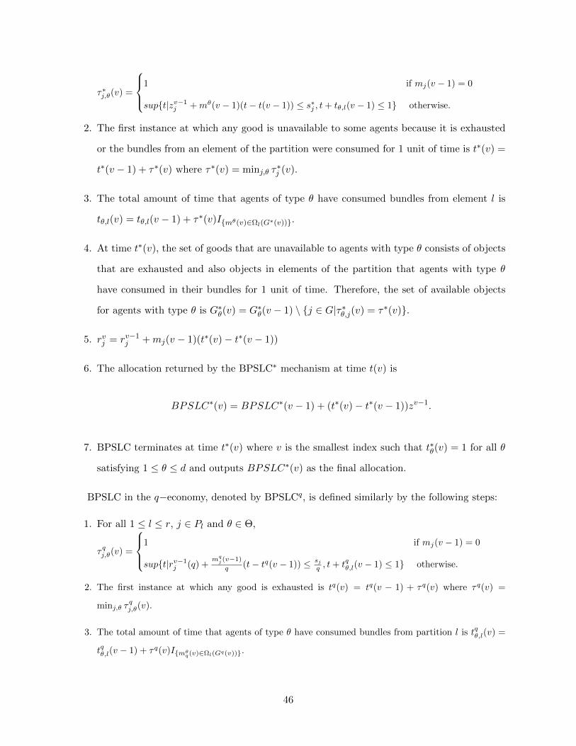
τ∗j,θ(v) =
1 if mj(v − 1) = 0
supt|zv−1j +mθ(v − 1)(t− t(v − 1)) ≤ s∗j , t+ tθ,l(v − 1) ≤ 1 otherwise.
2. The first instance at which any good is unavailable to some agents because it is exhausted
or the bundles from an element of the partition were consumed for 1 unit of time is t∗(v) =
t∗(v − 1) + τ∗(v) where τ∗(v) = minj,θ τ∗j (v).
3. The total amount of time that agents of type θ have consumed bundles from element l is
tθ,l(v) = tθ,l(v − 1) + τ∗(v)Imθ(v)∈Ωl(G∗(v)).
4. At time t∗(v), the set of goods that are unavailable to agents with type θ consists of objects
that are exhausted and also objects in elements of the partition that agents with type θ
have consumed in their bundles for 1 unit of time. Therefore, the set of available objects
for agents with type θ is G∗θ(v) = G∗θ(v − 1) \ j ∈ G|τ∗θ,j(v) = τ∗(v).
5. rvj = rv−1j +mj(v − 1)(t∗(v)− t∗(v − 1))
6. The allocation returned by the BPSLC∗ mechanism at time t(v) is
BPSLC∗(v) = BPSLC∗(v − 1) + (t∗(v)− t∗(v − 1))zv−1.
7. BPSLC terminates at time t∗(v) where v is the smallest index such that t∗θ(v) = 1 for all θ
satisfying 1 ≤ θ ≤ d and outputs BPSLC∗(v) as the final allocation.
BPSLC in the q−economy, denoted by BPSLCq, is defined similarly by the following steps:
1. For all 1 ≤ l ≤ r, j ∈ Pl and θ ∈ Θ,
τ qj,θ(v) =
1 if mj(v − 1) = 0
supt|rv−1j (q) +
mqj (v−1)
q (t− tq(v − 1)) ≤ sjq , t+ tqθ,l(v − 1) ≤ 1 otherwise.
2. The first instance at which any good is exhausted is tq(v) = tq(v − 1) + τ q(v) where τ q(v) =
minj,θ τqj,θ(v).
3. The total amount of time that agents of type θ have consumed bundles from partition l is tqθ,l(v) =
tqθ,l(v − 1) + τ q(v)Imθq(v)∈Ωl(Gq(v)).
46

4. At time t∗(v), the set of goods that are unavailable to agents with type θ consists of objects that
are exhausted and also objects in elements of the partition that agents with type θ have consumed
their bundles for 1 unit of time. Therefore, the set of available objects for agents with type θ is:
Gqθ(v) = Gqθ(v − 1) \ j ∈ G|τ qθ,j(v) = τ q(v).
5. rvj (q) = rv−1j (q) +
mqj (v−1)
q (tq(v)− tq(v − 1)).
6. BPSLCq(v) = BPSLCq(v − 1) + (tq(v)− tq(v − 1))zv−1(q)
7. BPSLC terminates at time tq(v) where v is the smallest index such that tqθ(v) = 1 ∀θ ∈ Θ and
outputs BPSLCq(v) as the final allocation.
D.1 Convergence of BPSLCq to BPSLC∗
We first prove the result with the following assumption:
nqθ = 0 for all large enough q and θ such that n∗θ = 0 (30)
As the supply of multiple objects can become unavailable to some agents at the same time,
the set t∗(1), t∗(2), t∗(3), ..., t∗(v∗) will contain some duplicates. Let the distinct values in the
set t∗(1), t∗(2), t∗(3), ..., t∗(v∗) be t1, t2, ..., tg and ordered so that t1 < t2 < t3 < ... < tg.
Set t∗(vi) = ti. Note g may not be equal to v∗. Let Ahθ ⊆ G be the set of objects that became
unavailable to agents with type θ at time th in the BPSLC∗ mechanism. Let sqj(t) and s∗j (t) be the
supply of object j at time t in BPSLCq and BPSLC∗, respectively. Also, assume BPSLC∗(t)
and BPSLCq(t) are the allocations of the BPSLC algorithm at time t in the continuum economy
and the q−economy, respectively. Denote by θql (t) and θ∗l (t) the times when agents with type θ
have consumed bundles from partition l at time t. We prove the following by induction on h:
1. For all 1 ≤ h ≤ g and all j ∈ G, limq→∞sqj (th)
q = s∗j (th).
2. For all 1 ≤ h ≤ g, 1 ≤ l ≤ r and 1 ≤ θ ≤ d, limq→∞ θql (th) = θ∗l (th).
3. For all 1 ≤ h ≤ g, limq→∞BPSLCq(th) = BPSLC∗(th).
47

For h = 1, note that at the beginning, since all objects are available, all agents are allocated
their most preferred bundle. Therefore, t1 = maxminj∈Gs∗j (0)
mj(G) , 1. Note that for all j ∈ G, the
supply of object j at time t1 in BPSLCq is maxsqj(0)− t1mqj(G), 0. Hence,
limq→∞
sqj(0)− t1mqj(G)
q= s∗j (0)− t1mj(G) = s∗j (t1) = lim
q→∞
maxsqj(0)− t1mqj(G), 0
q.
This proves the base case of the induction.
Assume statements 1, 2, and 3 are true for h− 1; we prove them for h. For all ε > 0, we show
there exists a large enough Q > 0 such that for all q > Q, 1 ≤ θ ≤ d and 1 ≤ l ≤ r:
|sqj(th)
q− s∗j (th)| < ε and |θ∗l (th)− θql (th)| < ε.
Given ε1, let Q1 be such that
|sqj(th−1)
q− s∗j (th−1)| < ε1 and |θ∗l (th−1)− θql (th−1)| < ε1 (31)
for all q > Q1, j ∈ G, 1 ≤ θ ≤ d and 1 ≤ l ≤ r. If object j became unavailable to agents with type
θ at time tτ for some τ < h, then under the BPSLCq mechanism, either these agents can only
consume bundles that include object j for ε1 period of time after th−1 or the availability of object
j at time th−1 is at most ε1q. If the latter is the case, then this object will be allocated for at most
ε1qϑq period of time, where ϑq = minθ∈Θ n
qθ. Note ϑq = O(q). Let ϑ∗ = limq→∞
qϑq . Let Q2 be such
that qε1ϑq ≤ 2ϑ∗ε1 = ε2 for all q > Q2. Choose ε1 such that ε1 + ε2 = ε1(2ϑ∗ + 1) < th − th−1. For
all q > maxQ1, Q2, the BPSLC mechanism in the q−economy at th−1 + ε1 + ε2 would allocate
the same bundles as BPSLC∗. This allocation would end when a good becomes unavailable to
some agents; call this date τ qh . This date is within the ε1 + ε2 neighborhood of
τ qh = min mina∈G∗(vh−1)
sqa(th−1)
mqa(G∗(vh−1))
+ th−1,mint|θql (th−1) + t− th−1 ≥ 1, mθ(G∗(v)) ∈ Ωl(G∗(v)),
where mθ(A) is type θ’s most preferred bundle from the set A. Note that the following holds:
i) mint|θl(th−1) + t− th−1 ≥ 1 ≥ th by definition and limq→∞ θql (th−1) = θl(th−1).
ii) Also note that limq→∞sqj (th−1)
mqa(G∗(vh−1))=
s∗a(th−1)m∗j (G∗(vh−1)) .
48

iii) th =
minmina∈G∗(vh−1)s∗a(th−1)
m∗a(G∗(vh−1)) + th−1,mint|θ∗l (th−1) + t− th−1 ≥ 1, mθ(G∗(v)) ∈ Ωl(G∗(v)). Hence,
for ε3 > 0 there existsQ3 such that for all q > Q3, |τ qh−th| < ε3. Therefore, if q > maxQ1, Q2, Q3,
then |τ qh − th| < ε1 + ε2 + ε3. Note that if q > maxQ1, Q2, Q3, then BPSLCq and BPSLC∗
allocate the same bundles in the interval of [th−1, th] except for a period with length at most
ε1 + ε2 + ε1 + ε2 + ε3. Hence,
|sqj(th)
q− s∗j (th)| ≤ k(ε1 + ε2 + ε1 + ε2 + ε3)|N q|
q. (32)
Since limq→∞|Nq |q exists, choosing εis small enough for this case proves the inductive steps.
In the case that (30) does not hold, the proof follows from the fact that if there is a small
measure o(q) of agents added to the economy, since (as the proof shows) the stock of objects in
the q−economy at all times is either O(q) or o(q), the date at which objects are exhausted stays
the same in the limit.
49


![arXiv:1708.05211v1 [cs.CV] 17 Aug 2017Hung Vuy, Dinh Phungy, Tu Dinh Nguyeny, Anthony Trevorszand Svetha Venkateshy yCentre for Pattern Recognition and Data Analytics (PRaDA) School](https://static.fdocuments.net/doc/165x107/5ed52cb795d1070c2d72a44d/arxiv170805211v1-cscv-17-aug-2017-hung-vuy-dinh-phungy-tu-dinh-nguyeny-anthony.jpg)


