Asset Pricing Models and Industry Sorted Portfolios
28
1 Asset Pricing Models and Industry Sorted Portfolios Author: Marijn de Vries ANR: 264141 Faculty: Faculty of Economics and Business studies Programme: Bedrijfseconomie Supervisor: Jiehui Hu MSc Date: 7/6/2012
Transcript of Asset Pricing Models and Industry Sorted Portfolios
1
Asset Pricing Models and Industry Sorted Portfolios
Author: Marijn de Vries
ANR: 264141
Faculty: Faculty of Economics and Business studies
Programme: Bedrijfseconomie
Supervisor: Jiehui Hu MSc
Date: 7/6/2012

2
Table of Contents
I. Introduction .................................................................................................................. 3
II. Theoretical background ................................................................................................. 5
Modern portfolio theory ................................................................................................... 5
Capital Asset Pricing Model ............................................................................................... 6
CAPM anomalies ............................................................................................................... 7
Fama- French Three Factor Model ..................................................................................... 7
Fama- French- Carhart Model ............................................................................................ 8
Pricing industry portfolios.................................................................................................. 9
III. Data ......................................................................................................................... 11
IV. Methodology ........................................................................................................... 13
V. Empirical results .......................................................................................................... 15
VI. Conclusions ............................................................................................................. 18
References .......................................................................................................................... 20
Appendix ............................................................................................................................. 22

3
I. Introduction
Over time, many different models have been developed that help explain the return on
stocks by looking at risk factors. The basis for many of these models lies in the
Capital Asset Pricing Model (Sharpe, 1964/ Lintner, 1965) which was developed in
the early sixties. This model was in turn based on earlier work by Markowitz (1952),
in which he presented his Modern Portfolio Theory. In the following decades, many
different researchers have tried to extend the basic CAPM. They have tried to further
specify the different risk factors that help to explain stock returns in order to make the
model even more powerful and reliable. Two of these newer asset pricing models are
the Fama- French Three Factor Model (FF3) and the Fama- French- Carhart Four
Factor Model (FFC). While these later models tend to explain a larger portion of the
variation found in stock returns over long periods of time, they may not necessarily
perform better when we look at short time periods with extraordinary economic
conditions such as a financial crisis. We suspect that even though all of the before
mentioned models are specified correctly for the long time periods, problems may
arise due to redundancy of some of the variables used in the FF3 and FFC models as a
result of a temporary shift in risk loadings, as well as multicolinearity for the Credit
Crunch period. This suspicion is based on the fact that the extra variables used in the
FF3 and FFC models are not true risk factors: they were added to the CAPM model in
order to explain certain empirically observed anomalies and are therefore proxies for
one or more true risk factors. If some of these proxies measure the aggregated risk
that results from several true risk factors in different proportions then a temporary
shift in weights of true risk factors could cause the proxies to become highly
correlated. Another problem that has become apparent from previous research is the
fact that accurately pricing assets on an industry level causes problems when we use
the CAPM or FF3 asset pricing models (Fama& French, 1997, Moerman, 2005).
These papers report a drop in the R2 as well as an increase in the pricing error for
some regressions when the models are applied to industry based portfolio returns. It
seems that the usefulness of the variables in these models is not the same for all
industries; Fama and French (1997) speculate that this is due to uncertainty about the
true risk factors, as well as the shifts in risk loadings that occur over time. The degree
in which industry returns are sensitive to changes in risk loadings may not be the same

4
for all industry portfolios. If this is indeed the case then studying the differences
between industries could lead to a better understanding of the underlying true risk
factors of the proxy variables used in the FF3 and FFC models, which in turn could
lead to a better explanation of the variation in stock returns. While some research has
been done on the application of the FF3 and CAPM models on industry sorted
portfolios, we have yet to find a paper that also looks at the results for the FFC model.
The research that was done on industry portfolio pricing with the use of these models
is scarce and often inconclusive. So, in this paper we will try to address the following
questions: 1) can all three models be used to explain the variation in stock returns both
for the long term, as well as the Credit Crunch period, and 2) which of these models
provides the greatest benefits when we apply them to industry based portfolios for
both the 10 year period as well as the crisis period in terms of explaining power, fit
and reliability? In order to answer these questions we will use a data set consisting of
daily industry portfolio returns as well as the daily risk factors and risk free interest
rates for the period 2001-2010, which we acquired from the website of Kenneth
French. In our analyses we will focus on regressions for the whole 10 year period, as
well as a sub period for the credit crunch crisis which consists of data from 12-01-
2007 to 06-01-2009. In the first part of this paper we will take a closer look at the
three models and their theoretical background. We will then proceed with a
description of the dataset and methodology we used and finally we present our
findings which we will try to link back to the theory discussed below.

5
II. Theoretical background
Modern portfolio theory
As we have already mentioned before, the basis for the CAPM and other subsequent
models can be found in the Modern Portfolio Theory as described by Markowitz
(1952). In the formulation of this theory Markowitz used two important assumptions
about investor behavior. The first assumption is that all investors (should) strive to
maximize the expected return on their investments. The second assumption is that
investors will try to keep the variance, or fluctuation, of these expected returns as low
as possible. The first makes sense; an investor should always try to get the most profit
from his investment. But the actual profit for a certain holding period is not fixed for
most investments because of uncertainty in cash flows and discount rates. So we can
only base our portfolio selection on estimated-, or expected returns. But regardless of
the discount rates we use for different assets and the change of these discount rates
over time, an investor will always choose to invest all his wealth in the asset with the
highest discounted value. This would imply that investors have no use for
diversification. But if we add the second assumption; the need for investors to keep
the variance of the expected returns as low as possible for a given expected return, a
new picture emerges. Why would an investor choose to invest in a portfolio that has
huge variances in the returns over a portfolio that has a much more gradual return if
the average returns are exactly the same? The answer is quite simple: he doesn‟t. He
will try to maximize the expected return of his portfolio and at the same time
minimize the variance of the expected returns. Markowitz combined these two
important facts and shows that the covariance between different assets can be used to
lower (or increase) the variance in expected returns. This means that by diversifying
the portfolio, an investor can lower the risk while keeping the expected return of the
total investment constant. This approach leads to the formation of well diversified
efficient portfolios based on the investor‟s preferred combination of expected return
and variance. It gives investors the opportunity to maximize profits while, at the same
time, minimizing the risk associated with the investment.

6
Capital Asset Pricing Model
The CAPM model as described by Sharpe (1964) and Lintner (1965) builds on
Markowitz‟s Modern Portfolio Theory. The fact that diversification can be used to
reduce the variance of expected returns for a portfolio of assets is applied to the
market as a whole. All investors will try to attain a portfolio that maximizes the
expected return and at the same time minimizes the risk associated with holding the
portfolio. The only way they can do this is by buying and selling assets. In doing so,
the price of the assets change and therefore the expected return changes. This process
results in an efficient frontier for all investors; the assets that comprise an efficient
portfolio may change over time, but the minimum amount of risk that needs to be
incurred to attain a certain expected return is the same for all investors. This means
that in a state of equilibrium there will be a simple linear relation between risk and
return for any efficient combination of risky assets in the market. Sharp and Lintner
show that, in their model, the correlation between the efficient market portfolio and all
other assets is caused by their common dependence on the general state of the
economy. If this is true then investors could diversify all risk with the sole exception
of the risk associated with the overall level of economic productivity or systematic
risk. This means that when we assess the risk of an asset only the sensitivity of the
asset to systematic risk matters. Because of this, asset prices will continue to change
until there is a linear relationship between the expected return of an asset and its
sensitivity to systematic risk. So in the CAPM there is only one risk factor: an asset‟s
expected return depends only on the exposure of the asset to the overall market risk.
So the expected return of asset i can be found by adding the risk free interest rate to
the expected excess market return multiplied by the sensitivity of asset i to this
market:
E[Ri]=rf + ßi(E[Rm]-rf)
From this we can construct the Security Market Line, this is the graphical
representation of the linear relation between all assets ß‟s and expected returns. If the
CAPM holds then all assets should fall on this line in the equilibrium state. This was
used by Black, Jensen& Scholes (1972). By measuring α, the distance that the actual
7
returns lie above or below the SML prediction for the expected return, they argued
that if the CAPM was right then α should never be significantly different from 0 for
longer periods of time.
CAPM anomalies
Black, Jensen& Scholes (1972) found that there was indeed a portion of stock returns
that could not be explained by the Capital Asset Pricing Model. In other words; α was
significantly different from 0 for groups of stocks during certain time periods. And
they were not alone in finding discrepancies between the CAPM expected returns and
real world stock returns. For instance, Banz (1981) found that small firms (measured
by total market capitalization) had higher risk adjusted returns than large firms. In
addition, Fama& French (1988/1992) found that not only size, but also the book-to-
market ratio of a firm helps to explain its stock returns. While both size and BE/ME
ratio can be used to explain a part of the expected returns of a stock, they are firm
characteristics and not risk factors. Fama& French (1993,1995) argue that both of
these firm characteristics are a measure of (future) profitability; they found that stocks
with a low BE/ME ratio are more profitable than stocks with a high BE/ME for a
period of 4 years before and 5 years after the raking was made. Low BE/ME is
characteristic for firms with a high average return on equity (growth stocks) and a
high BE/ME ratio signals low earnings compared to equity (often a signal of financial
distress). This financial distress can be explained by a number of causes, for instance
firm inefficiency, high levels of (involuntary) leverage, or cash flow problems
(Chan& Chen, 1991). Furthermore, companies with a low market capitalization tend
to have lower earnings on book equity than stocks with a high market capitalization
(Fama& French, 1992, 1995). So while BE/ME ratios and size by themselves are not
risk factors, they do seem to be good proxies for risk factors than can help explain a
stock‟s expected return.
Fama- French Three Factor Model
The observed anomalies in the stock market returns from previously mentioned
research led to the addition of two new risk factors to the original CAPM (Fama&
French 1992, 1993, 1995, 1997). These factors were constructed by forming portfolios

8
based on company size and BE/ME- ratio. The first was a risk factor that corrects for
the size effect (SMB), measured by the relative market capitalization. The second was
a factor that accounts for the previously unexplained differences in the variance of
returns of growth and value stocks (HML). This model became known as the Fama-
French Three Factor Model (FF3):
E[Ri]=rf + bi(E[Rm]-rf) + siSMB + hiHML
The addition of these two new risk factors provided a significant increase in the R2
while at the same time lowering the pricing error |α|. However, the method used by
Fama and French to construct the SMB and HML portfolios was also subject to
criticism. Kothari, Shanken and Sloan (1995) argue that the COMPUSTAT data used
by Fama and French was subject to a survivor bias, especially the data on small stocks
with a high BE/ME ratio could be affected because small, financially distressed
companies could have been delisted from the stock market (for instance because of
bankruptcy or low trading volumes) before they were added to the compustat dataset
that was used to form the portfolios. Fama and French (1995) address these concerns;
their first remark is that the survivor bias problem is much smaller for their research
because they use value weighted returns instead of the equal weighted returns used by
Kothari, Shanken and Sloan (1995). They also argue that this bias problem does not
apply to the large firms: even when the bottom half of the size sorted data is dropped,
the high BE/ME stocks still outperform the low BE/ME stocks. But their most
important argument is that the fact that small stocks with high BE/ME ratios do not
survive only reinforces their evidence that these stocks have persistent low earnings.
Fama- French- Carhart Model
The third and last model that we will be using in this paper is the Fama- French-
Carhart model (FFC). This model builds on the FF3- model by adding a momentum
risk factor. This risk factor is included in order to explain the one year momentum
anomaly found by Jegadeesh and Titman (1993). They found that the returns of
portfolios based on prior performance of individual assets yields abnormal returns. At
first these abnormal returns were explained as market inefficiency caused by a lag in
the reaction to new information on stocks (Chan, Jegadeesh& Lakonishok, 1995). But
the fact that this momentum anomaly is persistent over time (Jegadeesh& Titman,
9
1993) and is found in various countries (Asness, Liew& Stevens, 1997), suggest that
there is a common risk factor that can explain this momentum anomaly. Carhart
(1997) compares this new expanded model with the CAPM and FF3 and shows that
the addition of a momentum factor significantly lowers the average pricing error when
these models are applied to portfolios that are sorted on their prior year‟s
performance. Furthermore, he reports that the FFC risk factor loadings are not
substantially affected by multicollinearity. This suggests that the new momentum
factor explains a part of the variation in stock returns that is not captured by the risk
factors in the CAPM and FF3 models.
Pricing industry portfolios
The CAPM, FF3 and the FFC models perform relatively well when used on the (US)
stock market as a whole. When these models are used to evaluate returns of
portfolio‟s based on industry, this changes. Research has show that accurately pricing
assets on an industry level causes problems (Fama& French, 1997, Moerman, 2005).
Both the CAPM and FF3 models show a reduction in R2 as well as an increase in |α|
when they are applied to industry based portfolio returns. In addition, the estimated
cost of equity (CE) becomes imprecise. The standard errors for the CE become more
than three percent for both models, so when the models are used to form a prediction
interval for the cost of equity using a one-standard-error bounded interval the interval
becomes quite large which makes it practically useless (Fama& Fench, 1997). We can
illustrate this with an example: if we would have an annualized market return of 4 %
and a standard error of 3% for this premium, then the one- standard- error bounds for
the CE of an investment opportunity with a beta of 1 would be 1% for the lower
bound and 7% for the upper bound. The two-standard-error bounds would become
-2% and 10%. Because these intervals are so large, accurately estimating the
profitability of an investment becomes almost impossible. Furthermore, the estimates
of the CAPM and FF3 differ more than two percent for many industries (Fama&
Fench, 1997). These differences are likely driven by uncertainty about true risk
factors and imprecise estimates of period-by-period risk loadings (Fama& Fench,
1997). This uncertainty in the prediction of the CE causes problems for companies
when these CE estimates are used to evaluate investment opportunities; an error in the
estimated CE could cause the rejection of profitable investments or, even worse, the
10
acceptance of projects with a negative NPV. The ability to accurately estimate the CE
is therefore of vital importance when making finance decisions.
It is suggested in previous literature that the SMB and HML factors could be related
to a firm‟s relative financial distress. As we have mentioned before, inefficient firms
(relative inefficient use of capital, for instance inefficient production lines) with high
leverage and cash flow problems, seem to drive the small firm effect according to
Chan & Chen (1991). Furthermore, Fama and French (1992) speculate that the
premium associated with high book equity to market equity (BE/ME) might be due to
the risk of financial distress. This is supported by results from Fama and French
(1994), which shows that industry sorted portfolios experience periods of growth and
distress and that the HML loading is not constant over time. While there is no hard
theoretical evidence that conclusively proves that size and book-to-market factors
proxy for financial distress, some recent studies that focused on industry based
portfolio returns for US (Fama & French, 1994), UK (Hussain& Toms, 2002) and
European markets (Moerman, 2005) report similar results in different markets which
suggests that the SMB and HML proxies could be related to a true risk factor that
measures financial distress. The rationale behind this link is that some industries are
affected more strongly by economy wide changes that take place during business
cycles than others, thus causing increased industry growth or increasing the risk of
financial distress for certain industries while others remain relatively unaffected. If
this is indeed the case and the SMB and HML factors are able to capture (a portion of)
this industry dependent systematic risk, the FF3 model should clearly outperform the
CAPM both in terms of R2 and |α| when these models are applied to industry sorted
portfolio returns. Furthermore we would expect to see a large shift in the risk
loadings for these factors for cyclical industries during the Credit Crunch period
compared to the whole time period, while non-cyclical industries risk loadings should
remain relatively unaltered. As industries experience growth and distress through
various periods of time, industry risk may have an idiosyncratic element that is
specific to the industry for a period of time causing under or over-reaction to the
market (Hussain & Toms, 2002).

11
III. Data
In this paper we will be using a long time series of daily average value weighted
industry returns data based on all companies listed on the NYSE, AMEX and
NASDAQ for which the relevant data was available during the period January 2001 to
December 2010. These returns, as well as the industry definitions which can be found
in the appendix, were retrieved from Kenneth French‟s website. The 10 industries
were defined using the first four digits of the stocks sic codes. We also retrieved the
four daily risk factors from Kenneth French‟s website, as well as the daily risk free
interest rate for the 10 year period.
The daily excess industry returns were computed by subtracting the risk-free rate from
the daily return of each industry. We also created a dummy variable for the Credit
Crunch period: Dcrisis=1 for the period 12-01-2007 to 06-01-2009. This period is based
on the NBER US Business Cycle Expansions and Contractions reports and captures
the period in which the first shock of the credit crunch caused a contraction in the US
economy. Even though this time period is not directly based on the stock market
returns, it covers the height of the effects of the crisis on the US stock market. This
enables us to compare the performance of the different models during „normal‟ times
and the Credit Crunch period. Furthermore, it encompasses enough observations for
making statistical inferences.
The methods used to construct our risk factors can be found in Fama and French
(1992, 1993, 1996), Griffin (2002), Moerman (2005) and Carhart(1997). While we
did not construct these risk factors for this particular paper, but instead used the risk
factors provided by Kenneth French, we still feel it is important to describe how they
were constructed for completeness of this paper.
Firstly, all stocks are ranked on market capitalization (size). The sample median is
calculated and the sample is split into two groups; one portfolio of companies with a
large market capitalization (L), the other with small market capitalization (S). The
sample is also sorted on the BE/ME ratio. The top 30% form the high book-to-market
portfolio (H), the middle 40% the middle portfolio (M), and the bottom 30% is the
low book-to-market portfolio (L). Six combinations are then formed: SL, SM, SH,

12
BL, BM, BH. The SMB is the simple average of all small (S) portfolio returns minus
big (B) portfolio returns:
SMB= (SL+SM+SH-BL-BM-BH)/3
And the HML is constructed by taking the average of the high BE/ME portfolio
returns minus the low BE/ME portfolio returns for each month:
HML= (BH+SH-SL-BL)/2
To construct the momentum factor six value weighted portfolios were created on size
and 11 months prior returns. These six portfolios are formed from the intersections of
the 2 size sorted stocks, and 3 prior 11 months return sorted portfolios. The three prior
return portfolios are defined as the top 30%, middle 40% and bottom 30%. The
momentum risk factor can then be calculated by taking the average return on the two
high prior return portfolios minus the average return of the two low prior return
portfolios:
MOM=(SH+BH-SL-BL)/2

13
IV. Methodology
We will start by performing an OLS regression of the three different models on daily
excess stock returns on the whole data set (all industries). The regression models that
we will be using are as follows:
Rit-Rft = αi+βi[Rmt-Rf]+eit
Rit-Rft = αi+bi[Rmt-Rft]+siSMBt+hiHMLt+eit
Rit-Rft = αi+bi[Rmt-Rft]+siSMBt+hiHMLt+ miMOMt+eit
With:
Rit= return of portfolio i on month t
Rft= risk-free rate in month t
Rmt= market return in month t
βi, bi, si, hi, mi = unconditional sensitivities of asset i for respective risk factor
αi= pricing error
eit= error term
And SMB, HML and MOM are returns of the value-weighted, zero-investment,
factor-mimicking portfolios for size, book-to-market equity and prior returns. We will
use the regression results to provide a benchmark for both R2 and |α| for all three
models, using F- tests to determine if the regressions as a whole are statistically
significant and t-tests to check if any of the variables used in the regressions are
insignificant. The pricing error will be checked to determine if it is significantly
different from zero using t-statistics. This is in line with previous research Fama and
French (1992, 1993, 1996).
The second step is to perform these same regressions for just the crisis period. We
will then try to determine if any of these models are incorrectly specified for this
particular period. Because if this is indeed the case then we cannot accurately explain
stock returns for the crisis period using that particular model. We will check for
multicolinearity using correlation matrices and variance inflation factors for the

14
independent variables (VIF). The regression results of the models that survive these
tests can then be compared to the regression results for the whole ten year period. We
make this comparison to see if a shift in the sensitivity to the different risk factors can
be found. And again, the R2 and |α| will be recorded and α will be tested to see if it is
significantly different from zero.
The last step is to zoom in on the industry based portfolio‟s and, using the results from
the previous tests, determine which of the three different models is most suited to
explain the returns. Furthermore, we want to determine if the shift in sensitivities to
the different risk factors as observed from the whole dataset regression is consistent
with the shifts observed on industry level.
15
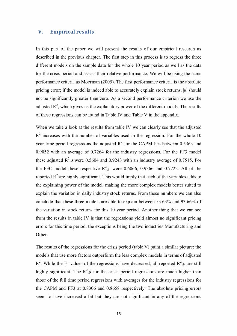
V. Empirical results
In this part of the paper we will present the results of our empirical research as
described in the previous chapter. The first step in this process is to regress the three
different models on the sample data for the whole 10 year period as well as the data
for the crisis period and assess their relative performance. We will be using the same
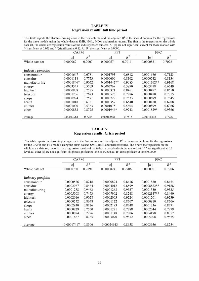
performance criteria as Moerman (2005). The first performance criteria is the absolute
pricing error; if the model is indeed able to accurately explain stock returns, |α| should
not be significantly greater than zero. As a second performance criterion we use the
adjusted R2, which gives us the explanatory power of the different models. The results
of these regressions can be found in Table IV and Table V in the appendix.
When we take a look at the results from table IV we can clearly see that the adjusted
R2 increases with the number of variables used in the regression. For the whole 10
year time period regressions the adjusted R2 for the CAPM lies between 0.5363 and
0.9052 with an average of 0.7264 for the industry regressions. For the FF3 model
these adjusted R2„s were 0.5604 and 0.9243 with an industry average of 0.7515. For
the FFC model these respective R2„s were 0.6066, 0.9366 and 0.7722. All of the
reported R2 are highly significant. This would imply that each of the variables adds to
the explaining power of the model, making the more complex models better suited to
explain the variation in daily industry stock returns. From these numbers we can also
conclude that these three models are able to explain between 53.63% and 93.66% of
the variation in stock returns for this 10 year period. Another thing that we can see
from the results in table IV is that the regressions yield almost no significant pricing
errors for this time period, the exceptions being the two industries Manufacturing and
Other.
The results of the regressions for the crisis period (table V) paint a similar picture: the
models that use more factors outperform the less complex models in terms of adjusted
R2. While the F- values of the regressions have decreased, all reported R2„s are still
highly significant. The R2„s for the crisis period regressions are much higher than
those of the full time period regressions with averages for the industry regressions for
the CAPM and FF3 at 0.8306 and 0.8658 respectively. The absolute pricing errors
seem to have increased a bit but they are not significant in any of the regressions
16
performed. So the models seem to explain a larger portion of the variation in stock
returns for the crisis period than for the whole 10 year period. But when we look at
Table VI we can see a problem; for the whole period the correlations between the
variables used in the three different models seems to lie within a reasonable range, but
the correlation matrix for the crisis period subset indicates that a multicollinearity
problem arises for the momentum factor used in the FFC model. This is confirmed
when we look at the VIF value for the momentum factor which is 3.32. The
momentum factor seems to have an unacceptably high correlation with the HML
factor for this time period. These two factors seem to explain, for a large part, the
same variation in returns. This could indicate that the FFC model is not correctly
specified for the crisis period, making it less suitable to explain the variation in returns
for this period even though it performs well in terms of R2 and Jensen‟s Alpha.
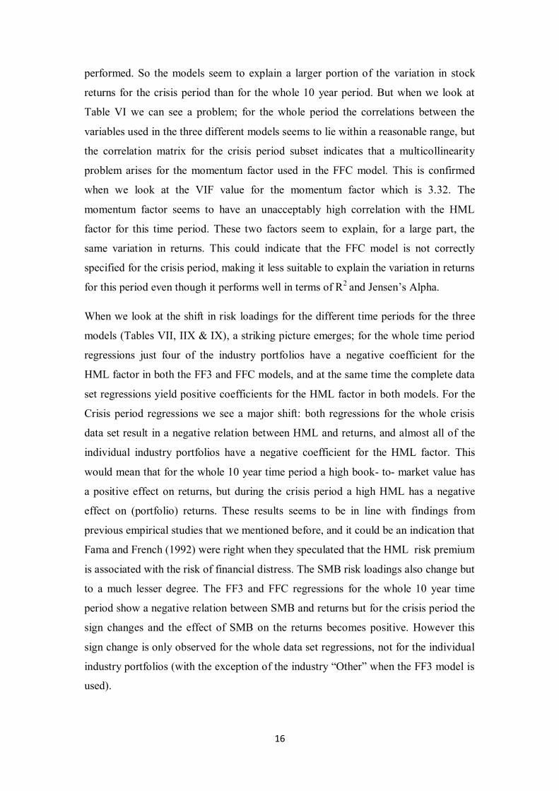
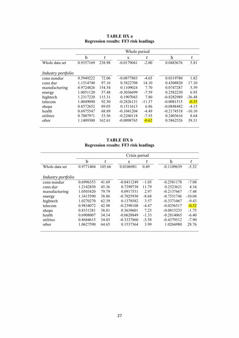
When we look at the shift in risk loadings for the different time periods for the three
models (Tables VII, IIX & IX), a striking picture emerges; for the whole time period
regressions just four of the industry portfolios have a negative coefficient for the
HML factor in both the FF3 and FFC models, and at the same time the complete data
set regressions yield positive coefficients for the HML factor in both models. For the
Crisis period regressions we see a major shift: both regressions for the whole crisis
data set result in a negative relation between HML and returns, and almost all of the
individual industry portfolios have a negative coefficient for the HML factor. This
would mean that for the whole 10 year time period a high book- to- market value has
a positive effect on returns, but during the crisis period a high HML has a negative
effect on (portfolio) returns. These results seems to be in line with findings from
previous empirical studies that we mentioned before, and it could be an indication that
Fama and French (1992) were right when they speculated that the HML risk premium
is associated with the risk of financial distress. The SMB risk loadings also change but
to a much lesser degree. The FF3 and FFC regressions for the whole 10 year time
period show a negative relation between SMB and returns but for the crisis period the
sign changes and the effect of SMB on the returns becomes positive. However this
sign change is only observed for the whole data set regressions, not for the individual
industry portfolios (with the exception of the industry “Other” when the FF3 model is
used).

17
If we consider the individual industries we find that the there are several industries for
which the three models seem to perform above average. The industries are
Manufacturing, Hightech and Other. The regressions for these industries yield high
R2„s for all three models for both the 10 year time period as well as the crisis period.
However, if we look at the 10 year period we also find that the industries
Manufacturing and Other are the only ones that produce significant (albeit small)
pricing errors. So ironically, the industries for which the models used in this paper
seem to explain the variation in daily returns best in terms of R2 also seem to hint at
the existence of pricing errors. When we look at the FF3 regression results for these
industries for the crisis period we find that these are the only two industries for which
the coefficient for the HML factor has a positive sign.
18
VI. Conclusions
Based on our results we find that while all three models can be used to explain returns
for the whole ten year period, a multicolinearity problem arises if we apply the FFC
model to the crisis period returns. The momentum factor that is used in the FFC
model becomes highly correlated with the HML factor. While the problem does not
seem to be severe, the gains in terms of R2 when including the momentum factor in
the regressions are small compared to the results generated by the reduced model
(FF3). This becomes especially clear when we compare the momentum risk loadings
for the whole time period to the crisis period risk loadings for the whole data set
regressions. The coefficient of the momentum variable drops from 0.0643282 for the
10 year period to 0.0074445 during the crisis period. This could be an argument to use
the FF3 model instead of the FFC model for this particular period.
The regressions of the industry based portfolio returns provide us with some
interesting results: the industries that perform best in terms of R2 (Manufacturing and
Other) are also the only two industries for which the regressions yielded significant
pricing errors. Furthermore the Manufacturing and Other industry portfolios are the
only two that have a positive risk loading for the HML factor in the FF3 regressions
for the crisis period. So even though the models are able to explain a large part of the
variation in daily excess returns for these two industry portfolios, there is still a
significant pricing error present. The fact that these two industries are the only two for
which the HML risk loadings do not change from positive to negative also raises
questions. It would seem that these two industries in particular are especially
interesting for further research, especially concerning the underlying risk factor(s) of
the HML proxy.
Both the FF3 and the FFC models rely on proxies for true risk factors. Even though
the use of these proxies improves the results of the regressions they also create
problems, especially when we apply these models to industry based portfolios. The
multicolinearity found in the FFC model for the crisis period is just one example of
this. However, the shift in risk loadings observed for HML and SMB for nearly all
industries during the crisis period could be an indication that these variables are

19
proxies one or more true risk factors that measure financial distress as suggested by
Fama and French (1992) which is not included in the CAPM model.
The results of our research clearly illustrate the need for further research into the true
underlying risk factors of the SMB, HML and UMD variables that are used in the FF3
and FFC models. Looking at industry portfolios could be a good starting point for this
research. Comparing the results of the application of these models to industry
portfolios and the “real world” differences between the industries could lead to
important insights into the theoretical risk factors that affect assets returns.

20
References Asness, C. S., Liew, J. M., & Stevens, R. L. (1997). Parallels Between the Cross-Sectional Predictability of Stock and Country Returns. The Journal of Portfolio Management, 23(3), 79-87 doi: 10.3905/jpm.1997.409606 Carhart, M. M. (1997). On Persistence in Mutual Fund Performance. The Journal of Finance, 52(1), 57-82. Chan, K. C., & Chen, N.-F. (1991). Structural and Return Characteristics of Small and Large Firms. The Journal of Finance, 46(4), 1467-1484. Chan, L. K. C., Jegadeesh, N., & Lakonishok, J. (1995). Momentum Strategies. National Bureau of Economic Research Working Paper Series, No. 5375. Fama, E. F., & French, K. R. (1988a). Dividend yields and expected stock returns. Journal of Financial Economics, 22(1), 3-25. doi: 10.1016/0304-405x(88)90020-7 Fama, E. F., & French, K. R. (1988b). Permanent and Temporary Components of Stock Prices. Journal of Political Economy, 96(2), 246-273. Fama, E. F., & French, K. R. (1992). The Cross-Section of Expected Stock Returns. The Journal of Finance, 47(2), 427-465. Fama, E. F., & French, K. R. (1993). Common risk factors in the returns on stocks and bonds. Journal of Financial Economics, 33(1), 3-56. doi: 10.1016/0304-405x(93)90023-5 Fama, E. F., & French, K. R. (1994). Industry costs of equity. Working paper, Graduate School of Business, University of Chicago, Chicago, IL, revised July 1995 Fama, E. F., & French, K. R. (1995). Size and Book-to-Market Factors in Earnings and Returns. The Journal of Finance, 50(1), 131-155. Fama, E. F., & FrencH, K. R. (1996). Multifactor Explanations of Asset Pricing Anomalies. The Journal of Finance, 51(1), 55-84. Fama, E. F., & French, K. R. (1997). Industry costs of equity. Journal of Financial Economics, 43(2), 153-193. doi: 10.1016/s0304-405x(96)00896-3 Fama, E. F., & French, K. R. (2004). The Capital Asset Pricing Model: Theory and Evidence. The Journal of Economic Perspectives, 18(3), 25-46. doi: 10.1257/0895330042162430 Griffin, J. M. (2002). Are the Fama and French Factors Global or Country Specific? Review of Financial Studies, 15(3), 783-803. doi: 10.1093/rfs/15.3.783 Hussain, S. I., & Toms, S. (2002). Industry Returns, Single and Multifactor Asset Pricing Tests. SSRN eLibrary. doi: 10.2139/ssrn.302694 Jegadeesh, N., & Titman, S. (1993). Returns to Buying Winners and Selling Losers: Implications for Stock Market Efficiency. The Journal of Finance, 48(1), 65-91.

21
Jensen, M. C., Black , F., & Scholes, M. S. (1972). The Capital Asset Pricing Model: Some Empirical Tests. Michael C. Jensen, STUDIES IN THE THEORY OF CAPITAL MARKETS, Praeger Publishers Inc., 1972. Kothari, S. P., Shanken, J., & Sloan, R. G. (1995). Another Look at the Cross-Section of Expected Stock Returns. The Journal of Finance, 50(1), 185-224. Lessard, D. R. (1974). World, National, and Industry Factors in Equity Returns. The Journal of Finance, 29(2), 379-391. Liew, J., & Vassalou, M. (2000). Can book-to-market, size and momentum be risk factors that predict economic growth? Journal of Financial Economics, 57(2), 221-245. doi: 10.1016/s0304-405x(00)00056-8 Lintner, J. (1965). The Valuation of Risk Assets and the Selection of Risky Investments in Stock Portfolios and Capital Budgets. The Review of Economics and Statistics, 47(1), 13-37. Markowitz, H. (1952). Portfolio Selection. The Journal of Finance, 7(1), 77-91. Moerman, G. A. (2005). How Domestic is the Fama and French Three-Factor Model? An Application to the Euro Area. SSRN eLibrary. Moskowitz, T. J., & Grinblatt, M. (1999). Do Industries Explain Momentum? The Journal of Finance, 54(4), 1249-1290. doi: 10.1111/0022-1082.00146 Post, T., & Van Vliet, P. (2004). Do Multiple Factors Help or Hurt? SSRN eLibrary. doi: 10.2139/ssrn.582101 Rolf W, B. (1981). The relationship between return and market value of common stocks. Journal of Financial Economics, 9(1), 3-18. doi: 10.1016/0304-405x(81)90018-0 Sharpe, W. F. (1964). Capital Asset Prices: A Theory of Market Equilibrium under Conditions of Risk. The Journal of Finance, 19(3), 425-442.

22
Appendix
TABLE I Industry definitions
This table provides an overview of the industry classifications used in this paper and the sic codes used in their formation. Industry number
Industry name Description Sic codes
1 Consumer nondurables
Food, Tobacco, Textiles, Apparel, Leather, Toys 0100-0999 2000-2399 2700-2749 2770-2799 3100-3199 3940-3989
2 Consumer durables
Cars, TV's, Furniture, Household Appliances 2500-2519 2590-2599 3630-3659 3710-3711 3714-3714 3716-3716 3750-3751 3792-3792 3900-3939 3990-3999
3 Manufacturing Machinery, Trucks, Planes, Chemicals, Off Furn, Paper, Com Printing
2520-2589 2600-2699 2750-2769 2800-2829 2840-2899 3000-3099 3200-3569 3580-3621 3623-3629 3700-3709 3712-3713 3715-3715 3717-3749 3752-3791 3793-3799 3860-3899
4 Energy Oil, Gas, and Coal Extraction and Products 1200-1399 2900-2999
5 Hitech Business Equipment -- Computers, Software, and Electronic Equipment and related services
3570-3579 3622-3622 3660-3692 3694-3699 3810-3839 7370-7372 7373-7373 7374-7374 7375-7375 7376-7376 7377-7377 7378-7378 7379-7379 7391-7391 8730-8734
6 Telecom Telephone and Television Transmission 4800-4899 7 Shops Wholesale, Retail, and Some Services (Laundries,
Repair Shops) 5000-5999 7200-7299 7600-7699
8 Health Healthcare, Medical Equipment, and Drugs 2830-2839 3693-3693 3840-3859 8000-8099
9 Utilities Utilities 4900-4949 10 Other Other -- Mines, Constr, BldMt, Trans, Hotels, Bus
Serv, Entertainment, Finance other

23
TABLE II Sample breakdown by industry and fiscal year
This table provides a breakdown of the dataset to the number of observations per industry per year. Industry/ year 01 02 03 04 05 06 07 08 09 10 total cons nondur 248 252 252 252 252 251 251 253 252 251 2514 cons dur 248 252 252 252 252 251 251 253 252 251 2514 manufacturing 248 252 252 252 252 251 251 253 252 251 2514 energy 248 252 252 252 252 251 251 253 252 251 2514 hightech 248 252 252 252 252 251 251 253 252 251 2514 telecom 248 252 252 252 252 251 251 253 252 251 2514 shops 248 252 252 252 252 251 251 253 252 251 2514 health 248 252 252 252 252 251 251 253 252 251 2514 utilities 248 252 252 252 252 251 251 253 252 251 2514 other 248 252 252 252 252 251 251 253 252 251 2514 Total 2480 2520 2520 2520 2520 2510 2510 2530 2520 2510 25140
24
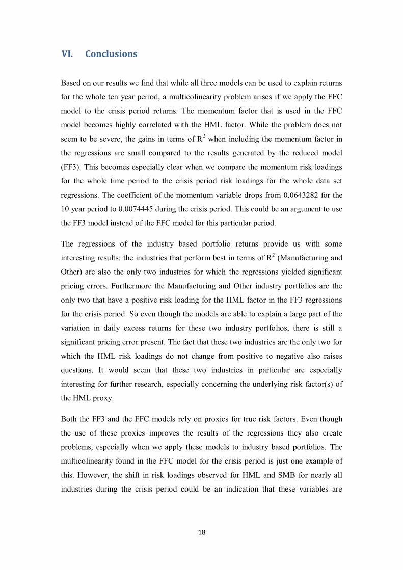
Table III Descriptive statistics
This table provides descriptive statistics for all variables, returns and risk free interest rate measured in daily percentages. Variable Description T Mean Median St.dev. Min. Max. Industry level variables cons nondur Value weighted excess return for industry 1 2514 0.0002428 0.00043 0.0099166 -0.06883 0.10277 cons dur Value weighted excess return for industry 2 2514 0.0002671 0.000555 0.0184493 -0.11659 0.09767 manufacturing Value weighted excess return for industry 3 2514 0.0003128 0.000725 0.0140912 -0.09783 0.10747 energy Value weighted excess return for industry 4 2514 0.0004881 0.00084 0.0184962 -0.15483 0.19327 hightech Value weighted excess return for industry 5 2514 0.0000730 0.000875 0.0184637 -0.08597 0.16014 telecom Value weighted excess return for industry 6 2514 0.0000106 0.00032 0.0156566 -0.09673 0.14507 shops Value weighted excess return for industry 7 2514 0.0002041 0.000365 0.0134201 -0.08223 0.10987 health Value weighted excess return for industry 8 2514 -0.0000126 0.000245 0.011673 -0.06713 0.11087 utilities Value weighted excess return for industry 9 2514 0.0001938 0.00085 0.0133835 -0.08923 0.14427 other Value weighted excess return for industry 10 2514 0.0000698 0.000215 0.0172931 -0.12434 0.1126
market variables RF Risk free rate 2514 0.0000852 0.00007 0.0000699 0 0.00026 E_RETURN Value weighted Excess market return 2514 0.0001310 0.0007 0.0136953 -0.09 0.1152 SMB Size risk factor 2514 0.0002374 0.0004 0.0059244 -0.038 0.0431 HML BE/ME risk factor 2514 0.0002001 0.0002 0.0064512 -0.0487 0.0403 UMD Momentum risk factor 2514 0.0000141 0.0007 0.0113879 -0.0829 0.071
Other variables CRISIS =1 if observation is between 12-1-2007 and 6-1-
2009 2514 0.1578529 0.1578529 0.3646103 0 1
25
TABLE IV Regression results: full time period
This table reports the absolute pricing error in the first column and the adjusted R2 in the second column for the regressions for the three models using the whole dataset SMB, HML, MOM and market returns. The first is the regression on the whole data set, the others are regression results of the industry based subsets. All |α| are not significant except for those marked with *(significant at 0.05) and **(significant at 0.1). All R2 are significant at 0.0000. CAPM FF3 FFC |𝛼| 𝑅2 |𝛼| 𝑅2 |𝛼| 𝑅2 Whole data set Industry portfolio
0.000062 0.7007 0.000057 0.7011 0.0000531 0.7028
cons nondur 0.0001647 0.6781 0.0001793 0.6812 0.0001686 0.7123 cons dur 0.0001118 0.7753 0.0000606 0.8102 0.0000542 0.8134 manufacturing 0.0001846* 0.9052 0.0001442** 0.9083 0.0001362** 0.9168 energy 0.0003545 0.5709 0.0003769 0.5890 0.0003478 0.6549 hightech 0.0000808 0.7585 0.0000321 0.8461 0.0000477 0.8650 telecom 0.0001206 0.7673 0.0000523 0.7786 0.0000470 0.7815 shops 0.0000924 0.7571 0.0000729 0.7633 0.0000699 0.7645 health 0.0001018 0.6381 0.0000357 0.6540 0.0000450 0.6708 utilities 0.0001000 0.5363 0.0001075 0.5604 0.0000899 0.6066 other 0.0000852 0.8775 0.0001946* 0.9243 0.0001829* 0.9366 average
0.00013964
0.7264
0.00012561
0.7515
0.00011892
0.7722
TABLE V Regression results: Crisis period
This table reports the absolute pricing error in the first column and the adjusted R2 in the second column for the regressions for the CAPM and FF3 models using the crisis dataset SMB, HML and market returns. The first is the regression on the whole crisis data set, the others are regression results of the industry based subsets. |α| marked with ** are significant at 0.1 level, all other |α| are not significant (highest significance level is 0.355), all R2 are significant at level 0.0000. CAPM FF3 FFC |𝛼| 𝑅2 |𝛼| 𝑅2 |𝛼| 𝑅2 Whole data set Industry portfolio
0.0000730 0.7891 0.0000824 0.7906 0.0000901 0.7906
cons nondur 0.0000526 0.8218 0.0000894 0.8416 0.0001850 0.8454 cons dur 0.0002067 0.8464 0.0004012 0.8899 0.0008822** 0.9188 manufacturing 0.0001288 0.9463 0.0001268 0.9537 0.0001350 0.9535 energy 0.0005508 0.7473 0.0007902 0.8248 0.0012147** 0.8460 hightech 0.0002016 0.9028 0.0002063 0.9224 0.0001201 0.9239 telecom 0.0000552 0.8648 0.0001122 0.8707 0.0000810 0.8706 shops 0.0002930 0.8126 0.0002193 0.8348 0.0001236 0.8371 health 0.0000829 0.7560 0.0001271 0.7788 0.0002744 0.7879 utilities 0.0000074 0.7296 0.0001148 0.7806 0.0004198 0.8057 other 0.0001627 0.8785 0.0003070 0.9612 0.0005008 0.9655 average
0.00017417
0.8306
0.00024943
0.8658
0.0003936
0.8754

26
TABLE VI Correlations
Correlations for full dataset Correlations for crisis dataset
Ri-Rf Rm-Rf SMB HML MOM Ri-Rf Rm-Rf SMB HML MOM Ri-Rf 1 Ri-Rf 1
Rm-Rf 0.8371 1 Rm-Rf 0.8884 1
SMB 0.0114 0.0233 1 SMB -0.1158
-0.1342 1
HML 0.1477 0.1522 -0.0551 1 HML 0.4413 0.5349 -
0.0695 1
MOM -0.3820
-0.4962 0.0639 -
0.1504 1 MOM -0.5965
-0.6937
-0.0033
-0.7567 1
TABLE VII Regression results: CAPM risk loadings
Whole period Crisis period ß t ß t Whole data set Industry portfolio
0.9390052 242.60 0.9494793 121.88
cons nondur 0.5963323 72.77 0.6384909 42.75 cons dur 1.1862170 93.12 1.2401500 46.73 manufacturing 0.9789569 154.93 0.9936059 83.55 energy 1.0205740 57.83 1.1913790 34.23 hightech 1.1742450 88.85 0.9378859 60.67 telecom 1.0014820 91.04 0.9887557 50.33 shops 0.8527014 88.52 0.7955514 41.45 health 0.6809142 66.57 0.6250143 35.04 utilities 0.7157597 53.92 0.7775130 32.70 other 1.1828700 134.17 1.3064460 53.52
27
TABLE IIX a
Regression results: FF3 risk loadings
Whole period b 𝑡 s 𝑡 h 𝑡 Whole data set Industry portfolio
0.9357169 238.98 -0.0179041 -2.00 0.0483676 5.81
cons nondur 0.5949222 72.06 -0.0877883 -4.65 0.0319780 1.82 cons dur 1.1514740 97.16 0.3822708 14.10 0.4308820 17.10 manufacturing 0.9724826 154.54 0.1109024 7.70 0.0747287 5.59 energy 1.0051120 57.48 -0.3036699 -7.59 0.2582230 6.95 hightech 1.2317220 115.31 0.1907043 7.80 -0.8282989 -36.48 telecom 1.0049090 92.50 -0.2826131 -11.37 -0.0081515 -0.35 shops 0.8572652 89.05 0.1511613 6.86 -0.0848482 -4.15 health 0.6975547 68.89 -0.1041204 -4.49 -0.2174518 -10.10 utilities 0.7007971 53.56 -0.2260118 -7.55 0.2403616 8.64 other 1.1409300 162.61 -0.0098765 -0.62 0.5862526 39.31
TABLE IIX b Regression results: FF3 risk loadings
Crisis period b 𝑡 s 𝑡 h 𝑡 Whole data set Industry portfolio
0.9771404 105.66 0.0106981 0.49 -0.1109639 -5.52
cons nondur 0.6996353 41.69 -0.0411249 -1.05 -0.2581178 -7.08 cons dur 1.2142850 45.36 0.7399738 11.79 0.2523621 4.34 manufacturing 1.0503420 79.79 0.0917531 2.97 -0.2137667 -7.48 energy 1.3415590 38.86 -0.7025930 -8.68 -0.7531746 -10.04 hightech 1.0270270 62.39 0.1378582 3.57 -0.3371067 -9.43 telecom 0.9834072 42.98 -0.2398108 -4.47 -0.0256517 -0.52 shops 0.8331281 38.81 0.3638601 7.23 -0.0815233 -1.75 health 0.6908007 34.14 -0.0628849 -1.33 -0.2814065 -6.40 utilities 0.8684615 34.03 -0.3337860 -5.58 -0.4379512 -7.90 other 1.0627590 64.65 0.1537364 3.99 1.0266980 28.76

28
TABLE IX a
Regression results: FFC risk loadings
Whole period b 𝑡 s 𝑡 h 𝑡 m 𝑡 Whole data set Industry portfolio
0.961757 215.11 -0.0267175 -2.98 0.0565854 6.80 0.0643282 11.95
cons nondur 0.6671090 72.28 -0.1122204 -6.23 0.0547589 3.27 0.1783268 16.50 cons dur 1.1083100 82.35 0.3968799 14.71 0.4172603 16.65 -0.1066297 -6.58 manufacturing 1.0262800 149.56 0.0926942 6.74 0.0917064 7.18 -0.1328994 16.09 energy 1.2011030 65.47 -0.3700043 -10.06 0.3200745 9.37 0.4841682 21.93 hightech 1.1269200 98.37 0.2261754 9.85 -0.8613729 -40.37 -0.2589001 -18.78 telecom 0.9691745 78.44 -0.2705185 -10.92 -0.0194288 -0.84 -0.0882776 -5.94 shops 0.8771873 79.78 0.1444186 6.55 -0.0785611 -3.84 0.0492145 3.72 health 0.7602049 67.22 -0.1253247 -5.53 -0.1976805 -9.38 0.1547682 11.37 utilities 0.8195960 57.83 -0.2662200 -9.37 0.2778525 10.53 0.2934755 17.20 other 1.0616850 144.43 0.0169443 1.15 0.5612443 40.99
-0.1957627 -22.13
TABLE IX b Regression results: FFC risk loadings
Crisis period b 𝑡 s 𝑡 h 𝑡 m 𝑡 Whole data set Industry portfolio
0.9799050 89.26 0.0124732 0.57 -0.1031551 -3.95 0.0074445 0.47
cons nondur 0.7342678 37.32 -0.0188870 -0.48 -0.1602939 -3.42 -0.0932610 3.27 cons dur 1.0399360 38.11 0.6280246 11.47 -0.2401095 -3.70 -0.4695010 -11.86 manufacturing 1.0473730 66.96 0.0898466 2.86 -0.2221534 -5.97 -0.0079955 -0.35 energy 1.4954440 38.93 -0.6037844 -7.84 -0.3185059 -3.48 0.4143944 7.44 hightech 0.9957733 51.84 0.1177906 3.04 -0.4253855 -9.24 -0.0841612 -3.00 telecom 0.9720846 35.77 -0.2470810 -4.53 -0.0576337 -0.89 -0.0304903 -0.77 shops 0.7984554 31.55 0.3415968 6.73 -0.1794607 -2.98 -0.0933694 -2.54 health 0.7442005 31.65 -0.0285970 -0.61 -0.1305718 -2.33 0.1437993 4.22 utilities 0.9790195 34.35 -0.2627968 -4.60 -0.1256656 -1.85 0.2977196 7.20 other 0.9924956 53.97 0.1086202 2.94 0.8282287 18.92
-0.1892117 -7.09


![Class 8 The Capital Asset Pricing Model. Efficient Portfolios with Multiple Assets E[r] 0 Asset 1 Asset 2 Portfolios of Asset 1 and Asset 2 Portfolios.](https://static.fdocuments.net/doc/165x107/56649e505503460f94b4758c/class-8-the-capital-asset-pricing-model-efficient-portfolios-with-multiple.jpg)