ASSET PRICING AND THE CREDIT MARKET

Francis A. Longstaff Jiang WangUCLA Anderson School MIT Sloan School,and NBER CCFR, and NBER

Abstract

We study asset pricing and trading behavior in an exchange economy populated by two agentswith different risk aversion. We show that the credit market plays a central role in the risk sharingbetween the two agents. It allows the less-risk-averse agent to borrow in order to take on leveredpositions in the stock and thus bear more risk. Optimal risk sharing results in the more-risk-averseagent effectively selling covered “call” options to the less-risk-averse agent. As the state of theeconomy changes, the equilibrium amount of credit in the market also fluctuates, which in turninfluences expected stock returns, stock return volatility, the term structure of interest rates, andtrading activity in the stock market. We further explore the immediate empirical implication thatvariation in the size of the credit market is related to variation in expected stock returns. Usingvarious measures of changes in the size of the credit market, we find that they have significantpower in forecasting one-year excess returns of the stock market. Our results suggests that thecredit sector is of fundamental importance to the behavior of asset prices.

First draft: November 2007. Current draft: April 2008.

The authors are grateful for helpful discussions with John Cochrane, Jun Liu, Hanno Lustig, andPedro Santa-Clara, for excellent research assistance from Dongyan Ye, and for comments fromseminar participants at the FDIC.

1. INTRODUCTION

The simple representative-agent setting has become one of the most-popular models for studyingequilibrium asset pricing (e.g., Lucas (1978) and Cox, Ingersoll and Ross (1985)). In such a setting,the credit market plays only a virtual role. For the representative agent, equilibrium borrowing andlending, which equals the aggregate supply of credit, is always zero. Hence, models with only onerepresentative agent are largely silent about quantity variables in the market and their connectionwith prices. In particular, they make no predictions about the actual behavior of the credit sectorand how it influences asset pricing.

In reality, however, the credit sector plays a central role in the financial markets. Recent eventssuch as the subprime-mortgage crisis and the subsequent liquidity shocks in the financial marketsindicate that the availability of credit (or the lack thereof) can have first-order effects on assetprices. Thus, introducing a meaningful credit sector into the standard asset-pricing framework is anatural extension that might provide new insights about the workings of financial markets.

Using a model similar to Wang (1996), we extend the canonical asset-pricing framework toallow for two classes of investors, each with a different level of risk aversion. In this setting, the twoclasses of investors borrow from and lend to each other. This results in a significant credit sectorthat expands and contracts in response to shocks to the economy. We solve the model in closedform and provide explicit solutions for equilibrium prices and investors’ optimal consumption andtrading strategies. We then examine the role of the credit market and its connection with assetprices. Especially, we explore how the amount of credit, determined endogenously in the market,facilitates risk sharing among investors and influences the behavior of stock and bond prices.

A number of interesting results emerge from this analysis. First, we show that the equilibriumconsumption allocation between the two agents, each being the representative investor of his class,is such that the more-risk-averse agent’s consumption is less risky than the aggregate endowment(or consumption) while the less-risk-averse agent’s consumption is more risky. As a result, the more-risk-averse agent ends up with the lion’s share of total consumption in bad states of the economy(when aggregate consumption is low) while giving up much of his share in the good states. Such anallocation is equivalent to the more-risk-averse agent selling a covered “call” option on the aggregateendowment or the stock market to the less-risk-averse agent, shifting more risk from the former tothe latter. Trading activity in the model is driven by the dynamic replication strategies associatedwith these convex option-like consumption allocations.

Second, the credit market is essential in facilitating this optimal risk sharing. In particular,the more-risk-averse agent provides liquidity in the form of credit to the less-risk-averse agent,allowing him to take on levered positions in the stock and thus bear more risk. In return, themore-risk-averse agent switches part of his portfolio into debt, receiving a stream of safe cash flowsin the form of interest payments. As a result, the size of the credit market varies drastically withmarket “demographics,” i.e., the wealth distribution between the two agents. When the wealth istoo skewed toward one agent, which is the case when the economy is in extremely good or badstates, the credit market becomes minuscule. This is because the agent with little wealth can nolonger accommodate the borrowing or lending needs of the other agent. For intermediate states ofthe economy, however, the size of the credit market becomes substantial, allowing sufficient leveragefor the less-risk-averse agent to take on more risk.

Moreover, we show that the relative size of the credit market is closely related to the behaviorof asset prices. Under calibrated parameter values, we find that stock return volatility comoves

1

with the market’s leverage ratio, defined as the total amount of credit in the market normalized bythe total size of the market. This is in part because as leverage reaches its maximum, agents’ wealthand consumption shares become most sensitive to changes of the economy, which leads to morevolatile stock prices. In fact, we show that when both agents are present, despite the expandedrisk-sharing opportunities provided by the credit and stock market, the equilibrium stock pricevolatility can be higher than its level when only one of the agents is present. In addition, we findthat when the leverage ratio is maximized, the interest rate becomes more stable, which also leadsto an overall upward-sloping term structure for interest rates.

Furthermore, we show that under i.i.d. shocks to the economy, the resulting market demo-graphics, shaped by agents’ risk-sharing strategies, evolve in non-trivial ways. This leads to richpatterns in stock and bond returns. For example, the dividend yield, risk premium, and Sharperatio of the stock typically behave countercyclically. In extremely bad states of the economy, how-ever, the stock’s risk premium can turn procyclical, becoming negatively correlated with dividendyield. Under certain parameter values, the dividend yield and the expected return of the stock canboth be nonmonotonic with respect to the level of the market and behave procyclically. The stockreturns also displays interesting forms of heteroscedasticity. The volatility is highly persistent overtime, procyclical in low states of the economy but countercyclical in high states.

A key contribution of the paper is to establish a fundamental link between asset prices andquantities in the market, especially the amount of credit. The primary empirical implication ofthe model is that changes in the size of the credit sector are highly informative about shifts in thedemographics of the market, which, in turn, drive the behavior of asset prices. More specifically,changes in the size of the credit sector should be linked to time variation in the equity premium.Thus, information about the size of the credit market may prove useful in forecasting excess stockreturns.

We test this empirical implication using the standard predictive regression framework familiarfrom the asset-pricing literature. Specifically, we regress one-year (nonoverlapping) excess returnson the CRSP value-weighted index for the 1953 to 2006 period on a number of variables thatprevious research has suggested may have predictive ability for excess stock returns: lagged stockreturns, the dividend yield, and Lettau and Ludvigson’s (2001) cay measure. We then introduceseveral measures of the size of the credit sector into the regression and examine how the predictiveability of the regression changes.

The results are striking. By themselves, the lagged stock return, dividend yield, and cayvariables result in a predictive regression for the one-year horizon with an adjusted R2 of about17 percent. When the credit sector variables are introduced, however, the adjusted R2 for theregression increases to over 40 percent. These levels of predictability for stock returns are farhigher than any previously documented in the literature. These results demonstrate both thetheoretical and empirical importance of the credit sector in asset-pricing models.

Several papers have considered the impact of heterogeneity in investors’ risk aversion on assetpricing. Dumas (1989) and Wang (1996) use a two-agent setting to examine how heterogeneitygives rise to time-varying risk aversion in the aggregate and the resulting behavior of interest rates.Further allowing the feature of “catching-up with the Joneses” in investor preferences in a similarsetting, Chan and Kogan (2002) consider the dynamics of stock prices.

Our paper extends this line of research in three important directions. First, while these papersfocus on the behavior of prices, we focus on both prices and quantities, especially the interactionbetween the two. To link prices with quantities is of essential importance to models with hetero-

2

geneous investors—it is where these models can produce new, distinctive, and testable predictionsbeyond those from a representative model. After all, in a complete market, there always exists arepresentative-agent model for an economy with heterogeneous agents that yields identical pricingrelations from the fundamentals. Thus, empirical tests of these models have to turn to the addi-tional predictions, which must concern disaggregated variables such as quantities. By solving andanalyzing in closed-form investors’ portfolio behavior together with prices, we are able to producevarious predictions directly connecting the two. Next, we explore some of the empirical predictionsof the model. In particular, we show that the amount of credit endogenously generated in the mar-ket contains useful information about the risk premium of the stock. Another important feature ofour paper is its analysis of the credit market, in particular, how the amount of credit is related tothe degree of risk sharing and the resulting stock and bond prices. In addition, even with limiteddegrees of freedom, we are able to produce a rich set of results concerning both the dynamics ofstock and bond prices that are compatible with the empirical findings, at least for some sets ofcalibrated parameters.

This paper is organized as follows. Section 2 describes the model. Section 3 presents a single-agent version of the model as a benchmark for comparison. Section 4 solves the equilibrium for thetwo-agent model. Section 5 discusses the equilibrium consumption allocation. Section 6 analyzeshow the credit market helps the two agents achieve the optimal risk sharing. Section 7 examinesthe behavior of asset prices in the model and the interactions with borrowing and lending in thecredit market. Section 8 considers the trading activity in the stock market. Section 9 reports ourexploratory empirical work on the link between the size of the credit market and stock marketreturns. Section 10 concludes the paper. All proofs are provided in the Appendix.

2. THE MODEL

The model used throughout this paper parallels Wang (1996). Specifically, we consider a pureexchange economy in which there is a single perishable consumption good that also serves as thenumeraire. The economy is endowed with a flow of the consumption good. We denote the rate ofendowment flow as Xt and assume that it follows a geometric Brownian motion,

dXt = μ Xt dt + σ Xt dZt, (1)

whereX0 > 0, μ ≥ 0 and σ > 0 are constants, and Zt is a standard Wiener process.1 The processXt

is positive with probability one and, conditional on Xt, Xt+τ with τ ≥ 0 is lognormally distributed.

There exists a market where shares of the aggregate endowment (the “stock”) are traded. Ashare of the stock yields a dividend flow at rate Xt. The total number of shares of the stock inthe economy then equals one. In addition, there exists a “money market” where a locally risklesssecurity is traded (i.e., investors can borrow from or lend to each other without default). As isstandard, we assume that this riskless security is in zero net supply in the economy. Let Pt denotethe price of the stock and rt the instantaneous riskless interest rate.

Investors in this economy can trade competitively in the securities market and consume theproceeds. Let Ct be an investor’s consumption rate, Nt his holdings of the stock, and Mt his

1Throughout the paper, equalities or inequalities involving random variables are always in the senseof almost surely with respect to the underlying probability measure.

3

holdings of the riskless security. The consumption and trading strategies {Ct, (Nt,Mt)} are adaptedprocesses satisfying the standard integrability conditions, that is, ∀ T ∈ [0,∞),∫ T

0

Ct dt < ∞, (2a)

∫ T

0

|Mt rt dt + Nt (Xt dt + dPt) | < ∞, (2b)

∫ T

0

N 2t d[Pt] < ∞, (2c)

where [Pt] denotes the quadratic variation process of Pt.2 The investor’s wealth process, definedby Wt = Mt + Nt Pt, must be positive with probability one, and conform to the stochasticdifferential equation,

dWt = rt Mt dt + (Xt dt + dPt) Nt − Ct dt. (3)

The requirement that wealth be positive is to rule out arbitrage opportunities (following Dybvigand Huang (1988)). Let Θ denote the set of consumption/trading strategies that satisfy the aboveconditions.

There are two classes of identical investors in the economy, denoted as 1 and 2. Both classes areinitially endowed with only shares of the stock. The initial endowment of shares for the classes ofinvestors are 1−n and n, respectively. The initial number of shares optimally chosen by each classat time zero, of course, need not equal their initial endowments. Investors in each class choose theirconsumption and investment strategies to maximize their lifetime expected utility. The preferencesof the two classes of investors are

Et

[∫ ∞

0

e−ρτC1−γ

1,t+τ

1 − γdτ

], (4a)

Et

[∫ ∞

0

e−ρτC1−2γ

2,t+τ

1 − 2γdτ

], (4b)

respectively, where γ is a positive constant. C1,t and C2,t denote the total consumption of the firstand second classes of investors, respectively. Thus, the first and second classes of investors haveconstant relative risk aversion (CRRA) of γ and 2γ, respectively.

We further impose several conditions on the model’s parameter values. The first condition isthe growth condition,

ρ > max {0, (1 − γ)(μ− 12γσ2), (1 − 2γ)(μ− γσ2)}. (5)

It ensures that investors’ expected utilities are uniformly bounded given the aggregate consumptionprocess in Equation (1). In addition, we need the following set of conditions√

(μ− 12σ2)2 + 2ρσ2 + (μ− 1

2σ2) − 2γσ2 > 0, (6a)

√(μ− 1

2σ2)2 + 2ρσ2 − (μ− 1

2σ2) + (γ − 1)σ2 > 0. (6b)

2See Karatzas and Shreve (1988) for a discussion of the quadratic variation process of a givenstochastic process.

4

These conditions guarantee that the stock and bond prices behave properly.3

In specifying the securities markets, we have only introduced the stock and the locally risklesssecurity as traded securities. As will be shown later, the stock and the riskless security are sufficientto dynamically complete the securities market in the sense of Harrison and Kreps (1979). Arbitraryconsumption plans (satisfying certain integrability conditions) can be financed by continuous trad-ing in the stock and the riskless security. Allowing additional securities will not affect the nature ofthe equilibrium. Thus, in deriving the market equilibrium, we will consider the securities marketas consisting of only the stock and the riskless security. Simple arbitrage arguments can then beused to price other securities if they exist.

We have assumed that there are only two classes of investors in the economy and that theybehave competitively in the market. Since investors within each class have the same isoelasticpreferences, we can represent each class with a single representative investor who has the samepreferences as the individual investors and the total endowment of each class (see, for example,Rubinstein (1974)). In deriving the equilibrium, we can then treat the economy as populated withthe two representative investors who behave competitively. In the remainder of the paper, we treatthe two representative investors generically and simply refer to them as the more-risk-averse andless-risk-averse agents.

Market equilibrium in this economy consists of a pair of price processes {Pt, rt} and theconsumption-trading strategies {Ci,t, (Ni,t,Mi,t), i = 1, 2} such that the agents’ expected lifetimeutilities are maximized subject to their respective wealth dynamics in Equation (3), and the secu-rities markets clear:

N1,t + N2,t = 1, (7a)

M1,t + M2,t = 0. (7b)

3. THE SINGLE-AGENT EQUILIBRIUM

Before presenting the results for the two-agent model, we first review the trading and asset-pricingimplications of the familiar single-representative-agent model in our setting. In fact, as shown byStapleton and Subrahmanyam (1990), this is the well-known situation considered by Black andScholes (1973). The results from the single-agent model then provide a benchmark for comparisonto those from the two-agent model.

The single-agent model is nested within the two-agent model by assuming that only one of thetwo agents, say the less-risk-averse agent, is present in the market. Thus, the less-risk-averse agentis initially endowed with all of the shares of stock in the economy, 1 − n = 1 or n = 0.4 The agentmaximizes his expected lifetime utility through consumption and investment choices {Ct, (Nt,Mt)}.3Given CRRA preferences and the process for the aggregate endowment, both agents’ marginalutility and stock payoffs are unbounded from above. Thus, parameter restrictions are needed toensure the prices of certain securities such as the stock and bonds are well defined.4The parallel case where the more-risk-averse agent is endowed with all the shares of stock is givenby simply replacing γ with 2γ throughout all of the formulas in this section.

5

Here, for brevity, we have omitted the subscript i in denoting agent i. In equilibrium, however,the agent’s consumption Ct must equal the aggregate amount of dividends Xt. Similarly, marketclearing implies that the agent holds all of the shares of the stock and does not borrow or lend;Nt = 1 and Mt = 0. This latter feature makes the trading implications of the single-agent modelsimple as there is no trading in equilibrium and the agent never changes the number of shares ofthe stock or the riskless asset in his portfolio.

The equilibrium price of the stock can be obtained directly from the Euler equation associatedwith Nt,

Pt = Et

[∫ ∞

0

e−ρτ

(Ct+τ

Ct

)−γ

Xt+τ dτ

]= XtEt

[∫ ∞

0

e−ρτ

(Xt+τ

Xt

)1−γ

dτ

], (8)

where the second equality follows from Ct = Xt. As shown in the Appendix, this expression reducesto

Pt =1

ρ− κXt, (9)

whereκ = (1 − γ)(μ− 1

2σ2) + 1

2 (1 − γ)2σ2. (10)

Thus, the price-dividend ratio, defined as

Yt = Pt/Xt, (11)

is constant in the single-agent economy, i.e., Yt = 1/(ρ− κ). Its inverse yt = Xt/Pt is simply thedividend yield of the stock, which is ρ− κ.

An application of Ito’s Lemma to Equation (9) gives the dynamics for the stock price,

dPt = Pt (μ dt + σ dZt). (12)

Thus, the stock price inherits the geometric Brownian motion dynamics of the underlying dividendprocess. In this single-agent economy, the agent’s wealth Wt equals the value of his stock holdings,Wt = Mt +NtPt = Pt.

In a similar manner, the riskless rate can be determined from the Euler equation associatedwith Mt. The Appendix shows that the riskless rate is given by

rt = ρ + μγ − 12γ(1 + γ)σ2, (13)

which is a constant.

The single-agent market exhibits some simple properties. For example, the interest rate isconstant and the stock returns are i.i.d. In particular, the expected return on the stock is μ+ yt =μ+ρ−κ and its return volatility is σ, both constant over time. Moreover, stock returns are seriallyuncorrelated. As we see below, these are no longer true when both agents are present in the market.

4. THE TWO-AGENT EQUILIBRIUM

In this section, we present the closed-form solutions for equilibrium consumption, asset prices, andportfolio choices for the two-agent model. We explore the economic intuition and implications of

6

these results more fully in the subsequent sections, and provide the proofs and derivations in theAppendix.

The equilibrium is derived in three steps. First, relying on the complete securities market inour model, we solve for the equilibrium allocation of consumption between the two agents from itsPareto optimality. Second, using the Euler equation for the agents we compute the equilibriumstock price and interest rate that support the equilibrium allocation. Finally, by analyzing theagents’ portfolio policies financing their consumption, we obtain their equilibrium holdings of thestock and the riskless security.

4.1 Consumption

In the two-agent economy, the sum of the agents’ consumption streams must equal the aggregatedividends, i.e. C1,t + C2,t = Xt. An allocation C1,t, C2,t is Pareto optimal if, and only if, thereexists α ∈ [0, 1] such that C1,t, C2,t solves the problem

maxC1,t+C2,t≤Xt

E0

[∫ ∞

0

e−ρt

[αC1−γ

1,t

1− γ+ (1 − α)

C1−2γ2,t

1− 2γ

]dt

]. (14)

The solution is

C1,t = Xt − 2b

(√1 + bXt − 1

), C2,t = Xt −C1,t =

2b

(√1 + bXt − 1

), (15)

where b = 4( α1−α )1/γ. To simplify notation, we denote the more-risk-averse agent’s consumption

simply as Ct. Thus, in equilibrium, the less-risk-averse agent’s consumption is Xt −Ct.

The demographics of the market are characterized by the relative consumption levels of thetwo agents. Let st denote the less-risk-averse agent’s share of total consumption. We have

st =Xt −Ct

Xt=

√1 + bXt − 1√1 + bXt + 1

. (16)

As we will see below, st is an important variable in characterizing the behavior of the economy.We return to analyze its properties in Section 5.

4.2 Asset Prices

Given the equilibrium consumption allocation, we now compute the stock price and the interestrate that support the equilibrium. The Euler equation for the more-risk-averse agent with respectto his stock holding reads

Pt = Et

[∫ ∞

0

e−ρτ

(Ct+τ

Ct

)−2γ

Xt+τ dτ

]. (17)

Substituting the expression for Ct into Equation (17) leads to the following closed-form solutionfor the equilibrium price-dividend ratio of the stock

Pt

Xt= Yt = a1 − a2 st F (1,−θ, 3 + θ − 2γ; st) − a3 (1− st) F (1, λ, 2γ+ 2λ; 1− st), (18)

7

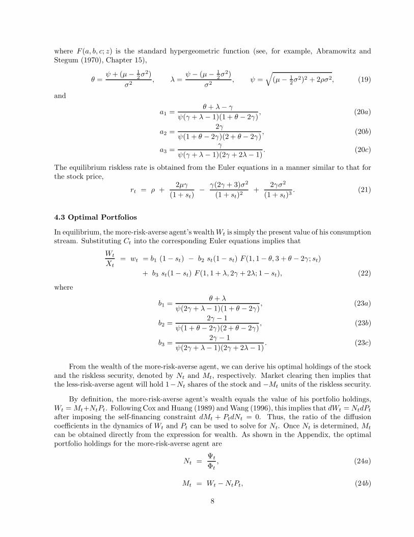
where F (a, b, c; z) is the standard hypergeometric function (see, for example, Abramowitz andStegum (1970), Chapter 15),

θ =ψ + (μ− 1

2σ2)

σ2, λ =

ψ − (μ− 12σ2)

σ2, ψ =

√(μ− 1

2σ2)2 + 2ρσ2, (19)

and

a1 =θ + λ− γ

ψ(γ + λ− 1)(1 + θ − 2γ), (20a)

a2 =2γ

ψ(1 + θ − 2γ)(2 + θ − 2γ), (20b)

a3 =γ

ψ(γ + λ− 1)(2γ + 2λ− 1). (20c)

The equilibrium riskless rate is obtained from the Euler equations in a manner similar to that forthe stock price,

rt = ρ +2μγ

(1 + st)− γ(2γ + 3)σ2

(1 + st)2+

2γσ2

(1 + st)3. (21)

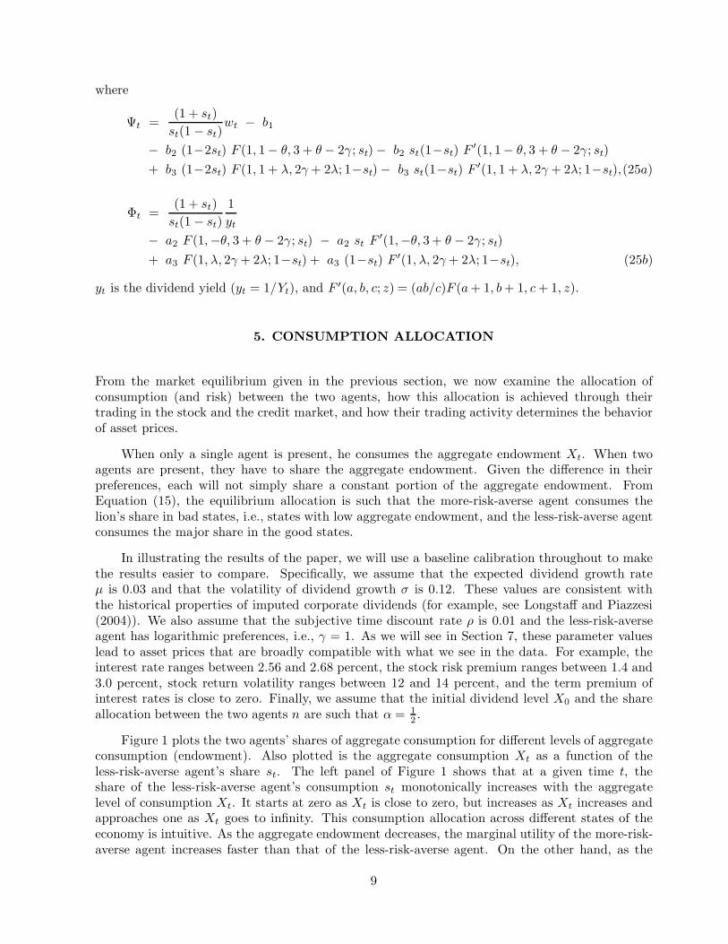
4.3 Optimal Portfolios

In equilibrium, the more-risk-averse agent’s wealthWt is simply the present value of his consumptionstream. Substituting Ct into the corresponding Euler equations implies that

Wt

Xt= wt = b1 (1 − st) − b2 st(1− st) F (1, 1− θ, 3 + θ − 2γ; st)

+ b3 st(1− st) F (1, 1 + λ, 2γ + 2λ; 1− st), (22)

where

b1 =θ + λ

ψ(2γ + λ− 1)(1 + θ − 2γ), (23a)

b2 =2γ − 1

ψ(1 + θ − 2γ)(2 + θ − 2γ), (23b)

b3 =2γ − 1

ψ(2γ + λ− 1)(2γ + 2λ− 1). (23c)

From the wealth of the more-risk-averse agent, we can derive his optimal holdings of the stockand the riskless security, denoted by Nt and Mt, respectively. Market clearing then implies thatthe less-risk-averse agent will hold 1−Nt shares of the stock and −Mt units of the riskless security.

By definition, the more-risk-averse agent’s wealth equals the value of his portfolio holdings,Wt = Mt+NtPt. Following Cox and Huang (1989) and Wang (1996), this implies that dWt = NtdPt

after imposing the self-financing constraint dMt + PtdNt = 0. Thus, the ratio of the diffusioncoefficients in the dynamics of Wt and Pt can be used to solve for Nt. Once Nt is determined, Mt

can be obtained directly from the expression for wealth. As shown in the Appendix, the optimalportfolio holdings for the more-risk-averse agent are

Nt =Ψt

Φt, (24a)

Mt = Wt −NtPt, (24b)

8

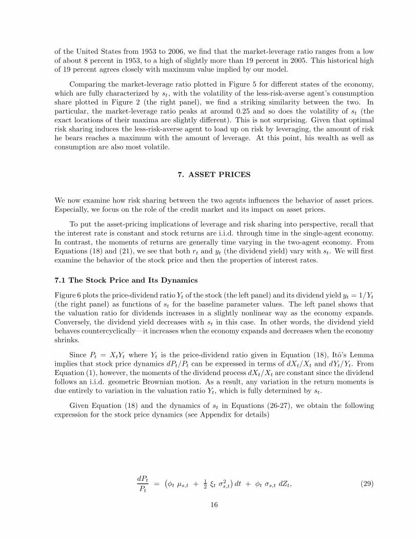
where

Ψt =(1 + st)st(1 − st)

wt − b1

− b2 (1−2st) F (1, 1− θ, 3 + θ − 2γ; st) − b2 st(1−st) F ′(1, 1− θ, 3 + θ − 2γ; st)+ b3 (1−2st) F (1, 1 + λ, 2γ+ 2λ; 1−st) − b3 st(1−st) F ′(1, 1 + λ, 2γ + 2λ; 1−st),(25a)

Φt =(1 + st)st(1 − st)

1yt

− a2 F (1,−θ, 3 + θ − 2γ; st) − a2 st F′(1,−θ, 3 + θ − 2γ; st)

+ a3 F (1, λ, 2γ+ 2λ; 1−st) + a3 (1−st) F ′(1, λ, 2γ+ 2λ; 1−st), (25b)

yt is the dividend yield (yt = 1/Yt), and F ′(a, b, c; z) = (ab/c)F (a+ 1, b+ 1, c+ 1, z).

5. CONSUMPTION ALLOCATION

From the market equilibrium given in the previous section, we now examine the allocation ofconsumption (and risk) between the two agents, how this allocation is achieved through theirtrading in the stock and the credit market, and how their trading activity determines the behaviorof asset prices.

When only a single agent is present, he consumes the aggregate endowment Xt. When twoagents are present, they have to share the aggregate endowment. Given the difference in theirpreferences, each will not simply share a constant portion of the aggregate endowment. FromEquation (15), the equilibrium allocation is such that the more-risk-averse agent consumes thelion’s share in bad states, i.e., states with low aggregate endowment, and the less-risk-averse agentconsumes the major share in the good states.

In illustrating the results of the paper, we will use a baseline calibration throughout to makethe results easier to compare. Specifically, we assume that the expected dividend growth rateμ is 0.03 and that the volatility of dividend growth σ is 0.12. These values are consistent withthe historical properties of imputed corporate dividends (for example, see Longstaff and Piazzesi(2004)). We also assume that the subjective time discount rate ρ is 0.01 and the less-risk-averseagent has logarithmic preferences, i.e., γ = 1. As we will see in Section 7, these parameter valueslead to asset prices that are broadly compatible with what we see in the data. For example, theinterest rate ranges between 2.56 and 2.68 percent, the stock risk premium ranges between 1.4 and3.0 percent, stock return volatility ranges between 12 and 14 percent, and the term premium ofinterest rates is close to zero. Finally, we assume that the initial dividend level X0 and the shareallocation between the two agents n are such that α = 1

2.

Figure 1 plots the two agents’ shares of aggregate consumption for different levels of aggregateconsumption (endowment). Also plotted is the aggregate consumption Xt as a function of theless-risk-averse agent’s share st. The left panel of Figure 1 shows that at a given time t, theshare of the less-risk-averse agent’s consumption st monotonically increases with the aggregatelevel of consumption Xt. It starts at zero as Xt is close to zero, but increases as Xt increases andapproaches one as Xt goes to infinity. This consumption allocation across different states of theeconomy is intuitive. As the aggregate endowment decreases, the marginal utility of the more-risk-averse agent increases faster than that of the less-risk-averse agent. On the other hand, as the

9

0 10 20 30 40 500

0.1

0.2

0.3

0.4

0.5

0.6

0.7

0.8

0.9

1

Aggregate consumption

Con

sum

ptio

n sh

ares

of a

gent

s

0 0.2 0.4 0.6 0.8 10

500

1000

1500

2000

2500

3000

s

Agg

rega

te c

onsu

mpt

ion

Figure 1. Aggregate consumption and agents’ consumption shares. The leftpanel plots the agents’ consumption shares as functions of aggregate consumption, thedashed line for the less-risk-averse agent and the solid line for the more-risk-averse agent,and the right panel plots aggregate consumption as a function of the less-risk-averse agent’sconsumption share st. The parameters are at the benchmark values: μ = 0.03, σ = 0.12,ρ = 0.01, γ = 1.00, and α = 0.50.

aggregate endowment increases, the marginal utility of the more-risk-averse agent decreases fasterthan that of the less-risk-averse agent. The optimal consumption is reached when the marginalutilities of the two agents are equal. This is achieved when the more-risk-averse agent consumesa relatively larger share in the bad states by claiming a relative smaller share in the good states.The right panel of Figure 1 shows that aggregate consumption Xt is very small in absolute valuein the states when the more-risk-averse agent dominates the economy (when st is small), while theopposite is true when the less-risk-averse agent dominates the economy.

Over time, as Xt changes, so does st. In particular, st evolves as follows

dst = μs,t dt + σs,t dZt, (26)

where

μs,t =st(1− st)

1 + st

[(μ− σ2) +

1(1 + st)2

σ2

], (27a)

σs,t =st(1− st)

1 + stσ. (27b)

One immediate observation is that in addition to itself, the dynamics of st depend only on theparameters governing the aggregate consumption process, i.e., μ and σ; the dynamics do not dependon the initial condition of the economy (i.e., X0 and n) which only fixes the initial value of st.More importantly, the dynamics of st do not depend on the parameters concerning the agents’preferences, i.e., ρ and γ. They do, however, depend on the fact that the ratio between the twoagents’ relative risk aversion is two. This property comes from the fact that given the dynamics oftotal consumption, the dynamics of st are determined by the sharing rule between the two agents.

10

Given that the two agents have constant relative risk aversion and the same time discount rate ρ,the sharing rule depends only on the ratio of their relative risk aversion coefficients. In our model,this ratio is two.

The drift and volatility of st imply that it follows a process similar to the class of Wright-Fisher diffusions used in genetics and many other contexts (see, for example, Karlin and Taylor(1981)). The drift of this process is a ratio of simple polynomials. Depending on parameter values,the drift can be uniformly positive (when μ > 3

4σ2), uniformly negative (when μ < 0), or can be

positive for values of st below some threshold and negative for values greater than that threshold(when 0 < μ < 3

4σ2). This latter situation implies a certain type of mean-reverting behavior for

the process. However, the process does not have a stationary distribution in this situation. Thevolatility of the process takes its maximum value at st =

√2 − 1.

0 0.2 0.4 0.6 0.8 1.00

0.0005

0.0010

0.0015

0.0020

0.0025

0.0030

0.0035

0.0040

s

Drif

t of s

0 0.2 0.4 0.6 0.8 1.00

0.005

0.010

0.015

0.020

0.025

s

Vol

atili

ty o

f s

Figure 2. Dynamics of the consumption share of the less-risk-averse agent.The left panel plots the drift of the consumption share of the less-risk-averse agent μs,t

as a function of st and the right panel plots the volatility of the consumption share σs,t.The parameters are at the benchmark values: μ = 0.03, σ = 0.12, ρ = 0.01, and γ = 1.00.

Figure 2 plots both the drift (the left panel) and the volatility of st (the right panel) for the baselineparameter values. Clearly, in this case where μ − 3

4σ2 = 0.03 − 3

4 (0.12)2 = 0.0192 > 0, the driftof st is always positive, indicating that the less-risk-averse agent is steadily gaining share of theeconomy. The drift increases steeply with st for small values of st. It peaks as st approaches 0.4and then declines quickly. The volatility of st has a simple humped shape. It is zero at the twoextreme ends, i.e., when st is equal to zero or one, when one of the agents owns the whole economy.It peaks when st is around 0.4. As we will see below, the dynamics of st are very much related tothe risk sharing between the two agents and the resulting market behavior.

6. RISK SHARING AND THE CREDIT MARKET

The consumption share of the two agents, as shown in Figure 1, reveals a striking pattern. Theconsumption of the less-risk-averse agent is a convex function of aggregate consumption, while

11

that of the more-risk-averse agent is a concave function. This represents the optimal risk sharingbetween the two agents given their preferences. In fact, the more-risk-averse agent shifts a largepart of the aggregate risk, given by the uncertainty in Xt, to the less-risk-averse agent. As a result,the risk profile of the less-risk-averse agent actually exceeds that of the overall economy.

6.1 Leverage and Risk Sharing

Risk sharing is achieved through the two agents’ trading in the securities market. In particular, itis facilitated by the lending of the more-risk-averse agent in the credit market to the less-risk-averseagent. As a result, the more-risk-averse agent is able to switch his stock holdings into riskless debt,thus to maintain a less-risky wealth profile. This is accommodated by the less-risk-averse agent,who issues debt to the more-risk-averse agent to finance his own levered purchase of additionalstock shares.

Thus, the credit market plays a critical role in allowing optimal risk sharing among agentswith different risk preferences. In the absence of a credit market, each of the agents would have tohold the same portfolio consisting of a 100 percent weight in the stock. The presence of the creditmarket allows agents to modify the risk profile of their portfolios by borrowing and lending andthus allocate risk optimally.

0 0.2 0.4 0.6 0.8 1.00

500

1000

1500

2000

2500

3000

s

Bon

d ho

ldin

g of

age

nt tw

o

0 0.2 0.4 0.6 0.8 1.00

0.2

0.4

0.6

0.8

1.0

s

Sto

ck h

oldi

ng o

f age

nt tw

o

Figure 3. Bond and stock holdings of the more-risk-averse agent. The left panelplots the amount of riskless debt the more-risk-averse agent (agent two) holds as a functionof st and the right plots the number of stock shares he holds. The parameters are at thebenchmark values: μ = 0.03, σ = 0.12, ρ = 0.01, and γ = 1.00.

Figure 3 plots the debt and stock shares held by the more-risk-averse agent as a function ofst. The left panel shows Mt, the total amount of “short-term” debt, in the form of instantaneouscredit, held by the more-risk-averse agent. As we can see, for all possible states of the economy(i.e., the whole range of st), Mt is positive. That is, the more-risk-averse agent is always the lenderin the market, lending money to the less-risk-averse agent in exchange for safe future payoffs. Ofcourse, the bond position of the less-risk-averse agent is simply −Mt, which is always negative.

At low levels of Xt, the consumption share of the less-risk-averse agent st is close to zero.

12

In these states, the more-risk-averse agent owns most of the economy and consumes most of theaggregate endowment. As the left panel of Figure 3 shows, the level of debt is small in these statesas the less-risk-averse agent has little wealth to use as collateral in borrowing. As Xt increases,the overall wealth of the economy increases. Moreover, the less-risk-averse agent also has morewealth. Consequently, he can take on more debt by issuing more bonds to the more-risk-averseagent. Indeed, we see that Mt rises quickly with Xt or equivalently st.

While the increase in the lending of the more-risk-averse agent represents a shift in his wealthfrom the stock to bond, the increase in the borrowing of the less-risk-averse agent is used toincrease his stock positions. The right panel of Figure 3 plots the stock shares held by the more-risk-averse agent Nt. Since the total number of stock shares is normalized to one, the numberof shares held by the less-risk-averse agent is simply 1 − Nt. Clearly, at low levels of Xt, themore-risk-averse agent holds most of the stock. In fact, as mentioned above, he owns most of theeconomy and consumes the lion’s share of the aggregate consumption. As Xt increases, however,his stock holding monotonically decreases. When Xt approaches infinity, st approaches one (theless-risk-averse agent consumes most of the economy), and Nt approaches zero. In those states, themore-risk-averse agent holds most of his wealth bonds.

As shown in Cox and Huang (1989), an agent’s portfolio rebalancing can be interpreted as thedynamic trading strategy that generates “derivative” contracts that deliver the optimal consump-tion for each date and state. From this perspective, the portfolio strategy of the more-risk-averseagent, which sells stock shares for bonds as the stock price rises and buys when the stock pricefalls, is exactly to achieve the negative convexity in his desired consumption profile. Thus, throughthe dynamic rebalancing of his stock and bond positions, he is synthetically “selling” call optionsto the less-risk-averse agent. In the vocabulary of the options market, the risk-averse agent is short“gamma,” while the less-risk-averse agent is long “gamma.”

Finding that the risk-averse agent sells options to the less-risk-averse agent may seem coun-terintuitive at first. After all, selling options is generally viewed as a highly risky enterprise. Inthis equilibrium, however, the more-risk-averse agent is not simply selling options outright with apotentially unbounded downside. Rather, the risk-averse agent follows a much more conservative“covered call” strategy by selling options against an underlying stock position. Obviously, thecredit market is crucial to allow him to achieve this through his portfolio strategy.

6.2 Optimal Portfolio Weights

In addition to describing the agents’ stock and bond holdings in absolute terms, we also examinethem in relative terms. In particular, we consider the relative weight of stock in both agents’portfolios wi,t, where

w1,t =(1 −Nt)Pt

(1 −Nt)Pt −Mt, w2,t =

NtPt

NtPt +Mt. (28)

The relative weight of bond in agent i’s portfolio is simply 1−wi,t. Figure 4 plots w1,t and w2,t asa function of st.

Facilitated by the credit market and the possibility of leverage, the difference between the twoagents’ portfolios is striking. For the less-risk-averse agent, the weight of stock in his portfoliois always above one, reflecting the fact that he is always levered. For small values of st, whichcorresponds to low levels of Xt or bad states of the economy, the stock weight in his portfolio isclose to two. In other words, he pledges all his wealth as collateral to borrow. In these states, it is

13

0 0.2 0.4 0.6 0.8 1.01.0

1.2

1.4

1.6

1.8

2.0

s

Por

tfolio

wei

ght o

f sto

ck fo

r ag

ent o

ne

0 0.2 0.4 0.6 0.8 10.5

0.6

0.7

0.8

0.9

1

s

Por

tfolio

wei

ght o

f sto

ck fo

r ag

ent t

wo

Figure 4. Weight of stock in agents’ portfolios. The left panel plots the weightof stock in the portfolio of the less-risk-averse agent (agent one) against st, and the rightpanel plots that of the more-risk-averse agent (agent two). The parameters are at thebenchmark values: μ = 0.03, σ = 0.12, ρ = 0.01, and γ = 1.00.

the more-risk-averse agent who is more wealthy, and he can fully accommodate the leverage needsof the less-risk-averse agent. From Figure 3, we see that the absolute size of debt is small for smallst. But it is a large percentage of the less-risk-averse agent’s portfolio. As st increases, the economymoves into good states, in which the less-risk-averse agent gains a larger share of the total wealth(and consumption). Despite his preference for leverage, less debt would be available as the wealthshare of the more-risk-averse agent dwindles. Consequently, he is forced to reduce leverage and theweight of the stock in his portfolio decreases. When st approaches one, the less-risk-averse agentowns most of the economy, which is the stock. The weight of the stock in his portfolio approachesone.

For the more-risk-averse agent, the weight of stock in his portfolio is always between zero andone since he holds part of his portfolio in the riskless bond. For small values of st (i.e., Xt), he ownsmost of the economy and thus most of the stock. The debt he holds is only a trivial part of histotal portfolio. In these bad states of the economy, the opportunity for risk sharing is very limitedand w2,t is close to one. As st increases, his share of the total economy decreases. He shifts to saferasset allocations, investing a smaller fraction of his wealth in the stock while investing more in thebond. When st approaches one, the less-risk-averse agent dominates the economy. In these states,w2,t approaches zero and the more-risk-averse agent ends up with all his portfolio in the bond. Inother words, he completely avoids the risk of the economy.

The above analysis reveals the central role the credit market plays. The risk sharing betweenthe two agents is achieved by allowing the less-risk-averse agent to bear a larger share of theaggregate risk, which is fully reflected in the risk of the stock market. Such a shift is facilitatedby the credit market, which allows the less-risk-averse agent to borrow capital and take on leveredpositions in the stock. The amount he can borrow, however, depends on the amount of collateral,i.e., wealth, he has. In the bad states (i.e., st is close to zero), he has less wealth as collateraland risk sharing is limited. In the good states (i.e., st is close to one), the less-risk-averse agentcontrols most of the wealth and thus has abundant collateral. In these states, the risk sharing is

14

more complete as he bears all the risk of the economy and the more-risk-averse agent’s wealth isall in bonds.

6.3 The Market-Leverage Ratio

Given the importance of the credit market, we now consider the ratio of aggregate credit in themarket to the total value of assets held by the agents. This ratio, which we denote the market-leverage ratio, is simply Mt/Pt. Intuition suggests that there are some common-sense bounds onthe values that this ratio can take in equilibrium. In particular, the market-leverage ratio shouldbe bounded below by zero given the agents’ risk-sharing incentives. On the other hand, if theinterest-rate payments on the debt exceed the dividend payments received by the less-risk-averseagent, he would only be able to avoid default by borrowing further. Even this expedient wouldappear to have a limit since the total debt payments made by the less-risk-averse agent could notexceed the aggregate dividend payments generated by the stock, the positive-net-supply asset inthe economy.

0 0.2 0.4 0.6 0.8 1.00

0.04

0.08

0.12

0.16

s

Cre

dit m

arke

t siz

e re

lativ

e to

tota

l ass

ets

Figure 5. Market-leverage ratio. The figure plots the ratio of the amount of debtoutstanding to the total value of the assets in the economy for different values of st. Theparameters are at the benchmark values: μ = 0.03, σ = 0.12, ρ = 0.01, and γ = 1.00.

Figure 5 plots the market-leverage ratio as a function of st. As expected, the market-leverageratio approaches zero as st approaches either zero or one. This follows simply because the aggregateamount of debt in the market depends on the relative size of each agent in the market. If there iseffectively only one agent in the market, little or no debt can occur. For intermediate values of st,however, the amount of debt in the economy can be substantial. The maximum market-leverageratio of close to 16 percent occurs around st = 0.25.

The maximum market-leverage ratio implied by the model is very consistent with the U.S.historical experience. Using the Federal Reserve’s Z.1 statistical data for the flow of funds accounts

15

of the United States from 1953 to 2006, we find that the market-leverage ratio ranges from a lowof about 8 percent in 1953, to a high of slightly more than 19 percent in 2005. This historical highof 19 percent agrees closely with maximum value implied by our model.

Comparing the market-leverage ratio plotted in Figure 5 for different states of the economy,which are fully characterized by st, with the volatility of the less-risk-averse agent’s consumptionshare plotted in Figure 2 (the right panel), we find a striking similarity between the two. Inparticular, the market-leverage ratio peaks at around 0.25 and so does the volatility of st (theexact locations of their maxima are slightly different). This is not surprising. Given that optimalrisk sharing induces the less-risk-averse agent to load up on risk by leveraging, the amount of riskhe bears reaches a maximum with the amount of leverage. At this point, his wealth as well asconsumption are also most volatile.

7. ASSET PRICES

We now examine how risk sharing between the two agents influences the behavior of asset prices.Especially, we focus on the role of the credit market and its impact on asset prices.

To put the asset-pricing implications of leverage and risk sharing into perspective, recall thatthe interest rate is constant and stock returns are i.i.d. through time in the single-agent economy.In contrast, the moments of returns are generally time varying in the two-agent economy. FromEquations (18) and (21), we see that both rt and yt (the dividend yield) vary with st. We will firstexamine the behavior of the stock price and then the properties of interest rates.

7.1 The Stock Price and Its Dynamics

Figure 6 plots the price-dividend ratio Yt of the stock (the left panel) and its dividend yield yt = 1/Yt

(the right panel) as functions of st for the baseline parameter values. The left panel shows thatthe valuation ratio for dividends increases in a slightly nonlinear way as the economy expands.Conversely, the dividend yield decreases with st in this case. In other words, the dividend yieldbehaves countercyclically—it increases when the economy expands and decreases when the economyshrinks.

Since Pt = XtYt where Yt is the price-dividend ratio given in Equation (18), Ito’s Lemmaimplies that stock price dynamics dPt/Pt can be expressed in terms of dXt/Xt and dYt/Yt. FromEquation (1), however, the moments of the dividend process dXt/Xt are constant since the dividendfollows an i.i.d. geometric Brownian motion. As a result, any variation in the return moments isdue entirely to variation in the valuation ratio Yt, which is fully determined by st.

Given Equation (18) and the dynamics of st in Equations (26-27), we obtain the followingexpression for the stock price dynamics (see Appendix for details)

dPt

Pt=

(φt μs,t + 1

2 ξt σ2s,t

)dt + φt σs,t dZt, (29)

16

0 0.2 0.4 0.6 0.8 1.030

40

50

60

70

80

90

100

s

Pric

e−di

vide

nd r

atio

0 0.2 0.4 0.6 0.8 1.00.010

0.014

0.018

0.022

0.026

s

Div

iden

d yi

eld

Figure 6. Stock price-dividend ratio and dividend yield. The left panel plots theprice-dividend ratio as a function of st and the right panel plots the stock’s dividend yield.The parameters are at the benchmark values: μ = 0.03, σ = 0.12, ρ = 0.01, and γ = 1.00.

where

φt = (1 + st)/[st(1 − st)]− a2 yt F (1,−θ, 3 + θ − 2γ; st) − a2 yt st F

′(1,−θ, 3 + θ − 2γ; st)+ a3 yt F (1, λ, 2γ+ 2λ; 1− st) + a3 yt (1− st) F ′(1, λ, 2γ+ 2λ; 1− st), (30a)

ξt = 2 φt (1 + st)/[st(1− st)] − 2/[s2t (1− st)2]− 2a2 yt F

′(1,−θ, 3 + θ − 2γ; st) − a2 yt st F′′(1,−θ, 3 + θ − 2γ; st)

− 2a3 yt F′(1, λ, 2γ+ 2λ; 1− st) − a3 yt (1 − st) F ′′(1, λ, 2γ+ 2λ; 1− st), (30b)

and the derivatives F ′ and F ′′ are given by the simple differentiation formula for hypergeometricfunctions, F ′(a, b, c; z) = (ab/c)F (a+ 1, b+ 1, c+ 1; z). Although there are numerous terms in thisexpression, it does show that the stock price dynamics are explicitly a function of st, the marketdemographics.

7.2 The Expected Return and Return Volatility of the Stock

Given the stock price dynamics, we now analyze the behavior of stock returns, especially theirconditional distributions. Since the stock price follows a diffusion process and the dividend yieldfollows a smooth process, the instantaneous stock returns are conditionally normal. Thus, we needonly to focus on their first two moments, the expected return and return volatility.

The expected return for the stock, which we denote by qt, is just the sum of the dividend yieldyt and the expected price appreciation E[dPt/Pt]. From Equation (29), this can be expressed as

qt = yt + φt μs,t + 12ξt σ

2s,t. (31)

Given the smooth nature of the dividend, stock return volatility comes solely from price volatility.From Equations (29-30), it is given by σt = |φt σs,t|. For the baseline parameters, Figure 7 plots

17

0 0.2 0.4 0.6 0.8 1.00.040

0.042

0.044

0.046

0.048

0.050

0.052

0.054

0.056

0.058

s

Exp

ecte

d st

ock

retu

rn

0 0.2 0.4 0.6 0.8 1.00.120

0.125

0.130

0.135

0.140

0.145

s

Vol

atili

ty o

f sto

ck r

etur

n

Figure 7. Expected return and volatility of the stock. The left panel plots theexpected return of the stock as a function of st and the right panel plots the stock returnvolatility. The parameters are at the benchmark values: μ = 0.03, σ = 0.12, ρ = 0.01,and γ = 1.00.

both the expected return of the stock (the left panel) and its return volatility (the right panel) asa function of st.

For most values of st, in particular for st greater than 0.05, the stock’s expected return decreaseswith st. That is, the expected return behaves in a countercyclical manner for most of the statesof the economy. This behavior also implies a negative correlation between the expected returnand the return of the stock itself. However, this pattern is not uniform. When the economy fallsinto very low consumption states (when st falls below 0.05), the expected stock return can behaveprocyclically—it comoves with the overall level of the market. The possibility of this rich relationbetween the stock’s expected return and price levels should be taken into account when analyzingthe empirical behavior of these two variables.

Next, we examine stock return volatility and how it varies with the state of the economy.Recall that in the single-agent economy, the volatility of stock returns is just the volatility of thedividend process σ. This is true independent of the level of risk aversion of the representative singleagent. In contrast, the stock return volatility can differ significantly from the volatility of dividendswhen both agents are present in the market.

The right panel of Figure 7 plots the volatility of stock returns as a function of st. As ex-pected, stock return volatility approaches the volatility of the dividend process, which is 0.12, asst approaches either of the limiting values of zero or one. For all other values of st, however, thevolatility of stock returns diverges from the volatility of dividends. In fact, in this case, stockreturn volatility is always higher than the dividend volatility of 0.12. This implies that when bothagents are present in the market and have more risk-sharing, the stock price actually becomes morevolatile than if only one of them is present. The volatility of stock returns reaches its maximum ofover 0.14 when st is between 0.20 and 0.30.

The nonmonotonic behavior of stock return volatility with st (and thus Xt) implies a richpattern of heteroscedasticity for stock returns. In particular, in the region of st exceeding 0.25,

18

stock return volatility is negatively correlated with changes in the stock price. That is, the volatilityincreases as the market drops. This is compatible with the empirical relation between stock marketreturns and return volatility (see, e.g., Black (1976) and Nelson (1991)). Figure 5 also shows,however, that for small values of st (less than 0.25), i.e., when the economy is in low consumptionstates, the correlation between stock volatility and return can be positive.

Comparing the behavior of stock return volatility with that of the market-leverage ratio shownin Figure 5, we see that the two are closely related. Both exhibit a unimodal, humped-shapedpattern, reaching their maxima when st is roughly 0.25. In this case, stock return volatility movestogether with the market-leverage ratio. Such a strong positive correlation between these twovariables suggests that even though leverage helps to achieve optimal risk sharing overall, it cansubstantially increase the local volatility of the stock market.

7.3 The Risk Premium and Sharpe Ratio of the Stock

We now examine the expected excess return or (instantaneous) risk premium on the stock, whichis defined by

πt = qt − rt, (32)where rt is the instantaneous interest rate, and its Sharpe ratio πt/σt. Figure 8 plots these twoquantities as functions of st. As we see from the left panel, for a wide range of st, in particular,when st > 0.05, the expected excess return decreases with the level of the market. This suggeststhat the time variation of the risk premium is also countercyclical. Comparing the behavior ofthe expected excess return of the stock and that of the dividend yield, we see a positive relationbetween the two. This is consistent with the empirical evidence on the positive correlation betweendividend yield and future stock returns (see Fama and French (1988) and Campbell and Shiller(1988a, b), among others).

0 0.2 0.4 0.6 0.8 1.00.014

0.018

0.022

0.026

0.030

s

Ris

k pr

emiu

m o

f the

sto

ck

0 0.2 0.4 0.6 0.8 1.00.12

0.14

0.16

0.18

0.20

0.22

0.24

0.26

s

Sha

rpe

ratio

of t

he s

tock

Figure 8. Expected excess return and Sharpe ratio of the stock. The left panelplots the expected excess return of the stock as a function of st and the right panel plotsthe Sharpe ratio. The parameters are at the baseline values: μ = 0.03, σ = 0.12, ρ = 0.01,and γ = 1.00.

From Figure 8 we also see that the expected excess return on the stock is not uniformly

19

countercyclical. For states with very low consumption levels, it can be positively correlated withchanges in the stock price. In other words, it can turn procyclical in these states. Our resultsclearly suggest that the relation between the risk premium and the price level of the stock marketcan be quite complex.

The right panel of Figure 8 further shows that in contrast to the more-complex behavior ofthe expected excess return, the Sharpe ratio of the stock exhibits a simple countercyclical pattern.Among the parameter values we have explored, the countercyclical behavior of the Sharpe ratioseems to be quite robust. This is consistent with the empirical evidence presented by Ferson andHarvey (1991), among others.

7.4 Further Discussions on Stock Returns

Under the baseline parameter values our model produces relatively simple patterns for stock pricebehavior that are largely compatible with the empirical observations. However, these patterns areby no means unique. In fact, under different parameter values our model can lead to a variety ofbehaviors for stock return dynamics.

Instead of presenting an extensive analysis of various possible return patterns in our model,we consider another set of parameter values, which are also reasonable in matching the data, andshow that they can lead to quite different properties of the equilibrium. Our purpose here is merelyto illustrate the richness in the model’s predictions. In particular, we let the growth rate of theaggregate dividend μ be 0.02 and its volatility σ be 0.15. Moreover, we let the time discount rateρ be 0.04 and the relative risk aversion of the less-risk-averse agent remain at γ = 1. For theseparameter values, our model leads to an interest rate between 1.25 and 3.75 percent, a risk premiumfor the stock between 2.25 and 4.50 percent, and a stock return volatility around 15 percent.

Figure 9 illustrates the various properties of the stock price under this set of parameter values.The top left panel plots the stock’s price-dividend ratio Yt for different states of the economy. Incontrast to the baseline case, the price-dividend ratio is no longer monotonic in st in this case.In fact, it is contracyclical for all st less than 0.75. That is, the price-dividend ratio can actuallydecrease with the level of the market. But for extremely good states of the economy, i.e., whenst exceeds 0.75, the correlation between the two turns positive. The price-dividend ratio has aminimum value of roughly 25 at around st = 0.75.

The top right panel shows the behavior of the expected return on the stock qt. It showsa similar dependence on st as the dividend yield but with some differences in the low states ofthe economy. In particular, for st between 0.05 and 0.75, the expected return of the stock isprocyclical—it increases with the level of the market. For st less than 0.05 or greater than 0.75,however, the expected return becomes countercyclical.

This nonmonotonic behavior makes it clear that the expected return in the two-agent economyis not just a weighted average of the expected returns of the two extreme cases when only the more-risk-averse agent or the less-risk-averse agent populates the market. In these cases, the expectedstock return would be 0.06 and 0.0575, respectively. Figure 9 shows that the expected return of thestock in the two-agent model can lie outside the bounds given by the limiting one-agent economiesimplied by allowing st to approach zero or one. This result parallels those described in Wang (1996)for the riskless interest rate.

The bottom left panel of Figure 9 plots the expected excess return of the stock against st.It is interesting that it decreases monotonically with st. The difference in the behavior of the

20

0 0.2 0.4 0.6 0.8 1.024.8

25.2

25.6

26.0

26.4

26.8

s

Pric

e−di

vide

nd r

atio

0 0.2 0.4 0.6 0.8 1.00.057

0.058

0.059

0.060

0.061

s

Exp

ecte

d st

ock

retu

rn

0 0.2 0.4 0.6 0.8 1.00.020

0.025

0.030

0.035

0.040

0.045

0.050

s

Ris

k pr

emiu

m o

f the

sto

ck

0 0.2 0.4 0.6 0.8 1.00.146

0.147

0.148

0.149

0.150

0.151

s

Vol

atili

ty o

f sto

ck r

etur

n

Figure 9. Stock price behavior under alternative parameter values. The toptwo panels plot the price-dividend ratio (the left panel) and the expected return (theright panel) of the stock, respectively, as functions of st. The bottom two panels plot theexpected excess return (the left panel) and return volatility (the right panel) of the stock,respectively. The parameters are at the alternative values: μ = 0.02, σ = 0.15, ρ = 0.04,and γ = 1.00.

expected excess return and that of the expected return is caused by the riskless interest rate, whichis monotonically increasing with st under the current parameter values.

What is the most striking is the behavior of stock return volatility, which is shown in thebottom right panel of Figure 9. Its dependence on the state of the economy is highly nonlinear.When st is small, the volatility decreases with the level of the stock market. It reaches a minimumwhen st is around 0.25. For st between 0.25 and 0.85, the volatility of the stock is positivelyrelated to the level of its price. After reaching its maximum at st around 0.85, the volatilitybecomes negatively related to st again. The fact that stock return volatility can be lower than thefundamental volatility σ, its value in the single-agent economy, shows that risk sharing between thetwo agents can help to reduce price volatility under certain circumstances.

21

7.5 Interest Rates and Bond Prices

We now turn our attention to the behavior of interest rates and bond prices. The instantaneousinterest rate is given in Equation (21). The behavior of interest rates in a market with heterogeneousagents is analyzed in detail by Wang (1996) in a model similar to ours. Although the interest ratestays constant when only one of the agents is present in the market, it becomes stochastic whenboth are present. The solution we obtain for the agents’ equilibrium portfolio policies allows usto further link quantities in the market such as the total amount of credit with the behavior ofinterest rates and bond prices.

In addition to the instantaneous interest rate, we can also compute the prices of long-termbonds and their yields as in Wang (1996). Especially, we want to consider the price of a consolbond which pays a continuous interest flow at a rate of one. Its price can be computed in closedform from the Euler equation,

Bt = Et

[∫ ∞

0

e−ρτ

(Ct+τ

Ct

)−2γ

dτ

],

= a′1 − a′2 st F (1, 1−θ, 2+θ−2γ; st) − a′3 (1 − st) F (1, λ+1, 2γ+2λ+2; 1−st), (33)

where

a′1 =θ + λ− γ

ψ(γ + λ)(θ− 2γ), (34a)

a′2 =2γ

ψ(1 + θ − 2γ)(θ− 2γ), (34b)

a′3 =γ

ψ(γ + λ)(2γ+ 2λ+ 1). (34c)

The yield to maturity on the consol bond, which represents an average yield on long-term bonds,can then be defined by

lt =1Bt. (35)

The difference between the long-term bond yield and the instantaneous interest rate rt, lt − rt,gives a measure of the term spread for bond yields.

Figure 10 illustrates the behavior of short- and long-term interest rates under the baselineparameter values. The top left panel plots the instantaneous interest rate as a function of st. Notethat at st = 0, rt reaches the limiting interest rate r(2) when only the more-risk-averse is presentin the market, which is 0.0268. Similarly, at st = 1, rt approaches the limiting interest rate r(1)

when only the less-risk-averse agent is present, which is 0.0256. Overall, in this case rt decreaseswith the level of aggregate consumption (or stock price).5

However, it is worth noticing that for a significant range of st, namely, from 0.15 to 0.30, theinterest rate remains relatively constant. To better understand this phenomenon, let us comparethe behavior of rt with that of the market-leverage ratio shown in Figure 5. We observe that the

5This overall relation between rt and st is sensitive to the parameter values, which determine r(1)

and r(2). If r(2) > r(1), as in the case here, rt decreases with Xt overall (but not necessarilymonotonically). If r(2) < r(1), the opposite is true.

22

0 0.2 0.4 0.6 0.8 1.00.0256

0.0258

0.0260

0.0262

0.0264

0.0266

0.0268

s

Inst

anta

neou

s in

tere

st r

ate

0 0.2 0.4 0.6 0.8 1−0.5

−0.4

−0.3

−0.2

−0.1

0

0.1

0.2

s

Ter

m s

prea

d (in

bps

)

0 0.2 0.4 0.6 0.8 1−0.06

−0.05

−0.04

−0.03

−0.02

−0.01

0

0.01

s

Drif

t of i

nter

est r

ate

(in b

ps)

0 0.2 0.4 0.6 0.8 10

0.05

0.1

0.15

0.2

0.25

0.3

0.35

s

Vol

atili

ty o

f int

eres

t rat

e (in

bps

)

Figure 10. Bond yields and interest rate dynamics. The top two panels plot theinstantaneous interest rate (the left panel) and the term spread of interest rates (the rightpanel) against st, respectively. The bottom two panels plot the drift (the left panel) andvolatility (the right panel) of the instantaneous interest rate, respectively. The parametersare at the baseline values: μ = 0.03, σ = 0.12, ρ = 0.01, and γ = 1.00.

market-leverage ratio reaches its maximum when st is around 0.25. This suggests that when themarket-leverage ratio reaches its peak, the demand and the supply of credit are both maximized.At this point, they also become less variable with respect to changes in the state of the economy. Asa result, the interest rate is less volatile. We further confirm this intuition below when we examinethe interest-rate dynamics. When st is outside this range, both the market-leverage ratio and theinterest rate change significantly when the aggregate endowment varies. This implies a positivecorrelation between absolute changes in the market-leverage ratio and interest rate.6

The top right panel of Figure 10 shows the term spread of interest rates for different states ofthe economy. First recall that st = 0 and 1 correspond to the single-agent economy when the termspread is zero because in these cases the interest rate is constant and thus the term structure of

6The direction of changes in the leverage ratio and interest rate is ambiguous, depending uponwhich side of the maximum leverage ratio the market is on and the overall relation between theinterest rate and aggregate consumption. See also the previous footnote.

23

interest rates is flat. When both agents are present, this is no longer the case. For small values ofst, i.e., when it is less than 0.18, the term spread is positive. Given that we have not computed theinterest rates for all maturities, we cannot make detailed statements about the shape of the termstructure. However, the positive difference between the yield on the consol and the instantaneousinterest rate indicates that overall the term structure is upward sloping. The term spread reachesa maximum of 0.10 basis points when st is around 0.08. As st increases further, the term spreadstarts to decrease. It turns negative when st exceeds 0.18. This implies an overall downward-slopingterm structure of interest rates. The term spread has a minimum of −0.48 basis points at st = 0.55and approaches zero as st approaches one.

Obviously, the term spread we observe in this case is very small in magnitude. This is in partbecause for the parameter values we use, the level and the variability of the interest rate are bothlow, roughly consistent with the data. The low volatility of the interest rate will limit the slopeof term structure in general. Given the limited degrees of freedom we have in the model, we focusless on the magnitudes of various effects and more on their qualitative features.

Our results indicate that the relation between the term spread and the aggregate state of theeconomy can be quite rich. Within certain ranges of the economy (i.e., st > 0.55), it behavesprocyclically, while for other ranges of the economy, it can be countercyclical.

Two factors drive the shape of the term structure, the expectation about future interest ratesand the risk premium associated with their uncertainty. In order to see how expectations aboutfuture interest rates behave, we plot in the bottom two panels of Figure 10 the drift of the in-stantaneous interest rate (the left panel) and its volatility (the right panel), respectively. It is notsurprising that the drift of the interest rate is overall negative. It is highly nonlinear, however. Inparticular, at around st = 0.17, it turns to slightly positive (it is positive for 0.14 ≤ st ≤ 0.20).

Examining the various panels in Figure 10, we notice that the interest rate is relatively insen-sitive to st and the term spread is positive at around the same range of st where the drift of rt isnear zero. From the bottom right panel of Figure 10, we further confirm that the volatility of theinterest rate becomes zero around st = 0.20. This suggests that in these states of the economy, therisk premium for long-term bonds tends to be positive.

It is again useful to consider the interest-rate dynamics jointly with the amount of creditgenerated in the market. As can be seen from Figures 5 and 10, the region over which both thedrift and volatility of the interest rate approach zero also overlaps with the region where the leverageratio of the market is maximized. This reinforces the intuition that quantities and prices are closelyrelated.

When st exceeds 0.20, the economy is in high consumption states and the drift of the interestrate is always negative. The expectation about future decreases in interest rates seems to dominatethe term spread and makes it negative for a wide range of st, i.e., when 0.20 < st < 1.

As in the discussion of stock returns, the behavior of the instantaneous interest rate and theterm spread in our model also depends on the parameter values. For example, for the alternativeset of parameter values (μ = 0.02, σ = 0.15 and ρ = 0.04), r(2) < r(1), and the interest rateincreases with st. The term spread is always negative in this case, however, suggesting a negativerisk premium for long-term bonds. For brevity, we omit a more-detailed discussion of variouspossible interest-rate dynamics that can emerge from our model.

24

8. TRADING ACTIVITY

As we discussed in Sections 5 and 6, risk-sharing between the two agents with different risk pref-erences is achieved through their trading in the securities market. In particular, in our model it isaccomplished by allowing the less-risk-averse agent to borrow in the credit market and then take ona levered position in the stock market. Moreover, such a levered position is not static, but ratherdynamic. As the economy evolves, the desire for borrowing and lending also changes for the less-and more-risk-averse agents. Consequently, both agents follow dynamic trading strategies to repli-cate their desired consumption profiles. Their equilibrium trading strategies not only drive assetprices as we elaborated in the previous section, but also the trading activities both in the creditand the stock market. In Section 6, we examined the amount of credit generated endogenously inthe market and its behavior. In this section, we turn our attention to the stock market and analyzeour model’s implications for stock trading activity and how it behaves.

In a continuous-time setting like ours with the diffusive nature of the information flow, tradingvolume in the conventional sense is not properly defined. In fact, it would be infinite. This isbecause the local variation of the underlying shocks is unbounded, and so is the agents’ securityholdings. Trading costs have to be part of the analysis in order to study volume in a rigorousmanner (see, for example, Lo, Mamaysky and Wang (2004)). Such a treatment is beyond the scopeof this paper. Instead, we use an alternative measure for the amount of trading activity in themarket. In particular, given the stock holding of an agent Nt (e.g., the more-risk-averse agent), weuse its absolute volatility σN,t to gauge his trading activity. Given that the less-risk-averse agent’sstock holding is 1−Nt, our measure of trading activity does not depend on which agent we follow.

From the stock holdings of the more-risk-averse agent given in Equations (24-25), some algebrayields the following expression for σN,t,

Vt = σN,t =∣∣∣∣[

1Φt

dΨt

dst− Ψt

Φ2t

dΦt

dst

]σs,t

∣∣∣∣, (36)

where σs,t is the volatility of st given in Equation (27). Figure 11 plots our measure of stock tradingactivity Vt for different values of st.

Not surprisingly, trading activity exhibits the same unimodal pattern as the market-leverageratio. In the two extremes, i.e., when st = 0 or 1, the market is dominated by one of the agents andthere is no trading. Somewhere in the middle range of st, trading is most intense as both agentshave large needs to share risk and are also compatible in size to accommodate each other.

The behavior of stock trading activity shown in Figure 11 has several interesting implications.First, the level of trading activity evolves smoothly in the state space, but can differ substantiallyin different parts of the state space. This implies that it can be highly persistent over time. Whenthe economy moves into those states with high trading activity, say, when st falls between 0.05and 0.30, it will stay there for a while and so will trading activity. Second, in some states of theeconomy, in particular when st is relatively small, trading is procyclical, while in other states, i.e.,when st is relatively large, it can be countercyclical. This rich relation between trading activityand changes in the price level of the stock market may help explain the complex empirical patternsbetween them (see, for example, Karpoff (1987) and Gallant, Rossi and Tauchen (1992)). Third,comparing the behavior of trading activity and stock return volatility, we see a strong positiverelation between the two. Trading is particularly active when return volatility is high. This is oneof the most robust patterns about trading activity observed in the data (see Karpoff). Fourth,

25

0 0.2 0.4 0.6 0.8 1.00

0.005

0.010

0.015

0.020

0.025

s

Vol

atili

ty o

f sto

ck h

oldi

ngs

Figure 11. Stock trading activity. The figure plots the volatility of agents’ stockholdings as a measure of trading activity for different values of st. The parameters are atthe baseline values: μ = 0.03, σ = 0.12, ρ = 0.01, and γ = 1.00.

comparing the behavior of stock trading activity and leverage in the market (Figure 5), we also seea close relation between these two variables. In particular, trading in the stock market peaks as themarket-leverage ratio approaches its maximum. This is intuitive given that in our model leverageis used by the less-risk-averse agent to finance his stock purchases.

9. EMPIRICAL RESULTS

The key difference between the standard single-agent framework and the two-agent model developedin this paper is that the distribution of wealth among agents becomes an important state variablethat drives the equilibrium. While the notion that heterogeneity affects asset pricing is certainlynot new, taking heterogeneous-agent models to the data has traditionally proven difficult preciselybecause agent heterogeneity is not directly observable, at least at the aggregate level.

In this paper, we have shown that the credit market allows for risk sharing among the agentsin the model. In general, the more equal the distribution of wealth in the economy, the greateris the amount of leverage. An immediate corollary of our results is that changes in the size ofthe credit sector (which are observable) provide direct information about changes in the relativewealth of the two classes of agents (which are not directly observable). Thus, the model deliversthe testable empirical implication that changes in the size of the credit sector should be associatedwith changes in key asset-pricing measures such as expected returns.

To explore this empirical implication of the model, we focus on the relation between the equitypremium and the size of the credit sector. Since the equity premium is itself not directly observable,we will use the standard approach of estimating predictive vector autoregressions (VARs) in which

26

ex post excess stock market returns are regressed on ex ante credit sector measures. Intuitively, iftime variation in the equity premium is correlated with changes in the size of credit sector, thenthese measures should have predictive power for subsequent excess stock returns

As the measure of excess stock market returns, we use the excess return on the CRSP value-weighted index. The data consist of the annual excess (non-overlapping) returns for the 55-yearperiod from 1952 to 2006 (data provided by courtesy of Ken French).

There is an extensive and rapidly-growing literature on stock return predictability that is far toolengthy for us to review in depth. We note, however, that there are a number of economic measuresidentified in the literature that appear to have some predictive power for excess stock returns.Our approach will be to include three of the variables that appear prominently in the forecastingliterature, and then evaluate whether credit sector information has incremental forecasting powerfor excess returns in the VARs.

These three variables are: the lagged excess return for the CRSP value-weighted index, theLettau and Ludvigson (2001) cay measure, and the annual dividend yield for the CRSP value-weighted index. The inclusion of the lagged excess return is motivated by the extensive empiricalliterature on the returns from momentum strategies. Examples of this literature include DeBondtand Thaler (1985), Lo and MacKinlay (1988), Poterba and Summers (1988), Jegadeesh and Titman(1993), and many others.7 The inclusion of the cay measure is motivated by the evidence in Lettauand Ludvigson that the consumption-wealth ratio is a strong predictor of stock returns. Finally,the inclusion of the dividend yield in the VARs is motivated by the results of Fama and French(1988), Goyal and Welch (2003), Cochrane (2007), Lettau and Van Nieuwerburgh (2007), and manyothers.

To capture changes in the size of the credit sector, we use two variables in the VARs thatreflect the size of the credit market in the economy. In particular, the first measure captures therelative size of cash flows in the credit and stock markets. It is defined as the ratio of aggregatepersonal interest income to aggregate personal dividend income as reported in lines 14 and 15 ofTable 2.1 “Personal Income and its Disposition” reported in the National Income and ProductAccounts (NIPA) by the Bureau of Economic Analysis.8 The second measure can be viewed asa measure of debt service and is defined as the ratio of aggregate personal income from interestincome to the total value of household assets. The total value of household assets appears as line 1of Table B.100 “Balance Sheet of Households and Nonprofit Organizations” reported in statisticalrelease Z.1 “Flow of Funds Accounts of the United States” by the Federal Reserve Board.

Table 1 reports the results from the VARs for the excess return predictive regressions. Thefirst regression specification includes only the lagged excess return, cay measure, and dividend yield.Consistent with the results in the literature, we find that the combination of these three ex antevariables has significant in-sample predictive power for the CRSP value-weighted excess returns atthe one-year horizon. The R2 for the regression is 0.2185; the adjusted R2 is 0.1716.

The predictive power for excess stock returns increases dramatically when the two credit sectormeasures are included in the VAR specification. When the first lagged values are included, the R2

becomes 0.3451 and the adjusted R2 becomes 0.2769. When the first two lagged values of thesevariables are included, the R2 increases to 0.4837, while the adjusted R2 increases to 0.4033. To ourknowledge, these in-sample R2s far exceed any that have been previously reported in the literature

7Also see Grinblatt, Titman, and Wermers (1995) and Chan, Jegadeesh, and Lakonishok (1996).8Data reported as of September 5, 2007.

27

Table 1. Predictive Regressions for Excess Stock Returns with Leverage Variables.This table reports the results from the regression of annual excess returns for the CRSP value-weighted index on the ex ante predictive variables. ExRett denotes the excess return on the CRSPvalue-weighted index, Cayt is the Lettau-Ludvigson Cay measure, DivYldt is the dividend yield forthe CRSP value-weighted index, Int/Divt is the ratio of total interest received to total dividendsreceived, where these values are from the BEA National Income and Product Accounts, Int/Assetstis the ratio of total interest received to total household assets, where the total household value isfrom the Federal Reserve Board’s Flow of Funds Z.1 Report. The p-value is for the F -statistic forsignificance of the regression. The data consist of annual observations for the 1952-2006 period (N= 55).

Predictive Regression CoefficientsVariable [Newey-West t-Statistics]

Intercept −0.0113 −0.1607 −0.2900 −0.2821[−0.15] [−1.56] [−2.72] [−2.08]

ExRett−1 −0.0425 −0.0466 −0.2774 −0.1681[−0.39] [−0.45] [−2.41] [−2.38]

Cayt−1 5.3096 4.0419 4.3209 5.0453[3.16] [2.30] [2.20] [3.44]

DivYldt−1 2.7013 7.5216 12.1719 10.7310[1.29] [3.62] [4.57] [3.12]

Int/Divt−1 −0.2166 0.0249[−2.57] [0.17]

Int/Divt−2 −0.3615 −0.2380[−2.63] [−2.39]

Int/Divt−3 −0.1160[−1.16]

Int/Assetst−1 32.1657 −24.1033[2.26] [−0.87]

Int/Assetst−2 74.6362 35.9002[3.10] [1.55]

Int/Assetst−3 18.6555[0.77]

R2 0.2185 0.3451 0.4837 0.4354Adjusted R2 0.1716 0.2769 0.4033 0.3456p-value 0.0060 0.0008 0.0001 0.0004

28

for one-year horizons.9

Since the NIPA and Federal Reserve Flow of Funds data are not necessarily available in themarket at the end of year t − 1 to use in forecasting excess returns for year t, it is important toaddress the issue of look-ahead bias in this analysis. To this end, we reestimate the VARs using onlythe second and third lags of the credit sector variables. This diagnostic check is a very conservativeone since we are limiting the regression to credit sector variables that are roughly one year out ofdate. Despite this large handicap, the results indicate that the credit sector variables still providesignificant incremental predictive power. In particular, the R2 for the regression is 0.4354 while theadjusted R2 is 0.3456.

Finally, Table 1 also reports Newey-West t-statistics for the explanatory variables. These t-statistics need to be interpreted carefully, however, given the well-known biases associated withlagged persistent variables in predictive regressions (see Stambaugh (1999)).

10. CONCLUSION

The credit market does not play a significant role in the standard single-representative-agent modelin asset pricing. In this paper, we allow for two classes of investors with different levels of riskaversion and solve in closed form for equilibrium consumption levels, portfolio choices, and assetprices. In this setting, agents borrow and lend to each other to achieve optimal risk sharing and ameaningful credit sector arises.

In this model, the “demographics” of the market, as measured by the relative wealth of theagents, emerges as a key state variable driving the market. We show that borrowing and lendingbetween the less- and more-risk-averse investors facilitates risk sharing between them and shapesthe evolution of their relative wealth, which induces significant time variation in expected assetreturns and return volatility. An immediate implication of this market interaction is that changesin the amount of credit in the market reveal information about changes in the relative wealth ofthe agents, and therefore, about changes in return moments. We take this empirical implication tothe data and show that variables measuring changes in the size of the credit sector have significantpredictive power for excess stock returns, even after controlling for previously documented predictivevariables. Our results provide strong support for the empirical implications of the model.

9These R2s are also on the same order of magnitude as those reported by Cochrane and Piazzesi(2005) in forecasting one-year excess returns on Treasury bonds using a vector of forward rates.

29

REFERENCES

Abramowitz, Milton, and Irene A. Stegun, 1970, Handbook of Mathematical Functions, New York,Dover Publications.

Black, Fischer, 1976, Studies of Stock Price Volatility Changes, in Proceedings of the 1976 Meetingsof the Business and Economic Statistics Section, American Statistical Association, 171-181.

Black, Fischer, and Myron Scholes, 1973, The Pricing of Options and Corporate Liabilities, Journalof Political Economy 81, 637-654.

Campbell, John, and Robert Shiller, 1988a, The Dividend-Price Ratio and Expectations of FutureDividends and Discount Factors, Review of Financial Studies 1, 195-227.

Campbell, John, and Robert Shiller, 1988b, Stock Prices, Earnings, and Expected Dividends, Jour-nal of Finance 43, 661-676.

Chan, Louis, Narasimhan Jegadeesh, and Josef Lakonishok, 1996, Momentum Strategies, Journalof Finance 51, 1681-1713.

Chan, Y., and Leonid Kogan, 2002, Catching Up with the Joneses: Heterogeneous Preferences andthe Dynamics of Asset Prices, Journal of Political Economy 110, 1255-1285.

Cochrane, John H., 2007, The Dog that did not Bark: A Defense of Return Predictability, Reviewof Financial Studies, forthcoming

Cochrane, John H., and Monika Piazzesi, 2005, Bond Risk Premia, American Economic Review 95,138-160.

Cox, John C., and Chi-fu Huang, 1989, Optimal Consumption and Portfolio Policies when AssetPrices Follow a Diffusion Process, Journal of Economic Theory 49, 33-83.

Cox, John C., Jonathan E. Ingersoll, and Stephen A. Ross, 1985, An Intertemporal General Equi-librium Model of Asset Prices, Econometrica 53, 363-384.

DeBondt, Werner, and Richard Thaler, 1985, Does the Stock Market Overreact?, Journal of Finance40, 793-805.

Dumas, Bernard, 1989, Two-Person Dynamic Equilibrium in the Capital Market, Review of Finan-cial Studies 2, 157-188.

Dybvig, Phillip and Chi-fu Huang, 1988, Nonnegative Wealth, Absence of Arbitrage, and FeasibleConsumption Streams, Review of Financial Studies 1, 377-401.

Fama, Eugene, and Kenneth French, 1988, Dividend Yields and Expected Stock Returns, Journalof Financial Economics 22, 3-27.

Ferson, Wayne, and Campbell Harvey, 1991, The Variation of Economic Risk Premium, Journal ofPolitical Economy 99, 385-415.

Gallant, Ron, Peter Rossi, and George Tauchen, 1992, Stock Prices and Volume, Review of FinancialStudies 5, 199-242.

Goyal, Amit, and Ivo Welch, 2003, Predicting the Equity Premium with Dividend Ratios, Manage-ment Science 49, 639-654.

30

Gradshteyn, Izrail S., and Iosif M. Ryzhik, 2000, Tables of Integrals, Series, and Products (6th ed.),New York, Academic Press.

Grinblatt, Mark, Sheridan Titman, and Russ Wermers, 1995, Momentum Investment Strategies,Portfolio Performance, and Herding: A Study of Mutual Fund Behavior, American EconomicReview 85, 1088-1105.

Harrison, J. Michael, and David M. Kreps, 1979, Martingales and Arbitrage in Multi-Period Secu-rities Markets, Journal of Economic Theory 20, 381-408.

Jegadeesh, Narasimhan, and Sheridan Titman, 1993, Returns to Buying Winners and Selling Losers:Implications for Stock Market Efficiency, Journal of Finance 48, 65-91.

Karlin, Samuel, and Howard M. Taylor, 1981, A Second Course in Stochastic Processes, AcademicPress, Inc., London, UK.

Karatzas, Ioannis, and Steven E. Shreve, 1988, Brownian Motion and Stochastic Calculus, Springer-Verlag, New York.

Karpoff, Jonathan, M., 1987, The Relation Between Price Changes and Trading Volume: A Survey,Journal of Financial and Quantitative Analysis 22, 109-126.

Lettau, Martin, and Sydney Ludvigson, 2001, Consumption, Wealth, and Expected Returns, Journalof Finance 55, 815-849.

Lettau, Martin, and Stijn Van Nieuwerburgh, 2007, Reconciling the Return Predictability Evidence,Review of Financial Studies, forthcoming.

Lo, Andrew, Harry Mamaysky, and Jiang Wang, 2004, Asset Prices and Trading Volume underFixed Transaction Costs, Journal of Political Economy 112, 1054-1090.

Lo, Andrew, and Craig MacKinlay, 1988, Stock Market Prices Do Not Follow Random Walks:Evidence from a Simple Specification Test, Review of Financial Studies 1, 41-66.

Longstaff, Francis A. and Monika Piazzesi, 2004, Corporate Earnings and the Equity Premium,Journal of Financial Economics 74, 401-421.

Lucas, Robert E., 1978, Asset Prices in an Exchange Economy, Econometrica 46, 1429-1445.

Nelson, Daniel, 1991, Conditional Heteroskedasticity in Asset Returns: A New Approach, Econo-metrica 59, 347-370.

Poterba, James, and Lawrence Summers, 1988, Mean Reversion in Stock Prices: Evidence andImplications, Journal of Financial Economics 22, 27-60.

Rubinstein, Mark, 1974, An Aggregation Theorem for Securities Markets, Journal of FinancialEconomics 1, 225-244.

Stambaugh, Robert F., 1999, Predictive Regressions, Journal of Financial Economics 54, 375-421.

Stapleton, Richard, and Marti Subrahmanyam, 1990, Risk Aversion and the Intertemporal Behaviorof Asset Prices, Review of Financial Studies 3, 677-693.

Wang, Jiang, 1996, The Term Structure of Interest Rates in a Pure Exchange Economy with Het-erogeneous Investors, Journal of Financial Economics 41, 75-110.

31

APPENDIX

A1. Solution to the Single-Agent Model.

In equilibrium, Ct = Xt for the representative agent. Substituting this into the Euler equationgives,

Pt

Xt=

∫ ∞

0

e−ρτ Et[X1−γt+τ ]

X1−γt

dτ. (A1)

From Equation (1),Xt+τ = Xt exp

[(μ− 1

2σ2)τ + σ (Zt+τ − Zt)

], (A2)

which impliesEt[X

1−γt+τ ] = X1−γ

t exp[(1 − γ)(μ− 1

2σ2)τ + 1

2(1 − γ)2σ2τ

]. (A3)

Substituting into Equation (A1) gives

Pt

Xt=

∫ ∞

0

e−(ρ−κ)τ dτ, (A4)

where ρ > κ, which then implies Equation (9).

Denote the value of a riskless zero-coupon bond with maturity Δτ as e−rΔτ . The agent’sfirst-order conditions imply

e−rΔτ = e−ρΔτE[X−γ

t+Δτ ]

X−γt

. (A5)

Using Equation (A2) to represent X−γt+Δτ and taking expectations gives an expression similar to

Equation (A3) which is then substituted into Equation (A5),

e−rΔτ = e−ρΔτ exp[−γ(μ− 1

2σ2) Δτ + 1

2γ2σ2Δτ

]. (A6)

Taking the logarithm and letting Δτ → 0 gives Equation (13).

A2. Solution to the Two-Agent Model.

A. Equilibrium Consumption Allocation

To be a solution for the problem in Equation (14), an allocationC1,t, C2,t must satisfy the optimalitycondition,

E0

[∫ ∞

0

e−ρt[α C−γ

1,t − (1 − α) C−2γ2,t

]dt

]= 0, (A7)

for all t > 0. Substituting in the solutions for C1,t and C2,t given in Equation (15) shows that theysatisfy this optimality condition. The relative weight of the two agents, α, is determined by theinitial conditions of the economy, in particular X0 and agents’ endowment of shares, given by n.The condition to determine α is given later.

32

B. The Stock Price

To solve for the stock price Pt, we substitute the more-risk-averse agent’s optimal consumption intoEquation (17),

Pt = (√

1 + bXt − 1)2γ Et

[∫ ∞

0

e−ρτ Xt+τ

(√

1 + bXt+τ − 1)2γdτ

], (A8)

= b−2γ(√

1 + bXt − 1)2γ Et

[∫ ∞

0

e−ρτ X1−2γt+τ (

√1 + bXt+τ + 1)2γ dτ

]. (A9)

We rewriteXt+τ as Xt eu where u is normally distributed with mean μτ = (μ− 1

2σ2)τ and variance

σ2τ . Substituting in the normal density gives

Pt = b−2γ (√

1 + bXt − 1)2γ X1−2γt

∫ ∞

−∞

1√2πσ2

e(1−2γ)u(√

1 + bXteu + 1)2γ

∫ ∞

0

e−ρτ τ−1/2 exp[−u2 + 2μuτ − μ2τ2

2σ2τ

]dτ du, (A10)

= b−2γ (√

1 + bXt − 1)2γ X1−2γt

∫ ∞

−∞

1√2πσ2

e(1−2γ)u (√

1 + bXteu + 1)2γ

eμu/σ2∫ ∞

0

τ−1/2 exp(−u2

2σ2

1τ− (μ2 + 2σ2ρ)τ

2σ2

)dτ du, (A11)

= b−2γ(√

1 + bXt − 1)2γX1−2γt

∫ ∞

−∞

2√2πσ2

e(1−2γ+μ/σ2)u(√

1 + bXteu + 1)2γ

√| u |ψ

K1/2

( | u | ψσ2

)du, (A12)

where ψ =√μ2 + 2ρσ2, K1/2(·) is the modified Bessel function (see Abramowitz and Stegum

(1970), Chapter 10), and the last expression follows from Gradshteyn and Ryzhik (2000) 3.471.9.In turn, Gradshteyn and Ryzhik 8.469.3 implies

K1/2

( | u | ψσ2

)=

√πσ2

2 | u | ψ exp(− | u | ψ

σ2

). (A13)

Substituting this into Equation (A12) gives,

Pt =b−2γ

ψ(√

1 + bXt − 1)2γ X1−2γt (I1 + I2), (A14)

where

I1 =∫ ∞

0

exp [(1 − 2γ − λ)u](√

1 + bXteu + 1)2γ

du, (A15)

I2 =∫ 0

−∞exp [(1 − 2γ + θ)u]

(√1 + bXteu + 1

)2γ

du, (A16)

33

and

λ =ψ − μ

σ2≥ 0, θ =

ψ + μ

σ2≥ 0. (A17)

Define a new variable w =√

1 + bXteu − 1, and let η =√

1 + bXt. Changing variables gives

I1 = 21−λ (bXt)2γ+λ−1

∫ ∞

η−1

(w + 1) (1 + 12w)−λ w−λ−2γ dw, (A18)

I2 = 2θ+1 (bXt)2γ−θ−1

∫ η−1

0

(w+ 1) (1 + 12w)θ wθ−2γ dw. (A19)

In turn,

I1 + I2 = 21−λ (bXt)2γ+λ−1

∫ ∞

η−1

w−λ−2γ (1 + 12w)−λ dw

+ 21−λ (bXt)2γ+λ−1

∫ ∞

η−1

w1−λ−2γ (1 + 12w)−λ dw

+ 2θ+1 (bXt)2γ−θ−1

∫ η−1

0

wθ−2γ (1 + 12w)θ dw

+ 2θ+1 (bXt)2γ−θ−1

∫ η−1

0

w1+θ−2γ (1 + 12w)θ dw. (A20)

Applying Gradshyteyn and Ryzhik 3.194.1 and 3.194.2, which requires 1 + θ − 2γ > 0 and 2γ +2λ− 2 > 0, and then using Abramowitz and Stegun (1970) 15.3.4, we have

I1 + I2 =2(η+ 1)2γ−1

2γ + 2λ− 1F (1, λ, 2γ+ 2λ; 2/(η+ 1))

+2(η+ 1)2γ−1(η − 1)

2γ + 2λ− 2F (1, λ, 2γ+ 2λ− 1; 2/(η+ 1))

+2(η+ 1)2γ−1

1 + θ − 2γF (1,−θ, 2 + θ − 2γ; (η− 1)/(η+ 1))

+2(η+ 1)2γ−1(η − 1)

2 + θ − 2γF (1,−θ, 3 + θ − 2γ; (η− 1)/(η+ 1)). (A21)

To simplify the expression, we apply Abramowitz and Stegun 15.2.20,

F (1, λ, 2γ+ 2λ− 1; 2/(η+ 1)) =η + 1η − 1

− 2(2γ + λ− 1)(η − 1)(2γ + 2λ− 1)

F (1, λ, 2γ+ 2λ; 2/(η+ 1)), (A22)

F (1,−θ, 2 + θ − 2γ; (η− 1)/(η+ 1)) =η + 1

2− (1 + θ − 1γ)(η− 1)

2 + θ − 2γF (1,−θ, 3 + θ − 2γ; (η− 1)/(η+ 1)). (A23)

Substituting these expressions into the solution for I1 + I2, substituting I1 + I2 into (A14), and

34

then collecting terms gives

Pt =Xt

ψ(γ + λ− 1)+

Xt

ψ(1 + θ − 2γ)

− 2γ(Xt −Ct)ψ(1 + θ − 2γ)(2 + θ − 2γ)

F (1,−θ, 3 + θ − 2γ; 1−Ct/Xt)

− γCt

ψ(γ + λ− 1)(2γ + 2λ− 1)F (1, λ, 2γ+ 2λ;Ct/Xt), (A24)

after substituting out η. Dividing this expression through by Xt and using the definition of st givesthe price-dividend ratio in Equation (18) and defines the constants a1, a2, and a3.

C. The Instantaneous Interest Rate and Consol Price

The riskless rate r is again given by the more-risk-averse agent’s first-order condition for a short-term riskless bond,

e−rΔτ = e−ρΔτ Et

[(Ct+Δτ

Ct

)−2γ], (A25)

which becomes

e−rΔτ = e−ρΔτ

[Et[(

√1 + bXt+Δτ − 1)−2γ ]

(√

1 + bXt − 1)2γ

]. (A26)

Applying Ito’s Lemma to (√

1 + bXt+Δτ −1)−2γ , taking expectations in the numerator above, andthen allowing Δτ → 0 gives

rt = ρ+4μγ(1 + bXt) − γbσ2Xt

2(1 + bXt)(2−Ct/Xt)− γ(2γ + 1)σ2

(2 −Ct/Xt)2. (A27)

Expressing Xt in terms of st and substituting in gives Equation (21).

To solve for the price of a consol bond, we substitute the solution for Ct into Equation (33)which gives

Bt = (√

1 + bXt − 1)2γEt

[∫ ∞

0

e−ρτ (√

1 + bXteu − 1)−2γdτ

]. (A28)

This expression is very similar to Equation (A8) and can be evaluated by following the samesteps used in deriving Pt above. In doing this, the additional parameter restrictions θ > 2γ andγ + λ > 0 are required to insure the existence of a finite solution for the consol price. Combiningthese parameter restrictions with those following Equation (A20), we have the sufficient parameterconditions in Equation (6) to guarantee finite stock and consol prices.

D. Optimal Portfolios

The more-risk-averse agent’s wealth Wt is the present value of his consumption stream

Wt = Et

[∫ ∞

0

e−ρs

(Ct+τ

Ct

)−2γ

Ct+τ dτ

]. (A29)

35

After substituting in for Ct, this becomes

Wt =2b(√

1 + bXt − 1)2γEt

[∫ ∞

0

e−ρτ(√

1 + bXteu − 1)1−2γ

dτ

]. (A30)

This expression is similar to Equation (A8) and the closed-form solution in Equation (22) can beobtained by following the same steps used in deriving Pt above.

To solve for Nt we note that the ratio of the diffusion coefficients for Wt and Pt is simplyWX/PX . These derivatives are easily obtained from Equations (18) and (22) using the differenti-ation formula for the hypergeometric function, F ′(a, b, c′z) = (ab/c)F (a+ 1, b+ 1, c + 1; z). Thevalue of Mt follows from the identity Mt = Wt −NtPt.

E. Stock-Price Dynamics

To obtain stock price dynamics, we note that Pt = XtYt. Furthermore,

Xt =4b

st

(1− st)2. (A31)

Thus, Pt can be expressed exclusively as a function of st. A straightforward application of Ito’sLemma gives the expressions in Equations (29-30).

F. The Determination of α

The initial wealth of the more-risk-averse agent is nP0. From Equation (A29),

nP0 = W0 =2b(√

1 + bX0 − 1)2γ E0

[∫ ∞

0

e−ρt(√

1 + bXt − 1)1−2γ

dt

]. (A32)

Substituting in Equation (A8) for P0, we have

n

[∫ ∞

0

e−ρt(√

1 + bXt − 1)−2γXt dt

]=

2bE0

[∫ ∞

0

e−ρt(√

1 + bXt − 1)1−2γ

dt

]. (A33)

Since the conditional expectations on the two sides of this equation depend only on X0 and b, thisequation determines b in terms of n and X0. Since

b = 4(

α

1 − α

)1/γ

, (A34)

we obtain α.

G. The Measure of Trading Activity σN,t

From the stock holding of the more-risk-averse agent given in Equations (24-25) and the dynamicsof st given in Equations (26-27), by Ito’s lemma we have σN,t = Ns σs,t.

36