Asset Encumbrance, Bank Funding and Fragility · Asset Encumbrance, Bank Funding and Fragility Toni...

Asset Encumbrance, Bank Funding and Fragility∗

Toni Ahnert Kartik Anand Prasanna Gai James Chapman†

September 9, 2017

Abstract

We propose a model of asset encumbrance by banks subject to rollover risk and

study the consequences for fragility, funding costs, and prudential regulation.

A bank’s choice of encumbrance trades off the benefit of expanding profitable

investment, funded by cheap long-term secured debt, against the cost of greater

fragility due to runs on unsecured debt. We derive several testable implications

about privately optimal encumbrance ratios. Deposit insurance or wholesale

funding guarantees induce excessive encumbrance and exacerbate fragility. We

show how regulation, such as explicit limits on encumbrance ratios and revenue-

neutral Pigouvian taxes, can mitigate the risk-shifting incentive of banks.

Keywords: asset encumbrance, rollover risk, wholesale funding, fragility, runs,

secured debt, unsecured debt, encumbrance limits, encumbrance surcharges.

JEL classifications: G01, G21, G28.

∗We thank Jason Allen, Douglas Gale, Itay Goldstein, Agnese Leonello, David Martinez-Miera,Jean-Charles Rochet, Rafael Repullo, Javier Suarez, Jing Zeng and seminar participants at AlbertaSchool of Business, Amsterdam (UvA), Bank of Canada, Bank of England, Carlos III, Carleton,Danmarks Nationalbank, DGF 2016, ECB, Frankfurt School, HU Berlin, IESE, MAS Singapore,HEC Montreal, McGill, Queen’s, RBNZ, Wellington, AFA 2017, EEA 2016, EFA 2017, FDIC Con-ference 2015, NFA 2015, RIDGE 2015 for comments. Matthew Cormier provided excellent researchassistance. Gai is grateful to All Souls College, Oxford for their gracious hospitality and for financialassistance from the University of Auckland (FRDF 3000875) and INET (INO140004). These arethe authors’ views and not necessarily those of the Bank of Canada or Deutsche Bundesbank.†Ahnert and Chapman: Bank of Canada, 234 Wellington St, Ottawa, ON K1A 0G9, Canada.

Email: [email protected]. Anand: Deutsche Bundesbank, Wilhelm-Epstein-Strasse 14,60431 Frankfurt, Germany. Email: [email protected]. Gai: University of Auckland,12 Grafton Rd, Auckland 1142, New Zealand. Email: [email protected].

[email protected]

[email protected]

[email protected]

1 Introduction

A bank attracts long-term secured funding by encumbering assets to creditors who

retain an exclusive claim to these pledged assets upon bank default. Examples of

such secured debt instruments include covered bonds, term repurchase agreements,

mortgage-backed securities, and collateralised debt securities. In section 1.1, we doc-

ument three facts about asset encumbrance: the ratios of encumbered-to-total assets

are large, have grown over time, and are heterogeneous across banks and countries.

The growing importance of long-term secured funding raises questions about the

relationship between asset encumbrance, bank fragility, and the role of public policy.

What are the benefits and costs of asset encumbrance in relation to bank fragility?

How do economic and financial factors influence a bank’s choice of asset encumbrance?

How is this encumbrance choice affected by policies aimed at promoting financial

stability, such as deposit insurance or wholesale funding guarantees? If these policies

have unintended consequences, how should corrective measures be designed?

In section 2, we propose a model of asset encumbrance that focuses on the in-

teraction between long-term secured debt and demandable unsecured debt. Building

on Rochet and Vives (2004) and Vives (2014), banks are subject to rollover risk in

unsecured debt markets. Banks with initial equity seek funding for profitable but illiq-

uid long-term investment. Debt is issued in two segmented markets. Banks attract

unsecured funding from risk-neutral investors and secured funding from risk-averse

investors by ring-fencing assets into a bankruptcy-remote entity. Secured debt is insu-

lated from shocks to a bank’s balance sheet that are borne by unsecured debtholders.1

1The Modigliani-Miller theorem fails in our model. The presumed segmentation of funding mar-kets according to risk preferences of investors breaks the irrelevance between secured and unsecureddebt. Moreover, costly liquidation of investment breaks the irrelevance between debt and equity.

1

In section 3, we use global games techniques (Carlsson and van Damme, 1993;

Morris and Shin, 2003; Vives, 2005) to uniquely pin down the equilibrium when

precise private information arrives before the rollover decision. As a result, a run on

unsecured debt occurs if, and only if, the shock exceeds a threshold that depends on

the value of unencumbered assets. We link the incidence of runs to the bank’s choice

of asset encumbrance and solve for the face values of secured and unsecured debt.

Asset encumbrance fundamentally alters the run dynamics by driving a wedge

between the conditions for illiquidity and insolvency. If a bank must liquidate assets to

satisfy unsecured debt withdrawals, it can only use unencumbered assets since encum-

bered assets are pledged to secured debtholders. But if unsecured debt is rolled over,

the bank can pay unsecured debtholders using residual encumbered assets once se-

cured debtholders have been paid. This is possible because of ‘over-collateralization’,

whereby the value of encumbered assets is greater than the face value of secured debt.

While illiquidity of the bank depends only on unencumbered assets, insolvency de-

pends on all assets. We show that the illiquidity condition is more binding than the

insolvency condition if unsecured debt is cheap. Asset encumbrance can, therefore,

make solvent banks illiquid and prone to unsecured debt runs. This result contrasts

with Rochet and Vives (2004), where an illiquid bank is always insolvent.

Greater asset encumbrance ratios induce two opposing effects on bank fragility.

The benefit of greater encumbrance is to raise more cheap secured debt to finance

profitable investment. The potential cost is that too few unencumbered assets are

available to meet unsecured debt withdrawals, thereby exacerbating rollover risk.

This cost becomes material once the bank encumbers more than one unit of assets

to raise one unit of long-term secured funding and depends on the cost of recovering

encumbered assets after bank failure. These recovery costs are likely to be large.

Secured debtholders may have to assert their claim against unsecured debtholders in

2

costly and protracted legal proceedings (Duffie and Skeel, 2012; Fleming and Sarkar,

2014; Ayotte and Gaon, 2011). Access to critical infrastructure, such as risk manage-

ment systems, may also be disrupted after bank failure, reducing the realized value of

encumbered assets (Bolton and Oehmke, 2016). As a result, the net effect of greater

asset encumbrance is to exacerbate run risk.

The model yields several testable implications reviewed in section 4. A bank’s

privately optimal encumbrance ratio balances marginal cost (greater fragility and a

lower probability of surviving a run) against marginal benefit (greater profitability

conditional on survival). Accordingly, greater encumbrance ratios or, equivalently,

higher secured funding shares arise when (a) investment is more profitable; (b) funding

costs are lower; (c) the distribution of shocks to the balance sheet is more favorable;

(d) conditions in unsecured funding markets are benign; (e) the costs of recovering

encumbered assets are low; and (f) liquidation values of investment are high. The

relationship between encumbrance and bank capital is non-monotonic in general, but

tighter predictions arise for specific distributional assumptions. These implications

are consistent with existing evidence and can inform future empirical work.

In section 5, we study normative implications of asset encumbrance. In many

countries, unsecured debtholders enjoy the benefits of public guarantee schemes.

While such privileges usually apply to retail depositors, they are often extended to

unsecured wholesale depositors during financial crises. Although guarantees mitigate

bank fragility ex post, there can be excessive risk-taking ex ante. Since banks fail

to internalize the social cost of providing the guarantee, they have an incentive to

excessively encumber assets, thereby exacerbating bank fragility.2

2While we do not explicitly model deposit insurance premiums, these are typically insensitiveto encumbrance ratios. As a result, even if premiums are fairly priced, a bank has incentives toencumber assets excessively.

3

Our model is a natural framework to examine different prudential regulations.

If a bank supervisor can observe asset encumbrance ex ante, limits on encumbrance

ratios achieve the social optimum. If asset encumbrance ratios can only be observed

ex post, however, revenue-neutral Pigouvian taxes on encumbrance ratios achieve the

social optimum. A linear tax on encumbrance corrects the incentives of a bank not to

shift risk to the guarantee scheme, while a lump-sum rebate of the revenue generated

ensures that the bank has enough resources to avoid excessive fragility.

In light of these normative implications, we review and evaluate regulatory mea-

sures across several jurisdictions aimed at curbing asset encumbrance. While many

countries have adopted a cap on encumbered assets, the United States has imple-

mented a policy to cap the share of secured debt to total liabilities. In the context of

our model, both measures are equivalent. Interestingly, the asset encumbrance caps

for Italian banks are contingent on their capital ratios. Because of the non-linear

relationship between encumbrance and bank capital, this policy may be ineffective.

In the Netherlands, the encumbrance limit is regularly evaluated over the cycle.

In section 6, we relax some assumptions to derive an additional testable im-

plication and to explore the limits of our model. First, we consider a risk-premium

earned by risk-neutral investors. We show that higher risk premiums decrease asset

encumbrance ratios. Second, we allow risk-averse investors to have limited wealth.

Consequently, a bank’s choice of asset encumbrance may not fully trade-off the ben-

efit of cheap secured funding versus the cost of higher fragility. Third, we consider

noisy private information about the balance sheet shock. As a result, there is a range

of shocks for which the bank is illiquid but solvent and would benefit from liquidity

support. Section 7 concludes. All proofs are in the Appendix.

4

Literature. Our paper contributes to a literature on bank runs where the unique

equilibrium is pinned down using global games (Morris and Shin, 2001; Goldstein

and Pauzner, 2005; Eisenbach, 2017). In particular, we build on Rochet and Vives

(2004) where unsecured debtholders delegate their rollover decisions to professional

fund managers, so the decisions to roll over debt are global strategic complements

and a run is the consequence of a coordination failure as a bank’s fundamentals

deteriorate.3 Our contribution is to introduce secured funding and to identify how

asset encumbrance affects both the run risk and the pricing of unsecured debt.

Our paper adds to the nascent literature on the interaction between secured and

unsecured debt. In a corporate finance setting, Auh and Sundaresan (2015) examine

how short-term secured debt interacts with long-term unsecured debt. Ranaldo et al.

(2017) study short-term secured and unsecured debt in money markets, where shocks

to asset values lead to mutually reinforcing liquidity spirals. Our focus, by contrast,

is on the interaction between long-term secured and demandable unsecured debt.

Finally, our paper contributes to the debate on the financial stability implica-

tions of asset encumbrance. Gai et al. (2013) and Eisenbach et al. (2014) develop

partial equilibrium models of the interplay between secured and unsecured funding.

Gai et al. (2013) show that interim liquidity risk and asset encumbrance intertwine

and can generate a ‘scramble for collateral’ by short-term secured creditors. Eisen-

bach et al. (2014) examine a range of wholesale funding arrangements using a balance

sheet approach with exogenous creditor decisions. Their model suggests that asset en-

cumbrance increases insolvency risk when the encumbrance ratio is sufficiently high.4

3Goldstein and Pauzner (2005) study one-sided strategic complementarity due to the sequentialservice constraint of banks (Diamond and Dybvig, 1983). Matta and Perotti (2017) contrast thesequential service constraint with mandatory stay of illiquid assets and study its impact on run risk.Eisenbach (2017) shows that rollover risk due to demandable debt effectively disciplines banks whenthey are subject to idiosyncratic shocks but a two-sided inefficiency arises for aggregate shocks.

4Hardy (2014) studies the effect of asset encumbrance on bank resolution policy. Helberg andLindset (2014) studies the link between encumbrance and bank capital in a model of default risk.

5

1.1 Stylized facts

To set the stage for our theoretical analysis, we document three facts about the shares

of secured funding and the associated ratios of asset encumbrance of banks.

Fact 1: Secured debt is a sizable portion of bank funding. The share of

outstanding secured debt to total liabilities for Euro Area banks was 33%, or roughly

1.3 trillion US dollars, as of July 2013. For US banks, the corresponding share was

10%, equivalent to 200 billion US dollars (IMF, 2013).

Fact 2: Secured funding shares of banks have grown. Figure 1a shows the

total global issuance of covered bonds. Its stock has almost doubled during 2003–11,

a period for which comparable data is available. ECB (2016) documents a similar

increase in the secured funding share for euro area banks for the period 2005-15.

Similarly, secured funding (comprising repos and covered bonds) for Canadian banks

rose from 8% to 11% of total bank debt funding between 2010-17 (Figure 1b).

Fact 3: Encumbrance ratios are heterogeneous across banks and countries.

Asset encumbrance ratios vary widely across countries (Figure 1c) and across banks.

In a recent survey, EBA (2016) documents that asset encumbrance ratios for a sample

of about 200 European banks in 2015 varied between zero to over 65%, with an average

of 26% and an interquartile range of 20 percentage points. The secured funding

shares of Canadian banks in 2016 exhibit a large degree of heterogeneity as well.

Similarly, CGFS (2013) and Juks (2012) document a large degree of heterogeneity in

encumbrance ratios.

6

1,000

1,500

2,000

2,500

3,000

2003 2004 2005 2006 2007 2008 2009 2010 2011

(a) Total global stock of covered bonds

5

6

7

8

9

10

11

12

2010 2011 2012 2013 2014 2015 2016 2017

(b) Secured funding shares in Canada

(c) Asset encumbrance ratios across jurisdictions in 2007 and 2013

Figure 1: Asset encumbrance ratios and secured funding shares. Panel (a) shows theglobal volume of covered bonds (in billion EUR) for a period in which comparabledata is available. Panel (b) plots secured funding (covered bonds and repos) as ashare of total debt funding (total assets minus equity) for an average of 81 reportingCanadian banks. Panel (c) plots asset encumbrance ratios across several countriesin 2007 and 2013. Sources: (a) European Covered Bond Council (ECBC); (b) Officeof the Superintendent of Financial Institutions (OSFI) Consolidated Balance Sheet(M4) return template, http://www.osfi-bsif.gc.ca/Eng/fi-if/rtn-rlv/fr-rf/dti-id/Pages/M4.aspx; (c) IMF.

7

http://www.osfi-bsif.gc.ca/Eng/fi-if/rtn-rlv/fr-rf/dti-id/Pages/M4.aspx

http://www.osfi-bsif.gc.ca/Eng/fi-if/rtn-rlv/fr-rf/dti-id/Pages/M4.aspx

2 Model

Our model builds on Rochet and Vives (2004) and Vives (2014). There are three

dates t = 0, 1, 2, a single good for consumption and investment, and a large mass of

investors. Investors are indifferent between consuming at t = 1 and t = 2, but differ

in their risk preferences: a first clientele is risk-neutral, while a second is infinitely

risk-averse. The latter group can be thought of as pension funds or large institutional

investors mandated to hold high-quality and safe assets (IMF, 2012). Investors receive

a unit endowment at t = 0 and may store it until t = 2 at a return r > 0.

A risk-neutral banker has access to profitable investments at t = 0. These

investments mature at t = 2 with return R > r. Premature liquidation at t = 1

yields a fraction ψ ∈ (0, 1) of the return at maturity. The banker can invest its own

funds, E ≥ 0, at t = 0 in order to consume at t = 2. But the banker can also obtain

funding at t = 0 from the segmented investor base by issuing unsecured demandable

debt to risk-neutral investors and secured debt to risk-averse investors.5

An exogenous amount of unsecured debt, U ≡ 1, can be withdrawn at t = 1

or rolled over until t = 2. As in Rochet and Vives (2004), the rollover decision is

delegated by the investors to professional fund managers. A fund manager’s incentive

to rollover is governed by the conservatism ratio, 0 < γ < 1.6 The greater the

conservatism ratio, the less likely that a manager rolls over unsecured debt.7 The

face value of unsecured debt, DU , is independent of the withdrawal date.

5Consistent with much evidence, unsecured debt issued by banks is assumed to be demandable.While we do not seek to offer a microfoundation, demandability of debt arises endogenously as acommitment device to overcome an agency conflict (Calomiris and Kahn, 1991; Diamond and Rajan,2001) or to satisfy liquidity needs (Diamond and Dybvig, 1983). See also Rochet and Vives (2004).

6The conservatism ratio, γ ≡ cb+c ∈ (0, 1), stems from managerial compensation. If the bank fails,

a manager’s relative compensation from rolling over is negative, −c < 0. Otherwise, the relativecompensation is positive, b > 0.

7Reviewing debt markets during the financial crisis, Krishnamurthy (2010) argues that investorconservatism was an important determinant of short-term lending behavior. See also Vives (2014).

8

The banker attracts secured funding from risk-averse investors by encumbering

a proportion α ∈ [0, 1] of assets and placing them into a bankruptcy-remote entity.8

Denote by S ≥ 0 the amount of long-term secured funding, and by DS its face value

at t = 2. Table 1 illustrates the balance sheet of the bank at t = 0 once funding is

raised, investment I ≡ E + S + U is made, and assets are encumbered.

Assets Liabilities(encumbered assets) αI S(unencumbered assets) (1− α)I U

E

Table 1: Balance sheet at t = 0 after funding, investment, and asset encumbrance.

We suppose that the balance sheet is subject to an adjustment A at t = 2. This

shock may enhance the value of assets, A < 0. But the crystallization of operational,

market, credit or legal risks may require writedowns, A > 0.9 The shock has a con-

tinuous probability density function f(A) and cumulative distribution function F (A),

with decreasing reverse hazard rate, ddA

f(A)F (A)

< 0, to ensure equilibrium uniqueness.

The banker and investors are protected by limited liability. Table 2 shows the balance

sheet at t = 2 for a small shock and when all unsecured debt is rolled over. Since

encumbered assets are ring-fenced, the shock affects only unencumbered assets. The

value of bank equity at t = 2 is then E2(A) ≡ RI − A− UDU − SDS.

Assets Liabilities(encumbered assets) RαI SDS

(unencumbered assets) R(1− α)I − A UDU

E2(A)

Table 2: Balance sheet at t = 2 after a small shock and unsecured debt is rolled over.

8Asset encumbrance facilitates two goals. First, secured investors have an exclusive claim to theassets set aside. Second, secured investors can lay claim to the assets in all states of the world. Inpractice, this is achieved by ring-fencing the assets in a bankruptcy-remote entity.

9Our modelling approach is consistent with the notion of collateral replenishment whereby non-performing encumbered assets are replaced by performing assets from the unencumbered part of thebalance sheet, thereby concentrating credit and market risks on unsecured creditors.

9

If a proportion ` ∈ [0, 1] of unsecured debt is not rolled over at t = 1, the banker

liquidates an amount ` UDUψR

to meet withdrawals. A bank fails due to illiquidity at

t = 1 and is closed early if the liquidation value of unencumbered assets is insufficient:

R(1− α)I − A <`UDU

ψ. (1)

The decisions of fund managers exhibit strategic complementarity: an individual fund

manager’s incentive to roll over increases in the proportion of managers who roll over.

The illiquidity threshold of the shock is AIL(`) ≡ R(1− α)I − ` UDUψ

.

In the event of early closure, secured debtholders are able to recover encum-

bered assets. But recovery may be partial, reflecting legal difficulties in seizing collat-

eral assets (Duffie and Skeel, 2012; Ayotte and Gaon, 2011), the inability of secured

debtholders to properly redeploy these assets (Diamond and Rajan, 2001), or infor-

mational losses from the disruption to bank risk management systems (Bolton and

Oehmke, 2016). Accordingly, the net return for secured debtholders is αλR, where

λ ∈ [ψ, 1] and 1− λ is the cost of recovering encumbered assets. Unsecured creditors

are assumed to face a zero recovery rate in the event of bank failure.10

If the bank is liquid at t = 1, then the total value of bank assets is RI− ` UDUψ−A

at t = 2. The bank fails due to insolvency at t = 2 if it is unable to repay its secured

debtholders and the proportion 1− ` of unsecured debtholders:

RI − A− ` UDU

ψ< SDS + (1− `)UDU . (2)

Upon repaying secured debtholders at t = 2, the banker uses any residual encum-

bered assets (due to over-collateralization) to repay remaining unsecured debt. The

10This assumption eases exposition but our results are qualitatively unchanged with positiverecovery rates for unsecured debt.

10

insolvency threshold of the shock is thus AIS(`) ≡ RI−SDS−UDU

[1 + `

(1ψ− 1)]

.

At t = 1, each fund manager makes their rollover decision based on a noisy

private signal about the shock. Specifically, manager i receives the signal

xi ≡ A+ εi, (3)

where εi is idiosyncratic noise drawn from a continuous distribution H with sup-

port [−ε, ε] for ε > 0. The idiosyncratic noise is independent of the shock, and is

independently and identically distributed across fund managers.

Table 3 illustrates the timeline of events.

t = 0 t = 1 t = 2

1. Issuance of secured 1. Balance sheet shock realizes 1. Investment matures

and unsecured debt 2. Private signals about shock 2. Shock materializes

2. Investment 3. Unsecured debt withdrawals 3. Debt repayments

3. Asset encumbrance 4. Consumption 4. Consumption

Table 3: Timeline.

3 Equilibrium

Our focus is on the symmetric pure-strategy perfect Bayesian equilibrium of the

model. Without loss of generality, we study threshold strategies for the rollover of

unsecured debt (Morris and Shin, 2003). Thus, fund managers roll over unsecured

debt if, and only if, their private signals indicate a healthy balance sheet, xi ≤ x∗.

11

Definition 1. The symmetric pure-strategy perfect Bayesian equilibrium comprises

a proportion of encumbered assets (α∗), an amount of secured debt (S∗), face values

of unsecured and secured debt (D∗U , D∗S), and critical thresholds for the private signal

(x∗) and balance sheet shock (A∗) for the bank such that:

a. at t = 1, the rollover decisions of all fund managers, x∗, are optimal and the

run threshold A∗ induces bank failure for any shock A ≥ A∗, given the ratio of

asset encumbrance and secured debt (α∗, S∗) and face values of debt (D∗U , D∗S);

b. at t = 0, the banker optimally chooses (α∗, S∗) given the face values of debt

(D∗U , D∗S), the participation of secured debtholders, and the thresholds (x∗, A∗);

c. at t = 0, secured and unsecured debt are priced by binding participation con-

straints, given the choices (α∗, S∗) and the thresholds (x∗, A∗).

We construct the equilibrium in four steps. First, we price secured debt. Second,

we derive the optimal rollover decision of fund managers. Third, we characterize

the optimal asset encumbrance choice of the banker and, in so doing, obtain the

endogenous level of secured debt issuance. In a final step, we price unsecured debt.

3.1 Pricing secured debt

A secured debtholder either receives the face value DS or an equal share of the value

of encumbered assets. Since early closure at t = 1 occurs for a large balance sheet

shock, competitive pricing of secured debt by infinitely risk-averse investors implies

a binding participation constraint, r = min{DS, λ

RαIS

}.11

11Incentive compatibility constraints hold if the types of investors are unobserved. A risk-averseinvestor strictly prefers the secured debt claim over the more volatile unsecured debt claim that canproduce a total loss. A risk-neutral investor weakly prefers the unsecured debt claim. Section 6.1analyses a risk premium between secured and unsecured debt claims.

12

Lemma 1. Asset encumbrance and cheap secured debt. Secured debt is cheap,

D∗S = r, and the maximum issuance of secured debt tolerated by risk-averse investors

is S ≤ S∗(α) = αλzI∗(α), where z ≡ R/r is the relative return and I∗(α) = U+E1−αλz

is total investment. Greater encumbrance increases secured debt issuance and invest-

ment, dS∗

dα= dI∗

dα= λzI∗(α)

1−αλz > 0.

A binding participation constraint for risk-averse investors ensures that the face

value of secured debt equals the outside option of investors. Since infinitely risk-averse

investors evaluate the secured debt claim at the worst outcome (the bank is closed

early but encumbered assets are legally separated), the maximum level of secured

debt increases in the asset encumbrance ratio. As we make clear below, the banker

always chooses this maximum level of secured debt for a given encumbrance ratio,

since it both reduces fragility and increases the expected equity value of the bank.

3.2 Rollover risk of unsecured debt

Asset encumbrance and secured debt issuance fundamentally alter the dynamics of

rollover risk. Figure 2a shows the illiquidity and insolvency thresholds, AIL(`) and

AIS(`), without asset encumbrance and secured debt issuance, α = S = 0. We recover

the dynamics in Rochet and Vives (2004) for the case where liquid cash reserves are

set at zero. An illiquid bank at t = 1 is always insolvent at t = 2. In this case, the

insolvency threshold is the relevant condition for analysis.

Figure 2b shows the illiquidity and insolvency thresholds in the case of as-

set encumbrance and secured debt issuance. Over-collateralization means that the

thresholds do not coincide at ` = 1. Additional assets worth RαI∗(α) − rS∗(α) =

Rα(1 − λ)I∗(α) > 0 become available to service unsecured debt withdrawals at

13

t = 2, which are not available at t = 1 because of encumbrance. As a result,

a bank that is illiquid at t = 1 can, nevertheless, be solvent at t = 2, that is

Rα(1 − λ)I∗(α) ≥ (1 − `)UDU . A sufficient condition for the illiquidity thresh-

old to be the relevant condition for analysis is a requirement for an upper bound on

the face value of unsecured debt:

DU ≤ DU ≡ (1− λ)RαI∗(α). (4)

We suppose that this condition holds and later verify that it does in equilibrium.

The main analysis focuses on vanishing private noise about the balance sheet

shock, ε→ 0, so the rollover threshold converges to the run threshold, x∗ → A∗.12

Proposition 1. Run threshold. There exists a unique run threshold

A∗ ≡ R(1− α)I∗(α)− γ UDU

ψ. (5)

Fund managers roll over unsecured debt at t = 1 if and only if A ≤ A∗, such that

early closure occurs if and only if A > A∗.

Proof. See Appendix A.1.

Proposition 1 uses global games techniques to pin down the unique incidence of

an unsecured debt run by fund managers. More conservative fund managers decrease

the threshold of the balance sheet shock above which a run occurs, ∂A∗

∂γ< 0. A higher

return on investment increases the value of unencumbered assets and the amount

of secured debt raised for a given ratio of asset encumbrance. Both effects act to

reduce run risk, so ∂A∗

∂R> 0. A higher liquidation value of investment decreases the

12Section 6.3 considers non-vanishing private noise and interim-date liquidity support.

14

Balance Sheet Adjustment (A)

UnsecuredDebtW

ithdrawals(`)

Illiquid andInsolvent

Liquid butInsolvent

Liquid andSolvent

Illiquiditythreshold (t = 1)

Insolvencythreshold (t = 2)

(a) Without asset encumbrance (α = S = 0)


UnsecuredDebtW

ithdrawals(`)

Illiquid andInsolvent

Illiquid butSolvent

Liquid andSolvent

Insolvencythreshold (t = 2)

Illiquiditythreshold (t = 1)

Overcollateralization: R,(1! 6)I$(,)

(b) With asset encumbrance

Figure 2: Asset encumbrance and secured debt issuance alters the run dynamics. Thefigure depicts the illiquidity and insolvency thresholds as a function of the proportionof withdrawing investors ` for two cases: without asset encumbrance in panel (a) andwith asset encumbrance in panel (b). Panel (a) replicates the results of Rochet andVives (2004) without liquid asset holdings and with a balance sheet shock, wherethe relevant condition is the insolvency threshold. In contrast, panel (b) shows thatover-collateralization due to encumbrance shifts the insolvency threshold to the right.Provided the upper bound DU holds, the relevant condition is the illiquidity threshold.

15

extent of strategic complementarity among fund managers and increases the amount

of secured debt issued, given encumbrance. Since both these effects also lower run

risk, it follows that ∂A∗

∂ψ> 0. Similarly, a decrease in the cost of recovering encumbered

assets after early closure of the bank (lower 1 − λ) allows the banker to raise more

secured funding, given encumbrance. So the stock of unencumbered assets increases

and run risk decreases, ∂A∗

∂λ> 0. A higher cost of funding decreases the amount

of secured debt raised for a given encumbrance ratio. This reduces the value of

unencumbered assets, so ∂A∗

∂r< 0. A better capital of banks reduces run risk through

its effect on increased investment and unencumbered asset values, implying ∂A∗

∂E> 0.

Lemma 2 links the fragility in unsecured debt markets to secured debt issuance

and the recovery of encumbered assets after early closure.

Lemma 2. Asset encumbrance and fragility. If the cost of recovering encumbered

assets is low, λz > 1, greater asset encumbrance reduces run risk. Conversely, if

λz ≤ 1, greater asset encumbrance heightens bank fragility:

dA∗

dα

(λz − 1

)≥ 0, (6)

with strict inequality whenever λz 6= 1.


Greater asset encumbrance affects the run threshold in two opposing ways.

First, for a given level of investment, greater asset encumbrance reduces the stock of

unencumbered assets, which heightens run risk. Second, greater encumbrance allows

the banker to issue more secured funding, which increases the total size of investment.

As a result, the stock of unencumbered assets increases and run risk is reduced. Thus,

the overall effect depends on the relative size of these two effects.

16

Whether the second effect dominates depends on the cost to secured debtholders

of recovering encumbered assets. If the cost is high (low λ) then, for each unit of

secured funding raised, the banker must encumber more than one unit of assets. In

this case, the stock effect dominates and greater asset encumbrance increases run risk.

But if it is cheap for secured debtholders to obtain the encumbered assets (high λ)

then, for each unit of secured funding raised, the banker needs to encumber less than

one unit of assets. Greater encumbrance accordingly lowers run risk.

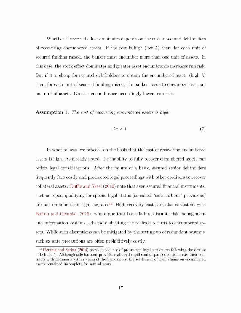
Assumption 1. The cost of recovering encumbered assets is high:

λz < 1. (7)

In what follows, we proceed on the basis that the cost of recovering encumbered

assets is high. As already noted, the inability to fully recover encumbered assets can

reflect legal considerations. After the failure of a bank, secured senior debtholders

frequently face costly and protracted legal proceedings with other creditors to recover

collateral assets. Duffie and Skeel (2012) note that even secured financial instruments,

such as repos, qualifying for special legal status (so-called “safe harbour” provisions)

are not immune from legal logjams.13 High recovery costs are also consistent with

Bolton and Oehmke (2016), who argue that bank failure disrupts risk management

and information systems, adversely affecting the realized returns to encumbered as-

sets. While such disruptions can be mitigated by the setting up of redundant systems,

such ex ante precautions are often prohibitively costly.

13Fleming and Sarkar (2014) provide evidence of protracted legal settlement following the demiseof Lehman’s. Although safe harbour provisions allowed retail counterparties to terminate their con-tracts with Lehman’s within weeks of the bankruptcy, the settlement of their claims on encumberedassets remained incomplete for several years.

17

3.3 Optimal asset encumbrance and secured debt issuance

The banker chooses a ratio of asset encumbrance to maximize the expected value

of bank equity, taking as given the face value of unsecured debt DU , and subject

to the run threshold, A = A∗(α), and the (maximum) amount of secured debt that

can be raised, S ≤ S∗(α). Since a higher level of secured debt for a given ratio of

asset encumbrance both increases the expected equity value of the bank and lowers

fragility, we obtain S = S∗(α). The banker’s problem reduces to

maxα

π ≡∫E2(A)dF (A) =

∫ A∗(α) [RI∗(α)− UDU − S∗(α) r − A

]dF (A). (8)

Figure 3 shows the relationship between encumbrance and expected equity

value.14 A unique interior solution of asset encumbrance exists that balances the

effects of asset encumbrance on the amount of secured debt raised and bank fragility.

α*(��)

��

��

Figure 3: A unique interior privately optimal encumbrance ratio.

14For this and subsequent figures, we use the numerical example of R = 1.5, r = 1.1, E = 0.5,ψ = 0.6, λ = 0.66, γ = 0.8, DU = 3.3 (unless endogenous), and the balance sheet shock follows aGaussian distribution with mean −3 and unit variance.

18

Proposition 2. Asset encumbrance schedule. There is a unique asset encum-

brance schedule, α∗(DU). If fund managers are sufficiently conservative, γ > ψ, then

the schedule decreases in the face value of unsecured debt, dα∗

dDU≤ 0, and an interior

solution for DU < DU < DU is implicitly given by:

F (A∗(α∗))

f(A∗(α∗))=

(1− λz)

λ (z − 1)

[RI∗(α∗)α∗(1− λ) + UDU

(γ

ψ− 1

)]. (9)


The banker balances the marginal benefits and costs of asset encumbrance when

choosing the privately optimal encumbrance ratio. The marginal benefit of encum-

brance is an increase in the amount of secured funding obtained. Since secured debt

is cheap and investments are profitable, the equity value of the bank – conditional on

surviving an unsecured debt run – is higher. But the marginal cost of encumbrance

is an increase in bank fragility and, therefore, a lower probability of surviving an

unsecured debt run. So a higher face value of unsecured debt exacerbates rollover

risk and lowers the run threshold, inducing the banker to encumber fewer assets.

3.4 Pricing of unsecured debt

The repayment of unsecured debt depends on the size of the balance sheet shock. In

the absence of a run, A ≤ A∗, unsecured debtholders receive the promised payment

DU , while for larger shocks, A > A∗, bankruptcy occurs and they receive zero. The

value of an unsecured debt claim is V (DU , α) ≡ DU F (A∗(α,DU)) and competitive

pricing implies that it equals the cost of funding for any given encumbrance ratio:

r = D∗U F (A∗(α,D∗U)). (10)

19

Proposition 3. Private optimum. If bank capital is scarce, E < E, and managers

are conservative, γ ≥ γ˜, then there exists a unique face value of unsecured debt, D∗U >

r. If funding is costly, r > r˜, asset encumbrance is interior, α∗∗ ≡ α∗(D∗U) ∈ (0, 1).


Figure 4 shows the privately optimal allocation and its construction. The condi-

tion γ ≥ γ˜ ensures that the schedule D∗U(α), which is derived from the market clearing

condition for the face value of unsecured debt, is upward-sloping in the vicinity of

the asset encumbrance schedule. This, in turn, leads to a unique characterization of

the joint equilibrium for the ratio of asset encumbrance, α∗∗, and the face value of

unsecured debt, D∗∗U . Next, the condition that the bank’s capital must satisfy E < E

ensures that D∗U < DU(α∗), and that the illiquidity condition is more binding that the

insolvency condition for the bank, as supposed. Finally, the lower bound on the cost

of funding ensures that the equilibrium face value of unsecured debt is sufficiently

high, such that the equilibrium ratio of asset encumbrance is interior.

α*(��)

��* (α)

��(α

*)

��**

α**

��

��

Figure 4: Privately optimum of asset encumbrance and face value of unsecured debt.

20

4 Testable implications

Our model yields a rich set of comparative static results. Parameter changes affect

the unique interior equilibrium in two ways. First, for a given face value of unsecured

debt, the banker trades off heightened fragility against more profitable investment

funded with cheap secured debt. Second, the equilibrium face value of unsecured

debt changes with underlying parameter values, influencing the required face value

for investors to hold unsecured debt. We summarize the main results in Proposition

4, before discussing each of them in turn.

Proposition 4. The banker’s privately optimal ratio of asset encumbrance, α∗∗, de-

creases in the cost of funding, r, conservatism of fund managers, γ, and the costs

of recovering encumbered assets, 1 − λ. Encumbrance increases in the profitability

of investment, R, improvements in the shock distribution F (·), and the liquidation

value, ψ. Greater bank capital, E, has an ambiguous effect on asset encumbrance.


Profitability and risk. Higher returns on investment or a more favorable distri-

bution of the balance sheet shock – in the sense of a first-order stochastic dominance

shift according to the reverse hazard rate – reduces fragility and induces the banker

to encumber more. Therefore, the model implies that banks with less risky balance

sheets or more profitable assets increase the share of secured debt on their balance

sheet. Consistent with these implications, DiFilippo et al. (2016) and Banal-Estanol

et al. (2017) document that banks with higher risks reduce their share of secured debt

and asset encumbrance, respectively.

21

Monetary policy. A lower cost of funding, perhaps brought about by easier mon-

etary conditions, increases secured debt issuance and increases the benefits of asset

encumbrance. Since the required face value of unsecured debt is also lowered, the two

effects combine to increase asset encumbrance, dα∗∗

dr< 0.

Our model suggests that less restrictive monetary conditions lead to a shift to-

ward secured lending. This implication appears consistent with the stylized evidence

in the wake of the global financial crisis. Since 2007/8, central banks in advanced

countries have run expansionary monetary policy and there has been an increased ap-

petite for safe assets among investors (IMF, 2013; Caballero et al., 2016). Consistent

with this implication, Juks (2012) and Bank of England (2012) document a clear,

increasing trend in the encumbrance ratios of Swedish and UK banks following the

implementation of extraordinary monetary policy measures in response to the crisis.

Liquidation values. Higher liquidation values decrease the degree of strategic com-

plementarity among fund managers for a given ratio of asset encumbrance, reducing

illiquidity and fragility at t = 1. Hence, the banker encumbers more assets and

increases profitable investment. Lower fragility, in turn, reduces the face value of un-

secured debt required for investors to participate, increasing encumbrance further.15

Recovery costs. A decrease in the cost of recovering encumbered assets has two

effects. First, for each unit of secured funding, the banker has to encumber fewer

assets. So for a given ratio of asset encumbrance, the banker can raise more secured

funding. Second, there are more unencumbered assets available to meet withdrawals

at t = 1, which reduces fragility. This, in turn, lowers the face value of unsecured

debt. Taking both effects into account, there is greater asset encumbrance, dα∗∗

dλ> 0.

15Chen et al. (2010) show that illiquid mutual funds face greater redemptions than liquid funds.

22

Market stress. The conservatism parameter γ can be broadly interpreted as a

measure of market stress. Krishnamurthy (2010) documents how, during the global

financial crisis, fund managers turned conservative and became less inclined to roll

over unsecured debt. Faced with a deterioration in investor sentiment, the bank is

more fragile for a given encumbrance ratio. The banker responds to the heightened

fragility in a precautionary fashion, lowering the extent of encumbrance and forgoing

profitable investment from the issuance of secured debt in order to induce rollovers

by fund managers. The combined effects of increased fragility and the greater face

value of unsecured debt reduce encumbrance, so dα∗∗

dγ< 0. Increased market stress

thus induces a reduction in the share of secured debt (as a proportion of total debt).

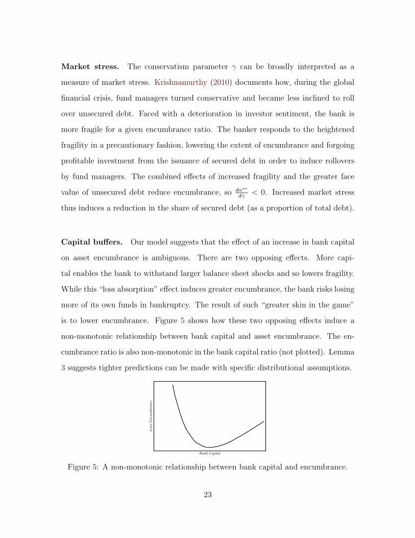
Capital buffers. Our model suggests that the effect of an increase in bank capital

on asset encumbrance is ambiguous. There are two opposing effects. More capi-

tal enables the bank to withstand larger balance sheet shocks and so lowers fragility.

While this “loss absorption” effect induces greater encumbrance, the bank risks losing

more of its own funds in bankruptcy. The result of such “greater skin in the game”

is to lower encumbrance. Figure 5 shows how these two opposing effects induce a

non-monotonic relationship between bank capital and asset encumbrance. The en-

cumbrance ratio is also non-monotonic in the bank capital ratio (not plotted). Lemma

3 suggests tighter predictions can be made with specific distributional assumptions.

��

��

Figure 5: A non-monotonic relationship between bank capital and encumbrance.

23

Lemma 3. If the balance sheet shock is uniformly distributed, then the privately

optimal ratio of asset encumbrance monotonically increases in bank capital.


5 Policy implications

In many countries, unsecured debtholders often enjoy the benefits of explicit (or im-

plicit) government guarantees. These schemes, which typically apply to retail depos-

itors, often extend to wholesale depositors during times of crisis. Although deposit

insurance and wholesale funding guarantee schemes have been studied previously,

their relationship with asset encumbrance has yet to be examined.16 Specifically,

while guarantee schemes aim to reduce bank fragility ex post, their presence distorts

behavior ex ante. By externalizing the costs of the guarantee upon failure, the banker

has incentives to excessively encumber assets that, in turn, creates excessive fragility.

Our model provides a natural framework for the normative analysis of this

issue. Let a fraction 0 < m < 1 of unsecured debt be fully and credibly guaranteed.17

Since guaranteed debt is safe, it is never subject to a run. Let the face value of

guaranteed unsecured debt be DG. If the fraction ` of unsecured non-guaranteed

debt is withdrawn, then the bank is illiquid at t = 1 whenever

R(1− α)I − A ≤ `(1−m)UDU

ψ, (11)

where the guarantee reduces the illiquidity of the banker at t = 1 for given funding

16Earlier contributions include Kareken and Wallace (1978); Diamond and Dybvig (1983);Calomiris (1990); Matutes and Vives (1996), and Cooper and Ross (2002).

17In the spirit of Allen et al. (2015), we consider guarantees that eliminate both inefficient andefficient runs. As the authors argue, such a guarantee scheme resembles real-world deposit insurance.

24

choices. Similarly, the bank is insolvent at t = 2 whenever

RI − A− `(1−m)UDU

ψ≤ SDS + (1− `)(1−m)UDU +mUDG, (12)

where the guarantee reduces the insolvency of the banker at t = 2, since guaranteed

unsecured debt is not subject to rollover risk at t = 1 and cheaper in any equilibrium.

The equilibrium in secured debt and guaranteed unsecured debt is as follows.

Since guaranteed debt is safe, we have D∗G = r, in any equilibrium. The balance sheet

shock has full support, so the bank is closed early at t = 1 with positive probability

for any given guarantee coverage. Moreover, since the guarantee has no bearing on

how encumbered assets are managed following early closure, Lemma 1 continues to

hold, implying D∗S = r and S∗ = S∗(α) and I∗ = I∗(α).18

Figure 6 shows how introducing the guarantee affects run dynamics. The illiq-

uidity and insolvency thresholds, respectively, depend on the volume of withdrawals:

AIL(`) = R(1− α)I∗(α)− `(1−m)UDU

ψ, (14)

AIS(`) = R(1− αλ)I∗(α)− UDU(1−m)

(1 + `

[1

ψ− 1

]). (15)

Guarantees reduces the responsiveness of both thresholds to changes in the withdrawal

volume. As before, the illiquidity threshold is still more sensitive to withdrawals than

the insolvency threshold. Moreover, the insolvency threshold shifts outwards, while

18The upper bound on the face value of unsecured debt is more relaxed with guarantees. Thus,the conditions previously imposed continue to suffice for the illiquidity threshold to be more bindingthan the insolvency threshold, irrespective of guarantee coverage. To see this, the bound is

DU ≤ DU (m) ≡ 1

1−m

[Rα(1− λ)I∗(α)

U−mr

]. (13)

A higher coverage of the guarantee relaxes the condition in equation (13), since ∂DU (m)/∂m =(DU (m)− r)/(1−m) ≥ 0 because DU ≥ r in any equilibrium.

25

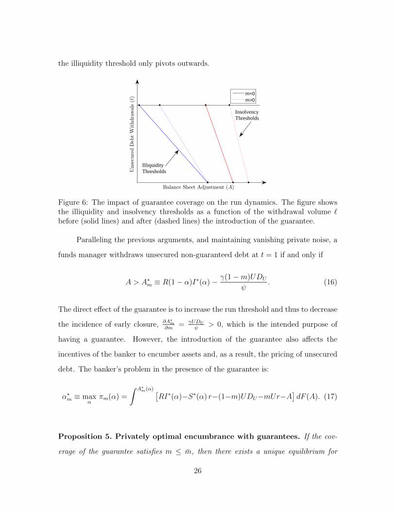
the illiquidity threshold only pivots outwards.


UnsecuredDebtW

ithdrawals(�)

IlliquidityThresholds

InsolvencyThresholds

m=0m>0

Figure 6: The impact of guarantee coverage on the run dynamics. The figure showsthe illiquidity and insolvency thresholds as a function of the withdrawal volume `before (solid lines) and after (dashed lines) the introduction of the guarantee.

Paralleling the previous arguments, and maintaining vanishing private noise, a

funds manager withdraws unsecured non-guaranteed debt at t = 1 if and only if

A > A∗m ≡ R(1− α)I∗(α)− γ(1−m)UDU

ψ. (16)

The direct effect of the guarantee is to increase the run threshold and thus to decrease

the incidence of early closure, ∂A∗m

∂m= γUDU

ψ> 0, which is the intended purpose of

having a guarantee. However, the introduction of the guarantee also affects the

incentives of the banker to encumber assets and, as a result, the pricing of unsecured

debt. The banker’s problem in the presence of the guarantee is:

α∗m ≡ maxα

πm(α) =

∫ A∗m(α) [

RI∗(α)−S∗(α) r−(1−m)UDU−mUr−A]dF (A). (17)

Proposition 5. Privately optimal encumbrance with guarantees. If the cov-

erage of the guarantee satisfies m ≤ m, then there exists a unique equilibrium for

26

the ratio of asset encumbrance and face value of unsecured debt. The presence of

guarantees increases the ratio of asset encumbrance, α∗∗m > α∗∗.


The presence of a guarantee has two intuitive effects. First, the stock of unse-

cured debt that may be withdrawn at t = 1 is reduced, which lowers the incidence

of runs. As a result, the banker has more incentives to encumber assets, which shifts

the encumbrance schedule α∗m(DU) outward. Second, unsecured debt without a guar-

antee is repaid with greater probability, since the run threshold increases. This, in

turn, reduces the face value of unsecured debt and shifts the participation constraint

of investors D∗U(α) inward. In sum, the introduction of the guarantee unambiguously

increases the encumbrance ratio, α∗∗m , but has an ambiguous effect on the equilibrium

face value of unsecured debt, D∗∗m ≡ D∗U(α∗∗m ).

The banker ignores the social cost of providing the guarantee, so the guarantee

distorts the banker’s incentives to encumber assets.19 In contrast, a planner accounts

for these costs, mUr, which are incurred when the bank fails. The ex-ante probability

of bank failure is 1−F (A∗m). We assume that the planner takes as given the incomplete

information structure (that is, the private information of fund managers about balance

sheet adjustment) and the face value of unsecured non-guaranteed debt. Thus, the

planner’s asset encumbrance schedule for a given face value of unsecured debt is:20

19As stated in the introduction, we abstract from explicitly modeling premiums for deposit in-surance (DI). Since these premiums are typically insensitive to encumbrance ratios, a bank still hasan incentive to encumber assets excessively even if premiums are otherwise fairly priced. See alsoProposition 7 and our interpretation of the tax as an encumbrance surcharge to the DI premium.

20In our analysis, we abstracts from the payoffs to fund managers. Using the payoffs proposed byRochet and Vives (2004), these are bF (A∗) in equilibrium. Because of vanishing private noise, eachfund manager refuses to roll over unsecured debt exactly when the bank fails at t = 1. Accounting forthese payoffs, however, would increase the gap between the privately and socially optimal ratios ofencumbrance, since the probability of bank survival is lower under excessive encumbrance. Therefore,our results on the welfare-enhancing effect of regulation are reinforced.

27

α∗P (DU) ≡ maxα

πm(α)−[1− F (A∗m(α))

]mUr. (18)

While the asset encumbrance schedules of the banker and planner differ, the par-

ticipation constraint of unsecured debtholders is the same and given by the same

participation constraint schedule for investors, D∗U(α). So any difference in alloca-

tions is due to differences in the respective asset encumbrance schedules. The face

value of unsecured debt chosen by the planner, denoted by D∗∗P , solves the fixed point

problem D∗∗P ≡ D∗U(α∗P (D∗U)). Figure 7 shows the asset encumbrance schedules and

the pricing of unsecured non-guaranteed debt, as well as the privately and socially

optimal ratios of asset encumbrance and face values of debt.

Proposition 6. Excessive encumbrance. The privately optimal levels of asset

encumbrance and the face value of unsecured non-guaranteed debt are excessive, α∗∗m >

α∗∗P and D∗∗m > D∗∗P , respectively.


Prudential safeguards. We now consider several policy tools to curb excessive

encumbrance and fragility in the presence of guarantees. In particular, we consider a

limit to asset encumbrance, α ≤ α as an additional constraint to the banker’s problem.

We consider policies that are less information-intensive for the policymaker, notably

lump-sum taxes and transfers, T , and linear, revenue-neutral Pigovian taxes on asset

encumbrance. Let α∗R(DU) denote the banker’s optimal asset encumbrance schedule

subject to some regulation.

28

α�* (��)

α�* (��)

��

*(α)

��** ��

**

α�**

α�**

��

��

Figure 7: Excessive encumbrance and fragility with a guarantee scheme: the sociallyoptimal asset encumbrance schedule lies below the privately optimal schedule forany given face value of debt, α∗P (DU) ≤ α∗m(DU). Since the competitive pricing ofunsecured and non-guaranteed debt is the same for the planner and the banker, theprivately optimal ratios of asset encumbrance and face value of debt are excessive.

Proposition 7. Optimal regulation. In the presence of the guarantee, m > 0, a

planner achieves the social optimum (α∗∗P , D∗∗P ) by imposing:

a. a limit on asset encumbrance at α∗∗P ;

b. a transfer T = Umr to the banker at t = 2;

c. a contingent linear tax on asset encumbrance imposed at t = 2, combined with

a lump-sum rebate of the generated revenue, T = ατ . The optimal rate is

τ ∗(DU) =(1− λz)RI∗(α∗P )Umrf(A∗m(α∗P ))

(1− λzα∗P )F (A∗m(α∗P )), (19)

which depends on the face value of unsecured non-guaranteed debt.

d. a linear tax on asset encumbrance at t = 2 that is not contingent on the face

value of debt, combined with a lump-sum rebate of the generated revenue. That

is, there exists a unique rate τ ∗ > 0 such that α∗∗R (τ ∗) = α∗∗P and D∗∗R (τ ∗) = D∗∗P .


29

Figure 8 shows the impact of a limit on asset encumbrance. When the constraint

α ≤ α∗∗P is added to the banker’s problem, the banker’s constrained encumbrance

schedule for any given face value of debt is

α∗R(DU) ≡

α∗m(DU) α∗m(DU) < α∗∗P

if

α∗∗P α∗m(DU) ≥ α∗∗P .

(20)

The banker chooses the socially optimal encumbrance ratio and, therefore, un-

secured debt is also priced at the socially optimal level. In sum, when the planner

directly controls encumbrance at t = 0, a limit on encumbrance is effective.

The encumbrance cap can also be implemented via bank capital regulation.

The bank’s capital ratio at t = 0 (inverse leverage ratio), e ≡ e(α) = E0

I∗(α), is

sensitive to changes in the encumbrance ratio, specifically dedα< 0. Thus, a minimum

capital ratio, e ≥ e, translates into a bound on asset encumbrance in our model.

Thus, the social optimum can be achieved by requiring that the bank’s capital ratio

satisfies e > e(α∗∗P ). This argument generalizes to risk-based capital requirements if

encumbered and unencumbered assets carry different risk-weights.

α�* (��)

α�* (��)

��

*(α)

��**

α�**

��

��

Figure 8: A limit on asset encumbrance avoids excessive encumbrance and fragility.

30

We proceed to consider tools that do not require the planner to observe the

encumbrance ratio at t = 0. Figure 9 shows how a transfer to the banker at t = 2

achieves the social optimum. When the banker receives the market value of non-

guaranteed unsecured debt, Umr, it internalizes the effect of its failure on the cost of

providing the guarantee. A benefit of this transfer is that the planner does not need

to observe the encumbrance ratio at all. However, the size of this transfer may be

large and its implementation, therefore, subject to political constraints.

α�* (��)

α�* (��)

��

*(α)

��** ��

**

α�**

α�**

��

��

Figure 9: A transfer of the market value of guaranteed unsecured debt aligns thesocially and privately optimal asset encumbrance schedules. Such a transfer inducesthe banker to internalize the social cost of its failure.

We next turn to revenue-neutral regulation. Specifically, we consider a linear

tax τ on asset encumbrance imposed at t = 2, combined with a lump-sum rebate of

T = τα. A higher tax rate reduces the privately optimal encumbrance of assets, since

the banker’s equity value contingent upon no early closure decreases in encumbrance.

When the tax rate can be contingent on the face value of unsecured non-guaranteed

debt, the optimal rate τ ∗(DU) ensures that the privately and socially optimal asset

encumbrance schedules are aligned for any face value of unsecured debt. This situation

parallels that of a transfer in Figure 9. As a result, the social optimum is attained.

When the tax rate cannot be made contingent on the face value of debt, the

privately and socially optimal encumbrance schedules do not always align, as shown

31

in Figure 10. However, a higher tax rate reduces asset encumbrance, so there exists

a unique rate at which the socially optimum is achieved. Graphically, the privately

optimal asset encumbrance schedule must be shifted inward following the marginal

tax on encumbrance so as to intersect with the social optimum.

α�* (��)

α�* (��)

��

*(α)

��**

α�**

��

��

Figure 10: A non-contingent linear tax on encumbrance with lump-sum rebateachieves the social optimum.

In our analysis, the linear Pigovian tax and its lump-sum rebate are imposed at

t = 2. Since this requires the planner to only observe asset encumbrance at this date,

it can be viewed as a less information-intensive policy tool. The timing assumption

is without loss of generality, however. If a tax and lump-sum rebate scheme were

imposed at t = 1, the banker would internalize the effect of asset encumbrance on

heightened illiquidity and thus a greater incidence of early closure, which induces

the banker to encumber fewer assets.21 If a tax and lump-sum rebate scheme were

imposed at t = 0, the available resources for investment would be affected. The banker

would internalize the effect of great encumbrance on reduced profitable investment,

which also exacerbates illiquidity at t = 1. In sum, a full rebate of the tax revenue

generated ensures that investment at t = 0, the illiquidity condition at t = 1, and

equity value at t = 2 remain unchanged, while aligning the banker’s incentives.

21The credibility of a regulatory measure perceived to heighten fragility at t = 1, precisely whena bank may become illiquid, is a matter of debate, however.

32

Relation to policy debate. The problem of excessive asset encumbrance by banks

has become a growing focus of attention for policymakers. Banks have increasingly

turned to secured funding in a quest for safety that may, ultimately, be counterpro-

ductive. Policymakers have expressed concern that the increased collateralization of

bank balance sheets can heighten rollover risk and, hence, bank fragility, as well as

increase the procylicality of the financial system (Haldane, 2012; CGFS, 2013).

The prudential safeguards considered in this section speak to some of these con-

cerns. Policymakers in some countries are seeking to address excessive encumbrance

by imposing explicit restrictions on the share of bank assets that can be encumbered.

These restrictions apply either (a) through limits on assets that can be pledged when

secured debt is issued; or (b) via limits on bond issuance. In the context of our model,

these asset and liability side restrictions are equivalent and map directly into the cap

on asset encumbrance. Table 4 summarizes the restrictions implemented.

Country Policies

Assets Liabilities

Australia 8%

Belgium 8%

Canada 4%

Greece 20%

Italy

25% of assets if 6% ≤ CET1 < 7%

60% of assets if 7% ≤ CET1 < 8%

No Limit if CET1 ≥ 8%

NetherlandsDetermined on a case-by-case basis, such that the ratioof encumbered to total assets must be a ‘healthy ratio’

New Zealand 10%

United States 4%

Table 4: Caps on asset encumbrance across different countries

33

While most countries have adopted a cap on encumbered assets, the United

States has implemented a policy to cap the share of secured debt to total liabilities.

In Italy, the asset encumbrance cap is contingent on a bank’s Core Equity Tier 1

capital ratio (CET1). However, as we have shown, there is a non-linear relationship

between asset encumbrance and bank capital (and also capital ratio). So the effects

of such a policy for fragility may not be clear-cut.

In our model, the cap on asset encumbrance is set at the level that maximizes

the social planner’s objective function. But the cap can, in practice, be sensitive

to broader economic and financial conditions. So, to maintain a socially desirable

outcome, policymakers may need to consider asset encumbrance policies that vary

over time. In the Netherlands, for example, the cap is set on a case-by-case basis

for individual banks, taking into account the financial position, solvency risk of the

issuing bank, its risk profile and the riskiness inherent in its assets (see DNB, 2015).

A form of Pigovian taxation to address the externalities posed by asset encum-

brance has also been implemented in Canada. The deposit insurance premiums levied

by the Canadian Deposit Insurance Corporation (CDIC, 2017) on systemically impor-

tant domestic banks reflects the extent to which their balance sheet is encumbered.

Specifically, 5% of the score used to calculate the deposit insurance premium paid

by these banks reflects asset encumbrance considerations. Such a surcharge can be

viewed as being similar in spirit to the asset encumbrance tax analyzed above, al-

though the extent to which the CDIC surcharge is revenue-neutral is open to debate.

34

6 Additional Implications

We conclude the analysis by considering the implications of (i) a risk premium between

risk-neutral and risk-averse investors; (ii) a limited wealth constraint for risk-averse

investors; and (iii) the precision of private information about the balance sheet shock.

6.1 Risk premium on unsecured debt

The required return for risk-averse and risk-neutral investors has been the same so

far. We now suppose that risk-neutral investors require a risk premium. Formally,

investors have access to a menu of risk-free and risky storage. The return on risk-free

storage continues to be r but the expected return on risky storage is r > r, implying

a risk premium of p ≡ r − r. We derive an additional testable implication about the

risk premium. The risk premium does not affect the pricing of secured debt and the

illiquidity condition, so D∗S = r, S∗(α), and A∗(α) are unchanged. Since the banker

takes the face value of unsecured debt as given, the privately optimal encumbrance

ratio, α∗(DU), is also unchanged. But the pricing of unsecured debt is affected, as

the competitive pricing schedule D∗U(α; p) shifts out as the premium increases.

α*(��)��* (α)

��

*(α)

��**

��**

α**

α**

��

��

Figure 11: A higher risk premium reduces asset encumbrance and increases the facevalue of unsecured debt.

35

Proposition 8. A higher risk premium, p, decreases the privately optimal ratio of

asset encumbrance, α∗∗, and increases the face value of unsecured debt, D∗∗U .

6.2 Limited wealth

In our model, the banker trades off more profitable investment, funded by cheap

secured debt, against greater fragility when choosing asset encumbrance. This mech-

anism relies on the pool of risk-averse investors being sufficiently large, such that the

banker can obtain secured funding up to the level where the marginal benefit from

an additional unit of cheap funding is equal to the marginal cost of greater fragility.

This trade-off, however, can break down once the wealth of risk-averse investors is

limited. In what follows, we investigate this case formally.

Suppose that a mass ω of risk-averse investors has a unit endowment. So the

supply of funds by risk-averse investors, given by their binding participation con-

straint, is:

D∗S ≡

r α ≤ α ≡ ω

λz(U+E+ω)

if

r λz(U+E+ω)ω

α α > α,

(21)

where α is the proportion of total investment at which the total wealth of risk-averse

investors is attracted with secured debt. The amount of secured debt raised is:

S∗(α) ≡

αλzI∗(α) α ≤ α

if

ω α > α.

(22)

36

As before, the cost of greater asset encumbrance is greater fragility, whereby

dA∗

dα< 0. However, there is no longer a benefit of greater asset encumbrance when

the wealth of risk-averse investors is scarce, since no additional secured debt can be

issued. Moreover, the equilibrium face value of secured debt increases in asset encum-

brance, further reducing the expected equity value of the banker as asset encumbrance

increases. Therefore, it is never optimal to encumber more assets than α.

6.3 Limited precision of information and liquidity support

In the limit of infinitely precise private information about the balance sheet shock, ε→

0, the mass of fund managers who withdraw is a step function, `∗(A, x) = 1{A>A∗}. If

the bank’s insolvency and illiquidity lines are sufficiently close, then `∗(A, x) crosses

both curves for the same threshold level A∗, implying that the illiquidity and insol-

vency thresholds are the same. For finite precision, by contrast, the mass of fund

managers who withdraw is `∗(A, x∗) = H(x∗ − A), which is a sigmoidal function.

Consequently, the illiquidity and insolvency thresholds differ (Figure 12).

ℓ*(�)

��(ℓ)

��(ℓ)

�*

�� (�)

��(ℓ)

ℓ*(�)

��(ℓ)

��(ℓ)

��* ��

*

γ

�� (�)

��(ℓ)

Figure 12: The precision of private information and the range of balance sheet shocksfor which a bank is illiquid but solvent. The top panel shows the case of infinitelyprecise private information and DU ≥ ψ

1−γ DU , so A∗∗IL = A∗∗IS. The bottom panel

shows the case of limited precision of private information and the range [A∗∗IL, A∗∗IS].

37

For values of the balance sheet shock in the wedge between the illiquidity and

insolvency thresholds, the bank is indeed illiquid but solvent. This opens up a role

for a lender of last-resort, as considered by Rochet and Vives (2004). In particular,

if the central bank observes the shock without noise – perhaps due to its supervisory

function – it can offer loans at an interest rate ρ ∈ [0, 1ψ− 1). Such a lender of

last resort policy shifts out the illiquidity threshold for any given encumbrance ratio.

Since the bank is truly solvent, no taxpayer’s money is at risk. An alternative support

mechanism is costly liquidity injections (Cong et al., 2017). In the context of our

model, such an intervention shifts up the illiquidity threshold by an amount φ at

an exogenous cost k(φ). With credible commitment, such a policy balances the cost

with the endogenous benefit of reducing both fragility and the cost of unsecured debt.

Both forms of liquidity support affect the banker’s incentives to encumber assets at

t = 0. Detailed consideration of this issue is, however, left for future research.

7 Conclusion

Banks increasingly rely on secured funding attracted by encumbering assets: a bank

ring-fences and legally separates some assets on its balance sheet into a bankruptcy-

remote vehicle. In this paper, we offer a model of asset encumbrance by banks subject

to rollover risk and examine its effect on the fragility and funding costs of banks.

The privately optimal encumbrance ratio trades off expanding profitable investment

funded by cheap secured debt with greater fragility due to unsecured debt runs. We

derive and discuss several testable implications about the encumbrance ratios and

secured funding shares of banks. Deposit insurance and wholesale funding guaran-

tees induce excessive encumbrance and exacerbates fragility. To mitigate these risk-

shifting incentives, we show how prudential regulation of banks should be designed.

38

References

Allen, F., E. Carletti, I. Goldstein, and A. Leonello (2015). Government guarantees and

financial stability. CEPR Discussion Paper 10560.

Auh, J. and S. Sundaresan (2015). Repo rollover risk and the bankruptcy code. Mimeo,

Columbia Business School.

Ayotte, K. and S. Gaon (2011). Asset-Backed Securities: Costs and Benefits of “Bankruptcy

Remoteness”. Review of Financial Studies 24, 1299–1336.

Banal-Estanol, A., E. Benito, and D. Khametshin (2017). Asset encumbrance and bank

risk: First evidence from public disclosures in Europe. CEPR Discussion Paper 12168.

Bank of England (2012). Three medium-term risks to financial stability. Financial Stability

Report 31, 30–46.

Bolton, P. and M. Oehmke (2016). Bank resolution and the structure of global banks.

Mimeo, Columbia Business School.

Caballero, R., E. Farhi, and P.-O. Gourinchas (2016). Safe asset scarcity and aggregate

demand. American Economic Review 106 (5), 513–18.

Calomiris, C. (1990). Is deposit insurance necessary? A historical perspective. The Journal

of Economic History 50, 283–95.

Calomiris, C. and C. Kahn (1991). The Role of Demandable Debt in Structuring Optimal

Banking Arrangements. American Economic Review 81 (3), 497–513.

Carlsson, H. and E. van Damme (1993). Global games and equilibrium selection. Econo-

metrica 61 (5), 989–1018.

CDIC (2017). Differential premiums by-law manual. http://www.cdic.ca/en/financial-

community/Pages/differential-premiums.aspx .

39

CGFS (2013). Asset encumbrance, financial reform and the demand for collateral assets.

Committee on the Global Financial System Publications No. 49, BIS, Basel .

Chen, Q., I. Goldstein, and W. Jiang (2010). Payoff complementarities and financial

fragility: Evidence from mutual fund outflows. Journal of Financial Economics 97 (2),

239–62.

Cong, L., S. Grenadier, and Y. Hu (2017). Intervention policy in a dynamic environment:

Coordination and learning. Mimeo, University of Chicago Booth School of Business.

Cooper, R. and T. Ross (2002). Bank runs: Deposit insurance and capital requirements.

International Economic Review 43 (55–72).

Diamond, D. and P. Dybvig (1983). Bank runs, deposit insurance and liquidity. Journal of

Political Economy 91, 401–419.

Diamond, D. and R. Rajan (2001). Liquidity risk, liquidity creation, and financial fragility:

A theory of banking. Journal of Political Economy 109 (2), 287–327.

DiFilippo, M., A. Ranaldo, and J. Wrampelmeyer (2016). Unsecured and secured funding.

Mimeo, University of St. Gallen.

DNB (2015). Testing of a healthy ratio of covered bonds to disposable assets. http:

//www.toezicht.dnb.nl/en/3/51-203144.jsp.

Duffie, D. and D. Skeel (2012). Bankruptcy Not Bailout: A Special Chapter 14, Chapter A

Dialogue on the Costs and Benefits of Automatic Stays for Derivatives and Repurchase

Agreements. Hoover Press.

EBA (2016). European Banking Authority Report on Asset Encumbrance.

ECB (2016). Recent developments in the composition and cost of bank funding in the euro

area. Economic Bulletin, 26–42.

40

http://www.toezicht.dnb.nl/en/3/51-203144.jsp

http://www.toezicht.dnb.nl/en/3/51-203144.jsp

Eisenbach, T. (2017). Rollover risk as market discipline: A two-sided inefficiency. Journal

of Financial Economics Forthcoming.

Eisenbach, T., T. Keister, J. McAndrews, and T. Yorulmazer (2014). Stability of funding

models: an analytical framework. FRBNY Economic Policy Review .

Fleming, M. and A. Sarkar (2014). The failure resolution of Lehman Brothers. Federal

Reserve Bank of New York Economic Policy Review 20, 175–206.

Frankel, D., S. Morris, and A. Pauzner (2003). Equilibrium selection in global games with

strategic complementarities. Journal of Economic Theory 108 (1), 1–44.

Gai, P., A. Haldane, S. Kapadia, and B. Nelson (2013). Bank funding and financial sta-

bility. In A. Heath, M. Lilley, and M. Manning (Eds.), Liquidity and Funding Markets:

Proceedings of the Reserve Bank of Australia Annual Conference, pp. 237–52.

Goldstein, I. and A. Pauzner (2005). Demand deposit contracts and the probability of bank

runs. Journal of Finance 60 (3), 1293–1327.

Haldane, A. (2012). Financial arms races. Speech at the Institute for New Economic Think-

ing, April 14, Centre for International Governance Innovation and Mercator Research

Institute on Global Commons and Climate Change Third Annual Plenary Conference

‘Paradigm Lost: Rethinking Economics and Politics’, Berlin.

Hardy, D. (2014). Bank resolution costs, depositor preference and asset encumbrance.

Journal of Financial Regulation and Compliance 22, 96–114.

Helberg, S. and S. Lindset (2014). How do asset encumbrance and debt regulations affect

bank capital and bond risk? Journal of Banking and Finance 44, 39–54.

IMF (2012). Chapter III: Safe Assets – Financial System Cornerstone? Global Financial

Stability Report , 3547–92.

IMF (2013). Global Financial Stability Report, April.

41

Juks, R. (2012). Asset encumbrance and its relevance for financial stability. Sveriges

Riksbank Economic Review 3, 67–89.

Kareken, J. and N. Wallace (1978). Deposit insurance and bank regulation: A partial-

equilibrium exposition. The Journal of Business 51, 413–438.

Krishnamurthy, A. (2010). How debt markets have malfunctioned in the crisis. Journal of

Economic Perspectives 24, 3–28.

Matta, R. and E. Perotti (2017). Insecure debt and liquidity runs. Mimeo, University of

Amsterdam.

Matutes, C. and X. Vives (1996). Competition for deposits, fragility, and insurance. Journal

of Financial Intermediation 5, 184–216.

Morris, S. and H. Shin (2001). NBER Macroeconomics Annual 2000, Volume 15, Chapter

Rethinking Multiple Equilibria in Macroeconomic Modeling, pp. 139–182. MIT Press.

Morris, S. and H. Shin (2003). Global games: Theory and Applications. In M. Dewatripont,

L. Hansen, and S. Turnovsky (Eds.), Advances in Economics and Econometrics (Proceed-

ings of the 8th World Congress of the Econometric Society). Cambridge University Press.

Ranaldo, A., M. Rupprecht, and J. Wrampelmeyer (2017). Fragility of money markets.

Mimeo, University of St. Gallen.

Rochet, J.-C. and X. Vives (2004). Coordination failures and the Lender of Last Resort: was

Bagehot right after all? Journal of the European Economic Association 2 (6), 1116–47.

Vives, X. (2005). Complementarities and Games: New Developments. Journal of Economic

Literature 43, 437–479.

Vives, X. (2014). Strategic complementarity, fragility, and regulation. Review of Financial

Studies 27 (12), 3547–92.

42

A Proofs

A.1 Proof of Proposition 1

The proof is in three steps. First, we show that the dominance regions at the rollover stage,

based on the illiquidity threshold, are well defined for any bank funding structure. If the

balance sheet shock were common knowledge, the rollover behavior of fund managers would

be characterized by multiple equilibria, as shown in Figure 13. If no unsecured debt is rolled

over, ` = 1, the bank is liquid at t = 1 whenever the shock is below a lower dominance

bound A ≡ R(1 − α)I − UDUψ . For A < A, it is a dominant strategy for fund managers to

roll over. If ` = 0, the bank is illiquid whenever the shock is above an upper dominance

bound A ≡ R(1− α)I. For A > A, it is a dominant strategy for managers not to roll over.

- A

A A

Liquid Liquid / Illiquid Illiquid

Roll over Multiple equilibria Withdraw

Figure 13: Tripartite classification of the balance sheet shock

Second, in any rollover stage, it suffices to establish the optimality of threshold strate-

gies for sufficiently precise private information. Morris and Shin (2003) and Frankel et al.

(2003) show that only threshold strategies survive the iterated deletion of strictly dominated

strategies. Thus, each fund manager i uses a threshold strategy, whereby unsecured debt

is rolled over if and only if the private signal about the balance sheet shock is below some

signal threshold, xi < x∗. We consider vanishing private noise, ε→ 0, in the main text.

Third, we characterize this threshold equilibrium. For a given realization A ∈ [A,A ],

the proportion of fund managers who do not roll over unsecured debt is:

`(A, x∗

)= Prob

(xi > x∗

∣∣A) = Prob (εi > x∗ −A) = 1−H(x∗ −A

). (23)

43

A critical mass condition states that illiquidity occurs when the shock equals A∗, where

the proportion of managers not rolling over is evaluated at A∗:

R(1− α)I −A∗ = `(A∗, x∗

)UDU

ψ. (24)

The posterior distribution of the shock conditional on the private signal is derived using

Bayes’ rule. An indifference condition states that the manager who receives the threshold

signal xi = x∗ is indifferent between rolling and not rolling over, γ = Pr (A < A∗|xi = x∗).

Using the definition xj = A+ εj , the conditional probability is

1− γ = Pr (A ≥ A∗|xi = x∗) = Pr (A ≥ A∗|xi = x∗ = A+ εj) , (25)

= Pr (x∗ − εj ≥ A∗) = Pr (εj ≤ x∗ −A∗) = H(x∗ −A∗

). (26)

The indifference condition implies x∗ − A∗ = H−1(1 − γ

). Inserting this expression into

`(A∗, x∗

), the proportion of managers who do not roll over at the threshold shock level

A∗ is perceived by the indifferent manager to be `(A∗, xi = x∗

)= 1 − H

(x∗ − A∗

)=

1−H(H−1

(1− γ

))= γ. The run threshold A∗ stated in Proposition 1 follows. It varies

with the face value of unsecured debt and asset encumbrance according to:

dA∗

dDU= −γU

ψ< 0,

dA∗

dα= R (λz − 1)

I∗(α)

1− αλz. (27)


The banker’s problem is given in (8). The total derivative dπdα , which takes indirect effects

via A∗(α) and S∗(α) into account, yields dπdα = RI∗(α)

1−αλz f(A∗)G(α), where

G(α) =F (A∗)

f(A∗)λ(z − 1)− (1− λz)

[RI∗(α)α(1− λ) + UDU

(γ

ψ− 1

)]. (28)

If an interior solution 0 < α∗ < 1 exists, it is given by G(α∗) = 0. It is a local maximum:

44

dG

dα=dF (A∗)f(A∗)

dA∗︸︷︷︸+

dA∗

dα︸︷︷︸−

λ(z − 1)− (1− λz)R(1− λ)I∗(α)

1− αλz< 0, (29)

where the first term is positive since f(A) possesses decreasing reverse hazard rate. Using

the implicit function theorem (IFT), we obtain dα∗

dDU< 0 for the interior solution since

dG

dDU=dF (A∗)f(A∗)

dA∗dA∗

dDUλ(z − 1)− (1− λz)U

(γ

ψ− 1

)< 0 (30)

where we used γ > ψ. Hence, the weak inequality dα∗

dDU≤ 0 follows for the entire schedule

of asset encumbrance. We next examine if the solution to G(α∗) = 0 is interior. An interior

solution requires two conditions, G(α = 0) > 0 and G(α = 1) < 0, which we consider in

turn. First, evaluating the implicit function when there is no encumbrance, α = 0, yields

F (A∗(0))

f(A∗(0))λ(z − 1)− (1− λz)

(γ

ψ− 1

)UDU , (31)

which strictly decreases in DU . To ensure α∗ > 0, the face value of unsecured debt must

satisfy DU < DU , where DU is uniquely and implicitly defined by

F (R(U + E)− γψUDU )

f(R(U + E)− γψUDU )

λ(z − 1)− (1− λz)(γ

ψ− 1

)UDU = 0. (32)

Second, evaluating the implicit function when all assets are encumbered, α = 1, yields

F (A∗(1))

f(A∗(1))λ(z − 1)− (1− λz)

[R(1− λ)(U + E)

1− λz+

(γ

ψ− 1

)UDU

], (33)

which also decreases in DU . To ensure α∗ < 1, the expression in equation (33) must be

strictly negative. Hence, the face value of unsecured debt must be bounded from below,

DU > DU , where DU < DU is uniquely and implicitly defined by

F (− γψUDU )

f(− γψUDU )

λ(z − 1)− (1− λz)[R(1− λ)(U + E)

1− λz+

(γ

ψ− 1

)UDU

]= 0 . (34)

45


The proof is in five steps. First, we ensure that the encumbrance ratio is interior, α∗∗ ∈

(0, 1). Since α = 0 implies DU = 0, there is no equilibrium consistent with our supposition

DU ≤ DU , so it must be the case that α∗∗ > 0 (we verify the supposition below). If α = 1,

the run threshold and value of an unsecured debt claim are A∗(1) = −γDUψ and V (1, DU ) =

DUF (A∗(1)), respectively. The value of the unsecured debt claim attains a maximum at

DU = Dmax, which is uniquely and implicitly defined byF(− γψDmax

)f(− γψDmax

) − γψDmax = 0. Since

V (α,DU ) decreases in α, if we impose on the outside option that r > r˜ ≡ V (1, Dmax), then

any solution for the equilibrium ratio of asset encumbrance is interior (if it exists).

Second, we show that the equilibrium face value of unsecured debt satisfies D∗U > r.

To this end, note that while ∂V∂DU

has an ambiguous sign in general, the derivative evaluated

along the asset encumbrance schedule is

∂V

∂DU

∣∣∣∣α∗(DU )

= f(A∗)

[1− λzλ(z − 1)

R(1− λ)α∗I∗(α∗) + β0UDU

], (35)

which is non-negative whenever β0 ≡ 1−λzλ(z−1)

(γψ − 1

)− γ

ψ ≥ 0 ↔ γ ≥ γ˜ ≡ 1−λz1−λz−λ(z−1)ψ.

Having established conditions under which V increases in DU , at least in the vicinity of

the asset encumbrance schedule, it follows that DU = r always violates the participation

constraint, V (DU = r) = rF (A∗(DU = r)) < r. Thus, D∗U > r.

Third, we establish that the intersection between the asset encumbrance schedule

and participation constraint of unsecured debtholders yields a unique joint equilibrium.

Proposition 2 states that α∗(DU ) decreases in DU . Also, from the second step of this proof,

we have sufficient conditions that ensure, in the vicinity of the asset encumbrance schedule,

the market-implied face value of unsecured debt, D∗U (α), increases in α. Hence, there is at

most only one intersection of these two curves, establishing equilibrium uniqueness.

Fourth, we show that the equilibrium specified above exists. Define T (DU ) = r/F (A∗(α∗(DU ), DU ))

46

as a mapping from the set U of face values of unsecured debt into itself. If U is a closed and

compact set then, by Brouwer’s fixed-point theorem, there exists at least one fixed-point for

the mapping. The lower bound on DU is r. For the upper bound, note that if the banker

could pledge all assets to unsecured investors, then DU ≤ RI∗(α)−A. Truncating the shock

distribution at some arbitrary −AL < 0 yields a well-defined upper bound on DU .

Fifth, we verify the suppositionDU ≤ DU ≡ αRI∗(α)(1−λ). Denoting the run thresh-

old, evaluated atDU = DU , by A∗(α) ≡ A∗(DU (α)), we have A∗(α) = RI∗(α)[1− α

(1 + γ

ψ (1− λ))]

with

dA∗

dα= − RI

∗(α)

1− αλz

[1− λz +

γ

ψ(1− λ)

]< 0. (36)

Next, define α∗ as the equilibrium ratio of asset encumbrance evaluated at DU = DU (α∗):

F (A∗(α∗))

f(A∗(α∗))=

1− λzλ(z − 1)

γ(1− λ)

ψRα∗I∗(α∗) , (37)

which implicitly defines α∗. Since the left-hand side decreases in α, while the right-hand

side increases in it, it follows that α∗ is uniquely defined. We now translate the condition

DU ≤ DU into a condition for unsecured debt pricing:

r ≤ V (α∗, DU (α∗)). (38)

A stricter sufficient condition is to require r ≤ V (1, DU (1)). Using the condition for α∗, we

obtain

r ≤ ψλ(z − 1)

γ(1− λz)

F(−R(1+E)

1−λzγψ (1− λ)

)2f(−R(1+E)

1−λzγψ (1− λ)

) , (39)

where right-hand side decreases in the bank’s initial capital, E. This suggests that imposing

an upper bound, E ≤ E, on the bank’s capital will ensure that, in equilibrium, D∗U ≤

DU (α∗). The upper bound on capital is implicitly defined as ψλ(z−1)γ(1−λz)

F(−R(1+E)

1−λzγψ(1−λ)

)2

f(−R(1+E)

1−λzγψ(1−λ)

) = r.

47


The proof is in two steps. First, we show the effect of a parameter on the encumbrance

schedule α∗(DU ). Second, we show that this direct effect is reinforced by an indirect effect

via the equilibrium cost of unsecured debt D∗U . For the direct effect via α∗(DU ), we take

DU as given and use the IFT, whereby dα∗

dy = −dGdydGdα

for y ∈ {γ, r, R, ψ,E, F (·)}:

dG

dγ=

dF (A∗)f(A∗)

dA∗dA∗

dγλ(z − 1)− (1− λz)UDU

ψ< 0, (40)

dG

dr=

dF (A∗)f(A∗)

dA∗dA∗

drλ(z − 1)− F (A∗)

f(A∗)λz

r(41)

− λz

r

[R(1− λ)α(1− α)I∗(α)

1− αλz+DU

(γ

ψ− 1

)]< 0

dG

dR=

dF (A∗)f(A∗)

dA∗dA∗

dRλ(z − 1) +

F (A∗)

f(A∗)

λ

r(42)

+λ

rDU

(γ

ψ− 1

)+ (1− λ)αI∗(α)

{λz − (1− λz)

1− αλz

}.

The expression in equation (42) has an ambiguous sign in general. Therefore, we

evaluate this derivative at α∗ by substituting F (A∗)/f(A∗) from the first-order condition

in equation (9). Grouping terms, we obtain that dG/dR > 0. Moreover, we have

dG

dψ=dF (A∗)f(A∗)

dA∗dA∗

dψλ(z − 1) + (1− λz)UDU

γ

ψ2> 0. (43)

The derivatives with respect to λ and E yield:

dG

dλ=

dF (A∗)f(A∗)

dA∗dA∗

dλλ(z − 1) +

F (A∗)

f(A∗)(z − 1) + zRI∗(α)α(1− λ)

+ zUDU

(γ

ψ− 1

)+

(1− λz)(1− αz)1− αλz

RαI∗(α) > 0, (44)

dG

dE=

dF (A∗)f(A∗)

dA∗dA∗

dEλ(z − 1)− 1− λz

1− αλzR(1− λ)α Q 0. (45)

48

Finally, suppose that the balance sheet shock distribution F first-order stochastically

dominates the distribution F according to the reverse hazard rate. This implies that

f

F≥ f

F, (46)

or, equivalently, F/f ≥ F /f . Let G(α∗) = 0 denote the implicit function defining the

privately optimal asset encumbrance ratio, α∗, under the balance sheet shock distribution

F . Thus, G(α) ≤ G(α) for all ratios of encumbrance. Since dG/dα < 0 and dG/dα < 0,

the privately optimal encumbrance ratio satisfy α∗ ≥ α∗.

The indirect effects arise from the equilibrium face value of unsecured debt. For any

given encumbrance ratio, they are given by the implicit function J(α,D∗U ) = 0 where

J ≡ −r +DUF (A∗(α,DU )) (47)

Using the implicit function again, and noting that ∂J∂DU

∣∣∣α∗> 0, we obtain reinforcing effects:

∂J

∂R= DUf(A∗)

dA∗

dR> 0 ,

∂J

∂ψ= DUf(A∗)

dA∗

dψ> 0 (48)

∂J

∂λ= DUf(A∗)

dA∗

dλ> 0 ,

∂J

∂γ= DUf(A∗)

dA∗

dγ< 0 (49)

∂J

∂E= DUf(A∗)

dA∗

dE> 0 ,

∂J

∂r= −1 +DUf(A∗)

dA∗

dr< 0. (50)

Finally, an improvement in the distribution of the balance sheet shock also increases J .

A.5 Proof of Lemma 3

If the balance sheet shock is uniformly distributed in the interval [−AL, AH ], then the

equilibrium encumbrance ratio, for a given DU is

RI∗(α∗)

[1− α∗

{1 +

(1− λ)(1− λz)λ(z − 1)

}]= UDU

{γ

ψ+

(γ

ψ− 1

)(1− λz)λ (z − 1)

}−AL , (51)

49

which uniquely defines α∗. It follows that dα∗/dE > 0 by the IFT, since the left-hand side

of equation (51) decreases in the encumbrance ratio and increases in bank capital.


The derivation for the private optimum with guarantees follows closely that in Appendix

A.3. For brevity, we only state the key conditions for the existence of a unique equilibrium.

Banker’s asset encumbrance schedule. Taking the derivative of the banker’s ob-

jective function with respect α, the optimal encumbrance ratio, for a given face value of

unsecured debt, is implicitly defined by Gm(α∗m(DU )) = 0, where

Gm(α) ≡ F (A∗m)

f(A∗m)λ(z − 1)− (1− λz)

[Rα(1− λ)I∗(α) + (1−m)UDU

(γ

ψ− 1

)−mUr

]

and dGmdα < 0, so the solution is a local maximum. As before, for an interior solution,

α∗m(DU ) ∈ (0, 1), we require that DU ∈ (DU (m), DU (m)). For the rest of the normative

analysis, we assume that the encumbrance schedule yields interior solutions that are local

maxima. Bounds similar to those above can be derived analogously to the previous section.

Participation constraint of unsecured and non-guaranteed debtholders.

The value of the unsecured debt with a guarantee satisfies, in equilibrium, r = V (α,DU ,m) ≡

D∗UF (A∗m(α,D∗U )). Following the lines of reasoning previously established, we obtain that

a joint equilibrium exists if (i) r > r˜m ≡ V (1, Dmax,m), (ii) γ ≥ γ˜ ≡ 1−λz1−λz−λ(z−1)ψ, (iii)

m ≤ m ≡1−λzλ(z−1)

(γψ−1)− γψ(

γψ−1)[

1−λzλ(z−1)

−1] , and (iv) E ≤ Em.

Comparative statics. We derive how the encumbrance ratio depends on the coverage

of the guarantee. As before, we derive separately the direct effect on the asset encumbrance

schedule and the indirect effect from the face value of unsecured debt. For the direct effect,

50

the derivative of the implicit function, Gm(α) with respect to coverage is

dGmdm

=dF (A∗

m)f(A∗

m)

dA∗m

dA∗mdm

λ(z − 1) + (1− λz)U[DU

(γ

ψ− 1

)+ r

]> 0 . (52)

Since we have established dGm/dα < 0, it follows from the IFT that dα∗m/dm > 0 for any

given DU , so the encumbrance schedule shifts outwards following an increase in coverage.

The indirect effect concerns the face value of unsecured debt given by the implicit

function Jm(α,D∗U (m)) = 0, where Jm ≡ −r +DUF (A∗m(α,DU )). Using the implicit func-

tion, note that dJmdDU

∣∣∣α∗> 0, so dJm

dm = DUf(A∗m)dA∗m

dm > 0. Hence, the face value of unsecured

debt is reduced as coverage increases, which reinforces the encumbrance incentives.


Taking the derivative of the planner’s objective function with respect to the encumbrance

ratio, we obtain the first-order condition dπmdα + f(A∗m)dA

∗m

dα mUr = 0. The planner’s asset

encumbrance schedule, α∗P (DU ), is given by GP (α∗P ) = 0, where

GP (α) ≡ F (A∗m)

f(A∗m)λ(z − 1)− (1− λz)

[Rα(1− λ)I∗(α) + (1−m)UDU

(γ

ψ− 1

)], (53)

which decreases in α. We again focus on the interior solutions. Comparing equation (53)

to the implicit function that provides the banker’s encumbrance schedule in equation (52),

we have that GP (α∗m) < 0 for all permissible DU . Hence, α∗m(DU ) > α∗P (DU ) for any m.


With a limit on asset encumbrance, the banker’s constrained problem is given by

α∗m ≡ maxα∈[0,α∗∗

P ]πm(α) =

∫ A∗m(α) [

RI∗(α)− (1−m)UDU − S∗(α) r −mUr −A]dF. (54)

51

Since the bank profit is concave around α∗m, the marginal profit at α = α∗∗P is strictly

positive. The constrained optimum of encumbrance stated in equation (20) follows.

For the tax and transfer schemes, suppose that the planner imposes a linear tax

τ > 0 on asset encumbrance at t = 2 combined with a lump-sum transfer T . Then, the

privately optimal asset encumbrance schedule subject to this regulation is given by the

implicit function GR(α), where α∗R(DU ) solves GR(α∗R(DU )) ≡ 0:

GR(α) ≡ F (A∗m)

f(A∗m)λ(z − 1)− F (A∗m)

f(A∗m)

1− αλzRI∗(α)

τ + · · · (55)

−(1− λz)[Rα(1− λ)I∗(α)− τα+ T + (1−m)UDU

(γ

ψ− 1

)−mUr

].

Consider the pure transfer scheme, τ = 0. Comparing GR(α)|τ=0 with GP (α) in equation

(53), the two asset encumbrance schedules are the same whenever T = Umr.

Next, consider a revenue-neutral scheme, T = τα for all α. We evaluate α∗R(DU ) at

T = τα and solve for the optimal tax. Equalizing the socially optimal and the privately

optimal schedule under regulation, α∗R = α∗P , we obtain τ∗ stated in equation (19). This

tax rate depends on the face value of unsecured and non-guaranteed debt.

Finally, we consider a linear tax on encumbrance independent of DU . Using the IFT,

we obtain thatdα∗

Rdτ < 0 since dGR

dα < 0 by optimality and

dGRdτ

∣∣∣∣T=τα

= −1− αλzRI∗(α)

F (A∗m)

f(A∗m)< 0. (56)

52

Asset Encumbrance, Bank Funding and Fragility · Asset Encumbrance, Bank Funding and Fragility Toni...

Documents

Transcript of Asset Encumbrance, Bank Funding and Fragility · Asset Encumbrance, Bank Funding and Fragility Toni...