Assessment of wind turbines generators influence in ... · Assessment of wind turbines generators...
140
Assessment of wind turbines generators influence in aeronautical radars Ricardo Manuel Lopes dos Santos Thesis to obtain the Master of Science Degree in Electrical and Computer Engineering Examination Committee Chairperson: Prof. Fernando Duarte Nunes Supervisor: Prof. Luis Manuel de Jesus Sousa Correia Member of Committee: Prof. António Manuel Restani Graça Alves Moreira Member of Committee: Eng. Álvaro Ramalho de Melo Albino October 2013
Transcript of Assessment of wind turbines generators influence in ... · Assessment of wind turbines generators...

Assessment of wind turbines generators influence in aeronautical
radars
Ricardo Manuel Lopes dos Santos
Thesis to obtain the Master of Science Degree in
Electrical and Computer Engineering
Examination Committee
Chairperson: Prof. Fernando Duarte Nunes
Supervisor: Prof. Luis Manuel de Jesus Sousa Correia
Member of Committee: Prof. António Manuel Restani Graça Alves Moreira
Member of Committee: Eng. Álvaro Ramalho de Melo Albino
October 2013

ii

iii
To the Ones I love

iv

v
Acknowledgements
Acknowledgements My first acknowledgement is to Prof. Luis M. Correia, the supervisor not only of the thesis but also of
the personal development during the last year. He proved to be not only a good Professor, but also an
inspiring person, sharing his knowledge, and was always available to help. I would also like to thank
him for the opportunity of developing my thesis in collaboration with NAV Portugal, which turned out to
be a valuable experience, and for being part of GROW, where I learned more about other
telecommunication topics as well as presentation skills.
I wold like to thank all the GROWers, especially to Carla Oliveira and Michal Mackowiak, for following
my work, making suggestions, and correcting my Thesis.
To the engineers from NAV Portugal, namely Eng. Carlos Alves, Eng. Luís Pissarro and Eng. Álvaro
Albino, whose contribution for the work is indisputable. I am thankful for the numerous exchanged
emails to clarify my doubts, the regular meetings to give feedback from the work, and the help
developing the final document.
To my GROW colleagues, a very special thanks for following me in this journey, giving their friendship
and support, especially to Diogo, Dinis, and, Joana. And to all my old friends, Pedro L., J. Pedro,
André, Pedro D., Marco, Andreia, Joana, Marta and Sara. For them I wish the best success in their
working careers.
Finally, to the persons most important for me in my live, a very especial thanks to my great mom,
grandparents, godparents, father, brother, and sisters for their unconditional and constant support,
encouragement, belief and everything that they have done for me. At last, but not the least, I would
like to thank to my great love, Filipa.

vi

vii
Abstract
Abstract Airspace surveillance radars are very sensitive to interferences. The presence of wind turbines can
create problems to some telecommunication systems relying on line of sight communication. This
thesis analyses the disturbance in the propagation of the signals created by the movement of the
rotating blades. A model is developed to characterise the wind turbine from the radar viewpoint, using
the radar cross section concept and the diffraction theory. A model to quantify the impact on primary
and secondary radars was also developed. The models used to describe the most probable airplane
positions are also presented. A simulator was developed to know the amount of interference caused
by the wind turbines for various scenarios. Simulation results show a great impact created by wind
turbines on a primary radar, up to 36.05 dBsm. The results also show some critical points identified for
the secondary radar, when the airplane lies in the same azimuth as the wind turbine. The Doppler shift
could generate false targets in primary radar, due to the high velocities at the blade edge, up to 282
km/h. Finally, one defines exclusion regions around the radar, which can go up to 13 km, depending
on the surrounding terrain and the radar characteristics.
Keywords
Primary Radar, Secondary Radar, Wind Turbine, Interference, Diffraction, Exclusion Region.

viii
Resumo
Resumo Os radares de vigilância do espaço aéreo são muito sensíveis a interferências. A presença de
turbinas eólicas pode provocar problemas nos sistemas de telecomunicações que têm por base a
comunicação em linha de vista. É analisada a perturbação na propagação dos sinais criados pelo
movimento de rotação das pás. É desenvolvido um modelo para caracterizar a turbina eólica sob o
ponto de vista do radar, usando o conceito de secção eficaz, e a teoria da difração. É também
desenvolvido um modelo para quantificar o impacto criado nos radares primário e secundário. Um
modelo usado para descrever as posições mais prováveis dos aviões é também apresentado. É
desenvolvido um simulador para conhecer a quantidade de interferência causada pelas turbinas para
os vários cenários identificados. Os resultados mostram um grande impacto causado pelas turbinas
no radar primário, até 35 dBsm. O simulador também identifica alguns pontos críticos para o radar
secundário, quando o avião e a turbina se encontram no mesmo azimute. O desvio de Doppler pode
originar falsos alarmes no radar primário, devido às elevadas velocidades observadas no extremo das
pás, até 282 km/h. Por fim, são identificadas as regiões de exclusão à volta do radar, que podem ir
até 13 km, dependendo no perfil do terreno e das características do radar.
Palavras-chave
Radar Primário, Radar Secundário, Turbinas Eólicas, Interferência, Difração, Região de Exclusão

ix
Table of Contents
Table of Contents
Acknowledgements .................................................................................. v
Abstract .................................................................................................. vii
Resumo .................................................................................................. viii
Table of Contents .................................................................................... ix
List of Figures ......................................................................................... xii
List of Tables ......................................................................................... xiv
List of Acronyms ..................................................................................... xv
List of Symbols ...................................................................................... xvii
List of Software ...................................................................................... xxi
1 Introduction .................................................................................... 1
1.1 Overview .................................................................................................. 2
1.2 Motivation and Contents .......................................................................... 5
2 Basic Concepts ............................................................................. 7
2.1 The Aeronautical Surveillance System .................................................... 8
2.1.1 The Current Surveillance Systems ........................................................................ 8
2.1.2 Primary Surveillance Characterisation .................................................................. 9
2.1.3 Secondary Surveillance Characterisation ........................................................... 12
2.2 Wind Turbine Characterisation .............................................................. 18
2.3 Influence of Wind Turbine on Air Surveillance Systems ........................ 20
2.3.1 Wind Turbine Modelling ....................................................................................... 20
2.3.2 Assessment Regions ........................................................................................... 22
2.4 State of the Art ....................................................................................... 24
3 Model Development and Implementation .................................... 27
3.1 Propagation Models ............................................................................... 28

x
3.1.1 Line of Sight ......................................................................................................... 28
3.1.2 Diffraction over Terrain ........................................................................................ 29
3.1.3 Atmospheric Attenuation ..................................................................................... 30
3.1.4 Spherical Earth Model ......................................................................................... 31
3.2 Wind Turbine Radar Cross Section ....................................................... 33
3.2.1 Radar Cross Section Prediction Methods ........................................................... 33
3.2.2 Wind Turbine Tower Radar Cross Section .......................................................... 34
3.2.3 Blades Mono-Static Radar Cross Section ........................................................... 35
3.3 Diffraction on the Wind Turbine Blades ................................................. 36
3.4 Models to Assess the Wind Turbine Influence on Radars ..................... 37
3.4.1 Wind Turbine Shadow Region ............................................................................. 37
3.4.2 Impact on Primary Radar Performance ............................................................... 38
3.4.3 Impact on Secondary Radar Performance .......................................................... 41
3.5 Doppler Effect ........................................................................................ 43
3.6 Flight Routes ......................................................................................... 44
3.7 Interference Simulator ........................................................................... 46
3.7.1 Simulator Structure and Parameters ................................................................... 46
3.7.2 Local Spherical Coordinate System .................................................................... 47
3.7.3 Diffraction Coefficient Algorithm .......................................................................... 49
3.7.4 Primary Radar Interference Simulator ................................................................. 49
3.7.5 Secondary Radar Interference Simulator ............................................................ 50
3.8 Model Assessment ................................................................................ 52
4 Analysis of Results and Definition of Exclusion Regions ............. 55
4.1 NAV Portugal’s Surveillance Systems ................................................... 56
4.2 Scenarios Definition ............................................................................... 58
4.3 Doppler Effect Impact Assessment ........................................................ 62
4.4 Interference Simulator Results .............................................................. 64
4.4.1 Primary Radar ...................................................................................................... 64
4.4.2 Secondary Radar ................................................................................................. 68
4.5 Exclusion Region Definition ................................................................... 72
4.5.1 Primary Radar ...................................................................................................... 72
4.5.2 Secondary Radar ................................................................................................. 74
5 Conclusions ................................................................................. 77
Annex A. Building Restricted Areas for Surveillance Facilities ............ 81
Annex B. Recommended SSR Protection Range ............................... 83

xi
Annex C. Shadow Region Assessment ............................................... 87
Annex D. 3D Radiation Pattern ............................................................ 93
Annex E. Wind Turbines Coordinates ................................................. 99
Annex F. NAV Portugal, E.P.E Surveillance Systems ....................... 103
Annex G. Flight Routes ...................................................................... 105
Annex H. Results for Secondary Radar Exclusion Region ................ 109
References ........................................................................................... 113

xii
List of Figures
List of Figures Figure 1.1 – Wind scenario in Portugal. ................................................................................................... 2
Figure 1.2 – Surveillance systems implemented (extracted from [Pelm05]). ........................................... 4
Figure 1.3 – EUROCONTROL member states (extracted from [Secu12]). ............................................. 5
Figure 2.1 – Aeronautical surveillance environment (adapted from [BGHL10]). ...................................... 8
Figure 2.2 – Range resolution (extracted from [Rada12]). ..................................................................... 10
Figure 2.3 – Resolution cell (extracted from [Rada12]). ......................................................................... 11
Figure 2.4 – Pulse Repetition Time (s) and Pulse Width (s) (extracted from [ChRa12]). ...................... 11
Figure 2.5 – Surveillance systems implemented (extracted from [MoSe03]). ........................................ 12
Figure 2.6 – SSR interrogation mode A/C (extracted from [Leag13]). ................................................... 13
Figure 2.7 – SSR antenna propagation pattern (extracted from [ATCS12]). ......................................... 13
Figure 2.8 – SSR reply signal format (extracted from [Rada12]). .......................................................... 14
Figure 2.9 – Sum (Σ) and difference (Δ) received pattern (adapted from [Orla89]). .............................. 15
Figure 2.10 – All-call and selective mode periods (extracted from [ICAO07a]). .................................... 16
Figure 2.11 – Roll-Call (Selected) interrogation format (extracted from [EETI12]). ............................... 16
Figure 2.12 – Mode S reply using PPM modulation (extracted from [Rada12]). .................................... 17
Figure 2.13 – Wind turbine (adapted From [Wind12]). ........................................................................... 18
Figure 2.14 – Wind turbine pitch control (extracted from [GREE12]). .................................................... 20
Figure 2.15 – Typical wind turbine RCS (extracted from [Poup03]). ...................................................... 21
Figure 3.1 – Schematic geometry between a wind farm and a radar at the edge of LoS. ..................... 28
Figure 3.2 – First Fresnel ellipsoid blockage. ......................................................................................... 30
Figure 3.3 – Specific attenuation for oxygen and water vapour (adapted from [Rodr09]). .................... 31
Figure 3.4 – Flat Earth model. ................................................................................................................ 31
Figure 3.5 – Spherical Earth model. ....................................................................................................... 32
Figure 3.6 – Sectioned turbine for RCS calculations (extracted from [Rash07]). .................................. 35
Figure 3.7 – RCS variation around the turbine (extracted from [Rash07]). ............................................ 35
Figure 3.8 – Geometry of the rays diffracted on the blade edge. ........................................................... 37
Figure 3.9 – Top- (above) and Side-views (below) of wind turbine shadow (extracted from [EURO10]). ................................................................................................................... 37
Figure 3.10 – Impact assessment logic (adapted from [Poup06]). ........................................................ 41
Figure 3.11 – Interfering powers coming from the turbine. .................................................................... 42
Figure 3.12 – Interfering powers coming from a wind farm (worst case). .............................................. 43
Figure 3.13 – Simulator general structure. ............................................................................................. 47
Figure 3.14 – Local spherical coordinate system algorithm. .................................................................. 48
Figure 3.15 – Coordinates systems. ....................................................................................................... 48
Figure 3.16 – Algorithm to compute the diffraction coefficient. .............................................................. 49
Figure 3.17 – Primary radar interference simulator flowchart. ............................................................... 50
Figure 3.18 – Secondary radar interference simulator flowchart. .......................................................... 51
Figure 3.19 – Diffraction coefficient for the blades rotation and for rotor rotation between [0°, 360°]. ............................................................................................................................. 52
Figure 3.20 – Radar received power in the downlink. ............................................................................ 53
Figure 3.21 – Airplane received power in the uplink. ............................................................................. 54

xiii
Figure 3.22 – Terrain attenuation example. ........................................................................................... 54
Figure 4.1 – Portuguese Flight Information Regions (adapted from [IMAG13]). .................................... 56
Figure 4.2 – Surveillance radars in Portugal (Extracted from Google Maps). ........................................ 57
Figure 4.3 – Scenarios identified. ........................................................................................................... 60
Figure 4.4 – Wind direction distribution (extracted from [Wind13]). ....................................................... 61
Figure 4.5 – Doppler shift produced by a wind turbine on the Secondary Radar. ................................. 63
Figure 4.6 – Doppler shift Produced by a wind turbine on the Primary Radar. ...................................... 64
Figure 4.7 – SIR for S. Maria wind farm and for FR 131 and FL 150. ................................................... 69
Figure 4.8 – SIR for S. Maria wind farm for turbines faced to NNW using FR 131 and FL 150. ........... 70
Figure 4.9 – SIR for the worst simulation result, Joguinho North for FR 218 and FL 10. ...................... 72
Figure 4.10 – Geometry for the worst simulation result, Joguinho North for FR 218 and FL 10. .......... 72
Figure 4.11 – SIR for a wind turbine at different distances around Lisbon radar. .................................. 74
Figure 4.12 – Terrain profile in the Lisbon region used to define the exclusion region. ........................ 75
Figure A.1 – Omni-directional BRA shape, side elevation view (extracted from [ICAO09]). ................. 82
Figure B.1 – Direct and reflected signal paths. ...................................................................................... 85
Figure C.1 – Wind turbine shadow geometry (adapted from [EURO10]). .............................................. 88
Figure C.2 – Diagram of a cross-section of a shadow (extracted from [EURO10]). .............................. 89
Figure C.3 – Path difference geometry for shadow width calculation (extracted from [EURO10]). ....... 90
Figure D.1 – Geometry of the extrapolation method to obtain the 3D radiation pattern (extracted from [ClFe98]). .............................................................................................................. 94
Figure D.2 – MSSR uplink vertical coverage diagram (extracted from [NAV13c]). ................................ 95
Figure D.3 – MSSR uplink vertical radiation pattern. ............................................................................. 96
Figure D.4 – MSSR horizontal radiation pattern. ................................................................................... 96
Figure D.5 – PSR vertical radiation pattern. ........................................................................................... 97
Figure D.6 – PSR horizontal radiation pattern. ....................................................................................... 97
Figure G.1 – Flight routes for the radar in Lisbon and Montejunto (adapted from [NAV13c]). ............106
Figure G.2 – Flight routes for the radar in Faro and Foia (adapted from [NAV13c])............................106
Figure G.3 – Flight routes for the radar in S. Maria (adapted from [NAV13c]). ....................................107
Figure G.4 – Flight routes for the radar in P. Santo (adapted from [NAV13c]). ...................................107
Figure G.5 – Flight routes for the radar in Porto (adapted from [NAV13c]). ........................................107
Figure H.1 – SIR for a wind turbine at different distances around S. Maria radar. ..............................110
Figure H.2 – SIR for a wind turbine at different distances around P. Santo radar. ..............................110
Figure H.3 – SIR for a wind turbine at different distances around Faro radar. ....................................111
Figure H.4 – SIR for a wind turbine at different distances around Foia radar. .....................................111
Figure H.5 – SIR for a wind turbine at different distances around Montejunto radar. ..........................111
Figure H.6 – SIR for a wind turbine at different distances around Porto radar. ...................................112

xiv
List of Tables
List of Tables Table 2.1 – Performance comparison between Standard SSR, MSSR and Mode S (extracted
from [STEV90]). ........................................................................................................... 17
Table 2.2 – Typical rotor speeds for different sizes of wind turbines (extracted from [FNM09]). ........... 19
Table 2.3 – PSR recommended ranges (extracted from [EURO10]). .................................................... 23
Table 2.4 – SSR recommended ranges (extracted from [EURO10]). .................................................... 23
Table 4.1 – NAV Portugal surveillance radars (Extracted from [Pere11]). ............................................. 58
Table 4.2 – Wind Farms within the interference radius for the different radars. .................................... 59
Table 4.3 – FRs chosen for the different radars. .................................................................................... 62
Table 4.4 – Maximum received power from a wind turbine in Almargem. ............................................. 65
Table 4.5 – Minimum received power from a wind turbine in Almargem. .............................................. 65
Table 4.6 – Simulation results for the WT that always cause interference to the primary radar. ........... 67
Table 4.7 – Simulation results for the WT that sometimes causes interference to the primary radar. ............................................................................................................................. 68
Table 4.8 – SIR for the radar in S. Maria for different FR and FL. ......................................................... 70
Table 4.9 – Comparison between the received SIR for two different FR in S. Maria. ........................... 71
Table 4.10 – Simulation results for the wind turbines that falls in the interference region. .................... 71
Table 4.11 – Exclusion regions for the secondary radars. ..................................................................... 75
Table A.1 – Harmonised guidance figures for the omni-directional Surveillance facilities in accordance with Figure A.1 (extracted from [ICAO09]). ............................................... 82
Table B.1 – Values assumed to compute de SSR recommended range (extracted from [EURO10]). ................................................................................................................... 85
Table E.1 – Wind Turbines geographical coordinates. ........................................................................100

xv
List of Acronyms
List of Acronyms ADS Automatic Dependent Surveillance
ADS-B Automatic Dependent Surveillance-Broadcast
AMTI Adaptive Moving Target Indicator
ANSP Air Navigation Service Provider
ATC Air Traffic Control
ATM Air Traffic Management
ATS Air Traffic Services
BRA Building Restricted Area
DPSK Differential Phase Shift Keying
ECEF Earth-Centred, Earth-Fixed
ENU Earth, North, Up
EUROCONTROL European Organisation for Safety of Air Navigation
FAA Federal Aviation Administration
FDM Frequency Division Multiplexing
FDTD Finite Difference Time Domain
FIR Flight Information Region
FL Flight Level
FR Flight Route
FRUIT False Reply Unsynchronised to Interrogation Transmission
GNSS Global Navigation Satellite System
GO Geometrical Optics
GRP Glass-Reinforced Plastic
GTD Geometrical Theory of Diffraction
HF High Frequency
I/N Interference-to-Noise Ratio
ICAO International Civil Aviation Organisation
IFF Identify Friend or Foe
ISLS Interrogation Side-Lobe Suppression
LoS Line of Sight
LVA Large Vertical Aperture
MLAT Multilateration
MoM Method of Moments
MSPSR Multi-Static Primary Surveillance Radar
MSSR Monopulse Secondary Surveillance Radar

xvi
MTBCF Mean Time Before Critical Failures
MTD Moving Target Detector
MTI Moving Target Indicator
MTTR Mean Time To Repair
NM Nautical Mile
NNW North-NorthWest
PANS-ATM Procedures for Air Navigation Services – Air Traffic Management
PO Physical Optics
PPI Plan Position Indicator
PPM Pulse-Position Modulation
PSR Primary Surveillance Radar
PTD Physical Theory of Diffraction
RCS Radar Cross Section
RF Radio Frequency
RPM Rotation Per Minute
SIR Signal-to-Interference Ratio
SLS Side-Lobe Suppression
SPI Special Position Identification
SSR Secondary Surveillance Radar
STC Sensitive Time Control
TMA Terminal Manoeuvring Area
UNFCCC United Nations Framework Convention on Climate Change
VOR VHF Omnidirectional Radio Range
WAM Wide Area Multilateration
WT Wind Turbine

xvii
List of Symbols
List of Symbols
Wind turbine rotation plane
Horizontal half power beam width
Vertical half power beam width
Angle of building restricted areas cone
Declination angle given in relation to West
Angle between the diffracted ray and the normal to the blade
Magnetic route angle
Real route angle
Angle between the incident ray and the edge
Relative elevation angle between the turbine and the radar
Oxygen specific attenuation coefficient
Water vapour specific attenuation coefficient
Δ Differential Beam
Δ Duty Cycle
Δ Time Difference
Δ Distance interval
Dielectric refractive index
Vertical angular distance to point P
Vertical angular distance to point P
Angle between the radar boresight and the target
θ Horizontal Beamwidth
Vertical Beamwidth
Angle between the incident ray and the normal to the blade
Angle between the radar and the airplane
Bi-static scattering angle
λ Signal Wavelength
Longitude of the airplane position
Longitude of the radar position
Signal-to-interference ratio at the receiver
Minimum signal-to-interference ratio
RCS of the wind turbine
Wind turbine blades RCS for highly conducting thin cylinder assumption

xviii
Wind turbine blades RCS for thin dielectric cylinder assumption
Bi-static wind turbine tower RCS
Σ Sum Beam
∑ Vertical spacing of the parallel Latitude
τ Pulse Width
Period of time that the radar is pointing to the wind turbine
Radar revolution time
Period of time in which the scattered energy is above the threshold
Wind turbine rotation period
Horizontal angular distance to point P
Horizontal angular distance to point P
Latitude of the airplane position
Vertical incident angle
Latitude of the radar position
Radar Azimuth
Vertical scattering angle
Wind Direction
Ω Blades Rotation Rate
Radius of the cylinder of the Blade
Atmospheric attenuation
Bandwidth of the radar
Speed of electromagnetic waves in vacuum
Ground distance between the radar and the receiver
Radar Loss
Distance from the radar to the blockage
Distance from the blockage to the turbine
Distance from the wind turbine to the radio horizon
Distance from the radar to the radio horizon
Diffraction coefficient for each wind turbine blade
Distance separating the airplane from the sensor
Diffraction coefficient for each wind turbine blade edge
Distance between fixed intervals
Ground distance between the radar and the reflection point
Ground distance between the airplane and the reflection point
Radio horizon Distance of a smooth, round Earth
Distance from radar to wind turbine
Distance wind turbine to receiver
Frequency
Doppler Shift

xix
Radar noise figure
Pulse Repetition Frequency
Maximum gain
Horizontal diagram pattern
Vertical diagram pattern
, Received gain for a given direction
, Transmitted gain for a given direction
Transmitted antenna gain in the direction of the wind turbine
Received antenna gain in the direction of the wind turbine
Vertical gain in the direction of point P
Vertical gain in the direction of point P
Horizontal gain in the direction of point P
Horizontal gain in the direction of point P
Height of each cylindrical section
Airplane height
Height of building restricted areas second cylinder
Airplane effective height
Radar effective height
Object height above mean sea level
Obstruction height
Radar height
Wind turbine shadow height
Wind turbine height
Height of the tower in LoS with the radar
Total interfering power
Radius of building restricted areas second cylinder
Wave number
Wind turbine blades length
Effective wind turbine blade length
Terrain attenuation
Wind turbine shadow length
Attenuation in the wind turbine shadow zone
Number of wind turbine blades
Noise floor
Number of points to test in the path
Number of wind turbines on the wind farm
Power diffracted on wind turbine blades
Probability of the scattered energy be above the threshold
Probability of detection without wind turbine

xx
New probability of detection
Received power due to direct path
Received power due to reflected path
Received power
Probability of the radar is pointing to the wind turbine
Scattered energy that comes from the wind turbine blades
Receiver sensitivity
Scattered energy that comes from the wind turbine tower
Transmitted power
Power threshold
Power diffracted on wind turbine tower
Probability that a wind turbine has to appear in the radar display
Radius of each cylindrical section of the tower
Effective Earth radius
Earth radius
Average tower diameter
Radius of building restricted areas first cylinder
Radius of building restricted areas cone
Fresnel Ellipsoid radius
Diameter of the turbine mast
T Pulse Repetition Time
Radial Velocity
Wind turbine shadow width
Reflected path distance
, , Cartesian coordinate system
, , Spherical coordinate system

xxi
List of Software
List of Software Microsoft Word 2010 Text editor software
Microsoft Power Point 2010 Presentation software
Microsoft Excel 2010 Calculation and chart tool software
Microsoft Visio 2010 Flowcharts tools software
Paint Image editing software
Google Maps Javascript API v3 Solution for developing geographical applications
Bing Maps Geographical information system
Matlab r2013a Matlab development environment

xxii

1
Chapter 1
Introduction 1 Introduction
This chapter gives a brief overview of the work, including the context in which the thesis was
developed and the main motivations. At the end of the chapter, the work structure of the thesis is
presented.

2
1.1 Overview
The Kyoto Protocol to the United Nations Framework Convention on Climate Change (UNFCCC) sets
binding obligations on industrialised countries to reduce emissions of greenhouse gases [Esqu12].
The UNFCCC is an international environmental treaty with the goal of achieving the stabilisation of
greenhouse gas concentrations in the atmosphere at a level that would prevent dangerous
anthropogenic interference with the climate system. Member countries are required to reduce
emissions of greenhouse gases by at least 5.2% compared to 1990 levels in the period between 2008
and 2012. The target for Portugal was to increase up to 27% greenhouse gas emissions relative to
1990. However, in 2004 this growth was already at 42%, which makes Portugal the second European
country with the greatest increase in emissions between 1990 and 2004, and it is estimated to be even
higher in 2013 [Esqu12]. The solution to stop this increase was to invest in renewable sources of
producing electricity, like wind, which was the most implemented since the beginning of the Kyoto
protocol, as Portugal has a good potential of wind, as shown in Figure 1.1.
(a) Average Wind Speed (extracted from [Cast10]). (b) Wind Farms (extracted from [Rodr07]).
Figure 1.1 – Wind scenario in Portugal.
The latest available data indicate that in late 2008 the total power installed in Portugal from wind farms
is about 3 000 MW, and over than 5 000 MW are expected to be installed in 2013. The current
situation is of great dynamism in the sector, registering a significant number of requests for licensing
new farms that exceeds the technical potential of wind resource [Cast10].

3
The top of hills are the most favourable places to sitting wind farms, but may cause electromagnetic
interference with communications systems signals, in particular, the signals from air space
surveillance equipments, as radars. Such kind of interference can harm the safety of the airspace, by
changing the clutter environment. Recommendations such as European Guidance Material on
Managing Building Restricted Areas [ICAO09] have been published for protecting Air Navigation
Service Providers (ANSP-s) Air Traffic Management infrastructures against static structures, like
buildings, telecommunication masts, etc. However, wind turbines are not static structures (blades are
turning, blade orientation is changing and nacelle is rotating), thus, the recommendations defined for
static structures are not applicable to wind turbines [EURO10].
An Aeronautical Surveillance System is defined by the International Civil Aviation Organisation (ICAO)
as a system that “provides the aircraft position and other related information to Air Traffic Management
(ATM) and/or airborne users. In most cases, an aeronautical surveillance system provides its user with
knowledge of “who” is “where” and “when.” Other information provided may include horizontal and
vertical speed data, identifying characteristics or intent. The required data and its technical
performance parameters are specific to the application that is being used. As a minimum, the
aeronautical surveillance system provides position information on aircraft at a known time [Kenn12].
The objective of the surveillance infrastructure is to provide the required surveillance functionality and
performance to enable a safe, efficient and cost-effective ATM service [Kenn12].
In history, the aeronautical surveillance system was firstly introduced for military purposes, in the First
World War, using a radar to detect the enemies, based on detection from the ground, independently of
aircraft equipment carriage. In the Second World War, a new system was implemented to distinguish
between allies and enemies, the Identify Friend or Foe (IFF), by installing transponders above allied
aircrafts. However, rapidly those mechanisms were adopted for commercial purposes, to increase
aeronautical safety. The increase of the number of airplanes in the air led to a need to improve the
used surveillance systems, and today travel by airplane is safer than by car.
Each one of the surveillance equipment installed today is limited by Line of Sight (LoS). That fact
implies using many en-route and approach radars, so that Air Traffic Control (ATC) follows the flights
and helps pilots to make a safe landing. The implementation of new systems depends on the increase
of air traffic in a certain airport, because an increase of traffic implies radio frequency (RF) congestion.
The requirements for Air Traffic Services (ATS) surveillance systems are contained in the Procedures
for Air Navigation Services — Air Traffic Management (PANS-ATM). The aeronautical surveillance
system defined by ICAO comprises several elements that are operated based on the requirements of
a specific application. Neither the applications nor the end-users are part of the aeronautical
surveillance system [Kenn12].
In Europe, the agency that regulates ATM is EUROCONTROL (European Organisation for the Safety
of Air Navigation). So, ANSP needs to demonstrate to its Regulatory Authority that the performance
that is required and achieved by their surveillance infrastructure is acceptable and appropriate.
However, the recent emergence of new technologies, such as Wide Area Multilateration (WAM) and
automatic dependent surveillance–broadcast (ADS-B), has motivated a change in the way

4
performance requirements for surveillance systems are documented. The EUROCONTROL
Specification for ATM Surveillance System Performance, which details the required performance of a
surveillance infrastructure in a technological independent manner, could be used as one of the means
to support ANSPs in this regard. The performance of the surveillance system relies upon aircraft being
appropriately equipped with correctly functioning and interoperable transponders and appropriate
avionics [Kenn12].
As shown in Figure 1.2, the surveillance infrastructure for European ANSPs is currently achieved
using sliding window Secondary Surveillance Radars (SSR), Monopulse SSR (MSSR), SSR Mode-S
(Elementary and Enhanced) and Primary Surveillance Radars (PSRs). SSR Mode-S is extensively
deployed across central Europe. In niche areas, where the technique brings specific benefits, WAM is
also in operational use [Kenn12].
Figure 1.2 – Surveillance systems implemented (extracted from [Pelm05]).
Founded in 1960 for overseeing air traffic control in the upper airspace of its six founding Member
States, EUROCONTROL today has its most important goal, the development of a pan-European air
traffic system. Highly qualified staff, numbering around 2 000 and based on seven European
countries, are working on these tasks [Secu12]:
the implementation of the European Air Traffic Management Programme on behalf of the 38
States belonging to the European Civil Aviation Conference, Figure 1.3;
the operation of the Central Flow Management Unit so as to make optimal use of European
airspace and to prevent air traffic congestion;
research and development work aimed at increasing air traffic capacity and enhancing air
safety in Europe;
the collection of Route Charges on behalf of Member States and through bilateral agreements
with non-Member States;
the provision of Air Traffic Services through the management of regional Air Traffic Control
Centres;
the provision of training and the transfer of knowledge in the field of air traffic management.

5
Figure 1.3 – EUROCONTROL member states (extracted from [Secu12]).
NAV Portugal’s main mission is to provide air traffic services in the airspace under Portuguese
responsibility, Lisbon and Santa Maria, ensuring that national and international regulations are
complied with in the best safety conditions, optimising capacities, and emphasising efficiency while not
neglecting environmental concerns. NAV Portugal has a considerable amount of equipment and many
technical installations (radar, navigation and communications stations) in several points of mainland
Portugal and the autonomous regions to provide the surveillance service with the higher level of safety
to all aircrafts in their airspace, therefore any source of interference, which can affect the correct
equipment operation must be identified and minimised. The company carries out its work in mainland
Portugal and in the autonomous regions of the Azores and Madeira [ATC12].
The main goal of this thesis is to define the influence of the wind turbines in aeronautical radars.
Namely, to define models to quantify the amount of interference, and to identify the critical scenarios,
i.e., the interfering turbines that are in the vicinity of the radar. To achieve these goals, a simulator was
developed to quantify the interfering signal that comes from the wind turbines and to analyse if that
amount of energy is dangerous for the correct operation of the radar. The interference analysis was
differentiated for each surveillance system, because they have different operation modes. The work is
finalised with the definition of the exclusion regions around the radar locations.
The created simulator also allows to take conclusions on the future implementation of new wind
turbines, namely if they will create a significant interference that can affect the radar correct operation.
1.2 Motivation and Contents
The main goal of this thesis was to assess the influence of wind turbines generators in aeronautical
radars, and to create models for the definition of exclusion regions around radar locations. The first
step of the work was the definition of scenarios, i.e., the definition of the specific cases to be analysed,
after that the development of models for the analysis of signal disturbance. The work concluded by the
establishment of methods for the definition of exclusion regions around radar locations, and the
calculation of exclusion regions for the scenarios under analysis.
The Portuguese airspace regulator, INAC, authorises the implementation of wind farms in a radar

6
vicinity if the first and second Fresnel Ellipsoid zones, which contain almost the total transmitted
energy [LCST08], are unobstructed for a given flight level and radar range [NAV13c]. This thesis has
the purpose of give other tools to analyse the impact, namely, making a different assess between the
primary and secondary radars, studying the impact created by the wind turbines on both radar types,
and analysing the disturbance in the propagation of the signals created by the movement of the
rotating blades. The goal of this thesis is the definition of the exclusion regions around the radars,
where no wind turbines should be placed.
This work is composed of 5 chapters, including the present one, and 8 annexes. Chapter 2 presents
the theoretic introductions to the problem, which includes the basic concepts of the two types of radar,
addressed in this thesis, the wind turbine structure and the impact created by these wind turbines on
radars. The chapter finalises with the state of the art. Chapter 3 presents the theoretical models to
assess the problem; first the propagation models were defined, followed by the models to assess the
impact of the wind turbines in aeronautical radars. The developed simulator is also present in this
chapter. Chapter 4 starts by presenting the scenarios under analysis, followed by the results from the
simulator. The chapter finalises with the definition of the exclusion regions and the method used to
define them. The final chapter of the thesis briefly summarises every conclusion drawn from the work,
but also gives a more global analysis of the problem under study. Finally some recommendations for
future work are given.
At the end, a group of annexes containing auxiliary information and additional results are included.
Annex A shows the Building Restricted Areas, which defines the volume of space where the presence
of wind turbines can cause unacceptable interference. The Annex B addresses the recommended
protection range for the secondary radar. Annex C contents are the shadow region created by the
wind turbines. Annex D describes the method to define the radar 3D radiation pattern. Annex E shows
coordinates of the wind turbines analysed in this thesis. Annex F describes the main characteristics of
the NAV radar’s. Annex G shows the Flight Routes used to describe the airplane path. And finally,
Annex H contains additional results that were not included in Chapter 4.

7
Chapter 2
Basic Concepts 2 Basic Concepts
This chapter provides an overview of the aeronautical radar system and the wind turbine
characterisation. An introduction to how a wind turbine can influence a radar signal and harm the
security provided by surveillance radar is also made.

8
2.1 The Aeronautical Surveillance System
2.1.1 The Current Surveillance Systems
According to EUROCONTROL [Rees09], there are three main surveillance systems:
A Non-Cooperative Independent Surveillance system to track all targets. This is provided by
the Primary Surveillance Radar system, which is the oldest surveillance system, and
determines the 2D position without reliance on aircraft avionics [Rees09].
A Cooperative Independent Surveillance system to track cooperative targets, that requires an
on-board equipment (transponder) in the airplane to provide independent aircraft horizontal
position, and the respective identification, also providing aircraft pressure altitude and other
parameters depending on the SSR transponder capability [Kenn12]. The position is calculated
in the ground station. The secondary surveillance radar in mode A/C (SSR Mode A/C) was the
first system used in this category, but more recently new systems appeared, like the SSR
Mode S, Multilateration (MLAT) and WAM [Rees09].
A Cooperative Dependent Surveillance that is based on aircraft broadcasting their position
(calculated by the on-board Global Navigation Satellite System (GNSS) system), altitude,
identity and other parameters, instead of being calculated from the ground [Kenn12]. The
system that supports this principle is the Automatic Dependent Surveillance (ADS), which
allows the ground station to receive a message with the airplanes location measured by their
equipment [Pint11]. Figure 2.1 illustrates the surveillance technologies typically used by most
of the ANSPs nowadays.
Figure 2.1 – Aeronautical surveillance environment (adapted from [BGHL10]).
The first surveillance method to appear was the PSR, detecting all flying objects, but being unable to
distinguish among them. The working mode is based on reflections, the radar sends a signal, and
PSR SSR
ADS‐B
MLAT

9
receives the ray reflected in the aircraft. To have a 2D (azimuth and range) map with all targets, it is
necessary that the antenna rotates. The airplane position is calculated in the ground, by knowing the
antenna orientation when the signal arrives. Radar signals can be displayed on the Plan Position
Indicator (PPI), ATC on Random displays after video extraction and processing [NAV13c]. PSR
systems are expensive, high powered, spectrum inefficient and the maintenance and support lifecycle
costs are high. However, PSR systems are required in Terminal Manoeuvring Areas (TMAs) to cater
for failed avionics in a critical phase of flight [Rees09].
The performance achieved by a PSR system is too dependent on the local environment (terrain,
clutter, weather), and on the system capabilities. The signal that reaches the radar may be weak,
because the path distance is twice the distance between the target and the radar, due to the two way
communication. Modern signal processing and mono-radar trackers are capable of extracting signal
returns from aircraft in an increasingly dense clutter environment. Now-a-days, PSR is still very used,
for which this increasing clutter is causing high impacts. For both modern and older PSRs, the
performance achieved needs to be assessed taken into account the changes in the clutter
environment, one in which new sources of clutter are appearing (e.g. wind farms), and targets may be
becoming smaller (aircraft radar cross sections may be reducing due to the use of composite materials
in their manufacture) [Kenn12]. Therefore, some developments regarding to improved signal
processing and improved antenna design continue, and have led to significant improvements in the
performance and capabilities of PSR [Kenn12].
Nowadays, it is rarely necessary to use only the primary radar for civilian purposes, because airplanes
are able to communicate with a ground facility using a transponder (device that emits an identifying
signal in response to an interrogating received signal). The airplane sends its altitude, identification,
and other parameters, depending on the SSR transponder capability, to a receiver in the ground. That
kind of information was not possible to get with only the PSR, so, the SSR complements the
information given by PSR.
SSR systems form the backbone of ATC and, as seen above, provide controllers the height and the
identity of the co-operative aircraft. Such systems have evolved from sliding window to monopulse,
and, recently, to Mode S, to meet increased traffic densities and to overcome garbling and
interference problems. Now-a-days, in most of the new aircrafts, the conventional Mode A/C systems
carried on-board were replaced by Mode S transponders [Kenn12]. Frequency Division Multiplexing
(FDM) is used to separate the flow of information, the link ground station to airplane (uplink) uses
the1 030 MHz frequency band, while the opposite link (downlink) uses the 1 090 MHz one.
Recent technological developments, such as ADS-B and WAM, have reached maturity for operational
deployment. On-going developments in Multi Static PSR (MSPSR) have the potential to offer even
further choices, but need further specification, development and validation. ADS-B and WAM use the
1 090 MHz SSR band, however, they require suitable airborne equipment [Kenn12].
2.1.2 Primary Surveillance Characterisation
Radar units usually work with very high frequencies, due to the quasi-optically propagation of the

10
waves, and to the required high resolution (the smaller the wavelength, the smaller the objects the
radar is able to detect). Additionally, the higher the frequency, the smaller the antenna size at the
same gain [Rada12]. So, PSR provides airplane detection using [Rees09]:
• L-band, [1 215, 1 350] MHz: predominantly for en-route, but also for approach coverage.
• S-band, [2 700, 3 100] MHz: predominantly for approach, but also for en-route coverage.
The PSR switches between transmitting and receiving rates using a duplexer, i.e., an electronic switch
is used when a single antenna serves both transmission and reception, which imposes a maximum
range of detection. In order to maximise this range, longer times between pulses should be used,
however, short pulses give a better resolution (the radar can distinguish between two targets that are
very close, theoretically radar should be able to distinguish targets separated by one-half the pulse
width time [Rada12]). As shown in Figure 2.2, if the targets are too close each other, the scatter is in
the order of pulse width ( ), and radar cannot distinguish between them. So, long-range radars tend to
use long pulses, with long delays between them, while short range radars use smaller pulses, with
less time between them [FasR12]. The horizontal axis of Figure 2.2 represents the range distance
between the two airplanes, (where is the speed of electromagnetic waves in vacuum), while the
axis bellow represents the pulse width reflected in the target.
Figure 2.2 – Range resolution (extracted from [Rada12]).
As electronics have improved, many primary radars can now change their pulse repetition frequency,
and, consequently, change their range. The newest radars fire two pulses, one for short range, and a
separate signal for longer ranges. Usually, PSR uses 1 µs for short pulses, and within [50, 100] µs for
long ones [Rayt04a]. The pulse is often modulated to achieve better performance using a pulse
compression technique. The signal bandwidth is inversely proportional to the pulse duration, so, short
pulses are better for range resolution, the received signal strength being proportional to the pulse
duration, so that long pulses are better for signal reception. Pulse compression transmits a long pulse
with a bandwidth corresponding to a short one, modulating or coding the transmitted pulse to have
sufficient bandwidth, and to provide the desired range resolution [Alle04].
The antennas of most radar systems are designed to radiate energy in an one-directional beam that
can be moved simply by rotating the antenna [Rada12], the newest PSR having two beams to receive
the signal, each one at a pre-set elevation angle. Usually, a PSR antenna has approximated 35 dBi of
gain, the peak transmitted power can achieve values above 1.2 MW [Nav13c], depending on the

11
desired range. Typically, the main lobe has an azimuth beamwidth of approximately 1.3º, and an
elevation one of 4.5º [Indr09a]. The transmitted pulses can be polarised in two modes, usually using
linear polarisation, while the circular polarisation is used to minimise the interference caused by rain
[RaLe12]. The received signal must have a minimal power of 108 dBm for short pulses, or 126 dBm
for long ones, to be detectable [Indr09a]. PSR has also a clutter rejection between [25, 50] dB, to filter
the clutter from ground, buildings, weather or wind farms [Bake11].
The range coverage is a trade-off between the antenna rotation speed and the range. En-route
coverage goes from 80 Nautical Miles (NM), with an antenna rotation speed of 12 rotations per minute
(RPM), to 250 NM at 4 RPM, while approach coverage ranges from 60 NM at 15 RPM, to 80 NM at 12
RPM [Rayt04b]. The ATC radar coverage is normally segmented into spatial cells, called resolution
cells, each cell representing a discrete target processing opportunity [LCST08]. It is impossible to
distinguish two targets located inside the same resolution cell, defined by the volume of space that is
occupied by a radar pulse, and being determined by the pulse width ( ), and the vertical ( ) and
horizontal ( ) beamwidths of the transmitting radar, as illustrated in Figure 2.3.
Figure 2.3 – Resolution cell (extracted from [Rada12]).
The Pulse Repetition Frequency ( ) of the radar system is the number of pulses transmitted per
second. Radar systems radiate each pulse at the carrier frequency during transmit time (or pulse
width), wait for returning echoes during listening or rest time, and then, radiate the next pulse, as
shown in Figure 2.4. The time between the beginning of one pulse and the start of the next one is
called Pulse Repetition Time ( ), being defined as follows:
(2.1)
As illustrated in Figure 2.4, the duty cycle can be described as the fraction of time that the system is
radiating, in the rest of the time the system is waiting for the echoes.
Δ . (2.2)
Figure 2.4 – Pulse Repetition Time (s) and Pulse Width (s) (extracted from [ChRa12]).

12
Using the typical values for in [735, 1 300] Hz [Indr09a], and using the above mentioned values
(1 µs for short pulses and 100 µs for long pulses), the duty cycle ranges in [0.074, 0.13] % for short
pulses, and [7.35, 13] % for long ones. PSRs usually have an availability of 99.999%, with a downtime
(Mean Time To Repair (MTTR)) of 20 min per year, and a Mean Time Between Critical Failures
(MTBCF) of 45 000 h [Indr09a]. PSRs also have the capacity of tracking over than 1 000 targets per
scan [Rayt04a], and over than 90% of detection probability [BGHL10]. The system accuracy, i.e, the
minimum values to detect a target, is 50 m in range, and 0.15º in azimuth [Indr09a]. The resolution
depends on the pulse type, being typically about 200 m in range, and 2.8º in azimuth [Indr09a]. The
usual bandwidth is about 1 MHz [LCST08].
2.1.3 Secondary Surveillance Characterisation
There are two main types of SSR systems:
Sliding window SSR;
Monopulse SSR.
Sliding window SSR, Figure 2.5, uses the 1 030 MHz band for uplink interrogations, and the
1 090 MHz one for downlink transmissions. Mode A/C transponders give the identification (Mode A
code), and the altitude (Mode C code). The distance between the radar and the airplane is calculated
by the time difference between the interrogation and the reply messages, consequently, the ground
station knows the 3-dimension position, and the identity of the targets [BGHL10]. The position is
updated on every radar sweep. As shown in Figure 2.5, in most of the cases, data from both SSR and
PSR are synchronised, and shown in the radar monitor screen PPI.
Figure 2.5 – Surveillance systems implemented (extracted from [MoSe03]).
The SSR ground station sends an interrogation message, and the aircraft replies to it using its
transponder unit. The target aircraft’s transponder responds to interrogation by transmitting a coded
reply signal. Since the reply signal is transmitted by the aircraft (instead of PSR signal reflected on
target), the received signal to the ground station is stronger, thus, a wider coverage can be obtained
due to less problems of signal attenuation. In addition, since the signals are electronically coded, it is
possible to transmit additional information between two stations. Therefore, as seen in the previous

13
section, SSR is a dependent system, so normally a PSR will operate in conjunction with the SSR to
detect non-cooperating targets, such as enemy aircrafts, and light aircrafts [AIRN12].
The interrogation standard (also called uplink format) consists of two pulses (P1 and P3) of 0.8 µs
width, separated by a certain time that determines the interrogation mode. The time spacing defines
the difference between military and civil modes. Military mode 3 and civil mode A are the same
interrogation mode (hence, often referred to as 3/A) [Rada12].
As shown in Figure 2.6, mode A interrogations are sent to request the specified aircraft identification
code, using a separation of 8 µs between P1 and P3. The other essential information required by air
traffic control is obtained from the mode C interrogation, requesting the aircraft flight level, this mode
has a 21 µs separation between P1 and P3 [Rada12].
Figure 2.6 – SSR interrogation mode A/C (extracted from [Leag13]).
As shown in Figure 2.7, the SSR antenna pattern does not have a single lobe (the main lobe), so the
purpose of the P2 pulse is to allow the transponder to determine whether the interrogation was
received from the main beam, or from a side lobe of the SSR radiation pattern. A reply to a side-lobe
interrogation would give the controller a wrong airplane position. For this reason, Side-Lobe
Suppression (SLS) is used to inhibit the transponder's reply in response to a Side-Lobe Interrogation
(ISLS) [ATCS12].
Figure 2.7 – SSR antenna propagation pattern (extracted from [ATCS12]).
The three-pulse SLS interrogation method uses a directional radar antenna that transmits a pair of
pulses referred to as P1 and P3. As previously mentioned, the time spacing between these pulses
determines the mode of operation. 2 µs after the P1 pulse is transmitted from the directional antenna,

14
the second pulse, P2, is transmitted from an omnidirectional antenna. The P2 pulse is used as a
reference pulse for SLS determination. The signal strength of the omnidirectional P2 pulse is sufficient
enough to provide coverage over the area where side-lobe propagation presents a problem. Side-lobe
interrogation is detected by the airborne transponder SLS circuitry, by comparing the amplitude of the
P2 pulse in relation to the P1 pulse. When the omnidirectional P2 pulse is equal to, or greater than,
the directional P1 pulse, no reply will be generated. Identification of the side-lobe interrogation is
established before the P3 pulse is received, therefore, the transponder will be inhibited for a period
lasting 35 µs, regardless of the interrogation mode. A valid main-lobe interrogation is recognised when
the P1 pulse is at least 9 dB larger than the P2 pulse [ATCS12].
The reply to the interrogation signal has only 12 bits for the airplane identification, thus, only
4 096 possible codes are available [Rada12]. However, since particular codes have been reserved for
emergency and other purposes, the number is significantly reduced. Ideally, an airplane would keep
the same code from take-off until landing, even when crossing international boundaries, and the same
mode A code should not be given to two airplanes at the same time [ICAO07b].
The transponder omni-directional reply signal (SSR downlink format) is composed of a series of
pulses transmitted on a carrier of 1 090±3 MHz. In Mode A operation, Figure 2.8, the number of pulses
generated in a reply signal is determined by setting the four octal (0 to 7) digit code switches on the
transponder control head to the assigned identification code (ABCD). The code selector switches
provide the transponder with the capability to send any one of 4 096 possible identification codes
(including the ones reserved for emergency purposes).
Figure 2.8 – SSR reply signal format (extracted from [Rada12]).
The reply code is divided into four pulse groups, A, B, C, and D. Each group contains three pulses that
indicate the binary weight of each one. The assigned reply code 0000 would cause no pulses to
appear, while code 7777 would result in all 12 pulses to be present between F1 and F2 [ATCS12]. The
Special Position Identification pulse (SPI) is used by ATC to confirm the identity of a certain aircraft.
The controller will ask the pilot to broadcast their ID, then, the pilot presses a button on the control
panel that adds the SPI pulse to SSR replies [Rada12]. The SPIP causes a special effect on the
controller PPI that aids in determining the aircraft position. This pulse occurs 4.35 µs after the last
framing pulse (F2), and it is transmitted with each Mode A reply for 15 to 20 s after releasing the
identification button [ATCS12]. According to ICAO, the SPIP will only be added to Mode A reply.
There are two main problems with SSR in mode A/C, which are the False Replies Unsynchronised to
Interrogator Transmission (FRUIT), and garbling. The former happens when one of the involved

15
targets is in the main beam of at least two interrogators and one or more of these replies is not
expected, and is intended for another user of the frequency [Rada12]. The latter occurs when two
replies overlap in time, because two airplanes are in the same range and azimuth, but at different
heights. With advanced reply processing techniques and algorithms, sometimes it may be possible to
extract some, or all, of the replies from the received signal [Rada12].
The high number of SSR Mode A/C radars configured with relatively high interrogation rates and
interrogator power has, over recent years, lead to congested usage of the 1 030/1 090 MHz frequency
bands. The protection of the 1 030/1 090 MHz band is the key objective for surveillance future
[Kenn12].
Monopulse SSR has changed the way of measure the azimuth, with the sliding window, the azimuth is
usually calculated knowing the antenna position when the signal arrives, but the monopulse system is
also calculated in the ground (does not need a new on-board transponder) using the differential beam
(Δ), added to existing beam. As shown in Figure 2.9, a differential beam is composed of two lobes
with a null at the antenna boresight. A reply received from a target that is at an angle
boresight produces different signal amplitudes from the receivers, associated with the sum (Σ) and
differential beams. The monopulse processor uses these amplitudes to calculate a return signal that is
a function of Δ/Σ, i.e., the ratio of the signal amplitudes in the difference and sum channels. The Δ/Σ
value is then used to obtain [Orla89].
Figure 2.9 – Sum (Σ) and difference (Δ) received pattern (adapted from [Orla89]).
MSSR replaced most of the existing SSRs by the 1990s, and improved the accuracy. MSSR resolved
many of the system problems of conventional SSRs, as only changes to the ground system were
required. The existing transponders installed in aircraft were unaffected. It undoubtedly resulted in the
delay of Mode S.
The S mode, using the monopulse technique, has the potential to reduce excessive number of
transmissions in this band. The other problem associated with Mode A/C is the limited number of
codes, 4 096 [Kenn12]. SSR Mode S (Select) is an improvement of the simple SSR system with
Modes A and C, because with this mode it is possible to make selective interrogations, and airplanes
are now identified by a unique 24 bit address [Rada12]. With 24 bits, it is possible to address 224
different airplanes, much more than Mode A/C.
Each ANSP has its own unique header code block, which must be used as the initial bits. Different
countries have different numbers of available codes to allocate. The first 9 bits are the header block,
the other 15 bits being unique to each region where the airplane is registered, e.g., for Portugal one

16
has: 0100 - 10 - 010 - xxx xxxx xxxx xxxx (there are 32 768 codes available for Portugal) [TRAI12].
The SSR Mode S ground station produces two types of interrogations, All-call interrogations and Roll-
call interrogations. All-call interrogations obtain replays from all aircraft in the main lobe, this format
containing the same P1, P2 and P3 pulses that Mode A/C, but having also the additional P4 pulse,
which will only be recognised by the Mode S transponder. When a Mode A/C transponder receives a
Mode S all-call interrogation cannot detect the P4 pulse, therefore, responding with the appropriate
Mode A/C [Orla89]. Roll-call interrogations are selectively addressed to a certain Mode S equipped
airplane Mode S using the 24-bit address assigned to each aircraft, and only the addressed aircraft
produce replies. The Mode S system finds the address of all airplanes in radar cover by send
periodically an all-call interrogation, as show in Figure 2.10 [EURO12a]. All-Call Period repetition
frequency for Mode S is normally between [40, 150] Hz [ICAO07a].
Figure 2.10 – All-call and selective mode periods (extracted from [ICAO07a]).
The Roll Call interrogations have the wave-form shown in Figure 2.11, having two 0.8 µs wide pulses,
which are interpreted by a mode A/C transponder as coming from an antenna side lobe, therefore, a
reply is not required. The following long P6 pulse is used to synchronise the transponder phase
detector and to make the interrogation, which may be short, with P6 duration equal to 16.125 µs using
56 bits, mainly used to obtain a position update, or long, with P6 duration equal to 30.25 µs using
112 bits, if additional 56 data bits are included. The final 24 bits contain both the parity and the
address of the aircraft. On receiving an interrogation, an aircraft will decode the data and calculate the
parity. If the ground station was expecting a reply and did not receive one, then it will re-interrogate
[Orla89]. The Mode S side lobe suppression pulse P5 is transmitted from the control beam like the P2
ISLS in the Mode A/C system [Rada12].
Figure 2.11 – Roll-Call (Selected) interrogation format (extracted from [EETI12]).
A Mode-S reply begins with a four pulse preamble followed by a data block, Figure 2.12. The
preamble consists of 4 pulses with 0.5 µs of duration designed to be easily distinguished from Mode
A/C replies [OrDr86]. The data block has 56 or 112 bits with a length of either 56 or 112 µs. The short
data block format is divided in a format identifier of 5 bits, a surveillance and control word of 27 bits

17
and 24 bits for the individual airplane code [Rada12]. The data block is encoded with Pulse Position
Modulation (PPM), at 1 Mbit/s [Orla89]. PPM is a form of signal modulation in which the data
information is encoded in the time delay between pulses in a sequence of signal pulses [Rada12].
Figure 2.12 – Mode S reply using PPM modulation (extracted from [Rada12]).
As previously described, the introduction of monopulse techniques allows to reduce the number of
replies per scan from 20 (with sliding window in Mode A/C) to 1 reply using the selected mode, Table
2.1, and, consequently, reducing the congestion of band. The range accuracy was improved from 230
m to 7 m, the azimuth accuracy up to 0.04º and the height accuracy becomes 20 m better.
Table 2.1 – Performance comparison between Standard SSR, MSSR and Mode S (extracted from
[STEV90]).
Standard SSR Monopulse SSR Mode S
Replies per scan [20, 30] [4, 8] 1
Range accuracy [m] 230 13 7
Bearing accuracy [degrees] 0.08 0.04 0.04
Height resolution [ft] 100 100 25
Garble resistance poor good best
Data capacity (uplink) [bits] 0 0 [56, 1 280]
Data capacity (downlink) [bits] 23 23 [56, 1 280]
Identity permutations 4 096 4 096 16 M
Typical values for SSR antenna/receiver characteristics [SSR12] are:
27 dBi of gain;
typical horizontal beam width at -3 dB of 2.5º;
transmitted power ranges in [1, 1.5] kW;
elevation up to 45º;
range up to 250 NM;
sensitivity of -85 dBm.
The system detection probability is over 95% for mode 3/A, and 97% for mode S, SSR equipments
have a MTBCF over 40 000 h, and a MTTR up to 30 min [Indr09b]. The standard civil transponder has
a transmitted power of 24 dBW and a sensitivity of -74 dBm, the antenna is omni-directional and has
0 dBi gain [Peat08]. The typical secondary radar 3 dB bandwidth is 6 MHz, while the 40 dB bandwidth
is 30 MHz, which is the value for the optimum performance in both modes, A/C and S [EURO08].

18
2.2 Wind Turbine Characterisation
The wind energy depends on the potential source, in this case, the wind. In Portugal, the west coast
region, and certain regions in the North, are the most promising ones [Cast10]. In those regions the
average wind speed is very high, in [6, 6.5] m/s at 60 m of height, thus, in the last years many wind
turbines have been placed in such regions.
To produce electric energy using wind turbines, the wind must have a speed in [2, 20] m/s, and the
rotor velocity should have the same rotation speed in order to obtain the maximum efficiency [Cast10].
The wind turbine is not actually always working. First the Start-up speed, when the rotor starts to
rotate and the alternator generates a voltage that increases when the wind speed rises. After that, the
Cut-in speed ranging in [2, 4] m/s, when the voltage is high enough to produce energy to the electrical
grid and the whole circuit becomes active. Then, it is the Rated speed, ranging in [10, 14] m/s, at
which the rated power is reached and, lastly, the Cut-off speed, in [20, 25] m/s, i.e., the wind speed
beyond which the rotor has to be stopped to avoid damages to the machine [ABB11]. Most wind
turbines have an upwind design, where the nacelle rotates so that the blades always remain on the
windward side of the tower, thus, providing the blades an undisturbed flow of air [DeDe06].
Ideally, wind farm sites are on high and exposed land, in order to access high wind speed [Cast10]. To
export the generated power, the chosen site must have a connection to the electricity distribution grid
as well as a suitable access for vehicles for maintenance or during the construction phase [DTI02].
Usually, wind turbines are grouped up to 10 turbines, forming a wind farm. Inside the wind farm
turbines are spaced by a distance in [5, 9] times the turbine diameter in the preferential wind direction,
and in [3, 5] times the diameter in the perpendicular direction [Cast10].
A wind turbine, as shown in the Figure 2.13, has three main parts, which are the tower (label 3), the
blades (1), and the nacelle (4). The rotor (2), connects the blades to the nacelle, and the part number
5 is the wind turbine foundation, normally in concrete, to guarantee the wind turbine stability.
Figure 2.13 – Wind turbine (adapted From [Wind12]).
Wind turbine towers in Portugal usually are around [40, 100] m high [Made10]. High towers mean
more electricity produced, and with the height, the wind becomes more stable and less irregular
[Cast10]. However, the higher the tower is, the more expensive it becomes, not only to produce, but

19
also to transport and implement the wind turbine, so, the tower height is a trade-off between the
amount of electricity produced and the costs. The tower also plays a major role, because besides
carrying the weight of the nacelle and the blades, it must also absorb the huge static loads caused by
the varying power of the wind. Generally, a tubular construction of concrete or steel is used. The tower
is cone-shaped, with the base diameter longer than that on the top where the nacelle is positioned; the
tower base diameter is, for a 100 m tower height, 4.2 m [WPE12]. The towers are set into the ground
through foundations generally consisting of reinforced concrete placed at a certain depth [ABB11].
Their usual life cycle is about 20 years [Cast10].
The nacelle is a cover housing all the components to produce electric energy in a wind turbine,
including the generator, the gearbox, the drive train, and the brake. The nacelle can have many forms
depending on the manufacturer, but it is usually egg- or plane-shaped [Poup03], and may be
fabricated from a metal or Glass-Reinforced Plastic (GRP) to reduce its weight. Materials such as
GRP can be partially transparent to RF waves, unlike the inside metal equipment [DeDe06].
Upwind turbines nacelle need to rotate on the top of the tower, to be transversal to the wind, in order
to obtain the maximum wind energy, which is achieved using an active yaw control system consisting
of an auxiliary motor to rotate the entire nacelle [Cast10]. The sensors on the nacelle roof continuously
control the direction and speed of the wind. The rotor is positioned according to the average direction
of the wind, calculated over a 10 min period by the turbine control system [ABB11].
The usual wind turbines have three blades with a length up to 45 m, the relation between the tower
height and the rotor diameter is about 1 or 1.2 (so, to accommodate blades with 45 m, the tower must
have a minimum height of 90 m) [ABB11]. Their working mode is similar to the airplane wings
[Cast10], because they are the components that interact with the wind, and are designed to maximise
the aerodynamic efficiency [ABB11]. Blades are made from light and cheap materials, such as GRP,
which have good properties of resistance to wear and tear [DeDe06]. This kind of materials is easily
shaped, which is important when is manufactured [Cast10]. The carbon fibre is the best solution but,
due to the high price, it is not an option yet. The blades have working speeds in [20, 150] RPM. As
shown in Table 2.2., the blades speed decreases when their diameter increases.
Table 2.2 – Typical rotor speeds for different sizes of wind turbines (extracted from [FNM09]).
Rotor diameter [m] Typical blades rotation speeds [RPM]
[40, 44] [12, 34]
[60, 76] [9, 21]
[80, 100] [9, 19]
>100 [8, 13]
When the wind speed is higher than the cut-off speed, it is necessary to reduce the wing contact area
with the wind, as shown in the Figure 2.14, the problem being solved using the pitch control. The
principle is simple, when wind speeds are too high, blades rotating out of the wind contact. But, if the
wind turbine does not have pitch control, the same result is achieved with some aerodynamic losses,
this passive mechanism being known as stall [Cast10].

20
Figure 2.14 – Wind turbine pitch control (extracted from [GREE12]).
2.3 Influence of Wind Turbine on Air Surveillance Systems
2.3.1 Wind Turbine Modelling
Sitting wind farms in the ATC radars vicinity may cause interferences. If they are in LoS with the radar,
the amount of interference depends on the wind farm characteristics, as well as on the number of wind
turbines, on their distribution by the wind farm, on the tower height, on the rotor and, consequently, on
the blades position [Poup03]. This last point has a major role in interference, because the clutter
frequency can change due to the blades rotation, a phenomenon known as Doppler Effect [DeDe06].
All the effects above mentioned contribute to quantify the amount of influence on radar the radiation
using the Radar Cross Section (RCS) parameter, which is a measure of how detectable an object is to
a radar. A larger RCS means that an object is more easily detected. The design of the tower and the
nacelle should have the smallest possible RCS signature. The RCS of the wind turbine can be
effectively reduced though careful shaping or using absorbent materials [Poup03].
The wind turbine tower represents a constant return that should be minimised to aid the primary radar
filtering of the turbine. Primary radar processing can suppress stationary objects using the Moving
Target Indicator (MTI) or the Moving Target Detector (MTD), but, if the RCS is too high, becoming
higher than the radar threshold, then the object will still appear as a clutter on the PPI display
[Poup03]. Unlike the tower, the RCS of the blades is a function of the turbine yaw angle. The turbine
blades are very important to the effect of wind turbines on a primary radar, since they can rotate fast
enough to be unsuppressed by most radar stationary clutter filters [Poup03]. Hence, unless these
returns are below the radar threshold, the turbine will appear as a target on the radar PPI display. The
RCS of a turbine rotor changes rapidly as the blades rotate, and vary with the nacelle yaw and the
blades pitch angles. The wind turbines RCS can go up to 35 dBsm [Poup03], as shown in Figure 2.15.
Other impact in ATC radars performance is the Doppler Effect, which consists on compression or
expansion of signals frequency by a moving object. Therefore, as the wind speed increases, the
turbines rotate faster producing a larger Doppler shift. At maximum rotation speeds, the turbine is
comparable to a slow flying aircraft. When the wind is blowing perpendicular to the radar main beam, it
creates a maximum Doppler shift [Poup03].

21
Figure 2.15 – Typical wind turbine RCS (extracted from [Poup03]).
The impact of wind farms on radars is different for PSR or for SSR, because the former leads with a 2-
way path loss unlike the latter, which being cooperative, has a bidirectional communication. One of the
key performance characteristic of a PSR is the probability of detection. When a wind turbine lies in the
line of sight of the PSR, the probability of detection can be reduced in two ways [EURO10]: in a
shadow region directly behind the turbine; in the amount of scattered energy.
The scattered energy from the wind farm could adversely affect the performance of the radar receiver
by increasing its effective noise floor level. The occurrence of such increased noise could cause
desired targets to be lost, or could possibly even cause false targets to be generated [LCST08].
Other consequence of sitting wind farms on PSR or SSR vicinity is the shadow produced by the wind
turbine, when a radar beam is pointing in the direction of a wind turbine, the resulting blockage of the
radar signal creates a shadow behind the turbine. The possibility therefore exists that desired targets
in the shadow zone could be lost due to the reduction in field strength of the radar signal. For PSR, the
possibility of lost targets exists if this reduction in field strength reduces the strength of a radar return
to a level below the noise floor of the radar [LCST08].
If only a single wind turbine is located in a radar resolution cell, then, the assessment of the impact of
a single turbine is valid. If, however, the spacing and geometry of the turbines are such that there is
more than one turbine in each radar’s resolution cells, one cannot presumably treat the impact of the
turbines on an individual basis. For denser turbine-to-turbine spacing, the combined effects of multiple
turbines on RCS and shadowing need to be taken into account [LCST08]. A line of wind turbines
running parallel to the radar’s main beam will tend to produce a deeper, but narrower radar shadow,
due to the cumulative blocking effect of the line of wind turbines. On the other side, a line of wind
turbines that is offset at an angle to the radar’s main beam will tend to produce a wider, but less
deeper radar shadow as the angle increases. A line of wind turbines perpendicular to the radar’s main
beam will produce a minimal radar shadow. A random layout, which in reality is more likely, will
produce a combination of the above effects [Poup03]. Note that the wind turbine diameter is much
smaller than the Fresnel Ellipsoid diameter, so, the signal blockage is not total [Poup03].
When a wind turbine is within SSR LoS, the interference it causes can have the following
consequences [Yun11]:
Affect the position accuracy.
Signal distortion.
Shadow region directly behind the turbine.
False target or false response.
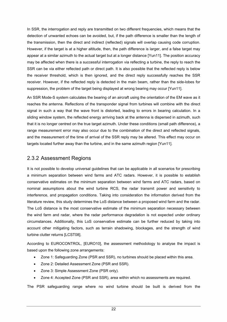
22
In SSR, the interrogation and reply are transmitted on two different frequencies, which means that the
detection of unwanted echoes can be avoided, but, if the path difference is smaller than the length of
the transmission, then the direct and indirect (reflected) signals will overlap causing code corruption.
However, if the target is at a higher altitude, then, the path difference is larger, and a false target may
appear at a similar azimuth to the actual target but at a longer distance [Yun11]. The position accuracy
may be affected when there is a successful interrogation via reflecting a turbine, the reply to reach the
SSR can be via either reflected path or direct path. It is also possible that the reflected reply is below
the receiver threshold, which is then ignored, and the direct reply successfully reaches the SSR
receiver. However, if the reflected reply is detected in the main beam, rather than the side-lobes for
suppression, the problem of the target being displayed at wrong bearing may occur [Yun11].
An SSR Mode-S system calculates the bearing of an aircraft using the orientation of the EM wave as it
reaches the antenna. Reflections of the transponder signal from turbines will combine with the direct
signal in such a way that the wave front is distorted, leading to errors in bearing calculation. In a
sliding window system, the reflected energy arriving back at the antenna is dispersed in azimuth, such
that it is no longer centred on the true target azimuth. Under these conditions (small path difference), a
range measurement error may also occur due to the combination of the direct and reflected signals,
and the measurement of the time of arrival of the SSR reply may be altered. This effect may occur on
targets located further away than the turbine, and in the same azimuth region [Yun11].
2.3.2 Assessment Regions
It is not possible to develop universal guidelines that can be applicable in all scenarios for prescribing
a minimum separation between wind farms and ATC radars. However, it is possible to establish
conservative estimates on the minimum separation between wind farms and ATC radars, based on
nominal assumptions about the wind turbine RCS, the radar transmit power and sensitivity to
interference, and propagation conditions. Taking into consideration the information derived from the
literature review, this study determines the LoS distance between a proposed wind farm and the radar.
The LoS distance is the most conservative estimate of the minimum separation necessary between
the wind farm and radar, where the radar performance degradation is not expected under ordinary
circumstances. Additionally, this LoS conservative estimate can be further reduced by taking into
account other mitigating factors, such as terrain shadowing, blockages, and the strength of wind
turbine clutter returns [LCST08].
According to EUROCONTROL, [EURO10], the assessment methodology to analyse the impact is
based upon the following zone arrangements:
Zone 1: Safeguarding Zone (PSR and SSR), no turbines should be placed within this area.
Zone 2: Detailed Assessment Zone (PSR and SSR).
Zone 3: Simple Assessment Zone (PSR only).
Zone 4: Accepted Zone (PSR and SSR), area within which no assessments are required.
The PSR safeguarding range where no wind turbine should be built is derived from the

23
recommendations provided in the ICAO EUR 015 document [ICAO09], being applicable for any
obstacle within the first cylinder with 500 m radius (more details can be found in Annex A). PSR
designs vary considerably, and the design choices made by PSR manufacturers influence the
susceptibility of their radars to wind turbines. The PSR recommended limit between detailed and
simple assessment is, therefore, derived from the best practices collected from the ICAO EUR 015
document [ICAO09], and the limit is the radius of the cone. When outside the PSR LoS, the impact of
the wind turbine is considered to be tolerable. The information about the PSR recommended ranges is
summarised in Table 2.3.
Table 2.3 – PSR recommended ranges (extracted from [EURO10]).
Zone Zone 1 Zone 2 Zone 3 Zone 4
Description [0, 0.5] km [0.5, 15] km >15 km (within radar
range and LoS) Within radar range
but not in LoS
Assessment Requirements
Safeguarding Detailed
assessment Simple assessment No assessment
The SSR safeguarding range, where no wind turbine should be built, is the same as for PSR, and is
also derived from the recommendations provided in [ICAO09], applicable for any obstacle. The
recommended limit of SSR detailed assessment is obtained from multi target report (for Mode A/C),
and it is based on the conditions to get a reply from a transponder when the interrogation has been
reflected on a wind turbine (the deductions are described in Annex B). Therefore, when the wind
turbine is 16 km away from the SSR, if the airplane is located closer than 5 250 m from the wind
turbine the transponder will not reply to reflected interrogations because of ISLS implementation. In
addition, when further than 5 250 m, the power of the reflected interrogation will be below the
transponder receiver threshold, and the transponder will not reply either. It is to be noted that in the
case of SSR, there is no simple assessment zone. When outside the radar LoS, or further than 16 km,
the impact of the wind turbine is considered to be tolerable [EURO10]. The information about the SSR
recommended ranges is summarised in Table 2.4.
Table 2.4 – SSR recommended ranges (extracted from [EURO10]).
The Simple Assessment (Zone 3) for PSR comprises the following analysis:
Probability of detection, in the shadow region and in a volume located above and around the
wind turbine (due to the large amount of energy reflected that causes an increase in the
radar’s detection threshold).
False Target reports, due to echoes from wind turbines.
The Detailed Assessment (Zone 2) for both surveillance equipment (PSR and SSR) comprises the
Zone Zone 1 Zone 2 Zone 4
Description [0, 0.5] km [0.5, 16] km (within radar
range and in LoS) >16 km or not in LoS
Assessment Requirements
Safeguarding Detailed Assessment No assessment

24
following analysis:
Attenuation in the shadow region and the impact on the radar performance.
False target reports, due to echoes from wind turbines, for all possible scenarios, e.g.,
different wind turbine disposition and characteristics.
False target reports, due to indirect reflections, e.g., reflection of true target echoes on wind
turbines and through reflection of wind turbine echoes on airplane.
Range and azimuth errors, due to small path difference between the direct and reflected
signals.
2.4 State of the Art
The assessment of the influence caused by wind turbines on radar has been widely analysed by the
different ANSPs, to prevent major consequences due to sitting wind farms on radar vicinity and also to
be in acceptance with EUROCONTROL recommendations. According to the European Airspace
Regulator, the assessment should be conducted for each sensor that has at least one wind turbine
within its range coverage. This section shows the research that has been done in the past, highlighting
the added value this Thesis.
The major conclusions that many reports have achieved is that it is not possible to determine an
universally accurate minimum distance where the interactions between a turbine and a radar would
occur, due to the numerous intrinsic variables, such as different terrain profiles, different wind turbine
materials, and wind farm disposition. It is, however, possible to determine a minimum distance where
effects from wind turbines would not be anticipated. So, the assessment needs to be done case-by-
case taking into account all factors described above.
EUROCONTROL has provided some assessment recommendations for ANSP, [EURO10], where
boundaries between a tolerate influence of the wind farms and the need for radar impact assessment
were established, which can be simple or detailed. A set of possible mitigations is also presented:
Wind energy developer mitigations: can the wind turbine proposal be modified to eradicate or
minimise the effects on ATC surveillance systems and operations?
ANSP technical mitigations: can the sensor and/or the surveillance system architecture, be
modified or configured to accommodate the wind energy project to within a level of tolerable
degradation of service to ATC?
ANSP operational mitigations: can ATC modify procedures to accommodate the expected
reduction in surveillance quality?
EUROCONTROL also refers that an important consideration for choosing the mitigation options
should be maintenance of ATC safety and cost-effectiveness.
The authors in [LCST08] provide recommendations for assessing the influence on surveillance
systems, where the results of a study exploring the effects of power reducing wind turbines on Federal

25
Aviation Administration (FAA) ATC radars are described. The report study was performed to identify
mitigation techniques and parameters for such effects, addressing the following topics:
The process for analysing wind turbine and radar electromagnetic compatibility. It includes the
LoS distance between turbine and radar, the terrain shadowing, the methodology for
assessing the effects of turbine clutter returns on radar performance, the effects of shadowing
on detection of desired targets, and the consideration of turbine aggregate effects.
The potential for desired targets to be lost in azimuths other than those of wind turbines (due
to side lobe interaction with turbines).
The consideration of the effects of wind turbines on SSR performance.
The most conservative criteria recommended in this report is a separation ratio between the radar and
the wind farm that exceeds 4/3 smooth, round Earth, with no terrain effects considered. The 4/3 factor
is due to the refractivity of the atmosphere that causes bending of radio waves. This effect can be
taken into account by replacing the true Earth radius by an effective one. Atmospheric refraction varies
widely, depending on the local climate. However, an effective Earth radius of 4/3 times the true one is
representative of the effect of atmospheric refraction under normal conditions. If the wind turbine falls
into that region, supplemented analysis needs to be performed by taking into account the effects of
terrain. The criterion used to assess the impact is based on the increasing of effective noise floor that
could cause desired targets to be lost or generate false targets. The threshold is an interference-to-
noise (I/N) level of -9 dB, less than that will not cause adverse effects. This report also concludes that
the effects of wind turbines on SSR are not expected to differ from those of static structures.
The reports presented by Gavin Poupart, [Poup03] and [Poup06], analyse the impact that different
designs of wind turbines produces on PSR and SSR, respectively, using computational models to
assess this impact, which includes the wind turbine CAD model. He also analyses and compares the
wind turbine echoes for different yaw and pitch angles. The report concludes that the impact of wind
farms can be mitigated by a properly choose of the site, and by choosing materials that absorbs RF
waves. Other reports addressing the problem are studies carried out for real environment, as
presented by Sean Yun, [Yun11], that assess the impact of Riviera wind farm on MSSR at Kingsville
naval air station. Yun did the theoretical assessment and suggested that the wind farm impact on
implemented radars based on four scenarios:
LoS calculation is used to determine potential shadow effect from the turbine.
3D shadow zone created behind the turbine.
False target reports.
Position accuracy which is extremely important for MSSR Mode S.
The report [Hawk09] carried out by FAA examines the impacts to radar coverage from 130 proposed
offshore wind turbines in Nantucket Sound radar, and suggests some recommendations. The major
conclusions reached are the following:
Signal reduction behind the wind farm should have little or no noticeable impact on primary
and secondary radar.
There is a strong likelihood for fading of beacon radar up to 2 NM and primary radar up to

26
3 NM behind the wind farm below an altitude of 600 ft.
There is a marginal possibility that fading of secondary radar could occasionally result in some
missed or garbled replies below 1 000ft over Nantucket for the FMH ATCBI-5 radar, and
below 1 000 ft over Otis from ACK Mode S radar. It is unlikely that these misses will affect air
traffic operations.
There is also a marginal possibility that fading of primary radar could affect primary coverage
below 1 000 ft over Nantucket from FMH ASR-8 radar, and coverage over Otis below 1 000 ft
from ACK ASR-9 radar.
There is a decrease of probability of detection on PSR up to 10%.
The recommendations concern mainly with the equipment update, such as replace the radars and the
displays. The analysis of the Cape Wind farm impact involved Radar Support System, a software
package for radar deploying developed by Technical Services Corporation [Hawk09]. This software is
used to analyse the radar coverage and include terrain data and many radar models.
On the other hand, wind farms stakeholders when proposing the implementation of a new wind farm
need to carried out a report to analyse the impact on surrounding environment and, consequently, in
RF waves, which includes, if exists, the radar assessment on wind farm vicinity.
David Jenn and Cuong Ton discuss in [JeTo12] many methods to predict the wind turbine RCS, citing
their advantages and disadvantages. They present the difference between the rigorous and the
approximated methods for calculate the wind turbine RCS. The report also shows the bi-static and
mono-static RCS for two wind turbine configurations, a vertical axis three-blade design and a vertical
helical design.
Rashid [Rash07] presents the methods used to model individual turbine mono and bi-static RCS using
the standard simplified physical optics far-field RCS approximation of a cylinder. In order to validate
the results, the model was compared to the full physical optics model. On the other hand, Mishra
[MiCh10] also presents a numerical model for a theoretical analysis of the radar signature from a wind
turbine based on the RCS models. To model the radar return from a turbine each blade was assumed
as a cylinder. [Rash07] also presents a proportion of the source of scatter and refers that the strongest
part is derived from the metallic tower, with almost 80%, each blade just contributing with 5%.
NAV Portugal authorises the implementation of wind farms in a radar vicinity if the first and second
Fresnel Ellipsoid are unobstructed for a given flight level and radar range. This Thesis has the purpose
of give other tools to analyse the impact by creating a program to assess the impact created by the
identified wind turbines in the Portuguese radar’s vicinities. The main goal of the simulations is to find
the exclusion regions around the radars, where no wind turbine should be placed.

27
Chapter 3
Model Development and
Implementation 3 Model Development and Implementation
This chapter provides the description of the different models needed to assess the impact of the wind
turbines on surveillance radars, namely the propagation models for the different types of paths, the
models to estimate the wind turbine RCS and the diffraction on the blades, the models to assess the
interference caused by wind turbines on primary and secondary radar signals, and lastly, the flight
routes. The chapter concludes with the simulator description and its assessment.

28
3.1 Propagation Models
3.1.1 Line of Sight
The first propagation situation to be taken into consideration is the LoS between the radar and the
wind turbine; if the distance between the radar and the turbine is greater than the LoS distance, then
the effects caused by the structure should be tolerated. A turbine is considered out of the radar’s LoS
when it is located at a large enough distance; due to the Earth’s curvature, it will be hidden by the
horizon, or when it is obstructed by terrain. One important aspect regarding the LoS analysis is the
diffraction phenomenon due to the Earth’s atmosphere, whose refractivity causes bending of radio
waves and reach far beyond the visible horizon. As suggested in Figure 3.1, the effective height of any
geological formation in the direct LoS reduces its effectiveness at preventing direct LoS [Yun11].
Figure 3.1 – Schematic geometry between a wind farm and a radar at the edge of LoS.
Through a simple mathematical model, the Pythagorean Theorem, it is possible to calculate a
maximum LoS distance between the radar site and any wind turbines in its vicinity, based on the
Earth’s curvature and on the assumption of smooth terrain. The atmosphere’s refractivity effect can be
taken into account by replacing the true Earth radius by an effective one. The atmosphere’s refraction
depends on the local climate; however, an effective Earth radius of 4/3 times the true one ( with
=4/3) is representative of the atmospheric refraction under normal conditions [LCST08]. The
geometric distance to horizon can be computed as follows [LCST08]:
2 , for ≪ (3.1)
where:
is the object radio horizon distance of a smooth, round Earth;
is the height of the object above mean sea level;
is the effective Earth radius (with equal to 6 367 km).
The total LoS between the wind turbine and the radar, using Figure 3.1, is then:
4.12 (3.2)
where:
is the distance from the wind turbine to the radio horizon;

29
is the distance from the radar to the radio horizon;
is the height of the wind turbine;
is the height of the radar.
Thus, LoS methodology represents the most conservative criterion for not anticipating any adverse
effect on the radar, because it uses the 4/3 smooth, round Earth and with no terrain effects. However,
scenarios like those described before are unusual, because the terrain is usually irregular. Therefore,
it is necessary to examine the terrain surrounding the radar for potential shadowing effects, mitigating
any effect of the turbine on the radar. Using a terrain database, it is possible to determine if a certain
area will shadow the turbines from the radar, for which no adverse effects are expected [LCST08].
3.1.2 Diffraction over Terrain
Due to diffraction of radio waves around the terrain, the effective height of the blockage is reduced
from the actual height by the radius of the first Fresnel Ellipsoid. The Fresnel Ellipsoid delimits the
region of space where almost all the energy is present, and its radius is therefore equal to [LCST08]:
(3.3)
where:
is the Fresnel Ellipsoid radius;
is the wavelength of the radio waves;
is the distance from the radar to the blockage;
is the distance from the blockage to the turbine.
Considering the situation illustrated in Figure 3.2, the solid line shows the virtual direct path, and the
dotted lines show the first Fresnel Ellipsoid. The obstruction height can be calculated by subtracting
the radius from the height of the obstacle, being possible to know the attenuation due to the
obstacle using this reduced height for the object [LCST08].
Including the first Fresnel Ellipsoid clearance and terrain data, it is possible to determine how many
wind turbines are in the radar’s LoS. It is assumed that the terrain has a negligible effect on signals
travelling between the turbine and the aircraft, and between the radar and the aircraft. This is
reasonable, since for most of the airspace of interest there will be clear LoS in both cases [Poup06].
The knife-edge model is used to calculate the attenuation due to an obstruction caused by an obstacle
between the radar and the turbine, which should be used when the obstacle’s dimensions are much
larger than the wavelength. For one obstacle scenario, the path loss can be approximated by [Corr12]:
6.4 20 1 , 0.8 (3.4)
in which:
(3.5)
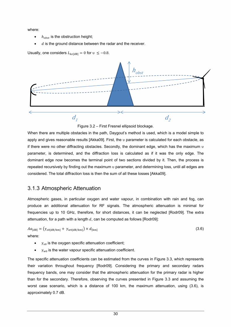
30
where:
is the obstruction height;
is the ground distance between the radar and the receiver.
Usually, one considers 0 for υ 0.8.
Figure 3.2 – First Fresnel ellipsoid blockage.
When there are multiple obstacles in the path, Daygout’s method is used, which is a model simple to
apply and gives reasonable results [Akka09]. First, the υ parameter is calculated for each obstacle, as
if there were no other diffracting obstacles. Secondly, the dominant edge, which has the maximum υ
parameter, is determined, and the diffraction loss is calculated as if it was the only edge. The
dominant edge now becomes the terminal point of two sections divided by it. Then, the process is
repeated recursively by finding out the maximum υ parameter, and determining loss, until all edges are
considered. The total diffraction loss is then the sum of all these losses [Akka09].
3.1.3 Atmospheric Attenuation
Atmospheric gases, in particular oxygen and water vapour, in combination with rain and fog, can
produce an additional attenuation for RF signals. The atmospheric attenuation is minimal for
frequencies up to 10 GHz, therefore, for short distances, it can be neglected [Rodr09]. The extra
attenuation, for a path with a length , can be computed as follows [Rodr09]:
/ / (3.6)
where:
is the oxygen specific attenuation coefficient;
is the water vapour specific attenuation coefficient.
The specific attenuation coefficients can be estimated from the curves in Figure 3.3, which represents
their variation throughout frequency [Rodr09]. Considering the primary and secondary radars
frequency bands, one may consider that the atmospheric attenuation for the primary radar is higher
than for the secondary. Therefore, observing the curves presented in Figure 3.3 and assuming the
worst case scenario, which is a distance of 100 km, the maximum attenuation, using (3.6), is
approximately 0.7 dB.
d1
hobst
d2

31
Figure 3.3 – Specific attenuation for oxygen and water vapour (adapted from [Rodr09]).
These values for atmospheric attenuation and for rain attenuation are low enough to be neglected
(below than 1 dB), because this is an interference problem, and not a coverage one, hence, this
attenuation will affect equally the direct and the reflected signals, therefore, the ratio between the two
power levels will be unaffected by the atmospheric attenuation.
The rainfall intensity for Portugal is relatively low, consequently, for the 3 GHz frequency band the
attenuation due to rain that is not exceeded more than 0.01% of the time is below than 0.1dB.
3.1.4 Spherical Earth Model
The Spherical Earth model is the most accurate one, because it takes the Earth’s radius into account.
Compared to the flat Earth approach, this model shows different results, especially for large distances
[Corr12]. The flat Earth model is the simplest, Figure 3.4, but it is only valid for short distances in
which the Earth curvature is negligible [Pint11]. Furthermore, for the link between the radar and the
wind turbine, and for the assessment distances presented in Chapter 2 (less than 16 km), the
approximated flat Earth model can be used; however, for the link between the radar and the airplane,
or even between the wind turbine and the airplane, the distances can be much larger, and, for those
cases the Spherical Earth must be used.
Figure 3.4 – Flat Earth model.
(3.7)
hr
hair
d

32
where:
is the airplane height;
is the distance separating the airplane from the sensor.
Figure 3.5 represents a schematic for the Spherical Earth model, which solves the problem by
approximating the sphere to a flat model, but with a correction on the radar and airplane heights,
called effective heights. The height correction is related to the distance from the reflection point.
Figure 3.5 – Spherical Earth model.
To calculate the ground distance ( ) between the radar position and the airplane projection, knowing
the position in angles (geographical coordinates), one uses the following expression [Pint11]:
acos (3.8)
(3.9)
where:
is the Latitude of the radar position;
is the Latitude of the airplane position;
is the Longitude of the radar position;
is the Longitude of the airplane position;
is the angle between the radar and the airplane.
The equations necessary to correct the heights of the sensor and airplane are (3.10) to compute the
ground distance between the radar and the reflection point, (3.11) to know the ground distance
between the airplane and the reflection point, and (3.12) and (3.13) to correct the heights. The
equations previously described must be solved in that order. Lastly, (3.7) is used with both heights
corrected to compute the direct distance between the radar and the airplane [Pint11].
32
12 0 (3.10)
(3.11)
2 (3.12)
2 (3.13)
where:

33
is the radar effective height;
is the airplane effective height;
is the ground distance between the radar and the reflection point;
is the ground distance between the airplane and the reflection point.
3.2 Wind Turbine Radar Cross Section
3.2.1 Radar Cross Section Prediction Methods
As described in Chapter 2, the RCS is the only parameter at the radar equation that belongs to the
target, being a measure of how much energy is reflected from a wind turbine, and being very sensitive
to the turbine’s configuration. For example, as the turbine blades rotate, the RCS is likely to change
over several orders of magnitude. This fluctuating RCS means a variable impact on the radar
operation [Poup06].
Many research papers address the importance of correctly describing the wind turbine from the radar’s
viewpoint. The RCS of a point target is defined for an incident plane wave, and according to the IEEE
dictionary of electrical and electronics terms, a measure of the reflective strength of a target defined as
4π times the ratio of the power per unit solid scattered in a specified direction [Grev07].
The determination of the wind turbine’s RCS can be computationally demanding, and there are three
main approaches, i.e., rigorous, approximate, and hybrid solutions methods. The first one includes the
Method of Moments (MoM) solution of integral equations on the frequency domain, the Finite
Difference Time Domain solution (FDTD) of the differential equations in time domain, and the finite
element method that uses the time and frequency domains. The approximate High Frequency
methods (HF) are primarily based on Geometrical Optics (GO) or Physical Optics (PO), and on their
edge diffraction extensions: the Geometrical Theory of Diffraction (GTD) in the case of geometric
optics, and the Physical Theory of Diffraction (PTD) for physical optics [JeTo12]. The high frequency
approximation is used when the target dimension is much larger than the wavelength, as it happen
with wind turbines. There are also hybrid solution methods that can include a mix of the two [JeTo12].
The methods described above require a surface meshing of the wind turbine into small triangular
facets, compared to the wavelength, to find the reflection, diffraction and shadow points. To describe a
wind turbine, hundreds of thousands of facets are required. There are numerous commercial software
tools that can compute the wind turbine RCS, like the High Frequency Structures Simulator by Ansys,
CST Microwave Studio and FEKO [JeTo12].
The computation of RCS without using the computational aids, as CAD models, can be extremely
difficult, not only due to the complex structure, but also due to the degrees of freedom, as the blades
rotation and their position along the time.
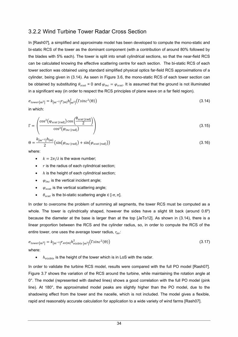
34
3.2.2 Wind Turbine Tower Radar Cross Section
In [Rash07], a simplified and approximate model has been developed to compute the mono-static and
bi-static RCS of the tower as the dominant component (with a contribution of around 80% followed by
the blades with 5% each). The tower is split into small cylindrical sections, so that the near-field RCS
can be calculated knowing the effective scattering centre for each section. The bi-static RCS of each
tower section was obtained using standard simplified physical optics far-field RCS approximations of a
cylinder, being given in (3.14). As seen in Figure 3.6, the mono-static RCS of each tower section can
be obtained by substituting = 0 and . It is assumed that the ground is not illuminated
in a significant way (in order to respect the RCS principles of plane wave on a far field region).
Γ Θ (3.14)
in which:
Γ cos φ cos
θ
2cos
(3.15)
Θ2
sin sin (3.16)
where:
2 / is the wave number;
is the radius of each cylindrical section;
is the height of each cylindrical section;
is the vertical incident angle;
is the vertical scattering angle;
is the bi-static scattering angle ∈[- , ].
In order to overcome the problem of summing all segments, the tower RCS must be computed as a
whole. The tower is cylindrically shaped, however the sides have a slight tilt back (around 0.6º)
because the diameter at the base is larger than at the top [JeTo12]. As shown in (3.14), there is a
linear proportion between the RCS and the cylinder radius, so, in order to compute the RCS of the
entire tower, one uses the average tower radius, :
Γ Θ (3.17)
where:
is the height of the tower which is in LoS with the radar.
In order to validate the turbine RCS model, results were compared with the full PO model [Rash07].
Figure 3.7 shows the variation of the RCS around the turbine, while maintaining the rotation angle at
0°. The model (represented with dashed lines) shows a good correlation with the full PO model (pink
line). At 180°, the approximated model peaks are slightly higher than the PO model, due to the
shadowing effect from the tower and the nacelle, which is not included. The model gives a flexible,
rapid and reasonably accurate calculation for application to a wide variety of wind farms [Rash07].

35
(a) Vertical angles. (b) Scattering angle, top view.
Figure 3.6 – Sectioned turbine for RCS calculations (extracted from [Rash07]).
Figure 3.7 – RCS variation around the turbine (extracted from [Rash07]).
3.2.3 Blades Mono-Static Radar Cross Section
The work in [MiCh10] presents a first-order theoretical model of the radar signature produced by a
wind turbine on S-Band radars [2, 4] GHz, which includes the primary surveillance. As presented in
Chapter 2, the blade is usually composed of a hollow shell of GRP. In some models, within the blade,
there is a conducting wire for lightning protection. According to the Canadian Standards Association,
the wire for the purpose of lightning protection must be at least 4 mm radius [Ridd05]. To model the
radar return from a turbine, each blade can be assumed to be a cylinder of length . Furthermore, for
the PSR operating frequencies, the scattering regime for the lightning wire is optic [MiCh10].
The RCS of a single wind turbine can be formulated by modifying the RCS models of the conducting
or dielectric cylinder [MiCh10], such that it also incorporates the number of blades, the rotational
speed and the dimensions of the turbine. The highly conducting thin cylinder assumption is given by
(3.18), while (3.19) assumes the thin dielectric cylinder.
sin
ln 2 0.5772
(3.18)
1 sin
4 (3.19)

36
where:
2 2 1 / (3.20)
/2 cos 2 2 1 / (3.21)
is the number of wind turbine blades;
is the blade rotation frequency;
is the length of the turbine blade;
is the radius of the cylinder (it is assumed 4 mm);
is the dielectric refractive index (usually 2.7 for solid fibre-glass).
These equations assume that the plane of rotation of the turbine blades is the same as the radar
signal; however, in general, this may not be the case. Assuming that the elevation of the turbine with
respect to the radar is γ, and the angle between the radar’s LoS and the turbine rotor rotation plane is
α, Figure 3.13, the required transformation in the models above will be [MiCh10]:
cos cos (3.22) where:
is the effective blade length.
3.3 Diffraction on the Wind Turbine Blades
It is necessary to have a model to describe the impact of the blades in a bi-static situation. The
primary and secondary radar wavelengths are much smaller than the blade diameter and length,
hence, it is possible to consider blade edges as infinite ones, and apply GTD, i.e., an extension of GO
accounting for diffraction. It introduces diffracted rays in addition to the usual rays of GO, which are
produced at edges, corners, or vertices of boundary surfaces [Kell62].
The initial value of the field on a diffracted ray is determined from the incident field, with the aid of an
appropriate diffraction coefficient. The edge diffraction coefficients, , is determined from certain
canonical problems, and can be computed as follows [Kell62]:
/ /
2 2 sinsec
2csc
2 (3.23)
where:
is the angle between the incident ray and the edge;
is the angle between the incident ray and the normal to the blade;
is the angle between the diffracted ray and the normal to the blade.
Each wind turbine blade has two edges, which can be taken as parallel, therefore, the diffraction
coefficient for the entire blade, , can be assumed as:
/ 2 / (3.24)

37
Figure 3.8 shows the geometry of the problem and the approximation of each blade as two parallel
edges. Note that the x-axis represents the normal to the blade, and the z-axis is along the edge.
Figure 3.8 – Geometry of the rays diffracted on the blade edge.
3.4 Models to Assess the Wind Turbine Influence on Radars
3.4.1 Wind Turbine Shadow Region
If a turbine lies in the radar’s LoS, it generates a shadow region behind it that can degrade radar’s
performance. Therefore, there is possibility that desired targets in the shadow zone can be lost due to
the reduction of the field strength of the radar signal [LCST08]. This section analyses the amount of
shadow created by the wind turbine. Figure 3.9 shows the shadow regions behind the turbine.
Figure 3.9 – Top- (above) and Side-views (below) of wind turbine shadow (extracted from [EURO10]).
The general shape of the shadow is a three-dimensional wedge [LCST08]. It is useful to characterise
the shadow length, height, and width, in order to understand the affected volume behind the turbine.
All the required equations to this characterisation are described in Annex C.

38
If multiple turbines are located within the radar’s main lobe, the size of the shadow zone will also
increase accordingly. These three-dimensional shadows appear in the form of narrow wedges, when
viewed from both a top and side views, stretching beyond the blocking turbine. Targets of interest may
be lost within such a shadow region, due to the reduced field strength of the radar signal, since the full
power of the transmitted signal does not penetrate beyond the blocking wind turbines. Therefore, it is
possible to estimate a minimum flight profile in the wind farm area in order to eliminate the concern
over the shadow region [Yun11].
The impact on the one-way transmission of field strength to a given point in the shadow region
depends, as seen above, on the distances between the transmitter, the turbine, and that point. The
power received via the direct path has to be compared with the one coming via the reflected path.
Therefore, using the relationship between field strength and power loss due to shadow zone, one gets:
1 1 (3.25)
where:
is the attenuation in the shadow region;
is the power via the reflected path;
is the power via the direct path;
is the distance between the radar and the wind turbine;
is the distance between the wind turbine and the receiver;
is the wind turbine tower diameter.
For PSR impact assessment, the possibility of lost targets exists if this shadow region reduces the
strength of a radar return to a level below the noise floor (or sensitivity) of the radar, so that it is
necessary to take this reduction in the field strength into account [LCST08].
3.4.2 Impact on Primary Radar Performance
If a turbine falls into the radar’s LoS, then, it is possible that scattered energy from the wind farm can
adversely affect the performance of the radar receiver by increasing its effective noise floor level. The
occurrence of such increased noise can cause desired targets to be lost, or can possibly even cause
false targets to be generated. The criteria that can be used to assess a threshold for this effect, given
in [LCST08], is the following:
a power level of scattered energy that is less than -9 dB relative to the radar’s noise floor (i.e.,
I/N level that is equal to or less than -9 dB) will not cause adverse effects;
an I/N level that is less than or equal to -6 dB will cause few effects;
levels higher than -6 dB may cause measurable losses in desired targets and can cause the
generation of some false targets.
The following equation can be used to assess whether a wind farm is expected to exceed the -9 dB
(ultra-conservative), and -6 dB (conservative), thresholds, [LCST08]:

39
, ,
4 (3.26)
where:
is the received power (strength of the clutter returns);
is the transmitted power;
, is the transmitted gain for a given direction;
, is the received gain for a given direction;
is the wind turbine radar cross section.
It should be noted that for ATC primary radars, one has and if the radar uses the pulse
compression technique, in (3.26) should be the actual radar transmitted power times the pulse
compression ratio [LCST08]. Moreover, the gain depends on the receiver direction and on the wind
turbine direction; Annex D describes the extrapolation method adopted to compute the gain in any
direction, using the radar horizontal and vertical radiation patterns.
The calculation of the radar receiver’s sensitivity uses the thermal noise level equation [LCST08]:
174 10 log (3.27)
where:
is the noise floor;
is the bandwidth of the radar;
is the noise figure.
Given the I/N degradation at -9 dB, the power threshold for loss of targets is [LCST08]:
9 (3.28)
where:
is the power threshold.
It is desirable that the received power, , is higher than the power threshold, , .
The radar’s MTI processing can remove from the display the effects due to scattered energy from a
wind farm, knowing the wind turbine Doppler signature and applying on radar a software based
spectrum filter [CAA13]. However, a more serious problem, is the problem that energy scattered from
a turbine farm will increase the effective noise floor of the radar receiver, hence, causing desired
targets to be lost in the same azimuth. This effect cannot be mitigated by MTI processing [LCST08].
The scattered energy due to the effect of the time varying blades RCS can exceed the threshold
power. Consequently, in some moments, the turbines will appear in the radar display, being desirable
to know the probability of the scattered energy being above the threshold power and getting caught by
the radar. Therefore, using (3.26) the time that it is exceeded can be computed as follows:
0 (3.29)
where:
is the scattered energy that comes from the wind turbine blades;

40
is the scattered energy that comes from the wind turbine tower.
By solving (3.29) in order of time, it is possible to know the intervals when the threshold is exceeded,
thus, knowing the total time in which the limit is exceeded and the blades rotation period, one has:
(3.30)
where:
is the probability of the scattered energy be above the threshold;
is the period of time in which the scattered energy is above the threshold;
is the wind turbine rotation period.
One should note that does not represent the exact probability of a turbine appearing in the
radar display, because, due to the radar rotation, the radar is not always pointing to the turbine and
also owing to the narrow horizontal beam width, therefore, the period of time that, at least, half power
is transmitted to the turbine can be computed as follows:
2 (3.31)
where:
is the period of time that the radar is pointing to the wind turbine;
is the radar revolution time;
is the horizontal half power beam width.
Consequently, the probability of the radar being pointing to the wind turbine, , is:
(3.32)
Finally, the probability that a wind turbine has to appear in the radar display, , is given by:
(3.33)
As described in Chapter 2, one of the key performance characteristics of a primary radar is the
probability of detection, and this probability is reduced when a turbine increases the effective noise
floor, and generates a false target. This probability can be computed as follows:
1 (3.34)
where:
is the new probability of detection;
is the probability of detection without wind turbine.
Moreover, there is the possibility of creating false echoes in another direction, than in the wind turbine
azimuth, due to a reflection of the radar wave on a turbine. If the reflected wave encounters a nearby
airplane, it can be reflected back towards the radar. However, as seen in (3.26), the dependency of
the received power with distance is very high, being difficult that a wave reflected on the turbine and
on the airplane reaches the receiver above their sensitivity. So, this type of interference can be
neglected [TLC06].

41
3.4.3 Impact on Secondary Radar Performance
Reflections from the turbine can affect the SSR operation for an aircraft in its vicinity. Depending on
the time difference between direct and reflected signals, and on the strength of the turbine reflections,
the possible problems that can occur are split into two categories. The first is when reflected and direct
signals cannot be separated by the receiving system, which can lead to problems such as position
errors and fading (a reduction in signal strength). The second occurs when the reflected signal can be
separated from the direct one, i.e., if the reflected signal is strong enough to create a false target
report, or to corrupt the code of the SSR signal. Figure 3.10 shows the logic used for assessment.
False target or false response reports are due to the implementation of ISLS, the transponder will be
insensitive during 35 µs after receiving the P2 pulse corresponding to a radar interrogation through
radar side-lobes. The problem appears when the P1 pulse reaches the receiver, via reflection onto
wind turbine, after P2 pulses. Therefore, the aircraft will not respond to the interrogation [EURO10].
Figure 3.10 – Impact assessment logic (adapted from [Poup06]).
The major improvements in Mode S are the increased azimuth accuracy, and its interrogation ability.
Unlike other modes, Mode S interrogates one aircraft at a time, and relies on the information of one
reply to determine the target azimuth. Position accuracy is especially important with this mode,
because the interrogation only occurs at the previously recorded bearing for the target. If the bearing
is incorrect, there is a chance that the aircraft will not be interrogated. Reflections of the signal from
nearby objects (such as turbines) will combine with the direct signal in such a way that the wave front
can be distorted, leading to degradation in position accuracy [Yun11].
Position error happens when the following two criteria are met [EURO10]: the difference between
direct and reflected signal strengths is less than system requirement; direct and reflected signals have
a small path difference less than 75 m. Therefore, if the Signal-to-Interference Ratio (SIR) between
direct and reflected signals is lower than a given threshold, errors may occur. In order to compute SIR,
one must know the power levels received by the aircraft via direct and reflected paths. The former,
using free space propagation can be computed as [Corr12]:
4 , , (3.35)

42
which must be above the minimum power required at the receiver,
(3.36)
where:
is the received power via direct path.
is the receiver sensitivity.
The latter can be calculated as described above, assuming that, in the uplink/downlink case, the
received/transmitted gain corresponds to the transponder antenna; as such, the gain will not depend
on the azimuth and elevation, because the antenna is omnidirectional. To compute the reflected power
level, one must consider the power that comes from the tower, coupled with the power that comes
from the three blades. Therefore, the power diffracted on the turbine tower, using (3.17) to compute
the RCS, can be calculated as follows [EURO10]:
, ,
4 (3.37)
Then, the power diffracted on each blade is given by [Elet13]:
, , /
16 (3.38)
where:
1/2 (3.39)
is an index that represents each blade.
As shown in Figure 3.11, the total interfering power for each turbine, , is the sum of the power that
comes from each blade and from the tower:
(3.40)
Figure 3.11 – Interfering powers coming from the turbine.
The SIR for a wind turbine must be computed as follows:
(3.41)

43
where:
is the SIR at the receiver;
In order to ensure that interference will not affect the correct operation of the radar, one must have:
(3.42)
where:
is the minimum SIR required at the receiver.
However, a wind farm can have multiple turbines, placed in different positions, and in the near field of
each other, so, in order to take the effects of all turbines into account, the assessment of interference
is made case by case, and then all interfering signals are added. This approach overcomes the
problem of having different signals with different phases among them, coming from each turbine.
Moreover, this is a worst case design in which synchronisation between turbines does not need to be
taken into account. Therefore, taking only the power level of each interfering signal, as suggested in
Figure 3.12, the total power that reaches to the receiver is given by:
⋯ (3.43)
where:
is the number of wind turbines on the wind farm;
is the interfering power that comes from each wind turbine.
Lastly, the ratio between the direct and all interfering signals coming from the reflection on turbines
can be computed as follows:
∑
(3.44)
Figure 3.12 – Interfering powers coming from a wind farm (worst case).
3.5 Doppler Effect
Other impact in ATC radars performance is the Doppler Effect, which consists on compression or
expansion of signals frequency by a moving object. The frequency shift is computed, for a PSR signal

44
(being half for SSR), as follows:
2 /
λ (3.45)
where:
is the Doppler shift,
is the radial velocity,
Equation (3.45) shows that, as the wind speed increases, the turbines rotate faster producing a larger
Doppler shift. When the wind is blowing perpendicular to the radar main beam it creates a maximum
Doppler shift [Poup03]. Another factor that determines the radar Doppler shift is the angle between the
turbine blades and the radar main beam, which can be computed, for as PSR signal, as follows:
2ω /
λ cos
π2
(3.46)
where:
is the rotation rate of the blades;
is the radar azimuth (measured from North);
is the wind direction (measured from North).
The π/2rad factor present in (3.46) accounts for blades spin perpendicular to wind direction. The
Doppler shift reaches the maximum value when is an odd multiple of π/2 [Amat09].
After computing the frequency shift created by the turbine, it is crucial to know the tolerance of the
radar to these shifts, for the primary radar, the requirement for the frequency tolerance being [CAA12]:
for frequency bands in [2 700, 9 500] MHz the frequency shift must be within 1 250 ppm.
while for the secondary radar, the tolerance must be differentiated between the up- and downlink
cases, the requirements being [ICAO07b]:
for the uplink, the tolerance is ± 0.2 MHz;
for the downlink, the tolerance is ± 3 MHz.
3.6 Flight Routes
The airplane routes are defined by a loxodrome (Pedro Nunes (1502-1578), a Portuguese polymath,
discovered the loxodrome curve during the Portuguese discoveries in the sixteen century), i.e., the
path on a sphere that goes from one point to another always following the same angle. Airspace
routes have many checkpoints, and the angles are the same in-between two contiguous checkpoints,
each route being defined by a specific name and Flight Level (FL) [Pint11].
The navigational charts show the Latitude and Longitude as straight lines (vertical and horizontal), and
for a representation in this way, given the spherical shape of Earth, the distances become distorted,
which depends on the Latitude of the position. Latitudes are parallel circles shrinking in radius away

45
from the Equator, while the Longitude is half of a circle, between the North and South poles, hence, for
each parallel of Latitude (North or South of the Equator) there is a shrinking factor of cos
compared to the Equator; inversely, at a certain Latitude , distances on Earth are stretched by the
reciprocal sec [Alex04].
The angle that defines the loxodrome is different from the one shown in any navigation map. This
happens because the magnetic North is different from the geographical one, the former being the
angle that the navigation equipment measures, and the latter the theoretical angle used in models.
Therefore, any navigational map contains always the magnetic angle, and not the real one, the
relation between them being the declination angle, [Pint11]:
° ° ° (3.47)
where:
is the real route angle;
is the magnetic route angle;
is the declination angle given in relation to West.
The declination angle is provided on all navigational charts, the value changes in time beign different
for different points. The angle that connects two points, A and B, in a Ioxodrome is given by [Alex04]:
arccot∑ ∑
(3.48)
where:
∑ ln (3.49)
The path length ( ) is computed as follows [Alex04]:
| | sec (3.50)
where:
∑ is the vertical spacing of the parallel Latitude .
Since the Longitude defined with West coordinates is negative, it must be taken into account that there
are always two solutions when using trigonometric functions. There is also a specific case, i.e., when
an airplane is travelling always in the same Latitude, for equal to 90° or 270°. Using (3.50), the
distance of the path would be zero, because 0; instead one uses [Pint11]:
sec (3.51)
As mentioned above, sec is the stretching factor depending on the parallel Latitude. If the airplane
travels to the Equator (sec 1), then (3.51) is equivalent to (3.50), with an angle of 0° or 180°.
From the previous equations, one can also conclude that a path can be defined from either a starting
position and an angle, or two different positions. Test routes have a certain number of points in the
path they define, so one must also include the number of test points for each path. The coordinates of
the path separated by a given interval are [Pint11]:

46
1 (3.52)
sec
1 (3.53)
∑ ∑
cot (3.54)
where:
is the distance between fixed intervals;
is the number of points to test in the path;
is the test position, being the initial point for 0, and the final one for 1.
Note that the present in (3.53) and (3.54) is due to the airplane direction. For the Portuguese region,
the Latitude increases to North, while the Longitude increases to East, and decreases to West. So, if
the route is in [0°, 90°], the plus signal must be used to obtain each point Latitude and Longitude,
while if the route is in [90°, 180°], the minus signal is used to obtain the point Latitude, and the plus
one for the Longitude; for the route in [180°, 270°] both coordinates will decrease, therefore, the minus
signal must be used; lastly, for the route in [270°, 360°], the plus signal must be used for the Latitude,
and the minus one for the Longitude.
3.7 Interference Simulator
3.7.1 Simulator Structure and Parameters
In order to analyse the influence caused by the wind turbines on ATC radars, a simulator was created
with the models above described. This simulator estimates the amount of interference produced by the
turbines for different airplane positions. As explained before, the influence of the interference is
different for the two types of radars analysed. The main goal of this simulator is to analyse all
interfering scenarios, for the different airplane routes, and to identify turbines that may cause
measurable interference, and finally estimate exclusion regions. This simulator allows one to analyse
the interference created by future new scenarios that can appear, as new radars or new wind turbines.
Figure 3.13 describes the simulator workflow, which was implemented using MatlabR2013a [MatL13].
First, one describes the system, input parameters and assumptions, then the terrain attenuation
between the radar and the turbine, if they are in LoS; afterwards, the airplane test positions are
described, followed by the algorithm used to analyse the interference, which is differentiated for
primary and secondary radars. For the PSR, the model from Sub-section 3.4.2 was implemented and
for the SSR the model from Sub-section 3.4.3 was used. Finally, there is a results analysis, by
comparing the obtained values with specific thresholds, and, then, there is the definition of the
exclusion regions where no wind turbines should be placed.

47
Figure 3.13 – Simulator general structure.
The simulator requires 5 input files, which are:
the system description, which contains the characteristics of the radar and the wind turbine;
2 files for the radiation patterns, one for the vertical and another for the horizontal, in order to
obtain the 3D radiation pattern (Annex D);
the terrain profile description between the radar and the turbine, which allows to compute the
terrain attenuation and analyse if they are in LoS of each other;
the airplane flight route, the path distance and the number of testing points (Section 3.6).
The files corresponding to the system description and the radar radiation patterns are different if the
assessment is for the primary or the secondary radars. All the other files are generic, and depend only
on the scenario under analysis.
The file that contains the terrain profile between the radar and the turbine was obtained from a script
with Google Maps API Javascript V3 [Java13]. This script was adapted in order to include the
exclusion regions detailed in Sub-section 2.3.2, and all the turbines that fall in these regions. The
different wind farms are displayed with different colours to facilitate the analysis, because the same
wind farm usually has turbines with the same characteristics. The script opens the Google Maps
image and has two input possibilities, which are:
the user select the initial point and the final point in the map;
the user inputs the geographical coordinates of the initial and final points.
The script output is automatically created, and consists of 512 points equally spaced. For each point, it
is shown the distance from the starting point and the respective height. These points are then copied
to a text file (*.txt) to be read by the simulator.
The final output is written in MatLab Command Window, containing, for each test position, the main
results for the interference analysis created by the turbines. The analysis for SSR also includes
graphics with the power behaviour, and the respective SIR along the airplane route.
3.7.2 Local Spherical Coordinate System
The local spherical coordinate system is crucial to implement some basic functions of the simulator:
to obtain the distance between the three points present in this problem; between the radar and
the turbine, between the radar and the airplane, and between the turbine and the airplane;
to know the angles between the radar and the turbine, and between the radar and the
airplane, to compute the transmitted and received gains;

48
to know the angles between the airplane and the radar in relation to the turbine, to implement
the model in Section 3.3, describing each blade, their rotation, and also the rotor rotation, to
compute the diffraction coefficient for each turbine configuration.
Figure 3.14 describes the structure of the algorithm adopted to make the transformation; initially, each
point’s geographic coordinate and height , , is known, therefore, it is necessary to convert to
a universal coordinate system, which is the Earth-Centred, Earth-Fixed (ECEF), then, one has
, , [Koks08]. Thereafter, a point is choose to be the new centre of the referential, e.g., the
turbine, as shown in Figure 3.15 (a). After that, it is needed to rotate the axis from the ECEF axis to
the East, North, Up (ENU) coordinate system, as shown in Figure 3.15 (b) [Sang12]. Finally, the
Cartesian coordinates in relation to the new centre of the referential are converted to spherical
coordinates, , , , in order to have the angles and the distances.
Geographic coordinates and height
Geographic to cartesian coordinates
(ECEF coordinate System)
Referential change
Axis Rotation(ENU coordinate
system)
cartesian to spherical
coordinates
Figure 3.14 – Local spherical coordinate system algorithm.
To change from the universal coordinate system to a local one, Figure 3.15 (a), it follows that:
, , , , , , (3.55)
where:
indexes and mean the reference point and a generic one;
subscripts and mean the local and the universal coordinate systems.
(a) Local Cartesian Coordinates. . (b) ENU coordinate system (adapted from [Sang12]).
Figure 3.15 – Coordinates systems.
Furthermore, to convert from the ECEF coordinate system to ENU, it is necessary to rotate the axis as
described above, therefore, it follows that [Sang12]:
, , , ,2 2
(3.56)
where:
and are the rotation matrices to perform a rotation in the z and x axes.

49
3.7.3 Diffraction Coefficient Algorithm
In order to implement the model from Section 3.3, it is crucial to know the airplane and radar positions
relative to each blade. Therefore, first, it is necessary to know the angles that the airplane and the
radar make with the turbine, after which an axis rotation is applied to describe the other two blades,
which will be 120 ° spaced from each other. Figure 3.16 shows the logical structure of the algorithm.
Figure 3.16 – Algorithm to compute the diffraction coefficient.
The first step is to set the turbine faced to the radar, making the azimuthal angle ( ) equal to zero and
the airplane azimuthal angle, relative to the turbine, is defined as the difference of the other two. Thus,
it is necessary to make an axis rotation of 120° and 240° relative to the turbine axis to know the exact
position of the other two blades; however, rotations are only applied to Cartesian coordinates, so the
spherical coordinates are converted into Cartesian ones. Hence, it follows that:
, , 0 , ,
→, ,, ,
→, ,, ,
→, , , ,
(3.57)
where:
subscripts and represent the radar and airplane coordinates;
the prime symbol represent the coordinates after the rotation;
Finally, after having the correct representation for all the three blades, the model presented in Section
3.3 can be applied using the last coordinate transformation presented in (3.56). Note that this
algorithm should be used for the blades rotation, and for the rotor rotation possibilities, to have the
diffraction coefficient for different turbine orientations, and also to compute the worst case, which is the
maximum value, and the most favourable one, which is the minimum. The movement of the blades
rotation is achieved using a rotation in the x axis, , and the movement to simulate the rotor
rotation is achieved using a rotation in z axis, .
3.7.4 Primary Radar Interference Simulator
The flowchart that represents the primary radar interference simulator is relative to the fourth process
in Figure 3.13, hence, it is assumed that all previous processes are already done, meaning that one
knows the system description, the radar radiation pattern, and the attenuation created by the terrain.
As described in Sub-section 3.4.2, the major impact produced by turbines in primary radars is due to
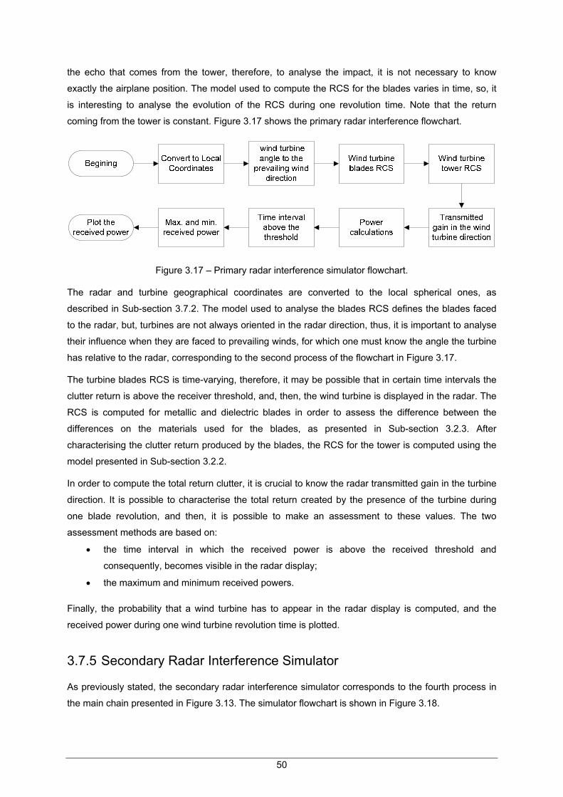
50
the echo that comes from the tower, therefore, to analyse the impact, it is not necessary to know
exactly the airplane position. The model used to compute the RCS for the blades varies in time, so, it
is interesting to analyse the evolution of the RCS during one revolution time. Note that the return
coming from the tower is constant. Figure 3.17 shows the primary radar interference flowchart.
Figure 3.17 – Primary radar interference simulator flowchart.
The radar and turbine geographical coordinates are converted to the local spherical ones, as
described in Sub-section 3.7.2. The model used to analyse the blades RCS defines the blades faced
to the radar, but, turbines are not always oriented in the radar direction, thus, it is important to analyse
their influence when they are faced to prevailing winds, for which one must know the angle the turbine
has relative to the radar, corresponding to the second process of the flowchart in Figure 3.17.
The turbine blades RCS is time-varying, therefore, it may be possible that in certain time intervals the
clutter return is above the receiver threshold, and, then, the wind turbine is displayed in the radar. The
RCS is computed for metallic and dielectric blades in order to assess the difference between the
differences on the materials used for the blades, as presented in Sub-section 3.2.3. After
characterising the clutter return produced by the blades, the RCS for the tower is computed using the
model presented in Sub-section 3.2.2.
In order to compute the total return clutter, it is crucial to know the radar transmitted gain in the turbine
direction. It is possible to characterise the total return created by the presence of the turbine during
one blade revolution, and then, it is possible to make an assessment to these values. The two
assessment methods are based on:
the time interval in which the received power is above the received threshold and
consequently, becomes visible in the radar display;
the maximum and minimum received powers.
Finally, the probability that a wind turbine has to appear in the radar display is computed, and the
received power during one wind turbine revolution time is plotted.
3.7.5 Secondary Radar Interference Simulator
As previously stated, the secondary radar interference simulator corresponds to the fourth process in
the main chain presented in Figure 3.13. The simulator flowchart is shown in Figure 3.18.

51
Figure 3.18 – Secondary radar interference simulator flowchart.
The simulator that analyses the interference starts by defining the local coordinates for the radar,
turbine and airplane, in order to compute the diffraction coefficient for the blades, as described in Sub-
section 3.7.4. Then, the tower radar cross section is computed, to calculate the associated interfering
power. But, to know exactly the amount of energy that reaches the turbine, to compute the interfering
power, and the amount of energy that reaches the airplane via the direct path, one needs to know the
transmitted gain in the desired direction (as described in Annex D). After that, it is possible to compute
the power that arrives to the airplane, via direct and reflected paths, and to compare them. The next
step is to find if the airplane transponder is active or not, because if it is not it does not matter if the
interfering power is above the received one via direct path. Then, it is tested if the difference between
direct and reflected path is higher than 75 m, because, as previously stated, if the distance difference
is less than 75 m, position errors may happen due to signal distortion. Finally, after having the direct
and interfering powers, it is possible to know the SIR, and to compare with specific thresholds in order
to determine if the turbine is creating measurable interference to the correct radar operation. Note that,
for each airplane position, the maximum diffraction coefficient, the minimum one, and the value

52
corresponding to prevailing winds are computed, in order to compare the received power for these
cases and to assess them.
3.8 Model Assessment
In order to make the model assessment, it is essential to present intermediate results. So, for a
primary radar, the most important parameter computed and analysed is the turbine RCS, in this case
from the tower and the blades. Accordingly to EUROCONTROL, [EURO10], the maximum value
assumed for the RCS is 35 dBsm, and for the cases analysed the RCS varies in [27.67, 36.05] dBsm,
which represents that the models used are being correctly applied.
For the secondary radar, the assessment is more complex, due to the model used for diffraction on
the blades. Therefore, two tests were made in order to show the correct implementation of the model.
The first test analyses the behaviour of the diffraction coefficient when the blades rotate in [0°, 360°].
The turbine was defined as faced to the radar, therefore, it is expected that all three blades act the
same way, i.e., the diffraction coefficient is the same with a lag of 120° due to the physical spacing of
120° between each blade. Figure 3.19 (a) shows, as expected, that behaviour, where the periodicity of
the diffraction coefficient is clearly visible.
The second test was to analyse the diffraction coefficient for a rotor rotation between [0°, 360°]. The
blades were defined at 0º. 120º and 240º, and the blades’ plane faced to the radar. As shown in Figure
3.19 (b), it is expected that for the 90º of rotor rotation the diffraction coefficient reaches a minimum,
because at this angle only two blades are visible to the radar and, moreover, for each blade, only one
edge is visible. The maximum value is achieved when the turbine is faced to the radar, i.e., for a rotor
rotation of 0º, 180º and, finally, 360º. As for the blades rotation, the diffraction coefficient for the rotor
rotation is periodic with a period of 180º.
(a) Diffraction coefficient for blades rotation. (b) Diffraction coefficient for rotor rotation.
Figure 3.19 – Diffraction coefficient for the blades rotation and for rotor rotation between [0°, 360°].

53
Besides the noise floor for the secondary radar being -104 dBm, the radar receiver sensitivity -92 dBm
and the transponder sensitivity -74 dBm, Figure 3.20 and Figure 3.21 show the received power even if
they are below these values in order to analyse the impact. These two cases consider that when the
radar is faced to the airplane, because it is the most realistic scenario due to the implementation of
ISLS, when the radar is pointing in another direction than the target, it is supposed that the airplane is
disabled. The distance in the x-axis represents the airplane path, therefore, for each airplane position
the received power via direct path, and the maximum diffracted power from all three blades are
computed (the maximum diffracted coefficient comes from the maximum sum of the blades coefficient,
because it is not realistic to take the individual maximum value once the blades are joined).
Figure 3.20 and Figure 3.21 show that the power received from the direct path is far above all
interference powers. Moreover, in the downlink the difference between the power via direct path and
interference power is less than in the uplink, due to the radar transmitted power, which is ten times
higher than the transponder transmitted power, and, it is also due to the different frequencies used in
the up- and downlinks. It is also possible to see that the power received from the turbine tower is
always below the maximum power diffracted on blades. However, this only happens in this specific
case, because the power diffracted on the blades, when the turbine is faced to another position, will
decrease significantly, as shown in Figure 3.19 (b).
The large variation between the diffracted power from each blade, Figure 3.20 and Figure 3.21, is due
to the fact that the diffraction coefficient changes very quickly. As shown in Figure 3.19 (a), when the
coefficient of one blade reaches the maximum value, for the other two blades it is very low, hence, the
power that comes from the blade that has the maximum coefficient is much larger than the other two.
Figure 3.20 – Radar received power in the downlink.
In this example, blades 1 and 3 are always the dominant component of the diffracted power, the fast
variation that is verified is due to the fact that for each airplane position the maximum of the sum of the
three blades is chosen, and, as seen in Figure 3.19 (a) at 60º, the dominant coefficient changes from
blade 3 to blade 1, and the received power reflects the change in the maximum power diffracted from
one blade to another.

54
Figure 3.21 – Airplane received power in the uplink.
In the chosen path, the airplane is moving towards the radar, thus, it is expected that the received
power increases as the airplane comes closer, which can be seen in Figure 3.20 and Figure 3.21.
Figure 3.22 shows an example of the terrain attenuation, computed by Daygout’s method, as
described in Sub-section 3.1.2. For the operation frequency of 1 090 MHz, the computed result gives
22.28 dB of attenuation. The manual verification of this result is the following:
is equal to 65 m;
is equal to 8 700 m;
is equal to 13 826 m.
Figure 3.22 – Terrain attenuation example.
Therefore the dominant edge has 2.999, and, consequently, 22.19dB, which gives a very
reasonable approximation of both results.

55
Chapter 4
Analysis of Results and
Definition of Exclusion Regions 4 Analysis of Results and Definition of
Exclusion Regions This chapter starts by presenting NAV Portugal’s surveillance equipment used in this Thesis. Section
4.2 shows the different scenarios under analysis, followed by Section 4.3, which describes the Doppler
impact on the radar. Section 4.4 analyses the simulation results for the various scenarios, thus,
leading to the practical method to estimate exclusion zones presented in Section 4.5.

56
4.1 NAV Portugal’s Surveillance Systems
This section presents the surveillance radars managed by NAV Portugal. Their main mission is to
provide air traffic services in the Flight Information Regions (FIR) under Portuguese responsibility –
Lisbon and Santa Maria, Figure 4.1. The management of an airspace with the size of the Portuguese
one, with an area around 6 million km2 (approximately 60 times the national territory, i.e., equivalent to
an area larger than Europe), the largest one in Europe, and one of the largest in the world, requires
surveillance systems with high reliability [NAV13a].
Figure 4.1 – Portuguese Flight Information Regions (adapted from [IMAG13]).
In accordance to EUROCONTROL in surveillance standard document used until recently [EURO97],
the radar coverage required to support both terminal and en-route air traffic services should have
double SSR coverage, which means that, for a given point in space, the radar data used by an ATS
unit for the surveillance function are derived from, at least two, independent SSR sources working
simultaneously. The same EUROCONTROL recommendations established that the antenna
revolution time could go up to 4 s for TMA and to 12 s for En-route airspace. As shown in Figure 4.2,
NAV Portugal has seven SSR, one PSR (co-located with SSR in Lisbon Airport) and two surface
radars to respond to these requirements. Figure 4.2 shows the geographical radar distribution as a
function of the different airports. Nowadays, the recommendations are based on the quality, and
capacity of coverage, and not the quantity of surveillance sensors, present in the specification for ATM
Surveillance System Performance, released on March 2012 [EURO12b]. The changes on
recommendations are due to the introductions of new surveillance systems as ADS-B, and WAM.
Portugal’s mainland has one radar in the northern region, not only to ensure coverage there, but also,
to ensure effective approach and landing monitoring at the international airport of Porto. Two other
radars are in the centre, to guarantee the correct ATC at the Lisbon airport, the Lisbon’s radar is
responsible for the approach, and Montejunto’s radar to en-route monitoring. Two radars are
responsible for the surveillance on southern region, and Faro airport uses the Faro’s radar for
approach, and Foia’s radar for en-route. There is also one radar in S. Maria Island, in Azores, and
another in Porto Santo, in Madeira. Table 4.1 describes the different functionalities of Portuguese
surveillance radars and their position, more detailed characteristics can be found in Annex F.

57
Figure 4.2 – Surveillance radars in Portugal (Extracted from Google Maps).
As shown in Table 4.1, the surface radar is part of the surveillance system situated in Lisbon and
Porto airports. This type of radar sensors are used to monitoring the activity surrounding, or on critical
infrastructure areas, such as airports, seaports, military installations, national borders, refineries, and
other critical industries. Such radars are characterised by their ability to detect movement at ground
level of targets, such as an individual walking, or crawling towards a facility. Such radars typically have
ranges from several hundred metres to over than 10 km. The carrier frequencies range goes from the
X (about 10 GHz) to W bands (about 77 GHz). The study of the interference caused by turbines on
this kind of radar is not required, because, as referred in Chapter 2, the definition of BRA excludes the
implementation of any turbine in 500 m from the radar.
In order to ensure the uninterrupted provision of radar services on the widest possible scale, as well
as the application of specific radar separation standards, it is essential to have comprehensive and
continuous radar coverage of high quality and reliability. This may be achieved either by optimising the
use of existing facilities, by installing new radar facilities, or by sharing the use of radar stations.
Sharing radar data enables to maintain the redundancy of the radar services, at a level compatible
with efficiency, and to avoid costs duplication [EURO97].
Portugal receives data from Spanish radars, such as the Aspontes, Cancho Blanco, and Valladolid,
and shares the radar data with AENA, Spanish ANSP, and ONDA, Morocco’s ANSP [Pere11]:
Fóia – To AENA (Sevilla) and ONDA (Casablanca).
Montejunto – To AENA (Madrid).
Porto Santo – To AENA (Canárias) and ONDA (Casablanca).
From AENA – Cancho Blanco, As Pontes and Valladolid.

58
Table 4.1 – NAV Portugal surveillance radars (Extracted from [Pere11]).
System Purpose Location
Secondary Surveillance Radar Approach Lisboa
En-Route Montejunto
En-Route Foia
Approach Porto
Approach Faro
En-Route P. Santo (Madeira)
En-Route Sta. Maria (Azores)
Primary Surveillance Radar Approach Lisboa
Surface Surveillance Radar Ground Lisboa
Ground Porto
A crucial parameter for the ATC is the minimum vertical and horizontal separations between airplanes
to keep safety. The minimum vertical separation between aircrafts is 1 000 ft (300 m), and the
minimum horizontal radar separation applied within Lisbon FIR/UIR is 8 NM, except in the areas
mentioned below, where the following minimum separation is applied (a vectoring area corresponds to
the space where airplanes perform manoeuvres for the final approach to the airport) [NAV07]:
5 NM within the Lisboa Airport Radar Vectoring Area.
7 NM within Porto Radar Vectoring Area.
10 NM within Faro TMA and Madeira TMA.
20 NM within Madeira Sector.
For Santa Maria FIR, the following minimum horizontal radar separation is applied:
10 NM within a volume up to 100 NM from Santa Maria Radar Antenna, and below FL 245.
20 NM elsewhere within a volume of 200 NM, centred on Santa Maria Radar Antenna.
According to the rules and procedures defined by the Portuguese Airspace regulator, for the flight
level at approach, or the flights where the aircraft remains in visual contact with the airport, the
airplane must maintain a minimum height of 1 000 ft above the highest obstacle round a radius of
600 m. On route, the airplane must maintain a minimum height of 2 000 ft (600 m) above the highest
obstacle located within 8 km each side of the route stated in the Flight Plan [NAV11].
4.2 Scenarios Definition
The turbines that fall into the interference zone established in Chapter 2 define the different scenarios.
Each turbine is located at a different distance from the radar, has a different structure, leading to
different propagation environments, and to distinct influences. Using Google maps and the
INEGI/APREN report, [ENEG11] on all wind farms in Portugal, one has collected their location within

59
the interference radius (16 km), accordingly to the radars locations:
Foia: 1 wind farms;
Montejunto: 5 wind farms;
Lisboa: 6 wind farms;
Sta. Maria: 1 wind farms;
P. Santo: 1 wind farms.
Neither the Porto nor the Faro radars have any turbine in the interference zone. In Figure 4.3, one
shows in red the 500 m safety range, where no turbine should be placed, and in blue the 16 km
interference radius. Within this radius, one found 81 different turbines distributed by 14 wind farms.
For each turbine, it is crucial to get the terrain profile, in order to analyse the terrain attenuation. If
there are some turbines that have a similar terrain profile, the interference analysis is performed for
only one turbine, and then, it is assumed that the other turbines create the same attenuation.
Table 4.2 summarises the information for the scenarios identified for the different radars, presenting
the number of turbines, distributed by the different wind farms, and their main characteristics, as the
average distance to the radar, the height of the tower, and the blades length. The marker colour
column presented in Table 4.2 corresponds to the colours used to distinguish between the different
wind farms in Table 4.3. The individual turbine geographical coordinates can be found in Annex E.
Table 4.2 – Wind Farms within the interference radius for the different radars.
Radar Wind Farm Marker Colour
Number of Turbines
Wind Farm distance [km]
WT Height [m]
WT blades
length [m]
Foia Madrinha Blue 5 2.00 64 35.5
Montejunto Alto da Folgorosa
Blue 9 8.85 80 46.0
Joguinho Green 14 12.05 59 41.0
Achada Orange 3 14.50 80 45.0
Caldas Light blue 5 13.95 67 41.5
Serra de Todo-o-Mundo
Light green 5 13.20 60 40.0
Lisbon Almargem Orange 3 14.10 78 41.0
Bolores Pink 4 13.30 45 31.0
Sardinha Blue 13 14.50 67 43.5
Valérios Red 1 14.80 59 41.0
Fanhões Brown 9 13.70 60 40.0
V. Franca de Xira
Yellow 4 14.25 80 44.0
P. Santo Cabeço do Carvalho
Pink 3 4.55 55, 30 23.5, 14.5
S. Maria Figueiral Pink 3 4.95 44 15.0

60
(a) Scenarios in Foia radar. (b) Scenarios in Montejunto radar.
(c) Scenarios in Lisbon radar. (d) Scenarios In S. Maria radar.
(e) Scenarios in the P. Santo region. (f) Link between Lisbon radar and one turbine.
Figure 4.3 – Scenarios identified.

61
The model used to analyse the interference caused by a turbine on a secondary radar needs to know
the airplane position, therefore, it is necessary to test the scenarios for the most probable airplane
position, which correspond to the Flight Routes (FRs) in the Portuguese airspace. For these FRs four
different heights where chosen:
1 000 ft (300 m) to simulate the approach to the airport (as defined in Section 4.1, this is the
minimum safe altitude above the highest obstacle).
5 500 ft (1 700 m), corresponding to the FL 55, which is the minimum controlled altitude
outside the TMA.
15 000 ft (4 600 m), corresponding to the FL 150 which is an intermediate level.
30 000 ft (9 100 m), corresponding to the FL 300 which is the most common En-route height.
The chosen FR for testing the interference depends on the radar region, consequently, the routes that
are in the radar vicinity are chosen, i.e., approximately 50 km. The Terminal Area Charts of the
different airports provided by NAV [NAV13b] were used. Annex G provides the geographic information
about the routes chosen.
Table 4.3 shows the FR that has been picked up to test the scenarios. Moreover, Faro and Porto
radars do not have turbines in the interference region, however, one tested the possibility of existence
of turbines in the highest hills, in order to create the exclusion regions for these radars. The airplanes
follow the signals that come from the VHF Omnidirectional Radio Range (VOR), therefore, the FRs are
defined by an initial and a final VOR, as shown in Table 4.3.
One important parameter in the turbine interference issue is the most probable blades orientation,
which leads to an analysis to the prevailing winds. Figure 4.4 shows the wind direction distribution for
all year, and allows concluding that the prevailing wind direction is North-NorthWest (NNW).
Therefore, the wind turbine interference analysis is performed for the blades orientation that causes
more interference, and for the blades orientation accordingly to the prevailing winds, to make a
comparison between both.
Figure 4.4 – Wind direction distribution (extracted from [Wind13]).

62
Table 4.3 – FRs chosen for the different radars.
Radar FR [Degrees]
Initial Coordinates [Degrees]
Initial VOR Final VOR Route distance [NM]
Foia 330 37.013, -7.975 Faro Odemi 45
036 37.307, -9.000 Sunes - 35
170 37.497, -8.383 Usalo Odemi 17
221 37.597, -7.950 Xapas Usalo 28
Lisbon and Montejunto
218 39.665, -8.492 Fátima Lisboa 56
208 39.665, -8.492 Fátima Espichel 81
175 39.665, -8.492 Fátima Magum 30
203 39.167. -8.392 Magum Ateca 32
223 39.167, -8.392 Magum Adsad 58
231 39.167, -8.392 Magum Dekus 30
069 38.887, -9.162 Lisboa Magum 40
077 38.887, -9.162 Lisboa Olgar 60
214 38.887, -9.162 Lisboa Odlix 15
246 38.887, -9.162 Lisboa Busen 44
P. Santo 036 33.090, -16.350 P. Santo Lidro 40
052 33.090, -16.350 P. Santo Rakun 40
067 33.090, -16.350 P. Santo Degun 40
192 33.090, -16.350 P. Santo Tabom 52
220 33.090, -16.350 P. Santo Madat 67
307 33.090, -16.350 P. Santo Irsan 9
S. Maria 066 36.962, -25.166 S. Maria Bekun 10
088 36.962, -25.166 S. Maria Dokas 10
131 36.962 -25.166 S. Maria Etrox 10
262 36.962 -25.166 S. Maria Ginsu 10
282 36.962, -25.166 S. Maria Gomos 10
310 36.962, -25.166 S. Maria Aspex 10
342 36.962, -25.166 S. Maria P. Delgada 10
4.3 Doppler Effect Impact Assessment
Using the information presented in Table 2.2, three different scenarios were identified to analyse the
Doppler Effect impact created by the turbines on ATC radars, namely, the variations of rotor angle
relative to the radar, blade length, and rotation speed. As shown in (3.45), there is a trade-off between
the blade length and the rotation speed, therefore, the two extreme cases were analysed:

63
the 44 m rotor diameter, with a maximum rotation speed of 34 RPM;
the 100 m rotor diameter, with a maximum rotation speed of 13 RPM.
First of all, it is interesting to make the analysis of the radial velocity in the blade edge, therefore, for
the 22 m blade length, with a maximum rotation of 34 RPM, the maximum radial velocity is
78.3 rad/ms, i.e., 281.88 km/h. For the 50 m blade length, with a maximum rotation of 13 RPM, the
maximum radial velocity is 68 rad/ms, i.e., 244.8 km/h.
Figure 4.5 shows the Doppler shift for rotor rotation [0°, 360°], for the secondary radar. At 0°, the
turbine is facing the radar, in which case there are no changes in frequency, however, when the rotor
is perpendicular to the radar, the higher Doppler shift is produced. Figure 4.5 also shows that smaller
turbines, with a higher rotation speed, create a great deviation in frequency; moreover, the downlink
case (dashed lines) produces a larger shift than the uplink one (solid lines).
Figure 4.5 – Doppler shift produced by a wind turbine on the Secondary Radar.
Figure 4.6 shows the Doppler shift impact at primary radar frequency bands, for a rotor rotation in
[0°, 360°]. As for the secondary radar, the smaller turbines (blue lines) produce a larger Doppler shift,
because they spin faster; moreover, for the frequency band of 2 840 MHz, the frequency deviation is
also higher, because, as seen in (3.44), the Doppler effect is proportional to the radar frequency.
For the secondary radar, the highest value for the Doppler shift is 284.6 Hz, for the 22 m blade, in the
downlink, and for a rotor rotation of 90°. As previously presented in Section 3.5, the tolerance for the
frequency deviation is 0.2 MHz and 3 MHz for up- and downlinks, respectively, therefore, the
5.69 10-4 MHz computed for the Doppler shift is far below from these values.
For the primary radar, the highest value is 1 483 Hz, for the 22 m blade, and for the 2 840 MHz radar
frequency, and also for a rotor rotation of 90°. The tolerance for the frequency deviation is 1 250 ppm,
which means that, for 2 760 MHz the tolerance is 3.45 MHz, and for 2 840 MHz it is 3.55 MHz.
Therefore, it can be said that the maximum Doppler shift computed for the primary radar frequency
bands are considerably below the tolerance values.

64
Figure 4.6 – Doppler shift Produced by a wind turbine on the Primary Radar.
The results obtained for the frequency shift allow to state that the Doppler shift produced by wind
turbines will not be a problem for the radar signals reception viewpoint, because the tolerance values
are never exceeded. However, for the PSR operation, and due to the high radial velocity at the blade
edge, the frequency shift produced can be similar to an aircraft, therefore, the MTI can recognise as a
target, showing the wind turbine in the display.
4.4 Interference Simulator Results
4.4.1 Primary Radar
Using the data from Table 2.2 concerning the maximum turbine rotation frequency, and from Table 4.2
regarding the main characteristics of each turbine that falls in the interference zone, it is possible to
measure the impact caused by each turbine in the primary radar.
The main characteristics of the radar are:
peak power of 1.2 MW (90.71 dBm);
sensitivity of -106 dBm;
transmitted gain in the main lobe direction is 33.5 dBi, and the gain in the desired direction is
obtained as explained in Annex D;
tilt of 2.8°;
half power beam width of 1.45°.
The radar height above the ground is 36 m, and the terrain profile between the radar and the turbine
was extracted from Google Maps, as described in Chapter 3.
The results from the simulations are distributed by the different wind farms, and within the farms the

65
numbering of turbines starts with the closest one to the radar. First, two tables are presented for one
tested scenario, in order to compare the maximum and minimum received powers for the different
possibilities, i.e., for the different blades material, and for the different radar operation frequency, to
understand the influence of these parameters on the results. Thereafter, the simulations done to each
turbine that was described in Section 4.2 are presented, and for each case the worst result is shown.
The results are divided in two tables, one being for the turbines that always cause interference on the
primary radar, because the received power is above the radar sensitivity, and the other being for the
turbines that have periods where the scattered energy is above the radar threshold.
The first analysis is to understand the impact produced in the received power by different materials for
the blades, for different turbine orientations, and for different radar operation frequencies, therefore, a
wind turbine in Almargem was chosen, without terrain attenuation, to make the assessment. Table 4.4
and Table 4.5 show the maximum and minimum received power for the different combinations.
Table 4.4 – Maximum received power from a wind turbine in Almargem.
WT Orientation
Maximum received power [dBm]
2 760 MHz 2 840 MHz
Metallic Dielectric Metallic Dielectric
Radar -34.48 -33.46 -48.17 -47.45
NNW -31.59 -41.92 -51.19 -51.15
Table 4.5 – Minimum received power from a wind turbine in Almargem.
WT Orientation
Minimum received power [dBm]
2 760 MHz 2 840 MHz
Metallic Dielectric Metallic Dielectric
Radar -41.96 -41.96 -51.31 -51.31
NNW -41.96 -41.96 -51.31 -51.31
Concerning the blades material, it is noted that for the maximum received power, the difference
between metallic and dielectric blades is always below 1 dB. For the minimum received power, there
is no difference between the materials used. One can conclude that the dielectric blades will lead to a
higher value of scattered energy, thus, being the worst case.
Regarding the radar operation frequency, it can be observed that the difference between the 2 760
and 2 840 MHz bands is quite high, reaching, in some cases, values above 10 dB. For the maximum
received power, Table 4.4, the difference in results between the two frequency bands is higher than
the difference for the minimum received power, Table 4.5. This high difference can be explained by
the frequency dependence of (3.18) and (3.19), therefore, the higher the frequency, the lowest the
blades RCS, and, consequently, the received power.
Finally, regarding the impact of the turbine orientation in the received power, it is shown that, for the
metallic blades at 2 760 MHz, the difference is around 3 dB, which means twice the received power

66
when the turbine is pointing to the prevailing winds. For dielectric blades, the orientation leads to a
difference over than 8 dB. The difference in the received power due to the orientation is around 3 dB,
when the radar operates at 2 840 MHz. Using this example, it can be concluded that, for minimising
the impact of turbines in the primary radar, the best radar operation frequency is 2 840 MHz.
Table 4.6 shows the simulation results for all the turbines that always cause interference on the radar,
because the scattered energy is always above the radar threshold. It was observed that these wind
turbines are in LoS, which means that there is no terrain attenuation between the radar and the
turbines. The results show the worst case for each turbine, as the maximum and minimum received
powers, the orientation which led to the worst case, the blade type, the distance to the radar, and the
radar operation frequency.
The turbines are at a distance in the range [12.62, 15.56] km, and cause a maximum radar received
power in [-37.95, -28.60] dBm, and a minimum received power in [-37.26, -57.71] dBm. The turbines
are placed in the azimuth in [-53.5°, 8.5°] measured from North, therefore, the degradation in the radar
performance can occur in this azimuth interval. The turbine RCS is in [27.67, 36.05] dBsm. About
51.7% of the turbines produce more scattered energy when the radar operation frequency is
2 760 MHz, and the remaining 48.3% when the radar operation frequency is 2 840 MHz. The worst
blade material is usually the dielectric, but the difference in relation to the metallic blades is very small,
less than 1 dB. The usual orientation that leads to a higher received power is NNW, however, note
that the values obtained are peaks, which does not mean that the dielectric blades, or the orientation
to the NNW, lead to a higher average scattered energy.
Table 4.7 shows the simulation results for the turbines that sometimes cause interference to the radar,
located in Sardinha’s wind farm, because in some time intervals the scattered energy is above the
receiver threshold. The difference relative to the results from Table 4.6 is the fact that these turbines
are not in LoS. Moreover, the terrain attenuation is frequency dependent, therefore, for higher
frequency values, the higher the terrain attenuation. Table 4.7 shows the worst case, corresponding to
the highest received power, thus, to the lowest terrain attenuation. Therefore, if there is terrain
obstruction between the radar and the turbine, higher frequency values will lead to a higher value for
the attenuation.
With terrain attenuation, it is noted that the minimum received power decreases significantly, going
below the receiver threshold. Note that the terrain attenuation affects the signal twice, because it is a
PSR signal. For these cases, it is interesting to know the probability of interference. The probability of
the scattered energy being above the threshold is, for the first four turbines, about 48%, while for the
last turbine it is 99%. This means that the probability of detection of a desired target in the same
azimuth as the wind turbine is affected. These values represent a decrease of the detection probability
of 0.2 %, and 0.4 %, respectively. Note that for the results presented on Table 4.6, the received power
is always above the threshold, therefore is 100 %. The strong variations between the minimum
and maximum received powers due to the blade rotation will appear as flashes in the radar screen.
Consequently, this amount of scattered energy will cause an increase in the radar’s detection
threshold, in the resolution cell where the wind turbine is located [EURO10].

67
Table 4.6 – Simulation results for the WT that always cause interference to the primary radar.
Wind Farm
Dist.
[km]
Orientation Angle to NNW
[Degrees]
Min. Power [dBm]
Max. Power [dBm]
Max. RCS
[dBsm]
Radar Freq. [MHz]
Almargem 13.97 NNW 31 -41.96 -31.59 32.97 2 760
14.1 NNW 30 -44.06 -31.82 32.90 2 760
14.23 NNW 29 -43.76 -30.63 34.49 2 840
Bolores
12.95 NNW 12 -43.07 -30.47 33.02 2 840
13.05 NNW 14 -51.02 -31.03 32.35 2 760
13.39 NNW 14 -51.05 -31.49 32.33 2 760
13.59 NNW 14 -41.28 -31.26 32.82 2 760
Sardinha 13.82 Radar 9 -38.93 -28.97 35.40 2 760
14.39 Radar 9 -44.45 -30.36 34.71 2 760
14.91 NNW 8 -50.99 -31.11 34.58 2 760
14.83 NNW 7 -42.06 -29.79 36.05 2 840
14.64 NNW 6 -43.09 -34.11 31.26 2 760
14.68 NNW 4 -57.71 -31.12 34.55 2 840
14.64 Radar 3 -44.50 -37.95 27.67 2 840
15.14 NNW 3 -49.82 -31.29 34.67 2 760
Valérios 14.82 Radar 2 -51.69 -36.30 29.53 2 840
Fanhões 12.62 NNW -20 -37.26 -28.60 34.44 2 840
12.93 NNW -21 -40.66 -33.14 30.07 2 760
12.98 NNW -21 -38.86 -29.24 34.29 2 840
13.51 NNW -23 -41.41 -31.08 33.15 2 840
13.99 Radar -21 -43.46 -29.49 35.34 2 840
14.12 NNW -19 -39.31 -31.28 33.47 2 760
15.56 NNW -20 -40.17 -31.88 34.80 2 840
14.71 Radar -19 -39.12 -30.16 35.54 2 840
14.70 NNW -19 -37.63 -31.52 33.92 2 760
V. F. Xira 13.98 NNW -30 -38.63 -29.87 34.95 2 840
14.26 NNW -30 -44.59 -31.29 33.63 2 760
14.37 NNW -31 -40.91 -30.13 35.17 2 840
14.50 NNW -32 -42.97 -31.09 34.12 2 760
From the simulations, it can be stated that the presence of wind turbines can affect radar operation in
the same azimuth where they are, hence, the probability of detection can be compromised in these
azimuths. According to EUROCONTROL, [EURO10], a 3 dB of attenuation in the shadow region will
affect a volume of 1 600 m behind the turbine, with 310 m of height and 45 m of width. This shadow
region is sufficiently small to be tolerable by the PSR. Moreover, this attenuation will not affect the
radar, because commercial aviation is always above than 1 000 ft (300 m), as defined in Section 4.1.

68
Table 4.7 – Simulation results for the WT that sometimes causes interference to the primary radar.
Dist.
[km]
Blade type
Orientation
Min. Power [dBm]
Max. Power [dBm]
Radar Freq. [MHz]
[dB]
13.82 Die Radar 0.4792 0.2 -134.3 -75.93 2 760 22.35
13.81 Die Radar 0.4793 0.2 -142.8 -83.20 2 760 25.93
13.84 Die Radar 0.4972 0.2 -158.2 -98.18 2 760 33.46
13.86 Die Radar 0.4970 0.2 -137.8 -76.66 2 760 22.69
13.83 Die NNW 0.9990 0.4 -123.9 -56.17 2 760 12.18
4.4.2 Secondary Radar
Using the data from Table 4.2 to know the main characteristics of each turbine that falls in the
interference zone, and from Table 4.3 to define the airplane path, it is possible to measure the impact
caused by the wind farms in the secondary radar. The specific radar characteristics, as the tilt, the
height above ground, and the geographical coordinates, are shown in Annex F. The terrain profile was
extracted from Google Maps, as described in Chapter 3. The analysis is done for each km of the
airplane path. The impact is differentiated between the uplink, in which the radar is the transmitter and
the transponder is the receiver, and the downlink, which is the other way around. Therefore, the main
characteristics used to characterise the radar and the transponder are:
transmitted power of 63 dBm for the radar, and 54 dBm for the transponder;
sensitivity of -92 dBm for the radar, and -74 dBm for the transponder;
minimum SIR of 10 dB and 20 dB for the conservative case;
transmitter gain in the main lobe direction of 27 dBi, and the gain in the desired direction is
obtained as explained in Annex D.
There are two different possibilities that a turbine produces interference in a secondary radar, the first
one being when the radar boresight is pointing to the airplane, and the second when the radar is
pointing to the turbine. As shown in Figure 4.7, and as expected, when the radar is pointing to the
airplane, the direct received power is far above the interfering power. However, when the radar is
pointing to the turbine, and due to the high directivity of the radar antenna, the received power is
below the interfering power. Therefore, for the first case, the SIR is above the two thresholds, and for
the second case, the SIR is below the thresholds. However, the second case does not create
interference problems due to the ISLS implementation.
The maximum interfering power is obtained, as described in Sub-section 3.4.3, with the contribution of
the power reflected on turbine tower, and the power diffracted on the blades. The maximum interfering
power that comes from the blades is due to the maximum value for the diffraction coefficient.
Therefore, it was necessary to get, for all the possibilities of wind turbine orientation in [0º, 180 º], the
blades position that leads to the maximum diffraction coefficient. The reason for the strong variation of
the SIR in downlink is mainly due to the fast variation of the blades diffraction coefficient, causing

69
strong variations in the interfering power. Moreover, in downlink, the whole turbine is visible, which
causes a higher interference, the transmitted power is much lower and frequency is 60 MHz higher.
Figure 4.7 – SIR for S. Maria wind farm and for FR 131 and FL 150.
The increase, or, decrease of SIR behaviour depends on the airplane route, because, as shown in
(3.35), the direct power decreases with the square of the distance, and the interfering power
decreases as well as the square of the distance between the transmitter and the turbine, but
decreases also with the square root of the distance between the turbine and the receiver, as shown in
(3.38). The SIR is also very affected by the turbine diffraction coefficient, because the direct signal has
a constant behaviour, increasing, or, decreasing, depending on airplane route, but the interfering
power is dependent on the diffraction coefficient.
Note that the values obtained for SIR are very high, therefore, the probability of decreasing below the
thresholds is very low. Moreover, the chance of the turbines causing more interference is when they
are in the same azimuth as the airplane path, because, in this situation, the horizontal gain in both
directions is similar. Consequently, when the radar is pointing to the airplane, for the case when the
wind turbines do not lay in the airplane route, the SIR is always above the receiver threshold.
The impact of the turbine pointing to prevailing winds (NNW) is shown in Figure 4.8. It is possible to
see, as expected, that when the turbine is oriented to another direction than the one that leads to a
maximum interfering power, the SIR is higher. Moreover, the larger the angle between the maximum
of the diffraction and orientation to NNW, the smaller the diffraction coefficient, and, consequently, the
interfering power. The general SIR behaviour is the same for both received powers, only changing the
value for the diffraction coefficient.
First, the impact caused by the different FR in the received SIR was analysed, when the radar is
pointing to the airplane, the results are shown in Table 4.8. For this analysis, the wind farm in S. Maria
was chosen, because the three wind turbines lay in the same azimuth relative to the radar. It is
possible to see that for all cases the SIR is far above the thresholds. The most critical FRs, which
have the lower SIR, are FR 066, FR 088 and FR 282, these routes having in common the fact that the
azimuth close to the turbines. In the case of FR 066 and FR 088, the route passes over the turbines

70
and the radar.
Figure 4.8 – SIR for S. Maria wind farm for turbines faced to NNW using FR 131 and FL 150.
The impact of the different FLs in the received SIR is assessed from Table 4.8, where it is possible to
see that the worst FL for the FRs that are closer to the turbine azimuth is the lower one, FL 10. For the
other FRs, because they pass over the radar and the turbine, the worst FL is the highest one, FL 300.
This fact is mainly due to the radar vertical radiation pattern, because, for the higher FL the gain in the
airplane direction is low and in the turbine direction is high, therefore, it will lead to a lower SIR.
Table 4.8 – SIR for the radar in S. Maria for different FR and FL.
FR Min. SIR Uplink [dB] Min. SIR Downlink [dB] Worst FL
066 57.00 41.00 300
088 57.19 29.90 300
131 55.09 47.17 10
262 65.00 49.00 10
282 57.47 41.11 300
310 62.33 49.09 300
342 67.24 48.00 300
Table 4.9 shows a comparison between the received SIR for two different FRs. For each FR, the
maximum and minimum SIR for the different FLs were analysed. It is observed that the difference
between FLs, for the same FR, can go up to 10 dB. It was also observed that the downlink is always
more affected by interference, because the received SIR is also lower than the SIR for the uplink.
Table 4.10 presents the interference results for all the identified scenarios, the SIR worst case being
shown, i.e., for the turbine facing the position that leads to a maximum diffraction coefficient, and,
consequently, a higher interfering power. Moreover, this analysis takes all the turbines as equally
interfering, however, in reality the most probable is that the blades rotation will be delayed in relation
to each other, therefore, when one turbine is creating more interference, the neighbouring one could
create low interference. As Table 4.10 shows, the minimum received SIR is always for downlink, and
the worst simulation is 5 dB above the conservative threshold of 20 dB.

71
Table 4.9 – Comparison between the received SIR for two different FR in S. Maria.
FL FR 066 FR 262
Min. SIR Up [dB] Min. SIR Down [dB] Min. SIR Up [dB] Min. SIR Down [dB]
10 56 50 65 49
55 62 56 57 56
150 66 53 65 49
300 57 41 60 50
Table 4.10 – Simulation results for the wind turbines that falls in the interference region.
Radar Wind farm Worst FR
Worst FL
Min. SIR Uplink [dB]
Min. SIR Down [dB]
Worst point [km]
S. Maria Figueiral 088 300 57.19 29.90 19
P. Santo C. Carvalho 220 10 46.51 33.84 16
Foia Madrinha 036 300 54.29 35.05 36
Montejunto S. Todo-o-mundo 218 10 54.70 42.08 56
Caldas 218 300 36.87 36.87 55
Achada 175 10 40.60 44.08 64
Joguinho North 218 10 24.86 25.11 84
Joguinho South 218 10 28.69 28.93 92
Alto da Folgorosa 218 10 35.39 33.12 79
Lisbon Almargem 246 300 49.12 28.48 33
Bolores 077 55 65.72 35.41 3
Fanhões 069 300 45.83 37.93 29
V. F. Xira 069 55 50.78 44.30 2
Sardinha North 069 55 64.44 30.39 5
Valérios 069 150 67.82 38.45 22
The worst interference result occurs for the turbines located at North of Joguinho wind farm, with five
interfering turbines at 10 km from the radar, shown with green marker in Figure 4.3 (b). The turbines
are in LoS, and the worst route for this wind farm is FR 218. This route has approximately the same
azimuth as the wind farm, relative to the radar. The worst point is at 84 km from the route initial point,
which corresponds to a point where the wind farm and the airplane lay in the same azimuth, and,
therefore, the gain is nearly the same for both. In this case, the interfering power achieves a maximum
value, being the SIR, for this case, 20.42 dB. Moreover, Figure 4.9 shows the SIR behaviour for the
worst case analysed, using 100 m, instead of 1 km, of airplane path interval in order to have more
resolution. One can see a peak in the received SIR, reaching almost the conservative threshold. The
geometry of this worst case is shown in Figure 4.10, the red label marks the radar, above in the right
side, below the airplane critical point, and, in the line between both is the wind farm. Note that this
simulation has no sufficient resolution to say that near this point the SIR does not cross the thresholds.
Moreover, due to signal fading, it is not possible to state that this point is not critical.

72
Figure 4.9 – SIR for the worst simulation result, Joguinho North for FR 218 and FL 10.
Figure 4.10 – Geometry for the worst simulation result, Joguinho North for FR 218 and FL 10.
Therefore, as shown in Table 4.10, one can conclude that the worst FRs are those that lay, or any
route point lies, in the same azimuth as the link between radar and turbine. The worst FLs are FL 300
and FL 10. Just for the Lisbon case, and due to the fact that the routes are perpendicular to the link
between the radar and the wind farm, the critical flight levels are FL 55 and FL 300. The main reasons
for simulation results being above the thresholds are the following: the radar antenna is very directive,
with a horizontal half power beam width of 2.4° and a vertical one of 11°, hence, when the turbine and
the airplane are not in the same azimuth, the interference caused by the turbine being very low; the
FR report points (VOR positions) are relatively far from the radar, therefore, the probability of having a
FR in the same azimuth as the wind farm is relatively low.
4.5 Exclusion Region Definition
4.5.1 Primary Radar
In the definition of an exclusion region for the primary radar, and alter analysing the results from the

73
interference caused by the turbines identified, two different types of analysis can be adopted:
assuming flat terrain, using the radar equation, and the highest value observed for the RCS, it
is possible to know the minimum distance;
assuming terrain attenuation, one must know the minimum value to state that the turbine does
not cause interference.
For the application of the method applied for the flat terrain, the highest value for the RCS that has
been calculated is used, i.e., 36.05 dBsm. Applying (3.26) in decibels units, and using the radar power
threshold of -106 dBm, it follows that:
20 log 40 log 30 log 4 (4.1)
Replacing the values, and using the most frequently observed value for the transmitted and received
gains, which is 31.75 dBi, one has:
106 90.71 31.75 36.05 20 log 40 log 32.98 (4.2)
If the radar operation frequency is 2 760 MHz, then:
√10 . 202.5 (4.3)
While for 2 840 MHz, it is:
√10 . 199.5 (4.4)
It is obviously that an exclusion region of around 200 km is impossible to implement, this high value is
mainly due to the very high transmitted power, and also due to the high transmitted and receiver
gains. For the considered interfering regions (16 km), the scattered energy is always very high, due to
these factors, but also due to the high wind turbine RCS.
Another method to decrease the amount of scattered energy is to take the terrain attenuation into
account, therefore, to guarantee that the received power is below the receiver threshold, the terrain
attenuation must be, for the worst case simulated, 77 dB, which is a huge value, however, the PSR
signal is two-way, therefore, it just needs to be 38.5 dB for each signal side. The frequency 2 840 MHz
leads to a higher value for the terrain attenuation, due to the frequency dependency on the attenuation
computation, consequently, in order to minimise the impact created by the turbines, this operation
frequency must be adopted.
In order to overcome that situation, and because MTI can confuse the wind turbine Doppler signature
with an aircraft, the radar must have a signal processing to reject the clutter coming from a wind farm.
The most used is the spectrum filter, which is a solution that is based on modifying their existing
radars by incorporating a software based spectrum filter, which compares between the target and the
wind turbine Doppler signatures [CAA13]. This solution is easy to implement and can be rolled out to
all radars of the same type without replacing to new equipment. Another solution is use Adaptive MTI
(AMTI) techniques, which not only filters out the fixed clutter, but also estimates the predominant
Doppler value of the remaining, moving clutter in each resolution cell [CAA13].

74
4.5.2 Secondary Radar
In order to create the exclusion regions for secondary radars, the airplane position must be coincident
with the turbine, relative to the radar, to create the maximum interference. This situation is critical,
because the antenna gain in the horizontal direction is the same for the turbine and the airplane.
However, the FRs used by NAV are, in certain cases, far away from the radar, therefore, these
turbines can only create problems in a few points, and in order to create and exclusion region based
on these points, a route that simulates the SIR for all these possible critical points was defined.
Moreover, different FLs generate different interference powers coming from the turbine; therefore, it is
necessary to define a different exclusion region for the different FL.
The exclusion region is different for each radar, due to the different location, height, terrain around the
radar and the tilt. To define the exclusion region, the values for the higher turbine presented in Table
4.2 were used. The used FRs used are the ones that have more turbines in their azimuth, and, in the
cases where there are no turbines, the route that has lower terrain attenuation was chosen, in order to
have the maximum interference. From the radar viewpoint, it is assumed an equally exclusion region
around the radar, and it is just necessary to know the maximum distance from the radar where no
turbines should be placed. The first analysis is for a turbine at 1 km from the radar, and the distance
increases progressively. For the test, just one turbine was considered.
Figure 4.11 shows the evolution of SIR for the different FLs, as a function of the turbine distance to the
radar. Figure 4.11 also shows that the two lower FLs have a received SIR far above the higher FL.
This fact is mainly due to the radar antenna vertical gain variation. As described in Chapter 2, this type
of radar is very directive, therefore, for the upper FL, the gain in the airplane direction is lower, and,
consequently the SIR is lower too. The black line in Figure 4.11 represents the minimum SIR, which is
the threshold for the definition of the exclusion regions.
Figure 4.11 – SIR for a wind turbine at different distances around Lisbon radar.
Comparing the information shown in Figure 4.11 with the corresponding terrain profile, it is possible to
conclude that the SIR, and, consequently, the exclusion region, is strongly affected by the surrounding
terrain. The peaks of SIR that can be seen in Figure 4.11 are due to the terrain depressions presented
in Figure 4.12. For those points, the terrain attenuation degrades the interfering power that comes
‐10
0
10
20
30
40
50
1 2 3 4 5 6 7 8 9 10 11 12 13 14 15 16
SIR
[dB
]
Distance [km]
FL 10
FL 55
FL 150
FL 300
SIR minimum
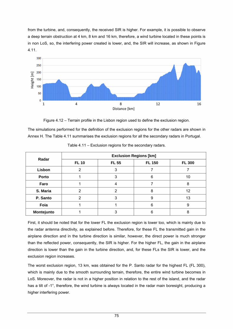
75
from the turbine, and, consequently, the received SIR is higher. For example, it is possible to observe
a deep terrain obstruction at 4 km, 8 km and 16 km, therefore, a wind turbine located in these points is
in non LoS, so, the interfering power created is lower, and, the SIR will increase, as shown in Figure
4.11.
Figure 4.12 – Terrain profile in the Lisbon region used to define the exclusion region.
The simulations performed for the definition of the exclusion regions for the other radars are shown in
Annex H. The Table 4.11 summarises the exclusion regions for all the secondary radars in Portugal.
Table 4.11 – Exclusion regions for the secondary radars.
Radar Exclusion Regions [km]
FL 10 FL 55 FL 150 FL 300
Lisbon 2 3 7 7
Porto 1 3 6 10
Faro 1 4 7 8
S. Maria 2 2 8 12
P. Santo 2 3 9 13
Foia 1 1 6 9
Montejunto 1 3 6 8
First, it should be noted that for the lower FL the exclusion region is lower too, which is mainly due to
the radar antenna directivity, as explained before. Therefore, for these FL the transmitted gain in the
airplane direction and in the turbine direction is similar, however, the direct power is much stronger
than the reflected power, consequently, the SIR is higher. For the higher FL, the gain in the airplane
direction is lower than the gain in the turbine direction, and, for these FLs the SIR is lower, and the
exclusion region increases.
The worst exclusion region, 13 km, was obtained for the P. Santo radar for the highest FL (FL 300),
which is mainly due to the smooth surrounding terrain, therefore, the entire wind turbine becomes in
LoS. Moreover, the radar is not in a higher position in relation to the rest of the island, and the radar
has a tilt of -1°, therefore, the wind turbine is always located in the radar main boresight, producing a
higher interfering power.

76
From the Table 4.11, one defines an exclusion region in [1, 2] km around the radar for an airplane
level of FL 10. For FL 55 the exclusion region increases up to 4 km, for the FL 150 the exclusion
region ranges in [6, 9] km. Finally for the upper FL, it was observed that the maximum values for the
exclusion region that can go up to 13 km.
Moreover, one can conclude that the radar tilt and the position relative to the turbine have a major role
in exclusion regions, especially for the higher FLs. For example, the radar in S. Maria and in P. Santo
are in a higher position relative to the turbines, however, the radar in S. Maria does not have down tilt,
and, consequently the exclusion region is lower than P. Santo.
Using the exclusion regions computed above, and, comparing with the wind turbines locations,
presented in Table 4.2, it is possible to state the following:
The wind turbines located in the Lisbon’s radar vicinity do not affect the secondary radar
correct operation, because all the identified turbines are farther the exclusion region of 7 km
for the worst case, FL 300.
The wind turbines located in the Montejunto’s region, also do not create measurable
interference to the radar in that region.
The P. Santo radar has 3 wind turbines within the exclusion region. The wind turbines are
located at 4.55 km, therefore, they can produce measurable interference to an airplane in
FL 150, and in FL 300.
The S. Maria radar has also 3 wind turbines in their vicinity, located at a distance of 4.95 km.
FL 150 and FL 300 can have a compromised radar correct operation.
The 5 wind turbines in the Foia region are only at 2 km from radar; therefore, they can create
measurable interference to an airplane in FL 150 and FL 300.
The Porto and Faro regions do not have wind turbines in their vicinity, therefore, for future
wind turbine implementations, within the presented exclusion regions, a further analysis must
be performed to assess the impact.

77
Chapter 5
Conclusions 5 Conclusions
This chapter finalises the work, summarising conclusions and pointing out aspects to be developed in
future work.
78
This thesis consists of the assessment of the impact created by wind turbines on radars. The impact is
differentiated for the different types of surveillance radars used by NAV Portugal. A study was
performed for each radar in Portugal mainland, in Azores and in Madeira. After the assessment,
exclusion regions are defined for the radars.
Chapter 2 discusses the basic concepts on which the problem is based. The main aspects referred in
this chapter are: the current surveillance systems existents, the primary and secondary radars working
mode, and the characterisation of wind turbines. The chapter finalises by introducing the influence
created by wind turbines on radars and the problem state of the art.
In Chapter 3, one presents the models used in this study to analyse and quantify the amount of
interference created by the wind turbines on radars. First, one presents the propagation models, as
the radio-horizon distance, the attenuation created by the terrain and by the atmosphere in the radar
signals. One also presents the spherical Earth model used in this study to take the curvature of the
Earth into account. Thereafter, models are presented to characterise the wind turbine from the radar
view point, which are the Radar Cross Section (RCS) and the diffraction theory. Then, the models to
quantify the interference created by the wind turbines on primary and secondary radar are developed.
Finally, Chapter 3 presents the definition of the Flight Routes, used to simulate the airplane path, to
measure the wind turbine impact on different airplane positions.
Chapter 4 starts by presenting the scenarios used in this study, followed by the simulations results.
The simulations were divided into three main interference analyses, which are:
the Doppler Shift created by the wind turbines and the impact on radars;
the impact created by the presence of wind turbines in the Lisbon region on the primary radar;
the impact on the secondary radars in Lisbon, Montejunto, Faro, Foia, S. Maria, and P. Santo.
The main goal of this study is the definition of the exclusion regions around surveillance radars,
therefore, Chapter 4 ends with the methods and the definition of these exclusion regions.
To analyse the Doppler shift impact on a radar, two wind turbine extreme cases were analysed,
namely, 44 m of rotor diameter with a rotation period of 34 RPM and, 100 m of rotor diameter with a
rotation period of 13 RPM.
The maximum speed at the blade edge is 281.88 km/h for the smaller wind turbine, and 244.8 km/h for
the larger. Consequently, the smaller wind turbines, because they spin faster, produce more Doppler
shift, around 1 483 Hz for the primary radar and 569 Hz for the secondary one. The maximum shift is
achieved when the rotor is perpendicular to the radar. When the turbine is facing the radar there are
no changes in frequency. For both cases, 44 m and 100 m of rotor diameter, the frequency deviation
is under the radar tolerance. However, for the PSR operation, and due to the high radial velocity at the
blade edge, the frequency shift produced can be similar to an aircraft, therefore, the MTI can
recognises the wind turbine as a target.
The simulation results of the wind turbine impact on primary radar started by assessing the impact of
different blade materials, different radar operation frequency and different wind turbine orientations on
the scattered energy. The combination of the previous factors that creates the worst result were used

79
to simulate the impact of wind turbines that are in the interfering zone (16 km) around the Lisbon
radar. Moreover, the simulations were divided into the wind turbines that create scattered energy that
is always above the threshold, and into the ones that are only sometimes above the threshold, this
distinction being due to the time-varying model used for the blades RCS. From the simulation results,
it can be concluded that there is not much difference (less than 1 dB) between the models used for
metallic blades and for the dielectric ones. On the other hand, the impact of the radar operation
frequency can lead to differences up to 10 dB, therefore, the radar carrier of 2 840 MHz creates less
scattered energy. For the turbines in the Lisbon region, the maximum radar received power is in
[-37.95, -28.60] dBm, which is a high value, far above the threshold, mainly due to the high values
computed for the RCS which are in [27.67, 36.05] dBsm. These values for the wind turbines RCS are
compliant with the maximum value provided by EUROCONTROL. The usual orientation that leads to a
higher received power is NNW. The terrain attenuation has a major role in the impact created by wind
turbines on a primary radar, because it affects the signal twice, due to the two-way signal path.
The assessment of the impact created by wind turbines on a secondary radar is differentiated from the
up- and downlinks. One has simulated the impact in the received SIR for the radar pointing to the
turbine and for the radar pointing to the airplane; and, as expected, for the first, the SIR is below the
threshold of 10 dB, while, for the second, the SIR is above the threshold, however, the former does
not create interfering problems due to the implementation of ISLS. One has also simulated the impact
of a wind turbine pointing to prevailing winds (NNW), in comparison with it facing the radar; and it can
be concluded that when the wind turbine is facing NNW, the diffraction coefficient is lower than when it
is facing the radar, therefore, the SIR is higher. The impact of different FLs and FRs on the received
SIR also analysed; it can be stated that the higher the FL, the lower the SIR. This fact is mainly due to
the radar antenna vertical diagram, because for the higher FL the gain in the airplane direction is low
and in the wind turbine direction is high, therefore, it will lead to a lower SIR. The worst FRs, due to
the horizontal radiation pattern, are those that are in the same azimuth as the wind turbine. It was
observed that the SIR for the downlink is always lower than for the uplink, which is mainly because in
the downlink the whole turbine is visible, therefore, it creates more interference. Furthermore the
difference in the carrier frequency leads to differences in the received powers. For all scenarios, the
computed SIR was always above the conservative threshold of 20 dB. However, for the critical points
(points where the turbine and the airplane lay in the same azimuth relative to the radar), the simulator
has no resolution to state with any doubts that interfering problems cannot occur. Moreover, the
simulator does not take into account the fading that can affect the signal and originate a decrease in
SIR. The main reasons for simulation results being above the thresholds are as follows:
the radar is very directive, with a horizontal half power beam width of 2.4° and a vertical one of
11°, consequently, when the wind turbine and the airplane are not in the same azimuth the
interference caused by the wind turbine is very low;
the FR report points (VOR positions) are relatively far from the radar, therefore the probability
of having a FR in the same azimuth as the wind farm is relatively low.
The exclusion region for the primary radar was defined using two different methods: assuming flat

80
terrain, or terrain attenuation. For both, one has used the maximum values observed for the wind
turbine RCS and for the maximum received power. The exclusion region for the first method is around
200 km, and for the second method one needs 38.5 dB of terrain attenuation. The radar carrier of
2 840 MHz is the best choice to minimise the impact of the wind turbine scattered energy, and
moreover, leads to higher values of terrain attenuation. For the interfering region (16 km) the scattered
energy is always above the threshold, therefore, it is necessary to have a signal processing to reject
the clutter coming from a wind farm, as implementing software based spectrum filters, or, using
adaptive MTI techniques.
The exclusion region for the secondary radar was obtained by using the simulations for the critical
points, which are the situations where the airplane and the wind turbine lies in the same azimuth.
Therefore, one tested the SIR for different wind turbines distances to the radar and for different FL. It
was observed that the exclusion region is different for each radar, because it depends on the
surrounding terrain, the location, the height and the tilt. An equally exclusion region around the radar
was assumed. Being observed that, for the upper FL, the exclusion region is higher, due to the radar
antenna directivity. The worst exclusion region, 13 km, was obtained for the P. Santo radar for the
highest FL (FL 300), which is mainly due to the smooth surrounding terrain, therefore, the entire wind
turbine becomes in LoS. Moreover, the radar is not in a higher position relative to the rest of the
island, and the radar has a tilt of -1°, therefore, the wind turbine is always located in the radar main
boresight, producing a higher interfering power. One has defined an exclusion region in [1, 2] km
around the radar for an airplane level of FL 10. For FL 55 the exclusion region increases up to 4 km,
for the FL 150 the exclusion region ranges in [6, 9] km. Finally, for the upper FL, the maximum values
for the exclusion region can go up to 13 km. Moreover, one can conclude that the turbines located in
S. Maria, P. Santo and Foia region are within the computed exclusion region for FL 150 and for
FL 300. The wind turbines located in Lisbon, and Montejunto, do not create measurable interference.
This study has also some limitations, and, therefore, some suggestions for future improvements and
work to perform on this subject are given below:
A model to analyse the impact created by the wind turbine nacelle was not considered in this
study, because the shape changes from manufacturer to manufacturer, so, it is impossible to
predict the behaviour on the radar signal.
The results obtained in the simulations need to be compared with real measurements, to
check the validity of the used models.
The results from the simulations of the impact on primary radar give the maximum and the
minimum received powers, however, it is useful to know the average scattered value, in order
to better assess these results.
As previously said, the simulations to assess the impact on a secondary radar do not have
resolution enough to state that the points that fall near the thresholds will not originate
interference problems, due to the airplane path resolution, and to other problems that can
affect the signals, as the fading.

81
Annex A
Building Restricted Areas for
Surveillance Facilities
Annex A. Building Restricted Areas for Surveillance Facilities
This Annex provides the Building Restricted Areas (BRA) description, according with ICAO. BRA are
defined as a volume where buildings have the potential to cause unacceptable interference to the
signal-in-space in the service volume of communication, navigation and surveillance facilities for All
Weather Operations [ICAO09].

82
BRA are defined as a volume where buildings have the potential to cause unacceptable interference
to the signals, in this case is defined as the minimum critical distance, in relation to a surveillance
sensor, where no structure should be placed. The BRA is considered to provide worst case
protection. The cylinder presented in Figure A.1 is referenced to the ground terrain, and the cone is
referenced to a horizontal plane. Where the following parameters present varies depending on the
type of sensor, Table A.1 shows these distances for the surveillance equipment.
is the radius of first cylinder;
is the radius of cone;
is the angle of cone;
is the radius of second cylinder;
is the height of second cylinder.
Figure A.1 – Omni-directional BRA shape, side elevation view (extracted from [ICAO09]).
Table A.1 – Harmonised guidance figures for the omni-directional Surveillance facilities in accordance
with Figure A.1 (extracted from [ICAO09]).
Type of surveillance
facilities [°] [km] [m] Origin of cone
PSR 0.25 15 500 Base of antenna at
ground level
SSR 0.25 15 500 Base of antenna at
ground level

83
Annex B
Recommended SSR Protection
Range
Annex B. Recommended SSR Protection Range
This Annex presents the recommended SSR protection range, used in Chapter 2, to define the
interfering region for the assessment. This recommended range uses the worst case for the radar
parameters, like the ISLS minimum distance to distinguish between the direct and the reflected signal,
and, the minimum distance to avoid bearing errors.

84
The selection of the recommended SSR protection range is based on the assessment of 3 impacts
that a single wind turbine could have on the SSR performance [EURO10]:
Position detection and Mode A/Mode C code detection performance characteristics.
Multiple target reports performance characteristic.
Azimuth accuracy performance characteristic.
SSR interrogations/responses can all be modelled as one-way communication link and probabilities of
signal detection can be derived by from the received signal power, . The received power can be
found by initially determining the power density, , at a range of from a transmitter, as
shown in Figure B.1, radiating a signal with a power of
,
4 (B.1)
The radar’s ability to collect this power and feed it to its receiver is a function of its antenna’s effective
area, , and is therefore given by:
(B.2)
where:
,
(B.3)
Replacing in (B.2) gives:
, ,
4
(B.4)
When this signal is reflected off an object with bi-static radar cross section of σ, e.g. a wind turbine,
rather than received directly, as suggested on Figure B.1, this equation can be modified to:
4 (B.5)
where:
is the transmitted antenna gain in the direction of the wind turbine;
is the received antenna gain in the direction of the wind turbine.
By replacing the power received, , with the threshold of the receiving system, , the distance from the turbine where the reflected signal is likely to be detected is given by:
4 (B.6)

85
Figure B.1 – Direct and reflected signal paths.
If the interrogation signal through main lobe is reflected onto a wind turbine, and the ISLS signal goes
by direct path then, it may happen that when the interrogation arrives, the ISLS has already turned off
the transponder for 35 µs, the path distance travelled by the signal, during this time interval, is:
/ΔΔ2
⇔/ Δ
2⇔
3 10 . 35 102
5250m (B.7)
where:
is the speed of electromagnetic waves in vacuum;
∆ is the distance;
∆ is the time difference.
Any airplane located closer than 5 250 m (half of distance corresponding to 35 μs) will not reply to
reflected interrogations because, in this case, the path difference between the direct and the reflected
signal will always be lower than 35 µs.
When the aircraft transponder is located further than 5 250 m from the wind turbine, the minimum
power received by the transponder from a reflected interrogation can be calculated and can be
compared with the transponder minimum receiver threshold (smaller specified value -77 dBm
[ICAO07b]). Therefore, the minimum distance between the SSR and the wind turbine is estimated as
15698 m, calculated using (B.6) assuming the values [EURO10]:
Table B.1 – Values assumed to compute de SSR recommended range (extracted from [EURO10]).
-77 dBm
2 KW
35 dBsm
27 dBi
0 dBi
5 250 m
1 030 MHz
Therefore when the wind turbine is 16 km away from the SSR, if the airplane is located closer than 5
250 m from the wind turbine, the transponder will not reply to reflected interrogations because of ISLS
implementation and when further than 5 250 m, the power of the reflected interrogation will be below
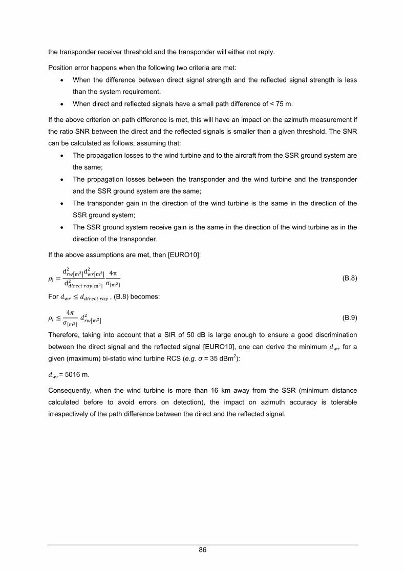
86
the transponder receiver threshold and the transponder will either not reply.
Position error happens when the following two criteria are met:
When the difference between direct signal strength and the reflected signal strength is less
than the system requirement.
When direct and reflected signals have a small path difference of < 75 m.
If the above criterion on path difference is met, this will have an impact on the azimuth measurement if
the ratio SNR between the direct and the reflected signals is smaller than a given threshold. The SNR
can be calculated as follows, assuming that:
The propagation losses to the wind turbine and to the aircraft from the SSR ground system are
the same;
The propagation losses between the transponder and the wind turbine and the transponder
and the SSR ground system are the same;
The transponder gain in the direction of the wind turbine is the same in the direction of the
SSR ground system;
The SSR ground system receive gain is the same in the direction of the wind turbine as in the
direction of the transponder.
If the above assumptions are met, then [EURO10]:
d d
d
4πσ
(B.8)
For , (B.8) becomes:
4 (B.9)
Therefore, taking into account that a SIR of 50 dB is large enough to ensure a good discrimination
between the direct signal and the reflected signal [EURO10], one can derive the minimum for a
given (maximum) bi-static wind turbine RCS (e.g. σ = 35 dBm2):
= 5016 m.
Consequently, when the wind turbine is more than 16 km away from the SSR (minimum distance
calculated before to avoid errors on detection), the impact on azimuth accuracy is tolerable
irrespectively of the path difference between the direct and the reflected signal.

87
Annex C
Shadow Region Assessment
Annex C. Shadow Region Assessment
If a wind turbine lies in the radar LoS it generates a shadow region behind it that could degrade the
radar performance. The possibility therefore exists that desired targets in the shadow zone could be
lost due to the reduction in field strength of the radar signal [LCST08]. This Annex analyses the
amount of shadow created by the wind turbine.

88
The general shape of the shadow is a three-dimensional wedge [LCST08], therefore, to make the
complete assessment must be done the calculation of the shadow length, height and width.
The shadow length correspond to the maximum distance that the aircraft is able to detect the reflected
signal. This protection range is calculated based on the transponder receive threshold that beyond
this distance the reflected interrogation signal would dissipate to a level that is less than the
sensitivity of the transponder [Yun11]. The Equation (B.6) gives the maximum distance:
, ,
4 (C.1)
The shadow height is calculated by considering the geometry of the wind turbine and the transmitter,
as shown in Figure C.1, taking into account the maximum height of the turbine, the Earth curvature,
the Earth radius ( ) with the corrective factor k of 4/3. Figure C.1 shows the shadow geometry to aid
on shadow height calculation.
Figure C.1 – Wind turbine shadow geometry (adapted from [EURO10]).
The height of the shadow zone can be calculated taking into account the following equations, and
using the symbols expressed in Figure C.1 [EURO10]:
(C.2)
(C.3)
2 cos (C.4)
where:
(C.5)
° (C.6)

89
(C.7)
° ° (C.8)
° ′ (C.9)
°
° (C.10)
The height of the shadow zone can be calculated as follows:
(C.11)
where:
is the wind turbine shadow height.
A typical cross-range section of the shadow effect is shown in Figure C.2, where a reflection from a
metallic object is assumed, hence the direct and reflected signals will be anti-phase [EURO10]. It is
also shown the power fluctuation in function of the distance to the wind turbine as well as two
important points, the point A which represents the deepest shadow and the point B which represents
the maximum power (meaning a week shadow region) [EURO10].
Figure C.2 – Diagram of a cross-section of a shadow (extracted from [EURO10]).
Figure C.2 shows that at point A the path difference between direct and reflected signal is zero and
the signals combine in a destructive way, causing the deepest shadow. At point B the path difference
is λ/2 and the signals combine constructively to give a maxima [EURO10]. Moreover, successive
maxima are odd multiples of λ/2, where path difference is given by (2n+1) /2, and n is a positive
integer. Figure C.2 also shows that the maxima gets weaker, this is because the interfering signal is
weaker at larger angles off the forward-scatter direction [EURO10].
A conservative estimate of the shadow width is the locus of points formed by point B as a function of
down-range; the geometry is shown in Figure C.3. The path difference, Δ, between the direct and
reflected signals at the receiver is given by [EURO10]:
Δ (C.12)
where:
is the reflected path distance.

90
Figure C.3 – Path difference geometry for shadow width calculation (extracted from [EURO10]).
The width of shadow at a distance beyond the turbine is found by setting the path difference equal to
λ/2 and solving for half-width, [EURO10]:
2 (C.13)
2 . (C.14)
for ≪ .
The impact on the one-way transmission of field strength to a point in the shadow depends, as seen
above, one the distances between the transmitter, the turbine, and the point . The ratio of the power
received via the direct path has to be compared to the power received via the indirect path. Combining
(B.1) and (B.5), it comes [EURO10]:
, , 4
(C.15)
By inverting (C.15), one gets the ratio between the direct and reflected signals behind the turbine:
, , 4 (C.16)
For a point A, directly behind the turbine, the following relationship can be used [EURO10]:
, (C.17)
, (C.18)
(C.19)
4 (C.20)
Replacing the above assumptions in (C.16), it gives [EURO10]:
(C.21)
Using the relationship between field strength and power loss due to shadow zone ( ), one gets:
1 1 (C.22)

91
In dB, it becomes:
40 log 1 (C.23)
where:
is the attenuation in the shadow region.

92

93
Annex D
3D Radiation Pattern
Annex D. 3D Radiation Pattern This Annex provides the algorithm adopted to compute the radar gain in a certain direction, because
ATC radars radiation patterns are very directive, therefore it is crucial to take into account the
variations in the gain for the received power via direct and reflected paths. The gain in a certain
direction is computed using an extrapolation method of the horizontal and vertical radiation patterns.

94
The radar antennas are usually very directive, as such, it is necessary to account for the changes in its
gain to correctly compute the received power in any direction. Therefore, it is necessary to determine
the angular difference in the horizontal and vertical planes between the desired direction and the
direction of maximum radiation of the antenna.
Figure D.1 represents the geometry of the problem presenting the horizontal and vertical planes of the
radiation pattern, and the point P. To calculate the gain in the direction of point P is necessary to know
the value of and in 3D radiation pattern, therefore, it is necessary to know the value of the angles
corresponding to the azimuth and elevation of a given point in relation to the direction of maximum
gain [ClFe98].
Figure D.1 – Geometry of the extrapolation method to obtain the 3D radiation pattern (extracted from
[ClFe98]).
The antenna manufacturers usually provide the radiation patterns in the horizontal and vertical planes,
the respective half power beam widths, and the maximum gain. Therefore, the gain at each point in
the 3D diagram is extrapolated from the points which are closest, in the radiation patterns, whose gain
is known [ClFe98]. For each point P, three of the four closest points are in the vertical plane, and their
gains are , and , while , and are the angular distances from these points to P,
respectively. In the horizontal plane, point P has a gain of and its angular distance is [ClFe98].
It is assumed that the horizontal and vertical radiation patterns are known, defined as and
respectively, and with ∈ /2, /2 and ∈ 0, /2 [OlCa02]. Therefore, the gain at point P in any
direction is given by the following extrapolation method [OlCa02]:
,
(D.1)
where:
, , , are defined in Figure D.1;
0 or /2 ;
;

95
.
When or are zero, , is directly obtained by or , respectively [ClFe98].
As shown in Figure D.2, the radar’s manufactures in reality do not provide the antenna vertical
radiation pattern, instead of that, they provide the vertical coverage diagram. This type of diagram
shows the radar length coverage, in NM, in function of the height coverage, in Kft. Due to the high
coverage distance, the curvature of the Earth is taken into account, as shown in Figure D.2, the
curved lines representing the coverage variation distortion.
However, in this study, the distances between the radar and the airplane do not go beyond 100 km
(nearly 50 NM), and, as shown in Figure D.2, for these distances, the Earth curvature impact on
coverage diagram can be neglected. Then, a linear proportion between the length coverage and the
height coverage can be used, in order to get the normalised gain in relation to the maximum.
Figure D.2 – MSSR uplink vertical coverage diagram (extracted from [NAV13c]).
To convert the coverage diagram into a radiation pattern, some points were taken from the first one.
Then, all the points coordinates (Kft, NM) were converted to S.I. units, in order to have the same units
for the length and the height. Thereafter, the distance between each point and the origin was
measured, and then, their angle in relation to ground reference was computed. The normalised gain
was computed by dividing the distance of each point by the distance of the maximum coverage point
(near 8º in the coverage diagram of Figure D.2).
Figure D.3 illustrates the radiation pattern resulting from the conversion, showing the normalised gain
for different elevation angles. The antenna half power beamwidth is consistent with the information
provided by manufacturer. The red lines in Figure D.3 representing the elevation angles, in relation to
the radar, while, blue line, represent the horizontal radiation patter.

96
Figure D.3 – MSSR uplink vertical radiation pattern.
The horizontal radiation pattern was provided by NAV, therefore, it was just necessary to take some
points in order to have the relative gain in function of the azimuthal angle. Figure D.4 shows the
resulting radiation pattern.
Figure D.4 – MSSR horizontal radiation pattern.
Note that, as above described, both radiation patterns are discrete, therefore, the number of available
points is limited. To apply (D.1), in order to have the 3D radiation pattern, the points whose angles
were the most approximated to the real values were chosen, and the corresponding gains were used.
To obtain both radiation diagrams for the primary radar the same process above described was done,
the resulting diagrams are shown in Figure D.5 and Figure D.6.

97
Figure D.5 – PSR vertical radiation pattern.
Figure D.6 – PSR horizontal radiation pattern.

98

99
Annex E
Wind Turbines Coordinates
Annex E. Wind Turbines Coordinates This Annex provides the geographical coordinates of the wind turbines that fall into the interference
region, and, therefore being part of the scenarios for analysis.

100
Table E.1 shows the geographical coordinates for all the wind turbines identified in the radars
interfering region. The first column of Table E.1 shows the corresponding radar, and the column in the
middle shows the wind farm which the turbine belongs.
Table E.1 – Wind Turbines geographical coordinates.
Radar Wind Farm WT coordinates [degrees]
Foia Radar Madrinha
37.30699,-8.62271
37.30675,-8.62075
37.30671,-8.61875
37.30694,-8.61686
37.30954,-8.62730
P. Santo Radar Cabeço do Carvalho
33.05867,-16.3634
33.0584,-16.3650
33.0584,-16.36500
S. Maria Radar Figueiral
36.94916,-25.1291
36.94865,-25.1310
36.94806,-25.1333
Lisbon Radar
Almargem
38.84415,-9.26662
38.84138,-9.26744
38.83927,-9.26768
Bolores
38.86336,-9.23018
38.86157,-9.22917
38.85907,-9.22708
38.86075,-9.22214
Sardinha
38.87141,-9.22018
38.87458,-9.22520
38.88018,-9.22301
38.87969,-9.22575
38.88292,-9.21237
38.88353,-9.20969
38.88693,-9.21382
38.86292,-9.23556
38.86149,-9.23836
38.85989,-9.24055
38.857893,-9.2431
38.856241,-9.2455

101
Table E.1 (Cont.) – Wind Turbines geographical coordinates.
38.88031,-9.21783
Valérios 38.8882,-9.20089
Fanhões
38.89639,-9.15319
38.89601,-9.14991
38.89485,-9.14744
38.89073,-9.14955
38.88980,-9.14503
38.8855,-9.139601
38.88079,-9.14288
38.88022,-9.14472
38.87745,-9.14557
V. F. Xira
38.88891,-9.11900
38.89127,-9.11789
38.8919,-9.114935
38.89282,-9.11206
Montejunto Radar
Alto da Folgorosa
39.11939,-9.14937
39.12611,-9.13964
39.12905,-9.13787
39.13211,-9.13413
39.13409,-9.13109
39.13545,-9.12813
39.14042,-9.12526
39.14055,-9.12208
39.14110,-9.11891
Joguinho
39.12067,-9.14541
39.12147,-9.14260
39.12398,-9.14158
39.1113,-9.162117
39.10987,-9.17037
39.10769,-9.16715
39.10447,-9.16293
39.10225,-9.16560
39.10194,-9.16900
39.1000,-9.170668
39.09772,-9.17097
39.09232,-9.17347
39.09075,-9.17662
39.10986,-9.1704

102
Table E.1 (Cont.) – Wind Turbines geographical coordinates.
Achada
39.10862,-9.196314
39.10865,-9.193664
39.10843,-9.190799
Caldas
39.29724,-9.010648
39.29578,-9.013851
39.294554,-9.01069
39.29437,-9.015329
39.29430,-9.017952
Serra de Todo-o-mundo
39.29313,-9.021868
39.29283,-9.025076
39.29267,-9.027911
39.29012,-9.030475
39.28830,-9.032535

103
Annex F
NAV Portugal, E.P.E
Surveillance Systems
Annex F. NAV Portugal, E.P.E Surveillance Systems
This Annex provides the description of the NAV surveillance radars main characteristics. The radars
presented in this Annex are used in this Thesis to analyse the impact caused by the wind turbines on
them.

104
(Confidential Annex)

105
Annex G
Flight Routes
Annex G. Flight Routes This Annex provides information about the Flight Routes used in this Thesis to analyse the impact
caused by the wind turbines in aeronautical radars. The Flight Routes represents the airplane most
probable path in the airspace.
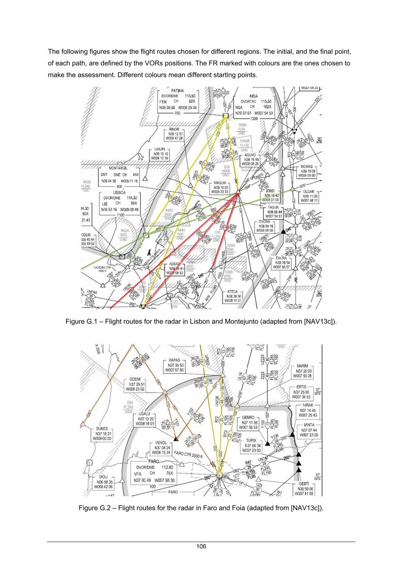
106
The following figures show the flight routes chosen for different regions. The initial, and the final point,
of each path, are defined by the VORs positions. The FR marked with colours are the ones chosen to
make the assessment. Different colours mean different starting points.
Figure G.1 – Flight routes for the radar in Lisbon and Montejunto (adapted from [NAV13c]).
Figure G.2 – Flight routes for the radar in Faro and Foia (adapted from [NAV13c]).

107
Figure G.3 – Flight routes for the radar in S. Maria (adapted from [NAV13c]).
Figure G.4 – Flight routes for the radar in P. Santo (adapted from [NAV13c]).
Figure G.5 – Flight routes for the radar in Porto (adapted from [NAV13c]).


109
Annex H
Results for Secondary Radar
Exclusion Region
Annex H. Results for Secondary Radar Exclusion Region
This Annex provides the results from the simulations for the definition of the exclusion regions for the
secondary radars that belongs to NAV Portugal. The simulations were made for different airplanes
flight levels. in order to assess their impact in the exclusion regions.

110
The following Figures show the simulation results to create the exclusion regions, as defined in Sub-
section 4.5.2. The Figures shows the received SIR, for different airplane FL, and for different wind
turbine locations. The black line represents the defined threshold, 10 dB. The exclusion regions are
dependent on surrounding terrain, tilt, and height; therefore, the analysis must be performed to each
radar. To define the exclusion region, the values for the higher wind turbine presented in Table 4.2
were used. The first analysis is for a wind turbine at 1 km from the radar, and the distance increases 1
km progressively, up to 16 km. For the test, just one wind turbine was considered.
Figure H.1 – SIR for a wind turbine at different distances around S. Maria radar.
Figure H.2 – SIR for a wind turbine at different distances around P. Santo radar.
‐10
‐5
0
5
10
15
20
25
30
35
40
1 2 3 4 5 6 7 8 9 10 11 12 13 14 15 16
SIR
[dB
]
Distance [km]
FL 10
FL 55
FL 150
FL 300
SIR minimum
‐10
‐5
0
5
10
15
20
25
30
35
1 2 3 4 5 6 7 8 9 10 11 12 13 14 15 16
SIR
[dB
]
Distance [km]
FL 10
FL 55
FL 150
FL 300
SIR minimum

111
Figure H.3 – SIR for a wind turbine at different distances around Faro radar.
Figure H.4 – SIR for a wind turbine at different distances around Foia radar.
Figure H.5 – SIR for a wind turbine at different distances around Montejunto radar.
‐5
0
5
10
15
20
25
30
35
1 2 3 4 5 6 7 8 9 10 11 12 13 14 15 16
SIR
[dB
]
Distance [km]
FL 10
FL 55
FL 150
FL 300
SIR minimum
‐5
0
5
10
15
20
25
30
35
40
1 2 3 4 5 6 7 8 9 10 11 12 13 14 15 16
SIR
[dB
]
Distance [km]
FL 10
FL 55
FL 150
FL 300
SIR minimum
‐5
0
5
10
15
20
25
30
35
40
1 2 3 4 5 6 7 8 9 10 11 12 13 14 15 16
SIR
[dB
]
Distance [km]
FL 10
FL 55
FL 150
FL 300
SIR minimum

112
Figure H.6 – SIR for a wind turbine at different distances around Porto radar.
‐5
0
5
10
15
20
25
30
35
40
1 2 3 4 5 6 7 8 9 10 11 12 13 14 15 16
SIR
[dB
]
Distance [km]
FL 10
FL 55
FL 150
FL 300
SIR minimum

113
References
References [ABB11] ABB, Wind power plants, Technical Application Papers No.13, Bergamo, Italy, 2011,
(http://www05.abb.com/global/scot/scot209.nsf/veritydisplay/92faf0c1913f5651c1257937
002f88e8/$file/1sdc007112g0201.pdf).
[AIRN12] http://air-nav-srf.blogspot.pt/2012/05/secondary-surveillance-radar-ssr.html, Nov. 2012.
[Akka09] Akkaşlı,C., Methods for Path loss Prediction, Reports from MSI, School of Mathematics
and Systems Engineering, Report 09067, Växjö University, Växjö, Sweden, Oct. 2009.
[Alex04] Alexander,J., “Loxodromes: A Rhumb Way to Go”, Mathematics Magazine, Vol. 77, No 5,
Dec. 2004, pp.349-356.
[Alle04] Allen,C., Radar Pulse Compression, Presentation, Information and Telecommunication
Technology Center, University of Kansas, Laurence, KS, USA, 2004,
(http://www.ittc.ku.edu/workshops/Summer2004Lectures/Radar_Pulse_Compression.pdf)
[Amat09] Amato,N.J., Modeling and Simulation Architecture for studying Doppler-Based Radar with
Complex Environments, M.Sc. Thesis, Air Force Institute of Technologic, Ohio, OH, USA,
2009.
[ATC12] http://www.atc-network.com/atc-industry/nav-portugal, Dec. 2012.
[ATCS12] http://atcsl.tripod.com/radar_theory.htm, Nov. 2012.
[Bake11] Baker,C.,J., Aviation Radar Systems, Lecture notes, OHIO State University, Columbus,
OH, USA, 2011 (http://esl.eng.ohio-
state.edu/~cbaker/cb_files/classes/ece714/lectures/13.%20Aviation%20Radar%20Syste
ms_2011.pdf).
[BGHL10] Baud,O., Gomord,P., Honoré,N., Lawrence,P., Ostorero,L., Paupiah,S. and Taupin,O.,
Air Traffic Control Tracking Systems Performance Impacts with New Surveillance
Technology Sensors, Aerospace Technologies Advancements, InTech, Vienna, Austria,
2010 (http://www.intechopen.com/books/aerospace-technologies-advancements/air-
traffic-controltracking-systems-performance-impacts-with-new-surveillance-technology-
sensors).
[CAA12] Civil Aviation Authority, CAP 670 ATS Safety Requirements – Amendment 13, Safety
Regulation Group, London, UK, Nov. 2012 (http://www.caa.co.uk/docs/2532/20121119
CAP670Amdt013ExternalConsultationDocument.pdf).
[CAA13] Civil Aviation Authority, Policy and Guidelines on Wind Turbines, Stationary Office, Fifth

114
Edition, London, UK, June 2013 (www.caa.co.uk/publications).
[Cast10] Castro,R.M.G., Introduction to Wind Energy (in Portuguese), Lecture Notes, Instituto
Superior Técnico, Lisbon, Portugal, 2010.
[ChRa12] http://boonton.com/resource-library/articles/characterising-radar, Nov. 2012.
[ClFe98] Claro,A. and Ferreira,J., Propagation Models Evaluation for Non-Regular Urban GSM
900 Micro Cells (in Portuguese), Dipl. Thesis, IST-TUL, Lisbon, Portugal, Sep. 1998.
[Corr12] Correia,L.M., Mobile Communications Systems Lecture Notes, IST-TUL, Lisbon,
Portugal, Feb. 2012.
[DeDe06] Department of Defence, The Effect of Windmill Farms On Military Readiness , Report to
the Congressional, Office of the Director of Defence Research and Engineering, Arlington
County, Virginia, USA, 2006 (http://www.defense.gov/pubs/pdfs/WindFarmReport.pdf).
[DTI02] Department of Trade and Industry, Wind Energy and Aviation Interests-Interim guidelines,
Wind Energy, Defence & Civil Aviation Interests Working Group, London, UK, 2002
(http://www.apere.org/docnum/recherche/view_docnum.php?doc_filename=doc1288_avi
ation.fiche115.pdf&num_doc=1288).
[EETI12] http://www.eetimes.com/design/military-aerospace-design/4398289/Understanding-
Mode-S-technology-, Nov. 2012.
[Elet13] www.elettra2000.it/vdegliesposti/Esercizi Propagazione e Pianificazione LM/ExA2.pdf,
May 2013.
[ENEG11] Wind farms in Portugal (in Portuguese), Public report, INEGI – Instituto de Engenharia
Mecânica e Gestão Industrial & APREN – associação de energias renováveis, Porto,
Portugal, Dec. 2011
(http://e2p.inegi.up.pt/relatorios/Portugal_Parques_Eolicos_201112.pdf).
[Esqu12] http://www.esquerda.net/dossier/protocolo-de-quioto-portugal-o-pior-desempenho-da-
uni%C3%A3o-europeia, Dec. 2012.
[EURO08] Eurocae, Minumim Operational Performance Specifications for Secondary Surveillance
Radar Mode S Transponders, The European Organisation for Civil Aviation Equipment,
Paris, France, Jan. 2008 (http://adsb.tc.faa.gov/SC209_Meetings/WG1_Mtg06-2008-
0414/ModeS-WP06-07-ED73B%20v-h%20Edited%20with%20changes%20accepted
%2010MAR08.pdf).
[EURO10] EUROCONTROL, Guidelines on How to Assess the Potential Impact of Wind Turbines
on Surveillance Sensors, European Organisation for the Safety of Air Navigation,
EUROCONTROL-GUID-0130, Brussels, Belgium, May 2010.
[EURO12a] http://www.eurocontrol.int/msa/public/standard_page/modes_tech_overview.html, Nov.
2012.
[EURO12b] EUROCONTROL, EUROCONTROL Specefications for ATM Surveillance System

115
Performance, EUROCONTROL-SPEC-0147, European Organisation for the Safety of Air
Navigation, Brussels, Belgium, Mar. 2012.
[EURO97] EUROCONTROL, Radar Surveillance in En-Route Airspace and Major Terminal Areas,
SUR.ET1.ST01.1000-STD-01-01, European Organisation for the Safety of Air Navigation,
Brussels, Belgium, Mar. 1997.
[FasR12] http://www.fas.org/man/dod-101/navy/docs/es310/radarsys/radarsys.htm, Nov. 2012.
[FNM09] Frye,A., Neumann C. and Muller A., The compatibility of Wind Turbines with Radars
Annual Report 2008, Report No. 83137677, EADS Deutschland GmbH, Ulm, Germany,
July 2009.
[GREE12] http://www.greenrhinoenergy.com/renewable/wind/wind_technology.php, Nov. 2012.
[Grev07] Greving,G., “Wind Turbines and Radar – The Radar Cross Section RCS a Useful Figure
for Safeguarding?”, in Proc. of International Radar Symposium 2007, Cologne, Germany,
Sep. 2007.
[Hawk09] Hawk,S., Impact Study of 130 Offshore Wind Turbines in Nantucket Sound, Engineering
Services, AJW-W15B, FAA, WSA, USA, Mar. 2009.
[ICAO07a] ICAO, Guidance Material on Comparison of Surveillance Technologies, Montreal,
Quebec, Canada, Sep. 2007 (http://www.icao.int/APAC/Documents/edocs/cns/
gmst_technology.pdf).
[ICAO07b] ICAO, Surveillance Radar and Collision Avoidance Systems, Aeronautical
Telecommunications, Annex 10 Vol. IV to the Convention on International Civil Aviation
Fourth Edition, July 2007.
[ICAO09] International Civil Aviation Organisation, European Guidance Material ON Managing
Building Restricted Areas, European and North Atlantic Office of ICAO, ICAO EUR DOC
015, Neuilly-sur-Seine, France, Sep. 2009.
[IMAG13] http://imageshack.us/photo/my-images/184/lpfirglobalfg2.jpg/, Jan. 2013.
[Indr09a] Indra, Primary Surveillance Radar, Datasheet, Madrid, Spain, 2009,
(www.indracompany.com).
[Indr09b] Indra, Monopulse Secondary Surveillance Mode S Radar, Datasheet, Madrid, Spain, 2009 (www.indracompany.com/sites/default/files/11%20MSSR%20Mode%20S%20Brochure%20V1%2002-2009%20eng_0.pdf).
[Java13] https://developers.google.com/maps/documentation/javascript/, Sep. 2013.
[JeTo12] Jenn,D. and Ton,C., “Wind Turbine Radar Cross Section”, Hindawi International Journal
of Antennas and Propagation, Vol. 2012, Dec. 2012.
[Kell62] Keller,J.B.. “Geometrical Theory of Diffraction”, Journal of the Optical Society of America,
Vol. 52, No. 2, Feb. 1962, pp.116-130.

116
[Kenn12] Kennedy,A.D., Evolution of the Surveillance Infrastructure, Surveillance Infrastructure
Rationalisation Project, Deliverable ID D09-002, EUROCONTROL, Brussels, Belgium,
Apr. 2012.
[Koks08] Koks,D., Using Rotations to Build Aerospace Coordinate Systems, Electronic Warfare
and Radar Division Systems Sciences Laboratory, DSTO-TN-.640, Departement of
Defence of the Australian Government, Edinburgh, Australia, Aug. 2008
(http://www.dtic.mil/cgi-bin/GetTRDoc?AD=ADA484864).
[LCST08] Lemmon,J.J., Carrol,J.E., Sanders,F.H. and Turner,D., Assessment of Effects of Wind
Turbines on ATC radars, U.S. Department of Commerce, Washington, D.C., USA, July
2008.
[Leag13] http://leagueofextraordinarytechnicians.wikispaces.com/Mode+C+Transponder+-
+Testing, Sep. 2013.
[Made10] Madeira,V., Wind Farms servitude (in Portuguese), Internal Report, NAV, Lisbon,
Portugal, Jan. 2010.
[MatL13] Matlab R2013a Documentation, Documentation ,The Mathworks Inc., Natick, MA, US,
2011 (http://www.mathworks.com/).
[MiCh10] Mishra,K. and Chandrasekar,V., “Signal Analysis and Modeling of Wind Turbine Cluter in
Weather Radars”, in Proc. of IEEE International Geoscience and Remote Sensing
Symposium, Hawaii, USA, July 2010.
[MoSe03] Moir,I. and Seabridge,A., Civil Avionics Systems, AIAA Education Series, USA, 2003.
[NAV07] NAV Portugal, Radar Services and Procedures, ENR 1.6 – 1, NAV Portugal E.P.E,
Lisbon, Portugal, Nov. 2007.
[NAV11] NAV, Rules and Procedures, Lisbon, Portugal 2011,
(www.nav.pt/ais/VFRs/Rules%20and%20Procedures.pdf).
[NAV12] NAV Portugal, Parameters of Radar Stations used in Lisbon FIR (in Portuguese), NAV
Portugal E.P.E., Lisbon, Portugal, Dec. 2012.
[NAV13a] http://www.nav.pt/default.aspx?CSeccao=5, Jan. 2013.
[NAV13b] http://www.nav.pt/ais/cd/2013-07-26/html/eAIP/LP-ENR-6-en-PT.html, May 2013
[NAV13c] NAV Portugal, Private Communications, 2013.
[OlCa02] Oliveira,C. and Carpinteiro,G., Impact of the localisation of GSM and UMTS Base Station
Antennas on the Human Exposure to Electromagnetic Radiation (in Portuguese), Dipl.
Thesis, IST-TUL, Lisbon, Portugal, Sep. 2002.
[OrDr86] Orlando,A.V. and Drouilhet,P.R., Mode S Beacon System: Functional Description, Project
Report, Massachusetts Institute of Technology, Cambridge, Massachusetts, USA, 1986
(http://extweb.ll.mit.edu/mission/aviation/publications/publication-files/atc-

117
reports/Orlando_1986_ATC-42d_WW-15318.pdf).
[Orla89] Orlando,A.V., “The Mode S Beacon Radar System”, The Lincoln Laboratory Journal, Vol.
2, No.3, 1989, pp. 345-362.
[Peat08] Peaty,A., Study of Low Power SSR transponder Link Margins, QINETIQ,
QINETIQ/07/03229/1.0, UK, Jan. 2008.
[Pelm05] Pelmoine,C., Present use and perspective for civil primary surveillance radar in Europe,
EUROCONTROL, Brussels, Belgium 2005, (http://www.itu.int/dms_pub /itur/oth/
0A/0E/R0A0E0000730001PPTE.ppt).
[Pere11] Pereira,E., NAV-CNS-ATM FAB SW data compilation, FAB SW, Navegação Aérea de
Portugal – NAV Portugal, E.P.E. DETPRO – Direcção de Estudos Técnicos e Projectos,
Lisbon, Portugal, June 2012.
[Pint11] Pinto,J.V., Assessment and Design of Multilateration Telecommunication Systems
installed in NAV Portugal, M.Sc. Thesis, Instituto Superior Técnico, Lisboa, Portugal,
2011.
[Poup03] Poupart,G.J., Wind Farms Impact on Radar Aviation Interests, Internal Report, QinetiQ,
Farnborough, Hampshire, UK, Sep. 2003.
[Poup06] Poupart,G.J., Assessment of the impact of proposed Creed wind turbine on the Sandwick
SSR radar, QINETIQ/06/02120/1.1, Hampshire, UK, Oct. 2006.
[Rada12] http://www.radartutorial.eu/, Nov. 2012.
[RaLe12] http://business.auburn.edu/~rgg0002/lessons/radar.htm, Nov. 2012.
[Rash07] Rashid,L., “RCS and Radar Propagation Near Offshore Wind Farms”, in Proc. of IEEE
Antennas and Propagation Society International Symposium, Hawaii, USA, June 2007.
[Rayt04] Raytheon, Raytheon’s ASR-23SS series L-Band solid-state primary surveillance radar,
Datasheet, Waterloo, Ontario, Canada, 2004, (www.raytheon.com/cnsatm).
[Rayt04a] Raytheon, Raytheon’s ASR-23SS series L-Band solid-state primary surveillance radar,
Datasheet, Waterloo, Ontario, Canada, 2004, (www.raytheon.com/cnsatm).
[Rayt04b] Raytheon, Raytheon’s ASR-10SS Mk2 series S-Band solid-state primary surveillance
radar, Datasheet, Waterloo, Ontario, Canada, 2004, (www.raytheon.com/cnsatm).
[Rees09] Rees,M., Surveillance strategy, EUROCONTROL, Brussels, Belgium, 2009,
(http://www.enri.go.jp/eiwac/2009/ppts/TheEUROCONTROLSurveillanceStrategy.pdf).
[Ridd05] Riddols,R.J., Effects of Wind Turbines on High Frequency Surface Wave Radar,
Technical memorandum, Defence R&D Canada, Ottawa, Canada, Dec. 2005
(http://cradpdf.drdc-rddc.gc.ca/PDFS/unc49/p525535.pdf).
[Rodr07] Rodrigues,A., Wind Farms in Portugal, INEGI – Instituto de Engenharia Mecânica e
Gestão Industrial, Mar. 2007, (http://www.inegi.up.pt/publicacoes/outras/Wind_Farms_

118
Portugal_Mar 07.pdf).
[Rodr09] Rodrigues,M.A.S., Comunication Systems for the Desert Islands (in Portuguese), M.Sc
Thesis, University of Madeira, Funchal, Portugal, Nov. 2009.
[Sang12] Sanguino,J.E., Navigation Systems Lecture Notes, IST-TUL, Lisbon, Portugal, 2012.
[Secu12] http://www.airport-int.com/article/eurocontrol-takes-action.html, Dec. 2012.
[SSR12] http://www.nec.com/en/global/solutions/cns-atm/surveillance/ssr.html, Nov. 2012.
[STEV90] Stevens,M.C., “Surveillance in the Mode S Era”, in Proc. of CAA/IEE Symposium on
ATC, London, UK, Mar. 1990.
[TLC06] Trappeniers,D., Lil,E.V., Capelle,A.V., “Effects of Objects With moving parts like wind
turbines on maritime RF safety and navigational systems” in Proc. of European
Conference on Antennas and Propagation, Nice, France, Nov. 2006.
[TRAI12] https://trainingzone.eurocontrol.int/ATMTraining/PreCourse/SUR/ADS/Taste%20the%
20Course/32501.10.32657.85.28713/Default.html, Nov. 2012.
[Wind12] http://www.wwindea.org/technology/ch01/en/1_2.html, Nov. 2012.
[Wind13] http://pt.windfinder.com/windstats/windstatistic_lisboa.htm, June 2013.
[WPE12] http://www.windpowerengineering.com/construction/installation/modular-towers-and-the-
quest-for-stronger-wind/, Nov. 2012.
[Yun11] Yun,S., Impact of Riviera wind farm on monopulse surveillance radar at Kingsville naval
air station, ATDI internal report, contract No. N68836-10-P-3103, Paris, France, 2011.