fire & fuels management

Assessment of Fire Effects Based on ForestInventory and Analysis Data and aLong-Term Fire Mapping Data SetJohn D. Shaw, Sara A. Goeking, James Menlove, andCharles E. Werstak Jr.

Integration of Forest Inventory and Analysis (FIA) plot data with Monitoring Trends in Burn Severity (MTBS) datacan provide new information about fire effects on forests. This integration allowed broad-scale assessment ofthe cover types burned in large fires, the relationship between prefire stand conditions and fire severity, andpostfire stand conditions. Of the 42.5 million acres burned in eight Interior West states since 1984, 41.4% wasforestland. Forest types with the most burned acreage were ponderosa pine, lodgepole pine, and Douglas-fir.Nearly 35% of plots had no live basal area of trees �5 in. diameter remaining postfire, but 32% of plots hadgreater than 40 ft2/ac of residual live basal area. Residual basal area appeared to decline slightly with timesince fire, suggesting low mortality rates among survivor trees. Seedlings appeared to reach peak density 5–10years postfire, and sapling density increased monotonically for at least 25 years postfire. Data from remeasuredFIA plots indicate that the highest MTBS severity class is related to high prefire basal area. At a regional scale,MTBS severity classes represent significantly different levels of mean live basal area reductions, ranging from4% for areas of very low fire severity to 89% for high-severity areas. Severity classes are less distinguishablefor individual forest-type groups.

Keywords: forest monitoring, wildfire, fire severity, Monitoring Trends in Burn Severity (MTBS), ForestInventory and Analysis (FIA), regeneration

W ildland fire is arguably the mostimportant forest-related topicin the western United States to-

day. Other disturbances, such as insect anddisease outbreaks, may affect much larger ar-eas than fire in a given year, but the urgencyto protect lives, property, and natural re-sources from fire requires immediate andlarge expenditures. The average annual costof fire suppression now exceeds $1.3 billion

(US Department of Agriculture [USDA]Forest Service 2014). Although suppressioncosts and their impact on the budget of theUSDA Forest Service are usually high-lighted, many other costs can be includedin the calculation of the “true cost” ofwildfire (Western Forestry Leadership Co-alition 2010). Such analyses take into ac-count factors such as direct costs (e.g.,damage to private property and utilities),

indirect costs (e.g., loss of business and taxrevenue), rehabilitation costs, and othercosts, which include adverse health effects,loss of scenic values, and loss of ecosystemservices (Western Forest Leadership Co-alition 2010).

One component that is not well quan-tified is the direct effect on the forest re-source itself. For example, in the estimates oftotal burned area reported annually by theNational Interagency Fire Center (NIFC),there is no distinction between burned forestand burned grassland or shrubland. Further-more, “fire use” acreage, i.e., fire of uninten-tional origin allowed to burn within anexisting prescription, was only reported sep-arately from wildfire acreage by NIFC dur-ing the period from 1998 to 2008. For mostof the past several decades, there has been norecord to distinguish between prescribed firearea, fire use area, and wildfire (i.e., uncon-trolled fire, whether natural or human-caused). In a recent report on fire use, Mel-vin (2015) noted approximately 8.9 millionacres of fire use for forestry purposes nation-wide, with almost 2.5 million acres of thatoccurring in the western states. However,

Received December 30, 2016; accepted January 13, 2017; published online February 23, 2017.

Affiliations: John D. Shaw (jdshaw@fs.fed.us), USDA Forest Service, Rocky Mountain Research Station, Ogden, UT. Sara A. Goeking (sgoeking@fs.fed.us), USDAForest Service, Rocky Mountain Research Station. Jim Menlove (jmenlove@fs.fed.us), USDA Forest Service, Rocky Mountain Research Station. Charles E. Werstak(cewerstak@fs.fed.us), USDA Forest Service, Rocky Mountain Research Station.

Acknowledgments: The authors would like to thank C. Toney (RMRS-FIA) for providing the compressed severity data stack, and J. Lecker and B. Quayle (GeospatialTechnology and Applications Center) for their assistance with MTBS data products.

RESEARCH ARTICLE

258 Journal of Forestry • July 2017

J. For. 115(4):258–269https://doi.org/10.5849/jof.2016-115

the report also states that rangeland burningis included in that total, leaving the amountof prescribed burning in forestland un-known. There is also no comprehensive pro-gram for monitoring fire effects in detail. Al-though fire effects monitoring methods andtools, such as FIREMON (Lutes et al. 2006)and FEAT/FIREMON Integrated (Luteset al. 2009), are readily available, monitor-ing data are typically maintained separatelyby land management agencies or at landunits within agencies. As a result, it is notpossible to comprehensively estimate thevariability of wildfire effects over space ortime, nor is it possible to describe the effectsof fire across the severity continuum thatspans from low-intensity ground fires tohigh-intensity, stand-replacing crown fires.

The frequency and intensity of fire ex-ert a formative influence on the structureand dynamics of forests in the westernUnited States. In some forest types, such asponderosa pine (Pinus ponderosa Laws.),low-intensity fire can maintain open standsand stimulate herbaceous understory vegeta-tion (Laughlin et al. 2004). In other types,such as lodgepole pine (Pinus contortaDougl. var. latifolia Engelm.) and aspen(Populus tremuloides Michx.), fire is an im-portant factor in stand replacement and suc-cessful regeneration. In many parts of theInterior West, a century of fire suppressionhas led to a buildup of fuels and stand den-sification, which may lead to uncharacteris-tically intense fires (Reinhardt et al. 2008).Some areas that burn intensely may experi-ence slow regeneration, but others may re-cover relatively quickly due to greater re-cruitment and/or survival. However, therehas not been a plot-based system capable ofproducing unbiased, population-scale esti-mates of fire effects until recently.

The USDA Forest Service Forest In-ventory and Analysis (FIA) program is de-signed to characterize the status and trendsof the forests of the United States across allownerships and forest types (Bechtold andPatterson 2005). With the implementationof the current annualized inventory (Gil-lespie 1999) in the late 1990s, the FIA pro-gram began to produce spatially and tempo-rally balanced forest inventory data for mostof the country. As the program was beingphased in, this balance was present only atthe level of individual states. Today, all ofthe contiguous 48 states are under annualinventory, and most western states are into aremeasurement cycle within this system.This allows analyses of forest trends that

were not possible with the previous periodicapproach to FIA inventories or even usingannual inventories done as recently as 5years ago.

To date, FIA data have been used on alimited basis for evaluation of fire effects.For example, a retrospective analysis usingcontemporary plot data shows that live treevolume per acre within the 1910 “Big Burn”area of Washington, Idaho, and Montana(Cohen and Miller 1978, Pyne 2008, Egan2009) is about equal to that outside the fires,although the mean stand age is somewhatlower and the volume is generally distrib-uted among smaller trees (Wilson et al.2010). Such in-depth analysis of a singleburned area was possible because the 1910fire perimeter, which encompassed morethan 3 million acres (USDA Forest Service1978), included a relatively large number ofFIA plot locations. Similar, single-fire anal-yses may also be possible for some of therecent, large fires in the Interior West, butindividual analysis of the numerous, smallerfires is not feasible due to low data density.However, FIA plot data can be used to pro-duce estimates of the cumulative effects offire at state or regional scales. For example,Whittier and Gray (2016) produced an as-sessment of fire effects on national forests ofthe Pacific Northwest. Such analyses canplace more localized conditions, for exam-ple, as revealed by postfire assessment of aspecific watershed, in the context of the col-lective burned area, providing valuable in-formation for managers who must prioritizethe use of limited treatment resources.

At the same time, there has been devel-opment of other comprehensive resourcedata sets. The Monitoring Trends in BurnSeverity (MTBS) program maps the perim-eters and severities of wildland fires in theconterminous United States, Alaska, Ha-waii, and Puerto Rico; minimum mappedfire size is 500 ac in the East and 1,000 ac inthe West (Eidenshink et al. 2007, Finco et

al. 2012). Fire boundaries are provided asvector data, whereas fire severity is mappedas a 30-m resolution raster product. TheMTBS program develops data both forwardand backward in time, i.e., following eachnew fire season and working backward intime through historic satellite imagery,with periodic revisions based on updatedmethodology.

The combination of MTBS fire perim-eter and severity data with FIA plot data po-tentially allows for novel analyses of fire ef-fects and statistical estimation at large scales.The famous German soccer coach Josef“Sepp” Herberger said “Nach dem Spiel istvor dem Spiel” [After the game is before thegame], which Oregon State University Pro-fessor Klaus Puettmann has rephrased forforestry as “After the fire is before the fire”(pers. comm., March 30, 2015). Althoughthis is a good characterization of any parcelof land in fire-prone ecosystems, it is also agood characterization of the role of FIA plotsin long-term forest monitoring in these sys-tems. All FIA plots sample the legacy of pre-vious disturbances, with highly varying timeintervals between the disturbances and thetime of plot visits. These data provide a base-line against which to reference the effects ofdisturbances yet to come. In a fire-proneecosystem, every FIA plot visit is before thefire and after the fire.

The objective of this study is to demon-strate the potential value of combining twopublicly available data sets, i.e., plot datafrom the FIA program and fire perimeterand severity data from the MTBS program,to describe the effects of fire on forests in theinterior western United States. Our ap-proach is to analyze the properties of thesetwo large data sets and illustrate some of theecological questions to which they can beapplied. The first question is somewhat basicbut surprisingly unanswered, given the longhistory of recording wildland fire in theUnited States: of the total burned area

Management and Policy Implications

Local assessment of fire effects can lack context in terms of how prefire conditions, such as forest standtype proportions or stand density, relate to expected or actual postfire conditions. This study quantifiespostfire conditions, such as variability of fire severity, residual BA, and regeneration, and relates themto prefire conditions across a wide geographic range. By understanding how postfire effects vary at agreater geographic scale, the results of local monitoring can be placed in the context of the broader forestpopulation. This should help managers plan for expected forest responses to varying levels of fire severity,thereby providing a basis for planning the level of effort that may be needed to restore forest resourcesto their full potential.

Journal of Forestry • July 2017 259

mapped in the Interior West states, whatproportion is forestland? The other ques-tions relate to fire severity, as mapped by theMTBS program and measured on FIA plots.Separately, we analyze forest conditions pre-ceding fire and the resulting effect on fireseverity, using composition and density asindependent variables, and then we assessthe effects of fire on composition, density,and regeneration.

The data used to answer each of thesevary, owing to the different metrics relatedto each question. Mapped fire perimeters,intersected by FIA plot locations, define thesample. MTBS severity classes, FIA plot-level data, and FIA condition (stand)-leveldata are analyzed separately or in combina-tion. Furthermore, because both data setsare made up of time series data, the timing ofobservations between the data sets impactsthe analysis approach and interpretation ofresults. Because of this and the complexity ofthe FIA data set in general, we have an addi-tional goal of providing examples of poten-tial application to prospective users of thesedata. Our results provide the first character-ization of fire effects at this scale and level ofdetail.

MethodsThis study encompasses eight western

states: Arizona, Colorado, Idaho, Montana,Nevada, New Mexico, Utah, and Wyoming.MTBS fire perimeters and severity for theyears 1984–2012 were obtained from theMTBS website (MTBS 2014). FIA plot datawere queried from the public FIA database(O’Connell et al. 2015) and included obser-vations from plots that were measured aspart of FIA periodic and annual inventoriesbetween 1993 and 2013. The population ofinterest was thus defined as all areas withinMTBS fire perimeters for 1984 to 2012, andthe sample included FIA plots measured be-tween 1993 and 2013 that were locatedwithin those perimeters. FIA plots that oc-curred outside the MTBS fire perimeterswere not included in this study.

Because many FIA plot locations werecarried over from periodic inventories (1993–2002) to annual inventory (2000–2013), agiven plot location could have multiple visits,each of which could have a status as a pre- orpostfire visit. Conceptually, a single plot visitcould be characterized as postfire for one fireand prefire for another. Plot status was classi-fied as prefire or postfire using a geometric in-tersection of MTBS fire perimeters and FIAplot locations. Actual plot coordinates were

used to ensure that plots were correctly identi-fied as being within or outside MTBS perim-eters because geographic plot coordinates inthe public FIA database are fuzzed (O’Connellet al. 2015).

The Identity function in ArcGIS (En-vironmental Systems Research Institute2011) was used to assign actual FIA plot lo-cations to MTBS perimeter polygons. Theattributes (e.g., fire identifiers, fire date, andfire size) of multiple fires were assigned toplots that fell within overlapping fire perim-eters (i.e., plots locations that burned morethan once). Plots that fell within MTBS fireperimeters and were measured after any firedate were designated as postfire plots,whereas those that were measured before theearliest fire date were designated as prefireplots. Note that the prefire and postfire no-menclature only refers to the temporal rela-tionship of a plot measurement with respectto the time of a fire, as indicated by its loca-tion inside an MTBS fire perimeter. It doesnot imply that the plots burned at any par-ticular severity, and some plots may fall onunburned patches within fire perimeters.

We used a single raster data set, derivedfrom all of the individual-year MTBS fireseverity raster data sets, to assign fire severitydata to FIA plot locations. The “collapsed”raster contained unique identifiers for cellsor cell clusters that shared the common at-tributes of fire name, fire year, severity code,and land cover classification. Land coverclassification is based on the National LandCover Database (Homer et al. 2015). Theseidentifiers were linked to a tabular file thatcontained the actual attribute values.

FIA plot data included measurementdate, the proportion of each plot that metFIA’s definition of forest (�10% projectedcanopy cover of live or recently living trees),forest type and forest-type group, stand-leveldisturbance codes, tree-level variables (spe-cies, diameter, and live/dead status) for livetrees at least 1 in. and dead trees at least 5 in.dbh for timber tree species or at rootcollar(drc) for woodland tree species (USDA For-est Service 2013), seedling-level variables(count and species), and appropriate expan-sion factors (O’Connell et al. 2015). Al-though the data from periodic and annualinventories are similar, numerous plot de-signs were used during the period of interest.Most periodic inventories used fixed-areaand variable-radius designs, whereas all an-nual inventories and later parts of some pe-riodic inventories used the nationally stan-dardized, fixed-area, mapped-plot design.

The mapped-plot design allows forwithin-plot delineations, called “condi-tions” in FIA terminology (USDA ForestService 2013), that correspond to standsthat are commonly delineated in other in-ventory systems. Forest type, for example, isa condition-level variable. The area sampledby an individual plot may consist of a singleforest or nonforest condition or two or moreconditions, each of which may be classifiedas forest or nonforest. Thus, the number ofconditions in any analysis of FIA data is al-ways greater than or equal to the number ofplots. Although it is possible for multicondi-tion plots to have both burned and un-burned conditions identified on one plotvisit, the combination of MTBS spatial res-olution and the positional accuracy of FIAplot locations does not allow for such precisedelineations. Therefore, each condition wascategorized based on the prefire or postfirestatus of the plot on which it occurs. Inour description of each analysis, we statewhether we use plots or conditions as thesample unit, as appropriate. Most periodicplots sampled only a single condition as partof the inventory design.

Calculation of Area ProportionsFor the first question, we wanted to

know the proportions of forest versus non-forest within MTBS perimeters. For thisanalysis we used only annual inventoryplots, because this subset of plots is spatiallybalanced. For the analysis of percent forestand nonforest, we used only plot measure-ments for the most recent evaluation toavoid double-counting plots measured mul-tiple times during the annual inventory.Evaluations are aggregations of plots frommultiple inventory years (2004–2013 in thiscase) that can be used to form populationestimates (O’Connell et al. 2015). Non-sampled plots and nonsampled portions ofplots were excluded from the analysis of for-est versus nonforest area so that the propor-tion of forest and nonforest areas summed to100% (per Bechtold and Patterson 2005).With respect to the FIA definition of forest,it is important to note that FIA does notimmediately reclassify severely burned forestas nonforest (USDA Forest Service 2013).For example, if a fire causes 100% mortality ona previously forested plot, the field crew con-siders evidence of the prefire stand with respectto the definition of forest. Therefore, a plot’sstatus as forest versus nonforest is not immedi-ately affected by fire. Failure to regenerate ad-equately over a long period of time may result

260 Journal of Forestry • July 2017

in a status change from forest to nonforest, butsuch a situation has not yet been identified inthe Interior West states.

Calculation of Status, Change, andSeverity Metrics

We addressed the remainder of ourquestions using a data set derived from theintersection of FIA plot locations, MTBSperimeter attributes, and the compressedMTBS raster data. FIA plot locations wererepresented in this data set by more than oneobservation in cases where more than oneforested condition occurred on the plot.Therefore, we were able to analyze data atthe plot and condition levels, as appropriate.Based on the timing of fires with respect tothe dates of plot visits, plots fell into threegeneral groupings: those with prefire mea-surements, those with postfire measure-ments, and those with both.

For typical reporting and analysis, FIAclassifies forest types at the condition levelusing an algorithm (FORTYPCD; see Arneret al. 2001). However, crews also assess for-est type in the field based on the current orformer composition on the plot, as well as onevidence from the sampled condition thatexists off-plot (FLDTYPCD; see USDAForest Service 2013). Severely disturbedconditions are commonly classified as “non-stocked” forest type for lack of tally trees,because the algorithm requires a minimumlevel of stocking to classify conditions cor-rectly. Because our analysis involves condi-tions that have high potential of being clas-sified as nonstocked, we rely on the crews’assessments and use FLDTYPCD as theclassification for postfire conditions.

For analysis of postfire forest attributes,we considered all measurements of annualinventory plots on the FIA base grid mea-sured between 2000 and 2013, regardless ofwhether those plot measurements are usedin current population estimates. Ideally, es-timation of prefire to postfire change wouldbe based on remeasurement of plots with atleast one prefire and one postfire visit. How-ever, true remeasurement data are sparse in thecurrent state of the inventory because the an-nualized inventory started in 2000, uses a 10-year remeasurement period, and was phased inover a number of years. Instead, we utilizedspace-for-time substitution by using theMTBS perimeters collectively to establish thesampling frame and then compared plots thatwere measured prefire to plots measured post-fire as two quasi-independent samples sepa-rated by the occurrence of fire.

We assessed basal area (BA) of live anddead trees and density of seedlings and sap-lings at postfire plots. Plot-level values werecalculated on a per acre basis using the ap-propriate expansion factors for individualtrees, saplings, and seedlings (O’Connell etal. 2015). Time since fire was calculated asthe difference between measurement dateand the most recent fire date. BA per acre oftrees 5.0 in. or larger in diameter was com-puted separately for the live-tree and stand-ing dead-tree components on each plot. Weselected BA as the metric for large-tree den-sity because it provides a familiar referencevalue by which to illustrate the relationshipsbetween FIA data and MTBS classification.Other common metrics may require one ormore additional variables to be meaningful(e.g., combinations of stems per acre, standdensity index, and mean stand diameter) orare more specific to certain kinds of assess-ments (e.g., aboveground carbon), so weelected to restrict the analysis to BA in thecase of large trees. For seedlings and saplings,density was computed as number of stemsper acre. FIA defines seedlings as trees withdiameters less than 1.0 in. and at least 12.0in. in height for hardwoods or 6.0 in. inheight for softwoods; saplings are defined astrees with diameters of at least 1.0 in. but lessthan 5.0 in. (USDA Forest Service 2013).

Comparison of MTBS Severity ClassesAnalysis of severity classes required pre-

fire and postfire measurements of the sameplots rather than the space-for-time substi-tution used in our estimates of postfire BAand stem density. There have not beenenough annual inventory plots remeasuredto permit this analysis using exclusively an-nual data, so we instead used data from an-nual inventory plots that were colocatedwith plots from the most recent periodic in-ventory. Although this data set representsprefire and postfire measurements of thesame plots, it is not spatially representativeof the distribution of forest types acrossthe landscape (Goeking 2015). This is be-cause there were geographic gaps in someperiodic inventories, so the ability to use an-nual plots as postfire measurements is lim-ited by the geographic distribution of peri-odic plots as prefire measurements. Whenannual plots are used for both pre- and post-fire measurements, there will be no such spa-tial bias, and it will be possible to comparethe proportions of forest types affected byfire with the proportions of forest types oc-curring in the general population.

MTBS severity classes include six possi-ble values, but two of the classes, “increasedgreenness” and “nonprocessing area mask,”are not severity classifications. Our analysisincluded only the four classes that are mean-ingful for interpreting fire severity. Severityclasses range from 1 (unburned to very lowseverity) to 4 (high severity). The sample wasconstrained to the following: plots that weremeasured during FIA’s most recent periodicinventory (1993–2002); plots that weremeasured again as part of the annual inven-tory between 2003 and 2012; and plots thatburned after the initial measurement but be-fore the second measurement. We assignedthe maximum severity class among multiplefires to the postfire measurement for plotsthat burned more than once. Our reasoningfor this was that the most severe event wouldprobably be correlated with the level ofchange found when pre- and postfire condi-tions were compared. The number of for-ested conditions where this decision wasmade amounted to less than 3% of observa-tions, so the effect of the severity assignmentfor these conditions on the results was as-sessed to be minimal.

Each plot was classified by the predom-inant forest-type group recorded during theprefire measurement (as opposed to thepostfire measurement), and comparisonswithin forest-type groups were done only forthe five major groups with sample sizes ade-quate for statistical analyses. These were, indecreasing order of sample size, the pon-derosa pine group, the Douglas-fir group,the pinyon/juniper group, the fir/spruce/mountain hemlock group, and the lodge-pole pine group.

The mean prefire total BA and mean pre-fire live BA were compared among severityclasses to investigate a possible linkage betweeninitial conditions and fire severity. Mean post-fire reductions in live BA were also comparedacross severity classes. Each plot’s live BA re-duction was calculated as the difference be-tween prefire and postfire live BA divided byprefire live BA. Variations in prefire total BA,prefire live BA, and percent reduction in liveBA among severity classes were tested for sta-tistical significance using PROC ANOVA(analysis of variance), both among major for-est-type groups and for all groups; results wereconfirmed with the nonparametric Kruskal-Wallis test, although one-way ANOVA is con-sidered to be robust even when the underlyingassumptions are not met (SAS Institute, Inc.2009). Differences among individual severityclasses were identified using Tukey’s honestly

Journal of Forestry • July 2017 261

significant difference test for multiple compar-isons (Zar 1996).

Results

Characteristics of the DataThe intersection of FIA plot locations

and MTBS fire polygons creates a complexdata set. Although MTBS mapping startedwith the 1984 fire season, with only 473,261fire acres mapped in the Interior West statesfor that year, there were obviously manymore cumulative acres burned in the preced-ing decades. However, because those fireshave not been mapped by the MTBS pro-gram, there is no convenient way of know-ing which FIA plots sampled postfire condi-tions for fires in the few decades before 1984(Figure 1). Because of the timing of the pe-riodic inventories, they serve primarily asprefire observations for most of the existing

MTBS fire record. The probability of peri-odic inventory plots remaining as the mostcurrent prefire records has gradually dimin-ished as annual inventory has been phasedin. As of this writing, only about 1,000 ofthe approximately 29,000 plots that arelikely to have at least one forested conditionin the eight Interior West states remain to bemeasured under the annual inventory sys-tem. This means that approximately 96% ofannual inventory plots have potential to pro-vide pre- and postfire data for fires occurringfrom the present time. After 2020, any newfire that encompasses an FIA plot will havean annual inventory plot as a prefire mea-surement.

Within the eight Interior West states,the MTBS program delineated 6,170burned area perimeters from 5,360 fires andfire complexes, 982 of which contained FIA

postfire plot measurements. Of the 31,152FIA plot measurements from 2000 to 2013,28,502 fell outside MTBS perimeters andthus were not included in our analyses ofprefire versus postfire stands, 859 plots weremeasured within MTBS perimeters beforefired occurred, and 2,360 were postfire plots(Figure 2). The number of plot locationswith pre- and postfire observations is 735.The number of available paired pre- andpostfire observations will increase over time,as new fires occur, as additional periodicplots are verified as being colocated with theannual locations, and as annual plots are re-measured. After full implementation of an-nual inventory, the maximum time betweena fire and the first measurement afterwardwill be 10 years or less for plots measured intheir scheduled year.

As this study was an exploratory analy-sis of the combination of FIA and MTBSdata, we did not intend to critique the accu-racy of MTBS severity classifications. Usingthe different burn ratio calculations onwhich MTBS severity classes are based,Kolden et al. (2015) noted that differentthresholds could be found for burn severityclasses in different regions and that therewere varying degrees of overlap in the burnratios among adjacent severity classes. Forour own assessment, we used a subset of 726annual plot locations. The MTBS classifica-tions for these locations were as follows: un-burned/low � 165, low � 218, moderate �183, and high � 160. We then ranked thepostfire BA changes from highest (positiveBA change) value to lowest (negative BAchange) and used the same class breakpointsas represented in the MTBS severity classifi-cations (Figure 3).

In a perfect correlation, severity classeswould coincide with the ranked BA loss; i.e.,we would expect all of our plots with positiveto neutral BA change to be classified as un-burned/low and all of the plots with thehighest mortality (i.e., �100% BA loss) tobe classified as high severity. We found thathigh severity was classified most “correctly,”with 65% of the highest-mortality plots be-ing classified as high severity. The propor-tions of correct classifications decreased inthe lower mortality ranges, with correct clas-sifications ranging from 37 to 44%. In thegroup of plots that experienced positive toneutral BA change, there were actually more“low” MTBS classifications than the ex-pected “unburned/low” classifications, sug-gesting that there is poor separation of thelower two MTBS classes in forest areas.

Figure 1. The numbers of periodic and annual FIA plots that sampled at least one forestedcondition, 1984–2014. The blue line represents the number of plots that will sample at least oneforested condition at full implementation of annual inventory in all eight Interior West states. Thered line shows the cumulative area inside MTBS polygons. From 2015 onward, approximately29,000 forested FIA plots can potentially sample the continually increasing burned area.

Figure 2. Number of years between fire and plot visit for postfire plots (n � 2,360 plots).

262 Journal of Forestry • July 2017

Forest versus Nonforest Burned AreaBased on the sum of the areas of all

MTBS burned-area perimeters, fires burneda total of 50,366,800 acres between 1984and 2012. This acreage represents a simplesum of all burned areas; in actuality, someareas burned multiple times during the yearscovered by the MTBS data set. Accountingfor overlapping fire perimeters, the totalunique area that burned between 1984 and2012 is 42,504,834 ac (Table 1). Within thetotal area of all MTBS fire perimeters, thepercentage that was classified by FIA as for-estland varied considerably by state, from aminimum of 10.1% in Nevada to a maxi-mum of 64.9% in Montana. Based on FIAplot data, 41.4% of the area within MTBS

fire perimeters in our eight-state study areawas forest (Table 1).

Effect of Forest Type on Fire SeverityThe sample of remeasured plots that

burned between their periodic and annual in-ventory measurements consisted of 735 plots(Table 2). The distribution of remeasuredplots by MTBS fire severity class is approxi-mately equal, with each class representing be-tween 22% (class 4, high severity) and 31%(class 2, low severity) of all remeasured plots.Most forest-type groups burned in proportionto their abundance across our eight-statestudy region, although the Douglas-fir andponderosa pine groups are proportionallyoverrepresented and the pinyon/juniper

group is underrepresented, compared withtheir proportional regional abundance (Ta-ble 2). This pattern mirrors the forest-typebiases of the periodic inventory sample dem-onstrated by Goeking (2015), where peri-odic inventories sometimes sampled foresttypes in proportions different from the pro-portions that exist across all forests.

Prefire BA and Fire Severity ClassWhen prefire density (BA per acre) was

compared with MTBS severity classes, onlyseverity class 4 (high) had a significantly dif-ferent density from those of all other classes(Figure 4). Of the five forest-type groupstested for the effect of initial BA, only theponderosa pine and Douglas-fir groups hadany significant differences in density amonglower-severity classes (not shown). This sug-gests that for some types, up to a certainthreshold of stand density there may not be asubstantial difference in the resulting fire se-verity. However, because stands of a givendensity can, for example, burn with differentintensities under different weather or fuelconditions, a larger sample and more de-tailed analysis will probably be required toseparate the effects of multiple factors on fireseverity.

Postfire Live and Dead BAAlthough there were few differences in

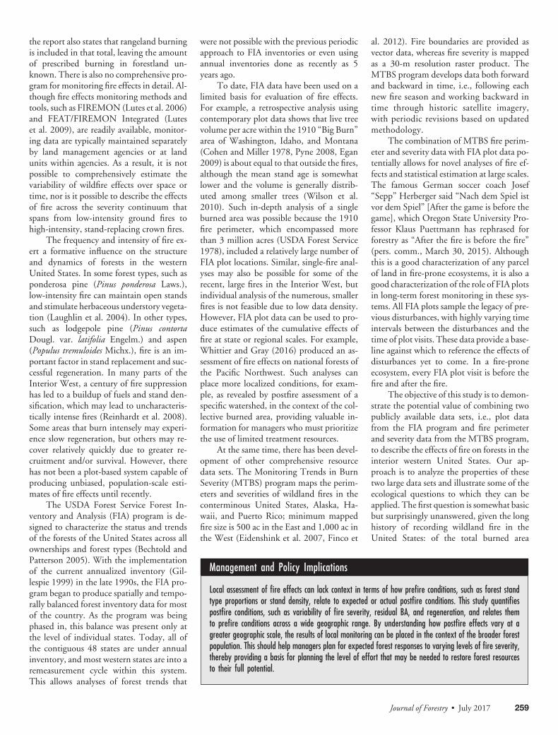
fire severity classification in relationship toprefire BA, many significant differences werefound among severity classes for tests of pre-fire versus postfire BA change (Figure 5; Ta-ble 3). This is an expected result, of course,because MTBS severity classifications arebased on changes in spectral signatures.However, this analysis also provides a poten-tial explanation of some of the mismatches

Figure 3. Ranked BA percent changes for conditions with prefire and postfire measure-ments. Percentile breakpoints are set at the percentiles of MTBS severity classes for the sameconditions. Inset numbers are counts of FIA plots by the MTBS severity classes within eachpercentile range. A perfect rank correlation would have all 165 MTBS “unburned/low”conditions in the lowest group, all MTBS “high” conditions in the highest group, and so on.The graph has been truncated at 100% increase (doubling of BA) for clarity.

Table 1. Summary of FIA and MTBS data used for this study.

StatePlot measurements within

burned perimeters1 % nonforest % forestTotal amountburned (ac)

No. of prefireforest plots

No. of postfireforest plots

Arizona 788 45.9 54.1 4,837,906 237 361Colorado 211 39.5 60.5 1,460,609 45 136Idaho 1,726 56.8 43.2 10,562,802 209 569Montana 967 35.1 64.9 6,050,826 170 589Nevada 1,390 89.9 10.1 8,138,978 27 131New Mexico 617 56.7 43.3 4,510,332 51 234Utah 503 57.6 42.4 3,332,783 119 227Wyoming 170 44.9 55.1 3,610,600 1 113Total 6,372 58.6 41.4 42,504,834 859 2,360

The percent forest and percent nonforest are based on the proportions of sampled forest and nonforest conditions on FIA plots within MTBS fire perimeters and thus represent the distribution of forestand nonforest within fire perimeters. The total acreage burned represents the combined area, or geographic union, of all MTBS fire perimeters in each state over the period of the study; areas that burnedmultiple times were not counted twice. The number of prefire forest plots includes all FIA plots that fall within MTBS perimeters but were measured before a fire occurrence and contained at least oneforest condition. Postfire plots are those within MTBS fire perimeters that were measured after a fire occurred and contained at least one forest condition.1 Plots included in this summary are those from the most recent evaluation group for each state (EVALID; see O’Connell et al. 2015).

Journal of Forestry • July 2017 263

shown in Figure 3. For all forest-type groupscombined, there was a significant and rela-tively regular progression of BA decreasewith increasing severity class. However,when major forest-type groups were consid-ered individually, severity classes 3 and 4 werenot significantly different in terms of live BAreduction even though most groups did showqualitative differences. The ability to statisti-cally distinguish between classes 1 and 2 andalso between classes 2 and 3 varied among themajor forest-type groups (Table 3).

A wide range of live BA was found onpostfire plots (n � 2,360); 35% of plots hadzero live BA and only 22% had more than 60ft2/ac (Figure 6). Because the calculated BAincludes only trees �5.0 in. in diameter

and most major tree species in this regiongrow too slowly to reach the 5-in. size classwithin 20 years (Burns and Honkala 1990a,1990b), postfire BA is probably composedalmost entirely of trees that survived firerather than new growth and thus representsresidual BA. We defined stand-replacing fireas plots with no live trees �5.0 in. in diam-eter. Although this high threshold appearsconservative (i.e., resulting in a minimal areaof stand-replacing fire), we should note thatthe FIA footprint samples are only 1⁄6 ac. Atlarger sampling footprints, the same sam-pling locations would undoubtedly capturelive residuals under some conditions. Be-cause of the small scale of the plot design, wedo not know whether a plot with 100%

mortality at the plot scale represents a high-severity patch within a variable severity fireor a typical part of a large, high-severitypatch. This distinction could be madethrough additional spatial analysis of MTBSseverity products and FIA plot locations.

At a regional scale, postfire plots thatburned fewer than 5 years before measure-ment have about 41% of the live BA ob-served at unburned plots (Figure 6). Postfiredead BA is about three times the dead BA atunburned plots, and it then gradually de-creases with time since fire. However, even atplots that burned 25 years or more before mea-surement, dead BA is nearly half that observedat recently burned plots (�5 years postfire).For a more detailed example of snag analysisusing FIA data, see Ganey and Witt (2017).Although some latent mortality may generateadditional dead BA, the large amount of deadBA present in all time intervals suggests thatmost of it was present just after the fire. In theInterior West, postdisturbance standing deadvolume does not reach its minimum until re-generating stands reach ages between 30 and60 years, according to a chronosequence anal-ysis by Garbarino et al. (2015). The downwardtrend in standing dead BA is consistent withthat trajectory, depending on when new stand-ing dead trees are produced by postfire regen-eration.

Postfire RegenerationBoth seedling and sapling demographic

classes show the expected immediate de-crease after fire (0–5 years), followed by ex-pected increases (Figure 7). Seedling densitypeaks 5–10 years after fire and then declinesafter 25 years postfire, as seedlings self-thin

Figure 4. Mean prefire total and live BA at FIA plots (n � 735) that burned betweenmeasurements by MTBS fire severity class. Prefire measurements occurred between 1993and 2002. Only the high-severity class (4) was significantly different from the other classes(prefire live BA, df � 3, F � 11.03, P < 0.0001; prefire total BA, df � 3, F � 11.63, P <0.0001). Error bars are �1 SEM live and total BA.

Table 2. Distribution of forest-type groups among the eight-state area, among remeasured FIA plots (n � 735) within MTBS perimeterswhere fires burned between plot measurements (measurement periods were 1993–2002 and 2003–2012), and among MTBS fireseverity classes.

Prefire forest-type group1

Proportion of totalforest land area in8-state study area2

Percentage of remeasuredplots in MTBSfire perimeters

No. of remeasuredplots in burned

areas

Percentage of remeasuredplots,by forest-type group, in each

fire severity class

1 2 3 4

Aspen/birch 5 2 12 0 25 50 25Douglas-fir 13 20 148 24 24 28 24Fir/spruce/mountain hemlock 16 15 113 14 20 22 43Lodgepole pine 8 8 57 32 23 14 32Other western softwoods 2 3 20 20 35 25 20Pinyon/juniper 37 20 145 26 37 25 12Ponderosa pine 9 23 172 23 38 25 14Western larch 1 1 5 20 20 40 20Woodland hardwoods 10 9 63 24 37 30 10All groups 100 100 735 23 31 25 22

1 Not shown: forest-type groups that occur in Interior West states but did not occur at T1 at remeasured plots.2 Total forest land area by forest-type group was obtained from FIA’s online EVALIDator estimation tool (apps.fs.fed.us/Evalidator/evalidator.jsp).

264 Journal of Forestry • July 2017

or move into the sapling size class. In con-trast, sapling density increases over a muchlonger period, and even at plots that burnedmore than 25 years before measurement sap-ling density continues to increase with timesince fire. Thus, this data set captures thepeak of regeneration in terms of seedlingdensity but does not capture the peak of sap-ling density. Instead, it illustrates that thepeak of postfire recruitment into the saplingsize class may occur more than 25 years afterfire and also reinforces the assumption thatmost postfire live BA consists of residual BA,or survivor trees for at least 25 years after fire.

Postfire Forest Type ChangesIn previous results we have shown fire-

induced reductions in BA and general pat-terns of recruitment. Although these metricsprovide some insight into stand-level

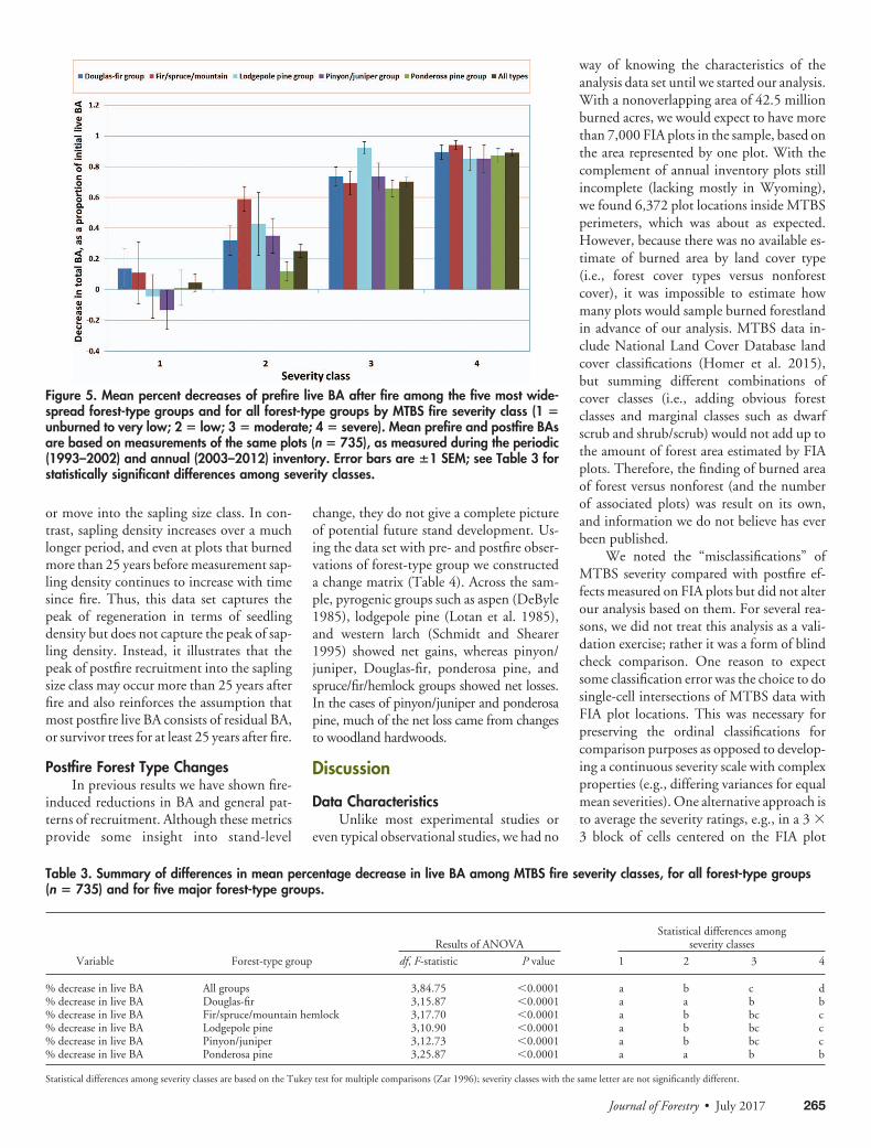
change, they do not give a complete pictureof potential future stand development. Us-ing the data set with pre- and postfire obser-vations of forest-type group we constructeda change matrix (Table 4). Across the sam-ple, pyrogenic groups such as aspen (DeByle1985), lodgepole pine (Lotan et al. 1985),and western larch (Schmidt and Shearer1995) showed net gains, whereas pinyon/juniper, Douglas-fir, ponderosa pine, andspruce/fir/hemlock groups showed net losses.In the cases of pinyon/juniper and ponderosapine, much of the net loss came from changesto woodland hardwoods.

Discussion

Data CharacteristicsUnlike most experimental studies or

even typical observational studies, we had no

way of knowing the characteristics of theanalysis data set until we started our analysis.With a nonoverlapping area of 42.5 millionburned acres, we would expect to have morethan 7,000 FIA plots in the sample, based onthe area represented by one plot. With thecomplement of annual inventory plots stillincomplete (lacking mostly in Wyoming),we found 6,372 plot locations inside MTBSperimeters, which was about as expected.However, because there was no available es-timate of burned area by land cover type(i.e., forest cover types versus nonforestcover), it was impossible to estimate howmany plots would sample burned forestlandin advance of our analysis. MTBS data in-clude National Land Cover Database landcover classifications (Homer et al. 2015),but summing different combinations ofcover classes (i.e., adding obvious forestclasses and marginal classes such as dwarfscrub and shrub/scrub) would not add up tothe amount of forest area estimated by FIAplots. Therefore, the finding of burned areaof forest versus nonforest (and the numberof associated plots) was result on its own,and information we do not believe has everbeen published.

We noted the “misclassifications” ofMTBS severity compared with postfire ef-fects measured on FIA plots but did not alterour analysis based on them. For several rea-sons, we did not treat this analysis as a vali-dation exercise; rather it was a form of blindcheck comparison. One reason to expectsome classification error was the choice to dosingle-cell intersections of MTBS data withFIA plot locations. This was necessary forpreserving the ordinal classifications forcomparison purposes as opposed to develop-ing a continuous severity scale with complexproperties (e.g., differing variances for equalmean severities). One alternative approach isto average the severity ratings, e.g., in a 3 �3 block of cells centered on the FIA plot

Figure 5. Mean percent decreases of prefire live BA after fire among the five most wide-spread forest-type groups and for all forest-type groups by MTBS fire severity class (1 �unburned to very low; 2 � low; 3 � moderate; 4 � severe). Mean prefire and postfire BAsare based on measurements of the same plots (n � 735), as measured during the periodic(1993–2002) and annual (2003–2012) inventory. Error bars are �1 SEM; see Table 3 forstatistically significant differences among severity classes.

Table 3. Summary of differences in mean percentage decrease in live BA among MTBS fire severity classes, for all forest-type groups(n � 735) and for five major forest-type groups.

Variable Forest-type group

Results of ANOVAStatistical differences among

severity classes

df, F-statistic P value 1 2 3 4

% decrease in live BA All groups 3,84.75 �0.0001 a b c d% decrease in live BA Douglas-fir 3,15.87 �0.0001 a a b b% decrease in live BA Fir/spruce/mountain hemlock 3,17.70 �0.0001 a b bc c% decrease in live BA Lodgepole pine 3,10.90 �0.0001 a b bc c% decrease in live BA Pinyon/juniper 3,12.73 �0.0001 a b bc c% decrease in live BA Ponderosa pine 3,25.87 �0.0001 a a b b

Statistical differences among severity classes are based on the Tukey test for multiple comparisons (Zar 1996); severity classes with the same letter are not significantly different.

Journal of Forestry • July 2017 265

location. This would have required analysisof all 30 annual severity data sets, which wasbeyond the scope of this project. Anotheralternative, suggested by C.A. Kolden (pers.comm., Sept. 25, 2015), is to drop MTBSseverity classes in favor of using the burnratio data used to derive severity classes. Thisapproach has the advantage of relating twosets of continuous variables (i.e., burn ratiosand computed FIA variables). Both ap-proaches merit future investigations and arecurrently in development.

At full implementation, annual FIAdata provide a spatially and temporally bal-

anced sample of forestland. However, al-though annual inventory was started in2000 in the Interior West, annual inventoryimplementation was phased in from 2000 to2011. In fact, 2014 was the first year that theannual sample was spatially balanced acrossall eight Interior West states. At this time,seven of the eight states have entered a cycleof annual inventory remeasurement. As a re-sult, although the patchy history of FIA in-ventory in the Interior West has imposedlimitations on the current analysis, futureanalyses have potential to be much morestraightforward and informative.

Effects of Prefire Conditions on Severityand Postfire Residuals, Regeneration,and Forest Type Change

Our analysis examines the effect ofstand density and forest type on fire, and theeffects of fire severity on stand residual struc-ture, composition, and regeneration. Thepurpose of these analyses was not specifichypothesis testing. Rather it was an explora-tion of the potential usefulness of the com-bination of two large, geographically com-prehensive data sets.

Our analysis of the effect of prefire BAon fire severity showed that fire in higher-density stands tended to result in higher se-verity classifications, whereas there was poorseparation between adjacent classes and nodifference at all between the two lowestclasses. Although this might be an indicationof a threshold effect, we must also considerthe part of our analysis that showed rela-tively poor separation of severity classifica-tion in the BA change ranking analysis (Fig-ure 4). Perhaps improvements in severityclassification procedures can result in bet-ter alignment of MTBS severity classesand plot-based observations of change,thereby providing greater separation ofchange among severity classes.

In contrast to the generalized approachof looking at all burned plots in aggregate,stratification of data by prefire forest-typegroups revealed differences across the rangeof MTBS severity classes (Figure 5). Inter-estingly, within the highest two severityclasses the amount of BA change as a propor-tion of prefire BA was very similar amongthe major forest-type groups. The exceptionto this pattern was for lodgepole pine, whichexperienced similar rates of mortality in themoderate and severe MTBS classes. Thisraises the question of whether the data reflecta tendency for lodgepole pine stands to besimilarly affected across a range of fire sever-ity or whether MTBS procedures do not ad-equately separate areas of moderate and highseverity in lodgepole pine stands. On thesurface that question would seem to be cir-cular because severity classification is basedon spectral signature change, but there maybe other factors that make lodgepole pinethe exception among the types we analyzed.Given that the other four types show rela-tively clear separation between the propor-tional BA change in moderate and severeclasses, the lack of a difference in lodgepolepine merits a closer look. Within the twolowest severity classes, the differences amongforest types appear greater, but there are few

Figure 6. Chronosequence of mean live and dead BAs for prefire (n � 859 plots) andpostfire (n � 2,360 plots) plots, with data from postfire plots shown by 5-year postfireintervals. Error bars are �1 SEM.

Figure 7. Chronosequence of mean sapling and seedling density for prefire (n � 859 plots)and postfire (n � 2,360 plots) plots, with data from postfire plots shown by 5-year postfireintervals. Error bars are �1 SEM.

266 Journal of Forestry • July 2017

cases for which the differences are signifi-cant. However, for each forest type, thedifferences in the proportional changesbetween the unburned/low and low classestended to be significant. This result suggeststhat some of the misclassifications found inthe ranked change analysis may be related tocertain forest types.

Our analysis of postfire BA shows thattotal mortality occurs on a minority ofburned forest acres. This is somewhat ex-pected, because even in the large and severefires of recent years, there is a mixture of fireeffects. What is not well known, however, ishow the proportions of severity class havebeen changing over time. The currentlyavailable approach is to rely on MTBS clas-sifications (e.g., Dillon et al. 2011), but thismethodology carries forward any MTBSclassification errors. There are open ques-tions regarding the limitations inherent inMTBS classifications (Kolden et al. 2015).FIA data can serve as a consistent source ofground-truth information and will charac-terize fire effects in greater detail than is pos-sible using spectral signatures.

For example, our analysis characterizesthe distribution of postfire residual BA ofboth the live and standing dead stand com-ponents. Based on seedling and stand originrecords associated with these conditions,about half of the area classified as severeappears to be regenerating naturally. This islikely to be a conservative estimate becauseerrors of commission in seedling counts arerare, but it is common to have regenerationrecorded in crew notes when none is talliedon the microplots. The regeneration statusof such plots will only be determined as re-measurement progresses and seedlings crossthe size threshold (5 in. dbh/drc) to be cap-tured on the subplots. In the majority of

burned forest area, a live tree component,frequently accounting for substantial BA, re-mains after fire and appears to persist. Thissuggests that the residual component has theopportunity to contribute to understory re-initiation (Oliver 1981) in a large fraction ofburned forest. Our generalized view of standdynamics after fire shows that this is occur-ring, with the expected postfire increase ofseedling-sized trees occurring up to 10–20years after fire, and subsequent graduationinto the sapling size class, which peaks atleast 25 years after fire. The next cycle ofmeasurements will provide valuable infor-mation on the trajectories of stands burnedduring the past 30 years, which may includeregeneration failures in addition to the doc-umented successes. These detailed observa-tions are important in the context of severityclassification, because one of the major con-cerns about large areas of severely burnedforestland is the extent to which they willadequately regenerate. The systematic sam-ple provided by FIA provides a frameworkfor monitoring regeneration success.

Beyond the simple issue of recordingregeneration, a major goal of the FIA pro-gram is to capture changes in the makeup offuture forests. From an ecological perspec-tive, the story is complex: high-severity firesin forest types such as lodgepole pine andaspen tend to favor these types (DeByle1985, Lotan et al. 1985), whereas in pinyon/juniper and spruce-fir, high-severity firegenerally favors earlier successional states.We found evidence of this using the limitedset of remeasured plots from which a forest-type group change matrix was derived (Ta-ble 4). Across the sample, pyrogenic speciessuch as aspen (DeByle 1985), lodgepole pine(Lotan et al. 1985), and western larch(Schmidt and Shearer 1995) showed net

gains, whereas pinyon/juniper, Douglas-fir,ponderosa pine, and spruce/fir/hemlockgroups showed net losses. In the cases of pin-yon/juniper and ponderosa pine, much ofthe net loss came from changes to woodlandhardwoods. This might be expected becausethese types tend to include a component ofspecies that sprout after fire, such as Gambeloak (Quercus gambelii Nutt.) (Harper et al.1985). In these cases, the sprouting speciescould account for the majority of the livecomponent for many years after severe fire andwould be recognized by field crews as the dom-inant species. Over all types, more than one-third of stands sampled before fire changedtype after fire. What has yet to be assessed iswhether these changes are expected as parts ofsuccessional cycles, or if some are state changesthat are possibly related to fire severity andother factors, such as climate. Again, the in-creasing body of data provided by continuousmonitoring will allow many of these questionsto be answered.

Although this analysis has produced in-teresting and perhaps encouraging resultswith respect to future forests, we cautionthat this is a preliminary analysis, given thelimited set of remeasurement plots available.Fortunately, as of the 2015 field season,seven of the eight Interior West states will bein a remeasurement cycle, so remeasurementdata will accumulate rapidly. In the InteriorWest states, remeasurement will occur at therate of approximately 3,000 forested condi-tions per year, with about one-third of thoseoccurring in areas that have burned withinthe past 25 years. Equally important are thetwo-thirds of plots in the yet-unburned por-tion of Interior West forests, because theywill serve as an unburned baseline for futurefires. As burned area accumulates in the fu-ture, this baseline will allow further analysis

Table 4. Prefire/postfire forest-type group change matrix (n � 735 plots).

Prefire forest-type group (n)

Postfire forest-type group

Aspen/birch Douglas-firFir/spruce/mountain

hemlockLodgepole

pineOther western

softwoodsPinyon/juniper

Ponderosapine

Westernlarch

Woodlandhardwoods

Aspen/birch (12) 7 1 1 1 2Douglas-fir (148) 8 101 7 7 1 12 4 8Fir/spruce/mountain hemlock (113) 13 10 54 30 2 1 1 1Lodgepole pine (57) 2 1 3 49 1 1Other western softwoods (20) 1 1 5 3 5 1 1 3Pinyon/juniper (145) 2 7 2 1 92 4 36Ponderosa pine (172) 2 8 20 108 33Western larch (5) 1 4Woodland hardwoods (63) 1 8 3 51Total (gain/loss) 35 (�23) 128 (�20) 73 (�40) 92 (�35) 9 (�11) 123 (�22) 131 (�41) 9 (�5) 132 (�69)

Some minor forest-type groups have been omitted, so prefire and postfire totals do not match.

Journal of Forestry • July 2017 267

of postfire conditions in the context of pre-fire conditions, providing direction for fu-ture management.

These analyses were done at a large re-gional scale, so there is much opportunityfor dissection of the results at smaller scales.In addition, we expect that the use of ancil-lary variables (e.g., stand density, composi-tion, vertical structure, understory and deadwoody fuel loadings, and climate data) couldfurther inform some of our analyses, such asthe effects of predisposing conditions on fireseverity. Although many of these character-istics have been examined in other studies,FIA’s continuous monitoring allows analysisand inference to population scales. Despitethe fact that much remains unknown, ourwidespread systematic sample allows somegeneralizations about fire effects in the Inte-rior West states. Different forest types havedifferent proportions of area in each fire se-verity class. These proportions can be refer-enced to existing studies on historic fire se-verity and can be used as baseline values forcomparison in the future.

Literature CitedARNER, S.L., S. WOUDENBERG, S. WATERS, J. VIS-

SAGE, C. MACLEAN, M. THOMPSON, AND M.HANSEN. 2001. National algorithms for deter-mining stocking class, stand size class, and foresttype for Forest Inventory and Analysis plots. In-ternal Rep. USDA Forest Service, Northeast-ern Research Station. Available online at www.fia.fs.fed.us/library/sampling/docs/supplement4_121704.pdf; last accessed Sept. 3, 2015.

BECHTOLD, W.A., AND P.L. PATTERSON (EDS.).2005. The enhanced Forest Inventory and Anal-ysis program—National sampling design and es-timation procedures. USDA Forest Service,Gen. Tech. Rep. SRS-80, Southern ResearchStation, Asheville, NC. 85 p. https://www.treesearch.fs.fed.us/pubs/20371.

BURNS, R.M., AND B.H. HONKALA (TECH. CO-ORDS.). 1990a. Silvics of North America, Vol. 1:Conifers. USDA Forest Service, Agri. Handbk.654, Washington, DC. 675 p.

BURNS, R.M., AND B.H. HONKALA (TECH. CO-ORDS.). 1990b. Silvics of North America, Vol.2: Hardwoods. USDA Forest Service, Agri.Handbk. 654, Washington, DC. 877 p.

COHEN, S., AND D. MILLER. 1978. The big burn:The Northwest’s fire of 1910. Pictorial HistoriesPublishing Co., Missoula, MT. 96 p.

DEBYLE, N.V. 1985. The role of fire in aspenecology. In Proc.—Symposium and workshopon wilderness fire, 1983 November 15–18. Mis-soula, Montana, Lotan, J.E., B.M. Kilgore,W.C. Fisher, and R.W. Mutch (tech. coords).USDA Forest Service, Gen. Tech. Rep. INT-182, Intermountain Forest and Range Experi-mental Station, Ogden, UT. 326 p.

DILLON, G.K., Z.A. HOLDEN, P. MORGAN, M.A.CRIMMINS, E.K. HEYERDAHL, AND C.H. LUCE.

2011. Both topography and climate affected for-est and woodland burn severity in two regions ofthe western US, 1984 to 2006. Ecosphere 2(12):art130. doi:10.1890/ES11-00271.1.

EGAN, T. 2009. The big burn: Teddy Roosevelt andthe fire that saved America. Houghton MifflinHarcourt, Boston, MA. 324 p.

EIDENSHINK, J., B. SCHWIND, K. BREWER, Z.ZHU, B. QUAYLE, AND S. HOWARD. 2007. Aproject for monitoring trends in burn severity.Fire Ecol. 3(1):3–21. doi:10.4996/fireecology.0301003.

ENVIRONMENTAL SYSTEMS RESEARCH INSTITUTE.2011. ArcGIS desktop, release 10.2.2. Environ-mental Systems Research Institute, Redlands, CA.

FINCO, M., B. QUAYLE, Y. ZHANG, J. LECKER,K.A. MEGOWN, AND C.K. BREWER. 2012.Monitoring trends and burn severity (MTBS):Monitoring wildfire activity for the past quar-ter century using Landsat data. P. 222–228 inMoving from status to trends: Forest Inventoryand Analysis (FIA) symposium 2012, 2012 De-cember 4–6, Baltimore, Maryland, Morin,R.S., and G.C. Liknes (comps.). USDA ForestService, Gen. Tech. Rep. NRS-P-105, North-ern Research Station, Newtown Square, PA[CD-ROM]. https://www.treesearch.fs.fed.us/pubs/42750.

GANEY, J.L., AND C. WITT. 2017. Changes insnag populations on National Forest Systemlands in Arizona, 1990s to 2000s. J. For.115(2):103–111. doi:10.5849/jof.2016-062.

GARBARINO, M., R. MARZANO, J.D. SHAW, AND

J.N. LONG. 2015. Environmental drivers ofdeadwood dynamics in woodlands and forests.Ecosphere 6(3):art30. doi:10.1890/ES14-00342.1.

GILLESPIE, A.J. 1999. Rationale for a national annualforest inventory program. J. For. 97(12):16–20.http://www.ingentaconnect.com/contentone/saf/jof/1999/00000097/00000012/art00007.

GOEKING, S.A. 2015. Disentangling forestchange from forest inventory change: A casestudy from the US Interior West. J. For.113(5):475–483. doi:10.5849/jof.14-088.

HARPER, K.T., F.J. WAGSTAFF, AND L.M. KUN-ZLER. 1985. Biology management of the Gambeloak vegetative type: A literature review. USDAForest Service, Gen. Tech. Rep. INT-179, In-termountain Forest and Range ExperimentStation, Ogden, UT. 31 p.

HOMER, C.G., J.A. DEWITZ, L. YANG, S. JIN, P.DANIELSON, G. XIAN, J. COULSTON, N.D.HEROLD, J.D. WICKHAM, AND K. MEGOWN.2015. Completion of the 2011 National LandCover Database for the conterminous UnitedStates-Representing a decade of land coverchange information. Photogramm. Eng. RemoteSens. 81(5):345–354. doi:10.1016/S0099-1112(15)30100-2.

KOLDEN, C.A., A.M.S. SMITH, AND J.T. ABATZO-GLOU. 2015. Limitations and utilisation ofMonitoring Trends in Burn Severity productsfor assessing wildfire severity in the USA. Int. J.Wildl. Fire 24(7):1023–1028. doi:10.1071/WF15082.

LAUGHLIN, D.C., J.D. BAKKER, M.T. STODDARD,M.L. DANIELS, J.D. SPRINGER, C.N. GILDAR,A.M. GREEN, AND W.W. COVINGTON. 2004.Toward reference conditions: Wildlife effects

on flora in an old-growth ponderosa pine for-est. For. Ecol. Manage. 199(1):137–152. doi:10.1016/j.foreco.2004.05.034.

LOTAN, J.E., J.K. BROWN, AND L.F. NEUEN-SCHWANDER. 1985. Role of fire in lodgepole pineforests. P. 133–152 in Lodgepole pine: The speciesand its management—Symposium proceeding,Baumgartner, D.M., R.G. Krebill, J.T. Arnott,and G.F. Weetman. (comps. and eds.). Wash-ington State University, Pullman, WA. 381 p.

LUTES, D.C., N.C. BENSON, M. KEIFER, J.F. CAR-ATTI, AND S.A. STREETMAN. 2009. FFI: A soft-ware tool for ecological monitoring. Int. J. Wildl.Fire 18(3):310–314. doi:10.1071/WF08083.

LUTES, D.C., R.E. KEANE, J.F. CARATTI, C.H.KEY, N.C. BENSON, S. SUTHERLAND, AND L.J.GANGI. 2006. FIREMON: Fire effects monitor-ing and inventory system. USDA Forest Service,Gen. Tech. Rep. RMRS-GTR-164-CD, RockyMountain Research Station, Fort Collins, CO[CD-ROM]. https://www.treesearch.fs.fed.us/pubs/24042.

MELVIN, M.A. 2015. 2015 National prescribedfire use survey report. Tech. Rep. 02-15, Coali-tion of Prescribed Fire Councils, Inc. 17 p.Available online at https://docs.google.com/a/prescribedfire.net/viewer?a�v&pid�sites&srcid�cHJlc2NyaWJlZGZpcmUubmV0fGNvYWxpdGlvbi1vZi1wcmVzY3JpYmVkLWZpcmUtY291bmNpbHN8Z3g6NWY5NTQ5ZDg3ODVmYTBhMw.

MONITORING TRENDS IN BURN SEVERITY. 2014.Monitoring Trends in Burn Severity (MTBS)Data access: National MTBS1taset (data re-lease: April 2014). MTBS Project, USDA For-est Service/US Geological Survey. Availableonline at www.mtbs.gov/data/individualfiredata.html; last accessed Sept. 3, 2015.

O’CONNELL, B.M., E.B. LAPOINT, J.A. TURNER,T. RIDLEY, S.A. PUGH, A.M. WILSON, K.L.WADDELL, AND B.L. CONKLING. 2015. TheForest Inventory and Analysis database: Data-base description and user guide version 6.0.2 forphase 2. Available online at www.fia.fs.fed.us/library/database-documentation/current/ver60/FIADB%20User%20Guide%20P2_6-0-2_final-opt.pdf; last accessed Aug. 30, 2015.

OLIVER, C.D. 1981. Forest development inNorth America following major disturbances.For. Ecol. Manage. 3:153–168. doi:10.1016/0378-1127(80)90013-4.

PYNE, S.J. 2008. Year of the fires: The story of thegreat fires of 1910, rev. ed. Mountain PressPublishing Company, Missoula, MT. 320 p.

REINHARDT, E.D., R.E. KEANE, D.E. CALKIN,AND J.D. COHEN. 2008. Objectives and consid-erations for wildland fuel treatment in forestedecosystems of the interior western United States.For. Ecol. Manage. 256(12):1997–2006. doi:10.1016/j.foreco.2008.09.016.

SAS INSTITUTE, INC. 2009. Base SAS 9.2 proce-dures guide. SAS Institute, Inc., Cary, NC.1705 p.

SCHMIDT, W.C., AND; R.C. SHEARER. 1995. Larixoccidentalis: A pioneer of the North AmericanWest. P. 33–37 in Ecology and management ofLarix forests: A look ahead: Proc. of an interna-tional symposium, 1992 October 5–9; Whitefish,Montana. USDA Forest Service, Gen. Tech.

268 Journal of Forestry • July 2017

Rep. GTR-INT-319, Intermountain ResearchStation, Ogden, UT.

US DEPARTMENT OF AGRICULTURE FOREST SER-VICE. 1978. When the mountains roared: Storiesof the 1910 fire. Rep. R1–78-30, Idaho Pan-handle National Forests, Coeur d’Alene, ID.Report R1–78-30. Available online at www.foresthistory.org/ASPNET/Publications/region/1/1910_fires/index.htm; last accessedMay 5, 2015.

US DEPARTMENT OF AGRICULTURE FOREST SER-VICE. 2013. Interior West Forest Inventory andAnalysis field procedures. Available online atwww.fs.fed.us/rm/ogden/data-collection/pdf/iwfia_p2_60.pdf; last accessed Feb. 17, 2015.

US DEPARTMENT OF AGRICULTURE FOREST SER-VICE. 2014. Fiscal year 2015 budget justifica-tion. Available online at www.fs.fed.us/sites/default/files/media/2014/25/2015-BudgetJustification-030614.pdf; last accessed Apr.17, 2015.

WESTERN FORESTRY LEADERSHIP COALITION.2010. The true cost of wildfire in the westernUS. Western Forestry Leadership Coalition,Lakewood, CO. April 2010 update. Availableonline at wflccenter.org/priority-issues/wildland-fire/; last accessed Mar. 11, 2015.

WHITTIER, T.R., AND A.N. GRAY. 2016. Treemortality based fire severity classificationfor forest inventories: A Pacific Northwest

national forests example. For. Ecol. Manage.359:199–209. doi:10.1016/j.foreco.2015.10.015.

WILSON, M.J., L.T. DEBLANDER, AND K.A. HAL-VERSON. 2010. Resource impacts of the 1910fires: A Forest Inventory and Analysis (FIA)perspective. Presented at 1910 fires: A centurylater. Wallace, Idaho, May 20–22, 2010.USDA Forest Service, Rocky Mountain Re-search Station, Forestry Sciences Laboratory,Interior West Forest Inventory and AnalysisProgram, Ogden, UT.

ZAR, J.H. 1996. Biostatistical analysis, 3rd ed.Prentice Hall, Upper Saddle River, NJ. 662 p.plus appendices.

Journal of Forestry • July 2017 269